Journal of Marine Systems 148 (2015) 152–166

Contents lists available at ScienceDirect

Journal of Marine Systems

j ourna l homepage: www.e lsev ie r .com/ locate / jmarsys

Fresh oxygen for the Baltic Sea — An exceptional saline inflow after adecade of stagnation

V. Mohrholz ⁎, M. Naumann, G. Nausch, S. Krüger, U. GräweLeibniz-Institute for Baltic Sea Research Warnemünde, Germany

⁎ Corresponding author.E-mail addresses: Volker.Mohrholz@io-warnemuende

Michael.Naumann@io-warnemuende.de (M. Naumann),Guenther.Nausch@io-warnemuende.de (G. Nausch),Siegfried.Krueger@io-warnemuende.de (S. Krüger), Ulf.Gr(U. Gräwe).

http://dx.doi.org/10.1016/j.jmarsys.2015.03.0050924-7963/© 2015 The Authors. Published by Elsevier B.V

a b s t r a c t

a r t i c l e i n f o

Article history:Received 23 February 2015Received in revised form 10 March 2015Accepted 11 March 2015Available online 18 March 2015

Keywords:Baltic SeaMajor Baltic inflowWater exchangeInflow statistics

The ecological state of the Baltic Sea depends crucially on sufficiently frequent, strong deepwater renewal on theperiodic deep water renewal events by inflow of oxygen rich saline water from the North Sea. Due to the strongdensity stratification these inflows are the only source for deep water ventilation. Since the early eighties of thelast century the frequency of inflow events has dropped drastically from 5 to 7 major inflows per decade to onlyone inflow per decade.Wide spread anoxic conditions became the usual state in the central Baltic. The raremajorBaltic inflow (MBI) events in 1993 and 2003 could interrupt the anoxic bottomconditions only temporarily. Aftermore than 10 years without a major Baltic inflow events, in December 2014 a strongMBI brought large amountsof saline and well oxygenated water into the Baltic Sea. Based on observations and numerical modeling, the in-flow was classified as one of the rare very strong events. The inflow volume and the amount of salt transportedinto the Baltic were estimated to be with 198 km3 and 4 Gt, respectively. The strength of the MBI exceeded con-siderably the previous 2003 event. In the list of the MBIs since 1880, the 2014 inflow is the third strongest eventtogetherwith theMBI in 1913. This infloweventwill most probably turn the entire Baltic deepwater from anoxicto oxic conditions, with substantial spread consequences for marine life and biogeochemical cycles.

© 2015 The Authors. Published by Elsevier B.V. This is an open access article under the CC BY-NC-ND license(http://creativecommons.org/licenses/by-nc-nd/4.0/).

1. Introduction

TheBaltic Sea is a semi-enclosed sea in thehumid zoneof thenorthernhemisphere. Two narrow and shallow straits, the Belt Sea and the Sound(Fig. 1), connect the Baltic Sea to the North Sea, and thus to the worldocean. The restrictedwater exchange through the straits is of high impor-tance for environmental conditions in the entire Baltic Sea (Elken andMatthäus, 2008;Matthäus et al., 2008). Due to the high freshwater runofffrom the catchment area, outflow conditions are generally dominating.The salt balance of the Baltic is maintained by sporadic inflows of highlysaline waters from the North Sea. Saline inflows can be of barotropic orbaroclinic type. Barotropic inflows are forced by sea level differences be-tween theKattegat and theArkonaBasin, caused bywind and air pressureforcing (Franck et al., 1987;Wyrtki, 1954;Matthäus, 2006). These inflowsmay occur at any time of the year, although its probability is higher in thewinter season, when the wind forcing is at its seasonal maximum.

.de (V. Mohrholz),

aewe@io-warnemuende.de

. This is an open access article under

Baroclinic inflows usually occur during long calm periods in summer,and aredrivenby the salinity gradient between the Baltic and theKattegat(Knudsen, 1900; Hela, 1944; Feistel et al., 2003a, 2003b, 2006; Mohrholzet al., 2006). The saline inflows maintain the brackish character of theBaltic waters, with mean surface salinity of about 7 and bottom salinitiesbetween 11 and 13 in the central basins. The residence time of salinewater in the Baltic is about 30 years (Franck et al., 1987). The strong ver-tical stratification of the Baltic Sea blocks the direct ventilation of thedeeper layers by deep convection during the winter and during storms.Only the layers above the permanent halocline at 60 to 70 m depth arein contact with the atmosphere and are directly supplied with oxygen.The deep water is renewed exclusively by lateral advection, namely bythe eastward spreading of dense waters from saline inflow events. Thus,the oxygen content of the saline inflow waters is of crucial importancefor the environmental conditions in the deep water. Oxygen content ofinflowing water depends on the season when the inflows occur. In sum-mer the oxygen concentration of inflowing water is reduced due to hightemperatures and by oxygen demand of biogeochemical processes. Infact, summer inflows do not considerably contribute to the ventilationof deep water. Mainly inflows between October and March may supplyoxygen to the deep Baltic basins. Further, an inflow needs a certain vol-ume of saline water to reach the bottom layer of the central basins.Small inflows are soon diluted on their pathway toward the central Baltic.

the CC BY-NC-ND license (http://creativecommons.org/licenses/by-nc-nd/4.0/).

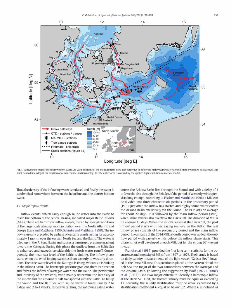
Fig. 1. Bathymetric map of the southwestern Baltic Sea with positions of the measurement sites. The pathways of inflowing highly saline water are indicated by dashed bold arrows. Theblack dashed lines depict the location of across channel sections of Fig. 14. The entire area is covered by the applied high resolution numerical model.

153V. Mohrholz et al. / Journal of Marine Systems 148 (2015) 152–166

Thus, the density of the inflowingwater is reduced andfinally thewater issandwiched somewhere between the halocline and the denser bottomwater.

1.1. Major inflow events

Inflow events, which carry enough saline water into the Baltic toreach the bottom of the central basins, are called major Baltic inflows(MBI). These are barotropic inflow events, forced by special conditionsof the large scale atmospheric circulation over the North Atlantic andEurope (Lass andMatthäus, 1996; Schinke andMatthäus, 1998). The in-flow is usually preceded by a phase of easterly winds lasting for approx-imately 1 month over the eastern North Sea and the Baltic. The water ispiled up in the Arkona Basin and causes a barotropic pressure gradienttoward the Kattegat. During this phase the outflow from the Baltic Seais enhanced and exceeds considerably the fresh water runoff. Conse-quently, the mean sea level of the Baltic is sinking. The inflow phasestarts when the wind forcing switches from easterly to westerly direc-tions. Then the water level in the Kattegat is rising, whereas it is sinkingin the Arkona Basin. The barotropic pressure gradient alters its directionand forces the inflow of Kattegat water into the Baltic. The persistenceand intensity of the westerly wind mainly determine the intensity ofthe inflow and the amount of salt transported into the Baltic. To fill upthe Sound and the Belt Sea with saline water it takes usually 2 to3 days and 2 to 4 weeks, respectively. Thus, the inflowing saline water

enters the Arkona Basin first through the Sound and with a delay of 1to 3weeks also through the Belt Sea, if the period ofwesterlywinds per-sists long enough. According to Fischer and Matthäus (1996) a MBI canbe divided into three characteristic periods. In the precursory period(PCP), just after the inflow has started and highly saline water entersthe Arkona Basin exclusively via the Sound. The PCP lasts on averagefor about 22 days. It is followed by the main inflow period (MIP),when saline waters also overflow the Darss Sill. The duration of MIP ison average 10 days. When the inflow ceases at the Darss Sill, the postinflow period starts with decreasing sea level in the Baltic. The realinflow phase consists of the precursory period and the main inflowperiod. In our study of the 2014MBI, a fourth periodwas added: the out-flow period with easterly winds before the inflow phase starts. Thisphase is not well developed at each MBI, but for the strong 2014 eventit was.

Franck et al. (1987) provided the first long term statistics for the oc-currence and intensity of MBIs from 1897 to 1976. Their study is basedon daily salinity measurements of the light vessel “Gedser Rev”, locat-ed in the Darss Sill area. This position is placed at the eastern rim of theBelt Sea, the major of the two connections between the Kattegat andthe Arkona Basin. Following the suggestion by Wolf (1972), Francket al. (1987) used two major criteria to identify a barotropic inflowat the Darss Sill. First, the bottom salinity must be equal or exceeding17. Secondly, the salinity stratification must be weak, expressed by astratification coefficient G equal or below 0.2. Where G is defined as

154 V. Mohrholz et al. / Journal of Marine Systems 148 (2015) 152–166

G = 1 − (surface salinity/bottom salinity). Both ensure a barotropicinflow process with highly saline water throughout the water column.These conditions must be persistent for at least five consecutive daysto classify the inflow as a MBI. Using this scheme, Franck et al.(1987) derived an empirical intensity index QFMS87, which was definedby following Eq. (1):

Q FMS87 ¼ 2k d−1 þ 7:143 S −131:429: ð1Þ

Where k is the time span in days where the two above-mentionedcriteria are fulfilled at the position of the light vessel “Gedser Rev”,and S is the mean practical salinity over the same period. The indexQFMS87 has a range between zero and 100, which describes the largestpossible MBI. Based on the QFMS87 index it was shown that the MBIsoccur exclusively between August and April, with a maximum inDecember. Maximum intensity and duration of inflows were observedbetween November and January. During their investigation periodfrom 1897 to 1976 five to seven MBIs per decade were detected,which appear in groups interrupted by periods of 1 to 4 years withoutMBI.

The main weakness of the intensity index QFMS87 was the lack of anyobservational information about the inflow process through the Sound.The volume transports between the Kattegat and the Arkona Basin areusually split between the Belt Sea and the Sound with a ratio between70 to 30% (Jacobsen, 1980; Jakobsen and Trébuchet, 2000) and 80 to20% (Mattsson, 1996). The real ratio may vary within this range, dueto different forcing conditions of the particular inflow events. Thus, ad-ditional information from the Sound transport is needed to obtain agood estimate of the total Inflow volume and salt transport of an inflow.

Fischer andMatthäus (1996) reviewed the QFMS87with special focuson the Sound transports. They derived a new quantitative intensitymeasure QFM96 (Eq. (2)). It is based on the total amount of salt M ingiga tons, which is transported through the Belt Sea (MB) and theSound (MS) into the Baltic Sea during an inflow event.

Q FM96 ¼ MS þMB

0:1 Gt: ð2Þ

To identify the inflow at the Sound two rules were introduced ac-cording to the criteria for the Darss Sill area. First: the surface salinityat the Sound must be equal or higher than 17, and the current mustbe directed into the Baltic Sea. Second: all days of the PCP (but notmore than 15) and all days of the MIP, which meet first condition,must be taken into account for the transport estimations. To make theintensity index unitless, themass of salt is divided by 1011 kg (=0.1 Gt).

The statistics of MBI was extended until 2006 by Matthäus (1993),Schinke andMatthäus (1998) andMatthäus et al. (2008). The frequencyand intensity of MBIs changed drastically between 1976 and 1983. Longlasting stagnation periods without any MBI became the usual state inthe deep basins. Only in 1993 (Dahlin et al., 1993; Jakobsen, 1995;Matthäus and Lass, 1995; Liljebladh and Stigebrandt, 1996) and in2003 (Feistel et al., 2003b, 2006; Lehmann et al., 2004) MBIs were ob-served that were able to ventilate the deep Baltic basins for 1 to2 years. Since 2003 only a weak MBI occurred in late autumn 2010which transported about 1 Gt salt into the Baltic. However, this inflowwas too weak to have significant impact on the conditions in the deepBaltic basins.

Beside the observational estimates of the volume and salt transportof the MBIs, several attempts were made to reconstruct the inflows innumericalmodels. For instance,Meier et al. (2003) estimated the inflowvolume of high-saline water (S N 17) of the 1993 inflow as 137 km3,which is close to the observations of 135 km3 (Matthäus, 1993;Matthäus and Lass, 1995). Moreover, Meier et al. (2003) could alsoreproduce the nearly equal volume partitioning of the inflowing waterbetween Darss Sill and the Sound.

Especially the 2003 inflow event has been used as a benchmark test.Lehmann et al. (2004) computed the total volume transport as 240 km3.In contrast, Hofmeister et al. (2011) or Fu (2013) gave a lower transportvalue with 167 km3 and 179 km3 respectively. The spread of the modelresults around the estimation of 200 km3, based on observations (Feistelet al., 2003b), shows that still an optimal modeling strategy is missing.Crucial are the horizontal resolution in the Danish Straits, due to theircomplex bathymetry, but also the choice of the vertical coordinate sys-tem (z-level, Lehmann et al., 2004, or terrain-following coordinates,Burchard et al., 2005, or Hofmeister et al., 2011).

The nutrient conditions in the Baltic Sea react strongly on the alter-nation between inflow and stagnation periods. This has been studiedamong others by Fonselius (1967, 1970), Nehring (1989), Nehring andMatthäus (1991) and Nausch et al. (2003). In the presence of oxygen,phosphate is fixed in the sediments and onto sedimenting particles asan iron-III-hydroxyphosphate complex (cf. Balzer, 1984). If the systemturns from oxic to anoxic conditions, accompanied by the change ofthe redox potential, this complex is reduced by hydrogen sulfide (Hilleet al., 2005). Phosphate and iron(II)ions are liberated leading to anincrease in the phosphate and iron concentrations in the deep water.Moreover, inorganic nitrogen compounds are affected by the interplaybetween oxygen and hydrogen sulfide. Under oxic conditions, they arepresent almost exclusively as nitrate whereas nitrite is only an interme-diate step of the nitrification. Under anoxic conditions, however, nitrateis denitrified tomolecular nitrogengas (N2). Ammoniumwhich is trans-ferred from the sediments or liberated duringmineralization processes,cannot be oxidized under these conditions and is enriched. Due to ver-tical mixing processes (Reissmann et al., 2009), enriched nutrients canbe transported upwards and when reaching the euphotic surfacelayer, may determining to a large extent the intensity of primaryproduction. However, looking from an ecosystem perspective, thesevertical transports across pycnoclines are not sufficiently understoodin time and quantity.

In this study we investigate the development and the dynamics ofthe exceptional MBI, observed in December 2014. This MBI has thepotential to stop the stagnation period, which lasts since the 2003 MBIin the deep Baltic basins.

2. Material and methods

For the description of inflow dynamics and the transport calcula-tions a data set from various sources was used. It consists of hydro-graphic and meteorological data from the permanent MARNETstations Darss Sill and Arkona Basin, sea level data from gauges atLandsort Norra, Hornbaek, Gedser, Viken and Klagshamn, surface tem-perature (SST) and surface salinity (SSS) observations from the ferry“Finnmaid”, CTD and thermosalinometer data from the cruise EMB092of R/V “Elisabeth Mann-Borgese” (15th–19th December 2014). The po-sitions of the particular stations and measuring sites are depicted inFig. 1. Additionally, meteorological data and topographic data frompublic sources were used. The data cover the time period from the 1stNovember to 31st December 2014.

2.1. The MARNET stations Darss Sill and Arkona Buoy

The first indications for theMBI 2014 were detected at theMARNETstation Darss Sill. For this study, time series of wind, current and salinityat the Darss Sill and in the central Arkona Basinwere obtained from twopermanent autonomous stations of the German Marine MonitoringNetwork (MARNET). Both stations, Darss Sill and Arkona Basin(Fig. 1), are developed and operated by the Leibniz Institute for BalticSea ResearchWarnemünde (IOW) (Krüger, 1997, 2000). The main pur-pose of the stations is the permanent observation of meteorological andhydrographic parameters for the environmental monitoring of theBaltic Sea, with special focus on the water exchange between theNorth and Baltic Seas (BSH, 2014).

155V. Mohrholz et al. / Journal of Marine Systems 148 (2015) 152–166

The MARNET station Darss Sill (54°42′N, 12°42′E) is located at thetransition between the Belt Sea and the Arkona Basin, 25 km east ofthe real topographic Darss Sill. The station consists of a bottommounted, buoyancy stabilized pole as mounting platform for thesensors. Wind speed and wind direction are measured 10 m above thesea surface. Temperature and salinity measurements are performed atsix depth levels in 2, 5, 7, 12, 17, and 19 m depths with SeaBird SBE 37thermosalinometers. Additionally, in 7 and 19mdepths oxygen optodesaremounted. Current speed anddirection ismeasured between 2mand20 m depth by a bottom mounted, upward looking ADCP (RDI WH600 kHz) with 1 m vertical resolution.

TheMARNET station Arkona Basin (54°53′N, 13°52′E) is positioned atthe southern rimof the central Arkona Basin in themain pathway of east-ward spreading saline inflows. The station is constructed as a semi divingspar buoy, fixed with two heavy anchors at the sea floor. The equipmentconsists of various meteorological and oceanographic sensors, similar tothe station Darss Sill. For our studywe used only the temperature and sa-linity observations, which are performed in eight depth levels at 2, 5, 7,16, 25, 33, 40, and 43m depths with SeaBird SBE 37 thermosalinometers.

Real-time data of both stations are transmitted hourly to BSH andIOW via METEOSAT and GSM. The real-time data of these stationsenabled the exact temporal and first quantitative identification of theactual salt water inflow.

2.2. Sea level data

The tide-gauge data of the Swedish stations Landsort Norra, Vikenand Klagshamn are provided by the online-data-server of the SwedishMeteorological andHydrological Institute (SMHI, 2015). Thedata are re-lated to the Swedish reference level RH2000, and were converted intomean sea level (MSL) by annual varying local factors because of thepostglacial isostatic uplift of Scandinavia. These factors are for LandsortNorra−10.4 cm, Viken−7.5 cmand Klagshamn−12.58 cm, calculatedafter SMHI (2014) for the year 2014. The sea level at Landsort Norra, inthe south of Stockholm, represents themean filling level of the Baltic Sea(Feistel et al., 2008; Jacobsen, 1980; Lisitzin, 1974). The sea level gaugesViken and Klagshamn located in the north and south of the Sound areused to estimate the inflowing volume by tide-gauge differences.

For the Danish tide-gauge stations at Hornbaek and Gedser the datawere extracted from thewebsite of the Baltic Operational Oceanograph-ic System (BOOS, 2014). The data is listed in hourlymeans and providedin MSL as reference level. These stations show the inflow activity ofthe Great Belt. All sea level data time series have temporal resolutionof 1 h.

2.3. “Finnmaid” ferry data

The Finnish cargo ferry “Finnmaid” commutes regularly at 2 day in-tervals between Lübeck and Helsinki. On its 1100 km long track itcrosses nearly the entire Baltic from the southwestern corner to theGulf of Finland in the northeastern part. In frame of the Alg@line projectin 2007 the ferry was equipped by the Finnish Marine Research Centre(SYKE) with a ferrybox system. It measures a continuous time seriesdata of temperature, salinity, chlorophyll-a fluorescence and turbidityin surface water. In cooperationwith the IOW the systemwas extendedwith a sensor for carbon dioxide partial pressure (pCO2). The scientificequipment is regularly maintained when the ferry stays in Lübeckport. The temperature and salinity data of November and December2014were used to observe the temporal development of the surface sa-linity front from the Kadet Furrow toward the Arkona Basin. The spatialresolution of the temperature and salinity data is about 200 m.

2.4. Hydrographic data from cruise EMB092

From 15th to 19th December 2014, the German research vessel“Elisabeth Mann-Borgese” performed one of its regular cruises in the

western Baltic. The main focus of the cruise was the maintenance ofthe MARNET stations Arkona Basin and Oder Bank, and on testing ofnew scientific equipment. Beside these tasks 15 CTD profiles weremea-sured at 11 stations in the area of the central Arkona Basin to the DarssSill from17th to 19thDecember (see Fig. 1), to obtain information aboutthe initial inflow phase in the southwestern Baltic. The CTD system con-sists of a SeaBird 911+ probe, mounted on a sampling rosette. It wasequipped with 13 free flow tubes of 5 L volume which allow directwater sampling during the downward moving process. The CTD probehad double sensors for each parameter and was calibrated in the IOWlaboratory. The data quality was cross checked by additional tempera-ture measurements, and laboratory analyses of salinity and oxygensamples taken with the water sampler. After validation the remaininguncertainties of the main parameters temperature, salinity and oxygenamount to 0.005 K, 0.006 and 4 μmol l−1, respectively. The CTD winchhad a newly developed swell compensation system controlled bymotion sensor signals of the vessel to prevent vertical loops duringprofiling.

The CTD data were used to obtain characteristic properties of thetwo saline water bodies that entered the Arkona Basin via the GreatBelt/Darss Sill and the Sound. The depth of the salinity 17 isohalinewas identified as upper boundary of the Great Belt/Darss Sill water.The boundary of this water mass to the Sound water was determinedby salinity of 21, and higher turbidity values. The estimated limitswere used to model these surfaces for the area covered by the CTDprofiles. Rectangular grids of 500 m grid point distance were gener-ated by geostatistical methods (kriging with semi-variogram analy-sis) using the software tool SURFER. In addition with a grid of theseafloor, obtained from the iowtopo2_rev3 dataset (Feistel et al.,2008; Seifert et al., 2001), volumes of the different inflowwater bod-ies were calculated for covered area. With an extrapolation of thesedata, the total inflow volume was estimated for the entire ArkonaBasin.

The RV “Elisabeth Mann Borgese” is equipped with a thermo-salinograph, which continuously collected temperature and salinitydata of the surface water. These data were used to complement thesurface data recorded by the “Finnmaid” ferry.

2.5. Baltic topography

The bathymetric dataset “iowtopo2_rev3” compiled by Seifertet al. (2001) is the most dense, quality checked and freely availabledataset for the entire region of the Baltic Sea. This data set wasused to generate regular grids of different resolutions (250 m,500 m grid point distances) for the western Baltic by the samegeostatistical methods as described above. Also the topographic in-formation in Fig. 1, the data about the cross sections at Darss Silland Sound, and the volume calculations for the basins are based onthis bathymetric dataset.

2.6. Transport estimates

For the calculations of transports through the straits betweenKattegatandArkona Basin, namely the Sound and the Belt Sea, differentmethodswere applied.

The total transport between Kattegat and the Baltic for time scaleslonger than 3 days can be derived from the change of water volume inthe Baltic. The volume change of the Baltic was estimated using thesea level change at Landsort Norra in the western Gotland Basin.This sea gauge is located closely to the node lines of the main seichemodes of the Baltic and represents its filling state (Feistel et al., 2008;Jacobsen, 1980; Lisitzin, 1974). Thus, the effect of seiches is very littleon this sea gauge. To exclude the residual impacts of short term fluctu-ations a fourth order low pass Butterworth filter with 3-day cut offperiod was applied to the original data. Seiches with a typical periodof 25 h or less (Jönsson et al., 2008; Wübber and Krauss, 1979),

156 V. Mohrholz et al. / Journal of Marine Systems 148 (2015) 152–166

as well as the impact of short term meteorological patterns areremoved. The volume change of the Baltic was estimated using Eq. (3).

ΔV ¼ 3:8 km3cm−1 � Δη−1:3 km3d−1 � Δt: ð3Þ

WhereΔV is the volume transport through theDanish straits in km3,Δη is the sea level change at Landsort Norra in cm, and Δt is the timespan of sea level change in days. This equation includes the meanclimatological freshwater surplus from runoff and precipitation of1.3 km3d−1. The sea level is measured in whole centimeters. Thus, theuncertainty of sea level change for a certain period is 1 cm in the begin-ning plus 1 cm in the end. The uncertainty of 2 cm in sea level changeresults in an uncertainty of 8 km3 in volume change. The total transportestimatedwith the sea level change at Landsort Norra splits into the twopathways via the Sound and the Darss Sill.

Fischer and Matthäus (1996) derived an empirical relation for thesplit of transport between Sound and Belt Sea from an analysis ofabout 90 MBI events between 1880 and 1976. They found that duringthe PCP and the first 5 days of theMIP the distribution of volume trans-port between the Darss Sill (VDS) and the Drogden Sill (VDR) is close toEq. (4).

VDR ¼ 0:326 VDS r ¼ 0:991ð Þ: ð4Þ

The inflow at the Drogden Sill stopped usually at day five of theMIP.Afterwards an outflow is observed at the Drogden Sill, whereas the in-flow at the Darss Sill continued. The outflow at the Drogden Sill fromday five of the MIP onwards was estimated with:

VDR ¼ −0:115 VDS r ¼ 0:958ð Þ: ð5Þ

We applied Eqs. (4) and (5) to the total transport, derived from thesea level change at Landsort Norra to obtain an estimate for the DarssSill and the Drogden Sill transport.

A secondmethod to estimate transports in the connecting straits be-tween Kattegat and the Arkona Basin is based on local sea level differ-ences Δη. In the first approximation the flow through the straits isdriven by the along channel barotropic pressure gradient, which is bal-anced by the friction in the channel. Usually a quadratic frictional law(Eq. (6)) is applied, with a flow resistance coefficient K (e.g. Jacobsen,1980; Omstedt, 1987).

Δη−A ¼ K f Q Qj j: ð6Þ

Q is the transport through the channel, and A is an empirical correc-tion factor the baroclinic pressure gradient. Some studies include thiscorrection into the empirical flow resistance coefficient.

a)

Fig. 2. a) Monthly mean of sea level air pressure at station Warnemünde in 2014 (solid red lin(2015). b) 3 days mean values of sea level at station Landsort Norra in 2014 (solid red line) co

A further linear term can be introduced into Eq. (6) to account forthe geostrophic adjustment of the channel flow (Mattsson, 1996).

Δη−A ¼ K1Q þ K f Q Qj j with K1 ¼ fgH

and K f ¼cDL

gH3W2 : ð7Þ

The factors K1 and Kf can be derived from the theory of channel flow.Usually, Kf is adjusted to the observed transport by fitting the drag coef-ficient cD.H, L andW are themean depth, length andwidth of the chan-nel. Here f and g are the inertial frequency and the earth acceleration.

Both equations were applied. However, the difference of about 3%for the Sound is rather small. The uncertainty of the method is givenby Mattsson (1996) with approximately 10%. Thus, we used finally thesimple quadratic equation with Kf = 2.03 ∗ 10−10 s2m−5, and A =0.018 m for the Sound which is also in the range of Kf from1.6 ∗ 10−10 s2m−5 to 2.6 ∗ 10−10 s2m−5 given by Jakobsen et al. (1997).

The application of the same equation to theBelt Sea transports is alsopossible and often done, but it results in higher uncertainties than forthe Sound. Due to the greater water depth of the Belt Sea the impactof the baroclinic pressure gradient between theKattegat and theArkonaBasin is considerably higher. It has been shown by earlier studies thatthe resistance coefficient Kf depends on the stratification in the BeltSea. Mean values for the resistance coefficient were given by Pedersen(1978) with Kf = 4.0 · 10−11 s2/m5, and Jacobsen (1980) with Kf =3.8 · 10−11 s2/m5. Recent investigations from Jakobsen et al. (2010) sug-gest a minimum resistance coefficient for the entire Belt Sea between2.0 and 3.0 · 10−11 s2/m5. For the transport estimates in this study a re-sistance coefficient of 2.5 · 10−11 s2/m5was used, since during aMBI theflow through the Belt Sea is mainly barotropic and the resistance coeffi-cient should be close to the minimum.

The transport estimations described above are indirect methods.The volume and salt transports at the Darss Sill were also estimatedfrom direct current and salinity measurements of the MARNETstation Darss Sill. Badewien (2002) has shown that the transportscalculated for the vertical profile at this measuring site provide agood estimate for the entire section Darss Sill. For this purpose thecurrent and salinity data were extrapolated horizontally andweight-ed with the width of the cross section at each depth level. However,we found that the extrapolation method according to Badewien(2002) results in a significant overestimation of transports. Thus,the calculated transports were calibrated with the total volumechange of the Baltic, derived from sea level change at LandsortNorra, and corrected for the Sound transports. For this calibrationwe used the period with rapid rising sea level from 3rd Decemberto the 18th December 2015. The correction factor was determinedwith cDS = 0.79. For the Sound no current measurements are avail-able for the measuring period. Thus, the two indirect methods wereused to estimate the transports there.

b)

e) compared to the climatological mean 1947–2005 (dashed black line), data from DWDmpared to the mean of the 10 year period 2005–2014 (dashed black line).

Fig. 3. Wind forcing in the western Baltic during November/December 2014. Data were obtained from the MARNET station Darss Sill.

157V. Mohrholz et al. / Journal of Marine Systems 148 (2015) 152–166

2.7. Numerical model

Finally, we estimated the volume and salt flux through the cross-sections at Darss Sill and the Drogden Sill with the help of a numericalmodel. The model provided hourly mean values of velocity and salinityat every grid point. Thus, the model provided also a direct estimate ofthe fluxes. We employed the General Estuarine Transport Model(GETM) in a multi nested downscaling framework. GETM is a 3D free-surface primitive equation model using the Boussinesq and boundarylayer approximations. Vertical mixing is parameterized by means of atwo-equation k- turbulence model coupled to an algebraic second-moment closure. Advection of momentum, turbulent kinetic energy,and dissipation rate was done by a third‐order scheme and for tracerby a second‐order scheme (Klingbeil et al., 2014). The model has beensuccessfully applied to simulate inflow events into the Baltic Sea(Burchard et al., 2005), and was further used for climate downscalingand a statistical analysis of inflows in the western Baltic Sea (Gräweet al., 2013).

For the present setup, we discretized the model domain with a hor-izontal resolution of 1/3 nautical mile (app. 600 m). The model domaincovers the Danish Straits and the western Baltic. The open boundariesare located along 57°N in the Kattegat and along the 17°17.5′Emeridianat the eastern rim of the Bornholm Basin. In the vertical we used 50terrain-following adaptive layers, with a zooming toward stratificationand a minimum layer thickness of 0.3 m. Except the increase in verticalresolution, the present setup is identical to the one used by Klingbeil

Fig. 4.Observed hourly sea level at Landsort Norra (thin blue line) and lowpassfiltered time seriat Landsort Norra from the numerical model.

et al. (2014). A detailed description and validation of the used setup isgiven in Klingbeil et al. (2014).

At the open boundaries of the model domain, the water elevations,depth averaged currents, as well as salinity and temperature profilesare prescribed. This external forcing was taken from a model of theNorth Sea–Baltic Sea (NSBS) with a horizontal resolution of 1 nauticalmile and 50 vertical layers. To account for large scale variations andstorm surges, NSBS was nested into a depth-averaged storm surgemodel of the North Atlantic with a resolution of 5 nautical miles.

The atmospheric forcing was derived from the operational model ofthe GermanWeather Service with a spatial resolution of 7 km and tem-poral resolution of 3 h. The initial conditions for the model were takenfrom a running simulation, starting at the 1st January 2014.

3. Results

TheMBI 2014was forced by the typicalmeteorological sequence de-scribed in previous studies (Lass and Matthäus, 1996; Schinke andMatthäus, 1998). During autumn, September toNovember 2014, centralEurope and the Baltic Sea area weremainly influenced by high pressuresystems located over northeastern Scandinavia to eastern Europe andlow pressure systems over the northeast Atlantic. The sea level air pres-sure anomaly atWarnemündewas positive fromSeptember toDecember2014 (Fig. 2a).

Consequently, the wind situation was abnormally calm for thisseason with mostly SE, S to SW directions. The mean wind speed from

es, using a cutoff period of 3 days (bold red line). The dashed green line depicts the sea level

Belt SeaSound

Fig. 5. Sea level difference between Kattegat–Arkona Basin. Through the Belt Sea (Hornbaek–Gedser, solid blue line) and through the Sound (Viken–Klagshamn, dashed red line).

158 V. Mohrholz et al. / Journal of Marine Systems 148 (2015) 152–166

September to November 2014 was only 3.9 ms−1 at the stationWarnemünde. At the station Arkona, which is located on a high cliff42 m above mean sea level, the average wind speed from Septemberto November 2014 was 6.1 ms−1. There daily means of wind speedwere not exceeding 12 ms−1. Hourly means higher than 10.7 ms−1

(N5 Bft) were seldom with around 6.5% of the time and show amaximum of 16 ms−1 in these months. The wind speed was weak tomoderate, lower than 7.9 ms−1 (4 Bft) in 72.5% of the time. Arkona, inthe north of Rügen island, is the windiest station along the GermanNorth and Baltic Sea coast (Lefebvre and Rosenhagen, 2008) andshows more or less the situation at the open water in the southwesternpart of the Baltic Sea. In comparison, the coastal station Rostock–Warnemünde recorded wind speeds higher than 10.7 ms−1 in only1.9% of this timespan and 94.6% of the data had values below7.9ms−1. This longperiod of calmwind forcing andhigh air pressure re-sulted in a loweredmean sea level of the Baltic Sea. Since the beginningof September themean sea level showedvalues belowzero at the Swed-ish Landsort station in the central Baltic (Fig. 2b). Only a short phase ofsouthwest–westwinds from19th–29thOctober caused by lowpressuresystems up to 970 hPa over northern Europe and a long lasting highpressure area, spreading from western to eastern Europe, pushed thesea level at Landsort to positive values up to 12 cm above mean sealevel. This mainly calm weather situation of autumn 2014 is matchingthe inflow scenarios of Lass and Matthäus (1996) as well as SchinkeandMatthäus (1998). They described that a positive air pressure anom-aly in autumn and a resulting lowered mean sea level of the Baltic Seaoften coincide with the occurrence of MBIs in the following winterseason.

Between the 11th November and the first week of December 2014medium to strong easterly winds with average speed of 8.8 ms−1

were observed in the western Baltic (Fig. 3). The east winds forced anoutflow of Baltic surface water, followed by a drop in mean sea levelin the Baltic (Fig. 4). The long lasting phase with easterly winds wasinterrupted only for a fewdays between the 23rd and the26thNovember

Fig. 6. Salinity at the MARNET station Arkona in November/December 2014. A —

2014. On the 2nd December the easterly winds calmed down for about2 days. This stopped the outflow from the Baltic and the further drop insea level. An onset of persistent westerly winds occurred on the 5thDecember. During the following days the wind speed increased toabout 10 ms−1 and more. The resulting uplift of water in the easternNorth Sea and Kattegat and the corresponding local drop of sea level inthe Arkona Basin caused a steep barotropic pressure gradient betweenthe Kattegat and the Arkona Basin. This pushed a strong barotropic in-flow of saline North Sea water into the Baltic Sea. The heavy westerlywinds lasted until the 25th December. The average wind speed duringthe inflow phase was 11.4 ms−1. After the 25th December the windspeed decreased rapidly to about 5 ms−1 with changing directions.

According to the observed sea level at Landsort Norra (Fig. 4) the dif-ferent phases of the inflow were identified. The outflow period startedon the 7th November with a sea level of +10 cm. Afterwards the sealevel was decreasing continuously, only interrupted by a short increasearound the 26th November. The outflow period finished on 3rd Decem-ber, when the minimum sea level of −47 cm was reached. Afterwardsthe inflow phase started with the precursory period with rapidly risingsea level. The inflow phase, consisting of the precursory and the maininflow period, lasted until the 25th of December. Then the maximumsea level of +48 cmwas reached at Landsort Norra, and the post inflowperiod started with decreasing sea level. Fig. 4 also indicates that both,the filling state of the Baltic Sea and the dynamics of sea level patterns,are well reproduced by the numerical simulations.

The local sea level difference between the Kattegat and the westernArkona Basin is the driving force for the barotropic water exchangethrough the Belt Sea and the Sound. The sea level differences for theBelt Sea and the Sound were calculated from the tide gauges atHornbaek and Gedser, and Viken and Klagshamn respectively (Fig. 5).Generally, the behavior at both channels is very similar. During the out-flow period the sea level difference is negative, with mean values of−22.6 cm for the Belt Sea and −10.5 cm for the Sound. Only duringthe short interruptionof easterlywind forcing around the 25thNovember

9

9

9

AB

first saline overflow from the Sound, B — saline water from the Darss Sill.

21

17

9

21

131717

13

6

6

9

13

13

a)

b)

c)

Fig. 7.Observations of along channel velocity (a) and salinity (b) at the MARNET station Darss Sill in November/December 2014, compared with salinity from numerical model (c) at thesame position.

159V. Mohrholz et al. / Journal of Marine Systems 148 (2015) 152–166

where positive sea level differences were observed. During the inflowphase the sea level differences changed their sign and increased consid-erably. For the Belt Sea and the Sound the mean sea level differencesamount to +44.9 cm and +32.4 cm in the precursory period, and to+47.9 cmand+28.7 cm in themain inflowperiod.With the beginningof the post period the sea level differences dropped again to negativevalues.

Due to the shorter channel length, first highly saline water enteredtheArkonaBasin via the Sound around the 4thDecember. Unfortunately,there are no direct measurements from the Sound. However, atthe MARNET station Arkona the first inflow water was detected on12 December (Fig. 6), one day before the saline waters arrived at theDarss Sill (cf. also Fig. 7b). The salinity of this water mass increased in

7m depth19m depth

Fig. 8. Time series of oxygen concentration at the MARNET station Da

the following days to maximum values of about 22.6, observed 2 mabove the bottom on 15th December.

The advection time of inflowing water from the Drogden Sill to theMARNET station Arkona of approximately 8 days was very well inagreement to earlier observations (Lass and Mohrholz, 2003; Burchardet al., 2005; Sellschopp et al., 2006). On its pathway the entrainmentof ambient brackish water lowered the salinity of the inflowing water.Thus, the salinity at the Sound was assumed to be well above 23. Thiswas also supported by the direct CTDobservations that revealed bottomsalinities of 25 in the western Arkona Basin on 18th December.

The time series data from the Darss Sill station supplied a compre-hensive picture of the inflow process via the Belt Sea (Fig. 7). The out-flow period from 7th November to 3rd December is characterized by

rss Sill in 7 m (solid blue line) and 19 m depth (dashed red line).

Belt SeaSound

Fig. 9. Volume transport through the Belt Sea (solid blue line) and the sound (dashed red line) estimated from the sea level differences Hornbaek–Gedser and Viken–Klagshamn.

160 V. Mohrholz et al. / Journal of Marine Systems 148 (2015) 152–166

negative along channel velocities (outflow) throughout the water col-umn. Only two short baroclinic inflow pulses were observed between21st and 27th November. During the outflow period the salinity ofabout 8 indicated the outflow of brackish surface water. The baroclinicinflowpulses are also reflected in temporarily increased bottom salinity.The inflowphase at the Darss Sill started on 3rd Decemberwith positivealong channel velocities of 0.25 to 0.50ms−1. Since theBelt Seawaspre-viously flushed with low saline surface water, the salinity at the DarssSill remains initially at low values, and increased slowly only duringthe precursory period.With 9 days delay to the Sound, the highly salinewater was detected at the Darss Sill. On 13th December the salinityexceeded 17 in the entire water column. At this time no vertical salinitygradientwas observed at the Darss Sill station (Fig. 7b). The arrival timeof highly salinewater at the Darss Sill determines the end of the precur-sory period. With 10 days duration the PCP of the MBI 2014 was rathershort comparedwith themean duration of 22 days given by Fischer andMatthäus (1996).

The current direction at the Darss Sill remained positive during theentire main inflow period that lasted until the 25th December. Meancurrent velocity was about 0.2 to 0.3 ms−1. The bottom salinity in-creased during the entire MIP from 17 in the beginning to 22 on 25thDecember. At the Darss Sill the mean salinity was 18.56, averagedover theMIP. At the start of the post-period the surface salinity droppeddrastically to about 8, the usual value for Baltic surface water. The bot-tom salinity remained at high values for a fewdays. This indicates an on-going baroclinic leakage of highly saline bottomwater from the Belt Seainto the Arkona Basin, temporary interrupted by a reflux of highly salinewater from the Arkona Basin.

Fig. 7c demonstrates that themodel can reproduce the observationsvery well. Also small events like the baroclinic pulses between 21st and27th November 2014 are well represented. The modeled salinity atDarss Sill is in good agreement with the observed salinity profiles(Fig. 7c).

Fig. 8 depicts the oxygen concentrations measured at 7 and 19 mdepths at the Darss Sill. Due to the exchange with the atmosphere the

Fig. 10. Transports at the Darss Sill section calculated from themeasurements of current velocityports based on sea level difference Hornbaek Gedser (thin gray line and shaded area).

surface waters are well oxygenated during the months November andDecember. The oxygen saturation ranges between 95 and 100% in thesurface layer. In the bottom layer the oxygen concentration was nega-tively correlated with the salinity until the start of themain inflow peri-od. The higher saline waters of the baroclinic inflow pulses during theoutflow phase and in the PCP were oxygen depleted. These waterswere remainders of old saline bottom waters from the Belt Sea.The highly saline waters that enter the Baltic in the MIP were welloxygenated throughout the water column. Mean oxygen concentrationand temperature of the inflowing saline water at the Darss Sill were322 μmol l−1 and 6.29 °C, respectively.

For the estimation of total volume transports between the Baltic andthe North Sea Eq. (3) was applied to the low pass filtered sea levelmeasurements at the Landsort Norra. Since no actual runoff data wereavailable, we considered the climatological mean freshwater surplusof 1.3 km3d−1 for the calculation of volume transport. 242 km3 of brack-ish surface water left the Baltic during the outflow period until 3rdDecember, causing a drop in mean sea level of 55 cm. In the inflowphase a total inflow of 323 km3 was estimated. This was split into161 km3 for the PCP and 162 km3 for the MIP.

A second estimate for the volume transports was derived fromthe sea level differences between the Kattegat and the ArkonaBasin according to Eqs. (6) and (7) (Fig. 9). During the outflowperiod, the cumulated transports into the Belt Sea and the Soundamounted to −187 km3 and −45 km3, respectively. The sum of−232 km3 is 10 km3 less than the estimated from the sea levelchange at Landsort Norra. However, this is within the upper limitof the uncertainty of the method of 10%. During the inflow phasean inflow of 240 km3 and 64 km3 water was estimated for the BeltSea and the Sound. Also during the inflow phase the sum of304 km3 water was slightly lower than the 323 km3 estimated fromthe sea level change at Landsort Norra. The distribution of volumetransports between the Belt Sea and the Sound was 8:1.9 duringthe outflow period, and 8:2.1 during the inflow phase. This is closeto the relation of 8:2 given by Mattsson (1996).

and salinity at theMARNET station Darss Sill (bold blue line) compared to Darss Sill trans-

Fig. 11. Bottom salinity in the numerical model at MARNET station Darss Sill (solid blue line), Drogden Sill (dashed red line), and Gedser Rev (dotted green line).

161V. Mohrholz et al. / Journal of Marine Systems 148 (2015) 152–166

The volume and salt transports at the Darss Sill were also estimatedusing the time series data of current and salinity, observed at the perma-nent MARNET station Darss Sill (see Fig. 7). During the outflow phasefrom 7th November to 3rd December the net outflow through the BeltSea was calculated with −195 km3. The inflow volume amounted to110 km³ for the precursory period and 138 km3 for themain inflow pe-riod. In the first days of the post-period an additional baroclinic inflowof 9 km3 saline water was detected, which contributes to the totalamount of the MBI inflow volume. The volume transports at the DarssSill estimated from the sea level differenceHornbaek–Gedser and calcu-lated from the Darss Sill current data are compared in Fig. 10. Generally,both time series show a similar behavior, and the same magnitude oftransports. However, the transports derived from the direct currentmeasurements depict a higher temporal variability. The differencesare caused most probably by the local dynamics of the Darss Sill areaand baroclinic processes, which are not recognized in the transport es-timates based on sea level difference.

For the salt transport through the Sound only a rough estimate canbe given, because no direct salinity measurements were available. Thesalinity observations at the MARNET station Arkona and also the CTDprofiles from the western Arkona Basin indicated that the salinity ofthe inflowing water at the Sound was well above 23. This is confirmedby the modeled salinities. In contrast to the observational data, wherethe Practical Salinity is used as salinity scale, the model salinity isgiven as Absolute Salinity in units of g kg−1. Fig. 11 indicates thatthe inflowing water via the Sound had salinities between 21 and 25.

Table 1Summary of transport calculations. Netto volumes (V) in km3 transported during the particularsaline water into the Baltic. The last two rows (bold) summarize the volumes estimated from

Outflow period Precursory perio

Period 07.11.2014–03.12.2014 03.12. 2014–13.1

Vtotal [km3]Sea level change Landsort

−242 161

VSound [km3]Sea level difference Viken–Klagshamn

−45 30(26)0.60 Gt salt

VSound [km3]Numerical model

−67.5 37.50.59 Gt salt

VDarss Sill [km3]Sea level difference Hornbaek–Gedser

−187 103

VDarss Sill [km3]Current and salinity measurements atMARNET Darss Sill

−195 110

VDarss Sill [km3]Numerical model

−145.8 70.60.16 Gt salt

Vtotal [km3]VDarss Sill + VSound

Observations

−235 140(26)0.60 Gt salt

Vtotal [km3]VDarss Sill + VSound

Numerical model

−213.3 108.10.75 Gt salt

We used a salinity of 23 as mean value for the entire inflow period.Assuming, that the inflow water needs approximately 1 day to passthe Sound, 26 km3 highly saline water entered the Baltic in the PCP.This corresponds to a salt transport of 0.60 Gt. During the main inflowperiod another 34 km3 highly saline water added 0.78 Gt salt to thetotal salt transport of theMBI. The conversion between Practical Salinityand mass of salt (Absolute Salinity) was performed according to theinternational thermodynamic equation of seawater 2010 (IOC, SCORand IAPSO, 2010).

Since the estimated transport through the Sound was based on sev-eral assumptions, we used the numerical model to get an independentestimate of the through flow. Themodeled volume and salt flux throughthe Sound are close to the observations (compare Table 1). However,the GETM predicts slightly higher values. Nevertheless, the deviationsare less than 10%.

The salt transport at the Darss Sill amounted to 2.60 Gt for the MIPand 0.17 Gt for first days of the post inflow period. Again, the modelled values are 2.40 Gt close to the observational estimates. In addition,the transport values for the post-inflow are in good agreement.Table 1 summarizes the transport estimations from the differentmethods used for all phases of the MBI.

In order to compensate the lack of observational salinity and currentmeter data at the Drogden Sill an alternative approach was used to ver-ify the calculation of the volume transport via the Sound. The CTD data,gathered between of 17th and 19th December on a cruise of RV“ElisabethMann Borgese”, supplied a distribution of the different inflow

inflow periods. Numbers in brackets depict the fraction of inflowvolumes that carry highlyobservations and numerical model.

d Main inflow period Total inflow phase Post inflow

2.2014 13.12.2014–25.12.2014 03.12.2014–25.12.2014 25.12.2014–31.12.2014

162 323 −111

34(34)0.78 Gt salt

64(60)1.38 Gt salt

−22

38.90.85 Gt salt

76.41.44 Gt salt

−33.4

137 240 −59

138(138)2.60 Gt salt

248(138)2.60 Gt salt

−43(9)0.17 Gt salt

134.42.24 Gt salt

205.02.40 Gt salt

−63.50.11 Gt salt

172(172)3.38 Gt salt

312(198)3.98 Gt salt

−65(9)0.17 Gt salt

173.33.09 Gt salt

281.43.84 Gt salt

−970.11 Gt salt

Fig. 12. Vertical salinity distribution along a transect from the Darss Sill to the center of Arkona Basin (17th to 19th December 2014). Positions of CTD stations and transect are depictedin Fig. 1.

162 V. Mohrholz et al. / Journal of Marine Systems 148 (2015) 152–166

watermasses in thewestern Arkona Basin. Fig. 12 shows the vertical sa-linity distribution along a transect from the Darss Sill to the center ofArkona Basin. The inflowing saline water masses from the Belt Sea andthe Sound depict different properties. According to the time seriesdata from the MARNET stations Darss Sill and Arkona Basin the salinityof Belt Sea water ranged between 17 and 21, whereas the salinity of theSoundwater was higher than 21. Thus, the isohalines with salinity of 17and 21were used to identify the both inflowwater bodies. In theArkonaBasin the Sound water showed a maximum salinity of 26 and a meanvalue of 22.8. Its mean temperature and oxygen content were of 8.2 °Cand 275 μmol l−1. The water that entered the Arkona Basin via theBelt Sea had a lower mean salinity of 18.9, a temperature of 7.3 °C,and an oxygen concentration of 307 μmol l−1. Beside these parametersthe Sound water depicted a higher turbidity compared to the Belt Seawater (not shown). Due to its lower density the Belt Sea water issandwiched between the old Arkona Basin water and the highly salineSound water.

For the Arkona Basin section of the CTD transect, with water depthgreater than 30m, the fractions of the particular water masses were es-timated. In the period of 17th–19th December 62% of the volumeconsisted of less saline surface water and uplifted former bottomwater. 18.8% were covered by highly saline water from the Belt Seaand 19.2% by water that originated from the Sound. A linear extrapola-tion to the total volume of the Arkona Basin of 225 km³ supplied a veryraw, but independent estimate of the inflow volumes. The derived vol-umes of Belt Seawater and Soundwater are 42 km³ and 43 km³, respec-tively. The calculated transport of highly saline water via the Darss Sill

Fig. 13.Hovmöllerplot of surface salinity (left) and depth profile (right) along a transect from thMARNET stations Darss Sill and Arkona buoy (dotted lines). The dashed line indicates the histo

amounted to 54 km3 till 17th December. This increased until the 19thDecember to about 73 km3. The cumulated inflow volume of highlysaline Sound water was 40 km3 and 44 km3 on the 17th and 19thDecember, respectively. This compares with the range of uncertaintieswith the volume estimates derived from the CTD data.

Measurements of sea surface salinity (SSS) from the MARNET sta-tions Darss Sill and Arkona Basin were combined with data gatheredon board of the ferry “Finnmaid” and the RV “Elisabeth Mann-Borgese” to investigate the temporal behavior of the surface salinityfront in theDarss Sill area (Fig. 13). The SSS front depicted by the salinity17 isohaline reached the MARNET station Darss Sill on 13th Decemberwith the start of theMIP. TheMARNET station Darss Sill was the easternmost position of the salinity 17 isohaline. Further to the east the highlysaline water descents underneath the surface waters of the ArkonaBasin. On 21st December the SSS front moved westward to 12.5°Ebetween the MARNET station and the Kadet Furrow, and remained atthis position until the end of the MIP.

4. Discussion

Themain aims of the presented study are the investigation of the de-velopment and the dynamics of the exceptional ChristmasMBI 2014, itsclassification and the estimation of its possible impact on the Baltic Seaecosystem. For classification in principle two scales are available: the in-tensity index QFMS87 developed by Franck et al. (1987) and the new in-tensity scale QFM96 by Fischer andMatthäus (1996). The latter one is themore appropriate scale, since it is based on the total salt amount

e Kadet Furrow (Gedser Rev) to the central Arkona Basin. Data from “Finnmaid” ferry andrical position of light vessel Gedser Rev.

461 000 m2 612 500 m2

52 750 m2844 000 m2

a) b)

c) d)

Fig. 14.Geometry and cross section area of across channel sections atGedser Rev (a), DarssSill (b). MARNET station Darss Sill (c) and Drogden Sill (d). The dashed line in panel(c) depicts the position of the MARNET station Darss Sill.

163V. Mohrholz et al. / Journal of Marine Systems 148 (2015) 152–166

transported into theBaltic Sea.However, in order to compare our resultsto earlier studies we also calculated the intensity index QFMS87. Usingthis intensity scale the MBI 2014 has an intensity index of QFMS87 =26.1 (k = 12.46 d, S = 18.56), based on the observations at theMARNET station Darss Sill. For comparison, the previous MBI in 2003had an intensity index of 12.1 on the same scale (Feistel et al., 2003b).

It should be recognized that the application of the FMS87 index ontothe actual Darss Sill data might be inconsistent. The MARNET StationDarss Sill is located 46.9 km eastward of the position of the light vesselGedser Rev and 21 km eastward, or downstream of the topographicDarss Sill. Assuming an upper limit of mean current velocity of0.4 ms−1 the inflowing water needs approximately 32 h from GedserRev to MARNET station Darss Sill. This will lead to an underestimationof inflow intensity FMS87 for events that are deduced from data of theMARNET Darss Sill station. The temporal difference of the presence ofSSS greater 17 between the Kadet Furrow station and the MARNET sta-tion Darss Sill is illustrated in Fig. 13. To improve the estimation of in-flow intensity FMS87 one can apply a correction of k for the distancebetween Gedser Rev and MARNET station Darss Sill using an offsetk0 = 2*32 h = 2.6 days. Using this approach, the QFMS87 has the morerealistic value of 31.3 for the MBI 2014.

There is also a significant difference in topography between thecross sections at Gedser Rev, Darss Sill and MARNET station DarssSill (compare Fig. 14). The Gedser Rev section has the minimal crosssection area of 0.461 km2. The Darss Sill section depicts the shallowest

Fig. 15. Stratification coefficient G in the numerical model at MARNET station Darss Sill (solid bwhen stratification coefficient G was lower than 0.2 and bottom salinity was higher than 17 areDrogden Sill, bottom — Gedser Rev).

bottom depth of 18 m. The cross section area at the MARNET stationDarss Sill is approximately double as large (0.844 km2) as the crosssection area at the Gedser Rev, and the maximum bottom depth is23 m. Thus, the section at the MARNET station Darss Sill is often notcompletely covered by inflowing saline waters passing the Gedser Revsection.

The MARNET station Darss Sill is closely located to the western rimof the Arkona Basin. The inflowing saline water starts to subduct inthe vicinity of the station. Therefore the salinity front fluctuates aroundthis position during the inflowphase. Especially in the secondhalf of theMIP the surface layer at the MARNET station Darss Sill is covered occa-sionally by low saline surface water, whereas the inflow continues atdeeper layers (compare Fig. 7). In this phase the increasing salinity ofinflowing waters forces a faster subduction. Due to the shallow layerof low saline surface waters the stratification coefficient G exceeds theMBI limit of 0.2.

To identify an inflow as MBI, Franck et al. (1987), and also Fischerand Matthäus (1996) used the criteria, that for at least five consecutivedays the bottom salinitymust be equal to or exceeding 17, and the strat-ification coefficient Gmust be equal to or below 0.2. Minor MBIs whichfulfill these criteria at the Gedser Rev, may not do this at the MARNETstation Darss Sill. Due to the shift of the continuous observations fromthe Gedser Rev to the MARNET station Darss Sill in the 1980s, mostprobably some weak to moderate MBIs was not identified as a MBI,since they did not fulfill the MBI criteria at the MARNET station DarssSill. This view is supported by the complete lack of weak MBIs since1983, which should be the MBI class with the highest frequency.However, the necessary revision of the MBI statistics exceeds theframe of the present study and will be done in a future work.

The impact of the measuring position can be illustrated for the MBI2014 by using the modeled salinity. The application of the MBI criteriato the positions Gedser Rev and MARNET station Darss Sill resulted ina huge difference in the FMS87 index. At Gedser Rev the MBI criteriais fulfilled for 19.3 days. Regarding the mean salinity of 20.5, theFMS87 index of the MBI 2014 is 53.6 which is a very strong inflow atthis scale (N45). In contrast, the duration of 11.4 days and the mean sa-linity of 19.4 at theMARNET station Darss Sill revealed an inflow inten-sity of 30.1 on the FMS87 scale, pointing on a medium to strong inflow.Fig. 15 depicts the stratification coefficient G and the periods when theMBI criteria are fulfilled in the numerical model at the particular sta-tions. It shows an additional minor MBI in the first week of Decemberwhich is not seen at the MARNET station Darss Sill.

The use of salt transports for MBI classification, introduced byFischer and Matthäus (1996), will overcome the problem of measuringlocation. Between the 13th of December and the end of themain inflowphase on 25th December the cumulated transport into the Baltic via theDarss Sill amounts to 138 km3 saline water with 2.6 Gt salt (based onDarss Sill current and salinity measurements). It should be also men-tioned that during the post-inflow period a substantial amount of salt

lue line), Drogden Sill (dashed red line), and Gedser Rev (dotted green line). The periods,indicated by the bold colored lines at the bottom of the graph (top— Darss Sill, middle—

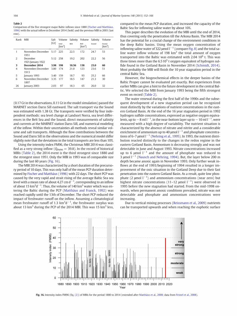
Table 2Comparison of the five strongest major Baltic inflows since 1880 (Fischer and Matthäus,1996) with the actual inflow in December 2014 (bold) and the previousMBI in 2003 (lastrow).

Rank MBI Salt[Gt]

Volumetotal

[km3]

SalinityBelt

VolumeBelt

[km3]

SalinitySound

VolumeSound

[km3]

1 November/December1951

5.17 225 22.5 172 24.7 53

2 December1921/January 1922

5.12 258 19.2 202 22.2 56

3 December 2014 3.98 198 18.56 138 23.0 604 November/December

19133.80 174 21.0 123 23.6 51

5 January 1993 3.40 159 18.7 93 25.2 666 November/December

18973.35 177 18.5 147 21.3 30

26 January 2003 2.03 97 18.3 65 26.0 32

164 V. Mohrholz et al. / Journal of Marine Systems 148 (2015) 152–166

(0.17Gt in the observations, 0.11 Gt in themodel simulation)passed theMARNET section Darss Sill eastward. The salt transport via the Soundwas estimated with 1.38 Gt. The transports were verified by four inde-pendent methods: sea level change at Landsort Norra, sea level differ-ences in the Belt Sea and the Sound, direct measurements of salinityand currents at the MARNET station Darss Sill, and numerical modelingof the inflow. Within their uncertainties all methods reveal similar vol-ume and salt transports. Although the flow contributions between theSound and Darss Sill in the observations and the numerical model differslightly note that the deviations in the total transports are less than 10%.

Using the intensity index FM96, the Christmas MBI 2014 was classi-fied as a very strong inflow (QFM96 = 39.8). In the record of historicalMBIs (Table 2), the 2014 event is the third strongest since 1880 andthe strongest since 1951. Only the MBI in 1993 was of comparable sizeduring the last 60 years (Fig. 16).

TheMBI 2014was characterized by a short duration of the precurso-ry period of 10 days. This was only half of themean PCP duration deter-mined by Fischer andMatthäus (1996)with 22 days. The short PCPwascaused by the very rapid and strait rising of the average Baltic Sea sealevel with amean rate of about 4.27 cmd−1, corresponding to an inflowof about 15 km3d−1. Thus, the volume of 140 km3 water which was en-tering the Baltic during the PCP (Matthäus and Franck, 1992) wasreached rapidly until the 13th of December. The short PCP reduced theimpact of freshwater runoff on the inflow. Assuming a climatologicalmean freshwater runoff of 1.3 km3d−1, the freshwater surplus wasabout 13 km3 during the PCP of the 2014 MBI. This was 15 km3 less,

no d

ata

- WW

II

no d

ata

- WW

I

Fig. 16. Intensity index FM96 (Eq. (2)) of MBIs for the period 1880 to 2014

compared to the mean PCP duration, and increased the capacity of theBaltic Sea for inflowing saline water by about 10%.

This paper describes the evolution of the MBI until the end of 2014,thus covering only the penetration till the Arkona Basin. The MBI 2014has the potential for a crucial change of the environment conditions inthe deep Baltic basins. Using the mean oxygen concentration ofinflowing salinewater of 322 μmol l−1 (compare Fig. 8) and the total sa-line water inflow volume of 198 km3 the total amount of oxygentransported into the Baltic was estimated with 2.04 106 t. This wasthree times more than the 6.5105 t oxygen equivalent of hydrogen sul-fide found in the Gotland Basin in November 2014 (Schmidt, 2014).Most probably the MBI will finish the 10 year stagnation period in thecentral Baltic Sea.

However, the biogeochemical effects in the deeper basins of theBaltic Proper cannot be evaluated yet exactly. But experiences fromearlierMBIs can give a hint to the future development in the central Bal-tic. We selected the MBI from January 1993 being the fifth strongestevent on record (Table 2).

The water renewal during the first half of the 1990s and the subse-quent development of a new stagnation period can be recognizedmost distinctly by the variations of nutrient concentrations in the east-ern Gotland Basin. At the end of the 16 year stagnation period in 1992hydrogen sulfide concentrations, expressed as negative oxygen equiva-lents, up to−8ml l−1, in the near-bottom layer up to−10ml l−1, weremeasured with a high degree of variability. The nutrient situation ischaracterized by the absence of nitrate and nitrite and a considerableenrichment of ammonium up to 40 μmol l−1 and phosphate concentra-tions of 6–7 μmol l−1 (Nehring et al., 1995). In 1993, the nutrient distri-bution reacted distinctly to the changes in the redox regime in theeastern Gotland Basin. Ammonium is decreasing strongly and was notdetectable in June and August 1993. Nitrate concentrations increasedup to 6 μmol l−1 and the amount of phosphate was reduced to3 μmol l−1 (Nausch and Nehring, 1994). But, the layer below 200 mdepth became anoxic again in November 1993. Only further weak in-flows at the end of 1993/beginning of 1994 resulted in a longer im-provement of the oxic situation in the Gotland Deep due to their fastpenetration into the eastern Gotland Basin. As a result, quite low phos-phate (2 μmol l−1) and ammonium concentrations (near zero) buthighest nitrate concentrations (11–12 μmol l−1) were observed in1995 before the new stagnation had started. From the mid-1998 on-wards, when permanent anoxic conditions prevailed, nitrate was notdetectable and phosphate and ammonium concentrations wereincreasing.

Due to vertical mixing processes (Reissmann et al., 2009) nutrientscan be transported upwards and when reaching the euphotic surface

(extended after Matthäus et al., 2008; data from Feistel et al., 2008).

165V. Mohrholz et al. / Journal of Marine Systems 148 (2015) 152–166

layer theymay determine to a large extent the intensity of primary pro-duction. Thus, a lower amount of phosphate enriched in the deep watercould result in lower winter concentrations in the surface layer withconsequences for the productivity during spring and summer. However,these vertical transport mechanisms are by far not sufficiently under-stood in time and quantity. It seems to be that there is a time delay ofseveral years between changes in the deep and reactions in the surfaceas passive tracers like salinity suggest (Nausch et al., 2014).

5. Summary and conclusion

After a stagnationperiod that lasted for 10 years, just before Christmas2014 a very strong major Baltic inflow brought a large amount of salinewater into the Baltic Sea. Field observations from various sources andnumerical simulationwere used to investigate the evolution of the inflowin the Danish Straits and thewestern Baltic Sea. The inflowwas precededby calm wind conditions and high air pressure over central Europe inautumn 2014. Long lasting easterly winds in November 2014 caused astrong outflow of Baltic surface water and a drop of the mean sea levelin the Baltic Sea to 47 cm below zero. The change to long lastingwesterlywinds in the beginning of December forced the inflow of saline waterfrom the Kattegat through the Danish Straits into the Arkona Basin. Thewesterly winds and the saline inflow persisted until Christmas 2014.The major aims of this study were the classification of the MBI intensityand the estimation of volume and salt transports.

The main results of the study are:

• The ChristmasMBI 2014was the third largest saline inflow event everobserved since the beginning of Matthäus' retroperspective analysisin 1880. Based on the intensity scale FM96 the MBI has an intensityindex of 39.8.

• The total inflow volume was about 320 km3, with 198 km3 of highlysaline water. Between the 3rd and 25th December 2014 the MBIcarried approximately 4 Gt salt into the Baltic Sea. The inflow volumeof highly salinewater and the salt transport split between the Belt Seaand the Sound to 138 km3 with 2.60 Gt salt and 60 km3 with 1.38 Gtsalt, respectively.

• The lack of systematic and freely available observational data of salin-ity and current direction in the Sound is the major reason for someuncertainty of the quantitative estimations of salt transport.

• The application of the original MBI criteria given by Franck et al. (1987)and Fischer andMatthäus (1996) to the data from theMARNET stationDarss Sill will result in a systematic underestimation of the inflow in-tensity. Thus, most probably a number of weak and medium sizeMBIs were not recognized in the statistical analyses since the 1990s.

• The results of the high spatial resolution, numerical modeling withGETM are in good agreement with the observations of the inflow. Themodel derived volume and salt transports are very close to theestimates, based on observations. The deviations are small and can beexplained by the uncertainties of the applied methods.

• The MBI 2014 has the potential to stop the stagnation period, lastingsince 2003, and to turn the entire deep water of the Baltic into oxicconditions.

Acknowledgment

We thank the Federal Maritime and Hydrographic Agency Hamburgand Rostock (BSH) for financing and for supporting the operation of theMARNET stations in the western Baltic. The surface temperature andsalinity data along the cruise track of ferry “Finnmaid” were kindlyprovided by Dr. Bernd Schneider (IOW) and Dr. Seppo Kaitala (SYKE).The financing of further developments of the IOW's Baltic MonitoringProgram and adaptions of numerical models (STB-MODAT) by thefederal state government of Mecklenburg-Vorpommern is greatlyacknowledged. Supercomputing power was provided by the North-German Supercomputing Alliance (HLRN). Bathymetric data for the

numerical model were kindly provided by the Defence Centre forOperational Oceanography (DCOO) Denmark. The authors also wishto thank Dr. Wolfgang Matthäus and Dr. Rainer Feistel for valuablediscussions and hints during the preparation of the manuscript.

References

Badewien, Th.H., 2002. Horizontaler und vertikaler Sauerstoffaustausch in der Ostsee.Mar. Sci. Rep. 53, p108.

Balzer, W., 1984. Organic matter degradation and biogenic element cycling in a nearshoresediment (Kiel Bight). Limnol. Oceanogr. 29, 1231–1246.

BOOS, 2014. Baltic operational oceanographic system—waterlevel. http://www.boos.org/index.php?id=29.

BSH, 2014. Marines Umweltmessnetz in Nord- und Ostsee. http://www.bsh.de/de/Meeresdaten/Beobachtungen/MARNET-Messnetz/index.jsp.

Burchard, H., Lass, H.U., Mohrholz, V., Umlauf, L., Sellschopp, J., Fiekas, V., Bolding, K.,Arneborg, L., 2005. Dynamics of medium-intensity dense water plumes in the ArkonaBasin, Western Baltic Sea. Ocean Dyn. 55, 394–402.

Dahlin, H., Fonselius, S., Sjöberg, B., 1993. The changes of the hydrographic conditions inthe Baltic proper due to 1993 major inflow to the Baltic Sea. ICES Statutory Meeting,Dublin, ICES C.M, 1993/C: 58.

DWD (German Weather Institute), 2015. Daily and hourly climate data of the year 2014 atthe station Arkona. ftp://ftp-cdc.dwd.de/pub/CDC/observations_germany/climate.

Elken, J., Matthäus, W., 2008. Physical system description. The BACC Author Team(von Storch, H.). Assessment of Climate Change for the Baltic Sea Basin. Series:Regional climate studies. Springer-Verlag, Berlin, Heidelberg, pp. 379–398.

Feistel, R., Nausch, G.,Mohrholz, V., Łysiak-Pastuszak, E., Seifert, T., Matthäus,W., Krüger, S.,Sehested Hansen, I., 2003a. Warm waters of summer 2002 in the deep Baltic Proper.Oceanologia 45 (4), 571–592.

Feistel, R., Nausch, G., Matthäus, W., Hagen, E., 2003b. Temporal and spatial evolution ofthe Baltic deep water renewal in spring 2003. Oceanologia 45 (4), 623–642.

Feistel, R., Hagen, E., Nausch, G., 2006. Unusual Baltic inflow activity in 2002–2003 andvarying deep-water properties. Oceanologia 48 (S), 21–35.

Feistel, R., Seifert, T., Feistel, S., Nausch, G., Bogdanska, B., Hansen, L., Broman, B., Holfort, J.,Mohrholz, V., Schmager, G., Hagen, E., Perlet, I., Wasmund, N., 2008. Digitalsupplement. In: Feistel, R., Nausch, G., Wasmund, N. (Eds.), State and Evolution ofthe Baltic Sea, 1952–2005. Wiley, pp. 625–667.

Fischer, H., Matthäus, W., 1996. The importance of the Drogden Sill in the Sound formajorBaltic inflows. J. Mar. Syst. 9, 137–157.

Fonselius, S., 1967. Hydrography of the Baltic deep basins, II. Fisheries Board of Sweden,Serie Hydrography 20, 31.

Fonselisus, S., 1970. On the stagnation and recent turnover of the water in the Baltic.Tellus 22, 533–544.

Franck, H., Matthäus, W., Sammler, R., 1987. Major inflows of saline water into the BalticSea during the present century. Gerlands Beitr. Geophys. 96, 517–531.

Fu, W., 2013. Estimating the volume and salt transports during a major inflow event inthe Baltic Sea with the reanalysis of the hydrography based on 3DVAR. J. Geophys.Res. 118, 3103–3113.

Gräwe, U., Friedland, R., Burchard, H., 2013. The future of the western Baltic Sea: twopossible scenarios. Ocean Dyn. 63, 901–921.

Hela, I., 1944. Über die Schwankungen des Wasserstandes in der Ostsee mit besondererBerücksichtigung des Wasseraustausches durch die dänischen Gewässer. Ann. Acad.Sci. Fenn. 28, 1–108.

Hille, S., Nausch, G., Leipe, T., 2005. Sedimentary deposition and reflux of phosphorus (P)in the Eastern Gotland Basin and their coupling with the water column P concentra-tions. Oceanologia 47 (4), 1–17.

Hofmeister, R., Beckers, J.-M., Burchard, H., 2011. Realistic modelling of the exceptionalinflows into the central Baltic Sea in 2003 using terrain-following coordinates.Ocean Model. 39, 233–247.

IOC, SCOR and IAPSO, 2010. The international thermodynamic equation of seawater —2010: calculation and use of thermodynamic properties. IntergovernmentalOceanographic Commission, Manuals and Guides No. 56. UNESCO, p. 196.

Jacobsen, T.S., 1980. Sea water exchange of the Baltic. Measurements and Methods. TheBelt Project. The National Agency for Environmental Protection, Denmark, p. 107.

Jakobsen, F., 1995. The major inflow to the Baltic Sea during January 1993. J. Mar. Syst. 6,227–240.

Jakobsen, F., Trébuchet, C., 2000. Observations of the transport through the Belt Sea andan investigation of the momentum balance. Cont. Shelf Res. 20, 293–311.

Jakobsen, F., Lintrup, M., Møller, J.S., 1997. Observation of the specific resistance in theØresound. Nord. Hydrol. 28 (3), 217–232.

Jakobsen, F., Hansen, I.S., Ottesen Hansen, N.-E., Ostrup-Rasmussen, F., 2010. Flowresistance in the Great Belt, the biggest strait between the North Sea and The BalticSea. Estuar. Coast. Shelf Sci. 87, 325–332.

Jönsson, B., Döös, K., Nycander, J., Lundberg, P., 2008. Standing waves in the Gulf ofFinland and their relationship to the basin-wide Baltic seiches. J. Geophys. Res. 113,C03004. http://dx.doi.org/10.1029/2006JC003862.

Klingbeil, K., Mohammadi-Aragh, M., Gräwe, U., Burchard, H., 2014. Quantification ofspurious dissipation and mixing discrete variance decay in a finite-volumeframework. Ocean Model. 81, 49–64.

Knudsen, M., 1900. Ein hydrographischer Lehrsatz. Ann. Hydrogr. Marit. Meteorol. 28 (7),316–320.

Krüger, S., 1997. Meeresmesstechnik im Institut für Ostseeforschung Warnemünde,Deutsche Gesellschaft für Meeresforschung (DGM) e.V., Mitteilungen. 0938-9911Heft 3/97. Druck-Dienst-Abendroth, Druck (p 23 ff).

166 V. Mohrholz et al. / Journal of Marine Systems 148 (2015) 152–166

Krüger, S., 2000. Basic shipboard instrumentation and fixed automatic stationsfor monitoring in the Baltic Sea. In: El-Hawary, Ferial (Ed.), The Ocean EngineeringHandbook. CRC Press LLC, N.W. Corporate Blvd. Boca Raton, FL 33431, U.S.A., p. 52.

Lass, H.U., Matthäus, W., 1996. On temporal wind variations forcing salt water inflowsinto the Baltic Sea. Tellus 48A, 663–671.

Lass, H.U., Mohrholz, V., 2003. On dynamics and mixing of inflowing saltwater in theArkona Sea. J. Geophys. Res. 108 (C2), 24/1–24/15.

Lefebvre, C., Rosenhagen, G., 2008. The climate in the North and Baltic Sea region. DieKüste 74, 45–59.

Lehmann, A., Lorenz, P., Jacob, D., 2004. Modelling the exceptional Baltic Sea inflow eventsin 2002–2003. Geophys. Res. Lett. 31 (L21308), 1–4.

Liljebladh, B., Stigebrandt, A., 1996. Observations of deepwater flow into the Baltic Sea.J. Geophys. Res. 101 (C4), 8895–8911.

Lisitzin, E., 1974. Sea-level changes. Elsevier Oceanography Series vol. 8. Amsterdam, Elsevier,p. 286.

Matthäus, W., 1993. Major inflows of highly saline water into the Baltic Sea — a review.International Council for the Exploration of the Sea, Statutory Meeting, Paper ICES1993/C:52, p. 10.

Matthäus, W., 2006. The history of investigation of salt water inflows into the Baltic Sea—from the early beginning to recent results. Mar. Sci. Rep. 65, p73.

Matthäus, W., Franck, H., 1992. Characteristics of major Baltic inflows — a statisticalanalysis. Cont. Shelf Res. 12, 1375–1400.

Matthäus, W., Lass, H.U., 1995. The recent salt inflow into the Baltic Sea. J. Phys. Oceanogr.25, 280–286.

Matthäus, W., Nehring, D., Feistel, R., Nausch, G., Mohrholz, V., Lass, H.U., 2008. The inflowof highly saline water into the Baltic Sea. In: Feistel, R., Nausch, G., Wasmund, N.(Eds.), State and Evolution of the Baltic Sea, 1952–2005. Wiley, pp. 265–309.

Mattsson, J., 1996. Some comments on the barotropic flow through the Danish Straits andthe division of the flow between the Belt Sea and the Öresund. Tellus A 48, 456–464.http://dx.doi.org/10.1034/j.1600-0870.1996.t01-2-00007.x.

Meier, M.H.E., Döscher, R., Faxén, T.A., 2003. Multiprocessor coupled ice-ocean model forthe Baltic Sea: application to salt inflow. J. Geophys. Res. 108, 3273.

Mohrholz, V., Dutz, J., Kraus, G., 2006. The impact of exceptional warm summer inflowevents on the environmental conditions in the Bornholm Basin. J. Mar. Syst. 60,285–301.

Nausch, G., Matthäus, W., Feistel, R., 2003. Hydrographic and hydrochemical conditions inthe Gotland Deep area between 1992 and 2003. Oceanologia 45 (4), 557–569.

Nausch, G., Nehring, D., 1994. Nutrient dynamics in the Gotland Deep — reactions to themajor salt water inflow in 1993. Proceedings of the 19th Conference of BalticOceanographers, 29 August–1 September 1994, Sopot, 2, pp. 551–559.

Nausch, G., Feistel, R., Naumann, M., Mohrholz, V., 2014. Water exchange between theBaltic Sea and the North Sea and conditions in the deep basins. HELCOM Baltic Sea

Environment Fact Sheets (http://www.helcom.fi/baltic-sea-trends/environment-fact-sheets/hydrography/water-exchange-between-the-baltic-sea-and-conditions-in-the-deep-basins).

Nehring, D., 1989. Phosphate and nitrate trends andthe ratio oxygen consumption tophosphate accumulation in central Baltic deep waterswith alternating oxic and anox-ic conditions. 59. Beiträge zur Meereskunde, Berlin, pp. 47–58.

Nehring, D., Matthäus,W., 1991. Current trends in hydrographic and chemical parametersand eutrophication in the Baltic Sea. Int. Rev. Hydrobiol. 76, 297–316.

Nehring, D., Matthäus, W., Lass, H.-U., Nausch, G., Nagel, K., 1995. The Baltic Sea in 1995—beginning of a new stagnation period in its central Baltic deep waters and decreasingnutrient load in its surface layer. Dtsch. Hydrogr. Z. 47, 319–327.

Omstedt, A., 1987. Water cooling in the entrance of the Baltic Sea. Tellus 39A, 254–265.Pedersen, F.B., 1978. On the influence of a bridge across the Great Belt on the hydrography

of the Baltic Sea. Proceedings of the XI Conference of Baltic Oceanographers, Rostock,24–27 April 1978 vol. 1, pp. 366–377.

Reissmann, J.H., Burchard, H., Feistel, R., Hagen, E., Lass, H.U., Mohrholz, V., Nausch, G.,Umlauf, L., Wieczorek, G., 2009. Vertical mixing in the Baltic Sea and consequencesfor eutrophication — a review. Prog. Oceanogr. 82, 47–80. http://dx.doi.org/10.1016/j.pocean.2007.10.004.

Schinke, H., Matthäus, W., 1998. On the causes of major Baltic inflows — an analysis oflong time series. Cont. Shelf Res. 18, 67–97.

Schmidt, M., 2014. Cruise Report of RV “Elisabeth Mann-Borgese” Cruise No. EMB089. p. 17(http://www.io-warnemuende.de/tl_files/forschung/pdf/cruise-reports/cremb089.pdf).

Seifert, T., Tauber, F., Kayser, B., 2001. A high resolution spherical grid topography of theBaltic Sea — 2nd edition. Baltic Sea Science Congress, Stockholm 25–29 (November2001, Poster #147. – www.io-warnemuende.de/iowtopo. – dataset: iowtopo2_rev3of 16th January 2008).

Sellschopp, J., Arneborg, L., Knoll, M., Fiekas, V., Gerdes, F., Burchard, H., Lass, H.U.,Mohrholz, V., Umlauf, L., 2006. Direct observations of a medium-intensity inflowinto the Baltic Sea. Cont. Shelf Res. 26, 2393–2414.

SMHI, 2014. Ekvationer För Medelvattenstandet I RH2000. http://www.smhi.se/hfa_coord/BOOS/dbkust/mwreg_rh2000.pdf.

SMHI, 2015. Tide-gauge data of the stations Landsort Norra, Viken and Klagshamn inhourly means of the year 2014, reference level RH2000. http://opendata-download-ocobs.smhi.se/explore/.

Wolf, G., 1972. Salzwassereinbrüche im Gebiet der westlichen Ostsee. Beitr. Meereskunde29, 67–77.

Wübber, Ch., Krauss, W., 1979. The two-dimensional seiches of the Baltic Sea. Oceanol.Acta 2 (4), 435–446.

Wyrtki, K., 1954. Der große Salzeinbruch in die Ostsee imNovember und Dezember 1951.Kieler Meeresforsch. 10, 19–25.