Journal of Hydrology 373 (2009) 15–23

Contents lists available at ScienceDirect

Journal of Hydrology

journal homepage: www.elsevier .com/ locate / jhydrol

Modeling spatial patterns of saturated areas: A comparison of the topographicwetness index and a dynamic distributed model

T. Grabs a,*, J. Seibert a,b, K. Bishop c, H. Laudon d

a Department of Physical Geography and Quaternary Geology, Stockholm University, SE-106 91 Stockholm, Swedenb Department of Geography, University of Zurich, CH-8057 Zurich, Switzerlandc Department of Aquatic Sciences and Assessment, Swedish University of Agricultural Sciences, Box 7050, SE-750 07 Uppsala, Swedend Department of Forest Ecology and Management, Swedish University of Agricultural Sciences, SE-901 83 Umeå, Sweden

a r t i c l e i n f o

Article history:Received 29 August 2008Received in revised form 20 March 2009Accepted 31 March 2009

This manuscript was handled by P. Baveye,Editor-in-Chief, with the assistance of MarcoBorga, Associate Editor

Keywords:Topographic wetness indexDistributed hydrological modelSpatial patternsSaturated areasWetlandsLandscape analysis

0022-1694/$ - see front matter � 2009 Elsevier B.V. Adoi:10.1016/j.jhydrol.2009.03.031

* Corresponding author. Tel.: +46 8 674 78 66; mobi8 16 48 18.

E-mail address: thomas.grabs@natgeo.su.se (T. Gra

s u m m a r y

Topography is often one of the major controls on the spatial pattern of saturated areas, which in turn is akey to understanding much of the variability in soils, hydrological processes, and stream water quality.The topographic wetness index (TWI) has become a widely used tool to describe wetness conditions atthe catchment scale. With this index, however, it is assumed that groundwater gradients always equalsurface gradients. To overcome this limitation, we suggest deriving wetness indices based on simulationsof distributed catchment models. We compared these new indices with the TWI and evaluated the differ-ent indices by their capacity to predict spatial patterns of saturated areas. Results showed that the model-derived wetness indices predicted the spatial distribution of wetlands significantly better than the TWI.These results encourage the use of a dynamic distributed hydrological model to derive wetness indexmaps for hydrological landscape analysis in catchments with topographically driven groundwater tables.

� 2009 Elsevier B.V. All rights reserved.

Introduction

The spatial pattern of saturated areas, including wetlands andlakes, is a key characteristic of boreal landscapes and a factor con-trolling variables such as stream water quality (Ågren et al., 2007;Cory et al., 2006), land–atmosphere feedback mechanisms (Nilssonet al., 2008) and landscape ecology (Petrin et al., 2007; Serranoet al., 2008). Manual mapping of soil moisture patterns is costly, la-bor-intensive, and not feasible at large scales. Remote sensing ap-proaches are often useful, but difficult to apply in forestedlandscapes (Creed et al., 2003), limited to the upper most soil layerand usually require calibration when mapping soil moisture(Houser et al., 1998).

Topography provides an alternative for mapping wetlands andspatial patterns of wetness in catchments where the assumptionthat groundwater tables basically follow topography holds (Haitj-ema and Mitchell-Bruker, 2005). The topographic wetness index(TWI) (Beven and Kirkby, 1979) relates upslope area as a measure

ll rights reserved.

le: +46 76 802 42 24; fax: +46

bs).

of water flowing towards a certain point, to the local slope, whichis a measure of subsurface lateral transmissivity. The TWI has be-come a popular and widely used way to infer information aboutthe spatial distribution of wetness conditions (i.e. the position ofshallow groundwater tables and soil moisture). On the other hand,the TWI is static and relies on the assumption that local slope,tan(b), is an adequate proxy for the effective downslope hydraulicgradient which is not necessarily true in low relief terrain. In flatterrain, the local slope has a tendency to overestimate the down-slope hydraulic gradient due to the effect of downslope water ta-bles. The TWI concept is also less suitable in flat areas because ofrather undefined flow directions which are more likely to changeover time. In situations where meteorological and hydrologicaldata are available in addition to a digital elevation model (DEM),a more dynamic approach might be useful. Distributed hydrologi-cal models allow dynamic simulations of spatially distributedwater storage that can be used to derive alternative wetness indi-ces. These model-based wetness indices (MWIs) account, unlikethe static TWI, for dynamic influences of upstream and down-stream conditions. Thus, they are also applicable in flat terrainwhere groundwater gradients can be significantly different fromground surface slopes.

16 T. Grabs et al. / Journal of Hydrology 373 (2009) 15–23

Several studies have discussed the TWI concept and its underly-ing assumptions (Barling et al., 1994; Seibert et al., 2002) as well asthe need for an improved representation of downslope effects andvariable contributing areas. For instance, Crave and Gascuel-Odoux(1997) point out the importance of downslope topographic condi-tions for the spatial distribution of surface wetness, which was oneof the motivations for Hjerdt et al. (2004) to develop a downslopeindex that better represents local groundwater gradients. Barlinget al. (1994) and Borga et al. (2002) focus on the size of the effec-tive upslope contributing areas. They introduce a ‘quasi-dynamic’wetness index for a better estimation of upslope contributing areasunder non-steady state conditions (Barling et al., 1994; Borga et al.,2002). The idea of deriving MWIs from the state variables of a dy-namic distributed hydrological catchment model is to find an alter-native approach that integrates the effects of downslope controlsand variable upslope contributing area. In principle, any mois-ture-related, spatially-distributed state variable of a catchmentmodel can be used to derive dynamic wetness indices by temporalaggregation.

Important characteristics of simulated time series can be de-scribed by statistical moments. As an example, one can computeboth mean and standard deviation of simulated, distributedgroundwater levels. In this paper, we focus on the comparison ofMWIs with the TWI and, thus, we use only MWIs that were com-puted as long-term averages of simulated groundwater levels.

The objective of this study is to evaluate different MWI and TWIvariants by assessing their ability to predict the patterns of satu-rated areas in a boreal catchment. Saturated areas represent theextreme end of the landscape wetness spectrum and, thus, spatialpatterns of saturated areas provide an opportunity for evaluatingdifferent methods for mapping not only saturated areas but alsolandscape wetness in general. The underlying assumption is thata method that represents well the extreme end of the wetnessspectrum might also work well at drier locations (Rodhe and Sei-bert, 1999).

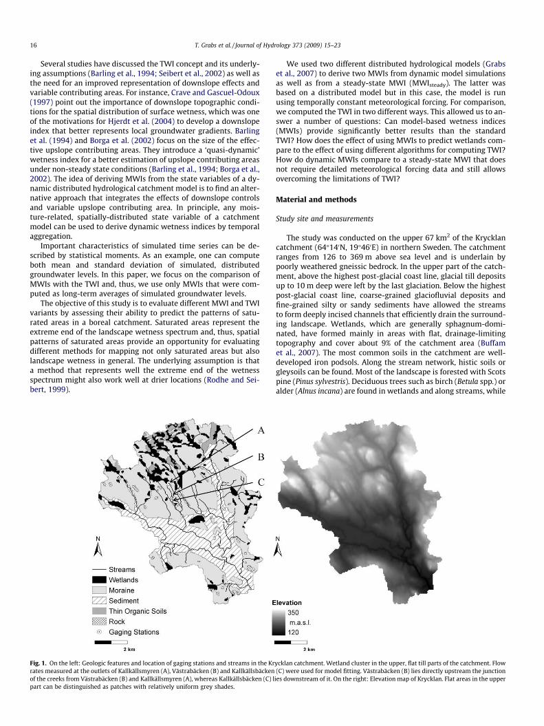
Fig. 1. On the left: Geologic features and location of gaging stations and streams in the Krrates measured at the outlets of Kallkällsmyren (A), Västrabäcken (B) and Kallkällsbäckenof the creeks from Västrabäcken (B) and Kallkällsmyren (A), whereas Kallkällsbäcken (C) lpart can be distinguished as patches with relatively uniform grey shades.

We used two different distributed hydrological models (Grabset al., 2007) to derive two MWIs from dynamic model simulationsas well as from a steady-state MWI (MWIsteady). The latter wasbased on a distributed model but in this case, the model is runusing temporally constant meteorological forcing. For comparison,we computed the TWI in two different ways. This allowed us to an-swer a number of questions: Can model-based wetness indices(MWIs) provide significantly better results than the standardTWI? How does the effect of using MWIs to predict wetlands com-pare to the effect of using different algorithms for computing TWI?How do dynamic MWIs compare to a steady-state MWI that doesnot require detailed meteorological forcing data and still allowsovercoming the limitations of TWI?

Material and methods

Study site and measurements

The study was conducted on the upper 67 km2 of the Krycklancatchment (64�140N, 19�460E) in northern Sweden. The catchmentranges from 126 to 369 m above sea level and is underlain bypoorly weathered gneissic bedrock. In the upper part of the catch-ment, above the highest post-glacial coast line, glacial till depositsup to 10 m deep were left by the last glaciation. Below the highestpost-glacial coast line, coarse-grained glaciofluvial deposits andfine-grained silty or sandy sediments have allowed the streamsto form deeply incised channels that efficiently drain the surround-ing landscape. Wetlands, which are generally sphagnum-domi-nated, have formed mainly in areas with flat, drainage-limitingtopography and cover about 9% of the catchment area (Buffamet al., 2007). The most common soils in the catchment are well-developed iron podsols. Along the stream network, histic soils orgleysoils can be found. Most of the landscape is forested with Scotspine (Pinus sylvestris). Deciduous trees such as birch (Betula spp.) oralder (Alnus incana) are found in wetlands and along streams, while

ycklan catchment. Wetland cluster in the upper, flat till parts of the catchment. Flow(C) were used for model fitting. Västrabäcken (B) lies directly upstream the junction

ies downstream of it. On the right: Elevation map of Krycklan. Flat areas in the upper

T. Grabs et al. / Journal of Hydrology 373 (2009) 15–23 17

spruce trees (Picea abis) usually grow in the transition zones be-tween riparian soils and podsols. For forestry purposes, many smallstreams were deepened and additional ditches built during the lastcentury to improve soil drainage. The forest became a researcharea in 1923; a field station and gauging station were built in1979 when expanded climate measurements were started. Streamflow, soil hydraulic properties as well as water table and soil mois-ture variations have been monitored in the 0.5 km2 Kallkällsbäckensub-catchment since 1980 (Bishop et al., 1990; Kohler et al., 2008).Stream flow is also monitored at two internal gaging stations ofKallkällsbäcken (Fig. 1), Västrabäcken and Kallkällsmyren.Västrabäcken is completely covered by forest, while Kallkällsmy-ren and Kallkällsbäcken are forested mixed with 40% and 15% wet-lands, respectively.

Annual precipitation averages 600 mm, and the annual mean airtemperature is 1 �C. Approximately one third of the annual precip-itation falls as snow (Ottosson Löfvenius et al., 2003) and there areon average 172 days of snow cover before spring runoff begins inApril or May.

The spatial distribution of wetlands was determined from aquaternary deposits coverage map (1:100,000, Geological Surveyof Sweden, Uppsala, Sweden) (Fig. 1). Laudon et al. (2007) com-pared areas marked as peat in the quaternary deposits coveragemap with areas marked as wetlands in a land cover map(1:12,500, Lantmäteriet, Gävle, Sweden) and found that the areaswere almost identical and highly correlated (r2 = 0.98,p < 0.0001). A few small lakes surrounded by wetlands were alsoclassified as saturated areas. These areas are predominantly pres-ent in the upper, flat till part of the catchment.

Wetness indices

The wetness indices used in this study are based on theassumption that surface topography is the main controlling factorof groundwater table depths and flowpaths. In many cases, otherfactors such as subsurface topography (Freer et al., 1997) or hydro-geological characteristics of the aquifer (Haitjema and Mitchell-Bruker, 2005) also need to be considered. In the studied catchment,the basic prerequisites for relating groundwater levels to topogra-phy are fulfilled for the upper, moraine part of the catchment. Inthe lower, sedimentary part surface topography is a less importantfactor due to the hydrogeological characteristics. Therefore, the lat-ter area was excluded from the analysis in this paper. For the upperpart of the catchment (68% of the entire catchment area), five dif-ferent wetness indices were calculated and compared to mappedwetlands. Three of these indices, the MWIs, were derived fromtwo distributed hydrological models while the other two representdifferent variants for calculating the TWI (Fig. 2).

The simulations for generating the MWIs are based on two spa-tially distributed versions of the conceptual HBV model (Bergs-tröm, 1976, 1995) using a 50 m � 50 m raster. In this model, the

Fig. 2. Overview over the di

computations are performed for grid cells, and lateral groundwaterflow is computed based on local, time-variant gradients. Both ver-sions compute lateral flows based on Darcy’s law using hydraulicgradients, which is a pre-requisite for this study. The first versionrelies on the traditional HBV concept, while the second is a modi-fied version of the HBV model where saturated and unsaturatedsoil storages are coupled (Seibert and McDonnell, 2002; Seibertet al., 2003). The coupling of these storages allows a more realisticsimulation of water tables and soil moisture in wetlands or at otherlocations characterized by near-surface groundwater.

Both models were calibrated against discharge data for the per-iod from 6 April 2003 to 30 September 2004 for two subcatch-ments of Kallkällsbäcken (Fig. 1) and compared against flowmeasured at the outlet of Kallkällsbäcken (Grabs et al., 2007). Allmodel simulations relied on spatially uniform parameters and in-puts. Temperature and precipitation inputs were also adjusted tochanges in elevation using lapse rates (�0.6 �C/100 m for temper-ature and +10%/100 m for precipitation). Spatial variations of sim-ulated groundwater storages were thus solely controlled bytopography. After calibration, the models were applied to the en-tire Krycklan catchment, and the model simulations of spatiallydistributed values were used to derive MWIs. The derived MWIswere only evaluated in portions of the catchment that are similarin terms of till and wetland coverage to the subcatchments usedfor calibration. The hydrologically dissimilar sedimentary portionsof the catchment were excluded from the analysis. There are sev-eral possibilities to aggregate the time series into a single valuefor each grid cell. In this study, the MWIs were calculated as nor-malized annual average values of simulated water storage in thesaturated zone of the soil column.

The MWI derived from the distributed HBV model is termedMWIhbv, while the MWI derived from the modified distributedHBV model is termed MWImod. Furthermore, a steady-state wet-ness index (MWIsteady) was computed by applying a constant netrainfall rate of 1 mm per day to the calibrated version of the mod-ified HBV model. Unlike the TWI, the MWIsteady does not rely on theassumption that groundwater flow exactly follows the surfacetopography. In comparison with the MWIs, the conceptualizationof the coupling of the saturated and unsaturated zones does notinfluence the result since, at steady state, there is no dynamicinteraction between these zones (i.e., groundwater levels are con-stant in time). Most importantly, the MWIsteady is derived from amodel in steady-state and has no time-varying component. Hence,the comparison of the MWIsteady to the other indices distinguishesthe importance of downslope controls from the benefit of runningthe model with temporally varying forcing data.

For comparison, we also computed the TWI values. The TWI at acertain point in the catchment is defined as the upslope area perunit contour length, as, divided by the local gradient, tan b (Eq. (1)).

TWI ¼ lnðas= tanðbÞÞ ð1Þ

fferent wetness indices.

18 T. Grabs et al. / Journal of Hydrology 373 (2009) 15–23

There are different algorithms to compute TWI distributions(Sørensen and Seibert, 2007). In this study, we applied the widelyused multidirectional flow algorithm as proposed by Quinn et al.(1991) (TWIMD8), and a new flow algorithm which was recentlysuggested by Seibert and McGlynn (2007) (TWIMD1). The latteralgorithm is an extension of the method of Tarboton (1997) anduses triangular facets to calculate the downslope routing of theaccumulated area. In addition, for computing TWIMD1, the localgradients, tan b, were replaced by the downslope index suggestedby Hjerdt et al. (2004) as a better approximation of local ground-water gradients.

Evaluation of wetness indices

In this study, we evaluated the performance of the differentwetness indices based on their capability to predict the spatial dis-tributions of wetlands. It is important to recognize that spatiallyuniform parameterizations were used. Therefore, the predicteddistribution of wetlands is not caused by spatially varying param-

Fig. 3. Maps with normalized values of TWI and MWI indices. Areas that are pred

eters but is an emerging property of the model simulation and af-fected only by topography. The similarity between observedwetlands and patterns produced by the various wetness indices(Figs. 2 and 3) was quantified using different statistical measures.The objective of this comparison was to assess the capacity ofthe indices to predict the geographic position of the wetland andtheir ability to generate a clear contrast between wetland and sur-rounding areas as well as their capacity to reproduce the landscapetopology of the observed wetlands. Prior to these analyses, thewetness index maps were reclassified into binary maps (‘wetland’,‘no wetland’). Specific threshold values were used for this reclassi-fication. The threshold was chosen so that the estimated wetlandpercentage equaled the percentage of observed wetlands. As men-tioned before, the sedimentary zones of the catchment were ex-cluded, which reduced the actual study area from 67 km2 to47.4 km2, of which 13.4% was wetland. Each grid cell for whichthe wetness index value belonged to the highest 13.4% values ofthe distribution is assigned a value of 1 (‘wetland’), all other gridcells were set to 0 (‘no wetland’) (Fig. 3).

icted to be wet are dark, while light areas are predicted to be relatively dry.

Table 1Confusion matrix showing the number of agreements (yes–yes, a; no–no, d) anddisagreement (yes–no, c; no–yes, b) for predicted (Wpredicted) and observed wetlands(Wobserved).

Wpredicted

Yes No

Wobserved

Yes a bNo c d

Table 2An overview of the applied similarity coefficients and their theoretical range.Negative values of Cohen’s kappa k indicate that the observed spatial agreement isless than the spatial agreement that a random predictor would achieve. In practice,however, one usually expects j to fall in the interval between zero and one. Thecoefficients refer t, the quadrants of the confusion matrix (Table 1), and the variable‘‘m”, the total number of grid cells, i.e. m = a + b + c + d.

Coefficient Expression Range

SC (spatial coincidence) aaþb [0, 1]

SM (simple matching) aþdm [0, 1]

j (Cohen’s kappa) ðaþdÞ�ðaþdÞm�ðaþdÞ

[�1, 1]

Table 3Quantitative performance measures describing the fit between predicted andobserved wetlands. Higher values indicate a better performance. The rank of thedifferent wetness indicators is established by arranging all performance measures indecreasing order. SC is the percentage of correctly predicted wetlands relative to thetotally observed wetlands, SM is the simple matching coefficient and k is the kappacoefficient of agreement.

Rank SC SM j

MWImod 1 0.56 0.88 0.49MWIsteady 2 0.53 0.87 0.46MWIhbv 3 0.52 0.87 0.44TWIMD1 4 0.50 0.87 0.42TWIMD8 5 0.49 0.86 0.41

Table 4Significance of the pairwise comparison of j-scores achieved by different dynamicand topographic wetness indices. Cases where the alternative hypothesis H1:jrow > jcolumn is supported with a confidence level of 95% are marked with a ‘‘+”.Cases where the higher ranked index (first column) does not perform significantlybetter than the lower ranked index (first row) are marked with a ‘‘0”. For example, theMWIhbv index (line 3) does not perform significantly better than the TWIMD1 index(column 3) even though the j-score of MWIhbv is higher than the j-score of theTWIMD1 index.

MWIsteady MWIhbv TWIMD1 TWIMD8

MWImod + + + +MWIsteady 0 + +MWIhbv 0 +TWIMD1 0

T. Grabs et al. / Journal of Hydrology 373 (2009) 15–23 19

There is no generally accepted, single method to compare rastermaps with binary data. Wealands et al. (2005) provide a review ofdifferent approaches for comparing spatial patterns. In this study,we evaluated the various indices using three similarity coefficientscomprising a measure of direct spatial coincidence (SC), the sim-ple-matching coefficient (SM) and Cohen’s kappa statistic of agree-ment (j) (Table 2). These indices represent different ways ofweighing spatial agreement and disagreement when comparingraster maps cell-by-cell. The results of the cell-by-cell comparisonare summarized in a confusion matrix (Table 1), which providesthe basis for the calculation of the similarity coefficients Althoughwe consider j to be the most suitable measure, the SC and SM coef-ficients are also presented because these were already used,although under different names, in previous studies (Creed et al.,2003; Dahlke et al., 2005; Güntner et al., 2004; Rodhe and Seibert,1999).

It is noteworthy that in contrast to all other measures, Cohen’skappa (j) also accounts for the part of the agreement due tochance, i.e. the part of agreement that could be achieved by anyrandom predictor. The chance-correction is accomplished by sub-tracting the expected agreement, (aþ d) (Eq. (2)), from the actualagreement, (a + d). The calculation of actual and expected agree-ment is based on coefficients from the confusion matrix (Table 1).

ðaþ dÞ ¼ aþ bm� ðaþ cÞ þ bþ d

m� ðc þ dÞ ð2Þ

The j-scores were also compared pairwise to test whether twowetness indices differ significantly (Sheskin, 2003). In practice, thisallows for a more objective judgment about the actual rankingeven in cases where two wetness indices have very similar j-scores.

The Kolmogorov–Smirnov measure (dKS) can be used to assessthe capacity of different wetness indices to separate wetlands fromsurrounding non-wetland areas (Rodhe and Seibert, 1999). Unlikethe previous indices, the dKS is a global performance measure thatdoes not involve spatial aspects. The dKS represents the maximaldistance between two empirical cumulative distribution functions(ECDFs) (Sheskin, 2003). The first ECDF contains only wetness in-dex values from observed wetlands, whereas the second ECDF con-tains wetness index values from all other areas. For two identicalECDFs the dKS is zero; for two completely non-overlapping ECDFsthe dKS value equals one. The idea behind this is that a good wet-ness index separates wetlands from surrounding non-wetlandareas more clearly than a bad wetness index. Given an ideal mapof observed wetlands and a perfect wetness index, the value ofdKS would be one.

Wetlands and lakes are distinct landscape units that might havean important influence on stream chemistry as well as on land-scape and stream ecology. Topological aspects such as fragmenta-tion, size and proximity determine, to a large degree, the actualinteraction between saturated areas and other landscape elements.Thus, it is important to know how well different wetness indicesare able reproduce the observed landscape structure. In this study,we used the freely available FRAGSTAT software package (McGari-gal and Marks, 1995) to calculate the total number of individual

patches, N, as well as the area-weighted means of patch area,Aa-w (Eqs. (3) and (4)). Grid cells were considered to belong tothe same individual patch when they were neighboring in one ofthe four cardinal directions, while grid cells only connected in adiagonal direction were considered to belong to different patches.

ðiÞ Aa-w ¼XN

i¼1

xi � Ai ð3Þ

ðiiÞ xi ¼AiPNi¼1Ai

ð4Þ

Results

The different indices corresponded to varying degrees with theobserved wetlands. The general ranking of the wetness indices wasthe same regardless of the chosen similarity coefficient (Table 3).This result could be expected because all the coefficients are de-rived from similar quantities (Tables 1 and 2).

The indices achieved SC and SM scores that compare well withsimilar studies (Creed et al., 2003; Dahlke et al., 2005; Güntneret al., 2004; Rodhe and Seibert, 1999). The MWI variants were inbetter agreement with the observed wetlands than the TWI. Of

Table 5Values of the Kolmogorov–Smirnov D (dks) statistic describing how clearly an indexseparates wetlands from non-wetlands.

MWImod MWIsteady MWIhbv TWIMD8 TWIMD1

dKS 0.58 0.58 0.54 0.52 0.51

Table 6Results of the landscape structure analysis performed with the FRAGSTAT software.The table shows the total number of distinct wetland patches, N, as well as the area-weighted means of the patch-size, Aa-w.

N Aa-w (ha)

Wetlands 157 23.0MWImod 292 30.3MWIsteady 328 16.6MWIhbv 329 15.4TWIMD1 565 4.7TWIMD8 592 11.4

20 T. Grabs et al. / Journal of Hydrology 373 (2009) 15–23

the MWI indices, the dynamic index based on the modifieddistributed HBV model (MWImod) performed best, the steady-stateMWIsteady index was the second best, followed by the dynamicindex based on the distributed HBV model (MWIhbv).

The j-scores were used to test whether the scores from a pair ofwetness indices differ significantly (Sheskin, 2003). A test scorewas calculated for every possible combination of two wetness indi-ces and then compared to the 0.05 standard z-scores (Table 4).MWImod, which was the highest ranked index, was found to have

Fig. 4. Maps with observed and predicted saturated areas. Saturated areas are shadedvalue‘0’). The first map shows the location of the observed saturated areas, while the otappear visually more similar to the observed saturated areas than the more fragmented

a significantly higher j-score than all other indices. TWIMD1 andTWIMD8 did not perform as well. Based on the analysis in thisstudy, the different approaches to compute TWI did not providesignificantly different results.

Evaluating the discriminatory strength of the indices using thedKS statistic resulted in largely the same ranking of the wetness

black (‘wetland’, value ‘1’) and not-saturated areas are shaded grey (‘no wetland’,her maps show the position of the predicted saturated areas. The MWI predictionsTWI predictions.

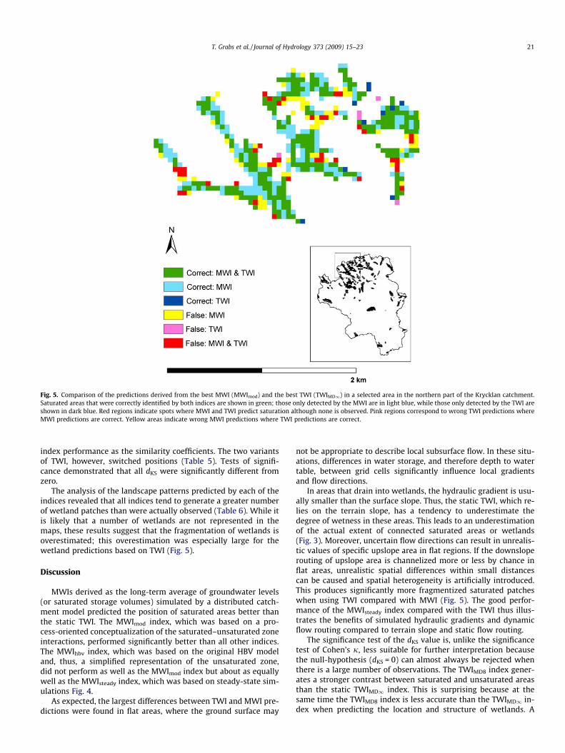
Fig. 5. Comparison of the predictions derived from the best MWI (MWImod) and the best TWI (TWIMD1) in a selected area in the northern part of the Krycklan catchment.Saturated areas that were correctly identified by both indices are shown in green; those only detected by the MWI are in light blue, while those only detected by the TWI areshown in dark blue. Red regions indicate spots where MWI and TWI predict saturation although none is observed. Pink regions correspond to wrong TWI predictions whereMWI predictions are correct. Yellow areas indicate wrong MWI predictions where TWI predictions are correct.

T. Grabs et al. / Journal of Hydrology 373 (2009) 15–23 21

index performance as the similarity coefficients. The two variantsof TWI, however, switched positions (Table 5). Tests of signifi-cance demonstrated that all dKS were significantly different fromzero.

The analysis of the landscape patterns predicted by each of theindices revealed that all indices tend to generate a greater numberof wetland patches than were actually observed (Table 6). While itis likely that a number of wetlands are not represented in themaps, these results suggest that the fragmentation of wetlands isoverestimated; this overestimation was especially large for thewetland predictions based on TWI (Fig. 5).

Discussion

MWIs derived as the long-term average of groundwater levels(or saturated storage volumes) simulated by a distributed catch-ment model predicted the position of saturated areas better thanthe static TWI. The MWImod index, which was based on a pro-cess-oriented conceptualization of the saturated–unsaturated zoneinteractions, performed significantly better than all other indices.The MWIhbv index, which was based on the original HBV modeland, thus, a simplified representation of the unsaturated zone,did not perform as well as the MWImod index but about as equallywell as the MWIsteady index, which was based on steady-state sim-ulations Fig. 4.

As expected, the largest differences between TWI and MWI pre-dictions were found in flat areas, where the ground surface may

not be appropriate to describe local subsurface flow. In these situ-ations, differences in water storage, and therefore depth to watertable, between grid cells significantly influence local gradientsand flow directions.

In areas that drain into wetlands, the hydraulic gradient is usu-ally smaller than the surface slope. Thus, the static TWI, which re-lies on the terrain slope, has a tendency to underestimate thedegree of wetness in these areas. This leads to an underestimationof the actual extent of connected saturated areas or wetlands(Fig. 3). Moreover, uncertain flow directions can result in unrealis-tic values of specific upslope area in flat regions. If the downsloperouting of upslope area is channelized more or less by chance inflat areas, unrealistic spatial differences within small distancescan be caused and spatial heterogeneity is artificially introduced.This produces significantly more fragmentized saturated patcheswhen using TWI compared with MWI (Fig. 5). The good perfor-mance of the MWIsteady index compared with the TWI thus illus-trates the benefits of simulated hydraulic gradients and dynamicflow routing compared to terrain slope and static flow routing.

The significance test of the dKS value is, unlike the significancetest of Cohen’s j, less suitable for further interpretation becausethe null-hypothesis (dKS = 0) can almost always be rejected whenthere is a large number of observations. The TWIMD8 index gener-ates a stronger contrast between saturated and unsaturated areasthan the static TWIMD1 index. This is surprising because at thesame time the TWIMD8 index is less accurate than the TWIMD1 in-dex when predicting the location and structure of wetlands. A

22 T. Grabs et al. / Journal of Hydrology 373 (2009) 15–23

higher discriminatory strength of an index therefore does not im-ply good performance according to the other tested quality mea-sures. For these reasons the dKS statistic, although used in aprevious study (Rodhe and Seibert, 1999), does not seem to be asuitable measure in this type of application.

The size and number of landscape elements are topologicalmeasures and therefore useful to assess the performance of thewetness indices in a different way compared to the previously de-scribed performance measures. As discussed earlier, the static TWIhad a tendency to underestimate the extent and contiguity of wet-lands. This resulted in smaller and more fragmented wetlandpatches, i.e., the average area, Aa-w, was smaller and the numberof wetland patches, N, was larger. Based on these rather clear re-sults, one can assume that other pattern measures, which mightbe more appropriate in other applications, would also be affectedby the limitations of most indices to reproduce the observed land-scape patterns.

Topographic indices depend on the quality and resolution of theDEM from which they were derived (Beven, 1997; Sørensen andSeibert, 2007), while benchmarking their ability to reproduce ob-served wetland patterns is clearly influenced by the accuracy andcompleteness of the observed wetlands used for benchmarking(Creed et al., 2003). Hence, it is likely that better input data wouldaffect the performances of the wetness indices but it remains diffi-cult to predict in which way the results would change. For example,an increased resolution of the DEM does not necessarily lead to bet-ter performance because groundwater flow is less likely to followsmall-scale topography. The traditional TWI is, theoretically, moresensitive to scale-effects than the MWIs that account for downslopecontrols. Particularly at high resolutions, micro-topographic fea-tures can lead to highly variable terrain slope values, which areunrealistic estimates of hydraulic gradients. Such features will besmoothed out by calculating groundwater storages and hydraulicgradients between grid cells. The choice of a MWI instead of theTWI is therefore attractive when working with high-resolutiondata, but it also requires considerably more computer resources.

The main questions addressed in this study do not depend onthe absolute performances of the indices but rather on their rank-ing. It is therefore crucial to assess the robustness of the estab-lished ranking. The pairwise comparison of the j-scores (Table 4)allows such a qualitative assessment of the robustness of the rank-ing. Pairs of indices with significantly different j-scores are lesslikely to switch their position than pairs whose j-scores are notsignificantly different.

The choices in the conceptualization of hydrological processgreatly influence the derived model-based wetness indices. TheMWI maps are dependent on the catchment model (including itsparameterization) used to simulate the spatially distributed statevariables. The differences between the MWImod and MWIhbv indi-ces indicate the effect of using different models. However, bothindices and the steady-state MWIsteady index performed consider-ably better than the TWI. Linking the TWI to spatial patterns ofwetness implicates a simplified conceptualization of hydrologicalprocesses, which, as shown here, can significantly influence the re-sults. Replacing the TWI concept with a distributed hydrologicalmodel is therefore a tradeoff between process representation andparameter parsimony. We believe that relatively simple, concep-tual, distributed models, similar to the ones used in this study,are a good compromise between these two opposing goals.

Conclusions

The different topography-based indices were evaluated basedon their ability to predict observed wetlands. For the TWI, thesepredictions were directly derived from topography, whereas for

MWIs these predictions were derived from spatial variationscaused only by topography. In other words, the spatial distributionof predicted wetland was an emerging feature rather than an effectof a spatially varying parameterization. The various indices wereable to predict the distribution of observed wetlands althoughthere were clear differences in performance. The model-basedMWIs generally outperformed the TWI. In addition, the steady-state wetness index (MWIsteady) that, unlike the other MWIs, doesnot require detailed meteorological input data performed betterthan the TWI.

While this paper focuses on the comparison of MWIs with theTWI and, thus, uses only long-term averages of the distributedmodel simulations, we wish to emphasize the potential to deriveother indices using different ways of temporal aggregation of themodel simulations. Measures such as the standard deviation, meanvalues during shorter periods, or change rates might provide usefulinformation. The index approach allows capturing essential spatialcharacteristics in a more efficient way than using model simula-tions directly. In this study, we demonstrated that the applicationof a catchment model allows better use of topographic data thanthe static TWI. These results encourage further work on model-based indices to describe spatially variable hydrologic conditions.

References

Ågren, A., Buffam, I., Jansson, M., Laudon, H., 2007. Importance of seasonality andsmall streams for the landscape regulation of DOC export. Journal ofGeophysical Research G: Biogeosciences 112, G03003. doi:10.1029/2006JG000381.

Barling, R.D., Moore, I.D., Grayson, R.B., 1994. A quasi-dynamic wetness index forcharacterizing the spatial distribution of zones of surface saturation and soilwater content. Water Resources Research 30 (4), 1029–1044.

Bergström, S., 1976. Development and application of a conceptual runoff model forScandinavian catchments. Department of Water Resources Engineering, LundInstitute of Technology, University of Lund.

Bergström, S., 1995. The HBV model. Computer Models of Watershed Hydrology443, 476.

Beven, K., 1997. TOPMODEL: a critique. Hydrological Processes 11 (9), 1069–1085.Beven, K., Kirkby, M., 1979. A physically based, variable contributing area model of

basin hydrology. Hydrological Sciences Bulletin 24 (1).Bishop, K.H., Grip, H., O’Neill, A., 1990. The origins of acid runoff in a hillslope during

storm events. Journal of Hydrology (Amsterdam) 116 (1), 35–61.Borga, M., Dalla Fontana, G., Cazorzi, F., 2002. Analysis of topographic and climatic

control on rainfall-triggered shallow landsliding using a quasi-dynamic wetnessindex. Journal of Hydrology 268 (1–4), 56–71.

Buffam, I., Laudon, H., Temnerud, J., Mörth, C.M., Bishop, K., 2007. Landscape-scalevariability of acidity and dissolved organic carbon during spring flood in aboreal stream network. Journal of Geophysical Research 112, G01022.doi:10.1029/2006JG000218.

Cory, N., Buffam, I., Laudon, H., Köhler, S., Bishop, K., 2006. Landscape control ofstream water aluminum in a boreal catchment during spring flood.Environmental Science & Technology 40 (11), 3494–3500.

Crave, A., Gascuel-Odoux, C., 1997. The influence of topography on time and spacedistribution of soil surface water content. Hydrological Processes 11 (2), 203–210.

Creed, I.F., Sanford, S.E., Beall, F.D., Molot, L.A., Dillon, P.J., 2003. Cryptic wetlands:integrating hidden wetlands in regression models of the export of dissolvedorganic carbon from forested landscapes. Hydrological Processes 17 (18), 3629–3648.

Dahlke, H., Helmschrot, J., Behrens, T., 2005. A GIS-based terrain analyses approachfor inventory of wetland in the semi-arid headwaters of the Umzimvubu basin,South Africa. Remote Sensing and GIS for Environmental Studies, GöttingerGeographische Abhandlungen 113, 78–86.

Freer, J. et al., 1997. Topographic controls on subsurface storm flow at the hillslopescale for two hydrologically distinct small catchments. Hydrological Processes11 (9), 1347–1352.

Grabs, T., Seibert, J., Laudon, H., 2007. Distributed runoff modelling. Wetland runoffand its importance for spring-flood predictions. Elforsk rapport 07:16, Svenskaelföretagens forsknings-och utvecklings-Elforsk-AB, Elforsk AB, 101 53Stockholm.

Güntner, A., Seibert, J., Uhlenbrook, S., 2004. Modeling spatial patterns of saturatedareas: an evaluation of different terrain indices. Water Resources Research 40(5), W05114.

Haitjema, H.M., Mitchell-Bruker, S., 2005. Are water tables a subdued replica of thetopography? Ground Water 43 (6), 781–786.

Hjerdt, K.N., McDonnell, J.J., Seibert, J., Rodhe, A., 2004. A new topographic index toquantify downslope controls on local drainage. Water Resources Research 40(5), W05602.

T. Grabs et al. / Journal of Hydrology 373 (2009) 15–23 23

Houser, P.R. et al., 1998. Integration of Soil Moisture Remote Sensing andHydrologic Modeling Using Data Assimilation.

Koehler, S.J., Buffam, I., Laudon, H., Bishop, K., 2008. Climate’s control of intra-annual and interannual variability of total organic carbon concentration andflux in two contrasting boreal landscape elements. Geophysical Research-Biogeosciences, 113, G03012, doi:10.1029/2007JG000629.

Laudon, H., Sjöblom, V., Buffam, I., Seibert, J., Mörth, M., 2007. The role of catchmentscale and landscape characteristics for runoff generation of boreal streams.Journal of Hydrology 344 (3–4), 198–209.

McGarigal, K., Marks, B.J., 1995. FRAGSTATS: Spatial Pattern Analysis Program forQuantifying Landscape Structure. US Department of Agriculture, Forest Service,Pacific Northwest Research Station, Portland, OR.

Nilsson, M., Sagerfors, J., Buffam, I., Laudon, H., Eriksson, T., Grelle, A., Klemedtsson,L., Weslien, P., Linderoth, A., 2008. A. Complete carbon budgets for two years ofa boreal oligotrophic minerogenic mire. Global Change Biology 14 (1–6), doi:10.1111/j.1365-2486.2008.01654.x.

Ottosson Löfvenius, M., Kluge, M., Lundmark, T., 2003. Snow and soil frost depth intwo types of shelterwood and a clear-cut area. Scandinavian Journal of ForestResearch 18 (1), 54–63.

Petrin, Z., McKie, B., Buffam, I., Laudon, H., Malmqvist, B., 2007. Landscape-controlled chemistry variation affects communities and ecosystem function inheadwater streams. Canadian Journal of Fisheries and Aquatic Sciences 64 (11),1563–1572.

Quinn, P., Beven, K., Chevallier, P., Planchon, O., 1991. The prediction of hillslopeflow paths for distributed hydrological modelling using digital terrain models.Hydrological Processes 5 (1), 59–79.

Rodhe, A., Seibert, J., 1999. Wetland occurrence in relation to topography: a test oftopographic indices as moisture indicators. Agricultural and forest meteorology98, 325–340.

Seibert, J., Bishop, K., Rodhe, A., McDonnell, J., 2002. Groundwater dynamics along ahillslope: a test of the steady state hypothesis. Water Resources Research 39 (1),1014. doi:10.1029/2002WR001404.

Seibert, J., McDonnell, J.J., 2002. On the dialog between experimentalist andmodeler in catchment hydrology: use of soft data for multicriteria modelcalibration. Water Resources Research 38 (11), 1241. doi:10.1029/2001WR000978.

Seibert, J., McGlynn, B.L., 2007. A new triangular multiple flow-directionalgorithm for computing upslope areas from gridded digital elevationmodels, Water Resources Research 43, W04501. doi:10.1029/2006WR005128.

Seibert, J., Rodhe, A., Bishop, K., 2003. Simulating interactions between saturatedand unsaturated storage in a conceptual runoff model. Hydrological Processes17 (2), 379–390.

Serrano, I., Buffam, I., Palm, D., Brännäs, E., Laudon, H., 2008. Thresholds for survivalof brown trout (Salmo trutta L.) embryos and juveniles during the spring floodacid pulse in DOC-rich streams. Transactions of the American Fisheries Society137, 1363–1377.

Sheskin, D.J., 2003. The Handbook of Parametric and Nonparametric StatisticalProcedures. Chapman & Hall/CRC.

Sørensen, R., Seibert, J., 2007. Effects of DEM resolution on the calculation oftopographical indices: TWI and its components. Journal of Hydrology 347 (1–2),79–89.

Tarboton, D.G., 1997. A new method for the determination of flow directions andupslope areas in grid digital elevation models. Water Resources Research 33 (2),309–319.

Wealands, S.R., Grayson, R.B., Walker, J.P., 2005. Quantitative comparison of spatialfields for hydrological model assessment-some promising approaches.Advances in Water Resources 28 (1), 15–32.