ELECTROMAGNETIC SCATTERING FROM A 0dMG1EU

BODY OF REVOLUTION

:by

Joseph R. Mautz

Roger F. Harringtonl

TECHNICAL REPORT TR-77-10

November 1977

DEPARTMtENT OF

ELECTRICAL A14D COMPUTER ENGINEE

SYRACUSE -UNIVERSITY

C-SYRACUSE, NEW YORK 131210

y* document b

7~~~ -_ -bi reo-0n 39

A~~i r3 el

CTROMAGNETIC SCATTERING FROM A HOMOGN

BODY OF REVOLUTION i

'I N

by

Joseph R./MautzRoger F.!Harringtoii LT IC i

JUL. 1 4 19801

TECHNICAL RPW{• 'R-77-10 /

This work was supported by the Rome Air Development Center

through the Deputy of Electronic Technology under Contract/

No. F19628-76-C-0300,'and through the Air Force Post Doctoral

Program under Contract No. F30602-75-0121.

DFPARITfENT OF /ELECTRICAL AND COMPUTER ENGINEERIN(C

SYRACUSE UNIVERS1 TY

SYRACUSE, NEW YORK 13210

ru ocumenit hcw t nR xpocjrot public reh1'x-s rind sAlo; it$distribution 1s uLmrit•;e.

I/ 4 / ; /I?•

ABSTRACT

This report considers plane--wave scattering by a homogeneous

material body of revolution. The problem is formulated in terms of

equivalent electric and magnetic currents over the surface which

defines the body. Application of the boundary conditions leads to

four simultaneous surface integral equations to be satisfied by the

two unknown equivalent currents, electric and niagaetic. The set of

four equations is reduced to a coupled pair of equations by taking

linear combinations of the original four equations. Because many

pairs of linear combinations are possible, there are many surface

integral equation formulations for the problom. Two formulations

commonly encountered in the literature are discussed and solved by

the method of moments. A general computer program for material

bodies of revolution is developed, listed, and documented. Examples

of numerical computations are given for dielectric spheres and 3

finite dielectric cylinder. The computed results for the sphere ate

compared to the exact series solution obtained by separation of

variables.

•T a

Q Qa

'I D I •-÷!Tl 15i~tCa

- d

CONTENTS

PAGE

PART ONE -- ELECTROMAGNETIC SCATTERING FROM A HOMOGENEOUS MATERIALBODY OF REVOLUTION - THEORY AND EXAMPLES --------------- i1

I. INTRODUCTION 1---------------------------------------------1

II. SURFACE INTEGRAL EQUATION FO.RIJLATION ------------------- 3

III. METHOD OF MOMENTS SOLUTION FOR A BODY OF REVOLUTION---- 11

IV. FAR FIELD MEASUREMENT AND PLANE WAVE EXCITATION--------- 14

V. EXAMPLES ---------------------------------------------- 22

VI. DISCUSSION ------------------------------------------------- 36

APPENDIX A. THE EQUIVALENCE PRINCIPLE ---- ----------- 40

APPENDIX B. PROOF THAT THE SOLUTION IS UNIQUE-43

APPENDIX C. MORE EXAMPLES-----------------------------------------------46

* PART TWO - COMPUTER PROGRAM-59

I. INTRODUCTION -------------------------------------------- 59

Il. THE SUBROUTf.INE YZ----------------------------------------*- 59

IIl. THE SUBROUTINE PLANE --------------------------------------- 68

IV. THtE SUBROUTINES DECOMP AND SOLVE---------------------------71

V. THE MAIN PROGRAM --------------------------------------------- 73

REFERENCES -------------------------------------------------------------- 83

I-"

PART ONE

ELECTROMAGNETIC SCATTERING FROM A HOMOGENEOUS MATERIAL

BODY OF REVOLUTION

THEORY AND EXAMPLE$

I. INTRODUCTION

The problem of plane-wave scattering by a homogeneous material body

of revolution is formulated in terms of equivalent electric and magnetic

currents over the body surface. Application of boundary conditions leads

to a set of four integral equations to be satisfied. Linear combinations

of these four equations lead to a coupled pair of equations to be solved.

One choice of combination constants gives the formulation described by

Poggio and Miller [1]. This formulation has been applied to material

cylinders by Chang and Harrington [21, and to material bodies of revolu-

tion by Wu [3]. We will call this choice the PMCHW formulation (formed

by the initials of the above cited investigators).

Another choice of combination constants gives the formulation

obtained by MUller [4]. This formulation has been applied to dielectric

cylinders by Solodukhov and Vasil'ev [5] and by Morita [6], and to bodies

[1] A. J. Poggio and E. K. Miller, "Integral Equation Solutions of Three-dimensional Scattering Problems," Chap. 4 of Computer Techniques forElectromagnetics, edited by R. Mittra, Pergamon Press, 1973, Equa-tion (4.17).

[2] Yu Chang and R. F. Harrington, "A Surface Formulation for CharacteristicModes of Material Bodies," Report TR-74-7, Dept. of Electrical and Com-puter Engineering, Syracuse University. Syracuse, N.Y., October 1974.

[3] T. K. Wu, "Electromagnetic Scattering from Arbitrarily-Shaped LossyDielectric Bodies," Ph.D. Dissertation, University of Mississippi, 1976.

[4] C. Miller, Foundations of the Mathematical Theory of ElectromagneticWaves, Springer-Verlag, 1969, p. 301, Equations (40)-(41). (There aresome sign errors in these equations.)

[5] V. V. Solodukhov and E. N. Vasil'ev, "Diffraction of a Plane ElectromagneticWave by a Dielectric Cylinder of Arbitrary Cross Section," Soviet Physics -Technical Physics, vol. 15, No. 1, July 1970, pp. 32-36.

[6] N. Morita, "Analysis of Scattering by a Dielectric Rectangular Cylinder by

Means of Integral Equation Formulation," Electronics and Communications in

Japan, vol. 57-B, No. 10, October 1974, pp. 72-80.

1

of revolution by Vasil'ev and Materikova [7]. We will call this choice

the MUller formulation. Conditions for the uniqueness of solutions are

established in terms of the combination constants. It is found that

solutions to both the PMCHW formulation and to MUller's formulation are

unique at all frequencies.

Numerical solutions to the coupled pair of equations are obtained by

the method of moments [8]. It is relatively easy to obtain numerical solu-

tions to these equations because the required operators are the same as those

evaluated in earlier reports [9, 10]. An exemplary computer program capable

of obtaining the solution to both the PMCHW formulation and the MUller formu-

lation is described and listed. This is a main program which uses subroutines

similar to those in [10] to compute the equivalent electric and magnetic

currents and the two principal plane scattering patterns for a loss-free

homogeneous body of revolution excited by an axially incident electromagnetic

plane wave. Computed results for the equivalent currents and principal plane

scattering patterns of a dielectric sphere whose relative dielectric constant

is four show reasonable agreement between our solution to the PMCHW formula-

tion, our solution to the MUller formulation, and the "exact" series [11]

solution in the resonance region. Computer program subroutines which calcu-

late the "exact" series solution for perfectly conducting spheres as well asfor loss-free homogeneous spheres will be described and listed in a subsequent

report.

[7] E. N. Vasil'ev and L. B. Materikova, "Excitation of Dielectric Bodies ofRevolution," Soviet Physics - Technical Physics, vol. 10, No. 10, April1966, pp. 1401-1406.

[8] R. F. Harrington, Field Computation by Moment Methods, Macmillan Co.,New York, 1968.

[9] J. R. Mautz and R. F. Harrington, "H-Field, E-Field, and Combined FieldSolutions for'Bodies of Revolution," Interim Technical Report RADC-TR-77-109, Rome Air Development Center, Griffiss Air Force Base, New York,March 1977.

[10] J. R. Mautz and R. F. Harrington, "Computer Programs for H-Field,

E-Field, and Combined Field Solutions for Bodies of Revolution,"Interim Technical Report RADC-TR-77-215, Rome Air DevelopmentCenter, Griffiss Air Force Base, New York, June 1977.

[11] R. F. Harrington, Time-Harmonic Electromagnetic Fields, McGraw-Hill

Book, Co., 1961. Section 6-9.

2

II. SURFACE INTEGRAL EQUATION FORMULATION

An electromagnetic field propagating in a homogeneous medium of

permeability pe and permittivity ce is incident on the surface S of a

homogeneous obstacle of permeability Od and permittivity Ed' The sub-

script e denotes exterior medium and the subscript d denotes diffracting

medium. We wish to calculate the scattered electromagnetic field E , H

outside S and the diffracted electromagnetic field E, H inside S in terms

of the electromagnetic field Ei, H which would exist on S in the absence

of the obstacle. This original problem is shown in Fig. I where J i, M -Ei i#

are the electric and magnetic sources of E , i and n is the unit normal

vector which points outward from S.

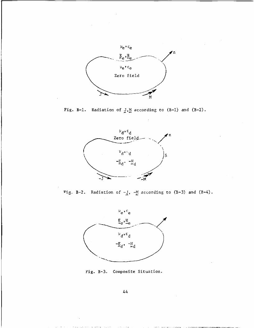
The equivalence principle (stated in Appendix A) is used to piece

together an outside situation consisting of medium p' ce and field ES, H,

outside S and an inside situation consisting of medium pe' c and field

-Ei, -H inside S. This composite situation is shown in Fig. 2. Since

E , H S is source-free outside S and E', H 1 is source-free inside S, the

only sources in Fig. 2 are the equivalent electric surface current J and

the equivalent magnetic surface current M on S.

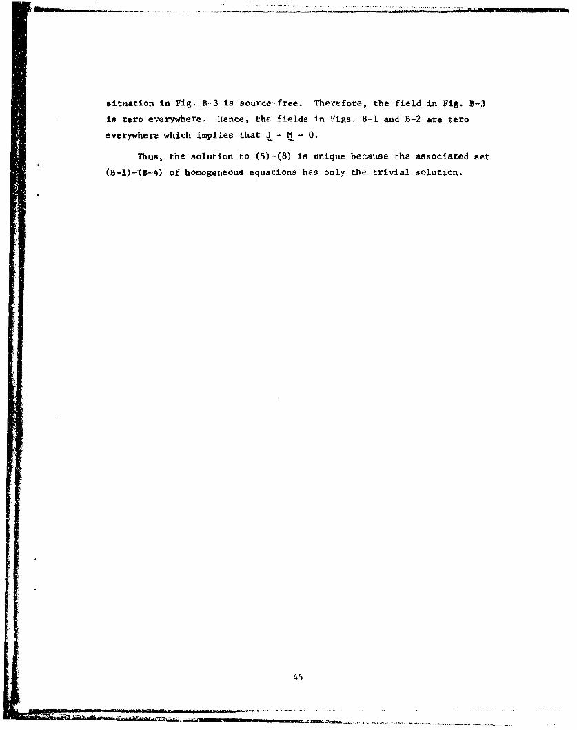
As a second application of the equivalence principle, we combine an

outside situation consisting of medium 1d' C d and zero field with an inside

situation consisting of medium Vd' Cd and field E, H. This combination of

situations is shown in Fig. 3. Since E, H is source-free inside S, the only

sources in Fig. 3 are the equivalent electric surface current -J and the

equivalent magnetic surface current -M on S. By using (A-1) and (A-2) to

express the surface currents in terms of the discontinuities of the tangen-

tial fields across S and by using

n x E n x (ES + Ei()

n x H n x (H' + (2)

on S, the interested reader can verify that the surface currents in Fig. 3

are indeed the negatives of those in Fig. 2. Equations (1) and (2) are the

boundary conditions that the tangential components of the fields in the

3

lie ,J E ,M-9

Es+ EH s+ Hn

Fig. 1. Original problem.

1ie3 e

H S

Fig. 2. Outside equivalence.

1'd' C dZero field

-14

Fig. 3. Inside equivalence.

4

original problem as shown in Fig. 1 are continuous across S.

s sThe scattered field E , H outside S and the diffracted field E, H

inside S could easily be calculated if J and M were known because the media

into which J and M radiate is homogeneous in Figs. 2 and 3. We have to

determine J and M. The equivalence principle states that there exist J and

M which radiate the fields in Figs. 2 and 3, but the equivalence principle

does not tell what J and M are. The equivalence principle does state that

J nx H (3)

M E x n (4)

but this is not very useful because E and H are unknown.

From Figs. 2 and 3,

-n xE = n x E (5)

- i-n x H = n x H (6)

^-e

+-n x E = 0 (7)

-d

-n x H =0 (8)

wihere

E is the electric field just inside S due to J, M, radiating in vee

H is the magnetic field just inside S due to J, 14, radiating in Vee

E is the electric field just outside S due to J, M, radiating in PdCd, d dd

11+ is the magnetic field just outside S due to J, M, radiating in

The equivalent currents J, M which appear in Figs. 2 and 3 satisfy (5)-(8)

because (5)-(8) were obtained from Figs. 2 and 3. It is shown in Appendix B

that the solution to (5)-(8) is unique. Therefore, (5)-(8) uniquely deter-

mine the equivalent currents J, M of Figs. 2 and 3.

Equations (5)-(8) form a set of four equations in the two unknowns

J and M. The usual methods of equation solving apply only when the number

of equations is equal to the number of unknowns. We want to reduce the

set of four equations (5)-(8) to two equations. One way to do this is to

form the linear combination

5

nx (E +ZE +) n xEi1 (9)- e ;-d -

of (5) and (7) and the linear combination

nx (H + )n xHi (10)

of (6) and (8) where a and a are complex constants.

The solution J, M to (5)-(8) satisfies (9) and (10). This J, 14

will be the only solution to the pair of equations (9) and (10) if

-n x (E +c )' O (II0

-n x (H + 8H) 0 (12)1 -.-e

have only the trivial solution J M 4 0. From (11) and (12),

Pe a$ P d (13)

where P eis the complex power flow of E e., H einside S and P dis the complex

power flow of E+,H+outside S. The asterisk in (13) denotes complex con-*:d ~

jugate. If a$ is real, then the real part of (13) reduces to

Real(P e a6 ~ Real(P d (14)

If a$ is not only real but also positive, then

Real(P d 0 (15)

because both Real(P e) and Real(P d) are greater than or equal to zero.

Equation (15) implies that

n E x H = 0 (16)-Xd - d

Substitution of (16) into (11) and (12) yields

n xE =n xH =0 (17)-e - -e

6

The system of equations (16) and (17) is precisely the homogeneous system

of equations associated with (5)-(8). It was shown in Appendix B that

this homogeneous system of equations has only the trivial solution J = M = 0.

Therefore, if cx8 is real and positive, then the coupled pair of equations(11) and (12) has only the trivial solution J = M = 0 so that the solution

J, M to (5)-(8) is the only solution to the coupled pair of equations (9)

and (10).

If a = 8 = 1, then (9) and (10) become

-n x (E E+) = n Ei (18)

x (H +) n H (19)

The set of equations (18) and (19) is the coupled pair of surface integral

equations transcribed by Poggio and ýfiller [1]. We call these equations

the PMCHW equations. Since a = = I implies that 08 is real and positive,

the argument consisting of (ll)-(17) and involving real power flow shows

that (18) and (19) uniquely determine the desired J, M of Figs. 2 and 3.

That (18) and (19) uniquely determine J, ýM of Figs. 2 and 3 can

also be shown as follows. The desired J, M of Figs. 2 and 3 satisfies

(18) and (19) because (18) and (19) were obtained from Figs. 2 and 3.

This desired J, M will be the only solution to (18) and (19) if the associ-

ated set of homogeneous equations

-( + E d) 0 (20)

-n x (H (21)

has only the trivial solution J = M = 0.

The following argument shows that (20) and (21) have only the trivial

solution J = M = 0. Let Ed, H be the electromagnetic field outside S due

to J, M radiating in P d' Ed. Let E e, H be the electromagnetic field inside_ -e

S-due to J, M radiating in V . Use the equivalence principle to formShn muedum -,Mrdaigi e' -H

the composite situation consisting of medium Pd' Cd and field E H outside

SaVe Ee and field -e -He inside S as shown in Fig. 4. In

Fig. 4, Ed, Hd is a source-free Maxwell]4 an field outside S. Since Ee, H e is

7

Ud,•d

-e -eD

Fig. 4. Composite situation used to prove that (20)and (21) have only the trivial solutionJ= M =0.

1 E,

Fig. 5. Composite situation 'i.qed Vi prove that (26)and (27) have only the tr-vial solution

J=M =0.8d

a source-free Maxwellian field inside S, the field -E , -1e appearing in

Fig. 4 is also a source-free Maxwellian field inside S. Now, (20) and (21)

state that the tangential components of the field in Fig. 4 are continuous

across S. Thus, Fig. 4 is entirely source-free so that the field in Fig. 4

is zero everywhere in which case (B-l)-(B-4) are satisfied. But, as shown in

Appendix B, (B-I)-(B-4) have only the trivial solution J = M = 0. Hence,

(20) and (21) have only the trivial solution J = M = 0.

If

S= (22)

8 - li (23)0e

then (9) and (10) become

-n x (E Cd E+ Ei (24)e

-n x (H--Hf) =nxHi (25)e

The set of equations (24) and (25) is the coupled pair of surface integral

equations obtained by MUller [4]. We call these equations the Wdller equa-

tions. The singularity that +-he kprnels of the integral equations (24)

and (25) exhibit as the source point passes through the field point is not

as pronounced as the singularity of the kernels of (18) and (19). If

lie' Ce" Ud ' and cd are real in (22)-(25), then a$ is real and positive.

In this case, the argument consisting of (1l)-(17) shows that (24) and (25)

uniquely determine the desired J, M of Figs. 2 and 3.

An alternate proof, valid for lossy media, that (24) and (25) uniquely

determine the desired J, M is presented. This proof is similar to the argu-

ment which used Fig. 4 to show that (18) and (19) uniquely determine the

desired J, M and is as follows. The desired J, M of Figs. 2 and 3 satisfies

(24) and (25) because (24) and (25) were obtained from Figs. 2 and 3. This

desired J, M will be the only solution to (24) and (25) if the associated

set of homogeneous equations

9

-n x (E -d 0 (26)-Ze -

e

-n x (H- d 0 (27)e

has only the trivial solution J M = 0.

The following argument shows that (26) and (27) have only the trivial

solution J = M =0. Let E , H be the electromagnetic field outside S dueto J, M radiating in pd, Ed. Because the electromagnetic field E, H is

to d' .i~d is

a source-free Maxwellian field in p d' Ed outside S, the dual electromagnetic

field Ed " - wherend ý' -n d

d

n d (28)d d

is also a source-free Maxwellian field outside S. Let E, H be the•e-e

electromagnetic field inside S due to J, M radiating in v e, Ce. Because

the electromagnetic field E e", H is a source-free Maxwellian field inside S,

the dual electromagnetic field ne H, 1 E wheree-e T) -e

S 4e e (29)

e

is also a source-free Maxwellian field inside S. Use the equivalence

principle to form the composite situation consisting of medium v d' Ed and

field nd H, - 1E outside S and medium ie, £e and fieldd Zd T~d -;-de

- (eH- Ee -( -I- E ) inside S as shown in Fig. 5. Now, (26) and (27)d e-e n e -e

state that the tangential components of the field in Fig. 5 are continuous

across S. Thus, Fig. 5 is entirely source-free so that the field in Fig. 5

is zero everywhere in which case (B-l)-(B-4) are satisfied. But, as shown

in Appendix B, (B-l)-(B-4) have only the trivial solution J = M = 0. Hence,

(26) and (27) have only the trivial solution J = M = 0.

10

III. METHOD OF MOMENTS SOLUTION FOR A BODY OF REVOLUTION

In this section, a method of moments solution to (9) and (10) is

developed for a homogeneous loss-free body of revolution. Special cases of

(9) and (10) are the PMCHW equations (18) and (19) and the Miller equations

(24) and (25).

For compatibility with equation (40) on page 14 of [9], we rewrite

(9) as

1 aE + E (30)- e- -e _d tan T1 -tane e

where tan denotes tangential components on S and ne is given by (29). The

fields on the left-hand sides of (30) and (10) are written as the sum of

fields due to J and fields due to M. Advantage is taken of the fact that

the operator which gives the electric field due to a magnetic current is

the negative of the operator which gives the magnetic field due to an

electric current and that the operator which gives the magnetic field due

to a magnetic current is the square of the reciprocal of the intrinsic

impedance times the operator which gives the electric field due to an

electric current. In view of the above considerations, (30) and (10) be-

come

( E (q) + L H•() -aE(J) +))t a(M)) E (31)(- e _e n1e e n e Zd nJ +me ;.:d)-tan n •e --tan

-n x (He(J) + - Ee ) + 6H(J) + E (M)) = n x Hi (32)ee -d

where E denotes the operator which gives the electric field due to an

electric current. The subscript e or d on E denotes radiation in either

le' Ce or 11d Cd" The superscript + or -, if present on E, denotes field

evaluation either just outside S or just inside S. The H's in (31) and-

(32) are the corresponding magnetic field due to electric current operators.

We stress that all E's and H's in (31) and (32) are, by definition, operators

which give electric and magnetic fields due to electric currents, even though

these operators act on both electric and magnetic currents J and M in (31)

and (32).

11

Let

CO NIjt. n n + I. nj n (33)J =- • (nj '.nj nj -nj)

n=-w j=l

O NM n=- ji j-n + nj J (34)

ehr nt I•Vt Vn n-n

where I n 1 Vt , and Vn are coefficients to be determined andnj' nj' nj nj

jt W f.(t)eJn• (35)"-ni !tJ

J fj (t)e jn (36)

In (35) and (36), t is the arc length along the generating curve of the body

body of revolution and 4 is the longitudinal angle. u and u are unit

vectors in the t and 0 directions respectively such that u x ut = n and

f (t) is the scalar function of t defined on page 10 of [9]. The body of

revolution and coordinate system are shown in Fig. 6. Substitution of

(33) and (34) into (31) and (32) yields

N + ) + t J + + +S[ (H( ) + +(HH-(J)+ (JO ())tan

n=- j=l -e nj) + - -j tan nj -e -nj ~d-j tn n

(t OL7 t(-e d E (J I E (J ='a E

ne n e nd tan nj ne (e Tid tan nJ ne -tan

(37)

O N E(Jt E ( t E J ( 0.)

-n x --(.e -nj e -d ni V t + rý -ni + e Zd-i)vO +

n=-• j 1 L e "d rd nj ne 'd nd nj

(H -(J t) + 6H + (J t))I t + (H-(JO.) + 8 + ))1MO n xHi (38)_e Znj zd -nij nj .-en -dj -i njj

Define the inner product of two vector functions on S to be the

integral over S of the dot product of these two vector functions. Because

the field operators in (37) and (38) are the same as those considered in (9],

12

only the nth term of the sum (37) or (38) contributes to the inner product

of (37) or (38) with either J-ni or J .-ni J Hence, the inner product of (37)with J-n't ,i=,2,...N, and J-n.' i=1,2,....N, successively and the inner pro-

ttwith i l2..N a -nd _ 0, i' l,2,. ..N, successively gnte inversro

duct of (38) with J -ni i=l,2,...N, and J-n i~l,2,...N, successively gives

the matrix equation

ne nd ne nd ne T1 nd ne e nd n

(_ytt - (Y - yt) (Zt + _A Zn1d) (Zn + n nne nd ne nd ne rie nd ne r- nd n

(z on e Ot) 00 + !"e ZO) (Yt + B~tt) (Yo + BYjo t:t It(Z t + nd Z d) (Zne nd nd" ne nd ne nd n n

L~ztt - Oe tt t zt )e (y ynt + t) (o + 6ýn)Vn nd ne nd nd ne nd ne rdL n

(39)

for n = 0, +1, +2 ...... .. In (39), , , and 1P are columnn n n n

vectors of the coefficients appearing in (33) and (34). Also,

(Ynf) - -ni "P n x Ufq)ds (40)

s

nf ij= - f -ni -nJ (41)

S

(p l_= jp . qEids (42)n 7i = e -ni - f n

S

Pn = L J pn x ds (43)

S

where p may be either t or 0, q may be either t or 0, and f may be

either e or d. If p=q in (40), it matters whether the magnetic field

Hf(J qj) is evaluated just outside or just inside S. The Y's without

13

carets in (39) are given by the right-hand side of (40) in which the mag-

netic field is evaluated just inside S. The Y's with carets in (39) are

given by the right-hand side of (40) with magnetic field evaluation just

outside S.

The Y and Z submatrices on the left-hand side of (39) are the same

as in equation (88) on page 24 of [9] with the reservations that the caret

on Y denotes magnetic field evaluation just outside S, and the extra sub-

script e or d denotes radiation in either e9 or v d E The I column

vectors on the right-hand side of (39) are the same as in equation (88)

on page 24 of [9] whereas the V column vectors in (39) are the same as the

V's without carets in equation (88) on page 24 of [9].

The solution V, V , I and V to the matrix equation (39) determinesn n n

the equivalent electric and magnetic currents J and M according to (33) and

(34). From Fig. 2, these currents radiate in v e' £e to produce the scattered

field outside S.

IV. FAR FIELD MEASUREMENT AND PLANE WAVE EXCITATION

In this section, measurement vectors are used to obtain the far field

of the equivalent surface currents J and M radiating in p e, £e" This far

field is the far field scattered by the homogeneous body of revolution. For

plane wave excitation, the composite vector on the right-hand side of (39)

is expressed in terms of these measurement vectors.

By -eciprocity,

E . = i (J(r)- E(IZ M(r)- H(I. ))ds (44)ES r . r rr

S

where Es is the far electric field due to J and M, It is a receiving elec-

tric dipole at the far field measurement point, E(TZr) is the electric field

due to Itr, and H(I£t -•) is the magnetic field due to It X. Both E(I2r ) and

H(I . ) are evaluated at point r on S where r is the point at which the dif-

ferential portion of surface ds is located. If £ is tangent to the radiation_r

sphere,

14

z

S

t US6

t 0

x p

Fig, 6. Body of revolution and coordinate system.

zee

ik

Z

U YI /

I I•t-".. IY

Fig. 7.Plane wave scattering by a dielectric body of

revolution.

-Jkr-jkr -jk r

(k x .Ir e •- (45)4r-Ir

Sr 411 r -T (6r

where rr is the distance between the measurement point and the origin in

the vicinity of S. Also, k is the propagation vector of the plane wave

coming from Itr, k is the propagation constant and n is the intrinsic

impedance of the medium outside S. To simplify the notation in this sec-

tion, we have omitted the subscript e from all parameters dependent on the

medium. It is understood that all far field measurement vectors and plane

wave excitation vectors depend only on the external medium p' F

Substitution of (33), (34), (45), and (46) into (44) gives

-jkrjn

,E j , e -j r r 0t _ + ý ' ' + O ~ n 4 Tr r ( R n + Rn 11 n + t •n n + ' @n n ( 4 7 )

r

for It u r and

-,jkrr -jnr

= k to_ t + RtIt - ýn n r (48)4Er (-R V RV 1 t4-t + -~ )e4-rr n.. n n n n n n n

Sr r rfor 19r = u where r and u are unit vectors in the 0 and r directions

ýr __4 ! ý4r rrespectively. As shown in Fig. 7, 0r and tr are the angular coordinates of

the receiver location at which 19 is placed. In (47) and (48), ES and E•0are the 0 and 6 components of Es, Also, Vn, V , and 'P are column

Sr r - a n' n

vectors of the coefficients appearing in (33) and (34). Furthermore, RPq iskn

a row vector whose jdh element is given by

Jl -Jn f r r -jk ri•Rq=k e [P~ * u e •ds (49)

where p may be either t or ,J) and ( may be either o or ,. In view of (35)

and (36), (49) Is the same as equation (92) on page 26 of [9]. It is

S shown in [91 that lie right-hand sIde of (49) does not depend on r"t !~16 ;

tFor plane wave incidence and expansilon functions J and given

by (35) and (36), the equivalent currents (33) and (34) and the fields (47)

and (48) have special forms. To obtain these forms, assume that the incident

electromagnetic field Ei, Hi is either a 0 polarized field defined by

Se-jkt rE= u e (50)

j -k t rH -k u e (51)S•-y

or a • polarized field defined by

-jk

(52

H kn u e (52)

' t - j k t • rHi = -t0 (53)

t

where k is the propagatiorn vector and, as shown in Fig. 7, u and u are•t •-y

unit vectors in the (t and y directions respectively. Here, 0t is the

colatitude of the direction from which the incident wave comes. k is in

the xz plane. No generality is lost by putting k in the xz plane because

if k were shifted out of the xz plane by an angle ýt' the response would

also be shifted by the same angle ýt"

Substituting (50) and (51) into (42) and (43), then substituting (52)

and (53) into (42) and (43), next taking advantage of the relationships

tJi x n J (54)

n (55)~-ni i

which are apparent from (35), (36) and Fig. 6, then comparing the results

with (49), and finally using equation (104) on page 29 of [9], we obtain

.17

nn nl n

S11 n nn

nIn n -R n

The first superscript on V nand I nin (56) is the superscript which appears

n n n~ f

on the right-hand side of (39). The second superscript on ý and I in (56)

n ndenotes the polarization of the i~ncident plane wave.. If this second super-script is 0, the e polarized field given by (50) and (51) is incident. If

this second subscript is p, the ý polarized field given by (52) and (53) is

incident. The jth element of the colurmn vector ýPq on the right-hand siden

of (56) is given by (49) with 0 replaced by 0 . Conceding that 8 does notr t rappear explicitly in (49), we really mean that 0 is replaced by et after theSrtsurface integral in (49) is evaluated. In other words, 0r is replaced by 0t

in equation (95) on page 27 of [9].

For plane wave incidence, the +n and -n terms in formulas (33) and

(34) for the equivalent currents can be combined as follows. According to

equations (1.02) and (103) of [9], the Y and Z submatrices in (39) are either

even or odd in n. The even-odd properties in n of the submatrices of the

square matrix on the left-hand side of (39) are tabulated as

+ + + -4 + - -+

K+ +:

where 4+ denotes an even ý- bbmatrix and - denotes ;w odd suhmatrix. It

follows that the submatrices of the inverse of the square matrix on the

left-hand side of (39) have e. en-odd properties in n given by

18

- + - +

.+ - + -

- + - +

From (56) and the even-odd properties of •pq given by equation (104) onpage 29 of [9] the column vectors V and I on the right-hand side of

page 2n and

(39) are either even or odd in n. The even-odd properties of the sub-

matrices on the left-hand side of (56) arc tabulated as

+ -

-.-. 4-

+ -

- +

Because of the above even-odd properties of tho square matrix on the left-

hand side of (39) and the column vector on the right-hand side of (39),

the solutions to (39) satisfy

-n n --Il -1 n n (57)

tIt - t

The first superscript on the column vectors; V and i+n in (57) is that

which appears on the colunui vectors ý and 1on the left-hand side of

(39). The second superscript ;n the column vectors in (57) denotes either

the 0 or the 4 polarized In, Ldetit plane wave. Substitution of (57), (35),

and (36) into (33) and (34) yiel0s4

19

j M(t 8 )u + 2 (EtO)!cos(ný) + 2j(filO)u sin(ný) (58)0 _t n= n

e M (o + ' 2j(fV-)u sin(ný) + 2(f6 O)acos(nd) (59)n = nn -nn|

for the 0 polarized incident wave and

J= (il 10 )u + 3 2j(ftlt)u sin(np) + 2(nd#)2,cos(ni) (60)

40

1. -- = (fiV~o)u + • 2(fV-)!-cs(ný) + 2J(fVý)u sin(ný) (61)- 0 _t n=l n

for the • polarized incident wave. In (58)-(61), f is a row vector of

the f (t). The superscript 0 or • on J or M in (58)-(61) differentiates

the equivalent currents for the 0 polarized incident wave from those for

the 0 polarizcd incident wave.

The far scattered fields (47) and (48) are specialized to the 0

polarized incident plane wave by apperding the additional subscript 0 to

Es on the left-hand sides of (47) •nd (48) and the additional superscript

O to t, V, It, and V on the right-hand sides of (47) and (48). More-

over, in view of equation (104) on page 29 of [9] and (57), the +n and -r

terms in (47) and (48) can be combined. ,f' a result, (47) and ('48) become

. l+ 2 (R•( 0 + RYI +00 4 ii r o ~ n n1 n n

+ Rt 0 tH+ R40(!0 t )cos l(n) (62)n n ni n n r) j

-r

. -... . ... .•- _ t t 4 + .lt 0 +10 2 irrt n ii i n n n

2 rr

+ flP)in(nt ) (63)n n r

for the ( polarized tncident plane wave. Similarl (47) and (48)

become-- 2 0

-j krrnl

Esw ne 'Sovt + koo~o + itlo+ ojoSi~'O(4

-jkr

ktlvt +Rt kot4I + 2+ or n=l n n

. ttn I + Rn n)cos(n• )n(65)

for the 4 polarized incident plane wave. The first subscript on Es on

the left-hand sides of (62)-(65) denotes the receiver polarization and

the second subscript on Es denotes the transmitter polarization.

The scattering cross section a is defined bypq

4wr 2 1E q2a r (66)

pq iý2

where p is either 8 or o and q is either 9 or ý. In (66), Es is a com-pq

ponent of the scattered field given by (62)-(65) and IEil is the magnitudeof the electric field of the incident plane wave. According to (50) and (52),

kni = (67)

for both polarizations so that

4Trr2 jEs 12a = r pq (68)

pq k22

Normalized versions of (68) are

a2 222

a r2rJE s2_2a Pq (70)A2 -n

where a is some characteristic length associated with the scatterer. and A is

the wavelength in the external medium.

21

V. EXAMPLES

A computer program has been written to calculate the equivalent

currents and scattering patterns for a dielectric body of revolution ex-

cited by an axially incident plane wave. This program is described and

listed in Part Two. Some computational results obtained with this program

are given in this section.

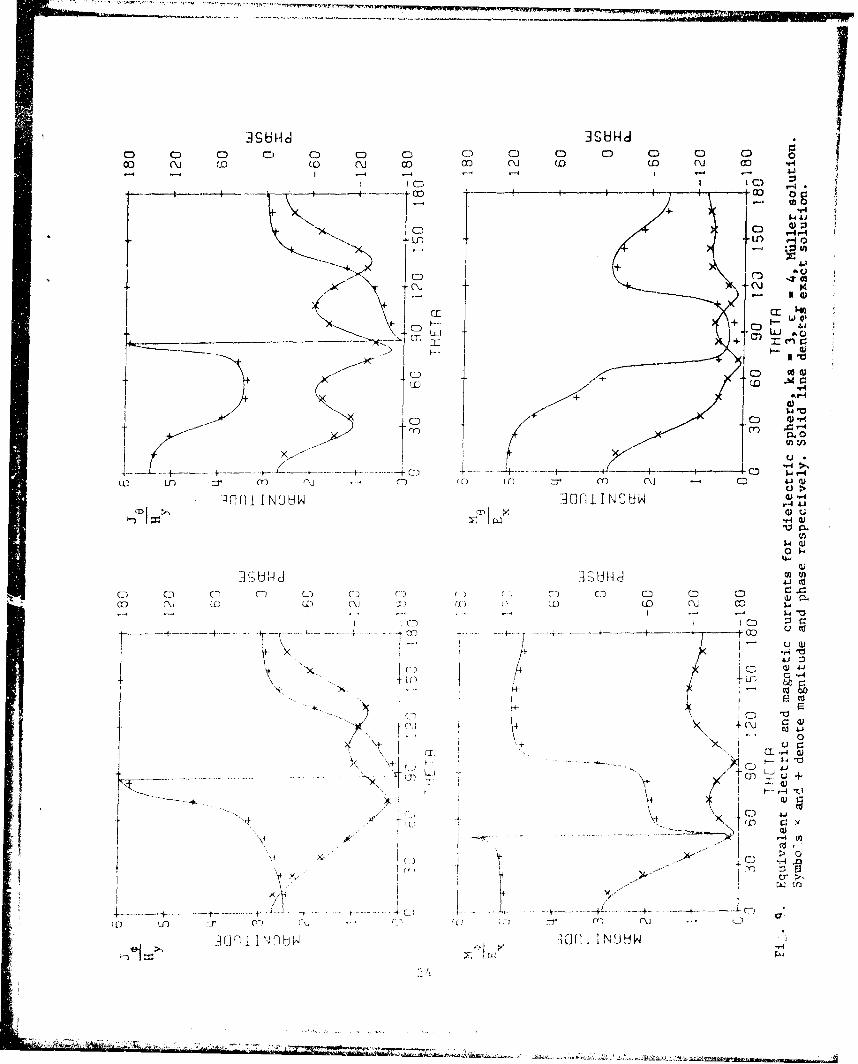
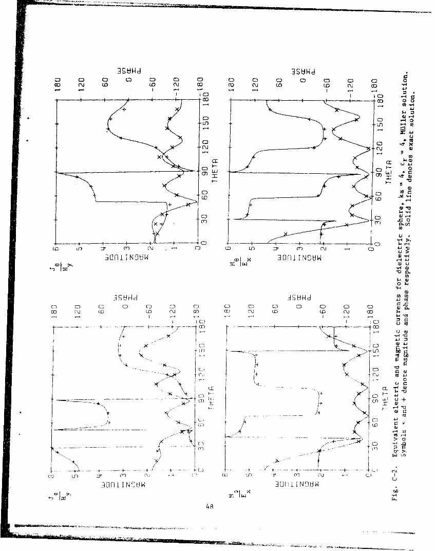
Figures 8 and 9 show the magnitude and phase of the normalizedJi M0 M

equivalent currents H -E andE on the surface of a dielectricequvalntcurens • ,H , E-- an Ey y x x

sphere for which ka = 3 and c = 4. Here, k is the propagation constant

in free space, a is the radius of the sphere and cr is the relative

dielectric constant of the sphere. Figure 8 represents our solution of the

PMCHW formulation. Figure 9 depicts our solution of the MUller formulation.

In Figs. 8 and 9, the incident field is a plane wave traveling in

the positive z direction. THETA = 0* is the forward scattering direction

and THETA = 1800 is the backscattering direction. The incident field is

given by (50) and (51) with t = 1800. The origin r = 0 is at the center

of the sphere. In Figs. 8 and 9, Ja is the u0 = - t component of electric

current (58) versus 0 in the 4 = 0 plane, J is the u component of (58)

versus 0 in the 4 = 900 plane, Me is the u8 = - component of magnetic

current (59) versus 6 in the 4 = 90* plane, and M is the u component of

(59) versus 0 in the 4 = 0* plane. For axial incidence, only the n=1 term

is present in (58) and (59). The symbols x and + denote respectively•magnitude and phase of the method of moments solution for the pertinent

component of the electric or magnetic current. The solid curves are the

exact equivalent currents obtained from the Mie series solution [11]. The

normalizing constants E and H Y are defined in terms of the incident fieldx y

(50) and (51) by

E = -u - =-knx .-X r=O

(71)H =u .H -

Hy = uY - r=O

[11] R. F. Harrington, Time-Harmonic Electromagnetic Fields, McGraw-Hill

Book Co., 1961. Section 6-9.

22

0

0 0cC C) CD.D C CD C) LI ) D rCO CU ) (flC) (0(D c

,-+------+---- 0C)IC

+

CUC) +)

4. CC)

LLJ0) I 0

C) Q. 0.0c l __vmC C r) m) cf o

>' ioi I NHW ioimuw 4 0.

C) C:) f ~ C C) C.C) CD CD 7) C) Q C) C: p I

u~

C_ I C) Ow

:ýd 4-J

+~ x~~

'X/ +

C-) / 2 CD (

LLI .;j L c

41. CD ,

C-.)co (3-40

(T) ) -T, (T) \CCC) U') 00 r (JC

2 3

CD cm CD cm) C) CD cm CD C-) 0 C) C(0N - (D Ux (00 O (0 W o P

lCD 0 C

04

I +CD C

CLi

CD + D-.

+__ m nrI I-X"

CDDcm4

(00

4CD-4Ln :11 r) ýj r)M

iririoni I NJ H ~OlO W

1,v4 Q)

14-4

:vSu{.1j V)hHM m Cr C CD UC: C) CD:1 . CD C, CD CD CD

(1) C'U 0ii ) (1. co cc

I CD 1 0 :)

U)Q CD j~

-i

)(:

t- r-4 ý

'C)E

-A~-~1 ai

'~(71

where k and n are respectively the propagation constant of free space and

the impedance of free space.

The currents of Figs. 8 and 9 were obtained by using a 20 point

Gaussian quadrature formula for all integrations in 0. All Integrations

over the functions {f (t)0 in t = a(f-8) were done by sampling each

f (t) four times. The {f (t)} consisted of 14 overlapping triangle

(divided by the cylindrical coordinate radius) functions equally spaced

in 8. More precisely,

N= 31.

NPHI - 20 (72)

MT 2

where the above variables are input data for the computer program desfxribed

and listed in Part Two, Section V.

Figures 10 and 11 show the scattering patterns radiated by the cu,'-

rents of Figs. 8 and 9 respectively. The symbols X and + denote

o a2and 2- respectively. The solid curves are the exact patterns obtained2

na Trafrom the Mie series solution [11-1. The pattcrns o00 and a,, are given by

(69), (62) and (63). Here c 0 is the 0 polarized pattern versus 0r in the

4j = 0 plane and uO is the 4 polarized pattern versus 0r in the 4 -- 90'

plane. The THETA in Figs. 10 and 11 refers to 0 . For axial incidence,r

only the n=l terms are present in (62) and (63). Elsewhere (3, 12], the

pattern C1 is called the horizontal polarization because it is polarized

parallel to the scattering plane. Similarly, the pattern o is called the

vertical polarization because it is polarized perpendicul]ar to the scatter-

ing plane.

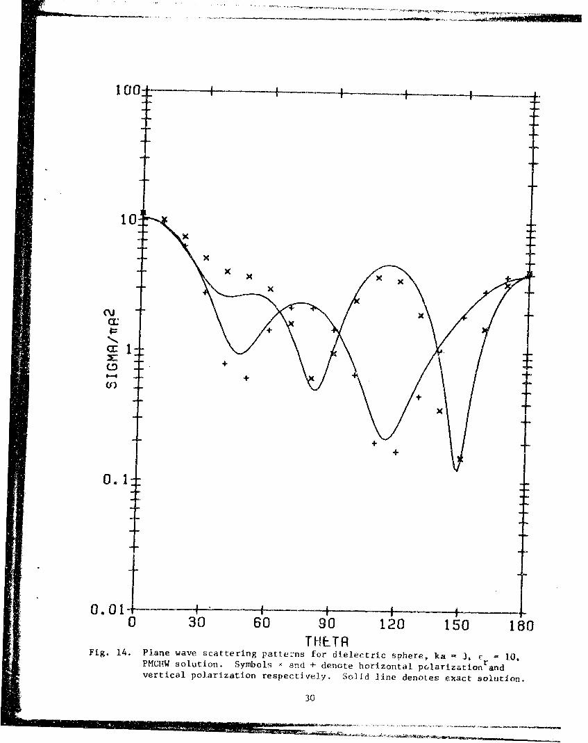
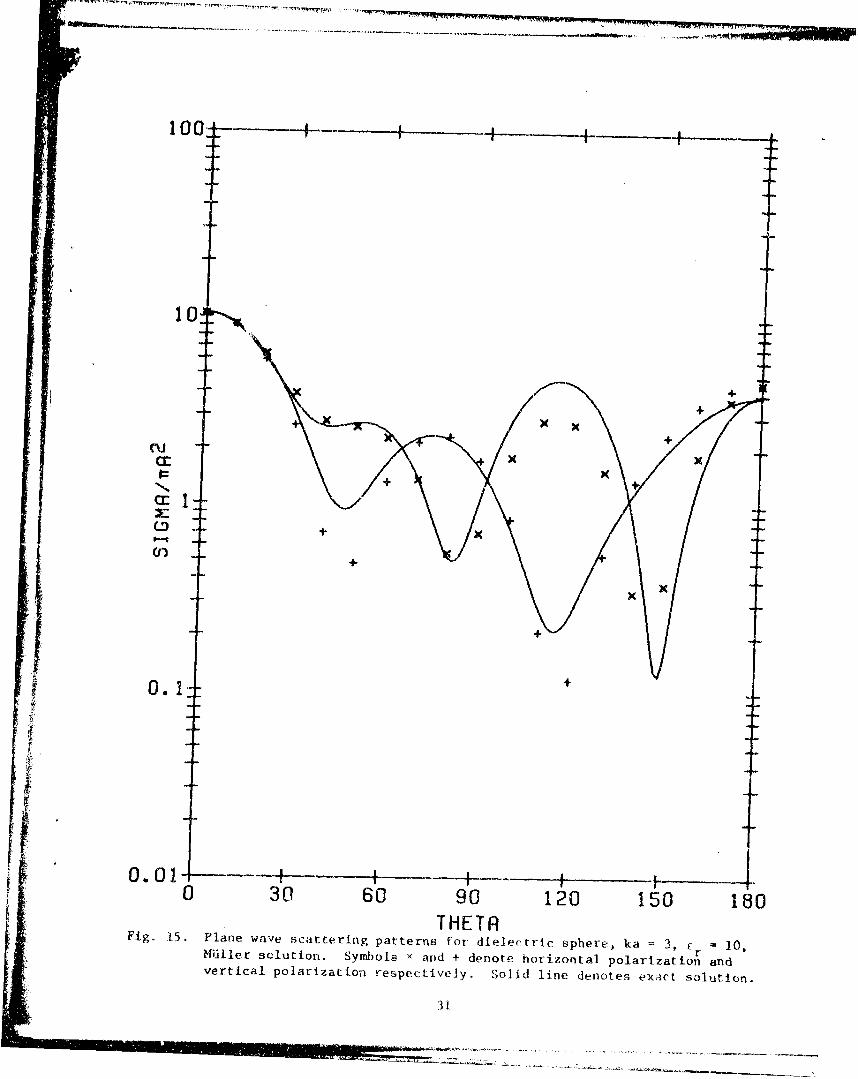
Figures 12-17 show the scattering patterns for three other dielectric

spheres. Figures 12 and 13 are for relative dielectric constant r -r ,

Figs. 14 and 15 for c: = 10., and Figs. 16 and 17 for P r-- 20. All otherr *r

[12) P. Barber and C. Yeh, "Scattering of Electromagnetic Waves by

Arbitrarily Shaped Dielectric Bodies," Applied Optc.s, vol. 14, No. 12,

I)ecenier 1975, pp. 2864-2872,

25

U ...................

0. . *m

0 0 1

0 30 o 90120 10 18

THETA ( ka- r ,-MFo iNOc'l

Figý 10 , Pj~jjc wa,.,efnsle i(..l a d v rtl ý2.Iledn wv

I10 o clot S e '(1 ,i

10:

OJ " X

C~ X

C,-)

0.1.

04,0

• 0. 30 60 90 120 ISO ISOTHETR

SFig. 11. Plane wave scat ering pat-terns fot dielectrilc sphere, ka 3, ,rMiii er solution. SymboIs - and + denote horizontal polarizat:on andiL. vertical polarit:ation respectively. SolId line denotes exaict solution.

27

0.1 ~ * + +

tC'jcc

U,

0.001 - +

!+ X

X

0.0001- LI0 30 60 90 120 150 180

THETRFig. 12.. Plane w.... s.t.ring patuLens for dielectric sphere, ka = 3, f. 1 1.1.+ r

PMCUW ýioJuto.f. Symbols x and + denote horizontal polarization andvertical polarization respectively. Solid line denotes exact solution.

- •28

L .. ............. . . ...

0. Ix

N

'z 0.01(D

Cni

0.001:_

0.0001-- ,0 30 60 90 120 150 180

THETRFig. 13. Plane wave scattering patterns for dielectric sphere, ka - 3, c r 1.1,

MUller solution. Symbols x and + denote horizontal polarization andvertical polarization respectively. Solid line denotes exact solution.

29

10 0*

10

X • X "

x

• x XC~"C

a:N+

+

0.1-

r -T

0.01 I I -+,------__0 30 60 90 120 150 180

THETAFig. 14. Plane wave scattering patterns for dielectric sphere, ka - 3, e r 10,

PMCHW solution. Symbols ý and + denote horizontal polarization andvertical polarization respectively. Solid line denotes exact solution.

30

100

10

+ +

(U +CC X X

+ X

cr1

- X

S0. Im +

0.10 1

0 30 60 90 120 I50 180THETA

Fig. 15. Plane wave .scattering patterns for dielectric sphere, ka = 3, 10 l,Miill-er solution. Symbols x and + denote horizontal polarizationr and

vertical polarization respectively. Solid line denotes exact solution.

l-7; 1- + 1 -,- - , ý , ,4 " , ý l p ý ,' , , ý, l" ." w " - . , - , .. .. -.-.- --.-.. _

100

+

x x

+ VP

+ +

Sx +

X: x

0.01

lIP

O0 O1 - - ±--~--f-4, -- j-

0 30 60 90 120 150 180THETR

Fig. 16. Plane wave scattering patterns for dielectric sphere, ka 3, r 20,PMCHIW solution. Symbols - and + denote horizontal polarization andvertical polarization respectively. Solid line denotes exact solucion.

32

10 r

+xVP+

K

cr-

LD +

U)x

+x

x KKx

0.1.

o 30 60 90 120 150 180

Fig. 17. Plane wave- sc-it tering pat terns jor cifi 1ect rc sphere, ki 3, r 20,

Miflio-r solution. Svrnhol, an + mil denote horizontal polarizat ion and

v(- rt telp'I tztio respect i vely. So1iid I *n denote eAtxac t solution.

100 •- 4 -. .. ,'

10 x +x +

x +X +

x x XWxX xx x-

+ x x+ x

x+ xcc• + x

+ x

cr1C.) + +6*--ý

+

O+

+: +

++

0.1

+ +

[9

SO0. 0 1 - -+F - ....---- ±+0 30 60 90 120 150 180

THETRFig. 18. Plate wave scattering pattern-, for fTinite dilecktric cylinder of radius a

and height. 2a. a - 0.25 fro space wavelen4ths, 4. PM(HW solution.Symbols - and f denote horizontal polarizath4m and1 vertical polarizatlionrespectively.

34

100I

x÷+x x +-X +

x +-x +

x x xxx+ x

x+ x

(\U xCC x-

+ xS+

Cc 1S+ XxxX ,D

+

+ +

++

0.01+

0.01 ! I I ,, II0 30 60 90 120 150 180

THETRFig. 19. Plane wave scattering patterns for finite dielectric cylinder of radius-a

and height 2a. a = 0.25 free space wavelengths, c = 4, MUller solution.Symbols x and + denote horizontal polarization and vertical polarizationrespectively.

35

parameters in Figs. 12-17 are the same as in Figs. 10 and 11. In Figs. 12

and 13, values less than 0.0001 are plotted at 0.0001.

Figures 18 and 19 show the computed scattering patterns of a finite

dielectric cylinder of radius a and height 2a when a is 0.25 free space

wavelengths. The relative dielectric constant of the cylinder is c = 4.r

The incident field is a plane wave traveling in the positive z direction,

the same field which was incident upon the previous dielectric spheres.a _a

Figure 18 shows -- and as obtained from our solution of the PMCHW7ra Tra

formulation. Figure 19 shows and as obtained from our solution

ira ira

of the MWller formulation. The patterns -- and 2 are plotted with theira ira

symbols x and + respectively.

The equivalent currents which radiate the patterns of Figs. 18 and 19

were obtained by using a 48 point Gaussian quadrature formula for all inte-

grations in 0. All integrations in t over the functions {f.(t)} were done byJ

sampling each f Wt) four times. The {f. (t)} consisted of 11 overlapping

triangle (divided by the cylindrical coordinate radius) functions equally

spaced in t. More precisely,

NP = 25

NPHI = 48 (73)

MT = 2

where the above variables are input data for the computer program described

and listed in Part Two, Section V.

VI. DISCUSSION

According to Figs. 12 and 13, 1he 3cattering patterns obtained from

our solution of the MUller formulation are more accurate than those ob-

tained from our solution of the PMCHW formulation for the dielectric sphere

with ka = 3 and Er = 1.1. From plots not included in this report, we ob-

served that both our PMCHW solution and our MUller solution for the equivalent

367 rI0

currents on the dielectric sphere were reasonably accurate. However, the

following argument shows that when c r is near one, a slight inaccuracy in

the equivalent currents could affect the scattering patterns drastically.

As cr approaches one, the equivalent electric and magnetic currents

approach n x Hi and Ei x n respectively whereas the scatterning patterns

approach zero. This means that the equivalent electric and magnetic

currents produce fields which nearly cancel each other. Hence, a slight

inaccuracy in the equivalent currents could cause a large percentage

inaccuracy in the scattering patterns.

We believe that our MUller solution is more accurate than our

PMCHW solution whenever cr is close to one. When a and 8 are given by

(22) and (23) as in the Miller formulation, the left-hand sides of (9)

and (10) approach -M and J respectively as c approaches one. In this.A. r

case, the expected solution

J n x H'iJAn×H-

M E X n

can be obtained by inspection of (9) and (l0). However, if a 8 = 1

as in the PMCHW formulation, the solution to (9) and (10) is not obvious

when E = 1 because the field operators on the left-hand sides of (9)r

and (10) are not diagonal. With our Killer solution, the matrix on the

left-hand side of (39) would become tridiagonal for c = 1 if its firstr

two rows of submatrices were interchanged. With our PMCHW solution, no

such simplification of this matrix is possible for c r = 1.

We recommend at least 10 expansion functions per wavelength per

component a].ong the generating curve of the dielectric body of revolution.

For example, if the generating curve were one wavelength long, the order

of the square matrix on the left-hand side of (39) should be at least 36.

The number 36 is arrived at as follows. There should be at least 9 expan-

sion functions per component of current. We say 9 expansion functions

rather than 10 because we are using overlapping triangle functions with no

peak of triangle function at either ends of the generating curve. There

are two components of electric current and two components of magnetic

current.

37

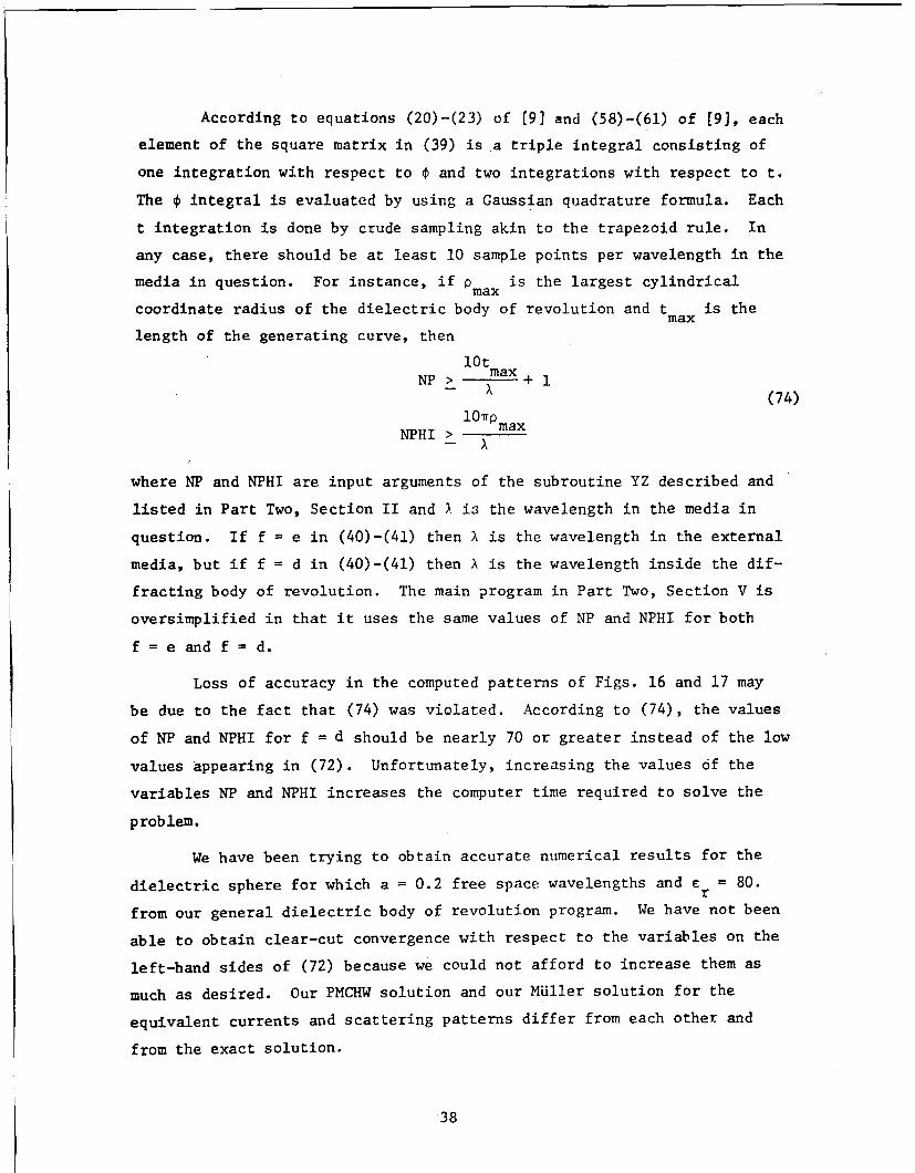
According to equations (20)-(23) of [9] and (58)-(61) of [9], each

element of the square matrix in (39) is a triple integral consisting of

one integration with respect to ý and two integrations with respect to t.

The 0 integral is evaluated by using a Gaussian quadrature formula. Each

t integration is done by crude sampling akin to the trapezoid rule. In

any case, there should be at least 10 sample points per wavelength in the

media in question. For instance, if p max is the largest cylindrical

coordinate radius of the dielectric body of revolution and t is themax

length of the generating curve, then

lotmax

NP> - +1- A(74)1 0 •Pmax

NPHI >

where NP and NPHI are input arguments of the subroutine YZ described and

listed in Part Two, Section II and A is the wavelength in the media in

question. If f = e in (40)-(41) then X is the wavelength in the external

media, but if f = d in (40)-(41) then X is the wavelength inside the dif-

fracting body of revolution. The main program in Part Two, Section V is

oversimplified in that it uses the same values of NP and NPHI for both

f = e and f = d.

Loss of accuracy in the computed patterns of Figs. 16 and 17 may

be due to the fact that (74) was violated. According to (74), the values

of NP and NPHI for f = d should be nearly 70 or greater instead of the low

values appearing in (72). Unfortunately, increasing the values of the

variables NP and NPHI increases the computer time required to solve the

problem.

We have been trying to obtain accurate numerical results for the

dielectric sphere for which a = 0.2 free space wavelengths and e = 80.r

from our general dielectric body of revolution program. We have not been

able to obtain clear-cut convergence with respect to the variables on the

left-hand sides of (72) because we could not afford to increase them as

much as desired. Our PMCHW solution and our MUller solution for the

equivalent currents and scattering patterns differ from each other and

from the exact solution.

38

For the sphere, each element of the square matrix or the left-bhad

aide of (39) can be written as a sum over the infinite set of spherical

modes. So far, we have not been able to successfully implement this alter-

nate evaluation of the matrix elements in terms of spherical modes. Th e

major diffi, ulty sebems o be lack of agreement of a few matrix elements for

which botb expansion and testing functions are near one of the poles of the

sphere.

Both the PMCIIW solution and the MUller solution are obtained by taking

a linear combination of (5) and (7) and a lipear combination of (6) and (8).

There are two other possibilities which are

(1) A linear combination of (5) and (6) and a linear romhli-

nation of (7) and (8).

(2) A linear combination of (5) and (8) aixd a linear combi-

nation of (6) and (1).

These other two possibilities give rise to alternative numerical solutions

which may compare favorably with the PMCHW solution and the MUller aolutlon.

3

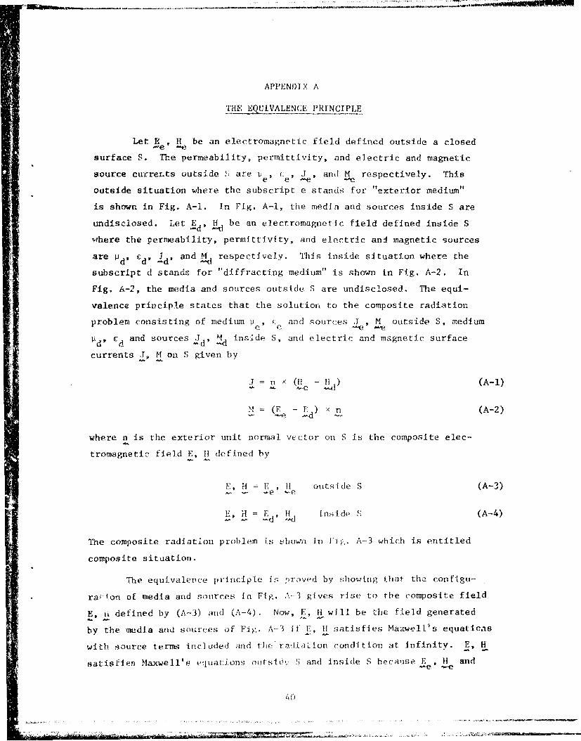
APPENDIX A

T°HF EQUIVALENCE PRINCIPLE

Let IR , if be an electromagnetic field defined outside a closed

surface S. The permeability, permittivity, and electric and magnetic

source currents outside .1 are je', C-e J , and M respectively. This

outside situation where the subscript e stands for "exterior medium"

is shown in Fig. A-1. In Fig. A-1, the media and sources inside S are

undisclosed. Let Ed, H be an electromagnetic field defined inside S

where the permeability, permittivity, and electric and magnetic sources

are pd' Cd jd' and M respectively. This inside situation where the

subscript d stands for "diffracting medium" is shown in Fig. A-2. In

Fig. A-2, the media and sources outside S are undisclosed. The equi-

valence principle states that the solution to the composite radiation

problem consisting of medium vi, ý . and sources I , M outside S, medium

d td and sources Jd' M inside S, and electric and magnetic surface

currents J, M on S given by

J = x (if -H (A-1)- (A-ei).

M = (E - E ) n (A-2)-d-e d

where n is the exterior unit nornal vector on S is the composite elec-

tromagnetic field E, if defined by

i, H 1 , U outside S (A-3)

E, H E' td inside S (A--4)

The composite radiation problem is shown in Fi g. A-3 which is entitled

composite situation.

The equivalence principle is -•vr')Vf'd by showing that the configu-

ra."%on of media and sources in Fig. A-3 gives rise to the composite field

E, ai defined by (A-3) and (A-4),, Now, E, H will be the field generated

by the media and sources of Fiý:. A-3 if E, If satisfies Maxwell's equations

with source terms included and the' radia ion condition at Infinity. E, H

satisfies Maxwell's equations outs1ic:x ; and inside S because Ee, H and

140

---= &, --

- E , .Mn

undisclosed mediaand sources S

Fig. A-1. Outside Situation.

undisclosed mediaand sources, n

l d' Ed9'T d'-d )S

Fig. A-2. Inside Situation.

E ,if -

-- ltd) (•e-Ed~d)S

,t = r il ( -H) = OS -E ) n-

' ^'- d

d~

Fig. A-3. Composite Situation.

41

E , H satisfy Maxwell's equations outside '; and inside S respectively.

E, H also satisfies the radiation condition at infinity because E , 11

satisfies the radiation condition at infinity. It remains to be shown

that Maxwell's equations for E, H exhibit the surface current sources

J and M given by (A-i) and (A-2).

It is well known that a surface current source on S gives rise to

a discontinuity across S of the tangential. component of the field. The

preceding statement is easily verified by means of an argument based on

the integral forms of Maxwell's equations. Now, this same argument can

be construed to imply that a discontinuity across S of the tangential

component of the field gives rise to a surface current source on S.

Hence Maxwell's equations for E, H exhibit the electric and magnetic

surface current sources J and M on S given by (A-1) and (A-2). There--

fore, E, H is the solution to the composite radiation problem shown in

Fig. A-3 because E, H satisfies Maxwell's equations with sources and the

radiation condition at infinity.

42

. . .

"APPENDIX B

PROOF THAT THE SOLUTION TO EQUATIONS (5)-(8)_IS UNILUE

The solution J, M to (5)-(8) will be unique if the associated set

of homogeneous equations

-n x E = 0 (B-I)

-n x H = 0 (B-2)

E+=-n ×E d 0 (B-3)

-n x 14 0 (B-4)

has only the trivial solution J = M = 0.

From (B-l) and (B-2), J, M radiate in 1i, C to produce a field

whose tangential components are zero just inside S. Hence, according

to the relation between J, M and the discontinuity of tangential field

across S as exemplified by (A-l) and (A-.2), the field Ee, H radiated by

J, M in ui c outside S satisfiese e

n2×xH = J (B-5)

E x n = M (B-6)

just outside S. See Fig. B--i.

From (B-3) and (B--4) the electric and magnetic currents -J, -M radiate

in Pd' tCd to produce a field whose tangential components are zero just outside

S. Hence, according to the relation between -J, -M and the discontinuity of

tangential field across S, the field -Ed -- d radiated by -J, -M in i'd, £d

satisfiesn - (-H• J (B-7)

(-E d n - M (B-8)

just inside S. See Fig. B-2.

The equivalence principle is used to combine the outside situation

in Fig. B-i with the inside situation in Fig. B-2 to obtain the composLte

situation shown in Fig. B-3,. Because of (B-5)-(B-8), the composite

43

Pe ' Ce

E ,H --

'eI 'e' Ce

Zero field

M

Fig. B-1. Radiation of J,M according to (B-i) and (B-2).

"Id ,cdn

U'd' C'dZero field~-

~d "-d

-Ed --14d

ig B-2. Radiation of -J, -M according to (B-3) and (B-4).

e e

Edld

Fig. B-3. Composite Situation.

44

situation in Fig. B-3 is source-free. Therefore, the field in Fig. D-3

is zero everywhere. Hence, the fields in Figs. B-I and B-2 are zero

everywhere which implies that J = M - 0.

Thus, the solution to (5)-(8) is unique because the associated set

(B-l)-(B-.4) of homogeneous equations has only the trivial solution.

45

:-;• " ~ ~ ~ ~ ~ ~ O A -. ... rý_: ., . ... . ........•_ m * • • ............... .. ..... .... .. .......... . .

APPENDIX C

MORE EXAMPLES

The equivalent currents and scattering patterns for the dielectric

spheres for which c r - 4 and ka = 4, 5, and 6 are plotted in Appendix C.

Figures C-i to C-4 are for ka = 4, Figs. C-5 to C-8 are for ka - 5, and

Figs. C.-9 to C-12 are for ka = 6. All other parameters are the same as in

Figs. 8-il in Section V. In particular, the input data for the computer

program which generated the method of moments results plotted in Figs. C-i

to C-12 is given by (72).

It is evident from Figs. 8-11 and Figs. C-1 to C-12 that the method

of moments solutions for the equivalent currents and scattering patterns

are not as accurate at ka 4, 5, and 6 as at ka = 3. Loss of accuracy

at the higher values of ka may be due to violation of (73).

46

3 S Id HJDUNd0 C) o 0 C) C 0 0 CD C0 CD D CD C00 C~j WO ýO C~ tfl C'J (\I (0 ('D C

I iO 1 10 :c

X~ 0 0

+ X + + x . j

x + 4

+0 x x

a: xc

__ __ __ __ __ _ 0 H 0 tH 0

+ x0 0 -

xx (Y)

+ x

w 4

0 0

co c~ U tiC CD CD p) I i

c nmCD) -io -m ---- ±---r u

0P4-

0)

1_ (0 + 4

+ + 1 -

bo 0

M) 0 0 C C) CD CD C) C) M) 0) C C) 000 C\J (Dc j co co Cdj co U) Nd COD

I1 0

CC) ) J-4

C) CDCd w

CD 0

UD

___4 -H

CD ---- 4 -CD

Lo Lfl :31 cm C - CD co (0 :r CM CD >

jani INnUW alflINOU

a) C

pcu

CD CD CD C) (D C C:) C) C) 0) CD CD CD CD W0

C0 (NI Lo co MN CoD Co (N o CC) (0i (j p

I IC)I C) uc1

(.)C

-r -44 w,

(IC)

cd

UD UI)C) ('Q-T C-

I0( I .I N!-H

XI

48

100:~I

* x+

10: + +

+\ x

cc+x++

cr1 x

0. 1

0 30 60 90 120 150 180THEIR

Fig. C'-3. Plane wave scat tering pattu* rim for (41tlctri ci sphert-, kit% 4, v 4, PM(:IAWsltojit on. SvmonI, , andi 4 denote o: mt pol;.iri ',at ion -ind vertic~al polarl-zat ion respvct i yelv. "SAn 1 IIioue d*uo tes I'xNr t -0 hit iufl.

4 Q~

100. I I

10:

+ +

S! 'a:j HP

�D+

C,-

0. 1

0.01 i I I I -0 30 60 90 120 150 180

THETAFig. C-4. Plane wave scattering patterns for dielectric sphere, ka = 4, c = 4,

MUller solution. Symbols x and + denote horizontal polarization and

vertical polarization respectively. Solid line denotes exact solution.

50

]9BHd0

C C) C CDCD CD CD C'J CD CD c D CD 0 CD r

co (V CDCo (J 0 D,- c 4i c

+ x

x en + CDn U

+

x Oj 110(1

Wa)

0r) 0Y

CD Cco + Lo

+

+0 >

ionflNOHW ]onflhNOHW

0p

CD 0D CD'0 CD CD CD M CD CD CD CD

-~ -D I Cn -

en +en g g+ + m-

LU (CD-~ 0 CC4.

yy cv + x-

+c X, +CC 1-I>

CDenD

COfhIO) LL)fM INUw+ +bx

+ 41

-4*

*00

F-- (A)

CD C)C ~ CJ -CD )C CD 14b0

]~~7 LUHc ]LH n (IC

-~ ~~~ ,- I '- I -

___CD ±CD

co !i M- C< CDU )D~u~ >

-D 0 --- 0 D ) r DM r.X

ý4)

~IIY-I J CO

C) !

+ x 0

tz- ~ ~ ~ ( --- ------- -- ~ Z4

too

x tx +

+ x

+ I

I + ++

x

I

0.1I +

0 30 60 90 120 150 180

HP,. C--7. P'.~ane wave sicitter-Ing patLterns- fori' I i ;pilJ ~ F=4 PMCPW

polari,; ac;,('fl resp'.ct iveiv. So I 1) exac iIn nu n

VP

C HP liHp

cr ~+X

a:

VP +

++

)+ ,

9x

l VP + -

0.

so 60 90 120 150 180THETR

Fig. C,-U Plane wave scatterhlng pattern• for dielectric sphere, ka = 5 = 4,

M~'-_•r , utl Symbol, , and +- denote hori :?ontal polar izaAion and

, 1,. lca polari:.,atl on resp(,'tivelv. Sclid line deno tes exact solution.

54

CD C) cl CD Ji CD C 3 Ci CD Uci Ci c0 N oCC) (XI (Xi (X3 Oj (.L) to CXi CC)

} + CD +7 (D 0C

,x + a4 1

+ +

CI ci+ (-0-

24-4ci~~ý

4.c -4D

--- 7--- M

ý41

ci~M Ci ci C~i Ci Ci C) CD Mi C i i

1-4 t

0 D C D 0 C CD C-)- CD M- C) 0 D

Ci I i 0r

I I+ x

+ + 1--

xX CEX CL

7CDCDUJ - +

+ ,~~CD-- +X Ci 0)

+ x+Ti-- C) :11112-C -* ) ::v----*----- -r - C-) ----- r---)- -\- C

(C) 0I F) I'I N 9H 10 fC) iX I N Ci

~ej~ ]Ufl1N~)UW ~x UHII~55

ioll-111 im d'i'l Iglo

3SHHJ ISHHJC:) C-) C:) C:) CD CD nD CD C.) CD C) CD CD C) 0

'fD (X CD (i (JO 0) (Ii WD to MX , 41

I I lC) I CD -

-'-

+ C

~~CD C) 11

+4-- 0

+ +

'4-4

0)-4O4

-CD CD

i C) CD c

Ln CDlM Ijto U)m ( CD w:'-

u >(

.-. 0)

0 w~- 4-

m dl

-* CD 0 C) C CD C- -) -- * CD 0 CD-CD CD CD Q) Cl

CC f () C\J CO (.o C] mi ((o CM 'o CD N U

i~~~~~~ In CDN~U OlIIOCC) CC)

56+

"" O

" li10:

: i

VPI

-4

VP +

(%T

0.01- + -0 30 60 90 120 150 180

THETAkFig. C-11. Plane wa'e scattering patterns for d(elect,'ic sphere, ka = 6, F_ = 4,

PMCHW solution. Symbols - and +- denot ht orizontal polarization and verti-cal polarization r-espectively. Solid iriCe denotes exact solution,

'A '57

100-

I Ox

HP

x

clucr-

cr 1:-

xx(n x •

VP

0.1 -

x +

"•i ~o. ol ,0 30 60 90 120 150 180

THETRFig. C-12. Plaiw wave scattering paI , for ditelrtc spcre, ka = 6, 4

Mliller solution, Synth0I: and 4- denote porizontal polarization and

vertical po I arizat.oo, rI-pptwcl ivelv. So" id lIne denotes exact solut ion.

..............

PART TWO

COMPUTER PROGRAM

I. INTRODUCTION

The computer program calculates the equivalent electric and magnetic

currents (58) and (59) and the scattering patterns (70) for a loss-free

homogeneous dielectric and/or magnetic material body of revolution immersed

in an axially incident plane wave. This computer program consists of a

main program and the subroutines YZ, PLANE, DECOMP and SOLVE.

Part Two consists of definitions of the input and output for the

subroutines YZ, PLANE, DECOMP, and SOLVE, listings of these subroutines,

definitions of the input and output for the main program, a verbal flow

chart of the main program, and a listing of the main program with sample

input and output. The subroutines YZ and PLANE are similar to subroutines

of the same name in [10]. The subroutines DECOMP and SOLVE are, except

for dimension statements, exactly the same as in [13]. Hence, the insides

of the subroutines YZ, PLANE, DECOMP, and SOLVE are not described in detail

in Part Two. Because these subroutines are quite complicated, a black box

approach is suggested wherein the user is concerned with just the input and

output of these subroutines. However, the user is encouraged to delve

inside the main program and to make any changes therein that he deems neces-

sary to suit his needs.

II. THE SUBROUTINE YZ

Description:

The subroutine YZ(NN, NP, N-PHI, M, MT, RH, ZH, X, A, Y, Z) stores the

matrices Ynf and Znf defined by

y tt y t•nf nf

Ynf = (75)-

nf nf

Znf = 1 0 (76'

nf nfJ

59

fIby columns in Y and Z respectively. The submatrices on the rIght-hand

sides of (75) and (76) are given by (40) and (41). The fir&t 9 argu-

ments of YZ are input variables. Except for the new input variaoles M

and MT, the subcout:`ne YZ is the same as the old subroutine YZ on pages

17-21 of [LO]. If M I- and MT = 2, Lhese subroutines are exactly the

same as far as the calculation of Y and Z in terms of the rest of the

input variables ic conceýned.

M - 1 for field evaluation just inside S and M = + 1 ior field

evaluation just outside S. M = - I if f = e in (75) and M = + 1 if

f - d in (75). The value of M is riot used in (,a.culating (76) because ,he

tangential components of the electric field operator Ef in (4].) are con-,

tinuous across S. All numeical integrations over t of fj (t> appcaling

ip (35) and (36) are donei by somrpling each f.(t) 2*A' t The v'epre-

sen*ations of pfi(t) and 1± (,,ff(t)) given b} (66) anr, (67) of [9] i'rei ~dt

replaced by representations which contain 2*MT iLnpulse functions !"steae of

4 impulse functions. For instance, (66) of [9] is replaced by

2 *MTP f t =- T 6t (77)fi~t k p + (i -1) *2 *MT (-p+ ( i-1) *MT)p-1

i-:l,2,. . .N where N wilt be defined in the paragraph which follows the next

paragraph. The T's appearing in (77) will be defined by (78).

Seven of the input variabht-s are the same as in the old subroutine

YZ on pages 17-21 of [101. These var~iables; are defined in terms of variables

appearing in [9] by

NN " i

NP P, page 9

Nt}II : N4,, page IPil~l I kpI Patge 9

411(i) kz., page 9

X(k) ->k page 13

A(k) , paA-+ 1i

6i0

In summary, n denotes the ejný dependence in (35) and (36), (pip z ),

i-l,2,.o.P are coordinates on the generating curve, the k which multi-

plies p1 and z i the propagation constant, and xk and Ak are the

abscissas and welghts for the N point Gaussian quadrature integration

in 0. Note that NP-i shoilld be an integer multiple of MT. If NP-i is

not an integer multiple of MT, the program will ignore PH(i) and ZH(m)

for

[(NP -l)/MT]*MT+l < m < NP

where [(NP-I)/MT] is the largest integer which does not exceed (NP-1)/MT.

Minim-am allocations are given by

COMPLEX Y(4*N*N), Z(4*N*N)

DIMENSION RH(NP), ZR(NP), X(NP1I), A(NPHI), D(NG)

PD(NG), TP(2*MT*N), CR(NPHI), Cl(NPHI), C2(NPHI),

C3(NFHI), C4(NPHI)

COMMON RS(NG), ZS(NG), SV(NG), CV(NG), T(2*MT*N)

whe re

N =- [(NP-i1)/MTI - 1,

NG - (N+1)*MT

The variable,4 in comnnon make the results of some intermediate calculations

done in YZ available to the subroutine PLANE described irn Sertion TII of

Part Two.

We mention a few portion:' of YZ which differ Yrom tho subroutine

listed on pages 18--21 of [10]. Equatl.on (29) of [9] has been generalized to

2 1T 2*MT*(J-!t)+1 d11 j 2 C. +q 2 d

'k k d + ý d(79)AT2,MT,_M ! A, - M +q 2 T MT *.+ I

for J 1,2,,,.N and 1 1,2,....MT where

MY

. * (-i(80)

A, k d%1 I' -1).MT.....

el

and the d's are given by equation (28) of [9]. Note that A1 is the

electrical length of generating curve over which the first half of

f (t) exists and that A2 is the electrical length of generating curve

over which the second half of f (t) exists. The generalization of

equation (68) of [9] is

2*M*(JkdM,,(j)+i82)

T' -kdMT*J+I (83)2*MT*J-lMT+ A2

for J = 1,2,...N, and I = 1,2,...MT where A1 and A2 are given by (80)

and (81). Expressions (78) - (83) are calculated in DO loop 68. DO

loop 12 accumulates A in DEL. DO loop 1.9 puts (78) in T(2*MT*(J-I)+I)

and (82) in TP(2*MT*(J-I)+I). DO loop 15 accumulates A2 in DEL. DO

loop 16 puts (79) in T(2*MT*J-MT+I) and (83) in TP(2*MT*J-MT+I).

The subscripts KT, LT, and il Inside DO loop 32 are obtained as

follows. Since the generating curve consists of NG = (N+I)*MT small

intervals, it is composed of (N+I) large intervals where the mth large

interval consists of the ((m-l)*MT+l)th through the (m*MT)th small

intervals. The index I of DO loop 60 denotes the Ith small interval.

The Ith small interval is contained in the (19+l)th large interval where

19 - (I-1)/MT]. The second half of f 1 9 (t) and the first half of f 9+1(t)

are in this large interval. The index K of DO loop 32 denotes f l9+K-(t).

Since T((m-l)*2*MT+I) thr,.•ign r(m*2*MT) is allotted to f (t), ra=l,2,.... .I,

f (t) is preceded by (m-1) overlaps. For each overlap the subscript of Tm

increases by an amount MT not accounted foi" by f. Hence, replacing m by

19+K-1, we arrive at, the subscript

KT -I + (19+K-2)*MT

for T. Here, KT is the field subscript which refers to the testing

functior. By analog), the source subscrlpt LT whichl refers tc the expan--

siorn function Is given by

I1T J + (J9+I,--2)*KT

62

Retaining flg+Kl(t) as the testing function, we take the analogously

subscripted function f (t) to be the expansion function and arriveJ9+L-l

at the matrix subscript

Jil = (J9+L-2)*N2 + 19+K-1

where, as in the program, N2 = 2*N,

ttDO loop 17 ac•umulates in R1 the contribution to (Y n) of

n J,Jequation (31.) of [9' due to the term in equation (32) of [9].

iThis cuntribution is given by

2 *MTR1 = T +2,MT(JI)* T * PD(I+MT*(J-1))I i+2M*T~) I+. *MT* (J-l)

where, as in the program,

PD(i) =- M * -

Here, the factor -M not included tn eciation (32) of [9] provides for

the choice of field evaluatior efther outside or inside S.

ttDO loop 18 accumulates in .J I le contiibution to (Y n J-,J

equation (31) of [9] due to Oie 7-- term in equat.ion (32) of [9].d.p.I11

This contribution is given by

R1 ''I+2*MT*(1.--L)-MT 'I+2*N*,'*(J.-1)riA!

LISTING UF THE SUbROUTINE YZ

SUBROUTINE YZ(NN,NP, r,"HI ,M,MT,RHZHX,AY,Z)COMPLEX UY (784),Z(784),G1,G2,G3,G4,G5,G6,YI,y?,Y3,Y4,ZI,Z2,Z3,Z4DIMENSION Pt, lII6i),ZH(161),XC48hAI48),D(160 ,Pl( 160),TP(320)0IMENSION Ck(48),CI(4•9),C2(48),C3(48) ,C4(48)COMMON RS(160),ZS(160i,SV(160) ,CV(I6O) ,T(320)PI=3.1415931

Pl M=-M*PIN= (NP-i) /MT-1N2=2*NNG= ( N+ 1 )*MTNGM= NG3-MTMT2= MT*2DC 57 I=i,NG &

12= 1+1

DZ=Z H( 12 )-ZH ( I )0(1 =SQRT( DR*DR+DZ*DZ)

RS (1)=.5*( RH( 12)+RH( I ))

SV(I )=DR/D( ICV( I )=DZ/D( I)PD( I )=PIM/C(D1 )*RS(I 1

* 57 CONTINUE~j1=0J 5=0DO 68 J=1.NDEL=0-DO 12 1=1,Ml*J1=J1+1DEL= DEL+DH JI)

12 CONTINUEJL=J 1-MTSN=0.00 .19 1=.1 MT,15=J 5+ 1J1=J 1+1SN=SN~D( ji)TP (J!--) =0(J 1)/DFLT(J5h'(SN--.5*D(JM)*TP(J5)

19 C01k4e INUFDEL= 0.00 15 L=1,MTj1= I I-&flFL=.FL+D(J].I

15 CO1NTIIN UFJ1I J 1--MT

j I = j 1 + ISrK=SN-D(J1 I

I( Jd (. ) N -- r't( 1: 1 ) 1 "T PCj16 tt'NT iNtiF

dl zJl,-MT

Pi t) 2 f f 1.r N H

(""-- 1* ~ ý Pif

9'( P (K)(

(~~~~~' 1 .)F1SI~ ) N WC 'HIN)

C 4(K )25 CONTINUE

N2N=N2*NN4N=N2N*2DO 62 J=i,N4NY( J) =0.Z(J)=0.

62 CONTINUEU=(0.91.)D00 59 J=1,NGFJ=FN/RS(J)

L2=2IF(J.LE.MT) L1=2IF(J.GT.NGM! L2=1

JT=J+MT*(J9-2)J5=( J9-2)*N2-1s1=l.DO 60 I-1tJi9=(I-1)/MT

J6=19+J5FI=FN/RS( I)RP=FKS(J)-RS(I)ZP=ZS( J)-ZS ( I)R2=RP*RP+ZP*ZPIF(I.NE.J)) GO TO 41Si=. 5P<2=. 0625*D(J)*D(J)

41 R3xTRS( I)*RS (J)GL=0-G2=0 -

G3=0..G4=0.G5-O.

Onf 61 Kzrl.NPHIP'4=R2+R3*CR (K)R5=SQPT(R4)Zjh S)/fk5*(CCS(FR5)-U,*Sl N( R5))Y1=z i*( 1.tU*R5)/R4GIC 1t (K) *YI +GlG2=C2(KJ*Y1 -G2G3--C3M K)*'Y1+G3G4=C 4 iK) Z I +G4G'5= C ?(K ? 16, I G 5

61 CCJN71NUE

y C ( V(j )-z~p*SV(i i) (I ) CV!J)*Gl'Y2=(RS(.J)*SV( 1)*CV(,i -R, 11)*SV(;*CV( [-zP*IV( I *SV(J) l*G3Y 3=Z V* 6 3Y4=(PP*CVgI)--2P*SV(1))i*G2+RS(J)*CV(t)*GI

G 1.- U*G47?=- SV( J )(

G2=- FP*G'

23=zSVC I )*GG3 =F J*L64 65

Z4=U*( G5--F I*G; )

K2=2

DO 31 L=Llt12Ll=J'T+MT*Lj7=J6+ L*N2DO 32 K=K1,K2KT=I T+MT*KTT=T(LT' IT(KT)Jl=J7+KJ2=J 1+NJ3=j 1+N2NJ4=J 3+NY(JI )=TT*Y1+Y( Jl)Y(J2)::TT*Y2+Y(J2)YiJ3)=T'F,.-Y3+Y(J3)Y(j4)=TT*Y4+V( J4)

Z(J.)=TT*ZI+TP(LT)*TP(KT)*GL+Z(JiIZ(J2)=TT*Z2+TP(LT)*T(KT)*G2+Z1J2)Z(J3)=TT**Z3*TP(KT)*T(LT)*G34-ZU3I)Z(J4)='TT*L4-#Z(J4)

32 CONTINUE31 CONTINUE60 CONTINUE59 CONTINUE

N2P= .N2+ 1KD1=1J10oJ5=0DO1 11 J=1,NR1=O.DO 17 I=1.MT2-

J5=J5+1Rl=k1+T(Jfl*T( JlI P' (ji

17 CONYINUE,il=J L-MT2J5=j 5-MT2K02=KDI+NKD3=KDI +N2NK04=KO3+NG1=Y (K~l )-Y(K[)4)Y(KD1)=1il+(;lY( KD2)=O.Y tKD3 )=OY( KD4) =f<1-G1Z(KDl)=Z(KDl)+Z(KDl)Z(KD2) =7 (KD2 )-Z( K03,1Z(K[P?)-Z(KD2)Z(KD4)=ZBKU(4)4Z(KD4)IF(J-1) 26,27,26)

27 Jl=-JI+MT2J5 = i ') M IGO 10l ?2

26 KU1=KDI-1KU2 =KP?-- 1K U 3=K 3-1

66

KU4z.4(D4-11KoI - N2

KL2=KD2--N2K L3 =K()3 --N2KL 4= KD 4- N 2

00 18 I-19MT

J1=J1+1J 5=J 5+ 1RlP, 1+1(11) *T( Jl-MT) *FD(J5)

18 CONTINUEJ1=J 1+MTGl=Y (KUl )-Y( KL4)G2=Y (KU4)-Y(KL I)Y(KU1) =P1+Gl,Y(KU2) =Y(KU2)-Y(KL2)

Y(KU)3)=:Y(KU31-Y( KL3)Y(KtJ4)=RI+G2Y (KLI)=PRL-G2Y(KL2) =-Y(KL2)Y(KL3) =-Y(KU3)Y(KL4)=P.1-GIZ(KU1)=Z(KUI )#Z(KL,)Z(KU2) =Z(KU21-Z(KL3)Z( KU3) =-Z (KU3 )-Z( KL2 )

Z(KU4) =Z (KU4) +Z(KL4)Z(KL I1) =Z (KUl)Z( KL 2) =-Z( K1J3)Z(KL3) =-Z( KU2)

Z(KL4) =Z(KU4)22 KDI=KDI+N2P11 CONTINUE

I&F(N.LT.'3) RETURNJ2=N2DO 13 I=3tNJ2=j 24N2J1=1 -2Ktl =1DO 14 J=11JL,(.IJ.1J2+JKLJ2.zKU3.+NKU 3=KU I +N2N'K LJ4= KUI3 + NKL2=:KL 1+NKL3-IKL 1+N2rN4KL4z KL.3+NY (KL, )A=-Y (KU4)

Y( K[.2)=-Y( KU2)Y(KL3) ý>-Y(KL3)Y( KL 10 =-Y( KUl

Z (KL 2) =-Z ( KU 3)Z(Kl.3)=-Z(KU2)L(KL 4 ) =/(KU4)

14 CCNTINUEF

PETU PýE NO

III. THE SUBROUTINE PLANE

Desc riptiýn:

T7he subroutine PLANE(NN, N, MT, NT, THR, R) puts R of (49) innj

R(J + (w-l)*N+(L-1)*4*N) where J=1,2,...N, m=l denotes pq = te, m-2

denotes pq . ¢9, m=3 denotes pq = tý, m=4 d~notes pq = , and L=l,2,...NT.

Here, L denotes the Lth value of the receiver angle 0 . The first 5r

arguments of PLANE are input variables. Except for the new input vwitable

MT, the subroutine PLANE is the same as the old subroutine PLANE on pages

22-26 of [10]. If MT = 2, these subroutines axe exactly the same as far

as the calculation of R in terms of the rest of the input variables is

concerned.

The integration of f.(t) over t inherent in (49) is approximated

by sampding fj(tW 2*MT times instead of 4 times. The representation of

t, f(t) given by (66) of [9] is replaced by (77). NN is the value of n

appearing in R2pq. It is required that NN > 0 but this requirement causes

no real loss of generality because Rq is either even or odd in n, N isn]

the number of expansion functions lying on the generating curve. Specifi-

cally, N is the maximum value of i in (77). THR(L) is the Tth value of

the receiver angle 0 where L = 1,2,...NT. The variables RS, ZS, SV, CV,r

and T appearing in the conmnon statement e.rly in the subroutine PLANE are

input variables calculated by calling the subroutine YZ beforehaad. The

calculated values of these vatiables depend only on the seecond, fifth,

sixth, and seventh arguments (NP, MT, R11, Z1) of YZ,

Minimum allocations are given by

COMILEX R(4*NT*N)

DIMENSION TIIR(NT), BJ(M)

COMMON RS(NCG), ZS(NG), SV(NC), CV(NG), T(2*MT*N)

where

NG = (N+] l*M•

and M is the largest of the values of M calculated by PLANE. The sug-

gested allocation B.f(Q0) will work if the maximum circumference of the

body of revolution is less than 26 wavelengthis.

68

Most of the statements In the subroutine PLANE are the same as

or very similar to statements in the old subroutine PIANE listed on

pages 25-26 of [10]. The major difference is in the calculation of

the subscript (TT+MT*K) for T and the subscript 1l for R, Using

reasoning similar to that used to obtain the subscripts KT and J1 in the

subroutine YZ, we arrive at

(IT + MT*K) = I + (19 + K-?)*MT

J1 = 19 + K-I

where19 = [(I-l)/MTr]

The above Jl is valid only for L=I. If L 1 1, then (L-I)*4*N must

ae added to this l.

LISTING OF THE SUBROUTINE PLANE

SUJBROU1 INF OLANE(NN, N, MT,NT,THR,R)

COMPLEX R11064),U,UI ,U2,R1,R2,R33R4

DIMENSION THR(37),BJ(5 0 )

COMMON RS(160),ZS(l60)),SV(160),CV(160),T( 3 20)

NG=( N+I •*MTU=(0., I.)Wl=3 .141593*LU'*NNN4=4*NJ P, - N,4 ' NT

D( 2? J=l,,JV.

22 CCNT I N UFJ5=- IDO 129cs1 8 R I i

SN 2 -0. I¢'{T•,

PIFA C I =,NG

IHI,'..LF..5F: 7• (,;J TO IY

MC2. xi÷ 13.- 2r /x

IF(M .L, F. ( tN+ ;') ) GO IA[ 19

18 BJIzO.

B J 3 0.

I C (] . FO .0 %Ž' •

,J t = •i- 1

DO 14 .J=39MJM= J M-i1.F3j(jM) =jm/X*Bj(JI4-I)-8J(JM+2)

14 CONTINUES~o.DO 15 J;-.3pM9,'S=S+BJ (J)

1.5 CONTINUEs=BJ(Q1)+2.**S13J2= BJ (NN+ I) /S8,13= J (NN-2 )/BJI=-BJ3IF(NN.GT.0) BJ1=EIJ(NN)/S

24 ARG=ZS(1)*CSU2=UI*(CCS(ARG)+U*SIN( AR0)R4= BJ 3-BJ 1 ) U*U2R2=( BJ3+BJI)*u2R1=-BJ2*CV( I)--cSN*U2+CS*SV(I)*R4R3=SV( I)*R2R2=-CS*P219=1 1-1)/MTI T= I .MT* (19-2)J7=19-.J5K22l

IF(J9.EQ.N) K2=1DO 20 ~K1,lK2TThl(1 T +MT *K),;1 =.J 1+ KJ2=1 14NJ3=.J 2+NJ4=J 3-ANR(JI )=TT*R1+R(Jl)R~(12 )-rTT*R2tR(J2)R(J3 )-VT*P3+R(J3)R(J4 )=Tr*P,44-R( J4)

20 CONTINJUE13 CGNTINUE

J5=J5+N412 CCNTINLJF

RE I iiRNEN D

70

IV. THE SUBROUTINES DECOMP AND SOLVE

Description:

The subroutines DECOMP(N,IPS,UL) and SOLVE(N,IPS,UL,B,X) solve

a system of N linear equations in N unknowns. These subroutines will

be used in Section V to solve the matrix equation (39). The input to

DECOMP consists of N and the N by N matrix of coefficients on the left-

hand side of the matrix equation stored by columns in UL. The output

from DEiOpu is IPS and UL. This output is fed into SOLVE. The rest of

the input to SOLVE consists of N and the column of coefficients on the

right-hand side of the matrix equation stored in B. SOLVE puts the' solution to the matrix equation in X.

Minimum allocations are given by

COMPLEX UL(N*N)

DIMENSION SCL(N), IPS(N)

in DECOMP and by

COMPLEX UL(N*N), B(N), X(N)

DIMENSION IPS(N)

in SOLVE.

More detail concerning DECOMP and SOLVE is on pages 46-49 of [13]

LISTING OF THE SUBROUTINES DECOMP AND SOLVE

SIBROUTI NE DECOMP( Nt IPSUL)CMPLFX LJL (3136) PIVOTEMDIMENSION SC L( 6),IPS( 56)DO 5 Iz-1,NIPS(I)=IRN=O.J1=1DO 2 J=1,NULM=ABS(REAL(Ui..(jl)) )'+AB,'(AIMAG{UlL(Jl))

Jl=J I+NIF(RN--ULM) 1,2,2

I R4--ULM2 CONT INLJE

SCa ( I1=1./RN5 CONTINUE

NM1=N-i; .,.K2-0

DO 17 K=I,NMI

DO I1I I K 9NIP= IPS(JiIPK= IP+K2

71

SIZE=(ABS(REAL(UL(IPK)))+ABS(AIMAG(ULIIPK)))l*SCL.(IP)I-(SIZE-BIG) 11,1140I

10 BIG=.sIZEIPv= I

11 CONTINUE

14 J=IP S( K)IPS(IK)=IPS( IPV)IPS( 1PV)=J

15 KPP=IP-S(K)+K2PIVOT=UtL(KPP)KPIr:K+ 1DO 16 1=KP19NKP=KPP1Pz=IPS( I )+K2EM=-UL (IP) /PIVOT

18 UL(IP)=-EMDO 16 J=KI~NIP=I P+NKP=K P+NUL( I P)--4JLl IP)+EM*UL( 1(P)

16 C ONT INU EK 2 2 +N

17 CONT INUEREYU RNENDSUBROUTINE SO!LVE(NIPS,ULBX)COMPLEX ULM336),oB(56)#X(56)vSUMlDIMENSIONJ IPS(56)NPi=N+ I!P=!PS-( 11X( 1) =B(IP)DO 2 I=2,NIP=I PS( I)IPB= IIIIM1l 1-lstUmý 0.Dc I J-zlIMi.SUJM: SIJM-4UM- I IP)* WJ)

I I PzzlP4N2 X ( I ) F IPB -SU M

I P=-I PS ON) +K 2XI N) =X ( N) /IJL. I P)of)~ a lBA(k,=2¶N

S UM 0.I P=z IpIý00 3 ,J=11[11,NIrzhI P+

3 SdM= SUM)V Ut.. I P *X (J4 X ( Al)=( X ( I[ S UM)/UL I PI

P FT P l

72

V. THE MAIN PROGRAM

Description:

The main program calculates the electric and magnetic currents

(58)-(59) and the normalized scattering cross sections=- and (70)

for the e polarized axially incident (6t = 180') plane wave (50)-(51).

The main program calls the subroutines YZ, PLANE, DECOMP, and SOLVE.

The main program is short and simple. It is a representative applica-

tion of the theory in Part One of this report.

Input data is read early in the main program according to

READ(I,10) NP, NPHI, MT, NT

10 FORMAT (413)

READ(l,Il) BK, UR, ER, ALP, BET

11 FORMAT(MEl4.7)

READ(l,12)(RH(I), 1=1, NP)

READ(l,12)(ZH(I), 1=1, NP)

12 FORMAT(IOF8.4)

READ(l,II)(X(K), K=l, NPHI)

READ(l,11)(A(K), K=l, NPHI)

The input variables NP, NPHI, MT, RH, ZH, X, and A are very

similar to variables of the same names in the argument list of the sub-

routine YZ. In summary, (RH(i), ZH(i)), i=l,2,...NP, are the cylindrical

coordinates (P.i z.) on the generating curve, 2*MT is the number of values

of t at which f (t) is sampled for the purpose of numerical integration,

and X and A are respectively the abscissas and weights for the NPHI point

Gaussian quadrature integration in 4.

The scattering cross sections are evaluated at receiver angles

O = (J-l)7r/(NT-l) radians for J=I,2,...NT. BK is the propagation* r

constant k in the external medium. This k appears in (50)-(51). UR

and ER are respectively the relative permeability and the relative

C e

permittivity C- of the body of revolution. Here, p d and cd are the

epermeability and permittivity of the (diffracting) body of revolution

73

and ve and e are those of the external medium. ALP and BET are respec-tively the constants a and 8 appearing in (39). The PMCHW solution is

obtained by setting a = 8 = 1. The MUller solution is obtained if a and

8 are given by (22) and (23).

Minimum allocations are given by

COMPLEX YE(4*N*N), ZE(4*N*N), R(4*NT*N),

B(4*N), YD(4*N*N), ZD(4*N*N), Y(16*N*N),

C(4*N)

DIMENSION RH(NP), ZH(NP), X(NPHI), A(NPHI),

THR(NT), RC(N), IPS(4*N)

whereN = [(NP-1)/MT] - 1

Statement 38 puts Yle defined in accordance with (75) by

[ tt Yt,]

=le . (84)

~le leJ

in YE and Zle defined in accordance with (76) by

lee

lel "I

le= (85)

in ZE. Storage of Yle and Zle is by columns.

Statement 39 puts the matrix R defined by

r te 0t

11

R, = I (86)

in R. The column vectors on the right-hand side of (86) appear in (56).

For receiver angle 6 = THR(J), RI of (86) is stored by columns inr

R((J-1)*4*N+l) through R((J*4*N).

74

DO loop 22 uses (56) to store the right-hand side of (39) in B.

DO loop 22 also puts 2 /(kp1*MT+lI) in RC where pIMT+I is the cylindrical

coordinate radius evaluated at the peak of the triangle function inherent

in fl (t).

Statement 40 puts Yld defined by

d tt Yld

ld ld

Yld 1 (87)

Lld ld I

in YD and Zld defined by

z tt ztýld ld

Zld = (88)

~d Zid

in ZD. Storage of YId and Zld is by columns.

Nested DO loops 26 and 27 put the first two columns of submatrices

on the left-hand side of (39) in Y. The index J of DO loop 26 denotes

the Jth column of the composite square matrix on the left-hand side of

(39).

Nested DO loops 28 and 29 put the third and fourth columns of sub-

matrices on the left-hand side of (39) in Y. The index J of DO loop 28

denotes the (2*N+J)th column of the composite square matrix on the left-

hand side of (39).

Statements 41 and 42 solve the matrix equation (39) for the com-

posite column vector consisting of V 1 1 i, and II. This composite

column vector is stored in C.

At the peak of the Jth triangle function, the n=l term of the

equivalent electric current (58) reduces to

75

1 0 . (2/p tI u Cos0+ (2j/pj+l) i J sin (89)

DO loop 31 prints the real and imaginary parts of

teUl = (2/(kPMT*J+l))II

the real and imaginary parts of

U2 = (2j/(kPMTJ+l))I8

and the magnitudes of Ul and U2. Here, Ul is the t component of the

equivalent electric current in the E plane and U2 is the 0 component

of the equivalent electric current in the H plane when the y component

of the incident magnetic field is minus one at the origin.

At the peak of the Jth triangle function, the n=l term of the

equivalent magnetic current (59) reduces to

1 M8 = ( 2 j )V to (2/pn * + -e ucos * (90)P *J+llJ -t MT*J+I lJI

DO loop 34 prints the real and imaginary parts of

B(J) = (2j/(kp•,J+I)) t

and the real and imaginary parts of

U2 = (2/(kpM T,))Vlj

and the magnitudes of B(J) and U2. Here, B(J) is the t component of

the equivalent magnetic current in the H plane and U2 is the 0 component

of the equivalent magnetic current in the E plane when the x component

of the incident electric field is minus one at the origin.

Nested DO loops 35 and 36 calculate and print -and of (70).

Inner DO loop 36 accumulates the portion

/

76

Rt kvtO + Rll + tIt+ 011

of (62) in ET and the portion

-kt6R 0te -teo + -to.te + 00-1R 1, + R, 11 -i

of (63) in EP. The W1 and W2 printed in DO loop 35 are respectively

and for receiver angle e= (Jrl)*ir/(NT-l) radians.A'- r

Suggested modifications of the main program are:

1) Changing the normalization of the scattering patterns.

For example, one could replace (70) by (69). All scat-

tering patterns in Part One, Section V are plots of (69).

*2) Removing the restriction that the values of the input

arguments NP, NPHI, MT, RH, ZH, X, and A of the subroutine

YZ be the same in call statements 38 and 40. This modifi-

cation is indicated by (74).

3) Generalizing from axial plane wave incidence to oblique

plane wave incidence.

The above three modifications can be realized without tampering with

any of the subroutines YZ, PLANE, DECOMP, and SOLVE.

The sample input and output accompanying the listing of the

main program is for the dielectric sphere with ka = 1 and c r = 4.

77

LISTING OF THE MAIN PROGRAM

//P3M JOB (xxXX,XXXX,1,2),'MAUTZ,JOE',PEGION=200K// EXEC WATFIV//G3.SYSIN DD$JOB MAUTZ,TIME1l, PAGES=40C SUBRCUTINES YZ, PLANE, DECOMP, AND SOLVE APE CALLED.

COMPLEX YE(784) ,ZE(784b.R(1064) ,B(56),YD(784),Zf(784),Y(3136)COMPLEX Cl56)vU,U1,U2,FT,EPvCONJGDIMENSION RH(161),ZH(161),X(48),A(48),THR(37)hRC(19) ,IPS(56)READ(lv1O) NP,NPHIMT,NT

10 FORMAT(413)READQ1, 11) BK,9UR,E R,AL P,BET

11 FORM AT f5E14.7)READ(1,12) (RHII) ,I=1,NP)R EAD (1I912) (ZHI 1),11,~lNP)

12 FORMAT(10F8.4)READ (119 11) ( X( K) , K= 1, NPHIREADI 1, 11)(A(K) ,K= 1qNPHI)WRITEI3,13) NP,NPHIMTNT

13 FORMAT(' NP NPHI MT NT'/IIX,13,15,213))WRITE(3 ,14) BKqURERALP,BET

14 FORMAT(7X,IBK*,12X,IURS,12XOER',11X,IALPI,11X,IBETI/(lX,5E14.7))WPITEI3, 15)(RH(I),I=1, NP)

15 FORMAT(' RH'I/(1Xtl0F8.4) )

16 FORMAT(I' ZH I/( 1X,10OF 8.4) )W~RITEl3 ,17) (X(K) ,K=1 ,NPHI)

17 FORMAT(' X'/IlX,5El4.7))WR IT El3, 18) 1Al K) ,K=1,NPHI)

18 FORMAT(* At/IIX,5E14.7))DO 119 J=l,NPRH(J )=BK*RH(J.)ZH( J)=BK*ZH (J)

19 CONTINUE38 CALL YZI1,NP,NPHI ,-1,MT,RHZHX,A,YEZE)

WR ITE13 ,20) (YEll), 1 1,4),(ZEII), 1=1,4)20 FORMAT(' SOME ELEMENTS OF YE AND ZEl/(1X,4E14.7))

P1=3.141593DT=Pl/hiNT-1)DO 21 J=lvNTTHF (J)= (J- 1)*DT

21 CONTINUEN=(N P- 1) /MT- 1

39 CALL PLANE(I1N,MT,NT,THRR)N2=2*NN3=3*NN4=4*NNTN=(NT-1)*N4DO 22 I=1,NJ3=I+N'TNBlI)=R(J3)BI I+N)=-P(J3+N)B(I N2)=-R(J3+N3)BI I+N3)=-RIJ3+N2)RC(II)=2./RH(MT*I+1)

22 CONT IN UEWRITF(3,23)(E;l I),11,9N2)

23 FORMAT($' HALF OF THE ELEMENTS OF Ei'IIIX,4E-14.7))FM=SQRT I UR*ER)

78

DO 24 1=1,NPtiPI )=EM*RH( I)ZH( I )=EM*Z H( I)

24 CONTINUE40 CALL YZ(1,NP,NPHlI , MTRHtZH,X,A,VD,ZD)

WRITE(3,25)(YD(IhI1=1,4),(ZDI) ,1=1,4)25 FORMAT(f SOME ELEMENTS OF YD AND ZD'/(IX,4E14.7VJ

D=SQRT(UR/ER)ALPD=ALP*DBETD=BET/DJY= 0J1=ODO 26 J=1,N2DO 27 I=1,NJY=JY+1J1=J.1+1J2=J 1+NY(JY )=YE( J2 )+ALP*YD(J2)Y(JY+FN) =-YE (JI )-ALP*YD WJ 1)Y(JY+N2 )=ZE (J2)+BETD*ZD( J2)Y(JY+N3)=-ZE( J1)-BETD*ZD(J1)

27 CONTINUEJY=JYg-N3jl=j 1+N

26 CONTINUEJ1=ODO 28 J=19N2DO 29 1=10N2JY=JY+ 1j 1=J 1+ 1YCJY)=ZE(Jl)+ALPD*ZD(J 1)Y(JY+N2)=YE (Ji )+BET*YD(J1)

29 CONTINUEJY=JY+N2

28 CONTINUF41 CALL DECOMP(N4,IPStY)42 CALL SOJLVE(N4,IPS,Y,BC)

WRITE( 3, 30)30 FORMAT('Q REAL JT IMAG JT REAL JP IMAG JP MAG JT

IMAG JP')U=(0.9 1.)DO 31 J=1,NRk=RC(J)ET=U*RP,B(J) -=ET*C(J)

UI-1{=P'C (J4N2

tl;)=FT*(C(J+N3)hi=CAE3S( 01l)W2=CABS( U2)IPITE(3,32) UlU2,WI,W2

32 Fc1RMAT(lX,6E11.4)31 CONTINUE

WP+ITE( 3,3"3)33 FOR.MAT('0 REAL MT IMAG? MT REAL MP IMAG MP MAG MT

iMAG MPI)DO 34 J=1,N

wl=CABS(B(J)) 79

W2=CABS(U2?)WRITEf3,32) B(J],U2,WItW2

34 CONTINUEWRIT E(3,37)

37 FORMAT('O SIGTHETA SIGPHI')CON= .25/P1**3JR1=0DO 35 J=1,NTET=O.EP=O.DO 36 I=1,N2JC2= I+N2JR1=JR1+1JR2=JR1+N2ET=ET+R(JR2 )*C(I)RR(JR1)*C(JC2)EP=EP-R(JRI )*C( I)+R(JR2)*C(JC2)

36 CONTINUEJR1=JR1+N2WI=C ON*ET*CONJG( ET)W2=C CN*EP*CCNJG( EP)WRITE(3,32) WIW2

35 CONTINUESTOPEND

$ OAT A21 20 2 190.1000000E+01 0.1000000E+01 0.4000000E+01 0.IO00000E+01 0.1000000E+01

0.0000 0.1564 0.3090 0.4540 0.5878 0.7071 0.8090 0.8910 0.9511 0.98771.0000 C.9877 0.9511 0.8910 0.8090 0.7071 0.5878 0.4540 0.3090 0.15640.0000

-1.0000 -0.9877 -0.9511 -0.8910 -0.8090 -0.7071 -0.5878 -0.4540 -0.3090 -0.15640.0000 0.1564 0.3090 0.4540 0.5878 0.7071 0.8090 0.8910 0.q511 0.98771. 0000

-0.9931286E+00-0.963S719E+00-0.9122344E+00-0.8391170E+00-0.7463319E+00-0.6360537E+00--0.5108670E+00-0.3737061E+00-0.2277859EI 00-0.7652652E-01

0.7652652E-01 0.2277859E+00 0.3737061E+00 0.5108670E+CO 0.6360537E+000.7463319E+00 0.8391170E+00 0.9122344E÷00 0.9639719E+00 0.9931286E+000.1761401E-01 0.4060143E-01 0.6267205E-01 0.8327674E-01 0.10193C1E+000.1181945E+00 0.1316886E+00 0.1420961E+00 0.1491730E+00 0.1527534E+000.1527534E+00 0.1491730E+00 0.1420961F+00 0.1316886E+00 0.U181945E+000.1019301E+00 0.8327674E-01 0.6267205E-01 0.4060143E-01 0.1761401E-01

$STDP

//

PRINTED CUTPUTNP NPHI MT NT21 20 2 1S

BK UR ER ALP BET0.1000000E+01 0.1000000E+01 0.4000000E+01 0.1000000E+01 0.1000000E+01

RH0.0000 0.1564 0.3090 0.4540 0.5878 0.7071 0.8090 0.8910 0.9511 0.98771.0000 0.9877 0.9511 0.8910 0.8090 0.7071 0.5878 0.4540 0.3090 0.15640. 0000

ZH-1.0000 -0.9877 -0.9511 -C. 8910 -0.8090 -0.7071 -0.587'8 -0.4540 -0.3090 -0.1564

0.0000 0.1564 0.3090 0.4540 0.5878 0.7071 0.8090 0.8910 0.9511 0.9877

1. 0000x-0.9931286E+00-0.9639719E+00-0.9122344E+00-0.8391170E+00-0.746331 g I÷+00

80

-0.6 360537E+0O-O.510867OE+00-0.3737061E.OO-0.2277859E.Oo-0.7652652E-oj.0.7652652F-01 0.2277859E+00 0.3737061E+00 0.5108670E4-00 0.4360537Ee-000.7463319E+00 0.8391170E+00 0.9122344E+00 0.9639719E+00 0.9,931286F+00

A0.1761401E-01 0.4060143E-01 0.6267208E-01 0.8327675E-Cl 0.10193C1E+000.1181945F+00 0. 1316886E.CO0 .1420961E+00 0.1491730E+00 0.1527534F+000.1527534F+00 0.1491730E+00 0.1420961E+00 0.1316886E+00 0.1181945E+000.1019301E+00 0.8327675E-01 0.6267208E-01 0.4060143E-01 0.17614C1E-O1

SOME ELEMENTS OF YE AND ZE0.2431891E+01-O.5483869E--02 0.5072693E+00-0.1154096E-010.1I015252E+0O-0.2041826E-01 0.9178627F-01-0.3066700E-O10.9008127E-0l-0.7025097E+01 0.7607359E-01 0.1940044E+010.5597932E-01 0.7892063E+00 0.3345479E-01 0.2816698E+00

HALF OF THE ELEMENTS OF B-0.5464500E+oO-o.75o3574E+00-o.5449371F+oO-o. 5690688E+0O-0.4 709502E+0O-0.3229641E+00-0.2808148E+00-0.1054077E4-OO

O.0000000E+00-0. 1778790E-01 0.2808146E+00-0. 1054077E+0O0.4 7C,9504E+00-0.3229641 E+O0 0.5449370E+0O-0. 5690686E+O0O.5464502E.OO-0.7503576E+00 O.7951685E+00-0.5814634E'OO0.7044444E+0O-0.6853659E+00 0.5376098E+0O-O. 8194968E+OO0.293ý9058E+OO-0.9327149E+00-0.OOOOOOOF+O0-0.9769601Eý+OO

-0.2 939057E+O0-O .9327147E+00-o.5376099E+oo-0. 81 94970E+ 00-0.7044442E+00-0.6853657E+O0-0.7951688E+00-Q.5814636E400SOME ELEMENTS OF YD AND ZO-O.2290969E+01-0.3768066E-01-0.3189305E+00-0.7057631E-O10.9599513E-O1-O.10884T.7E+00 0.4942125E--01-0.1374637F+O00.3428959F+0O-O.2902117E+01 0.2818084E+00 0.1262741E+Cl0.2082631E+00 0.5027283E+00 0.1465860E+00 0.1911734E+oo

REAL J7 IMAG JT REAL JP IMAG JP MAG J7 MAG JP-0.6398E+O0-O.1395E.01 0.6170E+00 0.1415E+01 0.1535E+01 0.1543E+Cl-0.8349E+00-0.1227E.01 0.8652E4-00 0.1174E+01 0.1484E+01 0.1459E+01-O.1025E+01-0.9274E+00 0.7285E+00 0.9655E+00 0.1382E+01 O.1210E+Ci-0.1127E+01-0.4861E+03 0.6632E+00 0.6917E+00 0.1228E+01 0.,9582E+00-0.1094E+01 0.5150E-C1 0.4185E+00 0.6316E4-00 0.1096E+01 0.7576E+00-0.8731E+00 0.5874E+00 0.1349E4-00 0.7185E+00 0.1052E+01 0.7311E+00-0.5410OE+00 0. 1026E+01 0.1116E+00 0.1011IE+01 0. 1160E+01 0. 1017E+01-0.1626E+00 O.1320E+01-0.9319E-0OI OW.1256E+01 0.1330E+01 0.1260E+Cl0.1722E+00 0.1479E+01 0.2244E+00 0.1496E+01 0.1489E+01 0.1513E+01

REAL MT IMAG MT REAL MP IMAG MP MAG MT MAG MP-0.1 064E+00-0.68C6E+0O-0.8434E-01-0.6963E+00 0.6889E+00 0.7014E+00-0.2323E+O00-0. 5834E+00-0.2176E+O0-0.5837E+0O 0.6279E+00 0.6230E+CO-O.3712E.00-O. 4190E+00-0.1639E+0O-0. 5138E+00 0.5598E+00 O.5393E.CO-0.4731E+00-0.1809E+CO-0.1442E+0O-0.4209E+OO 0.5065E+00 O.4449E+C0-0.5072E+00 0.1093E+00-0.4617E-01-0.4199E+00 0.5188E+00 0.4224E+00-0.4451E+00 0.3992E+00 0.5351E-0I1-0.4940E+0O 0.5979E+00 0.4969E-+00-0.3171E+00 0.63q97E+00 0.7018E-01-0.6418E4-00 0.7140E+00 0.6457E+CO-0.1556E+00 0.8002E4-00 0.1272E+00-0.7901E+00 0.8152E+00 0.8003E+00-0.1304E-01 0.8852E+CO-0.1307E-01-0.8971E+00 0.8853E+00 0.8972E*00

SIGTHETA SIGPHI0.1 535E+00 0.1535E+00C.1488E+00 0.1523E+000.1355E+00 0.1489E+000.1153E+00 0.1433E+CO0.9112E-01 0.1360E+000.6592E-01 0.1272E+000.4260E-01 0.1176E+C00.2343E-01 0.1074E+CO

81

0.9801E-02 O.0722E-01O.2164E-02 0.8741E-010.1589E-03 O.7831E-010.2810E-02 O.7015E-010.8790E-02 0.6308E-010.1666E-01 O.5717E-01C.2504E-01 0.5241E-Cl0.3278E-01 0.4879E-010.3895E-01 0.4625E-010.4290E-01 0.4475E-010.4426E-01 0.4426E-01

82

RE 7E PENCES

[1] A. J. Poggio and E. K. Miller, "Integral Equation Solutions ofThre; !imensional Scattering Problems," Chap, 4 of Computer

Tec11~Ms for Electr n~oetics, edited by R. Mittra, PergamonPress, 1973, Equation (4.17).

[2] Yu Chang and R. F. Harrington, "A Surface Formulation for

21Characteristic Modes of Material Bodies," Report TR-74--7,Department of Electrical and Computer Engineering, Syracuse

University, Syracuse, NY, October 1974.

[3] T. K. Wu, "Electromagnetic Scattering from Arbitrarily-ShapedLossy Dielectric Bodies," Ph.D. Dissertation, University ofMississippi, 1976.

[4] C. MUller, Foundations of the Mathematical Theory of

Electromagnetic Waves, Springer-Verlag, 1969, p. 301, Equa-

tions (40)-(41). (There are some sign error-s in these

equations.)

[5] V. V. Solodukhov and E. N. Vasil'ev, "Diffraction of a PlaneElectromagnetic Wave by a Dielectric Cylinder of ArbitraryCross Section," Soviet Physics - Technical Physics, vol. 15,

No. 1, July 1970, pp. 32--36.

[6] N. Morita, "Analysis of Scatter~ng by a Dielectric Rectangular

Cylinder by Means of Integral Equation Formulation," Electronics

and Communications in Japan, vol. 57-B, No. 10, October 1974,pp. 72-80.

[7] E. N. Vasir'ev and L. B. Materikeva, "Excitation of Dielectric

Bodies of Revolution," Soviet Physics - Technical Physics,

vol. 10, No. 10, April 1966, pp. 140.1-1406.

[8] R. F. lHarrington, Field Computation by Moment Methods,Macmillan (Co., New York, 1968.

[91 J. R. Mant z and R. F. Harr lgt on, "IF-Field, F,'-Ftield, and

Comb nud F1eld Soltitions f(or Bod ii, of tfRevol ut ion ," Interirm

'Techl•oi 's Report RA1K;-TR- 77-109, PAIW me Ai UT' D, V;. 1] cpMtert Centter,

Cr1ff sKu; Air Force Base, Ne+w York, tFarch 1,977.

LOI 1. 8. Mautz and R. F. lParrlngton. ".ompliter frou'ram, for 11-- eld

.- F-l eld, ai:d ('o 'n14 ted 5 r i.el.d 0 olutio iim for B :od ies of ;¼'\: I tIOn

Interim Technlical Report IQAI)Q--R-- 77,-,,21.1 t one Aii Iht'veliopir<'ntCtýn ter, (;rifIis. A.Ir Force Raso,, New Nork"( 1977.

[li .t , F. 11s:<rrisr,.'tsr 'l'Sme-A[ ~r'mo•v1 c E',ctromngnu:' x n-'.Felhs,,•-Hi 1 1 i-,ýk ... . 19• gt I.. S. :\ [ 'u t ,t"6

81

[121 P. Barber and C. Yeh, "Scattering of Electromagnetic Waves byArbitrarily Shaped Dielectric Bodies," Applied Optics, vol. 14,Nio. 12, December 1975, pp. 2864-2872.

[13] J. R. Mautz and K. F. Harrington, "Transmission from a RectangularVlaveguide into Half Space 11Trough a Rectangular Aperture," InterimTechnical Report RADC-TR-76-264, Rome Air Development Center, GriffissAir Force Base, New York, August 1B76.

4

484