jose apesteguia miguel a. ballesterapesteguia/measure_rationality_welfare.pdf · a measure of...

A Measure of Rationality and Welfare

Jose Apesteguia

Catalan Institute for Research and Advanced Studies, Universitat Pompeu Fabra,and Barcelona Graduate School of Economics

Miguel A. Ballester

Universitat Autonoma de Barcelona and Barcelona Graduate School of Economics

Evidence showing that individual behavior often deviates from theclassical principle of preference maximization has raised at least twoimportant questions: ð1Þ How serious are the deviations? ð2Þ What isthe best way to analyze choice behavior in order to extract informationfor the purpose of welfare analysis? This paper addresses these ques-tions by proposing a new way to identify the preference relation that isclosest, in terms of welfare loss, to the revealed choice.

I. Introduction

The standardmodel of individual behavior is based on themaximizationprinciple, whereby the individual chooses the alternative that maximizesa preference over the menu of available alternatives. This has two keyadvantages. The first is that it provides a simple, versatile, and powerful

We thank Larbi Alaoui, Jorge Alcalde-Unzu, Stephane Bonhomme, Guillermo Caruana,Christopher Chambers, Tugce Cuhadaroglu, Eddie Dekel, Jerry Green, Philipp Kircher,Paola Manzini, Marco Mariotti, Paul Milgrom, Mauro Papi, John K.-H. Quah, Collin Ray-mond, Larry Samuelson, Karl Schlag, Jesse Shapiro, and three referees for very helpfulcomments and Florens Odendahl for outstanding research assistance. Financial supportby the Spanish Commission of Science ðECO2014-53051, ECO2014-56154, ECO2012-34202,ECO2011-25295, ECO2010-09555-E, ECO2008-04756-Grupo Consolidado CÞ and FEDER isgratefully acknowledged. Data are provided as supplementary material online.

Electronically published October 30, 2015[ Journal of Political Economy, 2015, vol. 123, no. 6]© 2015 by The University of Chicago. All rights reserved. 0022-3808/2015/12306-0002$10.00

1278

account of individual behavior. The second is that it suggests the max-imized preference as a tool for individual welfare analysis.Research in recent years, however, has produced increasing amounts

of evidence documenting deviations from the standard model of indi-vidual behavior.1 The violation in some instances of the maximizationprinciple raises at least two important questions: ð1ÞHow serious are thedeviations from the classical theory? ð2Þ What is the best way to analyzeindividual choice behavior in order to extract information for the pur-pose of welfare analysis?The successful answering of question 1 would enable us to evaluate

how accurately the classical theory of choice describes individual be-havior. This would shift the focus from whether or not individuals violatethe maximization principle to how closely their behavior approachesthis benchmark. Addressing question 2, meanwhile, should help us todistinguish alternatives that are good for the individual from those thatare bad, even when the individual’s behavior is not fully consistent withthe maximization principle. This, of course, is useful for performing wel-fare analysis.Although these two questions are intimately related, the literature has

treated them separately. This paper provides the first joint approach tomeasuring rationality and welfare. Relying on standard revealed pref-erence data, we propose the swaps index, which measures the welfare lossof the inconsistent choices with respect to the preference relation thatcomes closest to the revealed choices, the swaps preference. The swapsindex evaluates the inconsistency of an observation with respect to apreference relation in terms of the number of alternatives in the menuthat rank above the chosen one. That is, it counts the number of alter-natives that must be swapped with the chosen alternative in order forthe preference relation to rationalize the individual’s choices. Then, theswaps index considers the preference relation that minimizes the totalnumber of swaps in all the observations, weighted by their relative oc-currence in the data.To the best of our knowledge, the literature on rationality indices

starts with the Afriat ð1973Þ proposal for a consumer setting, which is tomeasure the amount of adjustment required in each budget constraint

1 Some phenomena that have attracted a great deal of empirical and theoretical at-tention and that prove difficult, if not impossible, to accommodate within the classicaltheory of choice are framing effects, menu effects, dependence on reference points, cyclicchoice patterns, choice overload effects, etc. For experimental papers, see May ð1954Þ,Thaler ð1980Þ, Tversky and Kahneman ð1981Þ, and Iyengar and Lepper ð2000Þ. Sometheoretical papers reacting to this evidence are Kalai, Rubinstein, and Spiegler ð2002Þ,Bossert and Sprumont ð2003Þ, Masatlioglu and Ok ð2005, 2014Þ, Manzini and Mariottið2007, 2012Þ, Xu and Zhou ð2007Þ, Salant and Rubinstein ð2008Þ, Green and Hojmanð2009Þ, Masatlioglu, Nakajima, and Ozbay ð2012Þ, and Ok, Ortoleva, and Riella ð2012Þ.

measure of rationality and welfare 1279

to avoid any violation of the maximization principle. Varian ð1990Þ ex-tends the Afriat proposal to contemplate a vector of wealth adjustments,with different adjustments in the different observations.2 An alterna-tive proposal by Houtman and Maks ð1985Þ is to compute the maximalsubset of the data that is consistent with the maximization principle.3

Yet a third approach, put forward by Swofford and Whitney ð1987Þ andFamulari ð1995Þ, entails counting the number of violations of a consis-tency property detected in the data. Echenique, Lee, and Shum ð2011Þmake use of the monetary structure of budget sets to suggest a version ofthis notion, themoney pump index, which considers the total wealth lostin all revealed cycles. The swaps index contributes to the measurementof rationality in a singular fashion by evaluating inconsistent behaviordirectly in terms of welfare loss. It is also the first axiomatically basedmeasure to appear in the literature. In Section III.A, we illustrate thecontrast between the swaps index treatment of rationality measurementand these alternative proposals.There is a growing number of papers analyzing individual welfare

when the individual’s behavior is inconsistent. Bernheim and Rangelð2009Þ add to the standard choice data the notion of ancillary condi-tions, which are assumed to be observable and potentially to affect in-dividual choice but are irrelevant in terms of the welfare associated withthe chosen alternative. Bernheim and Rangel suggest a welfare prefer-ence relation that ranks an alternative as welfare superior to anotheronly if the latter is never chosen when the former is available.4 Theproposal of Green and Hojman ð2009Þ is to identify a list of conflictingselves, aggregate them to induce the revealed choices, and then performindividual welfare analysis using the aggregation rule. Nishimura ð2014Þbuilds a transitive welfare ranking on the basis of a nontransitive pref-erence relation.5 The swaps index uses the revealed choices, as in theclassical approach, to suggest a novel welfare ranking, the swaps pref-erence, interpreted as the best approximation to the choices of the in-dividual and complemented with a measure of its accuracy: the incon-

2 Halevy, Persitz, and Zrill ð2012Þ extend the approach of Afriat and Varian by com-plementing Varian’s inconsistency index with an index measuring the misspecificationwith a set of utility functions.

3 Dean and Martin ð2012Þ suggest an extension that weights the binary comparisons ofthe alternatives by their monetary values. Choi et al. ð2014Þ apply the measures of Afriatand Houtman and Maks to provide valuable information on the relationship between ra-tionality and various demographics.

4 Chambers and Hayashi ð2012Þ extend Bernheim and Rangel’s model to probabilisticsettings.

5 Other approaches include Masatlioglu et al. ð2012Þ, Rubinstein and Salant ð2012Þ, andBaldiga and Green ð2013Þ. There are also papers describing methods for ranking objectssuch as teams or journals, based on a given tournament matrix describing the paired re-sults of the objects ðsee Rubinstein 1980; Palacios-Huerta and Volij 2004Þ.

1280 journal of political economy

sistency value. In Section III.B, we illustrate by way of examples otherdifferences between our proposal and these other approaches.In Section IV, we study the capacity of the swaps index to recover

the true preference relation from collections of observations that, for avariety of reasons, may contain mistakes and hence potentially revealinconsistent choices. We show that this is in fact the case for a wide arrayof stochastic choice models.In Section V, we propose seven desirable properties of any inconsis-

tency index relying only on endogenous information arising from thechoice data and show that they characterize the swaps index. Then, inSection VI, we characterize several generalizations of the swaps index,together with versions of the classical Varian and Houtman-Maks indiceswithin our framework. Section VII applies the swaps index to the ex-perimental data of Harbaugh, Krause, and Berry ð2001Þ.In the online appendix we discuss the relaxation of three assumptions

made in the setup. We first show that it is immediate to make the swapsindex capable of considering classes of preference relations with furtherstructure, such as those admitting an expected utility representation. Wethen show how to extend the swaps index to include the treatment ofindifferences. Third, we argue that it is possible to construct a naturalversion of the swaps index ready for application in settings with infinitesets of alternatives.

II. Framework and Definition of the Swaps Index

Let X be a finite set of k alternatives. Denote by O the set of all possiblepairs ðA, aÞ, where A ⊆ X and a ∈ A. We refer to such pairs as observations.Individual behavior is summarized by the relative number of times eachobservation ðA, aÞ occurs in the data. Then, a collection of observations fassigns to each observation ðA, aÞ a positive real value denoted by f ðA, aÞ,with oðA;aÞf ðA; aÞ5 1, interpreted as the relative frequency with whichthe individual confronts menu A and chooses alternative a. We denoteby F the set of all possible collections of observations. The collection fallows us to entertain different observations with different frequencies.This is natural in empirical applications, where exogenous variations re-quire the decision maker to confront the menus of alternatives in un-even proportions.Another key feature of our framework is preference relations. A pref-

erence relation P is a strict linear order on X, that is, an asymmetric,transitive, and connected binary relation. Denote by P the set of allpossible linear orders onX. The collection f is rationalizable if every singleobservation present in the data can be explained by the maximizationof the same preference relation. Denote by mðP, AÞ the maximal elementin A according to P. Then, formally, we say that f is rationalizable if there


exists a preference relation P such that f ðA, aÞ > 0 implies mðP, AÞ 5 a.6

Let R be the set of rationalizable collections of observations that assignthe same relative frequency to each possible menu of alternatives A ⊆ X.Notice that every collection r ∈ R is rationalized by a unique preferencerelation, which we denote by P r.7 Clearly, not every collection is ratio-nalizable. An inconsistency index is a mapping I : F → R1 that measureshow inconsistent, or how far removed from rationalizability, a collectionof observations is.We are now in a position to formally introduce our approach. Con-

sider a given preference relation P and an observation ðA, aÞ that is in-consistent with the maximization of P. This implies that there are anumber of alternatives in A that, despite being preferred to the chosenalternative a according to P, are nevertheless ignored by the individual.We can therefore entertain that the inconsistency of observation ðA, aÞwith respect to P entails consideration of the number of alternativesin A that rank higher than the chosen one, namely, jfx ∈ A : xPagj. Theseare the alternatives that must be swapped with the chosen one in orderto make the choice of a consistent with the maximization of P. If everysingle observation is weighted by its relative occurrence in the data, theinconsistency of f with respect to P can be measured by oðA;aÞ f ðA; aÞj fx ∈ A : xPag j. The swaps index IS adopts this criterion and finds thepreference relations PS that minimize the weighted sum of swaps. Werefer to PS as the swaps preference relations. Formally,

ISð f Þ5 minP o

ðA;aÞf ðA; aÞ j fx ∈ A : xPag j;

PSð f Þ ∈ argminP o

ðA;aÞf ðA; aÞ j fx ∈ A : xPag j :

In summary, the swaps index enables the joint treatment of incon-sistency and welfare analysis. It discriminates between different degreesof inconsistency in the various choices, relying exclusively on the infor-mation contained in the choice data, and additively considers every sin-gle inconsistent observation weighted by its relative occurrence in thedata. It identifies the preference relations closest to the revealed data,the swaps preferences, measuring their inconsistency in terms of theassociated welfare loss. In Appendix B we show that almost all collectionsof observations have a unique swaps preference; that is, the measure of

6 Notice that, since P is a linear order, if there exist a, b ∈ A with a ≠ b such that f ðA, aÞ > 0and f ðA, bÞ > 0, then f is not rationalizable.

7 The purpose here is to create a bijection between P and a subset of the rationalizablecollections. The set R is one way of creating this bijection, which comes without loss ofgenerality.


all collections with a nonunique swaps preference is zero. We then typ-ically talk about the swaps preference without further considerations un-less the distinction is relevant.8 We now illustrate the swaps index andthe swaps preference by way of two examples.Example 1. Consider the set of alternatives X 5 f1, . . . , kg. Suppose

that the collection f contains observations involving all the subsets ofX and is completely consistent with the preference relation P, rank-ing the alternatives as 1P2P � � � Pk. Now consider the collection of ob-servations g involving the consistent evidence f with a high frequencyð1 2 aÞ and the extra observation ðX , xÞ, x > 1, with a low frequency a.That is, g 5 ð1 2 aÞf 1 a1ðX,xÞ, where 1ðX,xÞ denotes the collection with allthe mass centered on the observation ðX, xÞ. Clearly, the collection g isnot rationalizable. In order to determine the swaps index and the swapspreference for g, notice that for any P 0 ≠ P there is at least one pair ofalternatives, z and y, with y < z and zP

0y. Hence, the weighted sum of swaps

for P 0 is at least ð12 aÞf ðfy, zg, yÞ. Meanwhile, preference P requires x2 1swaps in the observation ðX, xÞ, and hence the weighted sum of swapsfor P is exactly aðx 2 1Þ. For small values of a, it is clearly the case thataðx2 1Þ < ð12 aÞf ðfy, zg, yÞ, and therefore, ISðgÞ5 aðx2 1Þ and PSðgÞ5 P.Hence, in such cases the swaps preference coincides with the rationalpreference P, and the inconsistency attributed to g by the swaps indexis the mass of the inconsistent observation a weighted by the numberof swaps required to rationalize the inconsistent observation.Example 2. Let

f ðfx; yg; xÞ5 f ðfy; zg; yÞ5 12 2a2

and

f ðfx; y; zg; yÞ5 f ðfx; zg; zÞ5 a;

where a is small. That is, there is large evidence that x is better than yand that y is better than z and some small evidence that y is better thanx and z and that z is better than x. Notice that any preference in whichy is ranked above x or z is ranked above y has a weighted sum of swapsof at least ð1 2 2aÞ/2. There is only one more preference to be ana-lyzed, namely, xPyPz. This preference requires exactly one swap in menufx, y, zg, where y is chosen, and also one swap in menu fx, zg where z ischosen. The weighted sum of swaps of P is therefore 2a, which, forsmall values of a, is smaller than ð1 2 2aÞ/2, and hence ISð f Þ 5 2a and

8 In addition, in App. C, we deal with the computational complexity of obtaining PS.


PSð f Þ 5 P. That is, the swaps preference rationalizes the large evidenceof data,

f ðfx; yg; xÞ5 f ðfy; zg; yÞ5 12 2a2

;

and incurs some relatively small errors in f ðfx, y, zg, yÞ 5 f ðfx, zg, zÞ 5 a.

III. Comparison to Alternative Measures

A. The Measurement of Rationality

In a consumer setting, Afriat ð1973Þ suggests measuring the degree ofrelative wealth adjustment that, when applied to all budget constraints,avoids all violations of themaximization principle. The idea is that, whena portion of wealth is considered, all budget sets shrink, thus eliminat-ing some revealed information, and thereby possibly removing some in-consistencies from the data. Thus, Afriat’s proposal associates the degreeof inconsistency in a collection of observations with the minimal wealthadjustment needed to make all the data consistent with the maximiza-tion principle.We now formally define Afriat’s index for our setting. Let wA

x ∈ ð0; 1� bethe minimum proportion of income in budget set A that must be re-moved in order to make x unaffordable. Then, given a menu A, if aproportion w of income is removed, all alternatives x ∈ A with wA

x ≤ wbecome unaffordable. We say that a collection f is w -rationalizable ifthere exists a preference relation P such that f ðA, aÞ > 0 implies that aPxfor every x ∈ A /fag with wA

x> w. Notice that when w 5 0, this is but the

standard definition of rationalizability. Afriat’s inconsistency measure isdefined as the minimum value w * such that f is w*-rationalizable. Notethat we can alternatively represent this index in terms of preferencerelations, making its representation closer in spirit to that of the swapsindex. To see this, suppose that P * is a preference that w*-rationalizes f.Then, for all observations ðA, aÞ with f ðA, aÞ > 0, all alternatives xP *amust be unaffordable at w *. Hence

w* 5 maxðA;aÞ:f ðA;aÞ>0

maxx∈A;xP*a

wAx :

Since no other preference can w -rationalize f for w < w *, it is clearly thecase that we can define Afriat’s index as9

9 For notational convenience, let maxx∈∅ wAx 5 0.


IAð f Þ5 minP

maxðA;aÞ:f ðA;aÞ>0

maxx∈A;xPa

w Ax :

Varian ð1990Þ considers vectors of wealth adjustments w, with poten-tially different adjustments in the various observations. Then, Varian’s in-dex identifies the closest vector w to 0 that, under a certain norm, w-rationalizes the data. Here, given the structure of the swaps index, weconsider the 1-norm and define Varian’s index as follows:

IV ð f Þ5 minP o

ðA;aÞf ðA; aÞ max

x∈A;xPawA

x :

Houtman andMaks ð1985Þ propose considering the minimal subset ofobservations that needs to be removed from the data in order to makethe remainder rationalizable. The size of the minimal subset to be dis-carded suggests itself as a measure of inconsistency. It follows immedi-ately that, in our setting, the Houtman-Maks index, which we denote byIHM, is but a special case of Varian’s index when wA

x 5 1 for every A andevery x ∈ A.Finally, rationality has also been measured by counting the number of

times in the data a consistency property is violated ðsee, e.g., Swoffordand Whitney 1987; Famulari 1995Þ. Consider for instance the case of theweak axiom of revealed preference ðWARPÞ. In our context, WARP isviolated whenever there are two menus A and B and two distinct ele-ments a and b in A \ B such that f ðA, aÞ > 0 and f ðB, bÞ > 0. Hence, we canmeasure the mass of violations of WARP by means of

IW 5 oðA;aÞ;ðB;bÞ:fa;bg⊆A\B;a ≠ b

f ðA; aÞ f ðB; bÞ:

Recently, Echenique et al. ð2011Þmade use of the monetary structure ofbudget sets to suggest a new measure, the money pump index, whichevaluates not only the number of times the generalized axiom of re-vealed preference ðGARPÞ is violated but also the severity of each vio-lation. Their proposal is to weight every cycle in the data by the amountof money that could be extracted from the consumer. They then con-sider the total wealth lost in all the revealed cycles. To illustrate thestructure of this index in our framework, let us contemplate only vio-lations of WARP ði.e., cycles of length 2Þ. Consider a violation of WARPinvolving observations ðA, aÞ and ðB, bÞ. The money pump reasoningevaluates the wealth lost in this cycle by adding up the minimal wealth~wAb that must be removed to make b unaffordable in A and the minimal

wealth ~wBa that must be removed to make a unaffordable in B.10 Then,

10 Notice that ~wAx , assumed to be strictly positive, is measured in dollars while Afriat’s and

Varian’s weights wAx are proportions of wealth.


~wAb 1 ~wB

a represents the money that could be pumped by an arbitragerfrom the WARP violation. Now, given the vector of weights ~w, the WARPmoney pump index can be defined as11

IW2MP 5 oðA;aÞ;ðB;bÞ:fa;bg⊆A\B;a ≠ b

f ðA; aÞf ðB; bÞð~wAb 1 ~wB

a Þ:

In order to illustrate the differences between all these indices and theswaps index, let us reconsider example 1. Consider then two differentscenarios in which x5 k and x5 2, that is, gk 5 ð12 aÞf1 a1ðX,kÞ and g2 5ð1 2 aÞf 1 a1ðX,2Þ. Intuitively, collection gk involves a more severe in-consistency, since the observation in question is one in which the indi-vidual chooses the worst possible alternative, alternative k, while ignor-ing all the rest. Collection g2 also shows some inconsistency with themaximization principle, but this inconsistency is orders of magnitudelower, since it involves choosing the second-best available option, that is,option 2. It follows immediately from the discussion in example 1 thatthe swaps index ranks these two collections in accordance with the aboveintuition, that is, ISðgkÞ5 aðk 2 1Þ > a5 ISðg2Þ. Afriat’s and Varian’s judg-ment of these collections depends crucially on themonetary values of thealternatives, which need not necessarily coincide with the welfare rankingand hence may lead to counterintuitive conclusions. For example, if 1 isthe least expensive alternative in menu X, that is, wX

1 ≥ wXt for all t ≤ k,

Varian’s approach involves removing income until alternative 1 becomesunaffordable, regardless of the scenario. Hence, both collections wouldbe equally inconsistent. Note that, for Afriat, the mass of violations isirrelevant, and hence if removing option 1 from X is costly and removingalternative k from all menus is cheaper, it may be the case that gk is w -rationalizable for some value w < wX

1 , while g2 is not. Therefore, Afriat’sindex may judge gk as being less inconsistent than g2. With respect toHoutman-Maks’s index, since the inconsistencies in both scenarios are ofidentical size, a, IHM does not discriminate between them. Finally, theassessment provided by WARP violation index IW depends on the specificnature of f. To illustrate, consider, for example, that k 5 3 and that

f ðX ; 1Þ5 f ðf1; 3g; 1Þ5 f ðf2; 3g; 2Þ5 b

and

f ðf1; 2g; 1Þ5 12 3b:

It follows immediately that

11 It is immediate to extend this index to consider cycles of any length, something thatwe avoid here for notational convenience.


IW ðgkÞ5 3abð12 aÞ < ð12 aÞað12 2bÞ5 IW ðg2Þ

whenever b < 1/5, and hence scenario 2 is regarded as the more in-consistent of the two. Although index IW2MP weights both sides of theabove inequality by ~w, the inequality still holds for certain nonnegligiblevalues of b.

B. The Measurement of Welfare

Let us illustrate our approach to welfare analysis by contrasting it firstwith two proposals: Bernheim and Rangel ð2009Þ and Green and Hoj-man ð2009Þ. Although these two papers tackle the problem from dif-ferent angles, they independently suggest the same notion of welfare.Let us denote by P the Bernheim-Rangel-Green-Hojman welfare rela-tion, defined as xPy if and only if there is no observation ðA, yÞ with x ∈ Asuch that f ðA, yÞ > 0. In other words, x is ranked above y in the welfarerankingP if y is never chosen when x is available. Bernheim and Rangelshow that, whenever every menu A in X is present in the data, P is acyclicand hence consistent with the maximization principle.We now examine the relationship betweenP and the swaps preference

PS. It turns out to be the case that the two welfare relations are funda-mentally different. It follows immediately that PS is not contained in Pbecause PS is a linear order, whileP is incomplete in general. In the otherdirection, and more importantly, note that while P evaluates the rank-ing of two alternatives x and y by taking into account only those menusof alternatives in which both x and y are available, PS takes all the datainto consideration. Hence, PS andP may rank two alternatives in oppo-site ways.Nishimura ð2014Þ has recently proposed a different approach, the tran-

sitive core. Given a complete nonnecessarily transitive relation ≽, thetransitive core declares an alternative x preferred to alternative y when-ever, for every z, ðiÞ y ≽ z implies x ≽ z and ðiiÞ z ≽ x implies z ≽ y. LikeP ,the transitive core may be incomplete, and since relative frequenciesare not considered, the transitive core may go in the opposite directionto PS.We illustrate the differences between the swaps preference and the

proposals here presented, using example 2 above. We argued there thatxPSyPSz. Note now that zPx since x is never chosen in the presence of z,and hence P and PS follow different directions. Moreover, if ≽ is un-derstood to be the revealed preference, y is ranked above x by thetransitive core, and hence this is different from PS too.Finally, notice that the swaps preference PS comes, by construction,

with the associated inconsistency IS, which provides a measure of thecredibility of PS. A low value of IS naturally gives credit to PS, while high


values of IS may call for more cautious conclusions regarding the truewelfare of the individual, either by focusing on subsets of alternativesover which violations are less dramatic ðin the spirit of the aforemen-tioned approachesÞ or by adopting a particular boundedly rationalmodelof choice.

IV. Recoverability of Preferences and the Swaps Index

Consider a decision maker who evaluates alternatives according to thepreference relation P but when it comes to selecting the preferred op-tion sometimes chooses a suboptimal alternative. Mistakes can occur forvarious reasons, such as lack of attention, errors of calculation, misun-derstanding of the choice situation, trembling hand when about to se-lect the desired alternative, inability to implement the desired choice,and so forth. Whatever the specific model, mistakes generate a poten-tially inconsistent collection of observations f. This raises the issue ofwhether the swaps index has the capacity to recover the preference re-lation P from the observed choices f.We show below that the swaps index identifies the true underlying

preference for models that generate collections of observations in which,for any pair of alternatives, the better one is revealed preferred to theworse one more often than the reverse. Formally, we say that the collec-tion f generated by a model satisfies P-monotonicity if xPy implies thatoA⊇fx;ygf ðA; xÞ ≥oA⊇fx;ygf ðA; yÞ, where the inequality is strict wheneveroa∈fx;ygf ðfx; yg; aÞ > 0. In order to assess the generality of this result, wefirst show that a diverse number of highly influential classes of stochasticchoice models satisfy this property.Random utility models.—Suppose that the individual evaluates the al-

ternatives by way of a utility function u : X → R11.12 At the moment ofchoice, this valuation is subject to an additive random error component.That is, when choosing from A, the true valuation of alternative x, uðxÞ,is subject to a random independent and identically distributed ði.i.d.Þterm, eAðxÞ, which follows a continuous distribution, resulting in the finalvaluation UðxÞ5 uðxÞ1 eAðxÞ. Then, the probability by which alternativea is chosen from A is the probability of a being maximal in A accordingto U, that is, Pr ½a 5 argmaxx∈A U ðxÞ�.13 Let r denote the probabilitydistribution over the menus of options available to the individual, where

12 In consonance with our analysis, assume that uðxÞ ≠ uðyÞ for every x, y ∈ X , x ≠ y. Also,notice that the preference relation P of the individual is simply the one for which uðxÞ >uðyÞ ⇔ xPy. This also applies for the utility function used in the choice control modelsbelow.

13 Notice that, since eAðxÞ is continuously distributed, the probability of ties is zero andhence Pr ½a 5 argmaxx∈A U ðxÞ� is well defined. Classic references for this class of models areLuce ð1959Þ and McFadden ð1974Þ. See also Gul, Natenzon, and Pesendorfer ð2014Þ.


rðAÞ denotes the probability of confronting A ⊆ X. We can now definethe collection of observations generated by a random utility model as

fRUMðA; aÞ5 rðAÞPrha 5 argmax

x∈AU ðxÞ

i

for every ðA, aÞ ∈ O. While the most widely used random utility modelsðlogit, probitÞ have menu-independent errors, our formulation allowsfor menu-dependent utility errors, as in the contextual utility model ofWilcox ð2011Þ.Tremble models.—The mistake structure in random utility models de-

pends on the cardinal utility values of the options. Another way to modelmistakes is as constant probability shocks that perturb the selection ofthe optimal alternative. That is, an individual facing menu A choosesher optimal option with high probability 1 2 mA > 1/2 and, with probabil-ity mA, trembles and overlooks the optimal option. In the spirit of thetrembling hand perfect equilibrium concept in game theory, in theevent of a tremble, any other option is selected with equal probability.Formally, fTM-perðA, aÞ5 rðAÞð12 mAÞ when a5 mðP, AÞ, and fTM-perðA, aÞ5rðAÞ½mA/ðjAj2 1Þ� otherwise, where r is defined as above. Alternatively, inline with the notion of proper equilibrium in game theory, one mayentertain that the perturbation process recurs among the surviving al-ternatives. That is, conditional on a shock involving the best option, withprobability 1 2 mA the individual chooses the second-best option fromA and with probability mA overlooks the second-best option, and so forth.In this case, the resulting collection of observations is fTM-proðA; aÞ5rðAÞð12 mAÞmjfx∈A:xPagj

A for any alternative a other than the worst one inmenu A, and fTM-proðA; aÞ5 rðAÞmjAj21

A otherwise. We write fTM to refer tobothmodels, fTM-per and fTM-pro.14 As in the previous case, the class of tremblemodels that we are contemplating allows the error to depend on theparticular menus.Choice control models.—Consider the case in which being able to control

the implementation of choice involves a cost. In such a situation, theagent evaluates the trade-off between the cost of control and the cost ofdeviating from her preferences and maximizes accordingly.15 FollowingFudenberg et al. ð2014Þ, consider a utility function u : X → R11 and acontinuous control function cA : ½0, 1� → R that describes the cost ofchoosing any alternative from menu A with a given probability. Theutility associated with the individual choosing a probability distributionpA over A is therefore

14 See Selten ð1975Þ and Myerson ð1978Þ. See Harless and Camerer ð1994Þ for a firsttreatment of the tremble notion in the stochastic choice literature.

15 Alternative motivations for the models in this category include a desire for random-ization, the cost of deviating from a social exogenous choice distribution, etc. See Mattssonand Weibull ð2002Þ and Fudenberg, Iijima, and Strzalecki ð2014Þ for a discussion.


ox∈A

½pAðxÞuðxÞ2 cAðpAðxÞÞ�:

The individual then selects a probability distribution p*A that maximizesthis utility, that is,

p*A ∈ argmaxpA

ox ∈ A

½pAðxÞuðxÞ2 cAðpAðxÞÞ�:

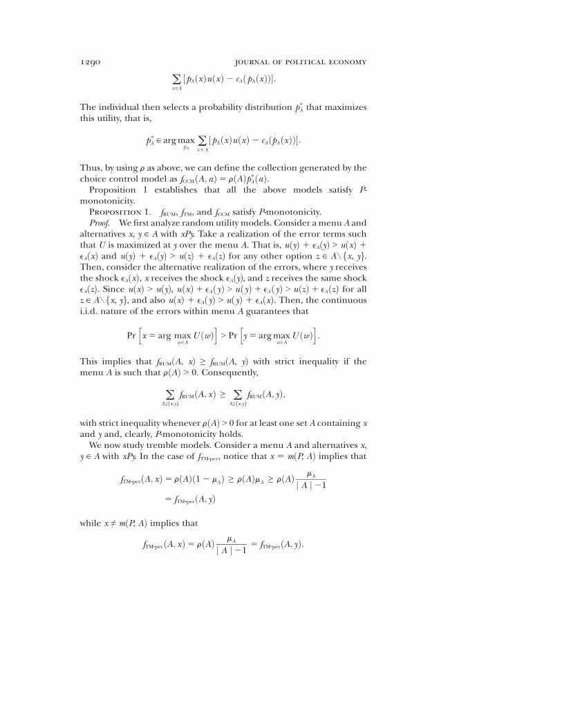
Thus, by using r as above, we can define the collection generated by thechoice control model as fCCMðA; aÞ5 rðAÞp*AðaÞ.Proposition 1 establishes that all the above models satisfy P-

monotonicity.Proposition 1. fRUM, fTM, and fCCM satisfy P-monotonicity.Proof. We first analyze random utility models. Consider a menu A and

alternatives x, y ∈ A with xPy. Take a realization of the error terms suchthat U is maximized at y over the menu A. That is, uðyÞ 1 eAðyÞ > uðxÞ 1eAðxÞ and uðyÞ 1 eAðyÞ > uðzÞ 1 eAðzÞ for any other option z ∈ A /fx, yg.Then, consider the alternative realization of the errors, where y receivesthe shock eAðxÞ, x receives the shock eAðyÞ, and z receives the same shockeAðzÞ. Since uðxÞ > uðyÞ, uðxÞ1 eAðyÞ > uðyÞ1 eAðyÞ > uðzÞ1 eAðzÞ for allz ∈ A /fx, yg, and also uðxÞ 1 eAðyÞ > uðyÞ 1 eAðxÞ. Then, the continuousi.i.d. nature of the errors within menu A guarantees that

Prhx 5 arg max

w∈AU ðwÞ

i> Pr

hy 5 argmax

w∈AU ðwÞ

i:

This implies that fRUMðA, xÞ ≥ fRUMðA, yÞ with strict inequality if themenu A is such that rðAÞ > 0. Consequently,

oA⊇fx;yg

fRUMðA; xÞ ≥ oA⊇fx;yg

fRUMðA; yÞ;

with strict inequality whenever rðAÞ > 0 for at least one set A containing xand y and, clearly, P-monotonicity holds.We now study tremble models. Consider a menu A and alternatives x,

y ∈ A with xPy. In the case of fTM-per, notice that x 5 mðP, AÞ implies that

fTM-perðA; xÞ5 rðAÞð12 mAÞ ≥ rðAÞmA ≥ rðAÞ mA

j A j21

5 fTM-perðA; yÞ

while x ≠ mðP, AÞ implies that

fTM-perðA; xÞ5 rðAÞ mA

j A j215 fTM-perðA; yÞ:


In the case of fTM-pro, if y is not the worst alternative in A,

fTM-proðA; xÞ5 rðAÞð12 mAÞmjfz∈A:z PxgjA ≥ rðAÞð12 mAÞmjfz∈A:z Pygj

A

5 fTM-proðA; yÞ:

If y is the worst alternative in A,

fTM-proðA; xÞ5 rðAÞð12 mAÞmjfz∈A:zPxgjA ≥ rðAÞmjAj21

A

5 fTM-proðA; yÞ:

Then

oA⊇fx;yg

fTMðA; xÞ ≥ oA⊇fx;yg

fTMðA; yÞ;

with strict inequality whenever rðAÞ > 0 for at least one set A such thatðiÞ in the case of fTM-per, x is the best alternative in A ⊇ fx, yg, and ðiiÞ in thecase of fTM-pro, A ⊇ fx, yg. This is clearly the case for fx, yg, and hence P-monotonicity holds.Finally, we analyze choice control models. Consider a menu A and

alternatives x, y ∈ A with xPy. We first prove that fCCMðA, xÞ ≥ fCCMðA, yÞ.Suppose, by contradiction, that fCCMðA, xÞ < fCCMðA, yÞ or, equivalently,p*AðxÞ < p*AðyÞ. Consider p0

A with p0AðxÞ5 p*AðyÞ, p0

AðyÞ5 p*AðxÞ, and p0AðzÞ5

p*AðzÞ for all z ∈ A /fx, yg. Since, by assumption, uðxÞ > uðyÞ, it is the casethat

ow∈A

½p0AðwÞuðwÞ2 cAðp0

AðwÞÞ� > ow∈A

½p*AðwÞuðwÞ2 cAðp*AðwÞÞ�;

thus contradicting the optimality of p*. Since this is true for every menu,

oA⊇fx;yg

fCCMðA; xÞ ≥ oA⊇fx;yg

fCCMðA; yÞ

holds. For the strict part, notice that continuity of cfx,yg prevents the opti-mal solution p* from being constant in fx, yg, and hence P-monotonicityfollows. QEDWe now show that the swaps index always identifies the true under-

lying preference in models that satisfy P-monotonicity and, particularly,that the presence of all the menus in the data guarantees that the swapsindex uniquely identifies the preference.Theorem 1. If f satisfies P-monotonicity, then P is a swaps prefer-

ence of f. If, moreover, oa∈Af ðA; aÞ > 0 holds for every menu A, then P isthe unique swaps preference of f.


Proof. Let f be P-monotone. Consider any preference P0 different

from P. Then, there exist at least two alternatives a1 and a2 that areconsecutive in P

0, with a2P0a1 but a1Pa 2. Define a new preference P

00 byxP

00y ⇔ xP0y whenever fx, yg ≠ fa1, a2g and a1P

00a2. That is, P

00 is simplydefined by changing the position of the consecutive alternatives a1 anda2 in P

0, reconciling their comparison with that of preference P andleaving all else the same. We now show that P 00 rationalizes data withfewer swaps than P 0. To see this, simply notice that the swaps computa-tion will be affected only by menus A such that A ⊇ fa1, a 2g. Also, for anyof such sets, since both alternatives are consecutive in both P

0 and P00, the

swaps computation will be affected only by observations of the formðA, a1Þ and ðA, a 2Þ and clearly,

oðA;aÞ

f ðA; aÞ j fx ∈ A : xP 00ag j 5 oðA;aÞ

f ðA; aÞ j fx ∈ A : xP 0ag j

1 oA⊇fa1;a 2g

f ðA; a2Þ2 oA⊇fa1;a 2g

f ðA; a1Þ:

Since f is P-monotone, the latter is smaller than or equal tooðA;aÞ f ðA; aÞ j fx ∈ A : xP 0ag j, as desired. Given the finiteness of X, re-peated application of this algorithm leads to preference P and provesthat

oðA;aÞ

f ðA; aÞ j fx ∈ A : xPag j ≤ oðA;aÞ

f ðA; aÞ j fx ∈ A : xP 0ag j :

Hence, P is an argument that minimizes the swaps index. Wheneveroa∈Af ðA; aÞ > 0 holds for every menu A, it is in particular satisfied for themenus fa1, a 2g involved in each step of the previous algorithm. By P-monotonicity, the corresponding inequalities are strict, and therefore Pis the unique swaps preference. QEDTheorem 1 provides a simple test to guarantee that the swaps index

identifies the true preference of a particular choice model. Two ques-tions naturally arise at this point. The first is whether other indices mayalso systematically recover it when P-monotonicity holds. It is easy to seethat the Afriat and Varian indices do not possess this recovery propertyin general, since they depend on the monetary structure of the alter-natives, which is not necessarily aligned with preferences. To see this,consider the simplest case in which X 5 fx, yg and suppose xPy. Noticethat if f ðX, yÞ ≠ 0, IA recovers P if and only if wX

x ≤ wXy . Similarly, IV re-

covers P if and only if wXx =w

Xy ≤ f ðX ; xÞ=f ðX ; yÞ. Without these extra con-

ditions, IA and IV are unable to recover P. Moreover, indices based on thenumber of violations of a rationality property, such as IW or the moneypump index, are also unable to recover the preference, since these in-


dices are not built to identify any particular preference, nor can they bewritten in this form.16 Finally, since IHM does not take into considerationthe severity of the inconsistencies, it is also unable to recover P from P-monotone models. To see this, let X5 fx, y, zg with xPyPz, and consider amodel generating a P-monotone collection f such that f ðfy, zg, yÞ < f ðfy,zg, zÞ. It is immediate that the mass of inconsistent observations in f withrespect to xP

0zP

0y is strictly lower than that of P, and hence the optimal

preference for IHM cannot be P.17

The next question concerns choice models not satisfying P-monotonicityfor which IS does not recover the true preference. A leading case is con-sideration set models.18 In this setting, the individual considers each alter-native with a given probability and then chooses the maximal alternativefrom those that have been considered, and hence good alternatives maybe chosen with low probability. We can address this case by using a slightgeneralization of IS, the nonneutral swaps index INNS proposed in Sec-tion VI.B.

V. Axiomatic Foundations for the Swaps Index

Here, we propose seven properties that shape the way in which an in-consistency index I treats different types of collections of observations.We then show that the swaps index is characterized by this set of prop-erties.Continuity ðCONTÞ.—The index I is a continuous function. That is,

for every sequence f fng ⊆ F , if fn → f, then Ið fnÞ → Ið f Þ.This is the standard definition of continuity, which is justified in the

standard fashion. That is, it is desirable that a small variation in the datadoes not cause an abrupt change in the inconsistency value.Rationality ðRAT Þ.—For every f ∈ F , Ið f Þ 5 0 if and only if f is ratio-

nalizable.Rationality imposes that a collection of observations is perfectly con-

sistent if and only if the collection is rationalizable. In line with themaximization principle, rationality establishes that the minimal incon-sistency level of 0 is reached only when every single choice in the col-lection can be explained by maximizing the same preference relation.Concavity ðCONCÞ.—The index I is a concave function. That is, for

every f, g ∈ F and every a ∈ ½0, 1�,

16 In Sec. V we discuss the axiom piecewise linearity, which allows for the recoverability ofpreferences.

17 Again, in Sec. V we discuss the axiom disjoint composition, which allows us to accountfor the severity of the inconsistencies.

18 See Masatlioglu et al. ð2012Þ for a deterministic modeling and Manzini and Mariottið2014Þ for a recent stochastic model.


I ðaf 1 ð12 aÞg Þ ≥ aI ð f Þ1 ð12 aÞI ðg Þ:.To illustrate the desirability of this property in our context, take any

two collections f and g and suppose them to be rationalizable whentaken separately. Clearly, a convex combination of f and g does not needto be rationalizable, and hence the collection af1 ð12 aÞg can take onlythe same or a higher inconsistency value than the combination of theinconsistency values of the two collections. The same idea applies wheneither f or g or both are not rationalizable. The combination of f and gcan generate the same or a greater number of frictions only with themaximization principle and hence should yield the same or a higherinconsistency value.Piecewise linearity ðPWLÞ.—The index I is a piecewise linear function

over jPj pieces. That is, there are jPj subsets of F , the union of whichis F such that for every pair f, g belonging to the same subset and everya ∈ ½0, 1�,

I ðaf 1 ð12 aÞg Þ5 aI ð f Þ1 ð12 aÞI ðg Þ:

Piecewise linearity brings two features: the piecewise nature of theindex and the linear structure of the index over each piece. Let us nowelaborate on the desirability of these two features.Notice that the piecewise assumption in piecewise linearity is attractive

from the recoverability of preferences perspective and hence is criticalfor predicting behavior and enabling individual welfare analysis. An in-dex satisfying the piecewise assumption divides the set of collectionsof observations F into jPj classes. Thus, as any preference is linked toone and only one of such classes, every single collection of observations,even the nonrationalizable ones, can be linked to a specific preferencerelation.Within each of the pieces, piecewise linearity makes the index react

monotonically with respect to inconsistencies, whether they are ðiÞ of thesame type, thus making the index react to the mass of an inconsistency,or ðiiÞ of different types, thus making the index react to the accumula-tion of several different inconsistencies. To enable formal study of theseimplications, we introduce a useful class of collections of observations,which we describe as perturbed. Consider a rationalizable collection ofobservations r ∈ R and an observation ðA, aÞ ∈ O. An e-perturbation of rin the direction of ðA, aÞ involves replacing an e-mass of optimal choicesðA, mðP r, AÞÞ with the possibly suboptimal choices ðA, aÞ.19 We denote

19 Obviously, the value of e must be lower than r ðA, mðP 0, AÞÞ.


such a perturbed collection by r eðA;aÞ 5 r 1 e1ðA;aÞ 2 e1ðA;mðPr ;AÞÞ and thecollection in which two different e-perturbations take place by

r eðA;aÞeðB;bÞ 5 r 1 e1ðA;aÞ 2 e1ðA;mðPr ;AÞÞ 1 e1ðB;bÞ 2 e1ðB;mðPr ;BÞÞ:

The following lemma, proved in Appendix A, establishes the above im-plications.Lemma 1. Let I be an inconsistency index satisfying PWL, CONT,

and RAT. Consider any collection r ∈ R and any two different obser-vations ðA, aÞ, ðB, bÞ such that a ≠ mðP r, AÞ and b ≠ mðP r, BÞ. For any twosufficiently small real values e1 > e2 ≥ 0,

1. reactivity to the mass of an inconsistency: I ðr e1ðA;aÞÞ > I ðr e2ðA;aÞÞ;2. reactivity to several inconsistencies: I ðr e1ðA;aÞe1ðB;bÞ Þ >maxfI ðr e1ðA;aÞÞ;

I ðr e1ðB;bÞÞg.The proof of lemma 1 explicitly shows how PWL implies reactivity

of the index to both the mass and the types of inconsistencies in a lin-ear fashion, namely, I ðr e1ðA;aÞÞ5 ðe1=e2ÞI ðr e2ðA;aÞÞ and I ðr e1ðA;aÞe1ðB;bÞ Þ5 I ðr e1ðA;aÞÞ1I ðr ε1ðB;bÞÞ.Ordinal consistency ðOCÞ.—For every ðA, aÞ ∈ O and every r, ~r ∈R such

that r ðfx; yg; xÞ5 ~r ðfx; yg; xÞ whenever x, y ∈ A, it is I ðr eðA;aÞÞ5 I ð~r eðA;aÞÞ forany sufficiently small e > 0.Ordinal consistency is in the spirit of the classical properties of in-

dependence of irrelevant alternatives. A small perturbation of the typeðA, aÞ generates the same inconsistency in two rationalizable collections rand ~r that coincide in the ranking of the alternatives within A but maydiverge in the ranking of alternatives outside A. In other words, theorder of alternatives not involved in the inconsistency is inconsequen-tial. In line with the standard justification for such a property, one maysimply contend that when evaluating a perturbed collection, any alter-native not involved in the perturbation at hand should not matter.Disjoint composition ðDCÞ.—For every ðA1, aÞ, ðA2, aÞ ∈ O such that A1 \

A2 5 fag and every r ∈ R, it is I ðr eðA1[A2;aÞÞ5 I ðr eðA1;aÞeðA2;aÞ Þ for any sufficiently

small e > 0.In words, disjoint composition states that, given a rationalizable col-

lection r, a small perturbation of the type ðA1 [ A2, aÞ can be brokendown into two small perturbations of the form ðA1, aÞ and ðA2, aÞ, pro-vided that A1 and A2 share no alternative other than a. By iteration, anindex having this property is able to reduce the inconsistency of theobservation into inconsistencies involving binary comparisons. Thisproperty is desirable for several reasons. First, from a purely normativepoint of view, notice that the standard welfare approach is constructedprecisely on the basis of binary comparisons. Hence, an index that aimsto capture the severity of an inconsistency in terms of the welfare loss


involved must likewise be based on binary comparisons. Second, from apractical point of view, this decomposition facilitates the tractability ofthe data by compacting it into a unique matrix of binary choices. Toillustrate, notice that both r eðA1[A2;aÞ and r eðA1;aÞ

eðA2;aÞ correspond to the follow-ing summary of binary revealed choices. Whenever xPra and x ∈ A1 [ A2,e percent of the data is inconsistent with x being preferred to a. Noinconsistencies arise in any other comparison of two alternatives. Dis-joint composition implies that this summary is the only relevant infor-mation and hence declares the two collections equally inconsistent.In order to introduce our last property, let us consider the follow-

ing notation. Given a permutation j over the set of alternatives X, forany collection f we denote by jð f Þ the permuted collection such thatjð f ÞðA, aÞ 5 f ðjðAÞ, jðaÞÞ.Neutrality ðNEU Þ.—For every permutation j and every f ∈ F , Ið f Þ 5

Iðjð f ÞÞ.Neutrality imposes that the inconsistency index should be indepen-

dent of the names of the alternatives. That is, any relabeling of thealternatives should have no effect on the level of inconsistency.Theorem 2 states the characterization result.Theorem 2. An inconsistency index I satisfies CONT, RAT, CONC,

PWL, OC, DC, and NEU if and only if it is a positive scalar transforma-tion of the swaps index.Proof. It is immediate to see that any positive scalar transformation of

the swaps index satisfies the axioms. By way of seven steps, we show thatan index satisfying the axioms is a transformation of the swaps index.Step 1: Following the proof of lemma 1, consider the convex hulls of

the closure of the jPj subsets of collections. Reasoning analogously, forevery r ∈ R, there exists ar ∈ ð0, 1Þ such that, for every observation ðA, aÞand every a ∈ ½0, ar �, the collection a1ðA,aÞ 1 ð1 2 aÞr belongs to theconvex hull of r. We then define, for every r and ðA, aÞ, the weight

wðP r ;A; aÞ5 I ðar1ðA;aÞ 1 ð12 ar Þr Þar

:

Now notice that, whenever aPrx for all x ∈ A /fag, the collection ar1ðA,aÞ 1ð1 2 arÞr is rationalizable by P r and RAT implies wðP r, A, aÞ 5 0. Oth-erwise, it follows that rðA, xÞ > 0 with x ≠ a, which implies that obser-vations ðA, aÞ and ðA, xÞ have positive mass in the collection ar1ðA,aÞ 1ð1 2 ar Þr, and RAT guarantees that wðP r, A, aÞ > 0.Step 2: We now prove that, whenever f ∈ F and r ∈ R belong to the

same convex hull, it is the case that I ð f Þ5oðA;aÞf ðA; aÞwðP r ;A; aÞ. ByRAT and PWL,


I ð f Þ5 ar I ð f Þar

5ar I ð f Þ1 ð12 ar ÞI ðr Þ

ar5

I ðar f 1 ð12 ar Þr Þar

:

Notice that

ar f 1 ð12 ar Þr 5 ar

�oðA;aÞ

f ðA; aÞ1ðA;aÞ

�1 ð12 ar Þr

5 oðA;aÞ

f ðA; aÞ½ar1ðA;aÞ 1 ð12 ar Þr �:

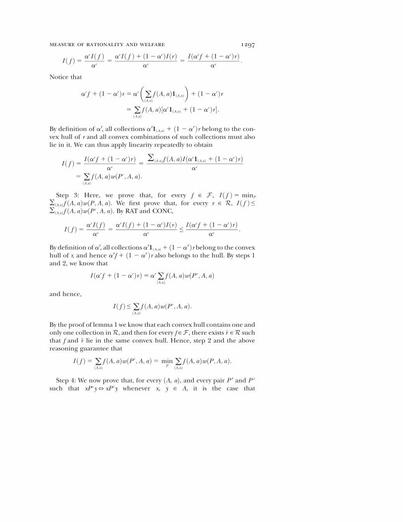
By definition of ar, all collections ar1ðA,aÞ 1 ð1 2 arÞr belong to the con-vex hull of r and all convex combinations of such collections must alsolie in it. We can thus apply linearity repeatedly to obtain

I ð f Þ5 I ðar f 1 ð12 ar Þr Þar

5oðA;aÞf ðA; aÞI ðar1ðA;aÞ 1 ð12 ar Þr Þ

ar

5 oðA;aÞ

f ðA; aÞwðP r ;A; aÞ:

Step 3: Here, we prove that, for every f ∈ F , I ð f Þ5 minP

oðA;aÞf ðA; aÞwðP ;A; aÞ. We first prove that, for every r ∈ R, I ð f Þ ≤oðA;aÞf ðA; aÞwðP r ;A; aÞ. By RAT and CONC,

I ð f Þ5 ar I ð f Þar

5ar I ð f Þ1 ð12 ar ÞI ðr Þ

ar≤I ðar f 1 ð12 ar Þr Þ

ar:

By definition of ar, all collections ar1ðA,aÞ1 ð12 arÞr belong to the convexhull of r, and hence arf 1 ð1 2 ar Þr also belongs to the hull. By steps 1and 2, we know that

I ðar f 1 ð12 ar Þr Þ5 ar oðA;aÞ

f ðA; aÞwðP r ;A; aÞ

and hence,

I ð f Þ ≤ oðA;aÞ

f ðA; aÞwðP r ;A; aÞ:

By the proof of lemma 1 we know that each convex hull contains one andonly one collection inR, and then for every f ∈ F , there exists r ∈R suchthat f and r lie in the same convex hull. Hence, step 2 and the abovereasoning guarantee that

I ð f Þ5 oðA;aÞ

f ðA; aÞwðP r ;A; aÞ5 minP o

ðA;aÞf ðA; aÞwðP ;A; aÞ:

Step 4: We now prove that, for every ðA, aÞ, and every pair P r and P ~r

such that xP r y⇔ xP ~r y whenever x, y ∈ A, it is the case that


wðP r ;A; aÞ5 wðP ~r ;A; aÞ. To see this, notice that there exists a sufficientlysmall a such that raðA,aÞ and ~r aðA;aÞ belong to the convex hulls of r and ~r ,respectively. By steps 1 and 2 and OC, it is the case that

awðP r ;A; aÞ5 I ðr aðA;aÞÞ5 I ð~r aðA;aÞÞ5 awðP ~r ;A; aÞor, equivalently, wðP r ;A; aÞ5 wðP ~r ;A; aÞ.Step 5: Here we prove that, for every ðA, aÞ and Pr, wðP r ;A; aÞ5

ox∈AwðP r ; fx; ag; aÞ. To do this, we prove that for any two menus A1,A2 such that A1 \ A2 5 fag and A1 [ A2 5 A, it is the case thatwðP r ;A; aÞ5 wðP r ;A1; aÞ1 wðP r ;A2; aÞ. The recursive application of thisidea, given the finiteness of X, concludes the step. Again, there exists asufficiently small a such that raðA,aÞ, r aðA1;aÞ, and r aðA2;aÞ all belong to theconvex hull of r. By steps 1 and 2 and DC, it is the case that

awðP r ;A; aÞ5 I ðr aðA;aÞÞ5 I ðr aðA1;aÞaðA2;aÞ Þ

5 awðP r ;A1; aÞ1 awðP r ;A2; aÞ;which implies wðP r ;A; aÞ5 wðP r ;A1; aÞ1 wðP r ;A2; aÞ.Step 6: Here we prove that wðP r ; fx; yg; yÞ5 wðP ~r ; fz; tg; tÞ holds for

every x, y, z, t ∈ X and every pair Pr and P ~r such that the ranking of xðrespectively, of yÞ in Pr is the same as the ranking of z ðrespectively, of tÞin P ~r . Consider the bijection j : X → X, which assigns, to the alternativeranked at s in Pr, the alternative ranked at s in P ~r . Then, it is jðxÞ 5 zand jðyÞ 5 t and also, jðr Þ5 ~r . There exists a sufficiently small a suchthat raðfx,yg,yÞ belongs to the convex hull of r and ~r aðfz;tg;tÞ belongs to theconvex hull of ~r . By steps 1 and 2 and NEU, we have that

awðP r ; fx; yg; yÞ5 I ðr aðfx;yg;yÞÞ5 I ðjðr aðfx;yg;yÞÞÞ5 I ð~r aðfz;tg;tÞÞ5 awðP ~r ; fz; tg; tÞ;

that is, wðP r ; fx; yg; yÞ5 wðP ~r ; fz; tg; tÞ.Step 7: We finally prove that I is a positive scalar transformation of the

swaps index. Let P and P 0 be any two preferences and consider x, y, z, t ∈ Xwith xPy and zP 0t. Thanks to step 4, consider without loss of generality thatx and y ðrespectively, z and tÞ are the first two elements of P ðrespectively,P 0Þ. Steps 1 and 6 guarantee that wðP ; fx; yg; yÞ5 wðP 0; fz; tg; tÞ > 0 andsteps 3 and 5 lead to

I ð f Þ5 minP o

ðA;aÞf ðA; aÞwðP ;A; aÞ

5 minP o

ðA;aÞf ðA; aÞ o

x∈A:xPawðP ; fx; ag; aÞ

5 K minP o

ðA;aÞf ðA; aÞ j fx ∈ A : xPag j;


with K > 0, which shows that I is a positive scalar transformation of theswaps index. QEDTable 1 illustrates the structural relationship of the swaps index with

the other rationality indices discussed in Section III.A. We do this bystating which axioms, among those characterizing the swaps index, theysatisfy.

VI. A General Class of Indices

A. General Weighted Index

The swaps index relies exclusively on the endogenous information con-tained in the revealed choices. On occasions, however, the analyst mayhave more information and may wish to use it to assess the consistencyof choice and identify the optimal welfare ranking. We now offer a gen-eralization of the swaps index that is able to incorporate other informa-tion. The general weighted index considers every possible inconsistency be-tween an observation and a preference relation through a weight thatmay depend on the nature of the menu of alternatives, the nature of thechosen alternative, and the nature of the preference relation. Then, fora given collection f, the inconsistency index takes the form of the mini-mum total inconsistency across all preference relations:

IGð f Þ5 minP o

ðA;aÞf ðA; aÞwðP ;A; aÞ;

where wðP, A, aÞ 5 0 if a 5 mðP, AÞ and wðP, A, aÞ ∈ R11 otherwise.It turns out that the general weighted index is characterized by the first

four axioms used in the characterization of the swaps index.20

Proposition 2. An inconsistency index I satisfies CONT, RAT, CONC,and PWL if and only if it is a general weighted index.

TABLE 1Summary of the Relationship between Axioms and Inconsistency Indices

CONT RAT CONC PWL OC NEU DC

IS ✓ ✓ ✓ ✓ ✓ ✓ ✓IHM ✓ ✓ ✓ ✓ ✓ ✓ XIV ✓ ✓ ✓ ✓ ✓ X XIW ✓ ✓ ✓a X X ✓ XIW2MP ✓ ✓ ✓a X X X XIA X ✓ ✓ X X X X

a IW and IW2MP do not satisfy CONC, but a simple transformation would do. SeeSec. VII for how to build the transformation in an application.

20 The proof of this result, and all the ones that follow, can be found in App. A.


B. Nonneutral Swaps Index and Positional Swaps Index

We now present two indices from the class of general weighted indicesthat may be especially relevant. We start by considering settings in whichthe analyst has information on the nature of the alternatives, such as theirmonetary values, attributes, and so forth. Under these circumstances, theproperty of NEU may lose its appeal, since one now may wish to treatdifferent pairs of alternatives differently, using the exogenous informa-tion that is available on them. It turns out that the remaining six prop-erties in theorem 2 characterize a class of indices that we call the non-neutral swaps index. Let wx,a ∈ R11 denote the weight of the ordered pairof alternatives x and a; that is, wx,a represents the cost of swapping thepreferred alternative x with the chosen alternative a. Then

INNSð f Þ5 minP o

ðA;aÞf ðA; aÞ o

x∈A:xPawx;a :

Proposition 3. An inconsistency index I satisfies CONT, RAT, CONC,PWL, OC, and DC if and only if it is a nonneutral swaps index.Now suppose that the analyst has information on the cardinal utility

values of the different alternatives, based on their position in the rank-ing, and wants to use it. Then, OC, which completely disregards this typeof information, immediately obliterates its appeal. We show that the elim-ination of OC from the system of properties characterizes the followingindex, which we call the positional swaps index:

IPSð f Þ5 minP o

ðA;aÞf ðA; aÞ o

x∈A:xPawxðP Þ;aðP Þ;

where wi,j ∈ R11 denotes the weight associated with positions i and j andxðP Þ is the ranking of alternative x in P. Again, wi,j is interpreted as thecost of swapping the preferred alternative, the one that occupies posi-tion i in the ranking, with the chosen alternative, that occupies positionj in the ranking.Proposition 4. An inconsistency index I satisfies CONT, RAT, CONC,

PWL, DC, and NEU if and only if it is a positional swaps index.

C. Varian and Houtman-Maks

As introduced in Section III.A, two popular measures of the consistencyof behavior are due to Varian ð1990Þ and Houtman and Maks ð1985Þ.We have already shown that these indices satisfy the properties that, bytheorem 3, characterize the general weighted indices. We now providetheir complete characterizations.Let us start with the case of Varian. Its characterization requires a struc-

ture related to the search for themaximumweight in a given upper contour


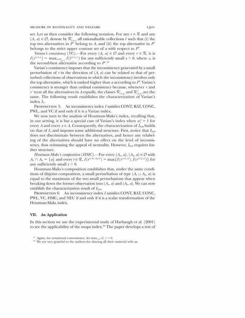
set. Let us then consider the following notation. For any r ∈ R and anyðA, aÞ ∈ O, denote by Rr

ðA;aÞ all rationalizable collections ~r such that ðiÞ thetop two alternatives in P ~r belong to A, and ðiiÞ the top alternative in P ~r

belongs to the strict upper contour set of a with respect to Pr.Varian’s consistency ðVCÞ.—For every ðA, aÞ ∈ O and every r ∈ R, it is

I ðr eðA;aÞÞ5 max~r ∈RrðA;aÞ

I ð~r eðA;z~r ÞÞ for any sufficiently small e > 0, where z~r isthe second-best alternative according to P ~r .21

Varian’s consistency imposes that the inconsistency generated by a smallperturbation of r in the direction of ðA, aÞ can be related to that of per-turbed collections of observations in which the inconsistency involves onlythe top alternative, which is ranked higher than a according to Pr. Varian’sconsistency is stronger than ordinal consistency because, whenever r andr 0 treat all the alternatives in A equally, the classesRr

ðA;aÞ andRr 0ðA;aÞ are the

same. The following result establishes the characterization of Varian’sindex IV.Proposition 5. An inconsistency index I satisfies CONT, RAT, CONC,

PWL, and VC if and only if it is a Varian index.We now turn to the analysis of Houtman-Maks’s index, recalling that,

in our setting, it is but a special case of Varian’s index when wAx 5 1 for

every A and every x ∈ A. Consequently, the characterization of IHM buildson that of IV and imposes some additional structure. First, notice that IHM

does not discriminate between the alternatives, and hence any relabel-ing of the alternatives should have no effect on the level of inconsis-tency, thus reinstating the appeal of neutrality. However, IHM requires fur-ther structure.Houtman-Maks’s composition ðHMCÞ.—For every ðA1, aÞ, ðA2, aÞ ∈ O with

A1 \ A2 5 fag and every r ∈R, I ðr eðA1[A2;aÞÞ5maxfI ðr eðA1;aÞÞ; I ðr eðA2;aÞÞg forany sufficiently small e > 0.Houtman-Maks’s composition establishes that, under the same condi-

tions of disjoint composition, a small perturbation of type ðA1 [ A2, aÞ isequal to the maximum of the two small perturbations that appear whenbreaking down the former observation into ðA1, aÞ and ðA2, aÞ. We can nowestablish the characterization result of IHM.Proposition 6. An inconsistency index I satisfies CONT, RAT, CONC,

PWL, VC, HMC, and NEU if and only if it is a scalar transformation of theHoutman-Maks index.

VII. An Application

In this section we use the experimental study of Harbaugh et al. ð2001Þto see the applicability of the swaps index.22 The paper develops a test of

21 Again, for notational convenience, let maxr ∈∅ I ð� Þ5 0.22 We are very grateful to the authors for sharing all their material with us.


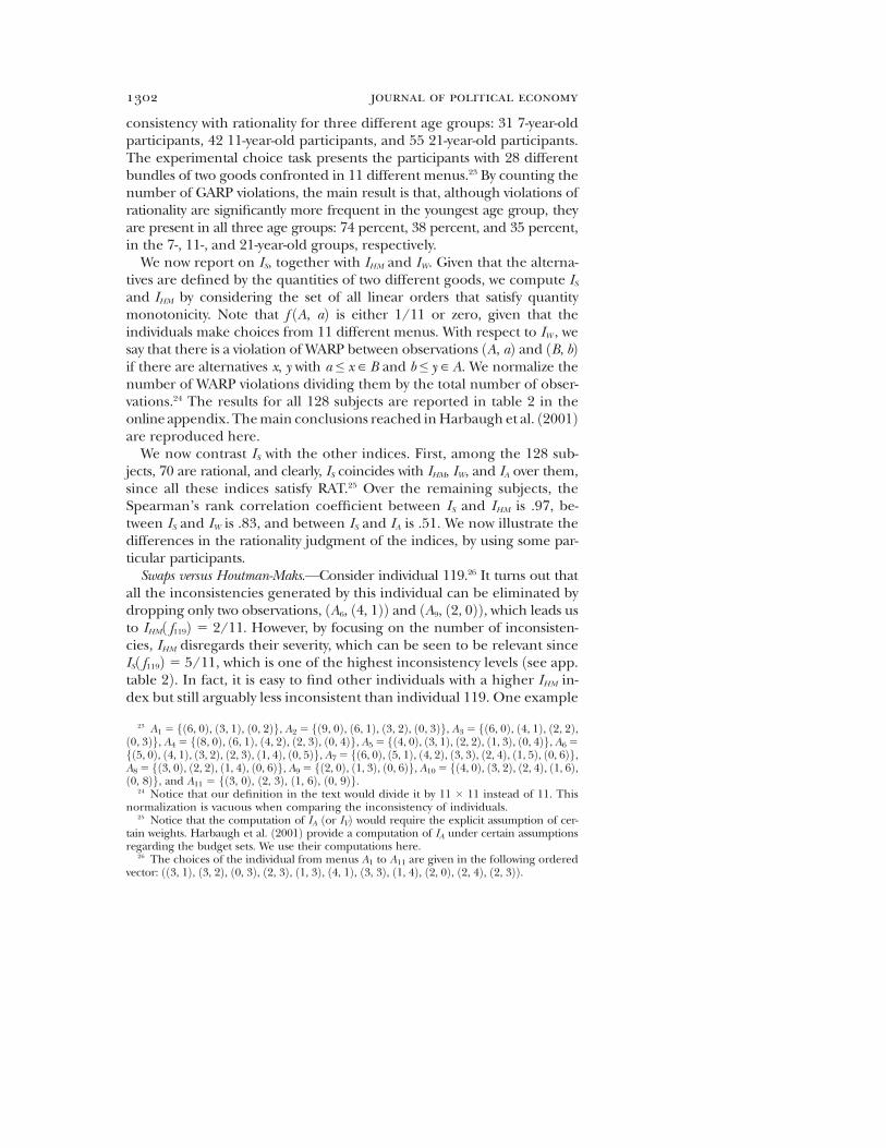
consistency with rationality for three different age groups: 31 7-year-oldparticipants, 42 11-year-old participants, and 55 21-year-old participants.The experimental choice task presents the participants with 28 differentbundles of two goods confronted in 11 different menus.23 By counting thenumber of GARP violations, the main result is that, although violations ofrationality are significantly more frequent in the youngest age group, theyare present in all three age groups: 74 percent, 38 percent, and 35 percent,in the 7-, 11-, and 21-year-old groups, respectively.We now report on IS, together with IHM and IW. Given that the alterna-

tives are defined by the quantities of two different goods, we compute ISand IHM by considering the set of all linear orders that satisfy quantitymonotonicity. Note that f ðA, aÞ is either 1/11 or zero, given that theindividuals make choices from 11 different menus. With respect to IW , wesay that there is a violation of WARP between observations ðA, aÞ and ðB, bÞif there are alternatives x, y with a ≤ x ∈ B and b ≤ y ∈ A. We normalize thenumber of WARP violations dividing them by the total number of obser-vations.24 The results for all 128 subjects are reported in table 2 in theonline appendix. Themain conclusions reached inHarbaugh et al. ð2001Þare reproduced here.We now contrast IS with the other indices. First, among the 128 sub-

jects, 70 are rational, and clearly, IS coincides with IHM, IW, and IA over them,since all these indices satisfy RAT.25 Over the remaining subjects, theSpearman’s rank correlation coefficient between IS and IHM is .97, be-tween IS and IW is .83, and between IS and IA is .51. We now illustrate thedifferences in the rationality judgment of the indices, by using some par-ticular participants.Swaps versus Houtman-Maks.—Consider individual 119.26 It turns out that

all the inconsistencies generated by this individual can be eliminated bydropping only two observations, ðA6, ð4, 1ÞÞ and ðA9, ð2, 0ÞÞ, which leads usto IHMð f119Þ 5 2/11. However, by focusing on the number of inconsisten-cies, IHM disregards their severity, which can be seen to be relevant sinceISð f119Þ 5 5/11, which is one of the highest inconsistency levels ðsee app.table 2Þ. In fact, it is easy to find other individuals with a higher IHM in-dex but still arguably less inconsistent than individual 119. One example

23 A1 5 fð6, 0Þ, ð3, 1Þ, ð0, 2Þg, A2 5 fð9, 0Þ, ð6, 1Þ, ð3, 2Þ, ð0, 3Þg, A3 5 fð6, 0Þ, ð4, 1Þ, ð2, 2Þ,ð0, 3Þg, A45 fð8, 0Þ, ð6, 1Þ, ð4, 2Þ, ð2, 3Þ, ð0, 4Þg, A55 fð4, 0Þ, ð3, 1Þ, ð2, 2Þ, ð1, 3Þ, ð0, 4Þg, A65fð5, 0Þ, ð4, 1Þ, ð3, 2Þ, ð2, 3Þ, ð1, 4Þ, ð0, 5Þg, A75 fð6, 0Þ, ð5, 1Þ, ð4, 2Þ, ð3, 3Þ, ð2, 4Þ, ð1, 5Þ, ð0, 6Þg,A85 fð3, 0Þ, ð2, 2Þ, ð1, 4Þ, ð0, 6Þg, A95 fð2, 0Þ, ð1, 3Þ, ð0, 6Þg, A105 fð4, 0Þ, ð3, 2Þ, ð2, 4Þ, ð1, 6Þ,ð0, 8Þg, and A11 5 fð3, 0Þ, ð2, 3Þ, ð1, 6Þ, ð0, 9Þg.

24 Notice that our definition in the text would divide it by 11 � 11 instead of 11. Thisnormalization is vacuous when comparing the inconsistency of individuals.

25 Notice that the computation of IA ðor IVÞ would require the explicit assumption of cer-tain weights. Harbaugh et al. ð2001Þ provide a computation of IA under certain assumptionsregarding the budget sets. We use their computations here.

26 The choices of the individual from menus A1 to A11 are given in the following orderedvector: ðð3, 1Þ, ð3, 2Þ, ð0, 3Þ, ð2, 3Þ, ð1, 3Þ, ð4, 1Þ, ð3, 3Þ, ð1, 4Þ, ð2, 0Þ, ð2, 4Þ, ð2, 3ÞÞ.


is subject 60, who presents threemild inconsistencies, and IHMð f60Þ5 3/115ISð f60Þ.27Swaps versus WARP.—Individual 28, with IWð f28Þ5 6/11, represents one of

the cases with the largest number of cycles.28 However, by merely count-ing the number of cycles, IW is unable to determine the number and se-verity of the mistakes that need to be cancelled in order to break the cycles.Closer inspection shows that this can be done by eliminating only two mildinconsistencies. This is what the swaps index does, ISð f28Þ 5 2/11, with in-consistent observations ðA4, ð2, 3ÞÞ and ðA11, ð3, 0ÞÞ, where, according to PS,only ð4, 2Þ is preferred to ð2, 3Þ in the first and ð2, 3Þ ranks above ð3, 0Þin the second. In this respect, there are a number of individuals that areclassed by IW as less inconsistent than individual 28 but whose choicesare nevertheless harder to reconcile with preference maximization, andwhose inconsistency values in terms of IS are therefore higher.Swaps versus Afriat.—Consider subject 12, who according to Afriat has a

relatively low inconsistency index, IAð f12Þ 5 .125.29 By considering onlythe largest violation and, within it, focusing on nonwelfare information,Afriat ignores ðiÞ that individual 12 commits a relatively large number ofmistakes ðthree, to be precise, since IHMð f12Þ 5 3/11Þ and ðiiÞ that the sub-ject is committing relatively serious mistakes by choosing alternatives thatare dominated by many others in the menu ðleading to ISð f12Þ 5 6/11Þ.Once again, it is easy to find cases that are incorrectly ordered by Afriat.Consider individual 28 or 119, for example, who requires larger incomeadjustments but, according to IS, fewer preference adjustments.

Appendix A

Remaining Proofs

Proof of Lemma 1

PWL guarantees that there are jPj pieces of F , over every one of which the in-dex is linear. The repeated application of linearity and CONT guarantee that theindex is also linear over the convex hull of the closure of each piece. We nowprove that each of these convex hulls contains one and only one collection inR.Suppose, by contradiction, that this is not the case. Since jPj 5 jRj, there mustexist two distinct r, r 0 belonging to the same convex hull. Then, PWL and RAT

27 The choices of individual 60 are ðð3, 1Þ, ð3, 2Þ, ð2, 2Þ, ð4, 2Þ, ð3, 1Þ, ð4, 1Þ, ð4, 2Þ, ð2, 2Þ,ð2, 0Þ, ð3, 2Þ, ð3, 0ÞÞ.

28 The choices of individual 28 are ðð3, 1Þ, ð9, 0Þ, ð2, 2Þ, ð2, 3Þ, ð2, 2Þ, ð3, 2Þ, ð3, 3Þ, ð2, 2Þ,ð2, 0Þ, ð3, 2Þ, ð3, 0ÞÞ.

29 The choices of individual 12 are ðð3, 1Þ, ð3, 2Þ, ð2, 2Þ, ð2, 3Þ, ð3, 1Þ, ð3, 2Þ, ð3, 3Þ, ð0, 6Þ,ð1, 3Þ, ð3, 2Þ, ð3, 0ÞÞ. Afriat’s inconsistency is driven by the critical observation ðA4, ð2, 3ÞÞ,where ð3, 2Þ is feasible and costs .875 times as much as the chosen element ð2, 3Þ, and in itscounterpart ðA10, ð3, 2ÞÞ, where ð2, 3Þ is feasible and costs .875 times as much as the chosenelement.


guarantee that, for every a ∈ ð0, 1Þ, it is the case that I ðar 1 ð12 aÞr 0Þ5 aI ðr Þ1ð12 aÞI ðr 0Þ5 0. However, since r ≠ r 0, there must exist at least one menu A andtwo distinct alternatives, a and b, such that rðA, aÞ > 0 and r 0ðA, bÞ > 0. Conse-quently, for a ∈ ð0, 1Þ, ½ar1 ð12 aÞr 0 �ðA, aÞ > 0 and ½ar1 ð12 aÞr 0 �ðA, bÞ > 0, andhence, ar 1 ð1 2 aÞr 0 is not rationalizable. RAT implies that Iðar 1 ð1 2 aÞr 0Þ ≠ 0,which is a contradiction. Now, given r and ðA, aÞ, the collections r eðA,aÞ converge tor as e goes to zero, and since there is a finite number of hulls, CONT guaranteesthat these collections belong to the same convex hull as r for sufficiently smallvalues of e. In the same vein, given r and two different observations ðA, aÞ and ðB, bÞ,the collections r and r eðA;aÞeðB;bÞ belong to the same convex hull for sufficiently smallvalues of e. Then, for sufficiently small perturbations e1 > e2 ≥ 0, PWL guaranteesthat

I ðr e2ðA;aÞÞ5 I�e2

e1r e1ðA;aÞ 1

�12

e2

e1

�r�5

e2

e1I ðr e1ðA;aÞÞ1

�12

e2

e1

�I ðr Þ:

Under the assumption of RAT, whenever a ≠ mðPr, AÞ, this is but

I ðr e2ðA;aÞÞ5 e2

e1I ðr e1ðA;aÞÞ < I ðr e1ðA;aÞÞ;

as desired. Now consider r, two different observations, ðA, aÞ and ðB, bÞ, and a suf-ficiently small perturbation e1 > 0. From PWL and the previous reasoning,

I ðr e1ðA;aÞe1ðB;bÞ Þ5 I�12r 2e1ðA;aÞ 1

12r 2e1ðB;bÞ

�5

12I ðr 2e1ðA;aÞÞ1 1

2I ðr 2e1ðB;bÞÞ

5 I ðr e1ðA;aÞÞ1 I ðr e1ðB;bÞÞ:

Whenever a ≠ mðPr, AÞ and b ≠ mðPr, BÞ, the latter is strictly larger thanmaxfI ðr e1ðA;aÞÞ; I ðr e1ðB;bÞÞg, as desired. QED

Proof of Proposition 2

Immediate from the proof of theorem 2. QED


It is easy to see that nonneutral swaps indices satisfy the axioms. To prove theconverse statement, we use steps 1–5 in the proof of theorem 2. By steps 1 and 5,

oðA;aÞ

f ðA; aÞwðP ;A; aÞ5 oðA;aÞ

f ðA; aÞ ox∈A:xPa

wðP ; fx; ag; aÞ:

By steps 1 and 4, wðP, fx, ag, aÞ > 0 is independent of P, provided that xPa, andthen we can write oðA;aÞf ðA; aÞox∈A:xPawx;a : Step 3 proves that the index is a non-neutral swaps index. QED



It is easy to see that positional swaps indices satisfy the axioms. To prove the con-verse, we use the proof of theorem 2 except steps 4 and 7. By steps 1 and 5,

oðA;aÞ

f ðA; aÞwðP ;A; aÞ5 oðA;aÞ

f ðA; aÞ ox∈A:xPa

wðP ; fx; ag; aÞ:

By steps 1 and 6, wðP, fx, ag, aÞ > 0 depends only on the rank of alternatives x anda in P. This, together with step 3, shows that the index is a positional swaps index.QED


It is easy to see that Varian’s index satisfies the axioms. For the converse, we usethe first three steps in the proof of theorem 2. Consider a set A, alternatives x, y,and z in A, and a pair, Pr and P �r , such that ðiÞ x and y are, respectively, the first-and second-best alternatives in Pr, and ðiiÞ x and z are, respectively, the first- andsecond-best alternatives in P �r . We claim that wðP r ;A; yÞ5 wðP �r ;A; zÞ. There exists asufficiently small a such that raðA,yÞ and �r aðA;zÞ belong, respectively, to the convexhulls of r and �r . Since the upper contour sets of y in Pr and z in P �r are both equalto fxg, it is the case that Rr

ðA;yÞ 5R�rðA;zÞ, and hence, steps 1 and 2 in the proof of

theorem 2 and VC imply

awðP r ;A; yÞ5 I ðr aðA;yÞÞ5 max~r ∈Rr

ðA;yÞ5 max

~r ∈R�rðA;zÞ

5 I ð�r aðA;zÞÞ

5 awðP �r ðA;zÞÞ:

We then denote this value by wAx . Now, given ðA, aÞ and r, there exists a sufficiently

small such that raðA,aÞ belongs to the convex hull of r and for every ~r ∈RrðA;aÞ, ~r

aðA;a~r Þ

belongs to the convex hull of ~r , where a~r is the second-best alternative in P ~r . Wecan apply steps 1 and 2 in the proof of theorem 2 andVC to see that

awðP r ;A; aÞ5 I ðr aðA;aÞÞ5 max~r ∈Rr

ðA;aÞI ð~r aðA;a~r ÞÞ5 max

~r ∈RrðA;aÞ

awðP ~r ;A; a~r Þ

5 a maxx∈A;xPr a

wAx :

This proves that the index is Varian’s index. QED


Clearly, Houtman-Maks’s index satisfies the axioms. To see the converse, fromthe proof of proposition 5, we now show that for every menu A and any pair ofalternatives x and y belonging to A, it is the case that wA

x 5 wfx;ygx . To see this,

consider any r such that x is the top alternative in Pr and y ∈ A is the second topalternative in Pr. For a sufficiently small a, it is the case that raðA,yÞ, raðfx,yg,yÞ, and


raðA /fyg,yÞ all belong to the convex hull of r. By steps 1 and 2 in the proof of theo-rem 2, HMC, and RAT, it is the case that

awAx 5 I ðr aðA;yÞÞ5maxfI ðr aðfx;yg;yÞ; I ðr aðA =fyg;yÞÞg5 I ðr aðfx;yg;yÞÞ5 awfx;yg

x :

NEU guarantees that wfx;ygx 5 wfz;tg

z for every x , y, z , t ∈ X , and given the strict positivityof these weights, the index is a scalar transformation of the Houtman-Maks index.QED

Appendix B

Uniqueness

Here we establish that almost all collections of observations have a unique swapspreference.

Proposition 7. The Lebesgue measure of the set of all collections of obser-

vations for which PS is not unique is zero.Proof. The set of all collections F is the simplex over all possible observations

ðA, aÞ. Consider two different preference relations, Pi and Pj , over X. We describethe set of collections F ij, for which the number of swaps associated with pref-erence Pi is equal to the number of swaps associated with preference Pj , that is,

oðA;aÞ

f ðA; aÞ j fx ∈ A : xPiag j 5 oðA;aÞ

f ðA; aÞ j fx ∈ A : xPjag j

or, equivalently,

oðA;aÞ

f ðA; aÞðj fx ∈ A : xPiag j 2 j fx ∈ A : xPjag jÞ5 0:

Consider the interior of the simplex F and notice that, since Pi and Pj aredifferent, there exists at least one observation such that ðj fx ∈ A : xPiag j 2j fx ∈ A : xPjag jÞ ≠ 0. Hence, the interior of Fij is defined as the intersection of ahyperplane with the interior of the simplex F , and consequently, Fij has volumezero. Since there is a finite number of preferences, the set [i [j Fij also measureszero. Finally, notice that the set of all collections for which PS is not unique iscontained in [i [j Fij and, hence, also measures zero. QED

Proposition 7 considers all possible collections of observations, and one maywonder whether the result rests on the domain assumptions. To illustrate, con-sider the simple case in which we have a finite number of data points, one foreach menu of alternatives. Then, obviously, the measure of all collections of ob-servations for which PS is not unique is no longer zero. However, as the numberof alternatives grows, this measure can also be proved to go to zero.

Appendix C

Computational Considerations

Computational considerations are common in the application of the variousinconsistency indices provided by the literature. Importantly, Dean and Martinð2012Þ establish that the problem studied by Houtman and Maks ð1985Þ is equiv-


alent to a well-known problem in the computer science literature, namely, theminimum set covering problem. Smeulders et al. ð2012Þ relate Varian’s andHoutman-Maks’s indices to the independent set problem. Thus, one can drawfrom a wide range of algorithms developed by the operations research literatureto solve these potential problems in the computation of the desired index.

Exactly the same strategy can be adopted for the swaps index. Consider anotherwell-known problem in the computer science literature: the linear ordering prob-lem ðLOPÞ. The LOP has been related to a variety of problems, including some ofan economic nature, a particular example being the triangularization of input-output matrices for examining the hierarchical structures of the productive sec-tors in an economy ðsee Korte and Oberhofer 1970; Fukui 1986Þ. Formally, theLOP problem over the set of vertices Y, and directed weighted edges connect-ing all vertices x and y in Y with cost cxy, involves finding the linear order overthe set of vertices Y that minimizes the total aggregated cost. That is, if we de-note by P the set of all mappings from Y to f1, 2, . . . , |Y |g, the LOP involvessolving argminp∈P opðxÞ<pðyÞcxy. As the following result shows, the LOP and theproblem of computing the swaps preference are equivalent.

Proposition 8.1. For every f ∈ F , one can define a LOP with vertices in X, the solution of

which provides the swaps preference.2. For every LOP with vertices in X , one can define an f ∈ F in which the

swaps preference provides the solution to the LOP.

Proof. For the first part, consider the collection f and define, for every pairof alternatives x and y in X , the weight cxy 5oðA;yÞ:x∈Af ðA; yÞ. It follows that

opðxÞ<pðyÞ

cxy 5 opðxÞ<pðyÞ

oðA;yÞ:x∈A

f ðA; yÞ

5 oðA;yÞ

f ðA; yÞ j fx ∈ A : pðxÞ < pðyÞg j;

and hence, by solving the LOP, we obtain the swaps preference. To see the sec-ond part, consider the LOP given by weights cxy, with x, y ∈ X . Let c be the sum ofall weights cxy. Define the collection f such that f ðfx, yg, yÞ 5 cxy/c and 0 other-wise. Since f is defined only over binary problems,

oðA;aÞ

f ðA; aÞ j fx ∈ A : pðxÞ < pðaÞg j 5 oðfx;yg;yÞ:pðxÞ<pðyÞ

f ðfx; yg; yÞ

5 opðxÞ<pðyÞ

cxy;

as desired. QEDProposition 8 enables the techniques offered by the literature for the solution

of the LOP to be used directly in the computation of the swaps preference. Thesetechniques involve an ample array of algorithms for finding the globally optimalsolution.30 Alternatively, the literature also offers methods, which, while not com-

30 See, e.g., Grotschel, Junger, and Reinelt ð1984Þ; see also Chaovalitwongse et al. ð2011Þfor a good introduction to the LOP, a review of the relevant algorithmic literature, and theanalysis of one such algorithm.


puting the globally optimal solution, are much lighter in computational intensityand provide good approximations.31

References

Afriat, Sydney N. 1973. “On a System of Inequalities in Demand Analysis: An Ex-tension of the Classical Method.” Internat. Econ. Rev. 14:460–72.

Baldiga, Katherine A., and Jerry R. Green. 2013. “Assent-Maximizing Social Choice.”Soc. Choice and Welfare 40:439–60.

Bernheim, B. Douglas, and Antonio Rangel. 2009. “Beyond Revealed Preference:Choice-Theoretic Foundations for Behavioral Welfare Economics.” Q.J.E. 124:51–104.

Bossert, Walter, and Yves Sprumont. 2003. “Efficient and Non-deterioratingChoice.” Math. Soc. Sci. 45:131–42.

Brusco, Michael J., Hans-Friedrich Kohn, and Stephanie Stahl. 2008. “Heuris-tic Implementation of Dynamic Programming for Matrix Permutation Prob-lems in Combinatorial Data Analysis.” Psychometrika 73:503–22.

Chambers, Christopher P., and Takashi Hayashi. 2012. “Choice and IndividualWelfare.” J. Econ. Theory 147 ð5Þ: 1818–49.

Chaovalitwongse, Wanpracha A., Carlos A. S. Oliveira, Bruno Chiarini, PanosM. Pardalos, and Mauricio G. C. Resende. 2011. “Revised GRASP with Path-Relinking for the Linear Ordering Problem.” J. Combinatorial Optimization 22:572–93.

Choi, Syngjoo, Shachar Kariv, Wieland Muller, and Dan Silverman. 2014. “Who IsðMoreÞ Rational?” A.E.R. 104:1518–50.

Dean, Mark, and Daniel Martin. 2012. “Testing for Rationality with ConsumptionData.” Manuscript, Brown Univ.

Echenique, Federico, Sangmok Lee, and Matthew Shum. 2011. “TheMoney Pumpas a Measure of Revealed Preference Violations.” J.P.E. 119 ð6Þ: 1201–23.

Famulari, Melissa. 1995. “A Household-Based, Nonparametric Test of DemandTheory.” Rev. Econ. and Statis. 77:372–83.

Fudenberg, Drew, Ryota Iijima, and Tomasz Strzalecki. 2014. “Stochastic Choiceand Revealed Perturbed Utility.” Manuscript, Harvard Univ.

Fukui, Yukio. 1986. “A More Powerful Method for Triangularizing Input-OutputMatrices and the Similarity of Production Structures.” Econometrica 54:1425–33.

Green, Jerry R., and Daniel A. Hojman. 2009. “Choice, Rationality and WelfareMeasurement.” Manuscript, Harvard Univ.

Grotschel, Martin, Michael Junger, and Gerhard Reinelt. 1984. “A Cutting PlaneAlgorithm for the Linear Ordering Problem.” Operations Res. 2:1195–1220.

Gul, Faruk, Paulo Natenzon, and Wolfgang Pesendorfer. 2014. “Random Choiceas Behavioral Optimization.” Econometrica 82:1873–1912.

Halevy, Yoram, Dotan Persitz, and Lanny Zrill. 2012. “Parametric Recoverability ofPreferences.” Manuscript, Univ. British Columbia.

Harbaugh, William T., Kate Krause, and Timothy R. Berry. 2001. “GARP for Kids:On the Development of Rational Choice Behavior.” A.E.R. 91:1539–45.

Harless, David, and Colin F. Camerer. 1994. “The Predictive Utility of General-ized Expected Utility Theories.” Econometrica 62:1251–89.

31 See Brusco, Kohn, and Stahl ð2008Þ for a good general introduction and relevant ref-erences.


Houtman, Martijn, and J. A. H. Maks. 1985. “Determining All Maximal Data Sub-sets Consistent with Revealed Preference.” Kwantitatieve Methoden 19:89–104.

Iyengar, Sheena S., and Mark R. Lepper. 2000. “When Choice Is Demotivating:Can One Desire Too Much of a Good Thing?” J. Personality and Soc. Psychology79:995–1006.

Kalai, Gil, Ariel Rubinstein, and Ran Spiegler. 2002. “Rationalizing Choice Func-tions by Multiple Rationales.” Econometrica 70:2481–88.

Korte, Bernhard, and Walter Oberhofer. 1970. “Triangularizing Input-OutputMatrices and the Structure of Production.” European Econ. Rev. 1:482–511.

Luce, Robert D. 1959. Individual Choice Behavior: A Theoretical Analysis. New York:Wiley.

Manzini, Paola, and Marco Mariotti. 2007. “Sequentially Rationalizable Choice.”A.E.R. 97:477–81.

———. 2012. “Categorize Then Choose: Boundedly Rational Choice and Wel-fare.” J. European Econ. Assoc. 10 ð5Þ: 1141–65.

———. 2014. “Stochastic Choice and Consideration Sets.” Econometrica 82:1153–76.

Masatlioglu, Yusufcan, Daisuke Nakajima, and Erkut Y. Ozbay. 2012. “RevealedAttention.” A.E.R. 102 ð5Þ: 2183–2205.

Masatlioglu, Yusufcan, and Efe A. Ok. 2005. “Rational Choice with Status QuoBias.” J. Econ. Theory 121:1–29.

———. 2014. “A Canonical Model of Choice with Initial Endowments.” Rev. Econ.Studies 81 ð2Þ: 851–83.

Mattsson, Lars-Goran, and Jorgen W. Weibull. 2002. “Probabilistic Choice andProcedurally Bounded Rationality.” Games and Econ. Behavior 41:61–78.

May, Kenneth O. 1954. “Intransitivity, Utility, and the Aggregation of PreferencePatterns.” Econometrica 22:1–13.

McFadden, Daniel. 1974. “Conditional Logit Analysis of Qualitative Choice Be-havior.” In Frontiers of Econometrics, edited by Paul Zarembka. New York: Aca-demic Press.

Myerson, Roger B. 1978. “Refinements of the Nash Equilibrium Concept.” In-ternat. J. Game Theory 7:73–80.

Nishimura, Hiroki. 2014. “The Transitive Core: Inference of Welfare from Non-transitive Preference Relations.” Manuscript, New York Univ.

Ok, Efe A., Pietro Ortoleva, and Gil Riella. 2012. “Revealed ðPÞreference Theory.”Manuscript, New York Univ.

Palacios-Huerta, Ignacio, and Oscar Volij. 2004. “The Measurement of Intellec-tual Influence.” Econometrica 72 ð3Þ: 963–77.

Rubinstein, Ariel. 1980. “Ranking the Participants in a Tournament.” SIAM J.Appl. Math. 38:108–11.

Rubinstein, Ariel, and Yuval Salant. 2012. “Eliciting Welfare Preferences fromBehavioral Datasets.” Rev. Econ. Studies 79:375–87.

Salant, Yuval, and Ariel Rubinstein. 2008. “ðA, f Þ: Choice with Frames.” Rev. Econ.Studies 75:1287–96.

Selten, Reinhard. 1975. “Reexamination of the Perfectness Concept for Equilib-rium Points in Extensive Games.” Internat. J. Game Theory 4:25–55.

Smeulders, Bart, Laurens Cherchye, Bram De Rock, and Frits C. R. Spieksma.2012. “Goodness of Fit Measures for Revealed Preference Tests: Complexity Re-sults and Algorithms.” Manuscript, Univ. Leuven.

Swofford, James L., and Gerald A. Whitney. 1987. “Nonparametric Test of UtilityMaximization and Weak Separability for Consumption, Leisure and Money.”Rev. Econ. and Statis. 69:458–64.


Thaler, Richard. 1980. “Toward a Positive Theory of Consumer Behavior.” J. Econ.Behavior and Org. 1:39–60.

Tversky, Amos, and Daniel Kahneman. 1981. “The Framing of Decisions andthe Psychology of Choice.” Science 211:453–58.

Varian, Hal R. 1990. “Goodness-of-Fit in Optimizing Models.” J. Econometrics 46:125–40.

Wilcox, Nathaniel T. 2011. “Stochastically More Risk Averse: A Contextual The-ory of Stochastic Discrete Choice under Risk.” J. Econometrics 162:89–104.

Xu, Yongsheng, and Lin Zhou. 2007. “Rationalizability of Choice Functions byGame Trees.” J. Econ. Theory 134:548–56.


jose apesteguia miguel a. ballesterapesteguia/measure_rationality_welfare.pdf · a measure of...

Documents