Psychological Pressure in CompetitiveEnvironments: Evidence from a Randomized

Natural Experiment

Jose Apesteguia Ignacio Palacios-Huerta�

Forthcoming in the American Economic Review

September 2009

Abstract

Emotions can have major e¤ects on performance and socioeconomic out-comes. We study a natural experiment where two teams of professionals com-pete in a tournament taking turns in a sequence. As the sequential order isdetermined by the random outcome of a coin �ip, the treatment and controlgroups are determined via explicit randomization. Hence, absent any psycho-logical e¤ects, both teams should have the same probability of winning. Yet, we�nd a systematic �rst-mover advantage. Further, professionals are self-awareof their own psychological e¤ects and, when given the chance, they rationallyreact by systematically taking advantage of these e¤ects. (JEL C93, D01, D03)

�Apesteguia: Department of Economics, Universitat Pompeu Fabra, Ramon Trias Fargas, 08005Barcelona, Spain (e-mail: jose.apesteguia@upf.edu); Palacios-Huerta: Department of Management,London School of Economics, Houghton Street, London WC2A 2AE, United Kingdom (e-mail:i.palacios-huerta@lse.ac.uk). We thank three anonymous referees, Ghazala Azmat, Miguel A.Ballester, Jordi Blanes-i-Vidal, Caterina Calsamiglia, Juan D. Carrillo, Gary Charness, Yeon-KooChe, Pedro Dal Bo, David De Meza, Manuel E. Mejuto, Patxo Palacios, Steve Pischke, AntonioRangel, Pedro Rey, Yona Rubinstein, Giulio Seccia, Carmit Segal, and participants in various sem-inars and conferences for helpful comments. Ozan Eksi provided excellent research assistance andEugenio J. Miravete the programs that implement the dynamic panel data analyses. We gratefullyacknowledge �nancial support from the Fundación Ramón Areces, the Spanish Ministerio de Cienciay Tecnología (grant SEJ2006-11510), the Barcelona GSE research network, and the Government ofCatalonia, as well as the editing assistance from Estelle Shulgasser.

1

Much as the rationality principle has successfully accommodated social attitudes,

altruism, values and other elements (see, e.g., Gary S. Becker 1976, 1996; Becker and

Kevin M. Murphy 2000), behavioral economics attempts to parsimoniously incorpo-

rate psychological motives not traditionally included in economic models. Theoretical

models in this area �rmly rely for empirical support on the observation of human deci-

sion making in laboratory environments. Laboratory experiments have the important

advantage of providing a great deal of control over relevant margins. In these settings,

observed behavior often deviates from the predictions of standard economic models.

In fact, at least since the 1970s, a great deal of experimental evidence has been ac-

cumulated demonstrating circumstances under which strict rationality considerations

break down and other patterns of behavior, including psychological considerations,

emerge. Thus, an important issue is how applicable are the insights gained in labo-

ratory settings for understanding behavior in natural environments. This challenge,

often referred to as the problem of �generalizability�or �external validity,�has as-

sumed a central role in recent research in the area.

The best and perhaps only way to address this concern is by studying human

behavior in real life settings. Unfortunately, however, Nature seldom creates the

circumstances that allow a clear view of the psychological principles at work. Fur-

thermore, naturally occurring phenomena are typically too complex to be empirically

tractable in a way that allow us to discern psychological elements from within the

characteristically complex behavior exhibited by humans.

In this paper we take advantage of an unusually clean opportunity to discern these

elements by studying a randomized natural experiment, that is, a real life situation in

which the treatment and control groups are determined via explicit randomization. As

is well known, this situation guarantees internal validity since it satis�es the conditions

for causal inference (Charles F. Manski 1995). The subjects in the experiment are

professionals who have to perform a simple task in a tournament competition. In

soccer, one of the methods of determining the winning team if a match is drawn but a

winner is needed is by the two teams taking kicks from the penalty mark. This method

is used worldwide in all major elimination tournaments involving both national and

club teams (e.g., World Cups, European Cups, Champions League, etc). From the

time it was �rst introduced in 1970 and until 2003, the basic procedure established

that both teams alternately take �ve penalty kicks each, and that the order of the

2

kicks be decided by a referee who tosses a coin and the team whose captain wins the

toss takes the �rst kick.

This randomized experiment gives us the chance to study a situation that is

familiar to the subjects and takes place in the natural setting in which they operate.

The subjects are professionals; in fact, they are among the highest paid professionals

in the world, and the task they have to perform (kick a ball once) is one of the

simplest they could possibly be asked to perform. Further, the competitive setting

relates to an important framework of analysis in labor economics and in the economics

of organizations (the tournament model). Moreover, from an empirical perspective

all the relevant variables are perfectly observable, the task is e¤ortless, outcomes

are decided immediately, and with only two possible outcomes (score, no score) risk

plays no role in the analysis. Finally, individuals are subject to high incentives, and

so are interested in performing as well as they can. In fact, their actions often have

enormous consequences not only for their individual careers, but also for their team,

their city and even their country as in a World Cup �nal, for instance.

The explicit randomization mechanism used to determine which team goes �rst

in the sequence in a situation where both teams have exactly the same opportunities

to perform a task suggests that we should expect the �rst and second teams to have

exactly the same probability of winning the tournament. Yet, we �nd a strongly

signi�cant and quantitatively important di¤erence. Using data on 1,343 penalty

kicks from 129 penalty shoot-outs over the period 1976-2003, we �nd that teams that

take the �rst kick in the sequence win the penalty shoot-out 60.5 percent of the time.

Given the characteristics of the setting we can attribute this di¤erence in performance

to psychological e¤ects resulting from the consequences of the kicking order.

The paper is structured as follows. Section I brie�y reviews relevant literature.

Section II presents the natural experiment. Section III describes the data and reports

the main empirical result. In section IV we study whether subjects are aware of the

advantage of going �rst, whether they rationally respond to it by systematically

choosing to kick �rst when given the chance to choose the order, and whether, when

surveyed, they identify a speci�c psychological mechanism for their behavior. We �nd

that the answer to these three questions is a¢ rmative. We also study the mechanism

whereby teams kicking �rst are more likely to win using a random e¤ects dynamic

panel data model and discuss some policy implications. Section V concludes.

3

I. Related Literature

This paper relates to several strands of literature in economics and psychology.

First, the natural setting is that of a tournament. Tournaments are pervasive in real

life and often characterize competitive situations such as competitions for promotion

in internal labor markets in �rms and organizations, patent races, political elections,

student competitions in schools and many others. The tournament model was �rst

formalized by Edward P. Lazear and Sherwin H. Rosen (1981), and over the last

couple of decades a large literature has studied both theoretically and empirically

a number of important aspects of this incentive scheme.1 Despite the large body

of work, however, we are aware of no evidence documenting how psychological or

emotional e¤ects may be relevant in explaining the performance of subjects competing

in a tournament setting. One possible reason for this is that the di¢ culties in clearly

observing actions, outcomes, choices of risky strategies, and other relevant variables

in naturally occurring settings are exceedingly high, and as a result it is not possible

to discern with su¢ cient precision whether there are, in addition to these variables,

any psychological elements at work.

The characteristics of the setting we study, however, are ideal for overcoming

these obstacles. Variables such as the choice of e¤ort levels and risky strategies

that are typically hard to measure in tournaments and other competitive situations

play no role in our setting: the task (kicking a ball once) involves no physical e¤ort

and, with only two possible outcomes (score or no score), risk plays no role either.2

Outcomes can be perfectly observed and are immediately determined after players

make their choices; that is, there is no subsequent play. This is important, indeed

critical, to establish the empirical results.3 Furthermore, the rules of the competition

1See Canice Prendergast (1999) for a review.2The role of risk in tournament competitions has been examined in Hans K. Hvide (2002) and

Hvide and Eirik G. Kristiansen (2003). In dynamic competition games, there is a literature on the�increasing dominance�e¤ect of a leader over a rival (e.g., Luis Cabral 2002, 2003), which studiesthe strategic choice of variance and covariance throughout a competition.

3The reason is that if there were subsequent actions that contribute to determine the outcome, wewould need to have detailed information on the subjects�choice of e¤ort levels and choice of riskystrategies in those actions. Further, subjects may also have asymmetric information concerningtheir e¤ort levels and be heterogeneous in their risk attitudes. These aspects mean that situationsin which a coin toss is used to decide, for instance, initial sides or which team begins play (see, e.g.,V. Bhaskar (2009) and Jan R. Magnus and Franc J. G. M. Klaassen (1999) for studies on cricketand tennis) are an order of magnitude more complex than a penalty kick for discerning the presence

4

are precisely established and require that subjects are always in the same physical

situation (same position and location).

Second, an important literature in social psychology has studied expert perfor-

mance and performance under pressure such as that induced by high stakes, the

presence of an audience and others.4 Dan Ariely, Uri Gneezy, George Loewenstein,

and Nina Mazar (2009) review and discuss this literature in the context of a study

of whether or not increases in motivation and e¤ort result in improved performance.

In our setting, however, both teams have the same stakes in the shoot-out and both

perform in front of the same audience, an audience which in many shoot-outs roughly

equally supports both teams. More importantly, although di¤erent forms of pressure

(e.g., stakes, audience) may be complements with each other, the explicit randomiza-

tion procedure that is used means that there is no reason why one team should be

systematically more a¤ected than the other. The novel result we obtain from the per-

spective of this literature is that di¤erences in the interim state of the competition

caused by the kicking order may generate di¤erences in the psychological pressure

that drives the e¤ects on performance that we observe.5

Third, there is a literature showing the importance of psychology to economics.

Stefano DellaVigna (2009) surveys the empirical evidence from natural settings doc-

umenting deviations from the standard rational model with respect to non-standard

preferences, incorrect beliefs, and systematic biases in decision-making. It has been

shown, for instance, that behavior often depends on reference points. In our setting,

as will be documented later, the score at the time a player has to perform his task (the

state of the competition) appears to act as a reference point, and the �ahead-behind�

asymmetry associated with this partial score (that is, to be leading or lagging in the

score) to have an impact on performance.6 To the best of our knowledge there is

no empirical evidence from real life strictly competitive environments on reference-

of psychological elements. Further, winners of the coin toss in these settings typically choose sidesand whether or not to begin batting or serving. This means that these situations do not representa perfect randomized experiment.

4See, for instance, K. Anders Ericsson et al. 2006, Sian Beilock 2007, and other references therein.5We will not speculate as to the actual form that these psychological e¤ects may take beyond

indicating that they may be associated with increased arousal, greater shifting of mental processfrom �automatic�to �controlled,�or di¤erences in the narrowing of attention (see Daniel Kahneman1973). Also, they may represent di¤erences in mental fatigue or mental strain.

6See Botond Köszegi and Matthew Rabin (2006) for a model of reference-dependent preferenceswhere �gain-loss�(or �ahead-behind�) evaluations around a reference point in�uence behavior.

5

dependent preferences and their impact on performance. Similarly, we are aware of

no empirical evidence documenting how changes in mood and arousal associated with

the state of the competition can generate deviations from the rational model in terms

of performance.7

Lastly, there is some economic literature on the ex-post fairness of certain regu-

lations in sports where a coin �ip that determines the order of play may have a sig-

ni�cant impact on the outcome of a game by giving the winner of the coin �ip more

chances to perform a task (e.g., Yeon-Koo Che and Terry Hendershott 2008, Wall

Street Journal 2003, for the case of extra-time sudden-death regulations in the Na-

tional Football League). Our results show that even under ideal circumstances where

a coin �ip determines only the order of competition and both teams have exactly the

same chances human nature is such that the outcome of a perfect randomized trial

may be considered ex-post unfair.

II. The Randomized Natural Experiment

A penalty shoot-out is simply a sequence of penalty kicks. The rules that govern

a penalty kick are described in the O¢ cial Laws of the Game (FIFA 2007) issued

by the world governing body of soccer, the Fédération Internationale de Football

Association (FIFA). Each penalty kick involves two players: a kicker and a goalkeeper.

In the typical kick the ball takes about 0.3-0.4 seconds to travel the distance between

the penalty mark and the goal line, which is less than the reaction time plus the

goalkeeper�s movement time to possible paths of the ball. Hence, both kicker and

goalkeeper must move simultaneously and the outcome is determined immediately.

The penalty kick has only two possible outcomes: score or no score. There are no

second penalties or any form of subsequent play in the event of a goal not being

scored. By any reasonable metric the task can be considered e¤ortless, and with only

two possible outcomes risk plays no role.8 Further, players�actions and outcomes7For evidence on the impact of changes associated with exposure to media violence, the wheather

and others, see DellaVigna (2009). With regard to formal models, Larry G. Epstein and Igor Kopylov(2007) develop a model of pessimism where individuals lose con�dence in their outlook as theyapproach the moment of truth. Theoretical contributions on anxiety include Loewenstein (1987),Andrew Caplin and John Leahy (2001) and Michael T. Rauh and Giulio Seccia (2006). In cognitivepsychology, Larry W. Morris, Mark A. Davis, and Calvin H. Hutchings (1981) provides a review.

8We refer here to physical e¤ort, which is typically conceived as a choice variable. With regardto mental e¤ort, arousal is the brain�s way of increasing its level of e¤ort, and it is not ordinarilyunder volitional control (see Kahneman 1973).

6

can be perfectly observed. The initial location of both the ball and the goalkeeper is

always the same: the ball is placed on the penalty mark and the goalkeeper positions

himself on the goal line.

The purpose of a penalty shoot-out is to decide the winning team where compe-

tition rules require one team to be declared the winner after a drawn match.9 The

penalty shoot-out was �rst introduced in 1970 and until July 2003 its main charac-

teristics were as follows (FIFA 2002, 36):

� �The referee tosses a coin and the team whose captain wins the toss takes the

�rst kick.

� Subject to the conditions explained below, both teams take �ve kicks.� The kicks are taken alternately by the teams.� If, before both teams have taken �ve kicks, one has scored more goals than the

other could score, even if it were to complete its �ve kicks, no more kicks are taken.

� If, after both teams have taken �ve kicks, both have scored the same number ofgoals, or have not scored any goals, kicks continue to be taken in the same order until

one team has scored a goal more than the other from the same number of kicks.�

In July 2003, FIFA (2003, 36) decided to slightly change the �rst regulation in

the procedure by replacing it with (italics added):

� �The referee tosses a coin and the team whose captain wins the toss decides

whether to take the �rst or the second kick.�

The focus of our analysis is the period 1970-2003 where we have a perfect ran-

domized experiment, and post-2003 data will be used to assess other relevant aspects.

III. Data and Empirical Evidence

The data come from the Union of European Football Associations (UEFA), the

Rec.Sport.Soccer Statistics Foundation, the Association of Football Statisticians, and

the Spanish newspaper MARCA. The dataset comprises 269 penalty shoot-outs with

2,820 penalty kicks over the period 1970-2008. It is fully comprehensive in that it

includes all the penalty shoot-outs in the history of the main international competi-

tions for national teams and for club teams, as well as data on various national club

competitions. Table 1 provides a summary of the dataset.

9The complete set of rules in a penalty shoot-out is available in http://www.fifa.com.

7

[Table 1 here]

For every shoot-out of every competition we have information on the date, the

identity of the teams kicking �rst and second, the �nal outcome, the outcomes of

each of the kicks in the sequence (with the exception of one shoot-out), and the

geographical location of the game (that is, whether the game was played at a home

ground, a visiting ground, or in a neutral �eld).

As is well known, and following the description in Manski (1995), let yz be the

outcome that a subject (a team in our case) would realize if he were to receive

treatment z, where z = 0; 1: Let P (yzjx) denote the distribution of outcomes thatwould be realized if all subjects with covariates x were to receive treatment z. The

objective is to compare the distributions P (y1jx) and P (y0jx). When the treatment zreceived by each subject with covariates x is statistically independent of the subject�s

outcomes, we have P (yzjx) = P (yzjx; z = 1) = P (yzjx; z = 0) for z = 0; 1. Now

let y � y1z + y0(1 � z) denote the outcome actually realized by a member of thepopulation, namely, y1 when z = 1 and y0 when z = 0. Note that P (yjx; z = 1) =P (y1jx; z = 1) and P (yjx; z = 0) = P (y0jx; z = 0). Hence, if we denote by B

the set of outcome values (that is, win or lose in our case), when the treatment is

independent of the outcomes, the estimate of the average treatment e¤ect T (Bjx) is:

T (Bjx) = P (y 2 Bjx; z = 1)� P (y 2 Bjx; z = 0):

Next, we �rst con�rm the statistical similarity of the pre-treatment characteristics

of the two teams involved in a shoot-out. The main covariates we are interested in are

variables that measure the quality of the teams, their previous experience in shoot-

outs, and environmental factors such as the nature of the crowd in the stadium since

these may represent di¤erences in support or pressure experienced by the teams. With

respect to the quality of the teams, FIFA and UEFA publish yearly rankings both for

national teams and clubs based on their performance in certain competitions. For the

national team competitions we use the �FIFA rankings,�and for international club

competitions the �UEFA team rankings.�10 For club competitions at the national

level we consider the division or category to which the teams belong at the time of

the shoot-out and, when they belong to the same division, their standings in the

10The methodology used to construct these rankings is described in http://www.fifa.com andhttp://www.uefa.com.

8

table. With respect to experience, we compute the number of previous shoot-outs

observed in our dataset in which a given team has been involved. Lastly, we consider

whether a team is playing at its own stadium in front of mostly a supporting home

crowd, at the stadium of its opponent in front of a predominantly unfriendly crowd,

or at a neutral venue. Table 2 reports the di¤erences in these characteristics.

[Table 2 here]

Consistent with the randomization procedure used to determine the order of play,

it is not possible to reject the null hypothesis of equality in any of these covariates at

conventional signi�cance levels.

We now turn to the main result of this paper. As indicated earlier, the estimate of

the average treatment e¤ect is P (y 2 Bjx; z = 1)�P (y 2 Bjx; z = 0). We computethis e¤ect and �nd that teams kicking �rst in the sequence win the penalty shoot-out

60.5% of the time. That is, kicking �rst conveys a strongly signi�cant (at the 1.7

percent level) and sizeable advantage.

[Figure 1 here]

In Table 3 we use a regression framework to provide an estimate of the treatment

e¤ect using various probit and logit speci�cations.

[Table 3 here]

We �nd, not surprisingly, that the order of play is strongly signi�cant in every

speci�cation. Furthermore, it is also interesting to note that none of the covariates

included in the regressions are signi�cant in any of the speci�cations. These results

con�rm the signi�cant and sizeable advantage gained by the team that is �rst to kick.

IV. Discussion

A. Are Professionals Aware of Any Psychological E¤ects on Performance?

As indicated earlier, in July 2003 FIFA introduced a slight change in the procedure

used to determine the kicking order. Rather than requiring that the winner of the

coin toss must take �rst kick, it required that he chooses whether to take the �rst

9

kick or the second kick. This change allows us to study the response of professionals

to the psychological phenomenon we have documented: (1) Professionals may or may

not be aware of it; (2) If they are, they may or may not react optimally to it; (3)

And if they do react optimally, they may or may not do so for the right reason.

Clearly, if subjects are aware of any psychological e¤ects caused by the order of

play and their detrimental impact on performance, they should always choose to go

�rst in the tournament. Unfortunately, there are no public records of players�choices

because FIFA regulations do not require referees to record this information.11 In order

to get to know what their choices after July 2003 are, we have done the following:

1. First, we watched about twenty videos of matches that ended in a penalty

shoot-out. Although the interval between the end of a game and the beginning of a

shoot-out is typically used by TV channels to air commercials, it is sometimes possible

to catch the very instant when the referee �ips the coin and talks to the winner of

the toss. We found that in each and every case that we were able to observe with

just one exception, the winner of the coin toss chose to kick �rst.12

2. Second, we conducted a survey of more than 240 players and coaches in the

professional and amateur leagues in Spain, who were asked the following question:

��Assume you are playing a penalty shoot-out. You win the coin toss and

have to choose whether to kick first or second. What would you choose:

first; second; either one, I am indifferent; or, it depends?�� The re-

sults are collected in Table 4.

[Table 4 here]

We found that just about 100% of the subjects answered that they would prefer to

go �rst. More importantly, when asked to explain their decision, they systematically

argued that their choice was motivated by the desire to put pressure on the kicker

of the opposing team. Coding their answers to a second question we asked in the

survey: ��Please explain your decision: why would you do what you just

said?,�� we �nd that in 96% of the cases they explicitly mention that they intend

11See the complete regulations in http://www.fifa.com.12The exception is the Italy-Spain match in the quarter �nals of the European Championship,

June 2008. Gianluigi Bu¤on, the Italian goalkeeper, won the toss and chose Spain to kick �rst.Spain won.

10

to put pressure on the kicker of the second-kicking team, and that in no case they

refer to the possibility of enhancing the performance of their own goalkeeper.

We interpret this evidence as supporting the hypothesis that subjects are per-

fectly aware of the result and, more importantly, they respond optimally to it. This

means, following the terminology used in behavioral economic theory, that they can

be characterized as �sophisticates.� Further, they attribute the result to a speci�c

psychological mechanism that leads to pressure and underperformance. In the next

subsections we study whether this is also substantiated in the data.

B. Descriptive Evidence of Dynamic Performance

Table 5 reports round-by-round data of winning frequencies for each team. As

indicated earlier, when the shoot-out remains tied after �ve rounds kicks continue to

be taken in the same order in additional rounds until one team has scored a goal more

than the other from the same number of kicks. We will call these �decisive rounds.�

[Table 5 here]

We �nd that most of the shoot-outs (about three quarters) end in �ve or fewer

rounds, and the rest move into decisive rounds. The team kicking �rst wins 65.9% of

all the shoot-outs that end in �ve rounds or less, and 52.9% of the rest. The lower

advantage in the decisive rounds may simply re�ect a selection e¤ect, namely that

it involves �rst teams that have failed to capitalize on the advantage of kicking �rst

during �ve rounds or more.

Figures 2A and 2B report the unconditional scoring rates per round for the �rst

�ve rounds, and the unconditional frequencies with which a given team (�rst or

second) is ahead of its opponent in the score at the end of each of these rounds.

[Figures 2A and 2B here]

The scoring rate in the aggregate data is 73.1 percent, 76.3 percent for the �rst

team and 69.7 percent for the second.13 Figure 2A shows that it is always greater13These rates are lower than the average scoring rate in penalty kicks in the normal course of

a game (that is, not in shoot-outs), which is about 80 percent, but similar to the scoring rate ingames with a close score (a tie or a one goal di¤erence) when there is little time left to play in thegame (see, e.g., Ignacio Palacios-Huerta 2003). These lower rates may re�ect the increased pressureassociated with the fact that scoring a goal or not is a critical determinant of the �nal outcome bothin a penalty shoot-out and in close games.

11

for the �rst team than for the second team, and appears to decline in the later

rounds. Figure 2B shows that the di¤erences in scoring rates tend to make the �rst

team more likely to be leading in the score than the second team at the end of

every round. The di¤erence between the teams is 7 percentage points in each of

the �rst two rounds, which is not signi�cant at conventional levels, and increases

in magnitude in subsequent rounds to 12, 13 and 19 percentage points respectively,

becoming statistically signi�cant (at the 1 percent level). Interestingly, the relative

frequency with which the �rst team leads in the partial score when one of the two

teams is leading is around 60%, increasing slightly in the later rounds. These �ndings

suggest that the detrimental e¤ects on performance become more pronounced as the

potential �nal rounds are approached.

Table 6 provides a more detailed description of both scoring probabilities and

winning frequencies by team, round and partial score.

[Table 6 here]

Not surprisingly, most of the observations for the �rst team occur when the partial

score is tied, and for the second team when it is lagging in the score. The scoring

rate along these two paths of observations (columns 2 and 4) is nearly always higher

for the �rst team than for the second. It also appears to drop over the rounds quite

signi�cantly for the second team but not for the �rst: for the second team it falls from

about 75-80 percent in the �rst two rounds to about 62-66 percent in rounds 3 to 5,

whereas for the �rst team it remains fairly stable in a range of 72-78 percent. The

percentage of times with which the teams observed at every round-score combination

eventually win the shoot-out reveals that the impact of scoring versus not scoring

increases over the rounds for both teams. In round 1, for instance, the �rst team

begins with a 60.2 percent chance of winning. If it scores, this probability increases

7.1 percentage points (to 67.3 = 100 - 32.7) and if it misses the probability drops

26.9 percentage points (to 33.3 = 100 - 66.7). The corresponding �gures for round 5

are +17.6 and -35.7 percentage points, respectively. Thus, the cumulative impact of

any scoring rate di¤erentials over �ve rounds can be substantial. One way to capture

the �importance�of a penalty kick is to compute the di¤erence in these conditional

probabilities relative to the ex ante probability of winning the shoot-out at that

state. For instance, for the �rst team in round 1, the �Penalty Kick Importance�

12

is simply (67.3-33.3)/60.2 = 56.5. It turns out that there is a slightly negative but

insigni�cant correlation � between the importance of a penalty kick and the scoring

rate (� = �0:008; p-value = 0.96). Interestingly, however, the data also show that

along the two most frequent paths of observations (columns 2 and 4) in nearly all the

cases the importance is substantially greater for the second team than for the �rst

team. The correlation between importance and performance just within this subset

of observations is � = �0:557; p-value = 0.06.Taken together, while the descriptive evidence just presented is at most suggestive

of the mechanism that may generate the phenomenon we study, it shows substantial

di¤erences between the two teams: the second team has a lower scoring rate, especially

in the later rounds, and typically �nds itself kicking penalty kicks which have greater

importance in terms of changes in probabilistic outcomes. In the next subsection we

provide a more rigorous analysis of the dynamics of the tournament.

C. Dynamic Panel Data Analysis

The outcome of a penalty kick (score, no score) in a shoot-out may depend on

certain observed and unobserved characteristics of the teams and the penalty shoot-

out, the speci�c sequence of past outcomes and the state of the tournament shoot-out.

Not having a random assignment of any of these variables, we estimate a binary choice

panel data model with lagged endogenous variables and unobserved heterogeneity. In

particular, in order to appropriately control for the e¤ect of state dependence in our

setting, we estimate the semi-parametric dynamic random e¤ects panel data model

of Manuel Arellano and Raquel Carrasco (2003). These authors develop a consistent

random e¤ects estimator where: (a) explanatory variables are predetermined but not

strictly exogenous, and where (b) individual e¤ects are allowed to be correlated with

the explanatory variables. In online Appendix A we describe this method, discuss its

advantages over the alternatives available in the literature, and show how our short

panel �ts its identi�cation requirements.14 The results are collected in Table 7.

[Table 7 here]

14The econometric estimation of these models is typically subject to a number of di¢ culties. Forexample, parameter estimates from short panels jointly estimated with individual �xed e¤ects canbe seriously biased and inconsistent. See Arellano and Bo Honoré (2001) for a review.

13

We �nd that the main determinant of the scoring rate is whether the team is

lagging in the score: the variable �partial score -1� has a negative e¤ect that is

strongly signi�cant at conventional levels, regardless of whether other endogenous

variables relating to the state of the shoot-out are included or not. This means that

lagging in the score hinders the performance of the subjects. Consequently, the team

more likely to �nd itself with a partial score of -1 (by construction, the second kicking

team) will have signi�cantly greater chances of losing the tournament. We also �nd

that this e¤ect is mitigated if the kicking team is the one kicking in second place. This

latter result is consistent with the intuition that, while a negative partial score is bad

news, it is especially bad news for a team that has had exactly the same opportunities

to score as its opponent (the �rst team to kick). With respect to the magnitude of the

e¤ects, Table 8 reports the marginal e¤ects associated with di¤erent partial scores

and di¤erent rounds.

[Table 8 here]

The results in Panel A show that the transition of a team from a partial score of 0

to +1 has a positive impact. For the team kicking �rst, the increase in the probability

of scoring is around 1.50% per round for rounds 2 to 4, reaching 3.74% in the 5th

round. The impact is, as expected, greater for the second team, and ranges from

2.35% to 3.55% for rounds 2 to 4. Moving a team from a partial score of 0 to -1 has

a negative impact, whose magnitude in absolute value is greater for the team kicking

�rst and lower for the team kicking second at any given round than in the case when

we move a team from 0 to +1. Finally, since we are dealing with a two-agent zero-sum

game, these marginal e¤ects must be compounded in a zero-sum fashion (when one

team goes from 0 to +1, the other team must go from 0 to -1) to gain a sense of their

impact on a team�s chances of winning the tournament. Consistent with the basic

intuition from the raw data, this compounded e¤ect is greater in rounds 4 and 5 than

in the earlier rounds. For the decisive rounds, the marginal e¤ect for the second team

(the only one that exists in these rounds) is 6.98%. This e¤ect is sizeable, although

somewhat smaller than the compound e¤ect in round 5.

In Panel B the marginal e¤ects of kicking �rst rather than second net of other

e¤ects are positive, though small in magnitude, ranging from 0.26% to 1.37% for the

�rst �ve rounds, and rising to 2.53% in the decisive rounds.

14

Finally, it is important to remark that a penalty kick involves two players: a

kicker and a goalkeeper. Hence, it is theoretically possible to consider that it is not

that the kicker�s performance is hindered by a negative partial score, but rather that

the goalkeeper�s performance is enhanced when his team�s partial score is positive.

Although this is theoretically possible, in the survey presented earlier professional

players systematically report that the e¤ect is to put psychological pressure on the

kicker. Not a single player mentions the possibility that the performance of the

�rst team�s goalkeeper may be enhanced when the partial score is in his favor. In

addition, for a subset of all the penalty shoot-outs in the sample we have detailed

information on whether the no-goals are due to �saves�by the goalkeeper or �misses�

by the kicker. In online Appendix A we report the basic features of this subset of

the data and the results of a multinomial logit speci�cation with goals, misses and

saves. The raw data show that both teams have basically the same proportion of

saves, and hence that the di¤erence in scoring rates between the �rst and the second

team basically corresponds to their di¤erence in misses. The logit regressions then

show that lagging in the score predicts more misses by the kicker but predicts no

more saves by the goalkeeper. Hence, these results are also consistent with the idea

that the psychological e¤ects may operate mainly through the kicker.15

D. Policy Implications

We have found that in a dynamic competitive setting, when information on the

performance of the competing agents is available or released in the interim periods

or stages, the state of competition may have an impact on performance. Thus, these

results highlight the role of performance information in competitive settings and also

show that, in terms of the theory of optimal incentive provision, the timing of tasks

can be important exclusively for psychological reasons: even when the order of the

tasks is determined through a perfect randomized trial, the outcome can be ex-post

unfair. One way to accomplish an ex-post fair outcome would be to require that the

15When kickers miss the goal, the goalkeeper�s performance is irrelevant and so he may performworse (or better) under pressure. Since most penalties are scored, the upside for the goalkeeper isalways greater but less likely than the downside. The opposite is the case for the kicker: his upside issmaller but more likely than the downside. Hence, a greater pressure on the kicker may be explainedin terms of some form of probabilistic loss aversion, that is if losses are perceived disproportionallylarger than gains. We are indebted to a referee for these suggestions.

15

agents perform their task simultaneously. Another would be to require that interim

performance be only privately observed and not publicly. In our speci�c setting it may

even be optimal to require that agents perform their task before the game starts.16 In

more general settings where other factors such as the choice of e¤ort levels and risky

strategies may play a role, it is entirely an empirical question how the psychological

e¤ects we have documented interact with decision-making processes and how they

then jointly determine performance.17 Hence, the results have implications for the

merits of di¤erent incentive schemes and for the choice of performance information

revelation rules. For instance, school o¢ cials can decide whether or not to reveal the

scores of the students in each round of a contest; in political competitions, election

commissions may design speci�c policies about the release of information regarding

voting tendencies before the date of the election, and in competitions for promotion in

internal labor markets principals may decide whether or not to reveal their (partial)

assessment of the performance of workers before the competition is over.18

V. Concluding Remarks

Nature seldom creates circumstances that allow a transparent view of psycholog-

ical elements at work. And, when it does, the phenomena are typically too complex

to clearly discern the impact of these elements on human behavior. The randomized

experiment we have studied provides an unusual opportunity and involves highly in-

centivized professionals performing a simple, familiar task, in a real world strictly

competitive situation.

The results provide support for a source of psychological pressure that has a detri-

mental e¤ect on performance, and that is di¤erent from others such as high stakes,16We are indebted to a referee for this suggestion. Juan D. Carrillo (2007) shows that the timing

of the shoot-out may a¤ect the incentives to exert and allocate e¤ort in the game, and that theattractiveness (appropriately de�ned) of the game could increase if the shoot-out would take placebefore rather than after the match is over. Although it is a priori unclear in which direction andto what extent the order of events might a¤ect strategies, e¤ort levels, and �nal outcomes, it istheoretically possible that changing the timing of the shoot-out might induce the winning and losingteams to adopt strategies that will make the shoot-out ex-post fair.17Intuitively, subjects treated unfairly by the random draw of order would tend to fall behind and

then react by exerting more e¤ort and/or taking more risks than would otherwise do for preciselythe same reasons as in the literature cited earlier (see footnote 2).18In online Appendix B we provide a simple theoretical model that is consistent with the evidence

we have presented. The model can be easily generalized to more general settings, and is also usefulto study speci�c policy implications for penalty shoot-outs such as the optimal allocation of playerswhen they are heterogeneous in quality.

16

social pressure or peer pressure previously documented in the literature. Since this

is a source that is endogenous to the course of the competition, the results are rele-

vant both from a theoretical and empirical perspective for competitive environments

at large. In particular, R&D races, political elections, competitions for promotion

within certain �rms and organizations, student competitions in schools and others

represent competitive settings that share some or all of the main characteristics of

the setting we have studied: they are strictly competitive (zero-sum) situations and

feedback information on performance and the state of competition is available to the

participants during the competition. Whether or not psychological elements are im-

portant, or even critical, is entirely an empirical question. What the results in this

paper indicate is that they are critical in the setting that we have studied, and hence

that future theoretical and empirical research on dynamic competitive settings that

incorporate psychological elements associated with the state of the competition may

o¤er insights that otherwise would be lost.

Lastly, from the perspective of the recent behavioral economics literature, we �nd

a signi�cant and quantitatively important type of psychological e¤ect not previously

documented. From the perspective of rational choice theory, we �nd that individuals

are aware of this e¤ect and they rationally respond to it.

17

REFERENCES

Ariely, Dan, Uri Gneezy, George Loewenstein, and Nina Mazar. 2009.

�Large Stakes and Big Mistakes.�Review of Economic Studies, 76(2): 451-469.

Arellano, Manuel, and Raquel Carrasco. 2003. �Binary Choice Panel Data

Models with Predetermined Variables.�Journal of Econometrics, 115(1): 125�157.

Arellano, Manuel, and Bo Honoré. 2001. �Panel Data Models: Some Recent

Developments.� In Handbook of Econometrics, vol. 5, chapter 53, ed. James E.

Heckman and Edward Leamer, 3229�3296. North-Holland.

Becker, Gary S. 1976. The Economic Approach to Human Behavior. Chicago,

IL: University of Chicago Press.

Becker, Gary S. 1996. Accounting for Tastes. Cambridge, MA: Harvard Uni-

versity Press.

Becker, Gary S., and Kevin M. Murphy. 2000. Social Economics. Market

Behavior in a Social Environment. Cambridge, MA: Harvard University Press.

Beilock, Sian. 2007. �Choking under Pressure.�In Encyclopedia of Social Psy-

chology, ed. Roy Baumeister and Kathleen Vohs, 140�141. Thousand Oaks, CA:

Sage Publications.

Bhaskar, V. 2009. �Rational Adversaries? Evidence from Randomized Trials in

One Day Cricket.�Economic Journal, 119(534): 1�23.

Cabral, Luis. 2002. �Increasing Dominance with No E¢ ciency E¤ect.�Journal

of Economic Theory, 102(2): 471�479.

Cabral, Luis. 2003. �R&D Competition when Firms Choose Variance.�Journal

of Economics & Management Strategy, 12(1): 139�150.

Caplin, Andrew, and John Leahy. 2001. �Psychological Expected Utility

Theory and Anticipatory Feelings.�Quarterly Journal of Economics, 116(1): 55�80.

Carrillo, Juan D. 2007.�Penalty Shoot-Outs: Before or After Extra Time?�

Journal of Sports Economics, 8(5): 505-518.

Che, Yeon-Koo, and Terry Hendershott. 2008. �How to Divide the Posses-

sion of a Football?�Economics Letters, 99(3): 561�565.

DellaVigna, Stefano. 2009. �Psychology and Economics: Evidence from the

18

Field,�Journal of Economic Literature. 47(2): 315-372.

Epstein, Larry G., and Igor Kopylov. 2007. �Cold Feet.�Theoretical Eco-

nomics, 2(3): 231�259.

Ericsson, K. Anders, Neil Charness, Paul J. Feltovich, and Robert R.

Ho¤man, ed. 2006. The Cambridge Handbook of Expertise and Expert Performance.

Cambridge, MA: Cambridge University Press.

FIFA. 2002. 2003. 2007. Fédération Internationale de Football Association -

O¢ cial Laws of the Game. Zurich.

Hvide, Hans K., and Eirik G. Krinstiansen. 2003. �Risk Taking in Selection

Contests.�Games and Economic Behavior, 42(1): 172�179.

Hvide, Hans K. 2002. �Tournament Rewards and Risk Taking.� Journal of

Labor Economics, 20(4): 877�898.

Kahneman, Daniel. 1973. Attention and E¤ort. Englewood Cli¤s, NJ: Prentice

Hall.

Köszegi, Botond, and Matthew Rabin. 2006. �A Model of Reference-

Dependent Preferences.�Quarterly Journal of Economics, 121(4): 1133�1166.

Lazear, Edward P., and Sherwin H. Rosen. 1981.�Rank-Order Tournaments

as Optimum Labor Contracts.�Journal of Political Economy, 89(5): 841�864.

Loewenstein, George. 1987. �Anticipation and the Value of Delayed Con-

sumption.�Economic Journal, 97(387): 666�684.

Magnus, Jan R., and Franc J. G. M. Klaassen. 1999. �On the Advantage

of Serving First in a Tennis Set: Four Years at Wimbledon.� Journal of the Royal

Statistical Society. Series D (The Statistician), 48(2): 247-256.

Manski, Charles F. 1995. Identi�cation Problems in the Social Sciences. Cam-

bridge, MA: Harvard University Press.

Morris, Larry W., Mark A. Davis, and Calvin H. Hutchings. 1981.

�Cognitive and Emotional Components of Anxiety: Literature Review and Revised

Worry-Emotional Scale.�Journal of Educational Psychology, 73(4): 541�555.

Palacios-Huerta, Ignacio. 2003. �Professionals Play Minimax.� Review of

Economic Studies, 70(2): 395�415.

Prendergast, Canice. 1999. �The Provision of Incentives in Firms.� Journal

19

of Economic Literature, 37(1): 7-63.

Rauh, Michael T., and Giulio Seccia. 2006. �Anxiety and Performance:

An Endogenous Learning-by-Doing Model.� International Economic Review, 47(2):

583�609.

Wall Street Journal. 2003. �Should the Outcome of a Coin Flip Mean So Much

in NFL Overtime?�December 22.

20

TABLE 1– DESCRIPTION OF THE DATASET

1970-2003 2003-2008 All All

Competition Type Shoot-outs Kicks Shoot-outs Kicks Shoot-outs Kicks N N N N N N

World Cup National Teams 16 153 4 33 20 186

European Championship National Teams 9 97 4 42 13 139

American Cup National Teams 12 116 3 31 15 147

African Nations Cup National Teams 9 110 4 58 13 168

Gold Cup National Teams 5 55 2 17 7 72

Asian Nations Cup National Teams -- -- 7 74 7 74

Champions League Clubs 8 82 13 127 21 209

UEFA Cup Clubs 12 101 20 221 32 322

Spanish Cup Clubs 29 308 26 259 55 567

German Cups Clubs 24 273 48 521 72 794

English Cups Clubs 5 48 9 94 14 142

All 129 1,343 140 1,477 269 2,820

Notes: The dataset includes all the shoot-outs in the history of the World Cup, European Championship, American Cup, African Nations Cup (except one), and Gold Cup. All these are international competitions for national teams. The European Champions League and European UEFA Cup are international club competitions in Europe. For these two competitions the dataset includes all the shoot-outs that ever took place in the final match and all those that took place in any of the rounds in the period 2000-2008. The Spanish Cup, the German Cups, and the English Cups are national club competitions. For the Spanish Cup and the German Cup the data set has all the shoot-outs that took place in a final match, plus all the shoot-outs in all the rounds in the period 1999-2008 (Spanish Cup) and in the period 2001-2008 (German Cup). For the German Supercup it includes all those that ever took place. The English Cups include data on the F.A. Cup, League Cup and the F.A. Community Shield.

TABLE 2– PRE-TREATMENT CHARACTERISTICS

Criterion

N

First Team

Second Team

Difference

FIFA rankings 35 0.46 (0.50)

0.54 (0.50)

-0.08 (1.01)

UEFA rankings 20 0.35 (0.49)

0.65 (0.49)

-0.30 (0.99)

Category 58 0.50 (0.35)

0.50 (0.35)

0.00 (0.70)

Position (when same category)

30 0.4 (0.50)

0.6 (0.50)

-0.20 (0.996)

Experience 128 0.48 (0.32)

0.52 (0.32)

-0.03 (0.65)

Home team 82 0.57 0.43 0.14 Notes: FIFA publishes ranks on national teams since 1993. The UEFA ranking applies to international club team competitions (Champions League and UEFA Cup), and it is published since 1959. Teams taking part in national cup competitions--Spanish Cup, German Cups, and English Cups--may or may not belong to the same category (division) in the national league competition. If they belong to the same one, we consider their standings (“Position”) in the league table at the time of the shoot-out. Experience refers to the number of previous shoot-outs in which a team has participated in which we observe in our dataset. The table reports the proportion of times in which each team shows a better entry in the respective criterion (=1 if higher, =0 if lower, =.5 if same). Home team equals 1 if the team plays in its own stadium. Std. deviations in parentheses.

TABLE 3– DETERMINANTS OF WINNING THE TOURNAMENT

Probit Probit Probit Logit Logit Logit Constant -0.265** -0.275 -0.263 -0.424** -0.441 -0.421 (0.111) (0.197) (0.436) (0.180) (0.320) (0.708)

Team kicks first 0.530*** 0.645*** 0.629*** 0.849*** 1.035*** 1.009*** (0.158) (0.171) (0.172) (0.254) (0.278) (0.278)

Home field -0.087 -0.110 -0.1421 -0.178 (0.208) (0.209) (0.337) (0.338)

Neutral field -0.043 -0.055 -0.070 -0.089 (0.250) (0.274) (0.399) (0.434)

Category -0.008 0.008 -0.012 0.014 (1 if higher) (0.171) (0.172) (0.277) (0.278)

Home x Category 0.000 0.001 (0.255) (0.406)

Neutral x Category 0.001 0.004 (0.072) (0.186)

Team kicks first Interacted with:

Home field 0.002 0.005 (0.569) (0.928)

Neutral field 7.89e-05 -6.2e-06 (0.508) (0.817)

Category 0.030 0.0001 (0.536) (0.876)

Fixed effects for: Champions League No No Yes No No Yes UEFA Cup No No Yes No No Yes National Teams No No Yes No No Yes National Cups No No Yes No No Yes N (teams) Adjusted R2 Log-Likelihood

258 0.031 -173.14

224 0.046 -148.10

224 0.048 -147.10

258 0.031 -173.14

224 0.046 -148.10

224 0.048 -147.10

Note: Missing observations for “Category” for 17 shoot-outs. Standard errors in parentheses. *** Significant at the 1 percent level.

** Significant at the 5 percent level.

TABLE 4– SURVEY RESULTS

The following questions were asked to soccer coaches and players:

Q1: “Assume you are playing a penalty shoot-out. You win the coin toss and have to choose whether to kick first or second. What would you choose: first; second; either one, I am

indifferent; or, it depends?”

Observations First Second Indifferent Depends Coaches:

Professional 21 90.5% 0 0 9.5% Amateur 37 94.6% 0 0 5.4%

Players: Professional 67 97.0% 0 1.5% 1.5%

Amateur 117 96.5% 0 2.5% 1.0% All: 242 95.9% 0 1.6% 2.5%

Q2: “Please explain your decision. Why would you do what you just said?”

Notes: Professional coaches and players come from the professional leagues in Spain (Primera Division and 2A and 2B Divisions). Amateur coaches and players come from Division 3 and Regional Leagues in Spain. The four coaches that answered “Depends,” further explained that they would let their players choose what they preferred to do.

TABLE 5– OBSERVATIONS BY ROUND AND WINNING RATES

Round Number of Shoot-outs If decided, percentage in which the

Regular rounds Observed Decided first team wins

second team wins

Round 1 128 0 - - Round 2 128 0 - - Round 3 128 1 100 0 Round 4 127 30 76.6 23.3 Round 5 97 63 60.3 39.7

Total decided: 94 65.9 34.1 Decisive rounds

Round 6 34 18 38.8 61.2 Round 7 16 4 75.0 25.0 Round 8 12 5 80.0 20.0 Round 9 7 1 0 100

Round 10 6 3 100 0 Round 11 3 1 0 100 Round 12 2 2 50.0 50.0

Total decided: 34 52.9 47.1

All rounds

Total decided:

128

60.2

39.5

Notes: We are missing the round by round data of one shoot-out which was won by the first team in five rounds.

TABLE 6– SCORING PROBABILITIES AND WINNING FREQUENCIES BY

TEAM, ROUND AND PARTIAL SCORE

First Team Second Team

Behind Even Ahead Behind Even Ahead Round 1 Scoring Probability - 78.9 - 75.2 59.3 - Percent Win Shoot-out - 60.2 - 32.7 66.7 - Penalty Kick Importance 56.5 93.4 39.3 N - 128 - 101 27 -

Round 2 Scoring Probability 100 74.7 96.0 82.2 65.8 - Percent Win Shoot-out 31.3 57.5 88.0 32.2 57.9 - Penalty Kick Importance -- 32.2 30.6 62.7 61.2 N 16 87 25 90 38 0

Round 3 Scoring Probability 80.0 76.8 76.5 63.2 69.4 40.0 Percent Win Shoot-out 24.0 59.4 88.2 23 72.2 100 Penalty Kick Importance 115.7 67.3 21.9 62.7 66.4 14.3 N 25 69 34 87 36 5

Round 4 Scoring Probability 76.7 71.7 75.0 66.2 69.4 77.8 Percent Win Shoot-out 13.3 62.3 88.6 21.1 75.0 100 Penalty Kick Importance 150.0 68.2 19.8 125.1 50.1 14.8 N 30 53 44 71 36 9

Round 5 Scoring Probability 74.1 76.2 71.4 62.5 70.0 - Percent Win Shoot-out 14.8 52.4 96.4 30.0 83.3 - Penalty Kick Importance 112.5 101.8 31.1 156.9 63.5 N 27 42 28 40 30 -

Rounds 6+

Scoring Probability - 67.5 - 68.5 65.4 - Percent Win Shoot-out - 58.8 - 24.1 76.9 - Penalty Kick Importance 90.0 153.5 84.7 N - 80 - 54 26 -

Notes: For each team-score-round situation, the “Scoring Probability” is the percentage of teams that scored a goal in that situation, “Percent Win Shoot-out” is the percentage of teams observed in that situation that eventually won the shoot-out, and “Penalty Kick Importance” is the probability of winning the shoot-out when the penalty kick is scored minus the probability when it is not scored divided by the probability of winning the shoot-out (that is, by “Percent Win Shoot-out”). N is the number of observations. In Rounds 6+ N is computed as the sum of the number of teams that in rounds 6 and beyond are observed at a given partial score. That is, since the first team can be observed in various rounds with an even partial score and the second team can be observed in various rounds with the same or different (behind and even) score, the same team may be observed at multiple occasions. The scoring probabilities and the percentage of teams that win the shoot-out are computed using these as the number of observations for these rounds. We are missing the round by round data in one shoot-out.

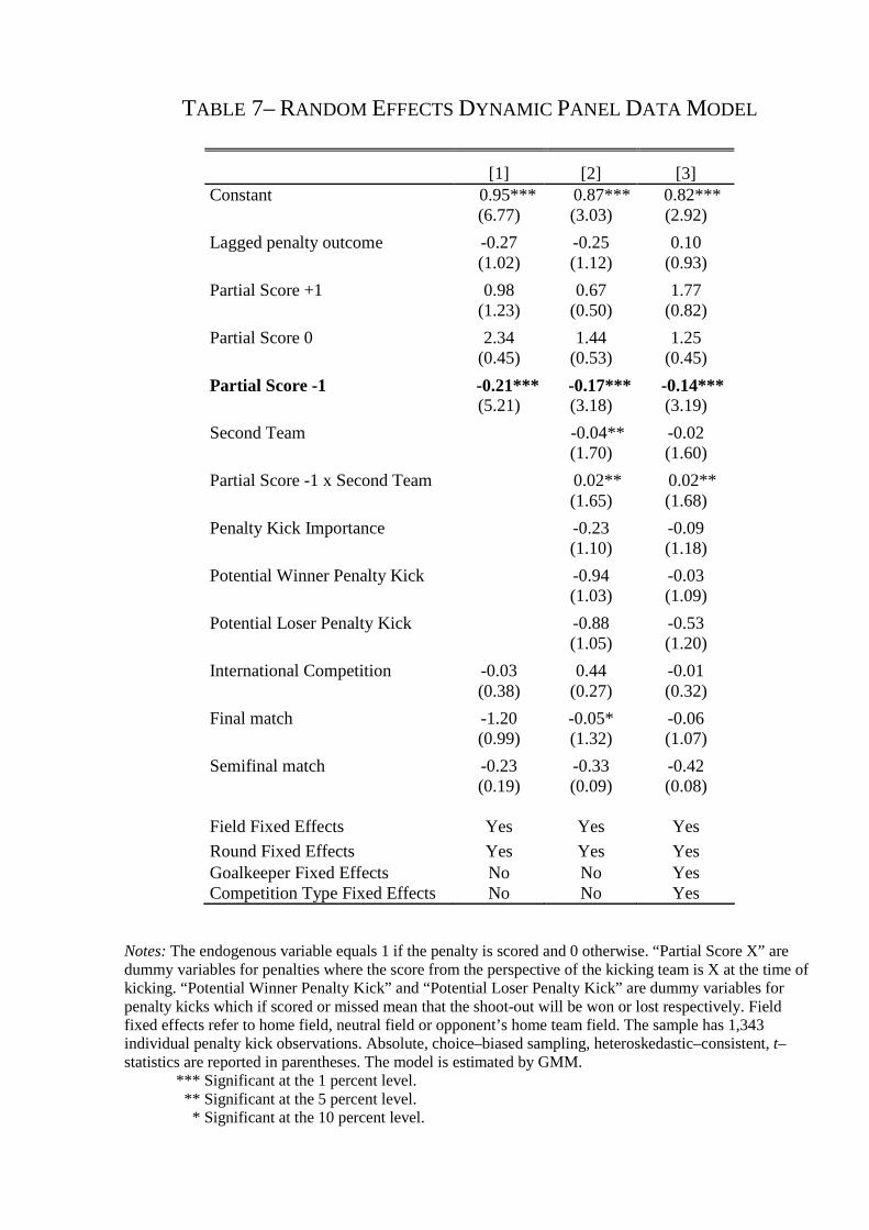
TABLE 7– RANDOM EFFECTS DYNAMIC PANEL DATA MODEL

[1] [2] [3] Constant 0.95*** 0.87*** 0.82*** (6.77) (3.03) (2.92)

Lagged penalty outcome -0.27 -0.25 0.10 (1.02) (1.12) (0.93)

Partial Score +1 0.98 0.67 1.77 (1.23) (0.50) (0.82)

Partial Score 0 2.34 1.44 1.25 (0.45) (0.53) (0.45)

Partial Score -1 -0.21*** -0.17*** -0.14*** (5.21) (3.18) (3.19)

Second Team -0.04** -0.02 (1.70) (1.60)

Partial Score -1 x Second Team 0.02** 0.02** (1.65) (1.68)

Penalty Kick Importance -0.23 -0.09 (1.10) (1.18)

Potential Winner Penalty Kick -0.94 -0.03 (1.03) (1.09)

Potential Loser Penalty Kick -0.88 -0.53 (1.05) (1.20)

International Competition -0.03 0.44 -0.01 (0.38) (0.27) (0.32)

Final match -1.20 -0.05* -0.06 (0.99) (1.32) (1.07)

Semifinal match -0.23 -0.33 -0.42 (0.19) (0.09) (0.08) Field Fixed Effects Yes Yes Yes

Round Fixed Effects Yes Yes Yes Goalkeeper Fixed Effects No No Yes Competition Type Fixed Effects No No Yes

Notes: The endogenous variable equals 1 if the penalty is scored and 0 otherwise. “Partial Score X” are dummy variables for penalties where the score from the perspective of the kicking team is X at the time of kicking. “Potential Winner Penalty Kick” and “Potential Loser Penalty Kick” are dummy variables for penalty kicks which if scored or missed mean that the shoot-out will be won or lost respectively. Field fixed effects refer to home field, neutral field or opponent’s home team field. The sample has 1,343 individual penalty kick observations. Absolute, choice–biased sampling, heteroskedastic–consistent, t–statistics are reported in parentheses. The model is estimated by GMM. *** Significant at the 1 percent level.

** Significant at the 5 percent level. * Significant at the 10 percent level.

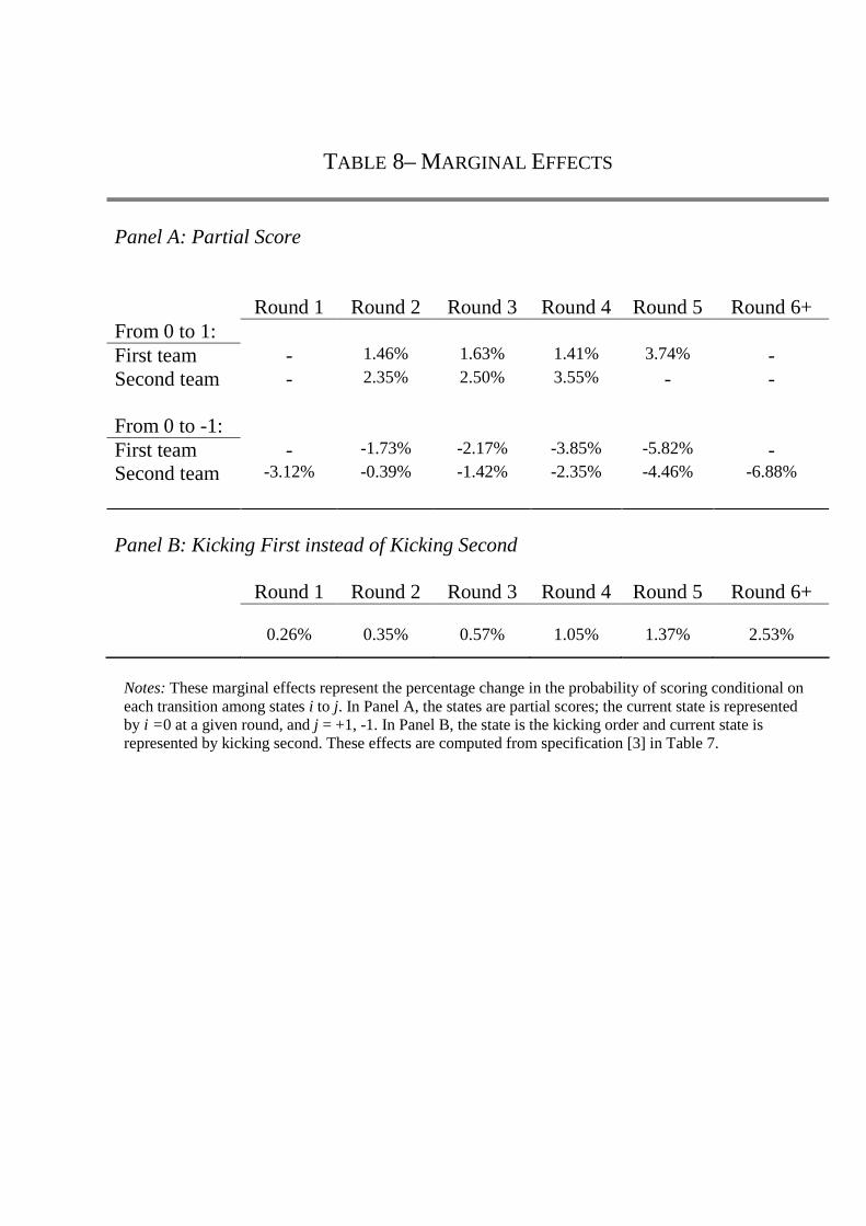
TABLE 8– MARGINAL EFFECTS

Panel A: Partial Score

Round 1

Round 2

Round 3

Round 4

Round 5

Round 6+

From 0 to 1: First team - 1.46% 1.63% 1.41% 3.74% - Second team - 2.35% 2.50% 3.55% - - From 0 to -1: First team - -1.73% -2.17% -3.85% -5.82% - Second team -3.12% -0.39% -1.42% -2.35% -4.46% -6.88%

Panel B: Kicking First instead of Kicking Second

Round 1 Round 2 Round 3 Round 4 Round 5 Round 6+

0.26%

0.35%

0.57%

1.05%

1.37%

2.53%

Notes: These marginal effects represent the percentage change in the probability of scoring conditional on each transition among states i to j. In Panel A, the states are partial scores; the current state is represented by i =0 at a given round, and j = +1, -1. In Panel B, the state is the kicking order and current state is represented by kicking second. These effects are computed from specification [3] in Table 7.

0.605

0.395

0.0

0.2

0.4

0.6

First Team Second Team

FIGURE 1. WINNING FREQUENCIES IN AGGREGATE DATA

0.79 0.820.77 0.74 0.740.72

0.77

0.640.68 0.67

0.0

0.2

0.4

0.6

0.8

1.0

1 2 3 4 5

Round

First Team Second Team

FIGURE 2A. SCORING PROBABILITIES PER ROUND

0.20

0.27

0.350.40

0.46

0.13

0.200.23

0.27 0.27

0.0

0.2

0.4

1 2 3 4 5

Round

First Team Second Team

FIGURE 2B. FREQUENCY WITH WHICH A TEAM LEADS IN THE SCORE AT THE END OF A ROUND

Notes: If before both teams have taken five penalty kicks, one has score more goals than the other could possibly score even if it were to complete its five kicks, no more kicks are taken. The percentage of times in which a team is leading in the score at the end of a round in Figure 2B includes these cases, that is, cases in which the shoot-out already ended before this round, whereas in Figure 2A the scoring rate is only computed for the teams that are observed to kick in the corresponding round.

WEB APPENDICESfor

�Psychological Pressure in CompetitiveEnvironments: Evidence from a Randomized

Natural Experiment�

September 2009

Table of Contents

Appendix A. Dynamic Panel Data Analysis with Lagged Endogenous Variables

Appendix B. A Theoretical Framework

1

APPENDIX A. Dynamic Panel Data Analysis with Lagged Endogenous

Variables.

As is well known, in the presence of lagged endogenous variables in linear models

with additive e¤ects the standard response is to consider instrumental-variables esti-

mates which exploit the lack of correlation between lagged values of the variables and

future errors in �rst di¤erences. In non-linear models, however, very few results are

available.1 In this appendix we describe the Manuel Arellano and Raquel Carrasco

(2003) model and how it is applied to the setting we study. We also report the results

of the multinomial logit analysis applied to the penalty shoot-outs for which we have

data on �goals,��misses�and �saves.�

The basic idea of the Arellano-Carrasco model is to de�ne conditional probabilities

for every possible sequence of realizations of the state variables. Then, the estimator

computes the probability of a given outcome along every possible path of past realiza-

tions of the endogenous regressors. The panel data structure allows the identi�cation

of the e¤ect of individual unobserved heterogeneity since outcomes can be di¤erent

even when teams share the same history of realizations of the state variables.

Consider two discrete outcomes (score, no score) denoted yit = f1; 0g. The proba-bility of each of them depends on the speci�c sequence of past outcomes and the state

of the shoot-out tournament. Since outcomes can be di¤erent, di¤erent experiences

change the information set and the expected realizations of future outcomes. To be

more speci�c, the probability of a given outcome may depend on certain intrinsic

characteristics of the teams involved in the shoot-out, as well as on their expectation

on the realization of the �nal outcome. This can be written as follows:

yit = 1��zit + E

��i j wti

�+ "it � 0

;

"it j wti � N�0; �2t

�;

where zit includes the set of time�invariant characteristics of the teams and the shoot-

out, xit; plus the state of the shoot-out and the previous outcomes yi(t�1). Denote

1For �xed e¤ects the few available methods are case-speci�c (logit and Poisson) and, in practice,lead to estimators that do not converge at the usual

pn-rate. In the case of random e¤ects, the

main di¢ culty is the so-called initial conditions problem: if one begins to observe subjects afterthe �process� in question is already in progress, it is necessary to isolate the e¤ect of the �rstlagged dependent variable from the individual-speci�c e¤ect and the distribution of the explanatoryvariables prior to the sample.

2

by wti = fwi1; : : : ; witg the history represented by a sequence of realizations wit =�xit; yi(t�1)

, and by �i an individual e¤ect (future outcome realization for team

i) whose forecast is revised each period t as the information summarized by the

history wti accumulates.2 The conditional distribution of the sequence of expectations

E (�i j wti) is left unrestricted, and hence the process of updating expectations asinformation accumulates is not explicitly modeled. This is the only aspect that makes

the model semi�parametric. Given the history of past outcomes, since errors are

normally distributed, the conditional probability of yit = 1 at time t for any given

history wti is:

Pr�yit = 1 j wti

�= �

��zit + E (�i j wti)

�t

�:

Since the model has discrete support, any individual history can be summarized

by a cluster of nodes j = 1; : : : ; J representing the sequence of realizations for each

vector of characteristics. Thus, the conditional probability can be rewritten as:

pjt = Pr�yit = 1 j wti = �tj

�� ht

�wti = �

tj

�; j = 1; : : : ; J:

The estimation relies on an intuitive idea. In order to remove the unobserved

individual e¤ect, we account for the proportion of teams with identical characteristics

and history up to time t that realize a given outcome at time t. We then repeat this

procedure for every cluster of combinations of demographics and histories in our data.

For each cluster we compute the percentage of times that outcome yit = 1 occurs.

This provides a simple estimate of the unrestricted probability pjt for each possible

history in the sample. Then, by taking �rst di¤erences of the inverse of the equation

above we get:

�t��1 �ht �wti��� �t�1��1 �ht�1 �wt�1i

��� �

�xit � xi(t�1)

�= �it;

and, by the law of iterated expectations, we have:

E��it j wt�1i

�= E

�E��i j wti

�� E

��i j wt�1i

���wt�1i

�= 0:

This conditional moment condition serves as the basis of the GMM estimation of

parameters � and �t (subject to the normalization restriction that �1 = 1). Arellano

2The speci�cation of Arellano and Carrasco (2003) is more general in the sense that it alsoincludes a time-varying component, t, common to all individuals. In our case all �demographic�variables are time�invariant.

3

and Carrasco (2003) show that there is no e¢ ciency loss in estimating these parame-

ters by a two�step GMM method where in the �rst step the conditional probabilities

pjt are replaced by unrestricted estimates pjt, which in our case are the proportion of

teams with given characteristics and a given history. Then:

ht�wti�=

JXj=1

1�wti = �

tj

� pjt;

can be used to de�ne the sample orthogonality conditions of Arellano�Carrasco�s

GMM estimator:3

1

N

NXi=1

dit

n�t�

�1hht�wti�i� �t�1��1

hht�1

�wt�1i

�i� �

�xit � xi(t�1)

�o= 0; t = 2; : : : ; T;

where dit is a vector containing the indicators 1�wti = �

tj

for j = 1; : : : ; J .

With respect to the magnitude of the e¤ects, the marginal e¤ects associated with

the transition among di¤erent states can be computed as follows. Arellano and Car-

rasco (2003) show that the probability of a given outcome when we compare two

states zit = z0 and zit = z1 changes by the proportion:

4t =1

N

NXi=1

n����1t �

�z1 � zit

�+ ��1

hht�wti�i�

� ����1t �

�z0 � zit

�+ ��1

hht�wti�i�o

:

Since this proportion depends on the history of past !ti, these marginal e¤ects are

di¤erent for each partial score in the sample, and for each team.

Finally, a reason why the Arellano-Carrasco is preferred in our setting is that al-

ternative �xed-e¤ects approaches such as Bo Honoré and Arthur Lewbel (2002) and

Honoré and Ekaterini Kyriazidou (2000) are far more demanding in terms of data. In

particular, they require the exogenous regressors to vary over time, something that

does not occur in our data. Honoré and Kyriazidou (2000) include one lagged depen-

dent variable but require that the remaining explanatory variables should be strictly

exogenous, thus excluding the possibility of a lagged dependent regressor. Further,

their estimator does not converge at the usualpn�rate. Honoré and Lewbel (2002)

3We use the orthogonal deviations suggested by Arellano and Olympia Bover (1995) instead of�rst di¤erences among past values of the state variables.

4

allow for additional predetermined variables but at the cost of requiring a contin-

uous, strictly exogenous, explanatory variable that is independent of the individual

e¤ects. See Ivan Fernandez-Val (2009) for a characterization of the bias of �xed e¤ect

estimators in non-linear panel data models.

Finally, as indicated in the main text of the article, for a subset of all the penalty

shoot-outs in the sample we have detailed information on whether the no-goals are

due to �saves� by the goalkeeper or �misses� by the kicker. Table A1 reports the

results of a multinomial logit speci�cation with goals, misses and saves using these

data.

[Table A1 here]

Panel A reports the raw data in scoring, misses and saving rates for the �rst and

second team. We �nd that both teams have basically the same proportion of saves,

and hence that the di¤erence in scoring rates between the �rst and the second team

basically corresponds to their di¤erence in misses.

In Panel B we report the results of di¤erent regression speci�cations. We �nd

that the coe¢ cient on �Partial score -1� is positive and highly signi�cant (beyond

the 1 percent level) for misses, but insigni�cant for saves in all the speci�cations.

This means that lagging in the score predicts more misses by the kicker but no more

saves by the goalkeeper. The interaction with the �Second team�variable is negative

and signi�cant, which means that when the partial score is -1 the �rst kicking team is

more likely to miss. This, as in Table 7, is likely the result of being in an objectively

worse situation than the second team (it has had the same number of chances of

scoring, whereas, at every kick, the second team has always had one less chance). No

variable except the constant term is signi�cant for saves. The variable �Penalty Kick

Importance,� although not signi�cant at the conventional signi�cance levels, has a

fairly high t-statistic for misses.

We take these results as consistent with the idea that the decrease in the scoring

rate for the second team, which is the one more likely to be behind in the partial

score, can be mainly attributed to an increase in misses by the kicker rather than to

an increase in saves by the goalkeeper of the opposing team.

5

REFERENCES

Arellano, Manuel, and Olympia Bover. 1995. �Another Look at the Instru-

mental Variable Estimation of Error�Components Models.�Journal of Econometrics,

68(1): 29�51.

Arellano, Manuel, and Raquel Carrasco. 2003. �Binary Choice Panel Data

Models with Predetermined Variables.�Journal of Econometrics, 115(1): 125�157.

Fernandez-Val, Ivan. 2009. �Fixed E¤ects Estimation of Structural Parameters

and Marginal E¤ects in Panel Probit Models.�Journal of Econometrics, 150(1): 71�

85.

Honoré, Bo, and Arthur Lewbel. 2002. �Semiparametric Binary Choice

Panel Data Models without Strictly Exogenous Regressors.� Econometrica, 70(5):

2053�2063.

Honoré, Bo, and Ekaterini Kyriazidou. 2000. �Panel Data Discrete Choice

Models with Lagged Dependent Variables.�Econometrica, 68(4): 839�874.

6

APPENDIX B. A Theoretical Framework

In this appendix we study a simple model that is consistent with the empirical

evidence, always predicts a �rst-mover advantage, and relies on a reference point

associated with the partial score (score at the time of kicking). After the presentation

of the model, various extensions are discussed.

Let (s; r) , with s 2 Z, r � 1 , denote the score at the end of a round r. The

score measures the di¤erence in goals between the team that kicks �rst F and the

one that kicks second D. A round involves one penalty kick for F and one for D.

The total number of rounds is n. The partial score for a team � 2 fF;Dg in roundr is the di¤erence between the goals scored by � and those scored by the opponent,

immediately before team � is about to take its penalty kick in round r. That is, for

team F the partial score at r is (s; r � 1), while, for team D; it is (�s � x; r � 1);where x = 1 if F scores in round r and x = 0 otherwise. In what follows we will use

the terms team and player indistinctly.

Denote by p 2 [0; 1] the probability of player � scoring a goal when the partialscore is tied or positive for him, and by q 2 [0; 1] the probability of player � scoring agoal when he is behind in the partial score by at least one goal. Under psychological

pressure p > q, while under no psychological pressure p = q.

For any given (s; r) with r < n there are exactly four possible outcomes at the

end of round r: (i) both players score a goal, (ii) the �rst scores and the second fails,

(iii) the �rst fails and the second scores, and (iv) both fail. The probability vectors

associated to these outcomes depend on (s; r). There are three possible cases:

1. If s = 0, then (p � q; p(1� q); (1� p)p; (1� p)2);

2. If s > 0, then (p � q; p(1� q); (1� p)q; (1� p)(1� q));

3. If s < 0, then (q � p; q(1� p); (1� q)p; (1� q)(1� p)).

To simplify notation we write a = p � q, b = p(1� q), c = (1� p)p, d = (1� p)2,e = (1 � p)q, and f = (1 � p)(1 � q). The above de�nes a Markov chain. Since weare interested in rank-order tournaments, we need to re�ne the notion of maximum

and minimum scores. If n is even, the maximum and minimum scores are n2+ 1 and

�(n2+1), while if n is odd the maximum and minimum scores are n+1

2and�(n+1

2). The

7

state space is formed by all possible scores S = fsmax; smax�1; : : : ;�1; 0; 1; : : : ; smin�1; sming with smax and smin de�ned as above. Typical elements of S are denoted bys; t or s0; s1; : : : ; sn. The transition matrix P follows from the single-step transition

probabilities pst:

p00 = a+ d; p01 = b; p0;�1 = c

s 2 fsmin; smaxg; pss = 1

s 2 S n f0; smin; smaxg; pss = a+ f

s 2 S n f0; smin; smaxg; ps;s+1 = p�s;�s�1 = b

s 2 S n f0; smin; smaxg; ps;s�1 = p�s;�s+1 = e

and pst = 0 otherwise. The initial distribution � puts all the probability mass in

state 0. Denote by T (n; P ) the n-round sequential tournament between F andD with

transition matrix P . Denote by p(n)st the (s; t) entry in the n-th power of the transition

matrix P . Since the Markov chain is stationary, p(n)st represents the probability of

reaching state t starting from state s in n rounds.

The probability that team F wins the n-round sequential tournament T (n; P ) is:

W (F; n) =s=smaxXs=1

P (s; n);

with P (s; n) denoting the probability of a �nal score s. To calculate P (s; n) we have

to correct for the probability of reaching a �nal state in some previous round. A �nal

state is a pair (s; r) where there is no possibility of turning around the sign of the

score s in the remaining time n� r. Then we have that:

P (1; n) = p(n)01 � p

(n�1)02 p21;

P (smax; n) = p(n+1�smax)0;smax�1 psmax�1;smax + p

(n+1�smax)0smax ;

and for 1 < s < smax :

P (s; n) = p(n+1�s)0;s�1 ps�1;s + p

(n+1�s)0s � p(n�s)0;s+1ps+1;s:

In principle, these probabilities can be obtained using standard matrix algebra. The

probability of team D winning at the end of the n-round contestW (D;n) is obtained

analogously.

8

Denote by W (�; r) the probability that � is either ahead of its opponent at the

end of round r � n or has already won the tournament by then. We are now readyto derive convenient formulations for W (F; r) and W (D; r).

Proposition 1. Let T (n; P ) be an n-round sequential tournament. Then, for

every r � n, W (F; r) = bb+c(1� p(r)00 ) and W (D; r) = c

b+c(1� p(r)00 ).

Proof: Take any path ending in state s > 0 in round r, and denote it by

s0s1 � � � sr�1sr with s0 = 0 and sr = s. The probability measure of such path is

ps0s1 � � � psr�1;sr . We distinguish two cases:(1) First, the path s0s1 � � � sr�1sr does not reach a �nal state s0 in some previous

round h < r. We construct a unique symmetric path to the original one, ending in

state �s. If sr�1 = 0, stop. Otherwise, proceed backwards until reaching a k, 0 � k �r�1; such that sk = 0. Clearly, such a k exists. Then, for every l � k write s0l = �sl,and write s0l = sl otherwise. It is immediate that the constructed path s

00s01 � � � s0r�1s0r

starts with s00 = 0, ends in s0r = �s, does not go through any �nal state, and hasan associated probability measure of ps00s01 � � � ps0r�1;s0r , where ps0l;s0l+1 = psl;sl+1 for everyl 6= k, while b = psk;sk+1 � ps0k;s0k+1 = c. That is, the di¤erence in the probability

measures between the two paths is (b� c)ps0s1 � � � psk�1;skpsk+1;sk+2 � � � psr�1;sr .(2) Second, the path s0s1 � � � sr�1sr does reach a �nal state s0 in a previous round

h < r. First, we modify the path s0s1 � � � sr�1sr to correct for the sub-path fol-lowing the �nal state s0 by writing sh = sh+1 = � � � = sr�1 = sr = s0, with asso-

ciated probability measure �psl;sl+1 = psl;sl+1 whenever sl � h � 1, and �psl;sl+1 = 1

whenever sl > h � 1. Second, we apply the same argument as before to the mod-i�ed path to show that there exists a unique symmetric path ending in �nal state

�s0, and where the di¤erence in the probability measures between the two paths is(b� c)�ps0s1 � � � �psk�1;sk �psk+1;sk+2 � � � �psr�1;sr .Consequently, it is immediate that there exists a probability mass (r) such that

W (A; r) = b (r) and W (B; r) = c (r). Note that by de�nition of �nal states,

p(r)00 does not reach any �nal state in some previous round h � r. Now since

W (A; r) + W (B; r) + p(r)00 = 1, it follows that (r) = 1

b+c(1 � p

(r)00 ), and hence

W (A; r) = bb+c(1� p(r)00 ) and W (B; r) = c

b+c(1� p(r)00 ).�

Since under no psychological pressure p = q implies b = c, it directly follows from

9

Proposition 1 that W (F; n) = W (D;n). On the other hand, under psychological

pressure, that is when p > q, we have that b > c, and hence Proposition 1 implies

that W (F; n) > W (D;n). We summarize the above in the following corollary:

Corollary. Let T (n; P ) be an n-round sequential tournament. Then, for every

p; q 2 [0; 1], and for every r � n, if p = q then W (F; r) = W (D; r), and when p > q,W (F; r) > W (D; r).

The main merit of the model is that it only takes two parameters to predict a

greater probability of the �rst team winning. This simplicity involves strong assump-

tions and is not without limitations which further generalizations of the model may

address. For instance, in order to capture the possibility of order-dependent technolo-

gies, it is possible to consider the di¤erence p� q to be team-speci�c or alternativelya four-parameter model (p�; q�), � = F;D. For example, a partial score of 0 is better

news for the second team than for the �rst team, and this may have an impact on

performance. These considerations will readily enrich the model and can be easily

incorporated. In the latter case, for instance, it can be shown that the advantage of

one team over the other depends on the parameter range of the (p�; q�) values, and

that it is possible to �nd parameter values where both the �rst team has an advantage

over the second and vice versa. Examples are available upon request.

Finally, the assumption that all team players use the same (p; q) technology can

be generalized to introduce heterogeneity in player quality: f(ph; qh)gh2Q, where Qis the set of players of a team ordered by quality. This opens up the possibility of

investigating the strategic placement of players throughout the tournament, a decision

that is taken before the toss out. We have studied this extension by having the two

teams with (the same) two types of players di¤ering in their (p; q) technology compete

in a tournament with just 2 rounds. We have found that, even in this simple case,

it is possible to �nd parameters within an empirically sensible range of values that

make each of the 4 possible combinations of the players a Nash equilibrium. That

is, in theory, any combination could be optimal. This means that without precise

information regarding the technologies of each player, it is not possible to have a

sharp, testable implication on the strategic allocation of players.

For instance, consider the two teams F and D competing in a tournament with

only 2 rounds. Each team has two players: H and L. Player H plays with technology

10

(ph; qh), ph � qh, and player L plays with (pl; ql), pl � ql, where ph > pl. Assume thatone of the players is vulnerable to psychological pressure, and hence plays with pi > qi,

and the other player is not vulnerable, and hence he plays with pj = qj; i; j 2 fH;Lg,i 6= j. Denote by (��; �) the order in which team � 2 fF;Dg places the players Hand L in the 2 rounds. For example, (�F ; F ) = (L;H) means that the �rst team

F places player L in round 1 and player H in round 2. Let W (�; (�F ; F ); (�D; D))

denote the probability of winning for team � when the �rst team chooses the order

(�F ; F ) and the second team chooses the order (�D; D). It is immediate to show

that:

W (F; (H;L); (H;L))�W (F; (L;H); (H;L)) = (ph � pl)(1� ql)(ph � qh) (1)

W (F; (H;L); (L;H))�W (F; (L;H); (L;H)) = (ph � pl)(1� qh)(pl � ql) (2)

W (D; (H;L); (H;L))�W (D; (H;L); (L;H)) = (ph � pl)(1� ph)(pl � ql)

+ ph(1� pl)(qhpl � qlph) (3)

W (D; (L;H); (H;L))�W (D; (L;H); (L;H)) = (ph � pl)(1� pl)(ph � qh)

+ pl(1� ph)(qhpl � qlph) (4)

It then follows that:

(i). When player L is the vulnerable player, and hence ph = qh > pl > ql, equation

(1) is equal to 0, and equations (2), (3), and (4) are all strictly positive. Hence, there

are two pure strategy Nash equilibria: ((H;L); (H;L)) and ((L;H); (H;L)).

(ii). When player H is the vulnerable player, and hence ph > qh and ph >

pl = ql, equation (1) is strictly positive, equation (2) is equal to 0, equation (3) is

strictly negative, and the sign of equation (4) is equal to the sign of A = (ph � pl +phpl(pl � 1)).4 Consequently, ((H;L); (L;H)) is a pure strategy Nash equilibrium,

and ((L;H); (L;H)) will be another pure strategy Nash equilibrium when A � 0.

Therefore, even in this simple version of a penalty shootout, the four possible

placements of the players could be a pure strategy Nash equilibrium. Hence, without

4Empirically plausible parameters for each potential case can be readily found. For example,A < 0 when ph = 0:8 and pl = 0:7; A > 0 when ph = 0:85 and pl = 0:65; and A = 0 whenph = 0:65=0:7725 ' 0:841 and pl = 0:65.

11

precise information on who is the vulnerable player (and when H is the vulnerable

player, on the speci�c values of ph and pl) no testable prediction on the strategic

allocation of players obtains.

12

TABLE A.1– DETERMINANTS OF MISSES AND SAVES

Panel A: Proportions of Penalties Scored, Saved and Missed No Scored

N

(penalties) Scored Saved Missed First team 234 75.6% 17.1% 7.3% Second team 220 68.6% 16.8% 14.6% Difference: -7.0% -0.3% +7.3%

Panel B: Panel Data Analysis for Misses and Saves

Misses

Saves

[1]

[2]

[3]

[4]

Constant -1.57*** -1.70*** -0.98** -0.67** (3.01) (2.57) (2.15) (2.23)

Partial Score -1 0.09*** 0.17*** -0.17 -0.12 (2.65) (2.85) (0.44) (0.36)

Partial Score 0 0.46 0.33 0.15 0.06 (0.33) (0.12) (0.27) (0.16) Partial Score +1

0.09

0.17 0.88 -0.47

(0.93) (0.77) (0.38) (0.36) Second Team

0.27

0.15

0.10 -0.22

(0.67) (0.49) (0.55) (0.68) Partial Score -1 x Second Team

-0.009**

-0.005**

0.006 0.015

(2.06) (1.90) (1.03) (0.70)

Penalty Kick Importance

1.05

(1.12)

1.17

(1.10)

0.44

(0.88)

0.83

(0.47)

Round Fixed Effect

No

Yes

No

Yes

Goalkeeper Fixed Effect No Yes No Yes

N 454 454 454 454

Notes: Misses by kicker are penalty kicks shot to the upright posts, the horizontal crossbar or outside the goal. Saves are penalty kicks stopped by the goalkeeper. All the specifications include Field, Competition and Match type fixed effects, as well as controls for “Potential Winner” and “Potential Loser” penalty kicks. Absolute, choice–biased sampling, heteroskedastic-consistent, t–statistics are reported in parentheses.

*** Significant at the 1 percent level. ** Significant at the 5 percent level.