joint models for longitudinal and survival data - … · joint models for longitudinal and survival...
TRANSCRIPT

Joint Models for Longitudinal and Survival Data
Dimitris RizopoulosDepartment of Biostatistics, Erasmus University Medical Center
Erasmus Summer Program 2018
August 13-17, 2018

Contents
I Introduction 1
1.1 Motivating Longitudinal Studies . . . . . . . . . . . . . . . . . . . . . . . . . . 2
1.2 Research Questions . . . . . . . . . . . . . . . . . . . . . . . . . . . . . . . 10
1.3 Recent Developments . . . . . . . . . . . . . . . . . . . . . . . . . . . . . . 13
1.4 Joint Models . . . . . . . . . . . . . . . . . . . . . . . . . . . . . . . . . . 15
II Linear Mixed-Effects Models 18
2.1 Features of Longitudinal Data . . . . . . . . . . . . . . . . . . . . . . . . . . . 19
2.2 The Linear Mixed Model . . . . . . . . . . . . . . . . . . . . . . . . . . . . . 21
Joint Models for Longitudinal and Survival Data: August 13-17, 2018, Rotterdam ii

2.3 Mixed Models with Correlated Errors . . . . . . . . . . . . . . . . . . . . . . . . 32
2.4 Mixed-Effects Models in R . . . . . . . . . . . . . . . . . . . . . . . . . . . . 36
2.5 Missing Data in Longitudinal Studies . . . . . . . . . . . . . . . . . . . . . . . . 42
2.6 Missing Data Mechanisms . . . . . . . . . . . . . . . . . . . . . . . . . . . . 46
III Relative Risk Models 55
3.1 Features of Survival Data . . . . . . . . . . . . . . . . . . . . . . . . . . . . . 56
3.2 Basic functions in Survival Analysis . . . . . . . . . . . . . . . . . . . . . . . . . 59
3.3 Relative Risk Models . . . . . . . . . . . . . . . . . . . . . . . . . . . . . . . 62
3.4 Relative Risk Models in R . . . . . . . . . . . . . . . . . . . . . . . . . . . . . 67
3.5 Time Dependent Covariates . . . . . . . . . . . . . . . . . . . . . . . . . . . . 69
Joint Models for Longitudinal and Survival Data: August 13-17, 2018, Rotterdam iii

3.6 Extended Cox Model . . . . . . . . . . . . . . . . . . . . . . . . . . . . . . . 74
IV The Basic Joint Model 80
4.1 Joint Modeling Framework . . . . . . . . . . . . . . . . . . . . . . . . . . . . 81
4.2 Estimation . . . . . . . . . . . . . . . . . . . . . . . . . . . . . . . . . . . 93
4.3 Bayesian Estimation . . . . . . . . . . . . . . . . . . . . . . . . . . . . . . . 99
4.4 A Comparison with the TD Cox . . . . . . . . . . . . . . . . . . . . . . . . . . 103
4.5 Joint Models in R . . . . . . . . . . . . . . . . . . . . . . . . . . . . . . . . 106
4.6 Connection with Missing Data . . . . . . . . . . . . . . . . . . . . . . . . . . . 112
Joint Models for Longitudinal and Survival Data: August 13-17, 2018, Rotterdam iv

V Extensions of Joint Models 122
5.1 Parameterizations . . . . . . . . . . . . . . . . . . . . . . . . . . . . . . . . 123
5.2 Latent Class Joint Models . . . . . . . . . . . . . . . . . . . . . . . . . . . . 143
5.3 Multiple Longitudinal Markers . . . . . . . . . . . . . . . . . . . . . . . . . . . 151
5.4 Multiple Failure Times . . . . . . . . . . . . . . . . . . . . . . . . . . . . . . 158
5.5 Time-Dependent AFT Models . . . . . . . . . . . . . . . . . . . . . . . . . . . 169
5.6 Extensions & Parameterizations . . . . . . . . . . . . . . . . . . . . . . . . . . 174
VI Dynamic Predictions, Discrimination & Calibration 178
6.1 Survival Probabilities: Definitions . . . . . . . . . . . . . . . . . . . . . . . . . 179
6.2 Survival Probabilities: Estimation . . . . . . . . . . . . . . . . . . . . . . . . . 183
Joint Models for Longitudinal and Survival Data: August 13-17, 2018, Rotterdam v

6.3 Dynamic Predictions using Landmarking . . . . . . . . . . . . . . . . . . . . . . 194
6.4 Longitudinal Responses: Definitions . . . . . . . . . . . . . . . . . . . . . . . . 198
6.5 Importance of the Parameterization . . . . . . . . . . . . . . . . . . . . . . . . 206
6.6 Marker Discrimination: Definitions . . . . . . . . . . . . . . . . . . . . . . . . . 214
6.7 Marker Discrimination: Estimation . . . . . . . . . . . . . . . . . . . . . . . . . 221
6.8 Model Discrimination . . . . . . . . . . . . . . . . . . . . . . . . . . . . . . . 226
6.9 Calibration . . . . . . . . . . . . . . . . . . . . . . . . . . . . . . . . . . . 234
6.10 Landmarking vs JM: An Example . . . . . . . . . . . . . . . . . . . . . . . . . 240
6.11 Validation . . . . . . . . . . . . . . . . . . . . . . . . . . . . . . . . . . . 245
Joint Models for Longitudinal and Survival Data: August 13-17, 2018, Rotterdam vi

VII Closing 246
7.1 Concluding Remarks . . . . . . . . . . . . . . . . . . . . . . . . . . . . . . . 247
7.2 Additional References . . . . . . . . . . . . . . . . . . . . . . . . . . . . . . 251
7.3 Medical Papers with Joint Modeling . . . . . . . . . . . . . . . . . . . . . . . . 259
VIII Practicals 261
8.1 Practical 1: A Simple Joint Model . . . . . . . . . . . . . . . . . . . . . . . . . 262
8.2 Practical 2: Challenging jointModel() . . . . . . . . . . . . . . . . . . . . . . 271
8.3 Practical 3: Using derivForm . . . . . . . . . . . . . . . . . . . . . . . . . . . 276
8.4 Practical 4: Dynamic Predictions . . . . . . . . . . . . . . . . . . . . . . . . . 285
Joint Models for Longitudinal and Survival Data: August 13-17, 2018, Rotterdam vii

What is this Course About
• Often in follow-up studies different types of outcomes are collected
• Explicit outcomes
multiple longitudinal responses (e.g., markers, blood values)
time-to-event(s) of particular interest (e.g., death, relapse)
• Implicit outcomes
missing data (e.g., dropout, intermittent missingness)
random visit times
Joint Models for Longitudinal and Survival Data: August 13-17, 2018, Rotterdam viii
What is this Course About (cont’d)
• Methods for the separate analysis of such outcomes are well established in theliterature
• Survival data:
Cox model, accelerated failure time models, . . .
• Longitudinal data
mixed effects models, GEE, marginal models, . . .
Joint Models for Longitudinal and Survival Data: August 13-17, 2018, Rotterdam ix
What is this Course About (cont’d)
Purpose of this course is to present the state of the art in
Joint Modeling Techniquesfor Longitudinal and Survival Data
Joint Models for Longitudinal and Survival Data: August 13-17, 2018, Rotterdam x

Learning Objectives
• Goals: After this course participants will be able to
identify settings in which a joint modeling approach is required,
construct and fit an appropriate joint model, and
correctly interpret the obtained results
• The course will be explanatory rather than mathematically rigorous
emphasis is given on sufficient detail in order for participants to obtain a clearview on the different joint modeling approaches, and how they should be used inpractice
Joint Models for Longitudinal and Survival Data: August 13-17, 2018, Rotterdam xi
Agenda
• Part I: Introduction
Data sets that we will use throughout the course
Categorization of possible research questions
• Part II: (brief) Review of Linear Mixed Models
Features of repeated measurements data
Linear mixed models
Missing data in longitudinal studies
Joint Models for Longitudinal and Survival Data: August 13-17, 2018, Rotterdam xii

Agenda (cont’d)
• Part III: (brief) Review of Relative Risk Models
Features of survival data
Relative risk models
Time-dependent covariates
• Part IV: The Basic Joint Model
Definition
Estimation & Inference
Connection with the missing data framework
Joint Models for Longitudinal and Survival Data: August 13-17, 2018, Rotterdam xiii

Agenda (cont’d)
• Part V: Extensions of the Basic Joint Model
Parameterizations
Latent class joint models
Other extensions for the longitudinal and survival submodels (briefly)
• Part VI: Dynamic Predictions
Individualized predictions for the survival and longitudinal outcomes
Effect of the parameterization
Accuracy measures (if we have the time)
Joint Models for Longitudinal and Survival Data: August 13-17, 2018, Rotterdam xiv

Structure of the Course & Material
• Lectures & short software practicals using R package JM and/or JMbayes
• Material (also available in http://www.drizopoulos.com/):
Course Notes
R code in soft format
• Within the course notes there are several examples of R code which are denoted bythe symbol ‘R> ’
Joint Models for Longitudinal and Survival Data: August 13-17, 2018, Rotterdam xv

Schedule
• 08:45 – 10:00
• Coffee break
• 10:15 – 11:45
Joint Models for Longitudinal and Survival Data: August 13-17, 2018, Rotterdam xvi
References
• Joint modeling sources∗
Rizopoulos, D. (2012). Joint Models for Longitudinal and Time-to-Event Data,with Applications in R. Boca Raton: Chapman & Hall/CRC.
Fitzmaurice, G., Davidian, M., Verbeke, G. and Molenberghs, G. (2009).Longitudinal Data Analysis. Handbooks of Modern Statistical Methods. BocaRaton: Chapman & Hall/CRC, Chapter 15.
Wu, L. (2009). Mixed Effects Models for Complex Data. Boca Raton: Chapman& Hall/CRC, Chapter 8.
Ibrahim, J., Chen, M.-H. and Sinha, D. (2001). Bayesian Survival Analysis. NewYork: Springer-Verlag, Chapter 7.
∗ extra references of papers using joint modeling available at pp. 251–258.
Joint Models for Longitudinal and Survival Data: August 13-17, 2018, Rotterdam xvii

References (cont’d)
• Useful material for package JM can be found in the web sites:
http://jmr.r-forge.r-project.org [R code used in the book]
http://www.drizopoulos.com/ → Software [additional R script files]
• Useful material for package JMbayes
a paper describing the current capabilities of the package is available on JSShttp://dx.doi.org/10.18637/jss.v072.i07
• Blog about joint modeling http://iprogn.blogspot.nl/
Joint Models for Longitudinal and Survival Data: August 13-17, 2018, Rotterdam xviii

References (cont’d)
• Other software packages capable of fitting joint models
in R: joineR (by Philipson et al.), lcmm (by Proust-Lima et al.)
in SAS: %JM macro (by Garcia-Hernandez and Rizopoulos –http://www.jm-macro.com/), %JMFit macro (by Zhang et al.)
in STATA: stjm (by Crowther)
Joint Models for Longitudinal and Survival Data: August 13-17, 2018, Rotterdam xix
References (cont’d)
• Standard texts in survival analysis
Kalbfleisch, J. and Prentice, R. (2002). The Statistical Analysis of Failure TimeData, 2nd Ed.. New York: Wiley.
Therneau, T. and Grambsch, P. (2000). Modeling Survival Data: Extending theCox Model. New York: Springer-Verlag.
Cox, D. and Oakes, D. (1984). Analysis of Survival Data. London: Chapman &Hall.
Andersen, P., Borgan, O., Gill, R. and Keiding, N. (1993). Statistical ModelsBased on Counting Processes. New York: Springer-Verlag.
Klein, J. and Moeschberger, M. (2003). Survival Analysis - Techniques forCensored and Truncated Data. New York: Springer-Verlag.
Joint Models for Longitudinal and Survival Data: August 13-17, 2018, Rotterdam xx

References (cont’d)
• Standard texts in longitudinal data analysis
Verbeke, G. and Molenberghs, G. (2000). Linear Mixed Models for LongitudinalData. New York: Springer-Verlag.
Molenberghs, G. and Verbeke, G. (2005). Models for Discrete Longitudinal Data.New York: Springer-Verlag.
Fitzmaurice, G., Laird, N., and Ware, J. (2004). Applied Longitudinal Analysis.Hoboken: Wiley.
Diggle, P., Heagerty, P., Liang, K.-Y., and Zeger, S. (2002). Analysis ofLongitudinal Data, 2nd edition. New York: Oxford University Press.
Joint Models for Longitudinal and Survival Data: August 13-17, 2018, Rotterdam xxi

Part I
Introduction
Joint Models for Longitudinal and Survival Data: August 13-17, 2018, Rotterdam 1

1.1 Motivating Longitudinal Studies
• AIDS: 467 HIV infected patients who had failed or were intolerant to zidovudinetherapy (AZT) (Abrams et al., NEJM, 1994)
• The aim of this study was to compare the efficacy and safety of two alternativeantiretroviral drugs, didanosine (ddI) and zalcitabine (ddC)
• Outcomes of interest:
time to death
randomized treatment: 230 patients ddI and 237 ddC
CD4 cell count measurements at baseline, 2, 6, 12 and 18 months
prevOI: previous opportunistic infections
Joint Models for Longitudinal and Survival Data: August 13-17, 2018, Rotterdam 2

1.1 Motivating Longitudinal Studies (cont’d)
Time (months)
CD
4 ce
ll co
unt
0
5
10
15
20
25
0 5 10 15
ddC
0 5 10 15
ddI
Joint Models for Longitudinal and Survival Data: August 13-17, 2018, Rotterdam 3

1.1 Motivating Longitudinal Studies (cont’d)
0 5 10 15 20
0.0
0.2
0.4
0.6
0.8
1.0
Kaplan−Meier Estimate
Time (months)
Sur
viva
l Pro
babi
lity
ddC
ddI
Joint Models for Longitudinal and Survival Data: August 13-17, 2018, Rotterdam 4

1.1 Motivating Longitudinal Studies (cont’d)
• Research Questions:
How strong is the association between CD4 cell count and the risk for death?
Is CD4 cell count a good biomarker?
* if treatment improves CD4 cell count, does it also improve survival?
Joint Models for Longitudinal and Survival Data: August 13-17, 2018, Rotterdam 5

1.1 Motivating Longitudinal Studies (cont’d)
• PBC: Primary Biliary Cirrhosis:
a chronic, fatal but rare liver disease
characterized by inflammatory destruction of the small bile ducts within the liver
• Data collected by Mayo Clinic from 1974 to 1984 (Murtaugh et al., Hepatology, 1994)
• Outcomes of interest:
time to death and/or time to liver transplantation
randomized treatment: 158 patients received D-penicillamine and 154 placebo
longitudinal serum bilirubin levels
Joint Models for Longitudinal and Survival Data: August 13-17, 2018, Rotterdam 6

1.1 Motivating Longitudinal Studies (cont’d)
Time (years)
log
seru
m B
iliru
bin
−10123
38
0 5 10
39 51
0 5 10
68
70 82 90
−10123
93
−10123
134 148 173 200
0 5 10
216 242
0 5 10
269
−10123
290
Joint Models for Longitudinal and Survival Data: August 13-17, 2018, Rotterdam 7

1.1 Motivating Longitudinal Studies (cont’d)
0 2 4 6 8 10 12 14
0.0
0.2
0.4
0.6
0.8
1.0
Kaplan−Meier Estimate
Time (years)
Sur
viva
l Pro
babi
lity
placebo
D−penicil
Joint Models for Longitudinal and Survival Data: August 13-17, 2018, Rotterdam 8

1.1 Motivating Longitudinal Studies (cont’d)
• Research Questions:
How strong is the association between bilirubin and the risk for death?
How the observed serum bilirubin levels could be utilized to provide predictions ofsurvival probabilities?
Can bilirubin discriminate between patients of low and high risk?
Joint Models for Longitudinal and Survival Data: August 13-17, 2018, Rotterdam 9

1.2 Research Questions
• Depending on the questions of interest, different types of statistical analysis arerequired
• We will distinguish between two general types of analysis
separate analysis per outcome
joint analysis of outcomes
• Focus on each outcome separately
does treatment affect survival?
are the average longitudinal evolutions different between males and females?
. . .
Joint Models for Longitudinal and Survival Data: August 13-17, 2018, Rotterdam 10

1.2 Research Questions (cont’d)
• Focus on multiple outcomes
Complex hypothesis testing: does treatment improve the average longitudinalprofiles in all markers?
Complex effect estimation: how strong is the association between the longitudinalevolution of CD4 cell counts and the hazard rate for death?
Association structure among outcomes:
* how the association between markers evolves over time (evolution of theassociation)
* how marker-specific evolutions are related to each other (association of theevolutions)
Joint Models for Longitudinal and Survival Data: August 13-17, 2018, Rotterdam 11
1.2 Research Questions (cont’d)
Prediction: can we improve prediction for the time to death by considering allmarkers simultaneously?
Handling implicit outcomes: focus on a single longitudinal outcome but withdropout or random visit times
Joint Models for Longitudinal and Survival Data: August 13-17, 2018, Rotterdam 12
1.3 Recent Developments
• Up to now emphasis has been
restricted or coerced to separate analysis per outcome
or given to naive types of joint analysis (e.g., last observation carried forward)
• Main reasons
lack of appropriate statistical methodology
lack of efficient computational approaches & software
Joint Models for Longitudinal and Survival Data: August 13-17, 2018, Rotterdam 13

1.3 Recent Developments (cont’d)
• However, recently there has been an explosion in the statistics and biostatisticsliterature of joint modeling approaches
• Many different approaches have been proposed that
can handle different types of outcomes
can be utilized in pragmatic computing time
can be rather flexible
most importantly: can answer the questions of interest
Joint Models for Longitudinal and Survival Data: August 13-17, 2018, Rotterdam 14

1.4 Joint Models
• Let Y1 and Y2 two outcomes of interest measured on a number of subjects for whichjoint modeling is of scientific interest
both can be measured longitudinally
one longitudinal and one survival
• We have various possible approaches to construct a joint density p(y1, y2) of Y1, Y2 Conditional models: p(y1, y2) = p(y1)p(y2 | y1)
Copulas: p(y1, y2) = cF(y1),F(y2)p(y1)p(y2)
But Random Effects Models have (more or less) prevailed
Joint Models for Longitudinal and Survival Data: August 13-17, 2018, Rotterdam 15

1.4 Joint Models (cont’d)
• Random Effects Models specify
p(y1, y2) =
∫p(y1, y2 | b) p(b) db
=
∫p(y1 | b) p(y2 | b) p(b) db
Unobserved random effects b explain the association between Y1 and Y2
Conditional Independence assumption
Y1 ⊥⊥ Y2 | b
Joint Models for Longitudinal and Survival Data: August 13-17, 2018, Rotterdam 16
1.4 Joint Models (cont’d)
• Features:
Y1 and Y2 can be of different type
* one continuous and one categorical
* one continuous and one survival
* . . .
Extensions to more than two outcomes straightforward
Specific association structure between Y1 and Y2 is assumed
Computationally intensive (especially in high dimensions)
Joint Models for Longitudinal and Survival Data: August 13-17, 2018, Rotterdam 17

Part II
Linear Mixed-Effects Models
Joint Models for Longitudinal and Survival Data: August 13-17, 2018, Rotterdam 18

2.1 Features of Longitudinal Data
• Repeated evaluations of the same outcome in each subject in time
CD4 cell count in HIV-infected patients
serum bilirubin in PBC patients
• Longitudinal studies allow to investigate
1. how treatment means differ at specific time points, e.g., at the end of the study(cross-sectional effect)
2. how treatment means or differences between means of treatments change overtime (longitudinal effect)
Joint Models for Longitudinal and Survival Data: August 13-17, 2018, Rotterdam 19
2.1 Features of Longitudinal Data (cont’d)
Measurements on the same subject are expected tobe (positively) correlated
• This implies that standard statistical tools, such as the t-test and simple linearregression that assume independent observations, are not optimal for longitudinaldata analysis.
Joint Models for Longitudinal and Survival Data: August 13-17, 2018, Rotterdam 20
2.2 The Linear Mixed Model
• The direct approach to model correlated data ⇒ multivariate regression
yi = Xiβ + εi, εi ∼ N (0, Vi),
where
yi the vector of responses for the ith subject
Xi design matrix describing structural component
Vi covariance matrix describing the correlation structure
• There are several options for modeling Vi, e.g., compound symmetry, autoregressiveprocess, exponential spatial correlation, Gaussian spatial correlation, . . .
Joint Models for Longitudinal and Survival Data: August 13-17, 2018, Rotterdam 21
2.2 The Linear Mixed Model (cont’d)
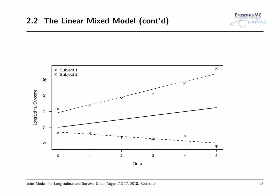
• Alternative intuitive approach: Each subject in the population has her ownsubject-specific mean response profile over time
Joint Models for Longitudinal and Survival Data: August 13-17, 2018, Rotterdam 22
2.2 The Linear Mixed Model (cont’d)
0 1 2 3 4 5
020
4060
80
Time
Long
itudi
nal O
utco
me
Subject 1
Subject 2
Joint Models for Longitudinal and Survival Data: August 13-17, 2018, Rotterdam 23

2.2 The Linear Mixed Model (cont’d)
• The evolution of each subject in time can be described by a linear model
yij = βi0 + βi1tij + εij, εij ∼ N (0, σ2),
where
yij the jth response of the ith subject
βi0 is the intercept and βi1 the slope for subject i
• Assumption: Subjects are randomly sampled from a population ⇒ subject-specificregression coefficients are also sampled from a population of regression coefficients
βi ∼ N (β,D)
Joint Models for Longitudinal and Survival Data: August 13-17, 2018, Rotterdam 24
2.2 The Linear Mixed Model (cont’d)
• We can reformulate the model as
yij = (β0 + bi0) + (β1 + bi1)tij + εij,
where
βs are known as the fixed effects
bis are known as the random effects
• In accordance for the random effects we assume
bi =
bi0bi1
∼ N (0, D)
Joint Models for Longitudinal and Survival Data: August 13-17, 2018, Rotterdam 25
2.2 The Linear Mixed Model (cont’d)
• Put in a general formyi = Xiβ + Zibi + εi,
bi ∼ N (0, D), εi ∼ N (0, σ2Ini),
with
X design matrix for the fixed effects β
Z design matrix for the random effects bi
bi ⊥⊥ εi
Joint Models for Longitudinal and Survival Data: August 13-17, 2018, Rotterdam 26

2.2 The Linear Mixed Model (cont’d)
• Interpretation:
βj denotes the change in the average yi when xj is increased by one unit
bi are interpreted in terms of how a subset of the regression parameters for the ithsubject deviates from those in the population
• Advantageous feature: population + subject-specific predictions
β describes mean response changes in the population
β + bi describes individual response trajectories
Joint Models for Longitudinal and Survival Data: August 13-17, 2018, Rotterdam 27

2.2 The Linear Mixed Model (cont’d)
• How do the random effects capture correlation:
Given the random effects, the measurements of each subject are independent(conditional independence assumption)
p(yi | bi) =ni∏j=1
p(yij | bi)
Marginally (integrating out the random effects), the measurements of each subjectare correlated
p(yi) =
∫p(yi | bi) p(bi) dbi ⇒ yi ∼ N (Xiβ, ZiDZ
⊤i + σ2Ini)
Joint Models for Longitudinal and Survival Data: August 13-17, 2018, Rotterdam 28
2.2 The Linear Mixed Model (cont’d)
• Estimation
Fixed effects: For known marginal covariance matrix Vi = ZiDZ⊤i + σ2Ini, the
fixed effects are estimated using generalized least squares
β =
(n∑i=1
X⊤i V
−1i Xi
)−1 n∑i=1
X⊤i V
−1i yi
Variance Components: The unique parameters in Vi are estimated based on eithermaximum likelihood (ML) or restricted maximum likelihood (REML)
* REML provides unbiased estimates for the variance components in smallsamples
Joint Models for Longitudinal and Survival Data: August 13-17, 2018, Rotterdam 29

2.2 The Linear Mixed Model (cont’d)
• Example: We fit a linear mixed model for the AIDS dataset assuming
different average longitudinal evolutions per treatment group (fixed part)
random intercepts & random slopes (random part)
yij = β0 + β1tij + β2ddIi × tij + bi0 + bi1tij + εij,
bi ∼ N (0, D), εij ∼ N (0, σ2)
• Note: We did not include a main effect for treatment due to randomization
Joint Models for Longitudinal and Survival Data: August 13-17, 2018, Rotterdam 30

2.2 The Linear Mixed Model (cont’d)
Value Std.Err. t-value p-value
β0 7.189 0.222 32.359 < 0.001
β1 −0.163 0.021 −7.855 < 0.001
β2 0.028 0.030 0.952 0.342
• No evidence of differences in the average longitudinal evolutions between the twotreatments
Joint Models for Longitudinal and Survival Data: August 13-17, 2018, Rotterdam 31

2.3 Mixed Models with Correlated Errors
• We have seen two classes of models for longitudinal data, namely
Marginal Models
yi = Xiβ + εi, εi ∼ N (0, Vi), and
Conditional Models yi = Xiβ + Zibi + εi,
bi ∼ N (0, D), εi ∼ N (0, σ2Ini)
Joint Models for Longitudinal and Survival Data: August 13-17, 2018, Rotterdam 32

2.3 Mixed Models with Correlated Errors (cont’d)
• It is also possible to combine the two approaches and obtain a linear mixed modelwith correlated error terms
yi = Xiβ + Zibi + εi,
bi ∼ N (0, D), εi ∼ N (0,Σi),
where, as in marginal models, we can consider different forms for Σi
• The corresponding marginal model is of the form
yi ∼ N (Xiβ, ZiDZ⊤i + Σi)
Joint Models for Longitudinal and Survival Data: August 13-17, 2018, Rotterdam 33

2.3 Mixed Models with Correlated Errors (cont’d)
• Features
both bi and Σi try to capture the correlation in the observed responses yi
this model does not assume conditional independence
• Choice between the two approaches is to a large extent philosophical
Random Effects: trajectory of a subject dictated by time-independent randomeffects ⇒ the shape of the trajectory is an inherent characteristic of this subject
Serial Correlation: attempts to more precisely capture features of the trajectory byallowing subject-specific trends to vary in time
Joint Models for Longitudinal and Survival Data: August 13-17, 2018, Rotterdam 34

2.3 Mixed Models with Correlated Errors (cont’d)
• It is evident that there is a contest for information between the two approaches
often in practice it is not possible to include both many random effects and aserial correlation term because of numerical problems
We will follow here the Random Effects paradigm
• For two reasons
1. We can capture more complex correlation by considering more elaborate randomeffects structures
2. It makes more sense for the joint models we will consider
Joint Models for Longitudinal and Survival Data: August 13-17, 2018, Rotterdam 35

2.4 Mixed-Effects Models in R
R> There are two primary packages in R for mixed models analysis:
Package nlme
* fits linear & nonlinear mixed effects models, and marginal models for normaldata
* allows for both random effects & correlated error terms
* several options for covariances matrices and variance functions
Package lme4
* fits linear, nonlinear & generalized mixed effects models
* uses only random effects
* allows for nested and crossed random-effects designs
Joint Models for Longitudinal and Survival Data: August 13-17, 2018, Rotterdam 36
2.4 Mixed-Effects Models in R (cont’d)
R> We will only use package nlme because package JM accepts as an argument alinear mixed model fitted by nlme
R> The basic function to fit linear mixed models is lme() and has three basic arguments
fixed: a formula specifying the response vector and the fixed-effects structure
random: a formula specifying the random-effects structure
data: a data frame containing all the variables
Joint Models for Longitudinal and Survival Data: August 13-17, 2018, Rotterdam 37

2.4 Mixed-Effects Models in R (cont’d)
R> The data frame that contains all variables should be in the long format
Subject y time gender age
1 5.1 0.0 male 45
1 6.3 1.1 male 45
2 5.9 0.1 female 38
2 6.9 0.9 female 38
2 7.1 1.2 female 38
2 7.3 1.5 female 38... ... ... ... ...
Joint Models for Longitudinal and Survival Data: August 13-17, 2018, Rotterdam 38

2.4 Mixed-Effects Models in R (cont’d)
R> Using formulas in R
CD4 = Time + Gender⇒ cd4 ∼ time + gender
CD4 = Time + Gender + Time*Gender⇒ cd4 ∼ time + gender + time:gender
⇒ cd4 ∼ time*gender (the same)
CD4 = Time + Time2
⇒ cd4 ∼ time + I(time^2)
R> Note: the intercept term is included by default
Joint Models for Longitudinal and Survival Data: August 13-17, 2018, Rotterdam 39

2.4 Mixed-Effects Models in R (cont’d)
R> The code used to fit the linear mixed model for the AIDS dataset (p. 30) is asfollows
lmeFit <- lme(CD4 ~ obstime + obstime:drug, data = aids,
random = ~ obstime | patient)
summary(lmeFit)
Joint Models for Longitudinal and Survival Data: August 13-17, 2018, Rotterdam 40

2.4 Mixed-Effects Models in R (cont’d)
R> The same fixed-effects structure but only random intercepts
lme(CD4 ~ obstime + obstime:drug, data = aids,
random = ~ 1 | patient)
R> The same fixed-effects structure, random intercepts & random slopes, with adiagonal covariance matrix (using the pdDiag() function)
lme(CD4 ~ obstime + obstime:drug, data = aids,
random = list(patient = pdDiag(form = ~ obstime)))
Joint Models for Longitudinal and Survival Data: August 13-17, 2018, Rotterdam 41

2.5 Missing Data in Longitudinal Studies
• A major challenge for the analysis of longitudinal data is the problem of missing data
studies are designed to collect data on every subject at a set of prespecifiedfollow-up times
often subjects miss some of their planned measurements for a variety of reasons
• We can have different patterns of missing data
Joint Models for Longitudinal and Survival Data: August 13-17, 2018, Rotterdam 42
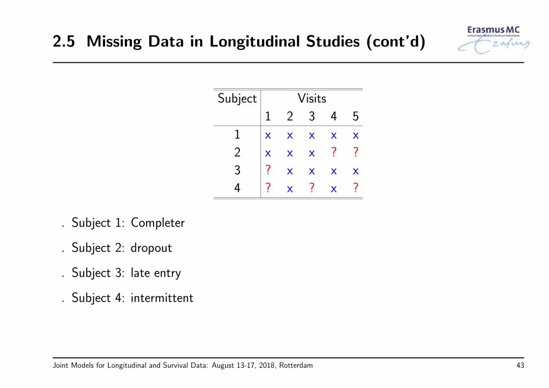
2.5 Missing Data in Longitudinal Studies (cont’d)
Subject Visits
1 2 3 4 5
1 x x x x x
2 x x x ? ?
3 ? x x x x
4 ? x ? x ?
Subject 1: Completer
Subject 2: dropout
Subject 3: late entry
Subject 4: intermittent
Joint Models for Longitudinal and Survival Data: August 13-17, 2018, Rotterdam 43

2.5 Missing Data in Longitudinal Studies (cont’d)
• Implications of missingness:
we collect less data than originally planned ⇒ loss of efficiency
not all subjects have the same number of measurements ⇒ unbalanced datasets
missingness may depend on outcome ⇒ potential bias
• For the handling of missing data, we introduce the missing data indicator
rij =
1 if yij is observed
0 otherwise
Joint Models for Longitudinal and Survival Data: August 13-17, 2018, Rotterdam 44

2.5 Missing Data in Longitudinal Studies (cont’d)
• We obtain a partition of the complete response vector yi
observed data yoi , containing those yij for which rij = 1
missing data ymi , containing those yij for which rij = 0
• For the remaining we will focus on dropout ⇒ notation can be simplified
Discrete dropout time: rdi = 1 +ni∑j=1
rij (ordinal variable)
Continuous time: T ∗i denotes the time to dropout
Joint Models for Longitudinal and Survival Data: August 13-17, 2018, Rotterdam 45

2.6 Missing Data Mechanisms
• To describe the probabilistic relation between the measurement and missingnessprocesses Rubin (1976, Biometrika) has introduced three mechanisms
• Missing Completely At Random (MCAR): The probability that responses are missingis unrelated to both yoi and y
mi
p(ri | yoi , ymi ) = p(ri)
• Examples
subjects go out of the study after providing a pre-determined number ofmeasurements
laboratory measurements are lost due to equipment malfunction
Joint Models for Longitudinal and Survival Data: August 13-17, 2018, Rotterdam 46

2.6 Missing Data Mechanisms (cont’d)
• Features of MCAR:
The observed data yoi can be considered a random sample of the complete data yi
We can use any statistical procedure that is valid for complete data
* sample averages per time point
* linear regression, ignoring the correlation (consistent, but not efficient)
* t-test at the last time point
* . . .
Joint Models for Longitudinal and Survival Data: August 13-17, 2018, Rotterdam 47
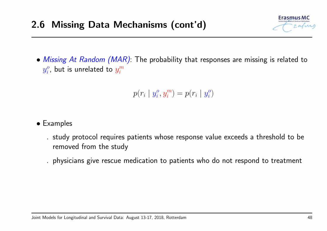
2.6 Missing Data Mechanisms (cont’d)
• Missing At Random (MAR): The probability that responses are missing is related toyoi , but is unrelated to ymi
p(ri | yoi , ymi ) = p(ri | yoi )
• Examples
study protocol requires patients whose response value exceeds a threshold to beremoved from the study
physicians give rescue medication to patients who do not respond to treatment
Joint Models for Longitudinal and Survival Data: August 13-17, 2018, Rotterdam 48

2.6 Missing Data Mechanisms (cont’d)
• Features of MAR:
The observed data cannot be considered a random sample from the targetpopulation
Not all statistical procedures provide valid results
Not valid under MAR Valid under MARsample marginal evolutions sample subject-specific evolutions
methods based on moments, likelihood based inferencesuch as GEE
mixed models with misspecified mixed models with correctly specifiedcorrelation structure correlation structure
marginal residuals subject-specific residuals
Joint Models for Longitudinal and Survival Data: August 13-17, 2018, Rotterdam 49

2.6 Missing Data Mechanisms (cont’d)
0 1 2 3 4 5
020
4060
80
MAR Missingness
Time
Long
itudi
nal O
utco
me
loess based on all data
Joint Models for Longitudinal and Survival Data: August 13-17, 2018, Rotterdam 50

2.6 Missing Data Mechanisms (cont’d)
0 1 2 3 4 5
020
4060
80
MAR Missingness
Time
Long
itudi
nal O
utco
me
observed
missing (previous y > 27)
loess based on all data
loess based on observed data
Joint Models for Longitudinal and Survival Data: August 13-17, 2018, Rotterdam 51
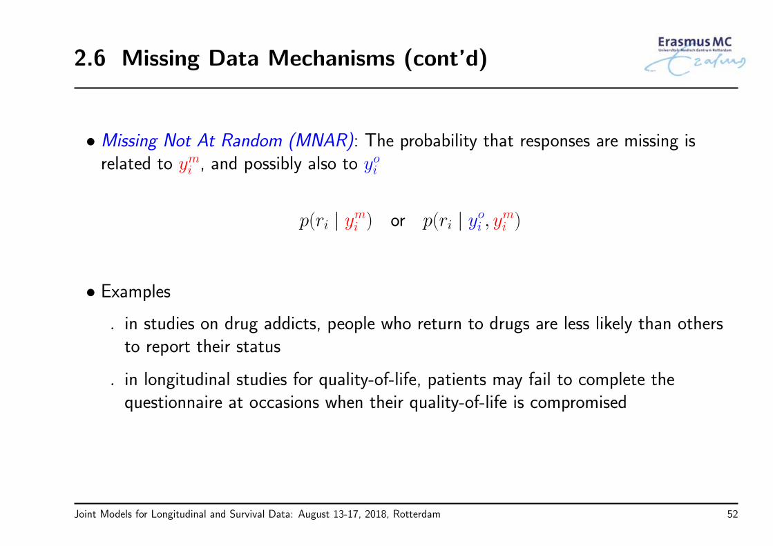
2.6 Missing Data Mechanisms (cont’d)
• Missing Not At Random (MNAR): The probability that responses are missing isrelated to ymi , and possibly also to yoi
p(ri | ymi ) or p(ri | yoi , ymi )
• Examples
in studies on drug addicts, people who return to drugs are less likely than othersto report their status
in longitudinal studies for quality-of-life, patients may fail to complete thequestionnaire at occasions when their quality-of-life is compromised
Joint Models for Longitudinal and Survival Data: August 13-17, 2018, Rotterdam 52
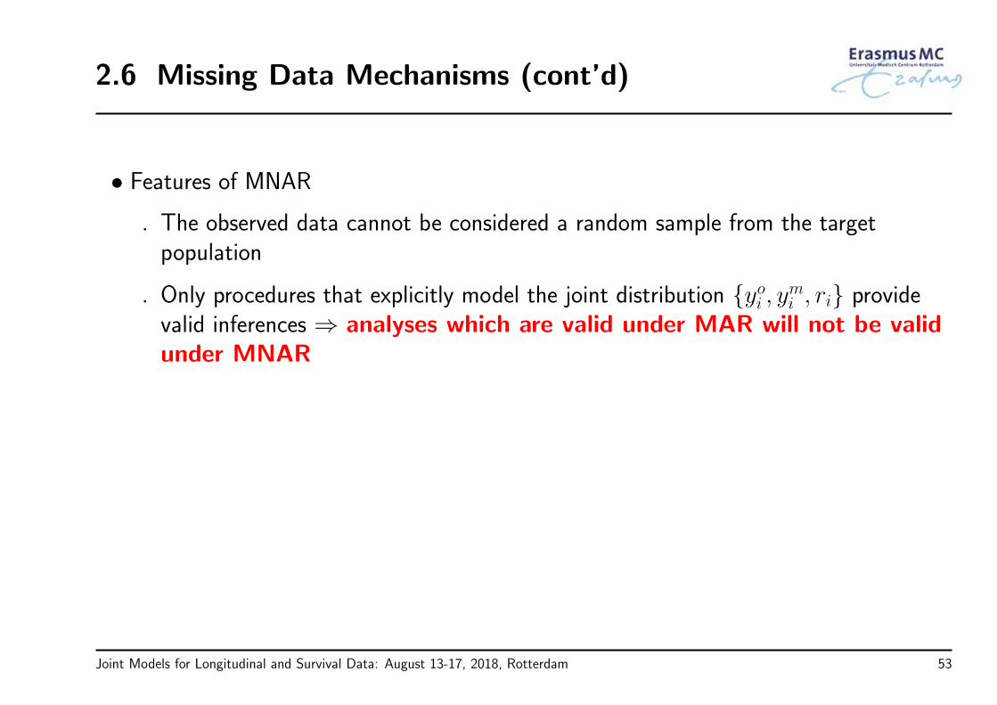
2.6 Missing Data Mechanisms (cont’d)
• Features of MNAR
The observed data cannot be considered a random sample from the targetpopulation
Only procedures that explicitly model the joint distribution yoi , ymi , ri providevalid inferences ⇒ analyses which are valid under MAR will not be validunder MNAR
Joint Models for Longitudinal and Survival Data: August 13-17, 2018, Rotterdam 53

2.6 Missing Data Mechanisms (cont’d)
We cannot tell from the data at hand whether themissing data mechanism is MAR or MNAR
Note: We can distinguish between MCAR and MAR
Joint Models for Longitudinal and Survival Data: August 13-17, 2018, Rotterdam 54

Part III
Relative Risk Models
Joint Models for Longitudinal and Survival Data: August 13-17, 2018, Rotterdam 55

3.1 Features of Survival Data
• The most important characteristic that distinguishes the analysis of time-to-eventoutcomes from other areas in statistics is Censoring
the event time of interest is not fully observed for all subjects under study
• Implications of censoring:
standard tools, such as the sample average, the t-test, and linear regressioncannot be used
inferences may be sensitive to misspecification of the distribution of the eventtimes
Joint Models for Longitudinal and Survival Data: August 13-17, 2018, Rotterdam 56

3.1 Features of Survival Data (cont’d)
• Several types of censoring:
Location of the true event time wrt the censoring time: right, left & interval
Probabilistic relation between the true event time & the censoring time:informative & non-informative (similar to MNAR and MAR)
Here we focus on non-informative right censoring
• Note: Survival times may often be truncated; analysis of truncated samples requiressimilar calculations as censoring
Joint Models for Longitudinal and Survival Data: August 13-17, 2018, Rotterdam 57

3.1 Features of Survival Data (cont’d)
• Notation (i denotes the subject)
T ∗i ‘true’ time-to-event
Ci the censoring time (e.g., the end of the study or a random censoring time)
• Available data for each subject
observed event time: Ti = min(T ∗i , Ci)
event indicator: δi = 1 if event; δi = 0 if censored
Our aim is to make valid inferences for T ∗i but using
only Ti, δi
Joint Models for Longitudinal and Survival Data: August 13-17, 2018, Rotterdam 58

3.2 Basic functions in Survival Analysis
• Hazard function: The instantaneous risk of an event at time t, given that the eventhas not occurred until t
h(t) = limdt→0
Pr(t ≤ T ∗ < t + dt | T ∗ ≥ t)
dt, t > 0
it is not a probability, i.e., h(t) ∈ (0,∞)
can be interpreted as the expected number of events per individual per unit of time
Joint Models for Longitudinal and Survival Data: August 13-17, 2018, Rotterdam 59
3.2 Basic functions in Survival Analysis (cont’d)
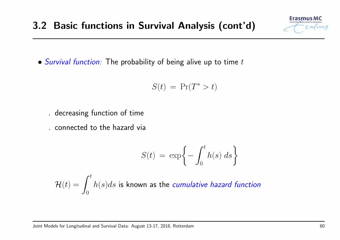
• Survival function: The probability of being alive up to time t
S(t) = Pr(T ∗ > t)
decreasing function of time
connected to the hazard via
S(t) = exp
−∫ t
0
h(s) ds
H(t) =
∫ t
0
h(s)ds is known as the cumulative hazard function
Joint Models for Longitudinal and Survival Data: August 13-17, 2018, Rotterdam 60

3.2 Basic functions in Survival Analysis (cont’d)
• Consistent estimates for the survival and cumulative hazard functions that accountfor censoring are provided by the
Kaplan-Meier estimator
SKM(t) =∏i:ti≤t
ri − diri
Nelson-Aalen estimator
HNA(t) =∑i:ti≤t
diri,
with ri # subjects still at risk at ti, and di # events at ti
Joint Models for Longitudinal and Survival Data: August 13-17, 2018, Rotterdam 61
3.3 Relative Risk Models
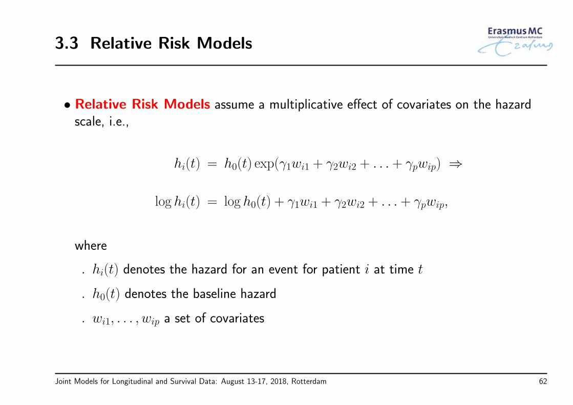
• Relative Risk Models assume a multiplicative effect of covariates on the hazardscale, i.e.,
hi(t) = h0(t) exp(γ1wi1 + γ2wi2 + . . . + γpwip) ⇒
log hi(t) = log h0(t) + γ1wi1 + γ2wi2 + . . . + γpwip,
where
hi(t) denotes the hazard for an event for patient i at time t
h0(t) denotes the baseline hazard
wi1, . . . , wip a set of covariates
Joint Models for Longitudinal and Survival Data: August 13-17, 2018, Rotterdam 62

3.3 Relative Risk Models (cont’d)
• The baseline hazard h0(t) represents the hazard for an event when all the covariatesor all the γs are 0
• That is, h0(t) represents the instantaneous risk of experiencing the event at time t,without the influence of any covariate
• Therefore,
if a covariate has a beneficial effect, decreases h0(t) → γ < 0
if it has a harmful effect, increases h0(t) → γ > 0
Joint Models for Longitudinal and Survival Data: August 13-17, 2018, Rotterdam 63

3.3 Relative Risk Models (cont’d)
• Standard MLE can be applied based on the log-likelihood function
ℓ(θ) =
n∑i=1
δi log p(Ti; θ) + (1− δi) log Si(Ti; θ),
which also can be re-expressed in terms of the hazard function
ℓ(θ) =
n∑i=1
δi log hi(Ti; θ)−∫ Ti
0
hi(s; θ) ds
Sensitivity to distributional assumptions due tocensoring
Joint Models for Longitudinal and Survival Data: August 13-17, 2018, Rotterdam 64
3.3 Relative Risk Models (cont’d)
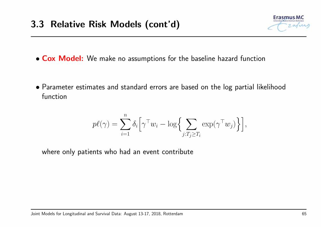
• Cox Model: We make no assumptions for the baseline hazard function
• Parameter estimates and standard errors are based on the log partial likelihoodfunction
pℓ(γ) =
n∑i=1
δi
[γ⊤wi − log
∑j:Tj≥Ti
exp(γ⊤wj)],
where only patients who had an event contribute
Joint Models for Longitudinal and Survival Data: August 13-17, 2018, Rotterdam 65

3.3 Relative Risk Models (cont’d)
• Example: For the PBC dataset were interested in the treatment effect whilecorrecting for sex and age effects
hi(t) = h0(t) exp(γ1D-penici + γ2Femalei + γ3Agei)
Value HR Std.Err. z-value p-value
γ1 −0.138 0.871 0.156 −0.882 0.378
γ2 −0.493 0.611 0.207 −2.379 0.017
γ3 0.021 1.022 0.008 2.784 0.005
Joint Models for Longitudinal and Survival Data: August 13-17, 2018, Rotterdam 66

3.4 Relative Risk Models in R
R> The primary package in R for the analysis of survival data is the survival package
R> A key function in this package that is used to specify the available event timeinformation in a sample at hand is Surv()
R> For right censored failure times (i.e., what we will see in this course) we need toprovide the observed event times time, and the event indicator status, whichequals 1 for true failure times and 0 for right censored times
Surv(time, status)
Joint Models for Longitudinal and Survival Data: August 13-17, 2018, Rotterdam 67

3.4 Relative Risk Models in R (cont’d)
R> Cox models are fitted using function coxph(). For instance, for the PBC data thefollowing code fits the Cox model that contains the main effects of ‘drug’, ‘sex’ and‘age’:
coxFit <- coxph(Surv(years, status2) ~ drug + sex + age,
data = pbc2.id)
summary(coxFit)
R> The two main arguments are a formula specifying the design matrix of the modeland a data frame containing all the variables
Joint Models for Longitudinal and Survival Data: August 13-17, 2018, Rotterdam 68

3.5 Time Dependent Covariates
• Often interest in the association between a time-dependent covariate and the risk foran event
treatment changes with time (e.g., dose)
time-dependent exposure (e.g., smoking, diet)
markers of disease or patient condition (e.g., blood pressure, PSA levels)
. . .
• Example: In the PBC study, are the longitudinal bilirubin measurements associatedwith the hazard for death?
Joint Models for Longitudinal and Survival Data: August 13-17, 2018, Rotterdam 69

3.5 Time Dependent Covariates (cont’d)
• To answer our questions of interest we need to postulate a model that relates
the serum bilirubin with
the time-to-death
• The association between baseline marker levels and the risk for death can beestimated with standard statistical tools (e.g., Cox regression)
• When we move to the time-dependent setting, a more careful consideration isrequired
Joint Models for Longitudinal and Survival Data: August 13-17, 2018, Rotterdam 70

3.5 Time Dependent Covariates (cont’d)
• There are two types of time-dependent covariates(Kalbfleisch and Prentice, 2002, Section 6.3)
Exogenous (aka external): the future path of the covariate up to any time t > s isnot affected by the occurrence of an event at time point s, i.e.,
PrYi(t) | Yi(s), T ∗
i ≥ s= Pr
Yi(t) | Yi(s), T ∗
i = s,
where 0 < s ≤ t and Yi(t) = yi(s), 0 ≤ s < t
Endogenous (aka internal): not Exogenous
Joint Models for Longitudinal and Survival Data: August 13-17, 2018, Rotterdam 71

3.5 Time Dependent Covariates (cont’d)
• It is very important to distinguish between these two types of time-dependentcovariates, because the type of covariate dictates the appropriate type of analysis
• In our motivating examples all time-varying covariates are Biomarkers ⇒ These arealways endogenous covariates
measured with error (i.e., biological variation)
the complete history is not available
existence directly related to failure status
Joint Models for Longitudinal and Survival Data: August 13-17, 2018, Rotterdam 72

3.5 Time Dependent Covariates (cont’d)
0 5 10 15 20
68
1012
Subject 127
Follow−up Time (months)
CD
4 ce
ll co
unt
Joint Models for Longitudinal and Survival Data: August 13-17, 2018, Rotterdam 73

3.6 Extended Cox Model
• The Cox model presented earlier can be extended to handle time-dependentcovariates using the counting process formulation
hi(t | Yi(t), wi) = h0(t)Ri(t) expγ⊤wi + αyi(t),
where
Ni(t) is a counting process which counts the number of events for subject i bytime t,
hi(t) denotes the intensity process for Ni(t),
Ri(t) denotes the at risk process (‘1’ if subject i still at risk at t), and
yi(t) denotes the value of the time-varying covariate at t
Joint Models for Longitudinal and Survival Data: August 13-17, 2018, Rotterdam 74

3.6 Extended Cox Model (cont’d)
• Interpretation:
hi(t | Yi(t), wi) = h0(t)Ri(t) expγ⊤wi + αyi(t)
exp(α) denotes the relative increase in the risk for an event at time t that resultsfrom one unit increase in yi(t) at the same time point
• Parameters are estimated based on the log-partial likelihood function
pℓ(γ, α) =
n∑i=1
∫ ∞
0
Ri(t) expγ⊤wi + αyi(t)
− log[∑
j
Rj(t) expγ⊤wj + αyj(t)]
dNi(t)
Joint Models for Longitudinal and Survival Data: August 13-17, 2018, Rotterdam 75

3.6 Extended Cox Model (cont’d)
• Typically, data must be organized in the long format
Patient Start Stop Event yi(t) Age
1 0 135 1 5.5 45
2 0 65 0 2.2 38
2 65 120 0 3.1 38
2 120 155 1 4.1 38
3 0 115 0 2.5 29
3 115 202 0 2.9 29... ... ... ... ... ...
Joint Models for Longitudinal and Survival Data: August 13-17, 2018, Rotterdam 76

3.6 Extended Cox Model (cont’d)
• How does the extended Cox model handle time-varying covariates?
assumes no measurement error
step-function path
existence of the covariate is not related to failure status
Joint Models for Longitudinal and Survival Data: August 13-17, 2018, Rotterdam 77

3.6 Extended Cox Model (cont’d)
Time
0.1
0.2
0.3
0.4
hazard function
−0.
50.
00.
51.
01.
52.
0
0 2 4 6 8 10
longitudinal outcome
Joint Models for Longitudinal and Survival Data: August 13-17, 2018, Rotterdam 78
3.6 Extended Cox Model (cont’d)
• Therefore, the extended Cox model is only valid for exogenous time-dependentcovariates
Treating endogenous covariates as exogenous mayproduce spurious results!
Joint Models for Longitudinal and Survival Data: August 13-17, 2018, Rotterdam 79

Part IV
The Basic Joint Model
Joint Models for Longitudinal and Survival Data: August 13-17, 2018, Rotterdam 80

4.1 Joint Modeling Framework
• To account for the special features of endogenous covariates a new class of modelshas been developed
Joint Models for Longitudinal and Time-to-Event Data
• Intuitive idea behind these models
1. use an appropriate model to describe the evolution of the marker in time for eachpatient
2. the estimated evolutions are then used in a Cox model
• Feature: Marker level’s are not assumed constant between visits
Joint Models for Longitudinal and Survival Data: August 13-17, 2018, Rotterdam 81

4.1 Joint Modeling Framework (cont’d)
Time
0.1
0.2
0.3
0.4
hazard function
−0.
50.
00.
51.
01.
52.
0
0 2 4 6 8 10
longitudinal outcome
Joint Models for Longitudinal and Survival Data: August 13-17, 2018, Rotterdam 82

4.1 Joint Modeling Framework (cont’d)
• Some notation
T ∗i : True event time for patient i
Ti: Observed event time for patient i
δi: Event indicator, i.e., equals 1 for true events
yi: Longitudinal responses
• We will formulate the joint model in 3 steps – in particular, . . .
Joint Models for Longitudinal and Survival Data: August 13-17, 2018, Rotterdam 83

4.1 Joint Modeling Framework (cont’d)
• Step 1: Let’s assume that we know mi(t), i.e., the true & unobserved value of themarker at time t
• Then, we can define a standard relative risk model
hi(t | Mi(t)) = h0(t) expγ⊤wi + αmi(t),
where
Mi(t) = mi(s), 0 ≤ s < t longitudinal history
α quantifies the strength of the association between the marker and the risk foran event
wi baseline covariates
Joint Models for Longitudinal and Survival Data: August 13-17, 2018, Rotterdam 84
4.1 Joint Modeling Framework (cont’d)
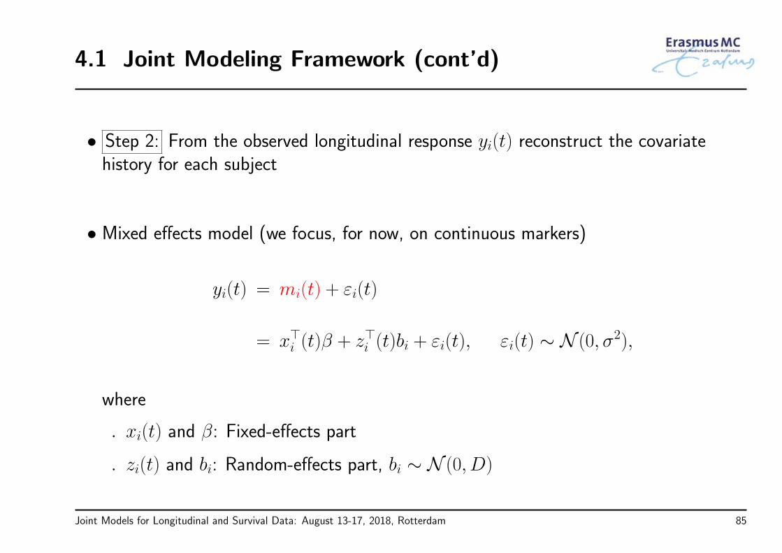
• Step 2: From the observed longitudinal response yi(t) reconstruct the covariatehistory for each subject
• Mixed effects model (we focus, for now, on continuous markers)
yi(t) = mi(t) + εi(t)
= x⊤i (t)β + z⊤i (t)bi + εi(t), εi(t) ∼ N (0, σ2),
where
xi(t) and β: Fixed-effects part
zi(t) and bi: Random-effects part, bi ∼ N (0, D)
Joint Models for Longitudinal and Survival Data: August 13-17, 2018, Rotterdam 85

4.1 Joint Modeling Framework (cont’d)
• Step 3: The two processes are associated ⇒ define a model for their jointdistribution
• Joint Models for such joint distributions are of the following form(Tsiatis & Davidian, Stat. Sinica, 2004)
p(yi, Ti, δi) =
∫p(yi | bi)
h(Ti | bi)δi S(Ti | bi)
p(bi) dbi,
where
bi a vector of random effects that explains the interdependencies
p(·) density function; S(·) survival function
Joint Models for Longitudinal and Survival Data: August 13-17, 2018, Rotterdam 86

4.1 Joint Modeling Framework (cont’d)
• Key assumption: Full Conditional Independence ⇒ random effects explain allinterdependencies
the longitudinal outcome is independent of the time-to-event outcome
the repeated measurements in the longitudinal outcome are independent of eachother
p(yi, Ti, δi | bi) = p(yi | bi) p(Ti, δi | bi)
p(yi | bi) =∏j
p(yij | bi)
Caveat: CI is difficult to be tested
Joint Models for Longitudinal and Survival Data: August 13-17, 2018, Rotterdam 87

4.1 Joint Modeling Framework (cont’d)
• The censoring and visiting∗ processes are assumed non-informative:
• Decision to withdraw from the study or appear for the next visit
may depend on observed past history (baseline covariates + observedlongitudinal responses)
no additional dependence on underlying, latent subject characteristicsassociated with prognosis
∗The visiting process is defined as the mechanism (stochastic or deterministic) that generates the time points at which
longitudinal measurements are collected.
Joint Models for Longitudinal and Survival Data: August 13-17, 2018, Rotterdam 88

4.1 Joint Modeling Framework (cont’d)
• The survival function, which is a part of the likelihood of the model, depends on thewhole longitudinal history
Si(t | bi) = exp
(−∫ t
0
h0(s) expγ⊤wi + αmi(s) ds)
• Therefore, care in the definition of the design matrices of the mixed model
when subjects have nonlinear profiles ⇒
use splines or polynomials to model them flexibly
Joint Models for Longitudinal and Survival Data: August 13-17, 2018, Rotterdam 89

4.1 Joint Modeling Framework (cont’d)
• Random-effects distribution
in mixed models it is customary to assume normality (see p. 85);
however, in joint models this distribution plays a more prominent role because therandom effects explain all associations (see p. 87);
nevertheless, robustness, especially as ni increases (see Rizopoulos et al., 2008, Biometrika)
Joint Models for Longitudinal and Survival Data: August 13-17, 2018, Rotterdam 90

4.1 Joint Modeling Framework (cont’d)
• Assumptions for the baseline hazard function h0(t)
parametric ⇒ possibly restrictive
unspecified ⇒ within JM framework underestimates standard errors
• It is advisable to use parametric but flexible models for h0(t)
splines
log h0(t) = γh0,0 +
Q∑q=1
γh0,qBq(t, v),
where
* Bq(t, v) denotes the q-th basis function of a B-spline with knots v1, . . . , vQ
* γh0 a vector of spline coefficients
Joint Models for Longitudinal and Survival Data: August 13-17, 2018, Rotterdam 91

4.1 Joint Modeling Framework (cont’d)
• It is advisable to use parametric but flexible models for h0(t)
step-functions: piecewise-constant baseline hazard often works satisfactorily
h0(t) =
Q∑q=1
ξqI(vq−1 < t ≤ vq),
where 0 = v0 < v1 < · · · < vQ denotes a split of the time scale
Joint Models for Longitudinal and Survival Data: August 13-17, 2018, Rotterdam 92
4.2 Estimation
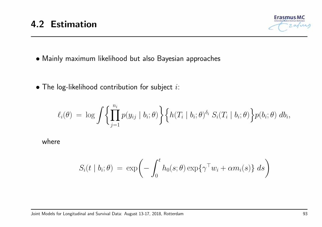
• Mainly maximum likelihood but also Bayesian approaches
• The log-likelihood contribution for subject i:
ℓi(θ) = log
∫ ni∏j=1
p(yij | bi; θ)
h(Ti | bi; θ)δi Si(Ti | bi; θ)p(bi; θ) dbi,
where
Si(t | bi; θ) = exp
(−∫ t
0
h0(s; θ) expγ⊤wi + αmi(s) ds)
Joint Models for Longitudinal and Survival Data: August 13-17, 2018, Rotterdam 93

4.2 Estimation (cont’d)
• Both integrals do not have, in general, a closed-form solution ⇒ need to beapproximated numerically
• Standard numerical integration algorithms
Gaussian quadrature
Monte Carlo
. . .
• More difficult is the integral with respect to bi because it can be of high dimension
Laplace approximations
pseudo-adaptive Gaussian quadrature rules
Joint Models for Longitudinal and Survival Data: August 13-17, 2018, Rotterdam 94

4.2 Estimation (cont’d)
• To maximize the approximated log-likelihood
ℓ(θ) =
n∑i=1
log
∫p(yi | bi; θ)
h(Ti | bi; θ)δi Si(Ti | bi; θ)
p(bi; θ) dbi,
we need to employ an optimization algorithm
• Standard choices
EM (treating bi as missing data)
Newton-type
hybrids (start with EM and continue with quasi-Newton)
Joint Models for Longitudinal and Survival Data: August 13-17, 2018, Rotterdam 95

4.2 Estimation (cont’d)
• Standard errors: Standard asymptotic MLE
var(θ) =
−
n∑i=1
∂2 log p(yi, Ti, δi; θ)
∂θ⊤∂θ
∣∣∣θ=θ
−1
• Standard asymptotic tests + information criteria
likelihood ratio test
score test
Wald test
AIC, BIC, . . .
Joint Models for Longitudinal and Survival Data: August 13-17, 2018, Rotterdam 96

4.2 Estimation (cont’d)
• Based on a fitted joint model, estimates for the random effects are based on theposterior distribution:
p(bi | Ti, δi, yi; θ) =p(Ti, δi | bi; θ) p(yi | bi; θ) p(bi; θ)
p(Ti, δi, yi; θ)
∝ p(Ti, δi | bi; θ) p(yi | bi; θ) p(bi; θ),
in which θ is replaced by its MLE θ
Joint Models for Longitudinal and Survival Data: August 13-17, 2018, Rotterdam 97
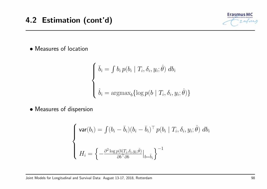
4.2 Estimation (cont’d)
• Measures of location bi =
∫bi p(bi | Ti, δi, yi; θ) dbi
bi = argmaxblog p(b | Ti, δi, yi; θ)
• Measures of dispersion
var(bi) =
∫(bi − bi)(bi − bi)
⊤ p(bi | Ti, δi, yi; θ) dbi
Hi =−∂2 log p(b|Ti,δi,yi;θ)
∂b⊤∂b
∣∣b=bi
−1
Joint Models for Longitudinal and Survival Data: August 13-17, 2018, Rotterdam 98

4.3 Bayesian Estimation
• Bayesian estimation
under the Bayesian paradigm both θ and bi, i = 1, . . . , n are regarded asparameters
• Inference is based on the full posterior distribution
p(θ, b | T, δ, y) =
∏i p(Ti, δi | bi; θ) p(yi | bi; θ) p(bi; θ) p(θ)∏
i p(Ti, δi, yi)
∝n∏i=1
p(Ti, δi | bi; θ) p(yi | bi; θ) p(bi; θ)
p(θ)
Joint Models for Longitudinal and Survival Data: August 13-17, 2018, Rotterdam 99

4.3 Bayesian Estimation (cont’d)
• No closed-form solutions for the integrals in the normalizing constant ⇒ MCMC
• For the standard joint model we have define thus far, the majority of the parameterscan be updated using Gibbs sampling (or slice sampling)
when no close-form posterior conditionals are available, we can use theMetropolis-Hastings algorithm
• To gain in efficiency, we can do block-updating for many of the parameters, i.e.,
fixed effects β
random effects bi
baseline covariates in the survival submodel γ
Joint Models for Longitudinal and Survival Data: August 13-17, 2018, Rotterdam 100

4.3 Bayesian Estimation (cont’d)
• Good proposal distributions can be obtained from the separate fits of the twosubmodels
• Not directly programmable in WinBUGS, INLA, etc., due to the integral in thedefinition of the survival function
Si(t | bi; θ) = exp
(−∫ t
0
h0(s; θ) expγ⊤wi + αmi(s) ds)
extra steps required. . .
Joint Models for Longitudinal and Survival Data: August 13-17, 2018, Rotterdam 101

4.3 Bayesian Estimation (cont’d)
• Inference then proceeds in the usual manner from the MCMC output, e.g.,
posterior means, variances, and standard errors
credible intervals
Bayes factors
DIC, CPO
. . .
Joint Models for Longitudinal and Survival Data: August 13-17, 2018, Rotterdam 102

4.4 A Comparison with the TD Cox
• Example: To illustrate the virtues of joint modeling, we compare it with the standardtime-dependent Cox model for the AIDS data
yi(t) = mi(t) + εi(t)
= β0 + β1t + β2t× ddIi + bi0 + bi1t + εi(t), εi(t) ∼ N (0, σ2),
hi(t) = h0(t) expγddIi + αmi(t),
where
h0(t) is assumed piecewise-constant
Joint Models for Longitudinal and Survival Data: August 13-17, 2018, Rotterdam 103
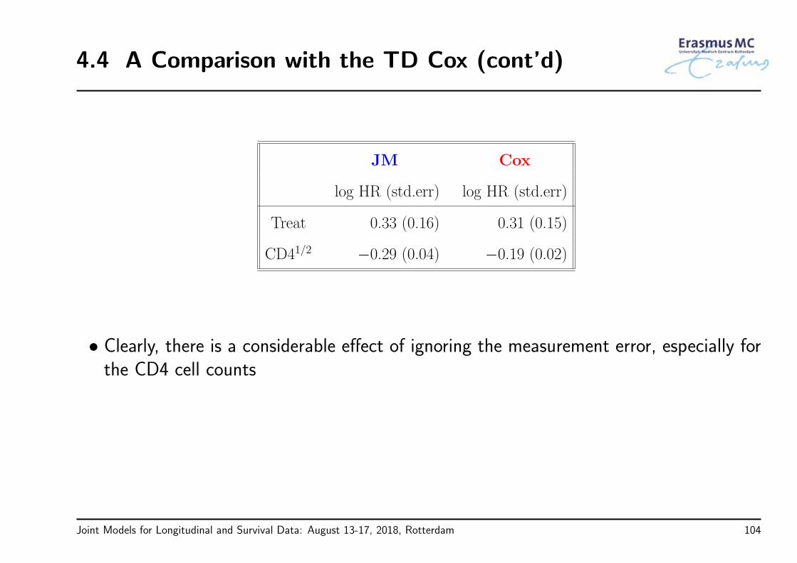
4.4 A Comparison with the TD Cox (cont’d)
JM Cox
log HR (std.err) log HR (std.err)
Treat 0.33 (0.16) 0.31 (0.15)
CD41/2 −0.29 (0.04) −0.19 (0.02)
• Clearly, there is a considerable effect of ignoring the measurement error, especially forthe CD4 cell counts
Joint Models for Longitudinal and Survival Data: August 13-17, 2018, Rotterdam 104

4.4 A Comparison with the TD Cox (cont’d)
• A unit decrease in CD41/2, results in a
Joint Model: 1.3-fold increase in risk (95% CI: 1.24; 1.43)
Time-Dependent Cox: 1.2-fold increase in risk (95% CI: 1.16; 1.27)
• Which one to believe?
a lot of theoretical and simulation work has shown that the Cox modelunderestimates the true association size of markers
Joint Models for Longitudinal and Survival Data: August 13-17, 2018, Rotterdam 105

4.5 Joint Models in R
R> Joint models are fitted using function jointModel() from package JM. Thisfunction accepts as main arguments a linear mixed model and a Cox PH model basedon which it fits the corresponding joint model
lmeFit <- lme(CD4 ~ obstime + obstime:drug,
random = ~ obstime | patient, data = aids)
coxFit <- coxph(Surv(Time, death) ~ drug, data = aids.id, x = TRUE)
jointFit <- jointModel(lmeFit, coxFit, timeVar = "obstime",
method = "piecewise-PH-aGH")
summary(jointFit)
Joint Models for Longitudinal and Survival Data: August 13-17, 2018, Rotterdam 106

4.5 Joint Models in R (cont’d)
R> As before, the data frame given in lme() should be in the long format, while thedata frame given to coxph() should have one line per subject∗
the ordering of the subjects needs to be the same
R> In the call to coxph() you need to set x = TRUE (or model = TRUE) such thatthe design matrix used in the Cox model is returned in the object fit
R> Argument timeVar specifies the time variable in the linear mixed model
∗ Unless you want to include exogenous time-varying covariates or handle competing risks
Joint Models for Longitudinal and Survival Data: August 13-17, 2018, Rotterdam 107

4.5 Joint Models in R (cont’d)
R> Argument method specifies the type of relative risk model and the type of numericalintegration algorithm – the syntax is as follows:
<baseline hazard>-<parameterization>-<numerical integration>
Available options are:
"piecewise-PH-GH": PH model with piecewise-constant baseline hazard
"spline-PH-GH": PH model with B-spline-approximated log baseline hazard
"weibull-PH-GH": PH model with Weibull baseline hazard
"weibull-AFT-GH": AFT model with Weibull baseline hazard
"Cox-PH-GH": PH model with unspecified baseline hazard
GH stands for standard Gauss-Hermite; using aGH invokes the pseudo-adaptiveGauss-Hermite rule
Joint Models for Longitudinal and Survival Data: August 13-17, 2018, Rotterdam 108

4.5 Joint Models in R (cont’d)
R> Joint models under the Bayesian approach are fitted using functionjointModelBayes() from package JMbayes. This function works in a very similarmanner as function jointModel(), e.g.,
lmeFit <- lme(CD4 ~ obstime + obstime:drug,
random = ~ obstime | patient, data = aids)
coxFit <- coxph(Surv(Time, death) ~ drug, data = aids.id, x = TRUE)
jointFitBayes <- jointModelBayes(lmeFit, coxFit, timeVar = "obstime")
summary(jointFitBayes)
Joint Models for Longitudinal and Survival Data: August 13-17, 2018, Rotterdam 109
4.5 Joint Models in R (cont’d)
R> JMbayes is more flexible (in some respects):
directly implements the MCMC
allows for categorical longitudinal data as well
allows for general transformation functions
penalized B-splines for the baseline hazard function
. . .
Joint Models for Longitudinal and Survival Data: August 13-17, 2018, Rotterdam 110

4.5 Joint Models in R (cont’d)
R> In both packages methods are available for the majority of the standard genericfunctions + extras
summary(), anova(), vcov(), logLik()
coef(), fixef(), ranef()
fitted(), residuals()
plot()
xtable() (you need to load package xtable first)
Joint Models for Longitudinal and Survival Data: August 13-17, 2018, Rotterdam 111

4.6 Connection with Missing Data
• So far we have attacked the problem from the survival point of view
• However, often, we may be also interested on the longitudinal outcome
• Issue: When patients experience the event, they dropout from the study
a direct connection with the missing data field
Dropout must be taken into account when derivinginferences for the longitudinal outcome
Joint Models for Longitudinal and Survival Data: August 13-17, 2018, Rotterdam 112

4.6 Connection with Missing Data (cont’d)
• To show this connection more clearly
T ∗i : true time-to-event
yoi : longitudinal measurements before T∗i
ymi : longitudinal measurements after T∗i
• Important to realize that the model we postulate for the longitudinal responses isfor the complete vector yoi , ymi
implicit assumptions about missingness
Joint Models for Longitudinal and Survival Data: August 13-17, 2018, Rotterdam 113

4.6 Connection with Missing Data (cont’d)
• Missing data mechanism:
p(T ∗i | yoi , ymi ) =
∫p(T ∗
i | bi) p(bi | yoi , ymi ) dbi
still depends on ymi , which corresponds to nonrandom dropout
Intuitive interpretation: Patients who dropout showdifferent longitudinal evolutions than patients who do not
Joint Models for Longitudinal and Survival Data: August 13-17, 2018, Rotterdam 114
4.6 Connection with Missing Data (cont’d)
• Implications of nonrandom dropout
observed data do not constitute a random sample from the target population
• This feature complicates the validation of the joint model’s assumptions usingstandard residual plots
what is the problem: Residual plots may show systematic behavior due to dropoutand not because of model misfit
Joint Models for Longitudinal and Survival Data: August 13-17, 2018, Rotterdam 115

4.6 Connection with Missing Data (cont’d)
• What about censoring?
censoring also corresponds to a discontinuation of the data collection process forthe longitudinal outcome
• Likelihood-based inferences for joint models provide valid inferences when censoring isMAR
a patient relocates to another country (MCAR)
a patient is excluded from the study when her longitudinal response exceeds aprespecified threshold (MAR)
censoring depends on random effects (MNAR)
Joint Models for Longitudinal and Survival Data: August 13-17, 2018, Rotterdam 116

4.6 Connection with Missing Data (cont’d)
• Joint models belong to the class of Shared Parameter Models
p(yoi , ymi , T
∗i ) =
∫p(yoi , y
mi | bi) p(T ∗
i | bi) p(bi)dbi
the association between the longitudinal and missingness processes is explained bythe shared random effects bi
Joint Models for Longitudinal and Survival Data: August 13-17, 2018, Rotterdam 117

4.6 Connection with Missing Data (cont’d)
• The other two well-known frameworks for MNAR data are
Selection models
p(yoi , ymi , T
∗i ) = p(yoi , y
mi ) p(T
∗i | yoi , ymi )
Pattern mixture models:
p(yoi , ymi , T
∗i ) = p(yoi , y
mi | T ∗
i ) p(T∗i )
• These two model families are primarily applied with discrete dropout times andcannot be easily extended to continuous time
Joint Models for Longitudinal and Survival Data: August 13-17, 2018, Rotterdam 118

4.6 Connection with Missing Data (cont’d)
• A nice feature of joint models / shared parameter models is that they can‘automatically’ handle intermittent missing data – the observed data likelihoodcontributions take the form:
p(yoi , T∗i ) =
∫p(yoi , y
mi , T
∗i ) dy
mi
=
∫ ∫p(yoi , y
mi | bi) p(T ∗
i | bi) p(bi) dbidymi
=
∫ ∫p(yoi , y
mi | bi) dymi
p(T ∗
i | bi) p(bi) dbi
=
∫p(yoi | bi) p(T ∗
i | bi) p(bi) dbi
This is not the case for selection and pattern mixture models!
Joint Models for Longitudinal and Survival Data: August 13-17, 2018, Rotterdam 119

4.6 Connection with Missing Data (cont’d)
• Example: In the AIDS data the association parameter α was highly significant,suggesting nonrandom dropout
• A comparison between
linear mixed-effects model ⇒ MAR
joint model ⇒ MNAR
is warranted
• MAR assumes that missingness depends only on the observed data
p(T ∗i | yoi , ymi ) = p(T ∗
i | yoi )
Joint Models for Longitudinal and Survival Data: August 13-17, 2018, Rotterdam 120
4.6 Connection with Missing Data (cont’d)
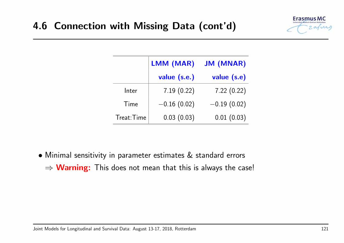
LMM (MAR) JM (MNAR)
value (s.e.) value (s.e)
Inter 7.19 (0.22) 7.22 (0.22)
Time −0.16 (0.02) −0.19 (0.02)
Treat:Time 0.03 (0.03) 0.01 (0.03)
• Minimal sensitivity in parameter estimates & standard errors
⇒ Warning: This does not mean that this is always the case!
Joint Models for Longitudinal and Survival Data: August 13-17, 2018, Rotterdam 121
Part V
Extensions of Joint Models
Joint Models for Longitudinal and Survival Data: August 13-17, 2018, Rotterdam 122

5.1 Parameterizations
• The standard joint model
hi(t | Mi(t)) = h0(t) expγ⊤wi + αmi(t),
yi(t) = mi(t) + εi(t)
= x⊤i (t)β + z⊤i (t)bi + εi(t),
where Mi(t) = mi(s), 0 ≤ s < t
Joint Models for Longitudinal and Survival Data: August 13-17, 2018, Rotterdam 123

5.1 Parameterizations (cont’d)
Time
0.1
0.2
0.3
0.4
hazard function
−0.
50.
00.
51.
01.
52.
0
0 2 4 6 8 10
longitudinal outcome
Joint Models for Longitudinal and Survival Data: August 13-17, 2018, Rotterdam 124

5.1 Parameterizations (cont’d)
• The standard joint model
hi(t | Mi(t)) = h0(t) expγ⊤wi + αmi(t),
yi(t) = mi(t) + εi(t)
= x⊤i (t)β + z⊤i (t)bi + εi(t),
where Mi(t) = mi(s), 0 ≤ s < t
Is this the only option? Is this the mostoptimal choice?
Joint Models for Longitudinal and Survival Data: August 13-17, 2018, Rotterdam 125

5.1 Parameterizations (cont’d)
• Note: Inappropriate modeling of time-dependent covariates may result in surprisingresults
• Example: Cavender et al. (1992, J. Am. Coll. Cardiol.) conducted an analysis totest the effect of cigarette smoking on survival of patients who underwent coronaryartery surgery
the estimated effect of current cigarette smoking was positive on survival althoughnot significant (i.e., patient who smoked had higher probability of survival)
most of those who had died were smokers but many stopped smoking at the lastfollow-up before their death
Joint Models for Longitudinal and Survival Data: August 13-17, 2018, Rotterdam 126
5.1 Parameterizations (cont’d)
We need to carefully consider the functional form oftime-dependent covariates
• Let’s see some possibilities. . .
Joint Models for Longitudinal and Survival Data: August 13-17, 2018, Rotterdam 127

5.1 Parameterizations (cont’d)
• Lagged Effects: The hazard for an event at t is associated with the level of themarker at a previous time point:
hi(t | Mi(t)) = h0(t) expγ⊤wi + αmi(tc+),
where
tc+ = max(t− c, 0)
Joint Models for Longitudinal and Survival Data: August 13-17, 2018, Rotterdam 128

5.1 Parameterizations (cont’d)
Time
0.1
0.2
0.3
0.4
hazard function
−0.
50.
00.
51.
01.
52.
0
0 2 4 6 8 10
longitudinal outcome
Joint Models for Longitudinal and Survival Data: August 13-17, 2018, Rotterdam 129

5.1 Parameterizations (cont’d)
• Time-dependent Slopes: The hazard for an event at t is associated with both thecurrent value and the slope of the trajectory at t (Ye et al., 2008, Biometrics):
hi(t | Mi(t)) = h0(t) expγ⊤wi + α1mi(t) + α2m′i(t),
where
m′i(t) =
d
dtx⊤i (t)β + z⊤i (t)bi
Joint Models for Longitudinal and Survival Data: August 13-17, 2018, Rotterdam 130

5.1 Parameterizations (cont’d)
Time
0.1
0.2
0.3
0.4
hazard function
−0.
50.
00.
51.
01.
52.
0
0 2 4 6 8 10
longitudinal outcome
Joint Models for Longitudinal and Survival Data: August 13-17, 2018, Rotterdam 131

5.1 Parameterizations (cont’d)
• Cumulative Effects: The hazard for an event at t is associated with the whole areaunder the trajectory up to t:
hi(t | Mi(t)) = h0(t) expγ⊤wi + α
∫ t
0
mi(s) ds
• Area under the longitudinal trajectory taken as a summary of Mi(t)
Joint Models for Longitudinal and Survival Data: August 13-17, 2018, Rotterdam 132

5.1 Parameterizations (cont’d)
Time
0.1
0.2
0.3
0.4
hazard function
−0.
50.
00.
51.
01.
52.
0
0 2 4 6 8 10
longitudinal outcome
Joint Models for Longitudinal and Survival Data: August 13-17, 2018, Rotterdam 133

5.1 Parameterizations (cont’d)
• Weighted Cumulative Effects (convolution): The hazard for an event at t isassociated with the area under the weighted trajectory up to t:
hi(t | Mi(t)) = h0(t) expγ⊤wi + α
∫ t
0
ϖ(t− s)mi(s) ds,
where ϖ(·) an appropriately chosen weight function, e.g.,
Gaussian density
Student’s-t density
. . .
Joint Models for Longitudinal and Survival Data: August 13-17, 2018, Rotterdam 134

5.1 Parameterizations (cont’d)
• Random Effects: The hazard for an event at t is associated only with the randomeffects of the longitudinal model:
hi(t | Mi(t)) = h0(t) exp(γ⊤wi + α⊤bi)
• Features:
avoids numerical integration for the survival function
interpretation of α more difficult, especially in high-dimensional random-effectssettings
Joint Models for Longitudinal and Survival Data: August 13-17, 2018, Rotterdam 135

5.1 Parameterizations (cont’d)
• Example: Sensitivity of inferences for the longitudinal process to the choice of theparameterization for the AIDS data
• We use the same mixed model as before, i.e.,
yi(t) = mi(t) + εi(t)
= β0 + β1t + β2t× ddIi + bi0 + bi1t + εi(t)
and the following four survival submodels
Joint Models for Longitudinal and Survival Data: August 13-17, 2018, Rotterdam 136

5.1 Parameterizations (cont’d)
• Model I (current value)
hi(t) = h0(t) expγddIi + α1mi(t)
• Model II (current value + current slope)
hi(t) = h0(t) expγddIi + α1mi(t) + α2m′i(t),
where
m′i(t) = β1 + β2ddIi + bi1
Joint Models for Longitudinal and Survival Data: August 13-17, 2018, Rotterdam 137

5.1 Parameterizations (cont’d)
• Model III (random slope)
hi(t) = h0(t) expγddIi + α3bi1
• Model IV (area)
hi(t) = h0(t) expγddIi + α4
∫ t
0
mi(s) ds,
where
∫ t0 mi(s) ds = β0t +
β12 t
2 + β22 t
2 × ddIi + bi0t +bi12 t
2
Joint Models for Longitudinal and Survival Data: August 13-17, 2018, Rotterdam 138

5.1 Parameterizations (cont’d)
Value
value
value+slope
random slope
area
6.8 7.0 7.2 7.4 7.6
β0
−0.25 −0.20 −0.15 −0.10
β1
−0.05 0.00 0.05
β2
Joint Models for Longitudinal and Survival Data: August 13-17, 2018, Rotterdam 139
5.1 Parameterizations (cont’d)
• There are noticeable differences between the parameterizations
especially in the slope parameters
• Therefore, a sensitivity analysis should not stop at the standard joint modelparameterization but also consider alternative association structures
Joint Models for Longitudinal and Survival Data: August 13-17, 2018, Rotterdam 140

5.1 Parameterizations (cont’d)
R> Lagged effects can be fitted using the lag argument of jointModel(). Forexample, the following code fits a joint model for the PBC dataset with
random intercepts and random slopes for log serum bilirubin, and
a relative risk model with piecewise-constant baseline hazard and the true effectat the previous year
lmeFit <- lme(log(serBilir) ~ year, random = ~ year | id, data = pbc2)
coxFit <- coxph(Surv(years, status2) ~ 1, data = pbc2.id, x = TRUE)
jointFit <- jointModel(lmeFit, coxFit, timeVar = "year",
method = "piecewise-PH-aGH", lag = 1)
summary(jointFit)
Joint Models for Longitudinal and Survival Data: August 13-17, 2018, Rotterdam 141

5.1 Parameterizations (cont’d)
R> For the time-dependent slopes and cumulative effects parameterizations, argumentsparameterization and derivForm of jointModel() should be used
the first one just specifies whether we want to include a single or two termsinvolving mi(t) in the linear predictor of the survival submodel, options are
* parameterization = "value"
* parameterization = "slope"
* parameterization = "both"
the second one requires a few extra steps to specify – we will see an example inthe practical
Joint Models for Longitudinal and Survival Data: August 13-17, 2018, Rotterdam 142
5.2 Latent Class Joint Models
• In many settings it may not be reasonable to assume that the population under studyis homogeneous
• Heterogeneity attributed to factors we have recorded
stratified analysis
• Heterogeneity attributed to factors we have not recorded
mixture models (aka latent class models)
Joint Models for Longitudinal and Survival Data: August 13-17, 2018, Rotterdam 143

5.2 Latent Class Joint Models (cont’d)
• Latent class joint model: We assume that the association between the longitudinaland event time processes is explained by some latent population heterogeneity
• Let G sub-populations, and ci = 1, . . . , G the latent sub-population indicator of theith subject in the sample
• Conditional independence:
p(Ti, δi, yi | ci = g, bi; θ) = p(Ti, δi | ci = g; θ) p(yi | ci = g, bi; θ)
p(yi | ci = g, bi; θ) =∏j
p(yij | ci = g, bi; θ)
Joint Models for Longitudinal and Survival Data: August 13-17, 2018, Rotterdam 144

5.2 Latent Class Joint Models (cont’d)
hi(t | ci = g) = h0g(t) exp(γ⊤g wi),
yi(t) | ci = g = x⊤i (t)βg + z⊤i (t)big + εi(t), big ∼ N (µg, σ2gD),
Pr(ci = g) = exp(λ⊤g ui)/∑G
l=1 exp(λ⊤l ui)
• The latent class joint models consists of three parts:
stratified relative risk model
heterogeneity linear mixed model
multinomial model for class membership
Joint Models for Longitudinal and Survival Data: August 13-17, 2018, Rotterdam 145
5.2 Latent Class Joint Models (cont’d)
• Features:
avoids numerical integration
local maxima
requires multiple fits to find the optimal number of classes (typically chosen usinginformation criteria)
no association parameter ⇒ no straightforward interpretation
Joint Models for Longitudinal and Survival Data: August 13-17, 2018, Rotterdam 146

5.2 Latent Class Joint Models (cont’d)
• Example: Latent class joint model analysis of the AIDS dataset
longitudinal submodel: random intercepts and random slopes with class-specificfixed effects
survival submodel: class-specific baseline risk & treatment effects
class membership submodel: treatment effect
• We fitted the models with 2, 3, 4, and 5 classes
Joint Models for Longitudinal and Survival Data: August 13-17, 2018, Rotterdam 147

5.2 Latent Class Joint Models (cont’d)
# Classes logLik AIC BIC
2 −4258.74 8565.48 8665.00
3 −4223.03 8516.06 8661.18
4 −4198.63 8489.26 8679.99
5 −4192.98 8499.96 8736.30
• AIC favors the 4-class model, whereas BIC chooses the 3-class solution
• Empirical studies suggest that the BIC more often finds the correct number of latentsubgroups
Joint Models for Longitudinal and Survival Data: August 13-17, 2018, Rotterdam 148
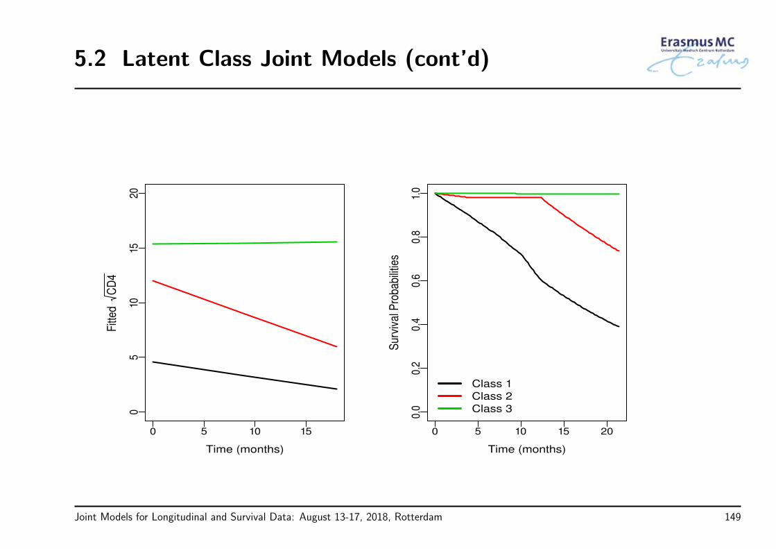
5.2 Latent Class Joint Models (cont’d)
0 5 10 15
05
1015
20
Time (months)
Fitt
ed
CD
4
0 5 10 15 20
0.0
0.2
0.4
0.6
0.8
1.0
Time (months)
Sur
viva
l Pro
babi
litie
sClass 1
Class 2
Class 3
Joint Models for Longitudinal and Survival Data: August 13-17, 2018, Rotterdam 149

5.2 Latent Class Joint Models (cont’d)
R> Latent class joint models can be fitted in R using function Jointlcmm() frompackage lcmm
lcjmFit.aids <- Jointlcmm(fixed = CD4 ~ obstime + drug,
mixture = ~ obstime + drug, random = ~ obstime,
classmb = ~ drug, subject = "patient", ng = 3, data = aids,
survival = Surv(Time, death) ~ mixture(drug),
hazard = "6-quant-piecewise", hazardtype = "Specific")
summary(lcjmFit.aids)
Joint Models for Longitudinal and Survival Data: August 13-17, 2018, Rotterdam 150

5.3 Multiple Longitudinal Markers
• So far we have concentrated on a single continuous marker
• But very often we may have several markers we wish to study, some of which couldbe categorical
• Example: In the PBC dataset we have used serum bilirubin as the most importantmarker, but during follow-up several other markers have been recorded
serum cholesterol (continuous)
edema (3 categories)
ascites (2 categories)
. . .
Joint Models for Longitudinal and Survival Data: August 13-17, 2018, Rotterdam 151

5.3 Multiple Longitudinal Markers (cont’d)
We need to extend the basic joint model!
• To handle multiple longitudinal markers of different types we use Generalized LinearMixed Models
We assume Yi1, . . . , YiJ for each subject, each one having a distribution in theexponential family, with expected value
mij(t) = E(yij(t) | bij) = g−1j x⊤ij(t)βj + z⊤ij(t)bij,
with g(·) denoting a link function
Joint Models for Longitudinal and Survival Data: August 13-17, 2018, Rotterdam 152
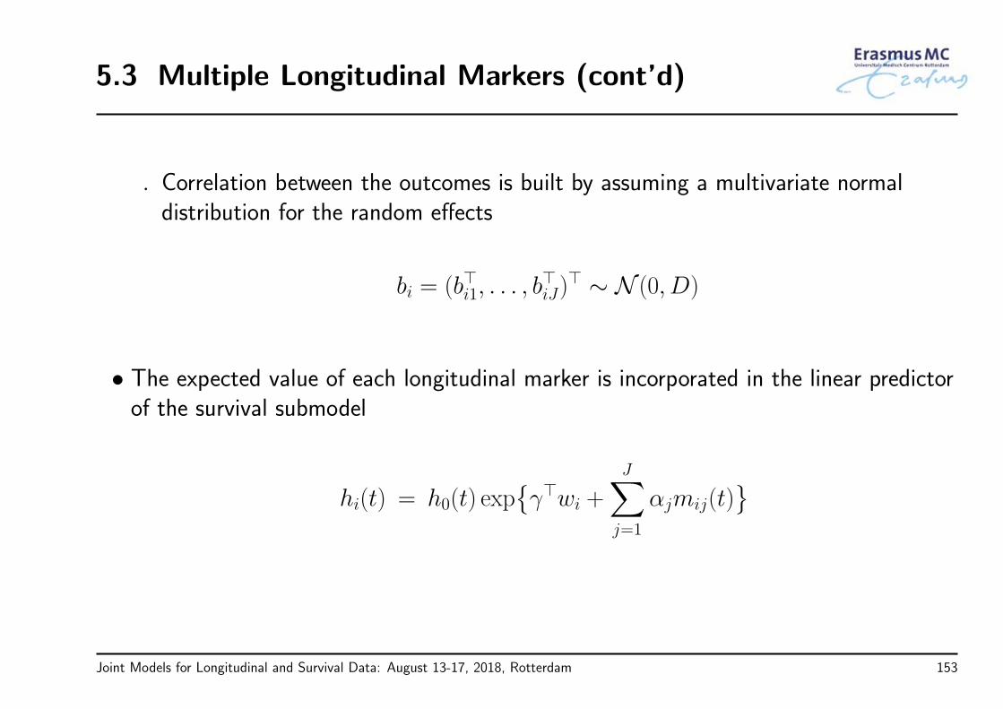
5.3 Multiple Longitudinal Markers (cont’d)
Correlation between the outcomes is built by assuming a multivariate normaldistribution for the random effects
bi = (b⊤i1, . . . , b⊤iJ)
⊤ ∼ N (0, D)
• The expected value of each longitudinal marker is incorporated in the linear predictorof the survival submodel
hi(t) = h0(t) expγ⊤wi +
J∑j=1
αjmij(t)
Joint Models for Longitudinal and Survival Data: August 13-17, 2018, Rotterdam 153
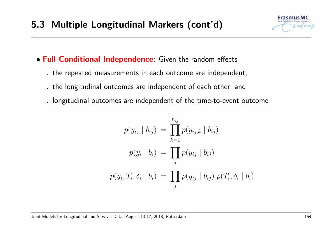
5.3 Multiple Longitudinal Markers (cont’d)
• Full Conditional Independence: Given the random effects
the repeated measurements in each outcome are independent,
the longitudinal outcomes are independent of each other, and
longitudinal outcomes are independent of the time-to-event outcome
p(yij | bij) =
nij∏k=1
p(yij,k | bij)
p(yi | bi) =∏j
p(yij | bij)
p(yi, Ti, δi | bi) =∏j
p(yij | bij) p(Ti, δi | bi)
Joint Models for Longitudinal and Survival Data: August 13-17, 2018, Rotterdam 154

5.3 Multiple Longitudinal Markers (cont’d)
• Features of multivariate joint models
using CI is straightforward to extend joint models to multiple longitudinaloutcomes of different types
computationally much more intensive due to requirement for high dimensionalnumerical integrations with respect to the random effects
Joint Models for Longitudinal and Survival Data: August 13-17, 2018, Rotterdam 155
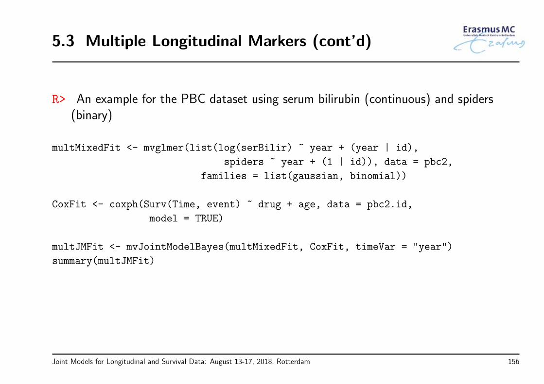
5.3 Multiple Longitudinal Markers (cont’d)
R> An example for the PBC dataset using serum bilirubin (continuous) and spiders(binary)
multMixedFit <- mvglmer(list(log(serBilir) ~ year + (year | id),
spiders ~ year + (1 | id)), data = pbc2,
families = list(gaussian, binomial))
CoxFit <- coxph(Surv(Time, event) ~ drug + age, data = pbc2.id,
model = TRUE)
multJMFit <- mvJointModelBayes(multMixedFit, CoxFit, timeVar = "year")
summary(multJMFit)
Joint Models for Longitudinal and Survival Data: August 13-17, 2018, Rotterdam 156

5.3 Multiple Longitudinal Markers (cont’d)
R> Function mvJointModelBayes() also allows for
right, left, interval censored data
left truncated data
exogenous time-varying covariates
More info and vignettes inhttp://www.drizopoulos.com/ → Software
Joint Models for Longitudinal and Survival Data: August 13-17, 2018, Rotterdam 157

5.4 Multiple Failure Times
• Often multiple failure times are recorded
competing risks
recurrent events
• Example: In the PBC dataset ⇒ competing risks
Some patients received a liver transplantation
So far we have used the composite event, i.e. death or transplantation whatevercomes first
When interest only is on one type of event, the other should be considered as acompeting risk
Joint Models for Longitudinal and Survival Data: August 13-17, 2018, Rotterdam 158

5.4 Multiple Failure Times (cont’d)
• Joint models with competing risks:
yi(t) = mi(t) + εi(t) = x⊤i (t)β + z⊤i (t)bi + εi(t),
hdi (t) = hd0(t) expγ⊤d wi + αdmi(t),
htri (t) = htr0 (t) expγ⊤trwi + αtrmi(t),
where
hdi (t) hazard function for death
htri (t) hazard function for transplantation
Joint Models for Longitudinal and Survival Data: August 13-17, 2018, Rotterdam 159

5.4 Multiple Failure Times (cont’d)
• In the estimation, the only difference is in the construction of the likelihood part forthe event process
p(Ti, δi | bi; θ) =
K∏k=1
[h0k(Ti) expγ⊤k wi + αkmi(Ti)
]I(δi=k)× exp
(−
K∑k=1
∫ Ti
0
h0k(s) expγ⊤k wi + αkmi(s)
ds
),
with
Ti = min(T ∗i1, . . . , T
∗iK, Ci), with Ci denoting the censoring time
δi ∈ 0, 1, . . . , K, with 0 corresponding to censoring
Joint Models for Longitudinal and Survival Data: August 13-17, 2018, Rotterdam 160

5.4 Multiple Failure Times (cont’d)
• This is different than in standard Cox models
i.e., we cannot fit a cause-specific hazard joint model by treating events fromother causes as censored
Joint Models for Longitudinal and Survival Data: August 13-17, 2018, Rotterdam 161
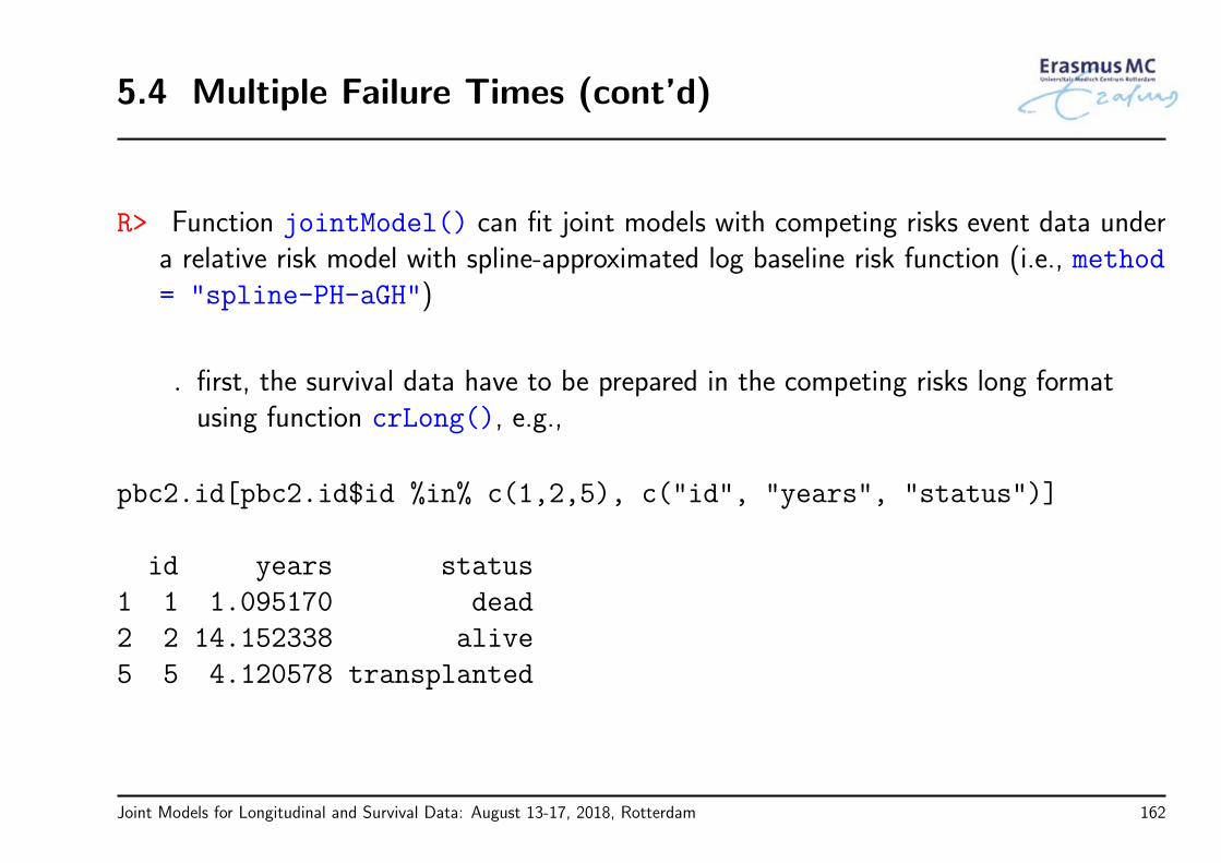
5.4 Multiple Failure Times (cont’d)
R> Function jointModel() can fit joint models with competing risks event data undera relative risk model with spline-approximated log baseline risk function (i.e., method= "spline-PH-aGH")
first, the survival data have to be prepared in the competing risks long formatusing function crLong(), e.g.,
pbc2.id[pbc2.id$id %in% c(1,2,5), c("id", "years", "status")]
id years status
1 1 1.095170 dead
2 2 14.152338 alive
5 5 4.120578 transplanted
Joint Models for Longitudinal and Survival Data: August 13-17, 2018, Rotterdam 162
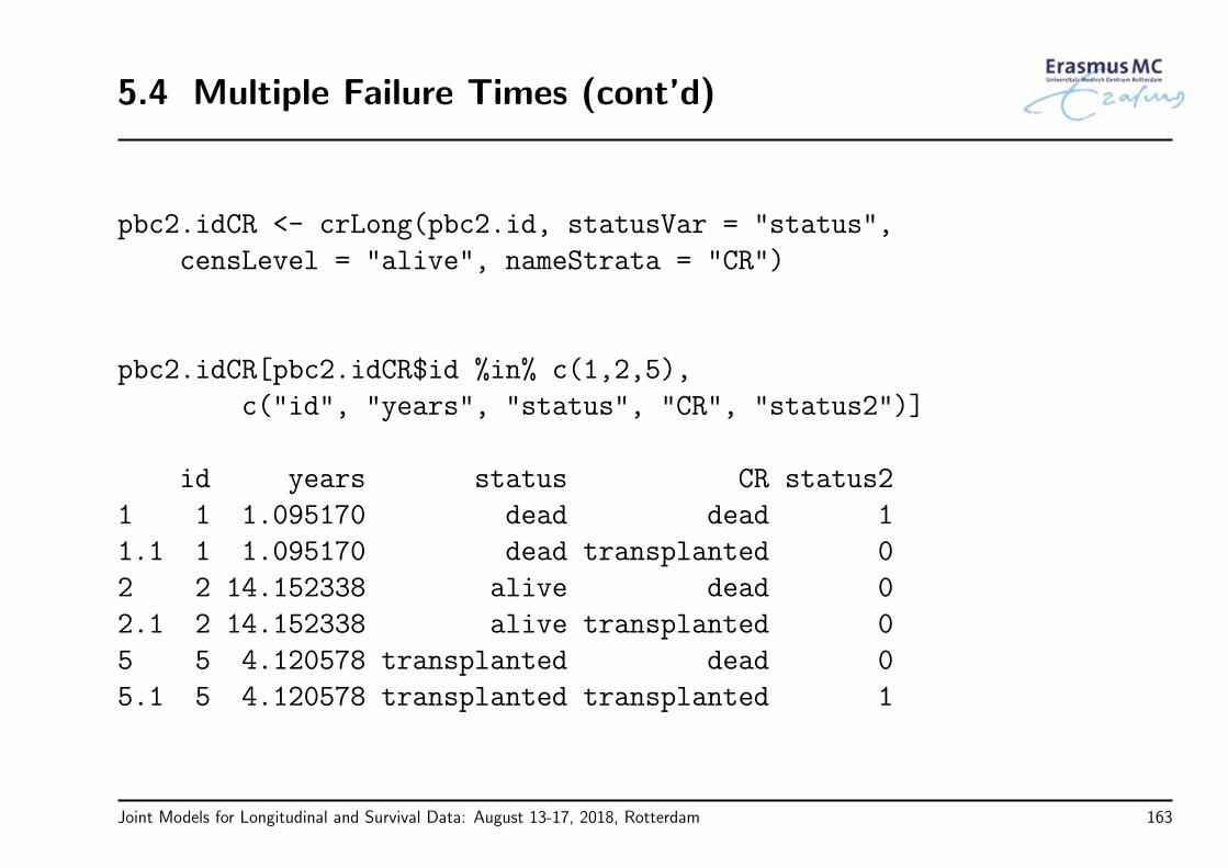
5.4 Multiple Failure Times (cont’d)
pbc2.idCR <- crLong(pbc2.id, statusVar = "status",
censLevel = "alive", nameStrata = "CR")
pbc2.idCR[pbc2.idCR$id %in% c(1,2,5),
c("id", "years", "status", "CR", "status2")]
id years status CR status2
1 1 1.095170 dead dead 1
1.1 1 1.095170 dead transplanted 0
2 2 14.152338 alive dead 0
2.1 2 14.152338 alive transplanted 0
5 5 4.120578 transplanted dead 0
5.1 5 4.120578 transplanted transplanted 1
Joint Models for Longitudinal and Survival Data: August 13-17, 2018, Rotterdam 163

5.4 Multiple Failure Times (cont’d)
R> To fit the joint model, we first fit the linear mixed and relative risk models as before
for the latter we use the data in the competing risks long and put the event-typevariable as strata
lmeFit.CR <- lme(log(serBilir) ~ drug * year, data = pbc2,
random = ~ year | id)
coxFit.CR <- coxph(Surv(years, status2) ~ drug * strata(CR),
data = pbc2.idCR, x = TRUE)
(you can ignore the Warning message)
Joint Models for Longitudinal and Survival Data: August 13-17, 2018, Rotterdam 164

5.4 Multiple Failure Times (cont’d)
R> Then the joint model is fitted with the code
jointFit.CR <- jointModel(lmeFit.CR, coxFit.CR, timeVar = "year",
method = "spline-PH-aGH", CompRisk = TRUE,
interFact = list(value = ~ CR, data = pbc2.idCR))
summary(jointFit.CR)
Joint Models for Longitudinal and Survival Data: August 13-17, 2018, Rotterdam 165

5.4 Multiple Failure Times (cont’d)
• Multiple Failure Times: recurrent events
• Example: In the PBC dataset ⇒ recurrent events
Patients showed irregular visiting patterns
So far, when we fitted the joint model we assumed that the visiting process isnon-informative
If this assumption is violated, we should also model this process in order to obtainvalid inferences
Joint Models for Longitudinal and Survival Data: August 13-17, 2018, Rotterdam 166

5.4 Multiple Failure Times (cont’d)
• Joint model with recurrent (visiting process) & terminal events
yi(t) = mi(t) + εi(t) = x⊤i (t)β + z⊤i (t)bi + εi(t),
ri(t) = r0(t) expγ⊤r wri + αrmi(t) + vi
,
hi(t) = h0(t) expγ⊤h whi + αhmi(t) + ζvi
,
with
ri(t) hazard function for the recurrent events
hi(t) hazard function for the terminal event
vi frailty term accounting for the correlation in the recurrent events
Joint Models for Longitudinal and Survival Data: August 13-17, 2018, Rotterdam 167

5.4 Multiple Failure Times (cont’d)
• Conditional independence assumptions augmented
recurrent events are independent given vi
longitudinal measurements are independent giver bi
all three processes, namely
* longitudinal process,
* recurrent events process, and
* terminating event process
are independent given bi, vi
• We need to postulate a distribution for the frailty terms
typical choice is the Gamma because it’s conjugate
Joint Models for Longitudinal and Survival Data: August 13-17, 2018, Rotterdam 168

5.5 Time-Dependent AFT Models
• Relative risk models most widely used, but
not always most appropriate assumption
does not model expected failure time
• An alternative modeling framework:
Accelerated Failure Time (AFT) model
Joint Models for Longitudinal and Survival Data: August 13-17, 2018, Rotterdam 169

5.5 Time-Dependent AFT Models (cont’d)
• When we only have baseline covariates, the AFT model is the extension of linearregression to survival data, where
we model the expected value of log failure time
we account for censoring in the estimation (no OLS)
log T ∗i = γ⊤wi + ϵi,
where
γ quantifies whether the survival time accelerates or decelerates for every unitchange in the covariate values
the error terms ϵi can be modeled either parametrically or non-parametrically
Joint Models for Longitudinal and Survival Data: August 13-17, 2018, Rotterdam 170

5.5 Time-Dependent AFT Models (cont’d)
• Following the basic idea behind AFT models, Cox and Oakes (1984) proposed thefollowing extension for time-dependent covariates
∫ T ∗
0
expγ⊤w + αm(s)
ds∼ S0,
where S0 denotes the baseline survival function
• With this transformation, and letting
Vi(t) =
∫ t
0
expγ⊤wi + αmi(s)
ds
Joint Models for Longitudinal and Survival Data: August 13-17, 2018, Rotterdam 171

5.5 Time-Dependent AFT Models (cont’d)
• We observe that the survival function of a subject with covariate history Mi(t) takesthe form
Si(t | Mi(t)
)= S0
(Vi(t)
)which means that this subject ages on an accelerated schedule Vi(t) compared to S0
• We also can re-express the time-dependent AFT in terms of the risk rate function
hi(t | Mi(t), wi) = h0(Vi(t)
)expγ⊤wi + αmi(t)
Joint Models for Longitudinal and Survival Data: August 13-17, 2018, Rotterdam 172
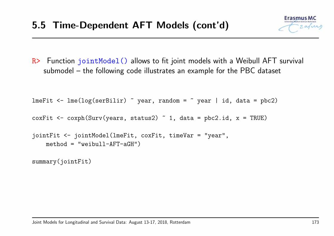
5.5 Time-Dependent AFT Models (cont’d)
R> Function jointModel() allows to fit joint models with a Weibull AFT survivalsubmodel – the following code illustrates an example for the PBC dataset
lmeFit <- lme(log(serBilir) ~ year, random = ~ year | id, data = pbc2)
coxFit <- coxph(Surv(years, status2) ~ 1, data = pbc2.id, x = TRUE)
jointFit <- jointModel(lmeFit, coxFit, timeVar = "year",
method = "weibull-AFT-aGH")
summary(jointFit)
Joint Models for Longitudinal and Survival Data: August 13-17, 2018, Rotterdam 173

5.6 Extensions & Parameterizations
• Note: In the previous extensions of joint models, i.e.,
multiple longitudinal markers
multiple failure times
we used the default parameterization that includes the current value term mi(t) inthe linear predictor of the survival submodel(s)
Nonetheless, all the other parameterizations we have seenearlier are also applicable
Joint Models for Longitudinal and Survival Data: August 13-17, 2018, Rotterdam 174

5.6 Extensions & Parameterizations (cont’d)
• For example in the case of multiple longitudinal outcomes
gj[Eyij(t) | bij
]= mij(t) = x⊤ij(t)βj + z⊤ij(t)bij
hi(t) = h0(t) expγ⊤wi +
J∑j=1
L∑l=1
fjl(Hij(t), αjl)
Joint Models for Longitudinal and Survival Data: August 13-17, 2018, Rotterdam 175

5.6 Extensions & Parameterizations (cont’d)
• In this case we face a challenging model selection problem
• Different possible solutions
lasso
ridge
horseshoe
...
Joint Models for Longitudinal and Survival Data: August 13-17, 2018, Rotterdam 176
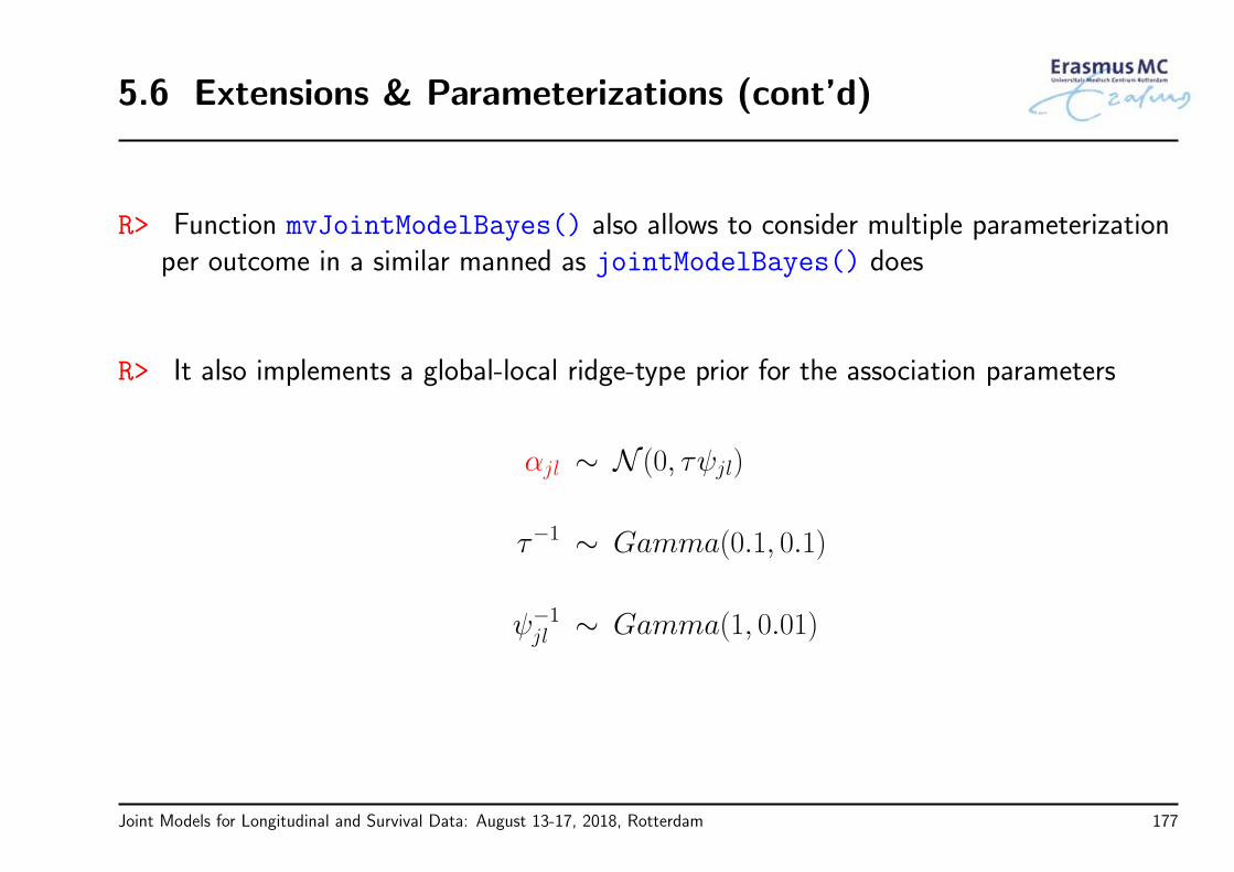
5.6 Extensions & Parameterizations (cont’d)
R> Function mvJointModelBayes() also allows to consider multiple parameterizationper outcome in a similar manned as jointModelBayes() does
R> It also implements a global-local ridge-type prior for the association parameters
αjl ∼ N (0, τψjl)
τ−1 ∼ Gamma(0.1, 0.1)
ψ−1jl ∼ Gamma(1, 0.01)
Joint Models for Longitudinal and Survival Data: August 13-17, 2018, Rotterdam 177

Part VI
Dynamic Predictions, Discrimination & Calibration
Joint Models for Longitudinal and Survival Data: August 13-17, 2018, Rotterdam 178

6.1 Survival Probabilities: Definitions
• Nowadays there is great interest for prognostic models and their application topersonalized medicine
• Examples are numerous
cancer research, cardiovascular diseases, HIV research, . . .
Physicians are interested in accurate prognostic tools that willinform them about the future prospect of a patient in order to
adjust medical care
Joint Models for Longitudinal and Survival Data: August 13-17, 2018, Rotterdam 179

6.1 Survival Probabilities: Definitions (cont’d)
• We are interested in predicting survival probabilities for a new patient j that hasprovided a set of serum bilirubin measurements up to a specific time point t
• Example: We consider Patients 2 and 25 from the PBC dataset that have providedus with 9 and 12 serum bilirubin measurements, respectively
Dynamic Prediction survival probabilities are dynamically updated as additionallongitudinal information is recorded
• We need to account for the endogenous nature of the marker
providing measurements up to time point t ⇒ the patient was still alive at time t
Joint Models for Longitudinal and Survival Data: August 13-17, 2018, Rotterdam 180

6.1 Survival Probabilities: Definitions (cont’d)
Time
log
seru
m b
iliru
bin
−1.0
−0.5
0.0
0.5
1.0
1.5
0 2 4 6 8 10
Patient 2
0 2 4 6 8 10
Patient 25
Joint Models for Longitudinal and Survival Data: August 13-17, 2018, Rotterdam 181

6.1 Survival Probabilities: Definitions (cont’d)
• More formally, for a new subject j we have available measurements up to time point t
Yj(t) = yj(s), 0 ≤ s ≤ t
and we are interested in
πj(u | t) = PrT ∗j ≥ u | T ∗
j > t,Yj(t),Dn
,
where
where u > t, and
Dn denotes the sample on which the joint model was fitted
Joint Models for Longitudinal and Survival Data: August 13-17, 2018, Rotterdam 182
6.2 Survival Probabilities: Estimation
• We assume that the joint model has been fitted to the data at hand
• Based on the fitted model we can estimate the conditional survival probabilities(Rizopoulos, 2011, Biometrics)
Joint Models for Longitudinal and Survival Data: August 13-17, 2018, Rotterdam 183

6.2 Survival Probabilities: Estimation (cont’d)
• πj(u | t) can be rewritten as
πj(u | t) =
∫Sju | Mj(u, bj, θ); θ
Sjt | Mj(t, bj, θ); θ
p(bj | T ∗j > t,Yj(t); θ) dbj
• A naive estimator for πj(u | t) can be constructed by plugging-in the MLEs and theEmpirical Bayes estimates
πj(u | t) =Sju | Mj(u, bj, θ); θ
Sjt | Mj(t, bj, θ); θ
this works relatively well in practice, but
standard errors are difficult to compute
Joint Models for Longitudinal and Survival Data: August 13-17, 2018, Rotterdam 184

6.2 Survival Probabilities: Estimation (cont’d)
• It is convenient to proceed using a Bayesian formulation of the problem ⇒πj(u | t) can be written as
PrT ∗j ≥ u | T ∗
j > t,Yj(t),Dn
=
∫PrT ∗j ≥ u | T ∗
j > t,Yj(t); θp(θ | Dn) dθ
• We have already seen the first part of the integrand
PrT ∗j ≥ u | T ∗
j > t,Yj(t); θ=
=
∫Sju | Mj(u, bj, θ); θ
Sjt | Mj(t, bj, θ); θ
p(bj | T ∗j > t,Yj(t); θ) dbj
Joint Models for Longitudinal and Survival Data: August 13-17, 2018, Rotterdam 185

6.2 Survival Probabilities: Estimation (cont’d)
• Provided that the sample size is sufficiently large, we can approximate the posteriorof the parameters by
θ | Dn ∼ N (θ, H),
where
θ are the MLEs, and
H their asymptotic covariance matrix
Joint Models for Longitudinal and Survival Data: August 13-17, 2018, Rotterdam 186

6.2 Survival Probabilities: Estimation (cont’d)
• A Monte Carlo estimate of πj(u | t) can be obtained using the following simulationscheme:
Step 1. draw θ(ℓ) ∼ N (θ, H)
Step 2. draw b(ℓ)j ∼ bj | T ∗
j > t,Yj(t), θ(ℓ)
Step 3. compute π(ℓ)j (u | t) = Sj
u | Mj(u, b
(ℓ)j , θ
(ℓ)); θ(ℓ)/
Sjt | Mj(t, b
(ℓ)j , θ
(ℓ)); θ(ℓ)
• Repeat Steps 1–3, ℓ = 1, . . . , L times, where L denotes the number of Monte Carlosamples
Joint Models for Longitudinal and Survival Data: August 13-17, 2018, Rotterdam 187

6.2 Survival Probabilities: Estimation (cont’d)
• Steps 1 and 3 are straightforward
• In Step 2 we need to sample from bj | T ∗j > t,Yj(t), θ(ℓ), which is nonstandard
as ni increases, this posterior converges to a multivariate normal distribution(Rizopoulos et al., Biometrika, 2008)
we use a Metropolis-Hastings algorithm with multivariate t proposals
Joint Models for Longitudinal and Survival Data: August 13-17, 2018, Rotterdam 188
6.2 Survival Probabilities: Estimation (cont’d)
• Example: Dynamic predictions of survival probabilities for Patients 2 & 25 from thePBC dataset: We fit the joint model
• Longitudinal submodel
fixed effects: Linear & quadratic time, treatment and their interaction
random effects: Intercept, linear & quadratic time effects
• Survival submodel
treatment effect + underlying serum bilirubin level
piecewise-constant baseline hazard in 7 intervals
Joint Models for Longitudinal and Survival Data: August 13-17, 2018, Rotterdam 189

6.2 Survival Probabilities: Estimation (cont’d)
• Based on the fitted joint model we estimate πj(u | t) for Patients 2 and 25
• We use 500 Monte Carlo samples, and we took as estimate
πj(u | t) = medianπ(ℓ)j (u | t), ℓ = 1, . . . , L
and calculated a corresponding 95% pointwise CIs
Joint Models for Longitudinal and Survival Data: August 13-17, 2018, Rotterdam 190
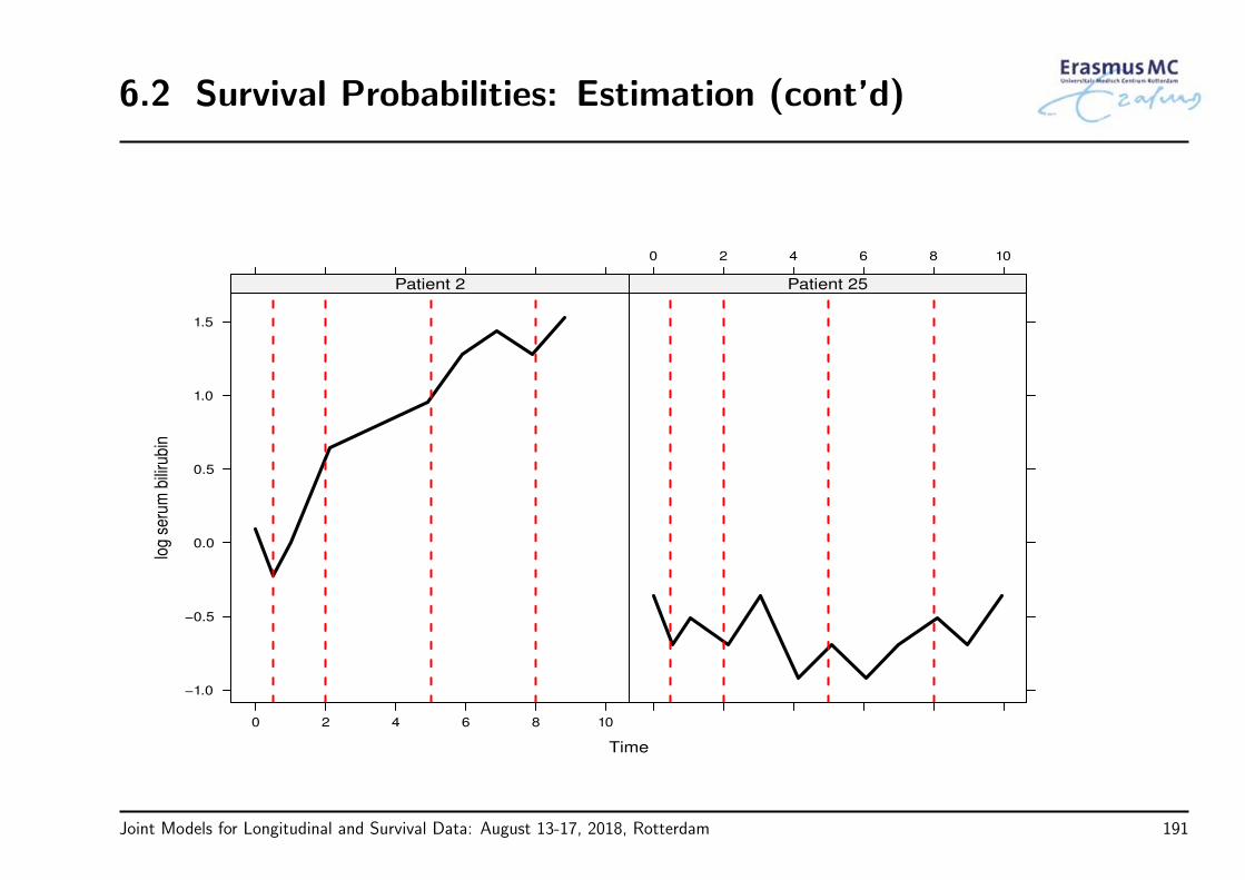
6.2 Survival Probabilities: Estimation (cont’d)
Time
log
seru
m b
iliru
bin
−1.0
−0.5
0.0
0.5
1.0
1.5
0 2 4 6 8 10
Patient 2
0 2 4 6 8 10
Patient 25
Joint Models for Longitudinal and Survival Data: August 13-17, 2018, Rotterdam 191
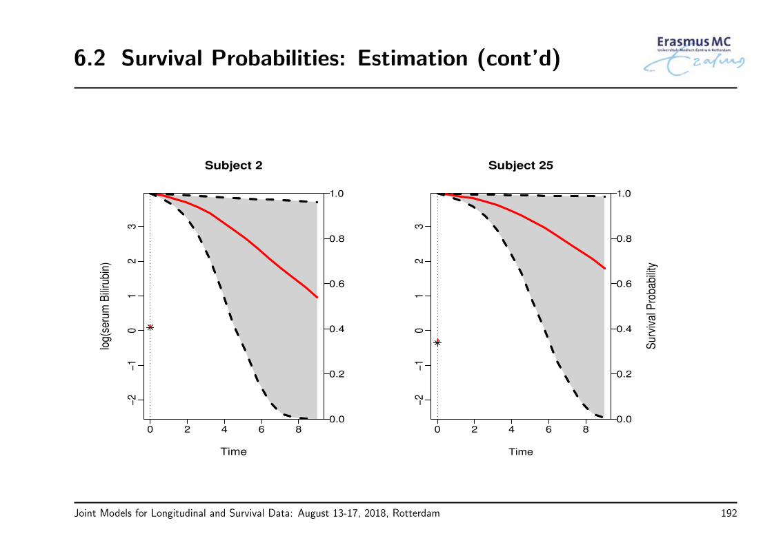
6.2 Survival Probabilities: Estimation (cont’d)
0 2 4 6 8
−2
−1
01
23
Time
log(
seru
m B
iliru
bin)
Subject 2
0.0
0.2
0.4
0.6
0.8
1.0
0 2 4 6 8−
2−
10
12
3
Time
Subject 25
0.0
0.2
0.4
0.6
0.8
1.0
Sur
viva
l Pro
babi
lity
Joint Models for Longitudinal and Survival Data: August 13-17, 2018, Rotterdam 192
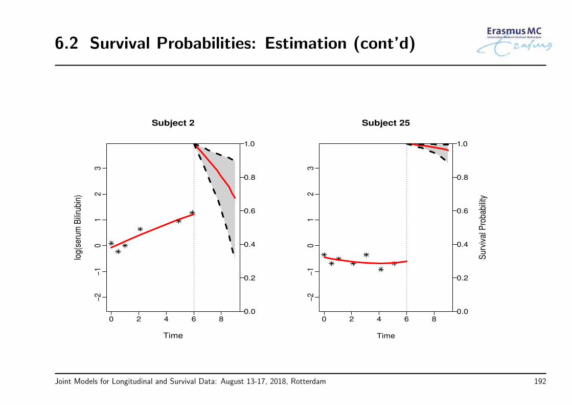

6.2 Survival Probabilities: Estimation (cont’d)
R> Individualized predictions of survival probabilities are computed by functionsurvfitJM() – for example, for Patient 2 from the PBC dataset we have
sfit <- survfitJM(jointFit, newdata = pbc2[pbc2$id == "2", ])
sfit
plot(sfit)
plot(sfit, include.y = TRUE)
Joint Models for Longitudinal and Survival Data: August 13-17, 2018, Rotterdam 193
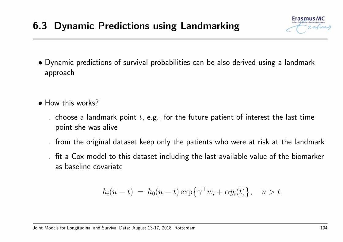
6.3 Dynamic Predictions using Landmarking
• Dynamic predictions of survival probabilities can be also derived using a landmarkapproach
• How this works?
choose a landmark point t, e.g., for the future patient of interest the last timepoint she was alive
from the original dataset keep only the patients who were at risk at the landmark
fit a Cox model to this dataset including the last available value of the biomarkeras baseline covariate
hi(u− t) = h0(u− t) expγ⊤wi + αyi(t)
, u > t
Joint Models for Longitudinal and Survival Data: August 13-17, 2018, Rotterdam 194
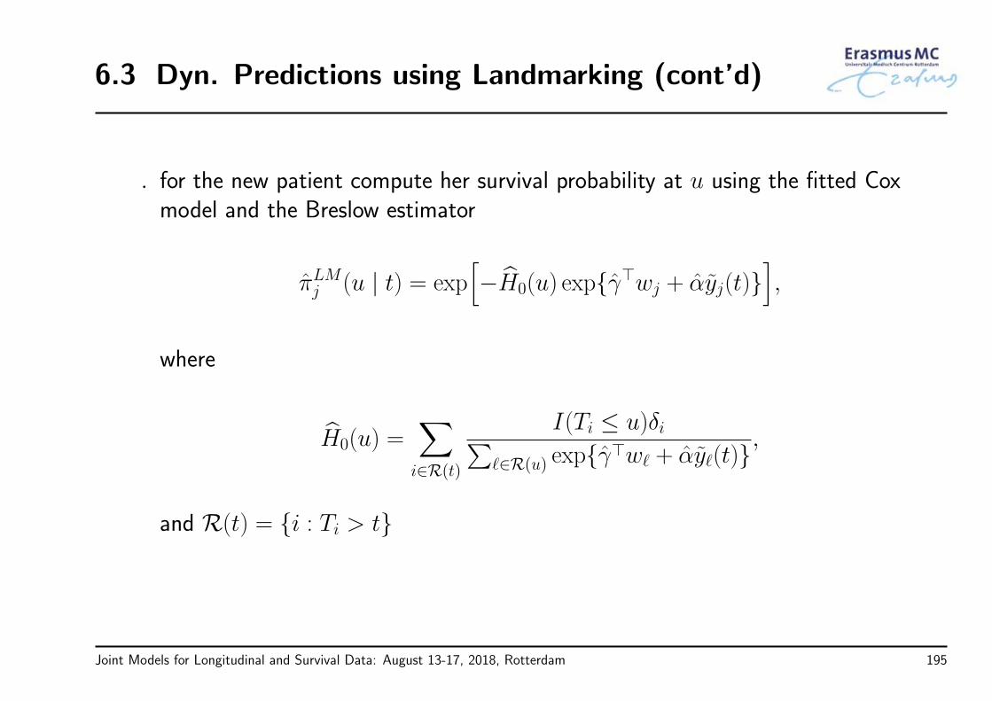
6.3 Dyn. Predictions using Landmarking (cont’d)
for the new patient compute her survival probability at u using the fitted Coxmodel and the Breslow estimator
πLMj (u | t) = exp[−H0(u) expγ⊤wj + αyj(t)
],
where
H0(u) =∑i∈R(t)
I(Ti ≤ u)δi∑ℓ∈R(u) expγ⊤wℓ + αyℓ(t)
,
and R(t) = i : Ti > t
Joint Models for Longitudinal and Survival Data: August 13-17, 2018, Rotterdam 195
6.3 Dyn. Predictions using Landmarking (cont’d)
• Sometimes landmarking works, but not always!
• Main differences between landmarking and joint modeling
Extrapolation:
* both require the level of the marker at t
* landmarking extrapolates the last biomarker value (Last Value Carried Forwardapproach)
* joint modeling builds the subject-specific profile which extrapolates up to t
* from a biological point of view the joint modeling approach seems more logicalthan landmarking
Joint Models for Longitudinal and Survival Data: August 13-17, 2018, Rotterdam 196

6.3 Dyn. Predictions using Landmarking (cont’d)
0 5 10
−2
−1
01
23
Time (years)
Long
itudi
nal O
utco
me
0.0
0.2
0.4
0.6
0.8
1.0
Sur
viva
l Pro
babi
lity
Joint Models for Longitudinal and Survival Data: August 13-17, 2018, Rotterdam 196

6.3 Dyn. Predictions using Landmarking (cont’d)
• Main differences between landmarking and joint modeling
Implicit processes:
Landmarking Joint Modeling* MCAR missing data long. process * MAR missing data long. process
* non-informative visiting process * visiting process allowed to depend onlong. history
* non-informative censoring * censoring allowed to depend onlong. history
Joint Models for Longitudinal and Survival Data: August 13-17, 2018, Rotterdam 197

6.4 Longitudinal Responses: Definitions
• In some occasions it may be also of interest to predict the longitudinal outcome
• We can proceed in the same manner as for the survival probabilities: We haveavailable measurements up to time point t
Yj(t) = yj(s), 0 ≤ s ≤ t
and we are interested in
ωj(u | t) = Eyj(u) | T ∗
j > t,Yj(t),Dn
, u > t
Joint Models for Longitudinal and Survival Data: August 13-17, 2018, Rotterdam 198
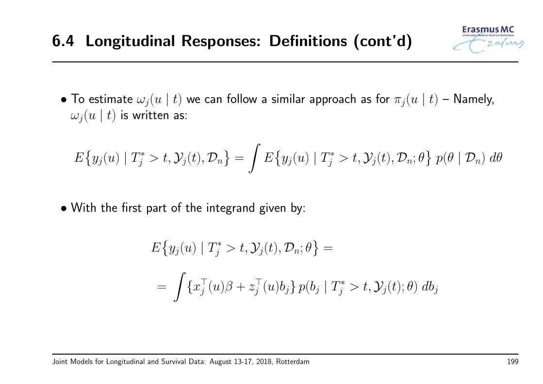
6.4 Longitudinal Responses: Definitions (cont’d)
• To estimate ωj(u | t) we can follow a similar approach as for πj(u | t) – Namely,ωj(u | t) is written as:
Eyj(u) | T ∗
j > t,Yj(t),Dn
=
∫Eyj(u) | T ∗
j > t,Yj(t),Dn; θp(θ | Dn) dθ
• With the first part of the integrand given by:
Eyj(u) | T ∗
j > t,Yj(t),Dn; θ=
=
∫x⊤j (u)β + z⊤j (u)bj p(bj | T ∗
j > t,Yj(t); θ) dbj
Joint Models for Longitudinal and Survival Data: August 13-17, 2018, Rotterdam 199

6.4 Longitudinal Responses: Estimation (cont’d)
• A similar Monte Carlo simulation scheme:
Step 1. draw θ(ℓ) ∼ N (θ, H)
Step 2. draw b(ℓ)j ∼ bj | T ∗
j > t,Yj(t), θ(ℓ)
Step 3. compute ω(ℓ)j (u | t) = x⊤j (u)β
(ℓ) + z⊤j (u)b(ℓ)j
• Note: Prediction intervals can be easily computed by replacing Step 3 with a drawfrom:
ω(ℓ)j (u | t) ∼ N
x⊤j (u)β
(ℓ) + z⊤j (u)b(ℓ)j , [σ2](ℓ)
Joint Models for Longitudinal and Survival Data: August 13-17, 2018, Rotterdam 200

6.4 Longitudinal Responses: Estimation (cont’d)
• Example: Dynamic predictions of serum bilirubin for Patients 2 & 25 from the PBCdataset: We fit the joint model
• Longitudinal submodel
fixed effects: Linear & quadratic time, treatment and their interaction
random effects: Intercept, linear & quadratic time effects
• Survival submodel
treatment effect + underlying serum bilirubin level
piecewise-constant baseline hazard in 7 intervals
Joint Models for Longitudinal and Survival Data: August 13-17, 2018, Rotterdam 201

6.4 Longitudinal Responses: Estimation (cont’d)
• Based on the fitted joint model we estimate ωj(u | t) for Patients 2 and 25
• Point estimates
ωj(u | t) = x⊤j (u)β + z⊤j (u)bj,
where β: MLEs & bj: empirical Bayes estimates
• 95% pointwise CIs
simulation scheme: 2.5% and 97.5% percentiles of 500 Monte Carlo samples of
ω(ℓ)j (u | t)
Joint Models for Longitudinal and Survival Data: August 13-17, 2018, Rotterdam 202
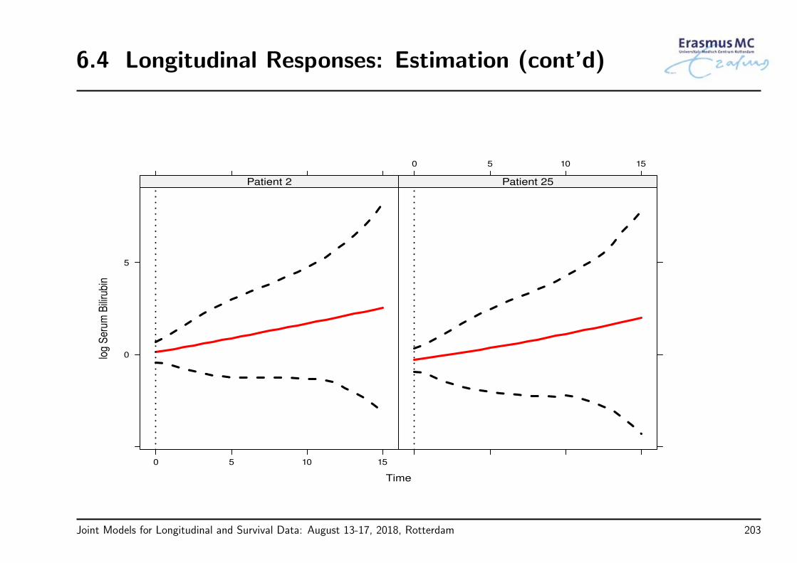
6.4 Longitudinal Responses: Estimation (cont’d)
Time
log
Ser
um B
iliru
bin
0
5
0 5 10 15
Patient 2
0 5 10 15
Patient 25
Joint Models for Longitudinal and Survival Data: August 13-17, 2018, Rotterdam 203

6.4 Longitudinal Responses: Estimation (cont’d)
Time
log
Ser
um B
iliru
bin
−4
−2
0
2
4
6
8
0 5 10 15
Patient 2
0 5 10 15
Patient 25
Joint Models for Longitudinal and Survival Data: August 13-17, 2018, Rotterdam 203

6.4 Longitudinal Responses: Estimation (cont’d)
Time
log
Ser
um B
iliru
bin
−4
−2
0
2
4
6
8
0 5 10 15
Patient 2
0 5 10 15
Patient 25
Joint Models for Longitudinal and Survival Data: August 13-17, 2018, Rotterdam 203
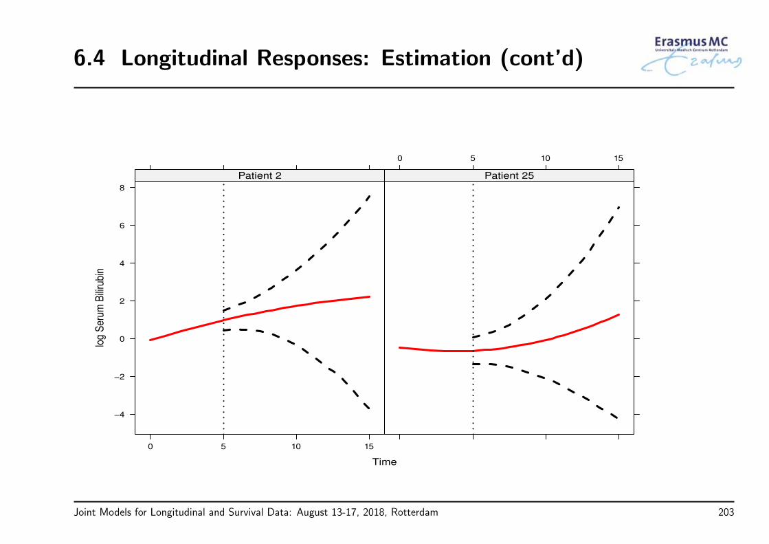
6.4 Longitudinal Responses: Estimation (cont’d)
Time
log
Ser
um B
iliru
bin
−4
−2
0
2
4
6
8
0 5 10 15
Patient 2
0 5 10 15
Patient 25
Joint Models for Longitudinal and Survival Data: August 13-17, 2018, Rotterdam 203

6.4 Longitudinal Responses: Estimation (cont’d)
Time
log
Ser
um B
iliru
bin
−4
−2
0
2
4
6
8
0 5 10 15
Patient 2
0 5 10 15
Patient 25
Joint Models for Longitudinal and Survival Data: August 13-17, 2018, Rotterdam 203
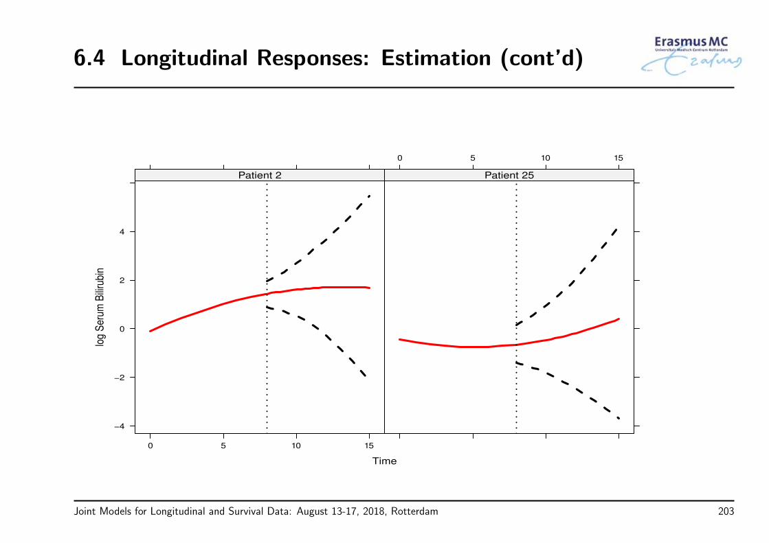
6.4 Longitudinal Responses: Estimation (cont’d)
Time
log
Ser
um B
iliru
bin
−4
−2
0
2
4
0 5 10 15
Patient 2
0 5 10 15
Patient 25
Joint Models for Longitudinal and Survival Data: August 13-17, 2018, Rotterdam 203
6.4 Longitudinal Responses: Estimation (cont’d)
R> Individualized predictions for the longitudinal outcome are computed by functionpredict() – for example, for Patient 2 from the PBC dataset we have function
lfit <- predict(jointFit, newdata = pbc2[pbc2$id == "2", ],
type = "Subject", interval = "conf", returnData = TRUE)
lfit
xyplot(pred + low + upp ~ year, data = lfit, type = "l",
lty = c(1,2,2), col = c(2,1,1), lwd = 2)
Joint Models for Longitudinal and Survival Data: August 13-17, 2018, Rotterdam 204

6.4 Longitudinal Responses: Estimation (cont’d)
R> Web interface using the shiny package
library(shiny)
runApp(file.path(.Library, "JMbayes/demo"))
Joint Models for Longitudinal and Survival Data: August 13-17, 2018, Rotterdam 205

6.5 Importance of the Parameterization
• All previous predictions were based on the standard joint model
hi(t | Mi(t)) = h0(t) expγ⊤wi + αmi(t),
yi(t) = mi(t) + εi(t)
= x⊤i (t)β + z⊤i (t)bi + εi(t),
where Mi(t) = mi(s), 0 ≤ s < t
Joint Models for Longitudinal and Survival Data: August 13-17, 2018, Rotterdam 206

6.5 Importance of the Parameterization (cont’d)
• We have seen earlier that there are several alternative parameterizations (see Section 5.1)
• Relevant questions:
Does the assumed parameterization affect predictions?
Which parameterization is the most optimal?
• Example: We compare predictions for the longitudinal and survival outcomes underdifferent parameterizations for Patient 51 from the PBC study
Joint Models for Longitudinal and Survival Data: August 13-17, 2018, Rotterdam 207
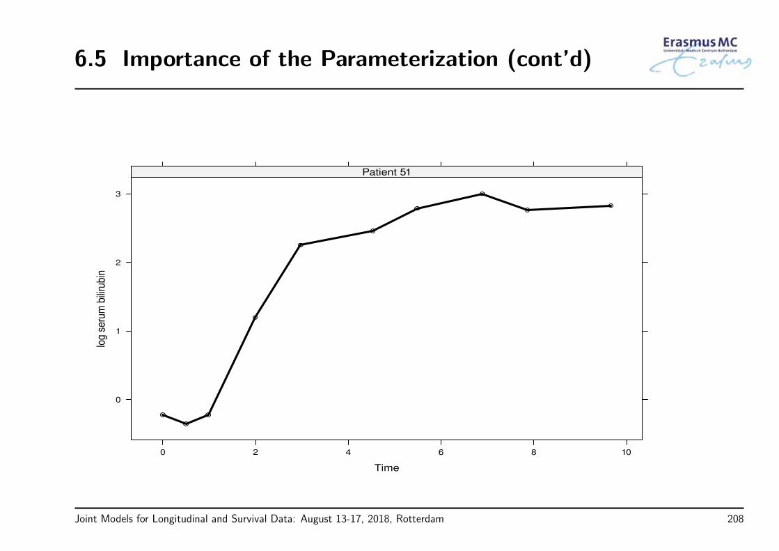
6.5 Importance of the Parameterization (cont’d)
Time
log
seru
m b
iliru
bin
0
1
2
3
0 2 4 6 8 10
Patient 51
Joint Models for Longitudinal and Survival Data: August 13-17, 2018, Rotterdam 208
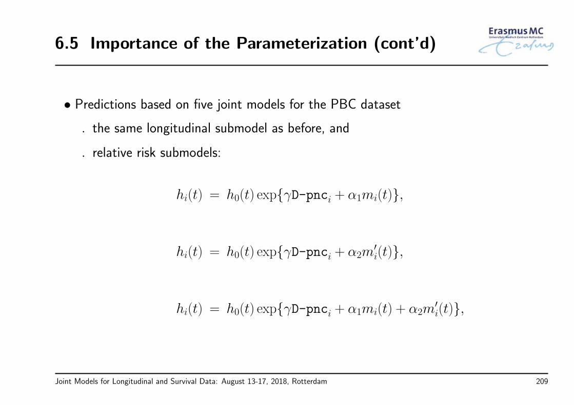
6.5 Importance of the Parameterization (cont’d)
• Predictions based on five joint models for the PBC dataset
the same longitudinal submodel as before, and
relative risk submodels:
hi(t) = h0(t) expγD-pnci + α1mi(t),
hi(t) = h0(t) expγD-pnci + α2m′i(t),
hi(t) = h0(t) expγD-pnci + α1mi(t) + α2m′i(t),
Joint Models for Longitudinal and Survival Data: August 13-17, 2018, Rotterdam 209

6.5 Importance of the Parameterization (cont’d)
hi(t) = h0(t) expγD-pnci + α3
∫ t
0
mi(s)ds,
hi(t) = h0(t) expγD-pnci + α4
∫ t
0
ϕ(t− s)mi(s)ds,
where ϕ(·) standard normal pdf
Joint Models for Longitudinal and Survival Data: August 13-17, 2018, Rotterdam 210

6.5 Importance of the Parameterization (cont’d)
Longitudinal Outcome
Predicted log serum bilirubin
Value
Slope
Value+Slope
Area
weighted Area
u = 1
−1 0 1 2 3 4
u = 1.5 u = 2
−1 0 1 2 3 4
u = 3
Value
Slope
Value+Slope
Area
weighted Area
u = 4 u = 5.5 u = 6.5 u = 7.9
Value
Slope
Value+Slope
Area
weighted Area
−1 0 1 2 3 4
u = 8.9 u = 10.7
Joint Models for Longitudinal and Survival Data: August 13-17, 2018, Rotterdam 211

6.5 Importance of the Parameterization (cont’d)
Survival Outcome
Survival Probability
Value
Slope
Value+Slope
Area
weighted Area
u = 1
0.2 0.4 0.6 0.8 1.0
u = 1.5 u = 2
0.2 0.4 0.6 0.8 1.0
u = 3
Value
Slope
Value+Slope
Area
weighted Area
u = 4 u = 5.5 u = 6.5 u = 7.9
Value
Slope
Value+Slope
Area
weighted Area
0.2 0.4 0.6 0.8 1.0
u = 8.9 u = 10.7
Joint Models for Longitudinal and Survival Data: August 13-17, 2018, Rotterdam 212
6.5 Importance of the Parameterization (cont’d)
• The chosen parameterization can influence the derived predictions
especially for the survival outcome
• My current work: How to optimally choose parameterization?
per subject (personalized medicine)
• Quite promising results from the Bayesian approach using Bayesian Model Averagingtechniques
it can be done with package JMbayes,
it falls a bit outside the scope of this course, but
I can provide information if interested. . .
Joint Models for Longitudinal and Survival Data: August 13-17, 2018, Rotterdam 213
6.6 Marker Discrimination: Definitions
• Often clinical interest lies in the predictive performance of a marker
how good is serum bilirubin in discriminating between patients of low and highrisk of dying
• We develop and estimate prospective accuracy measures based on ROC methodologywithin the joint modeling framework
Joint Models for Longitudinal and Survival Data: August 13-17, 2018, Rotterdam 214

6.6 Marker Discrimination: Definitions (cont’d)
• General setting: For any t, we are interested in events in the medically relevant timeinterval (t, t +∆t] (Heargety & Zheng, Bcs, 2005; Zheng & Heargety, Bcs, 2007)
• In particular,
two generic patients, i and j
have survived up to time t
provided us with a series of marker values,Yi(t) = yi(s), 0 ≤ s ≤ t and Yj(t) = yj(s), 0 ≤ s ≤ t
Patient i died before t +∆t, Patient j lived longer
• Goal: Use the marker to discriminate between these two patients and take anappropriate medical action
Joint Models for Longitudinal and Survival Data: August 13-17, 2018, Rotterdam 215

6.6 Marker Discrimination: Definitions (cont’d)
• General prediction rule: We define “success” as
Si(t, k, c) = yi(s) ≥ cs; k ≤ s ≤ t,
where
yi(s) the value of the marker at time s
c vector of threshold values
k specifies which past values of the marker we are using
• Note: In case lower yi(t) values are more predictive for an event, then
Si(t, k, c) = yi(s) ≤ cs; k ≤ s ≤ t
Joint Models for Longitudinal and Survival Data: August 13-17, 2018, Rotterdam 216

6.6 Marker Discrimination: Definitions (cont’d)
• Examples: Simple/Standard Prediction Rule
Si(t, k = t, c) = yi(t) ≥ c
we use the most recent measurement to guide decision making
Joint Models for Longitudinal and Survival Data: August 13-17, 2018, Rotterdam 217

6.6 Marker Discrimination: Definitions (cont’d)
• Examples: Composite Prediction Rule
Si(t, k = t− 1, c) = yi(t− 1) ≥ c ∪ yi(t) ≥ c
or
Si(t, k = t− 1, c) = yi(t− 1) ≥ c ∪ yi(t) ≥ (1 + v)c
we use the last two measurements
the same threshold or (100× v)% increase from the pre-last to the last one
Joint Models for Longitudinal and Survival Data: August 13-17, 2018, Rotterdam 218

6.6 Marker Discrimination: Definitions (cont’d)
• Sensitivity
TP∆tt = Pr
Si(t, k, c) | T ∗
i > t, T ∗i ∈ (t, t +∆t]
• Specificity
1− FP∆tt = Pr
Fi(t, k, c) | T ∗
i > t, T ∗i > t +∆t
where
T ∗i true failure time
Fi(t, k, c) = Rq \ Si(t, k, c) with q # measurements in [k, t]
Joint Models for Longitudinal and Survival Data: August 13-17, 2018, Rotterdam 219

6.6 Marker Discrimination: Definitions (cont’d)
• Time-dependent ROCs
ROC∆tt (p) = TP∆t
t [FP∆tt ]−1(p)
and AUCs
AUC∆tt =
∫ 1
0
ROC∆tt (p) dp
can be used to assess the performance of the longitudinal marker at specific follow-uptimes
Joint Models for Longitudinal and Survival Data: August 13-17, 2018, Rotterdam 220

6.7 Marker Discrimination: Estimation
• For the estimation of the accuracy measures we need to account for censoring
• We take full advantage of the joint modeling framework
we have estimated the joint distribution T ∗i , yi(t)
conditional independence
Joint Models for Longitudinal and Survival Data: August 13-17, 2018, Rotterdam 221
6.7 Marker Discrimination: Estimation (cont’d)
• Joint model is estimated using maximum likelihood
• Based on the fitted joint model we can estimate the sensitivity and specificity using aMonte Carlo simulation scheme similar to the one used for πi(u | t) technical details skipped–more info available at Rizopoulos (2011, Biometrics)
Joint Models for Longitudinal and Survival Data: August 13-17, 2018, Rotterdam 222
6.7 Marker Discrimination: Estimation (cont’d)
• Example: We calculate time-dependent ROCs for the PBC data – in particular,
two generic patients (one placebo; one D-penicillamine)
providing measurements at t = 0, 0.5, 2, 3, and 5 years
relevant time windows ∆t = 1, 2, and 4 years
2000 Monte Carlo samples
• Prediction rule: Simple (using the most recent bilirubin measurement)
Joint Models for Longitudinal and Survival Data: August 13-17, 2018, Rotterdam 223

6.7 Marker Discrimination: Estimation (cont’d)
0.0 0.2 0.4 0.6 0.8 1.0
0.0
0.2
0.4
0.6
0.8
1.0
Case placebo
1 − Specificity
Sen
sitiv
ity
0.0 0.2 0.4 0.6 0.8 1.0
0.0
0.2
0.4
0.6
0.8
1.0
Case D−penicil
1 − Specificity
Sen
sitiv
ity
Follow−up: 0
∆t = 1
∆t = 2
∆t = 4
Joint Models for Longitudinal and Survival Data: August 13-17, 2018, Rotterdam 224

6.7 Marker Discrimination: Estimation (cont’d)
0.0 0.2 0.4 0.6 0.8 1.0
0.0
0.2
0.4
0.6
0.8
1.0
Case placebo
1 − Specificity
Sen
sitiv
ity
0.0 0.2 0.4 0.6 0.8 1.0
0.0
0.2
0.4
0.6
0.8
1.0
Case D−penicil
1 − Specificity
Sen
sitiv
ity
Follow−up: 0, 0.5
∆t = 1
∆t = 2
∆t = 4
Joint Models for Longitudinal and Survival Data: August 13-17, 2018, Rotterdam 224

6.7 Marker Discrimination: Estimation (cont’d)
0.0 0.2 0.4 0.6 0.8 1.0
0.0
0.2
0.4
0.6
0.8
1.0
Case placebo
1 − Specificity
Sen
sitiv
ity
0.0 0.2 0.4 0.6 0.8 1.0
0.0
0.2
0.4
0.6
0.8
1.0
Case D−penicil
1 − Specificity
Sen
sitiv
ity
Follow−up: 0, 0.5, 2
∆t = 1
∆t = 2
∆t = 4
Joint Models for Longitudinal and Survival Data: August 13-17, 2018, Rotterdam 224

6.7 Marker Discrimination: Estimation (cont’d)
0.0 0.2 0.4 0.6 0.8 1.0
0.0
0.2
0.4
0.6
0.8
1.0
Case placebo
1 − Specificity
Sen
sitiv
ity
0.0 0.2 0.4 0.6 0.8 1.0
0.0
0.2
0.4
0.6
0.8
1.0
Case D−penicil
1 − Specificity
Sen
sitiv
ity
Follow−up: 0, 0.5, 2, 3
∆t = 1
∆t = 2
∆t = 4
Joint Models for Longitudinal and Survival Data: August 13-17, 2018, Rotterdam 224

6.7 Marker Discrimination: Estimation (cont’d)
0.0 0.2 0.4 0.6 0.8 1.0
0.0
0.2
0.4
0.6
0.8
1.0
Case placebo
1 − Specificity
Sen
sitiv
ity
0.0 0.2 0.4 0.6 0.8 1.00.
00.
20.
40.
60.
81.
0
Case D−penicil
1 − Specificity
Sen
sitiv
ity
Follow−up: 0, 0.5, 2, 3, 5
∆t = 1
∆t = 2
∆t = 4
Joint Models for Longitudinal and Survival Data: August 13-17, 2018, Rotterdam 224

6.7 Marker Discrimination: Estimation (cont’d)
R> Time-dependent sensitivity, specificity and ROCs are computed by functionrocJM() – for the PBC dataset example we have
NewData <- expand.grid(
year = c(0, 0.5, 2, 3, 5),
drug = c("placebo", "D-penicil")
)
NewData$id <- rep(1:2, each = 5)
roc <- rocJM(jointFit, data = NewData, dt = c(1, 2, 4))
roc
plot(roc)
Joint Models for Longitudinal and Survival Data: August 13-17, 2018, Rotterdam 225

6.8 Model Discrimination
• In the previous we have concentrated on the discriminative capability of thelongitudinal biomarker
this could be useful in medical practice if the marker alone offers good enoughdiscrimination
• But often we are also interested in the discriminative capability of the whole modelincorporating the baseline covariates as well
especially when no single prognostic factor can accurately enough discriminatebetween patients
Joint Models for Longitudinal and Survival Data: August 13-17, 2018, Rotterdam 226
6.8 Model Discrimination (cont’d)
• We assume a similar setting as before for assessing the discriminative capability of ajoint model
using the available longitudinal data up to time t, Yj(t) = yj(s), 0 ≤ s ≤ t
we are interested in events in the medically relevant interval (t, t +∆t]
• Based on the fitted joint model and for a particular threshold value c ∈ [0, 1], we canterm a subject as a case if
πj(t +∆t | t) ≤ c
Joint Models for Longitudinal and Survival Data: August 13-17, 2018, Rotterdam 227

6.8 Model Discrimination (cont’d)
• Following, we can define sensitivity
Prπj(t +∆t | t) ≤ c | T ∗
j ∈ (t, t +∆t],
specificity
Prπj(t +∆t | t) > c | T ∗
j > t +∆t,
and the corresponding AUC
AUC(t,∆t)
= Pr[πi(t +∆t | t) < πj(t +∆t | t) | T ∗
i ∈ (t, t +∆t] ∩ T ∗j > t +∆t
]
Joint Models for Longitudinal and Survival Data: August 13-17, 2018, Rotterdam 228

6.8 Model Discrimination (cont’d)
• Estimation of AUC(t,∆t) can be based on similar arguments as Harrell’s C index
AUC(t,∆t) = AUC1(t,∆t) + AUC2(t,∆t)
where
AUC1(t,∆t) =
∑ni=1
∑nj=1;j =i Iπi(t +∆t | t) < πj(t +∆t | t) × IΩ(1)
ij (t)∑ni=1
∑nj=1;j =i IΩ
(1)ij (t)
,
with
Ω(1)ij (t) =
[Ti ∈ (t, t +∆t] ∩ δi = 1
]∩ Tj > t +∆t
Joint Models for Longitudinal and Survival Data: August 13-17, 2018, Rotterdam 229

6.8 Model Discrimination (cont’d)
• And
AUC2(t,∆t) =
∑ni=1
∑nj=1;j =i Iπi(t +∆t | t) < πj(t +∆t | t) × IΩ(2)
ij (t) × K∑ni=1
∑nj=1;j =i IΩ
(2)ij (t) × K
,
with
Ω(2)ij (t) =
[Ti ∈ (t, t +∆t] ∩ δi = 0
]∩ Tj > t +∆t
and
K = 1− πi(t +∆t | Ti)
Joint Models for Longitudinal and Survival Data: August 13-17, 2018, Rotterdam 230
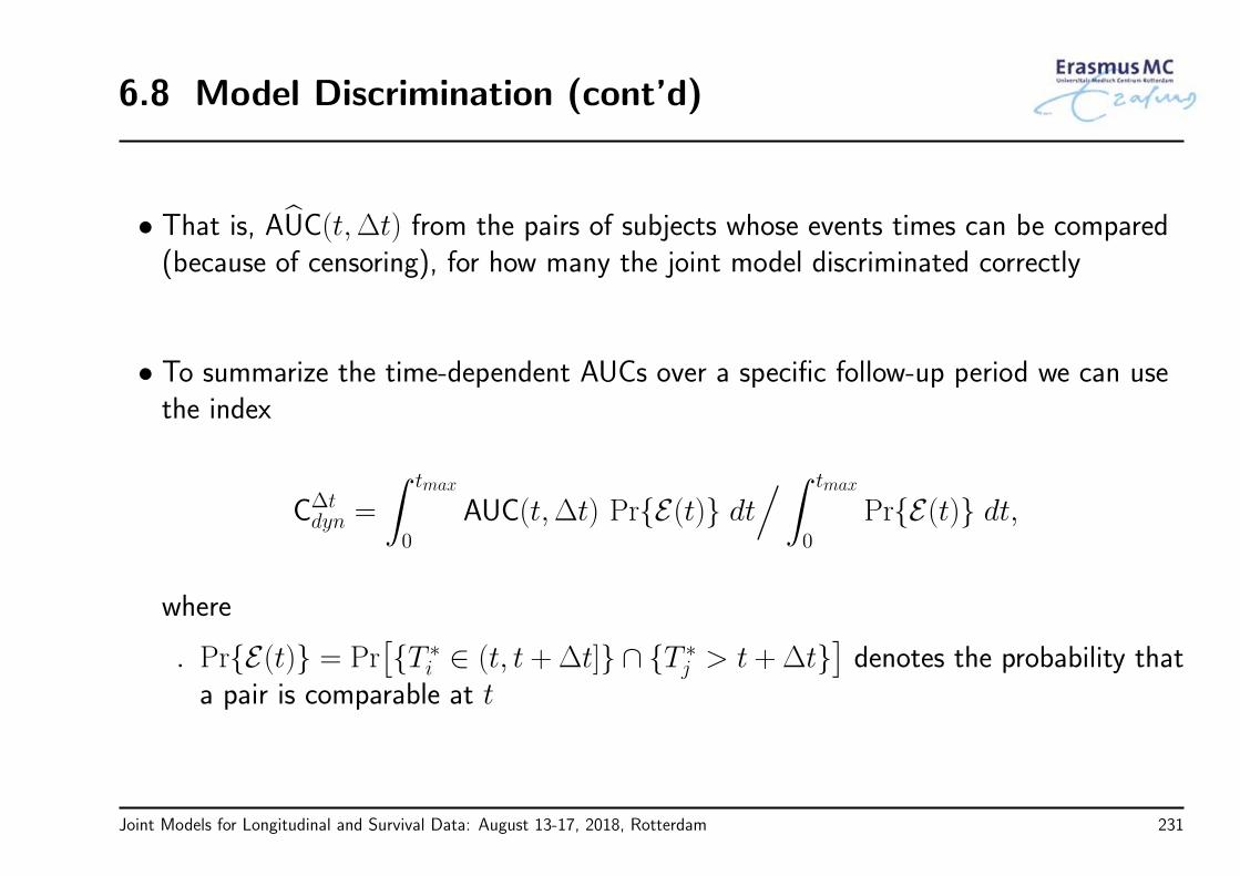
6.8 Model Discrimination (cont’d)
• That is, AUC(t,∆t) from the pairs of subjects whose events times can be compared(because of censoring), for how many the joint model discriminated correctly
• To summarize the time-dependent AUCs over a specific follow-up period we can usethe index
C∆tdyn =
∫ tmax
0
AUC(t,∆t) PrE(t) dt/∫ tmax
0
PrE(t) dt,
where
PrE(t) = Pr[T ∗
i ∈ (t, t+∆t] ∩ T ∗j > t+∆t
]denotes the probability that
a pair is comparable at t
Joint Models for Longitudinal and Survival Data: August 13-17, 2018, Rotterdam 231
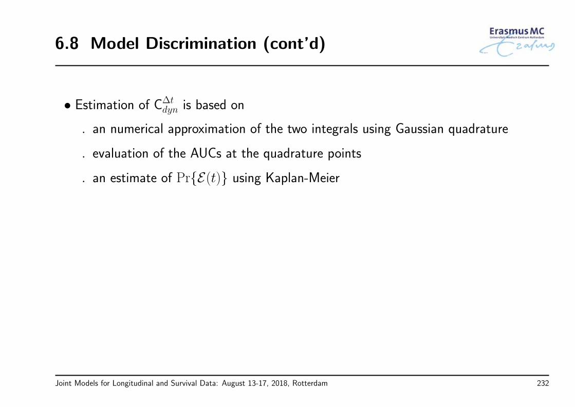
6.8 Model Discrimination (cont’d)
• Estimation of C∆tdyn is based on
an numerical approximation of the two integrals using Gaussian quadrature
evaluation of the AUCs at the quadrature points
an estimate of PrE(t) using Kaplan-Meier
Joint Models for Longitudinal and Survival Data: August 13-17, 2018, Rotterdam 232

6.8 Model Discrimination (cont’d)
R> For a fitted joint model AUC(t,∆t) and C∆t
dyn are calculated by functions aucJM()and dynCJM(), respectively – for the PBC dataset
# AUC(t = 7, Delta t = 2)
aucJM(jointFit, newdata = pbc2, Tstart = 7, Dt = 2)
# C_dyn(Delta t = 2) in the interval [0, 10]
dynCJM(jointFit, newdata = pbc2, Dt = 2, t.max = 10)
Joint Models for Longitudinal and Survival Data: August 13-17, 2018, Rotterdam 233

6.9 Calibration
• We have extensively covered discrimination, i.e.,
how well can the longitudinal biomarker(s) discriminate between subject of lowand high risk for the event
• Another relevant measure for quantifying predictive ability is calibration, i.e.,
how well can the longitudinal biomarker(s) accurately predict future events
• In standard survival analysis and on the latter front there has been a lot of work onextensions of the Brier score (see Gerds and Schumacher, (2006) and references therein)
Joint Models for Longitudinal and Survival Data: August 13-17, 2018, Rotterdam 234

6.9 Calibration (cont’d)
• In the joint modeling framework we need to take into account the dynamic nature ofthe longitudinal marker
• The expected error of prediction has the form
PE(u | t) = E[LNi(u)− πi(u | t)
]where
Ni(t) = I(T ∗i > t) is the event status at time t
L(·) denotes a loss function, such as the absolute or square loss
Joint Models for Longitudinal and Survival Data: August 13-17, 2018, Rotterdam 235
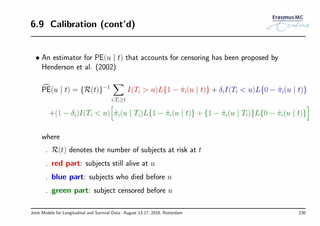
6.9 Calibration (cont’d)
• An estimator for PE(u | t) that accounts for censoring has been proposed byHenderson et al. (2002)
PE(u | t) = R(t)−1∑i:Ti≥t
I(Ti > u)L1− πi(u | t) + δiI(Ti < u)L0− πi(u | t)
+(1− δi)I(Ti < u)[πi(u | Ti)L1− πi(u | t) + 1− πi(u | Ti)L0− πi(u | t)
]where
R(t) denotes the number of subjects at risk at t
red part: subjects still alive at u
blue part: subjects who died before u
green part: subject censored before u
Joint Models for Longitudinal and Survival Data: August 13-17, 2018, Rotterdam 236

6.9 Calibration (cont’d)
• PE(u | t) uses the longitudinal information up to time t and focuses on accuracy atsingle time point u
alternatively, we could summarize the error of prediction in a specific interval ofinterest, say [t, u]
• A weighted average of PE(u | t) that accounts for the reduction in the number ofevents due to censoring:
IPE(u | t) =
∑i:t≤Ti≤u
δiSC(t)/SC(Ti)
PE(u | t)∑
i:t≤Ti≤uδiSC(t)/SC(Ti)
where
SC(·) denotes the Kaplan-Meier estimator of the censoring time distribution
Joint Models for Longitudinal and Survival Data: August 13-17, 2018, Rotterdam 237

6.9 Calibration (cont’d)
• Both IPE(u | t) and PE(u | t) can be used to provide a measure of explainedvariation between nested models
• Say model M1 is nested in model M2, we can compute how much the extra structurein M2 improves accuracy by
R2PE(u | t;M1,M2) = 1− PEM2(u | t)
/PEM1(u | t)
or
R2IPE(u | t;M1,M2) = 1− IPEM2(u | t)
/IPEM1(u | t)
Joint Models for Longitudinal and Survival Data: August 13-17, 2018, Rotterdam 238

6.9 Calibration (cont’d)
R> For a fitted joint model PE(u | t) and IPE(u | t) are calculated by functionprederrJM() – for the PBC dataset
# PE(u = 9 | t = 7)
prederrJM(jointFit, newdata = pbc2, Tstart = 7, Thoriz = 9)
# IPE(u = 9 | t = 7)
prederrJM(jointFit, newdata = pbc2, Tstart = 7, Thoriz = 9,
interval = TRUE)
Joint Models for Longitudinal and Survival Data: August 13-17, 2018, Rotterdam 239

6.10 Landmarking vs JM: An Example
• We have earlier seen that the landmark approach also provides estimates of dynamicsurvival probabilities πj(u | t) we make here a comparison here with joint modeling for the PBC dataset
• Joint models:
Longitudinal process:
yi(t) = β1Plcbi + β2D-penci + β3B1(t, λ)× Plcbi + β4B1(t, λ)× D-penci+ β5B2(t, λ)× Plcbi + β6B2(t, λ)× D-penci+ β7B3(t, λ)× Plcbi + β8B3(t, λ)× D-penci+ bi0 + bi1B1(t, λ) + bi2B2(t, λ) + bi3B3(t, λ) + εi(t),
Joint Models for Longitudinal and Survival Data: August 13-17, 2018, Rotterdam 240

6.10 Landmarking vs JM: An Example (cont’d)
• Joint models:
Survival process:
M1 : hi(t) = h0(t) expγ1D-penci + γ2Agei + γ3Femalei + α1mi(t)
,
M2 : hi(t) = h0(t) expγ1D-penci + γ2Agei + γ3Femalei + α1mi(t) + α2m
′i(t),
M3 : hi(t) = h0(t) expγ1D-penci + γ2Agei + γ3Femalei + α1
∫ t
0
mi(s)ds,
M4 : hi(t) = h0(t) exp(γ1D-penci + γ2Agei + γ3Femalei
+ α1bi0 + α2bi1 + α3bi2 + α4bi3),
Joint Models for Longitudinal and Survival Data: August 13-17, 2018, Rotterdam 241

6.10 Landmarking vs JM: An Example (cont’d)
• We focus on the interval [t = 7, u = 9] and we fit a series of Cox models to thepatients at risk at t = 7 with corresponding association structures to the previousjoint models, i.e.,
M5 : hi(u− 7) = h0(u− 7) expγ1D-penci + γ2Agei + γ3Femalei + α1yi(7)
,
M6 : hi(u− 7) = h0(u− 7) expγ1D-penci + γ2Agei + γ3Femalei+ α1yi(7) + α2y
′i(7),
M7 : hi(u− 7) = h0(u− 7) expγ1D-penci + γ2Agei + γ3Femalei
+ α1
7∑s=0
yi(s)∆s,
Joint Models for Longitudinal and Survival Data: August 13-17, 2018, Rotterdam 242
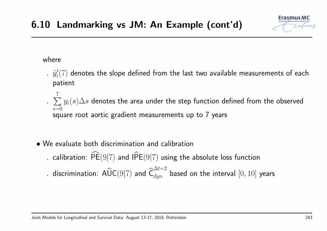
6.10 Landmarking vs JM: An Example (cont’d)
where
y′i(7) denotes the slope defined from the last two available measurements of eachpatient
7∑s=0
yi(s)∆s denotes the area under the step function defined from the observed
square root aortic gradient measurements up to 7 years
• We evaluate both discrimination and calibration
calibration: PE(9|7) and IPE(9|7) using the absolute loss function
discrimination: AUC(9|7) and C∆t=2
dyn based on the interval [0, 10] years
Joint Models for Longitudinal and Survival Data: August 13-17, 2018, Rotterdam 243

6.10 Landmarking vs JM: An Example (cont’d)
PE(9|7) IPE(9|7) AUC(9|7) C∆t=2
dyn
M1: JM value 0.201 0.118 0.787 0.854
M2: JM value+slope 0.197 0.114 0.793 0.855
M3: JM area 0.191 0.112 0.758 0.839
M4: JM shared RE 0.191 0.108 0.807 0.840
M5 : CoxLM value 0.229 0.127 0.702 0.841
M6 : CoxLM value+slope 0.227 0.126 0.710 0.825
M7 : CoxLM area 0.226 0.125 0.697 0.827
• For this particular dataset and comparing the same parameterization we observe thatjoint modeling is better in terms of both calibration and discrimination
Joint Models for Longitudinal and Survival Data: August 13-17, 2018, Rotterdam 244

6.11 Validation
• Validation of both discrimination and calibration measures can be achieved withstandard re-sampling techniques
cross-validation (leave-one-out or better 10-fold)
Bootstrap
• In general time consuming because it requires fitting the joint model many times
take advantage of parallel computing (e.g., using package parallel)
Joint Models for Longitudinal and Survival Data: August 13-17, 2018, Rotterdam 245

Part VII
Closing
Joint Models for Longitudinal and Survival Data: August 13-17, 2018, Rotterdam 246

7.1 Concluding Remarks
• When we need joint models for longitudinal and survival outcomes?
to handle endogenous time-varying covariates in a survival analysis context
to account for nonrandom dropout in a longitudinal data analysis context
• How joint models work?
a mixed model for the longitudinal outcome
a relative risk model for the event process
explain interrelationships with shared random effects
Joint Models for Longitudinal and Survival Data: August 13-17, 2018, Rotterdam 247

7.1 Concluding Remarks (cont’d)
• Where to pay attention when defining joint models?
model flexibly the subject-specific evolutions for the longitudinal outcome
use parametric but flexible models for the baseline hazard function
consider how to model the association structure between the two processes⇒ Parameterization
• Extensions
under the full conditional independence assumption we can easily extend the basicjoint model
multiple longitudinal outcomes and/or multiple failure times
though more computationally intensive
Joint Models for Longitudinal and Survival Data: August 13-17, 2018, Rotterdam 248

7.1 Concluding Remarks (cont’d)
• Individualized predictions
joint models can provide subject-specific predictions for the longitudinal andsurvival outcomes
these are dynamically updated as extra information is recorded for the subjects
⇒ joint models constitute an excellent tool for personalized medicine
• What we did not cover
diagnostics for joint models using residuals
. . .
Joint Models for Longitudinal and Survival Data: August 13-17, 2018, Rotterdam 249

The End!
Joint Models for Longitudinal and Survival Data: August 13-17, 2018, Rotterdam 250

7.2 Additional References
• Andrinopoulou, E.R., Rizopoulos, D., Takkenberg, J. and Lesaffre, E. (2014). Joint modeling of two longitudinaloutcomes and competing risk data. Statistics in Medicine, to appear.
• Brown, E. and Ibrahim, J. (2003). A Bayesian semiparametric joint hierarchical model for longitudinal and survivaldata. Biometrics 59, 221–228.
• Brown, E. Ibrahim, J. and DeGruttola, V. (2005). A flexible B-spline model for multiple longitudinal biomarkers andsurvival. Biometrics 61, 64–73.
• Chi, Y.-Y. and Ibrahim, J. (2006). Joint models for multivariate longitudinal and multivariate survival data.Biometrics 62, 432–445.
• DeGruttola, V. and Tu, X. (1994). Modeling progression of CD-4 lymphocyte count and its relationship to survivaltime. Biometrics 50, 1003–1014.
• Elashoff, R., Li, G. and Li, N. (2008). A joint model for longitudinal measurements and survival data in the presenceof multiple failure types. Biometrics 64, 762–771.
Joint Models for Longitudinal and Survival Data: August 13-17, 2018, Rotterdam 251

7.2 Additional References (cont’d)
• Faucett, C. and Thomas, D. (1996). Simultaneously modelling censored survival data and repeatedly measuredcovariates: A Gibbs sampling approach. Statistics in Medicine 15, 1663–1685.
• Gerds, T. and Schumacher, M. (2006). Consistent estimation of the expected Brier score in general survival modelswith right-censored event times. Biometrical Journal 48, 1029–1040.
• Heagerty, P. and Zheng, Y. (2005). Survival model predictive accuracy and ROC curves. Biometrics 61, 92–105.
• Henderson, R., Diggle, P. and Dobson, A. (2000). Joint modelling of longitudinal measurements and event time data.Biostatistics 1, 465–480.
• Henderson, R., Diggle, P. and Dobson, A. (2002). Identification and efficacy of longitudinal markers for survival.Biostatistics 3, 33–50.
• Hsieh, F., Tseng, Y.-K. and Wang, J.-L. (2006). Joint modeling of survival and longitudinal data: Likelihood approachrevisited. Biometrics 62, 1037–1043.
Joint Models for Longitudinal and Survival Data: August 13-17, 2018, Rotterdam 252
7.2 Additional References (cont’d)
• Lin, H., Turnbull, B., McCulloch, C. and Slate, E. (2002). Latent class models for joint analysis of longitudinalbiomarker and event process: Application to longitudinal prostate-specific antigen readings and prostate cancer.Journal of the American Statistical Association 97, 53–65.
• Liu, L. and Huang, X. (2009). Joint analysis of correlated repeated measures and recurrent events processes in thepresence of death, with application to a study on acquired immune deficiency syndrome. Journal of the RoyalStatistical Society, Series C 58, 65–81.
• Proust-Lima, C., Joly, P., Dartigues, J. and Jacqmin-Gadda, H. (2009). Joint modelling of multivariate longitudinaloutcomes and a time-to-event: A nonlinear latent class approach. Computational Statistics and Data Analysis 53,1142–1154.
• Proust-Lima, C. and Taylor, J. (2009). Development and validation of a dynamic prognostic tool for prostate cancerrecurrence using repeated measures of posttreatment PSA: A joint modeling approach. Biostatistics 10, 535–549.
• Rizopoulos, D. (2012). Fast fitting of joint models for longitudinal and event time data using a pseudo-adaptiveGaussian quadrature rule. Computational Statistics and Data Analysis 56, 491–501.
• Rizopoulos, D. (2011). Dynamic predictions and prospective accuracy in joint models for longitudinal andtime-to-event data. Biometrics 67, 819–829.
Joint Models for Longitudinal and Survival Data: August 13-17, 2018, Rotterdam 253

7.2 Additional References (cont’d)
• Rizopoulos, D. (2010). JM: An R package for the joint modelling of longitudinal and time-to-event data. Journal ofStatistical Software 35 (9), 1–33.
• Rizopoulos, D. and Ghosh, P. (2011). A Bayesian semiparametric multivariate joint model for multiple longitudinaloutcomes and a time-to-event. Statistics in Medicine 30, 1366–1380.
• Rizopoulos, D., Hatfield, L.A., Carlin, B.P. and Takkenberg, J.J.M. (2014). Combining dynamic predictions from jointmodels for longitudinal and time-to-event data using Bayesian model averaging. Journal of the American StatisticalAssociation 109, 1385–1397.
• Rizopoulos, D., Murawska, M., Andrinopoulou, E.-R., Molenberghs, G., Takkenberg, J. and Lesaffre, E. (2013).Dynamic predictions with time-dependent covariates in survival analysis using joint modeling and landmarking.Submitted.
• Rizopoulos, D. and Lesaffre, E. (2014). Introduction to the special issue on joint modelling techniques. StatisticalMethods in Medical Research 23, 3–10.
• Rizopoulos, D., Verbeke, G. and Lesaffre, E. (2009). Fully exponential Laplace approximation for the joint modellingof survival and longitudinal data. Journal of the Royal Statistical Society, Series B 71, 637–654.
Joint Models for Longitudinal and Survival Data: August 13-17, 2018, Rotterdam 254
7.2 Additional References (cont’d)
• Rizopoulos, D., Verbeke, G., Lesaffre, E. and Vanrenterghem, Y. (2008). A two-part joint model for the analysis ofsurvival and longitudinal binary data with excess zeros. Biometrics 64, 611–619.
• Rizopoulos, D., Verbeke, G. and Molenberghs, G. (2010). Multiple-imputation-based residuals and diagnostic plots forjoint models of longitudinal and survival outcomes. Biometrics 66, 20–29.
• Rizopoulos, D., Verbeke, G. and Molenberghs, G. (2008). Shared parameter models under random effectsmisspecification. Biometrika 95, 63–74.
• Rubin, D. (1976). Inference and missing data. Biometrika 63, 581–592.
• Song, X., Davidian, M. and Tsiatis, A. (2002). A semiparametric likelihood approach to joint modeling of longitudinaland time-to-event data. Biometrics 58, 742–753.
• Taylor, J., Park, Y., Ankerst, D., Proust-Lima, C., Williams, S., Kestin, L., Bae, K., Pickles, T., and Sandler, H.(2013). Real-time individual predictions of prostate cancer recurrence using joint models. Biometrics, 69, 206–213.
• Tseng, Y.-K., Hsieh, F. and Wang, J.-L. (2005). Joint modelling of accelerated failure time and longitudinal data.Biometrika 92, 587–603.
Joint Models for Longitudinal and Survival Data: August 13-17, 2018, Rotterdam 255

7.2 Additional References (cont’d)
• Tsiatis, A. and Davidian, M. (2001). A semiparametric estimator for the proportional hazards model with longitudinalcovariates measured with error. Biometrika 88, 447–458.
• Tsiatis, A. and Davidian, M. (2004). Joint modeling of longitudinal and time-to-event data: An overview. StatisticaSinica 14, 809–834.
• Tsiatis, A., DeGruttola, V., and Wulfsohn, M. (1995). Modeling the relationship of survival to longitudinal datameasured with error: Applications to survival and CD4 counts in patients with AIDS. Journal of the AmericanStatistical Association 90, 27–37.
• Viviani, S., Alfo, M. and Rizopoulos, D. (2014). Generalized linear mixed joint model for longitudinal and survivaloutcomes. Statistics and Computing, 24, 417–427.
• Viviani, S., Rizopoulos, D. and Alfo, M. (2014). Local sensitivity of shared parameter models to nonignorability ofdropout. Statistical Modelling 14, 205–228.
• Wang, Y. and Taylor, J. (2001). Jointly modeling longitudinal and event time data with application to acquiredimmunodeficiency syndrome. Journal of the American Statistical Association 96, 895–905.
Joint Models for Longitudinal and Survival Data: August 13-17, 2018, Rotterdam 256

7.2 Additional References (cont’d)
• Wu, M. and Bailey, K. (1988). Analysing changes in the presence of informative right censoring caused by death andwithdrawal. Statistics in Medicine 7, 337–346.
• Wu, M. and Bailey, K. (1989). Estimation and comparison of changes in the presence of informative right censoring:conditional linear model. Biometrics 45, 939–955.
• Wu, M. and Carroll, R. (1988). Estimation and comparison of changes in the presence of informative right censoringby modeling the censoring process. Biometrics 44, 175–188.
• Wulfsohn, M. and Tsiatis, A. (1997). A joint model for survival and longitudinal data measured with error. Biometrics53, 330–339.
• Xu, C., Baines, P. and Wang, J.-L. (2014). Standard error estimation using the EM algorithm for the joint modelingof survival and longitudinal data. Biostatistics, to appear.
• Xu, J. and Zeger, S. (2001). Joint analysis of longitudinal data comprising repeated measures and times to events.Applied Statistics 50, 375–387.
Joint Models for Longitudinal and Survival Data: August 13-17, 2018, Rotterdam 257

7.2 Additional References (cont’d)
• Ye, W., Lin, X., and Taylor, J. (2008). Semiparametric modeling of longitudinal measurements and time-to-event dataa two stage regression calibration approach. Biometrics 64, 1238–1246.
• Yu, M., Law, N., Taylor, J., and Sandler, H. (2004). Joint longitudinal-survival-cure models and their application toprostate cancer. Statistica Sinica 14, 835–862.
• Yu, M., Taylor, J. and Sandler, H. (2008). Individualized prediction in prostate cancer studies using a jointlongitudinal-survival-cure model. Journal of the American Statistical Association 108, 178–187.
• Zeng, D. and Cai, J. (2005). Asymptotic results for maximum likelihood estimators in joint analysis of repeatedmeasurements and survival time. The Annals of Statistics 33, 2132–2163.
• Zheng, Y. and Heagerty, P. (2007). Prospective accuracy for longitudinal markers. Biometrics 63, 332–341.
Joint Models for Longitudinal and Survival Data: August 13-17, 2018, Rotterdam 258
7.3 Medical Papers with Joint Modeling
• Andrinopoulou, E.R., Rizopoulos, D., Jin, R., Bogers, A., Lesaffre, E. and Takkenberg, J. (2012). An introduction tomixed models and joint modeling: Analysis of valve function over time. Annals of Thoracic Surgery 93, 1765–1772.
• Andrinopoulou, E.R., Rizopoulos, D., Geleijnse, M., Lesaffre, E., Bogers, A. and Takkenberg, J. (2015). Dynamicprediction of outcome for patients with severe aortic stenosis: Application of joint models for longitudinal andtime-to-event data. BMC Cardiovascular Disorders, to appear.
• Daher Abdi, D.Z., Essig, M., Rizopoulos, D., Le Meur, Y., Premaud, A., Woillard, J.-B., Rerolle, J.-P., Marquet, P.and Rousseau, A. (2013). Impact of longitudinal exposure to mycophenolic acid on acute rejection in renal-transplantrecipients using a joint modeling approach. Pharmacological Research 72, 52–60.
• Ibrahim, J., Chu, H. and Chen, L.-M. (2010). Basic concepts and methods for joint models of longitudinal and survivaldata. Journal of Clinical Oncology 28, 2796–2801.
• Nunez, J., Nunez, E., Rizopoulos, D., Minana, G., Bodi, V., Bondanza, L., Husser, O., Merlos, P., Santas, E.,Pascual-Figal, D.,; Chorro, F. and Sanchis, J. (2014). Red blood cell distribution width is longitudinally associatedwith mortality and incident anemia in heart failure patients. Circulation Journal 78, 410—418.
• Rizopoulos, D. and Takkenberg, J. (2014). Tools & Techniques: Dealing with time-varying covariates in survivalanalysis - joint models versus Cox models. EuroIntervention 10, 285–288.
Joint Models for Longitudinal and Survival Data: August 13-17, 2018, Rotterdam 259

7.3 Medical Papers with Joint Modeling (cont’d)
• Thabut, G., Christie, J., Mal, H., Fournier, M., Brugiere, O., Leseche, G., Castier, Y. and Rizopoulos, D. (2013).Survival benefit of lung transplant for cystic fibrosis since lung-allocation-score implementation. American Journal ofRespiratory and Critical Care Medicine 187, 1335–1340.
• van der Linde, D., Roos-Hesselink, J., Rizopoulos, D., Heuvelman, H., Budts, W., van Dijk, A., Witsenburg, M., Yap,S., Bogers, A., Oxenius, A., Silversides, C., Oechslin, E. and Takkenberg, J. (2013). Surgical outcome of discretesubaortic stenosis in adults: A multicenter study. Circulation 127, 1184–1191.
• van der Linde, D., Takkenberg, J., Rizopoulos, D., Heuvelman, H., Budts, W., van Dijk, A., Witsenburg, M., Yap, S.,Bogers, A., Oxenius, A., Silversides, C., Oechslin, E. and Roos-Hesselink, J. (2013). Natural history of discretesubaortic stenosis in adults: A multicenter study. European Heart Journal 34, 1548–1556.
Joint Models for Longitudinal and Survival Data: August 13-17, 2018, Rotterdam 260

Part VIII
Practicals
Joint Models for Longitudinal and Survival Data: August 13-17, 2018, Rotterdam 261

8.1 Practical 1: A Simple Joint Model
• We will fit a simple joint model to the PBC dataset
• Start R and load package JM, using library(JM)
• The longitudinal (long format) and survival information for the PBC patients can befound in data frames pbc2 and pbc2.id. The variables that we will need are:
Joint Models for Longitudinal and Survival Data: August 13-17, 2018, Rotterdam 262

8.1 Practical 1: A Simple Joint Model (cont’d)
pbc2
* id: patient id number
* serBilir: serum bilirubin
* year: follow-up times in years
pbc2.id
* years: observed event times in years
* status: ‘alive’, ‘transplanted’, ‘dead’
* drug: treatment indicator
Joint Models for Longitudinal and Survival Data: August 13-17, 2018, Rotterdam 263

8.1 Practical 1: A Simple Joint Model (cont’d)
• T1: Fit the linear mixed effects model for log serum bilirubin using function lme(),assuming simple linear evolutions in time for each subject, i.e., a simplerandom-intercepts and random-slopes structure and different average evolutions pertreatment group (see pp. 37–41)
yi(t) = β0 + β1t + β2D-penici × t + bi0 + bi1t + εi(t)
• T2: Create the indicator for the composite event (i.e., ‘alive’ = 0, ‘transplanted’ or‘dead’ = 1) using the code
pbc2.id$status2 <- as.numeric(pbc2.id$status != "alive")
Joint Models for Longitudinal and Survival Data: August 13-17, 2018, Rotterdam 264

8.1 Practical 1: A Simple Joint Model (cont’d)
• T3: Fit the Cox PH model using coxph() that includes only treatment as baselinecovariate, remember to set x = TRUE (see pp. 67–68)
• We want to fit the joint model
yi(t) = mi(t) + εi(t)
= β0 + β1t + β2D-penici × t + bi0 + bi1t + εi(t), εi(t) ∼ N (0, σ2),
hi(t) = h0(t) expγD-penici + αmi(t),
Joint Models for Longitudinal and Survival Data: August 13-17, 2018, Rotterdam 265

8.1 Practical 1: A Simple Joint Model (cont’d)
• T4: Fit this joint model based on the fitted linear mixed and Cox models usingfunction jointModel() (see pp. 106–108)
with piecewise-constant baseline hazard & the (pseudo) adaptive GH rule
• T5: Use the summary() method to obtain a detailed output of the fitted jointmodel – interpret the results
• T6: Produce 95% confidence intervals for the parameters in the longitudinalsubmodel, and for the hazard ratios in the survival submodel using functionconfint() (the parm argument of confint() can take as values "all" (default), "Longitudinal" and
"Event")
Joint Models for Longitudinal and Survival Data: August 13-17, 2018, Rotterdam 266
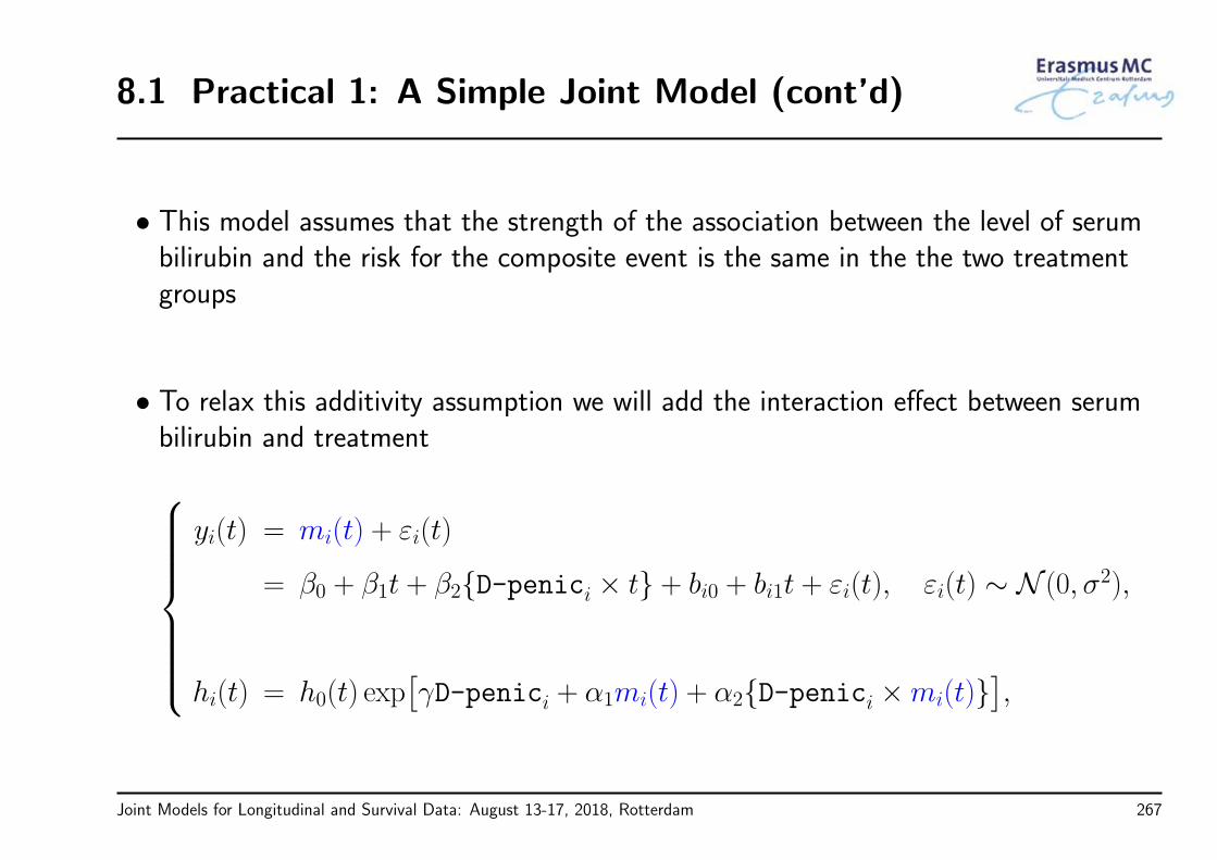
8.1 Practical 1: A Simple Joint Model (cont’d)
• This model assumes that the strength of the association between the level of serumbilirubin and the risk for the composite event is the same in the the two treatmentgroups
• To relax this additivity assumption we will add the interaction effect between serumbilirubin and treatment
yi(t) = mi(t) + εi(t)
= β0 + β1t + β2D-penici × t + bi0 + bi1t + εi(t), εi(t) ∼ N (0, σ2),
hi(t) = h0(t) exp[γD-penici + α1mi(t) + α2D-penici ×mi(t)
],
Joint Models for Longitudinal and Survival Data: August 13-17, 2018, Rotterdam 267

8.1 Practical 1: A Simple Joint Model (cont’d)
• To fit this model with package JM we need to define the interFact argument ofjointModel(). This should be a named list with two elements:
value: a formula with the factors for which we wish to calculate the interactionterms
data: the data frame used to fit the Cox model
• T7: Define this list and fit the corresponding joint model. Use the summary()method to obtained a detailed output and interpret the results
Joint Models for Longitudinal and Survival Data: August 13-17, 2018, Rotterdam 268

8.1 Practical 1: A Simple Joint Model (cont’d)
• Based on the fitted joint model we can test for three treatment effects, namely
in the longitudinal process:
H0 : β2 = 0
in the survival process:
H0 : γ = α2 = 0
in the joint process:
H0 : β2 = γ = α2 = 0
Joint Models for Longitudinal and Survival Data: August 13-17, 2018, Rotterdam 269
8.1 Practical 1: A Simple Joint Model (cont’d)
• We would like test these hypotheses using likelihood ratio tests
• T8: Fit the three joint models under the corresponding H0, and use functionanova() to perform the LRTs (this function accepts as a first argument the joint model under the null,
and as second the joint model under the alternative)
Joint Models for Longitudinal and Survival Data: August 13-17, 2018, Rotterdam 270
8.2 Practical 2: Challenging jointModel()
• T1: Download the workspace DataPract2.RData fromhttp://jmr.r-forge.r-project.org/DataPract2.RData and load it to R (File
→ Load Workspace. . . )
• In this workspace there are the two datasets
dataLong
* patnr: patient id number
* lnY: longitudinal response variable
* obstime: follow-up time
* age: the age of the patients
* gender: the gender of the patients
Joint Models for Longitudinal and Survival Data: August 13-17, 2018, Rotterdam 271

8.2 Practical 2: Challenging jointModel() (cont’d)
and
dataSurv
* eventTime: observed event times
* event: 0 censored, 1 event
* age: the age of the patients
* gender: the gender of the patients
Joint Models for Longitudinal and Survival Data: August 13-17, 2018, Rotterdam 272
8.2 Practical 2: Challenging jointModel() (cont’d)
• We will fit a joint model in which
longitudinal submodel: linear subject-specific random slopes
yi(t) = mi(t) + εi(t)
mi(t) = (β0 + bi0) + (β1 + bi1)t + β2agei + β3genderi
survival submodel: age, gender & the true effect of lnY
hi(t) = h0(t) expγ1agei + γ2genderi + αmi(t)
h0(t) taken piecewise-constant
Joint Models for Longitudinal and Survival Data: August 13-17, 2018, Rotterdam 273

8.2 Practical 2: Challenging jointModel() (cont’d)
• T2: Fit the linear mixed effects model for lnY using function lme(), controlling forage and gender, and assuming a diagonal matrix for the random effects (see pp. 37–41)
• T3: Fit the Cox PH model using coxph() that includes Age and Gender (see pp.
67–68)
• T4: Fit the corresponding joint model based on the fitted linear mixed and Coxmodels using function jointModel() (see pp. 106–108)
with piecewise-constant baseline hazard & the (pseudo) adaptive GH rule
⇒ What do you observe?
Joint Models for Longitudinal and Survival Data: August 13-17, 2018, Rotterdam 274
8.2 Practical 2: Challenging jointModel() (cont’d)
• T5: Refit the joint model setting verbose = TRUE. This will print the parametervalues during the optimization ⇒ What do you observe?
• T6: Refit the joint model by appropriately adjusting the init argument (check the help
page of jointModel() for the syntax)
Joint Models for Longitudinal and Survival Data: August 13-17, 2018, Rotterdam 275
8.3 Practical 3: Using derivForm
• We will fit a joint model for the PBC dataset
longitudinal submodel: linear and quadratic subject-specific random slopes for logserum bilirubin
yi(t) = mi(t) + εi(t)
mi(t) = (β0 + bi0) + (β1 + bi1)t + (β2 + bi2)t2
survival submodel: true effect of log serum bilirubin
hi(t) = h0(t) expαmi(t)
h0(t) taken piecewise-constant
Joint Models for Longitudinal and Survival Data: August 13-17, 2018, Rotterdam 276

8.3 Practical 3: Using derivForm (cont’d)
• Start R and load package JM, using library(JM)
• The longitudinal (long format) and survival information for the PBC patients can befound in data frames pbc2 and pbc2.id. The variables that we will need are:
pbc2
* id: patient id number
* serBilir: serum bilirubin
* year: follow-up times in years
pbc2.id
* years: observed event times in years
* status: ‘alive’, ‘transplanted’, ‘dead’
Joint Models for Longitudinal and Survival Data: August 13-17, 2018, Rotterdam 277
8.3 Practical 3: Using derivForm (cont’d)
• T1: Fit the linear mixed effects model for log serum bilirubin using function lme()
and assuming linear and quadratic evolutions in time for each subject, and a diagonalmatrix for the random effects (see pp. 37–41), i.e.,
yi(t) = mi(t) + εi(t)
mi(t) = (β0 + bi0) + (β1 + bi1)t + (β2 + bi2)t2
• T2: Create the indicator for the composite event (i.e., ‘alive’ = 0, ‘transplanted’ or‘dead’ = 1) using the code
pbc2.id$status2 <- as.numeric(pbc2.id$status != "alive")
Joint Models for Longitudinal and Survival Data: August 13-17, 2018, Rotterdam 278

8.3 Practical 3: Using derivForm (cont’d)
• T3: Fit the null Cox PH model using coxph() that does not include any covariates,remember to set x = TRUE (see pp. 67–68)
• T4: Fit the corresponding joint model based on the fitted linear mixed and Coxmodels using function jointModel() (see pp. 106–108)
with piecewise-constant baseline hazard & the (pseudo) adaptive GH rule
• We want to extend the previous joint model and include the current value and thetime-dependent slope term, i.e.,
hi(t) = h0(t) expα1mi(t) + α2m′i(t)
Joint Models for Longitudinal and Survival Data: August 13-17, 2018, Rotterdam 279

8.3 Practical 3: Using derivForm (cont’d)
• The derivative of mi(t) with respect to time is
m′i(t) =
dmi(t)
dt= (β1 + bi1) + 2(β2 + bi2)t
• To fit this joint model we need to specify the derivForm argument, which is a listwith four elements
fixed: a formula describing the fixed part of m′i(t)
random: a formula describing the random part of m′i(t)
indFixed: index denoting which β of mi(t) are involved in the calculation ofm′i(t)
indRandom: index denoting which bi of mi(t) are involved in the calculation ofm′i(t)
Joint Models for Longitudinal and Survival Data: August 13-17, 2018, Rotterdam 280

8.3 Practical 3: Using derivForm (cont’d)
• Rewriting mi(t) and m′i(t) to split in a fixed and random part
mi(t) = (β0 + β1t + β2t2) + (bi0 + bi1t + bi2t
2)
m′i(t) = (β1 + 2β2t) + (bi1 + 2bi2t)
Thus, the list to supply to derivForm will have the form
dForm <- list(
fixed = ~ I(2*year),
random = ~ I(2*year),
indFixed = c(2,3),
indRandom = c(2,3)
)
Joint Models for Longitudinal and Survival Data: August 13-17, 2018, Rotterdam 281

8.3 Practical 3: Using derivForm (cont’d)
• T5: Fit the joint model that includes both mi(t) and m′i(t) (see pp. 141–142)
you will need to set parameterization = "both", and
for argument derivForm use the dForm list we defined above
Joint Models for Longitudinal and Survival Data: August 13-17, 2018, Rotterdam 282

8.3 Practical 3: Using derivForm (cont’d)
• We would like again to fit the joint model that includes both mi(t) and m′i(t), but
now we would like to model the subject-specific longitudinal profiles more flexiblyusing regression splines
• T6: Re-fit the linear mixed model using natural cubic splines with 3 d.f. To do thisyou need to use function ns() from package splines (which is automatically loadedwhen you load JM)
assume again a diagonal covariance matrix for the random effects
Joint Models for Longitudinal and Survival Data: August 13-17, 2018, Rotterdam 283

8.3 Practical 3: Using derivForm (cont’d)
• To fit the joint models, we again require to appropriately define the derivFormargument
Problem: How can I calculate the derivative of natural cubic spline
Solution: Theoretically a bit difficult, but we can do it easily in practicenumerically (i.e., using numerical derivatives). This is already implemented infunction dns()
T7: Using dns() define the list with the R formulas and index vector for the fixedand random effects, respectively, and fit the joint model
Joint Models for Longitudinal and Survival Data: August 13-17, 2018, Rotterdam 284

8.4 Practical 4: Dynamic Predictions
• We will work with the Liver Cirrhosis dataset
a placebo-controlled randomized trial on 488 liver cirrhosis patients
• Start R and load package JM, using library(JM)
• The longitudinal (long format) and survival information for the liver cirrhosis patientscan be found in data frames prothro and prothros, respectively. The variablesthat we will need are:
Joint Models for Longitudinal and Survival Data: August 13-17, 2018, Rotterdam 285

8.4 Practical 4: Dynamic Predictions (cont’d)
prothro
* id: patient id number
* pro: prothrobin measurements
* time: follow-up times in years
* treat: randomized treatment
prothros
* Time: observed event times in years
* death: event indicator with 0 = ‘alive’, and 1 = ‘dead’
* treat: randomized treatment
Joint Models for Longitudinal and Survival Data: August 13-17, 2018, Rotterdam 286
8.4 Practical 4: Dynamic Predictions (cont’d)
• We will fit the following joint model to the Liver Cirrhosis dataset
longitudinal submodel: linear subject-specific random slopes for prothrobin levelsallowing for different average evolutions in the two treatment groups
yi(t) = mi(t) + εi(t)
mi(t) = β0 + β1t + β2Trti × t + bi0 + bi1t
survival submodel: treatment effect & true effect of prothrobin
hi(t) = h0(t) expγTrti + αmi(t)
h0(t) taken piecewise-constant
Joint Models for Longitudinal and Survival Data: August 13-17, 2018, Rotterdam 287

8.4 Practical 4: Dynamic Predictions (cont’d)
• T1: Fit the linear mixed model using lme(), the Cox model using coxph(), and thecorresponding joint model using jointModel()
• We are interested in producing predictions of survival probabilities for Patient 155
• T2: Extract the data of Patient 155 using the code
dataP155 <- prothro[prothro$id == 155, ]
Joint Models for Longitudinal and Survival Data: August 13-17, 2018, Rotterdam 288

8.4 Practical 4: Dynamic Predictions (cont’d)
• T3: Using the first measurement of Patient 155, and the fitted joint model calculatehis conditional survival probabilities using function survfitJM() and plot it usingthe plot method (see p. 193)
• T4: Repeat the same procedure by including each time the next measurement ofPatient 155 and see how his survival probabilities evolve dynamically in time as extraprothrobin measurements are recorded
check arguments conf.int and fill.area of the plot() method for includingthe 95% confidence intervals
Joint Models for Longitudinal and Survival Data: August 13-17, 2018, Rotterdam 289

8.4 Practical 4: Dynamic Predictions (cont’d)
• T5: Similarly, produce predictions for future longitudinal responses of Patient 155using the predict() method for fitted joint models (see p. 204)
first using only the first measurement,
and following update the predictions after each new longitudinal measurement hasbeen recorded
• T6: Calculate the AUC under the postulated model at year 2 and with a half a yearwindow (see p. 233)
• T7: Do the same for the prediction error (see p. 239)
Joint Models for Longitudinal and Survival Data: August 13-17, 2018, Rotterdam 290