tutorial i: motivation for joint modeling & joint models … · tutorial i: motivation for...
TRANSCRIPT

Tutorial I: Motivation for Joint Modeling & Joint Models forLongitudinal and Survival Data
Dimitris RizopoulosDepartment of Biostatistics, Erasmus University Medical Center
Joint Modeling and BeyondMeeting and Tutorials on Joint Modeling With Survival, Longitudinal, and Missing Data
April 14, 2016, Diepenbeek

Contents
1 Introduction 1
1.1 Motivating Longitudinal Studies . . . . . . . . . . . . . . . . . . . . . . . . . . 2
1.2 Research Questions . . . . . . . . . . . . . . . . . . . . . . . . . . . . . . . 10
1.3 Recent Developments . . . . . . . . . . . . . . . . . . . . . . . . . . . . . . 13
1.4 Joint Models . . . . . . . . . . . . . . . . . . . . . . . . . . . . . . . . . . 15
2 Linear Mixed-Effects Models 18
2.1 Features of Longitudinal Data . . . . . . . . . . . . . . . . . . . . . . . . . . . 19
2.2 The Linear Mixed Model . . . . . . . . . . . . . . . . . . . . . . . . . . . . . 20
Tutorial I: Joint Models for Longitudinal and Survival Data: April 14, 2016 ii
2.3 Missing Data in Longitudinal Studies . . . . . . . . . . . . . . . . . . . . . . . . 29
2.4 Missing Data Mechanisms . . . . . . . . . . . . . . . . . . . . . . . . . . . . 32
3 Relative Risk Models 37
3.1 Features of Survival Data . . . . . . . . . . . . . . . . . . . . . . . . . . . . . 38
3.2 Relative Risk Models . . . . . . . . . . . . . . . . . . . . . . . . . . . . . . . 41
3.3 Time Dependent Covariates . . . . . . . . . . . . . . . . . . . . . . . . . . . . 44
3.4 Extended Cox Model . . . . . . . . . . . . . . . . . . . . . . . . . . . . . . . 49
4 The Basic Joint Model 54
4.1 Joint Modeling Framework . . . . . . . . . . . . . . . . . . . . . . . . . . . . 55
Tutorial I: Joint Models for Longitudinal and Survival Data: April 14, 2016 iii

4.2 Estimation . . . . . . . . . . . . . . . . . . . . . . . . . . . . . . . . . . . 66
4.3 A Comparison with the TD Cox . . . . . . . . . . . . . . . . . . . . . . . . . . 69
4.4 Joint Models in R . . . . . . . . . . . . . . . . . . . . . . . . . . . . . . . . 72
4.5 Connection with Missing Data . . . . . . . . . . . . . . . . . . . . . . . . . . . 78
Tutorial I: Joint Models for Longitudinal and Survival Data: April 14, 2016 iv
What are these Tutorials About
• Often in follow-up studies different types of outcomes are collected
• Explicit outcomes
◃ multiple longitudinal responses (e.g., markers, blood values)
◃ time-to-event(s) of particular interest (e.g., death, relapse)
• Implicit outcomes
◃ missing data (e.g., dropout, intermittent missingness)
◃ random visit times
Tutorial I: Joint Models for Longitudinal and Survival Data: April 14, 2016 v

What are these Tutorials About (cont’d)
• Methods for the separate analysis of such outcomes are well established in theliterature
• Survival data:
◃ Cox model, accelerated failure time models, . . .
• Longitudinal data
◃ mixed effects models, GEE, marginal models, . . .
Tutorial I: Joint Models for Longitudinal and Survival Data: April 14, 2016 vi

What are these Tutorials About (cont’d)
Purpose of these tutorials is to introduce the basics of popular
Joint Modelings Techniques
Tutorial I: Joint Models for Longitudinal and Survival Data: April 14, 2016 vii

Chapter 1
Introduction
Tutorial I: Joint Models for Longitudinal and Survival Data: April 14, 2016 1

1.1 Motivating Longitudinal Studies
• AIDS: 467 HIV infected patients who had failed or were intolerant to zidovudinetherapy (AZT) (Abrams et al., NEJM, 1994)
• The aim of this study was to compare the efficacy and safety of two alternativeantiretroviral drugs, didanosine (ddI) and zalcitabine (ddC)
• Outcomes of interest:
◃ time to death
◃ randomized treatment: 230 patients ddI and 237 ddC
◃ CD4 cell count measurements at baseline, 2, 6, 12 and 18 months
◃ prevOI: previous opportunistic infections
Tutorial I: Joint Models for Longitudinal and Survival Data: April 14, 2016 2

1.1 Motivating Longitudinal Studies (cont’d)
Time (months)
CD
4 ce
ll co
unt
0
5
10
15
20
25
0 5 10 15
ddC
0 5 10 15
ddI
Tutorial I: Joint Models for Longitudinal and Survival Data: April 14, 2016 3

1.1 Motivating Longitudinal Studies (cont’d)
0 5 10 15 20
0.0
0.2
0.4
0.6
0.8
1.0
Kaplan−Meier Estimate
Time (months)
Sur
viva
l Pro
babi
lity
ddC
ddI
Tutorial I: Joint Models for Longitudinal and Survival Data: April 14, 2016 4

1.1 Motivating Longitudinal Studies (cont’d)
• Research Questions:
◃ How strong is the association between CD4 cell count and the risk for death?
◃ Is CD4 cell count a good biomarker?
* if treatment improves CD4 cell count, does it also improve survival?
Tutorial I: Joint Models for Longitudinal and Survival Data: April 14, 2016 5

1.1 Motivating Longitudinal Studies (cont’d)
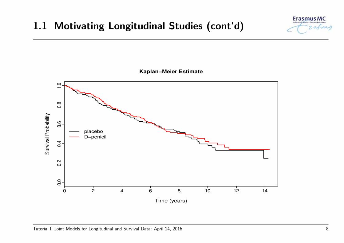
• PBC: Primary Biliary Cirrhosis:
◃ a chronic, fatal but rare liver disease
◃ characterized by inflammatory destruction of the small bile ducts within the liver
• Data collected by Mayo Clinic from 1974 to 1984 (Murtaugh et al., Hepatology, 1994)
• Outcomes of interest:
◃ time to death and/or time to liver transplantation
◃ randomized treatment: 158 patients received D-penicillamine and 154 placebo
◃ longitudinal serum bilirubin levels
Tutorial I: Joint Models for Longitudinal and Survival Data: April 14, 2016 6

1.1 Motivating Longitudinal Studies (cont’d)
Time (years)
log
seru
m B
iliru
bin
−10123
38
0 5 10
39 51
0 5 10
68
70 82 90
−10123
93
−10123
134 148 173 200
0 5 10
216 242
0 5 10
269
−10123
290
Tutorial I: Joint Models for Longitudinal and Survival Data: April 14, 2016 7
1.1 Motivating Longitudinal Studies (cont’d)
0 2 4 6 8 10 12 14
0.0
0.2
0.4
0.6
0.8
1.0
Kaplan−Meier Estimate
Time (years)
Sur
viva
l Pro
babi
lity
placebo
D−penicil
Tutorial I: Joint Models for Longitudinal and Survival Data: April 14, 2016 8
1.1 Motivating Longitudinal Studies (cont’d)
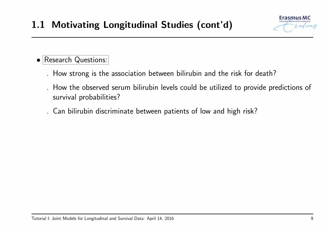
• Research Questions:
◃ How strong is the association between bilirubin and the risk for death?
◃ How the observed serum bilirubin levels could be utilized to provide predictions ofsurvival probabilities?
◃ Can bilirubin discriminate between patients of low and high risk?
Tutorial I: Joint Models for Longitudinal and Survival Data: April 14, 2016 9

1.2 Research Questions
• Depending on the questions of interest, different types of statistical analysis arerequired
• We will distinguish between two general types of analysis
◃ separate analysis per outcome
◃ joint analysis of outcomes
• Focus on each outcome separately
◃ does treatment affect survival?
◃ are the average longitudinal evolutions different between males and females?
◃ . . .
Tutorial I: Joint Models for Longitudinal and Survival Data: April 14, 2016 10

1.2 Research Questions (cont’d)
• Focus on multiple outcomes
◃ Complex hypothesis testing: does treatment improve the average longitudinalprofiles in all markers?
◃ Complex effect estimation: how strong is the association between the longitudinalevolution of CD4 cell counts and the hazard rate for death?
◃ Association structure among outcomes:
* how the association between markers evolves over time (evolution of theassociation)
* how marker-specific evolutions are related to each other (association of theevolutions)
Tutorial I: Joint Models for Longitudinal and Survival Data: April 14, 2016 11

1.2 Research Questions (cont’d)
◃ Prediction: can we improve prediction for the time to death by considering allmarkers simultaneously?
◃ Handling implicit outcomes: focus on a single longitudinal outcome but withdropout or random visit times
Tutorial I: Joint Models for Longitudinal and Survival Data: April 14, 2016 12

1.3 Recent Developments
• Up to now emphasis has been
◃ restricted or coerced to separate analysis per outcome
◃ or given to naive types of joint analysis (e.g., last observation carried forward)
• Main reasons
◃ lack of appropriate statistical methodology
◃ lack of efficient computational approaches & software
Tutorial I: Joint Models for Longitudinal and Survival Data: April 14, 2016 13

1.3 Recent Developments (cont’d)
• However, recently there has been an explosion in the statistics and biostatisticsliterature of joint modeling approaches
• Many different approaches have been proposed that
◃ can handle different types of outcomes
◃ can be utilized in pragmatic computing time
◃ can be rather flexible
◃ most importantly: can answer the questions of interest
Tutorial I: Joint Models for Longitudinal and Survival Data: April 14, 2016 14

1.4 Joint Models
• Let Y1 and Y2 two outcomes of interest measured on a number of subjects for whichjoint modeling is of scientific interest
◃ both can be measured longitudinally
◃ one longitudinal and one survival
• We have various possible approaches to construct a joint density p(y1, y2) of {Y1, Y2}◃ Conditional models: p(y1, y2) = p(y1)p(y2 | y1)
◃ Copulas: p(y1, y2) = c{F(y1),F(y2)}p(y1)p(y2)
But Random Effects Models have (more or less) prevailed
Tutorial I: Joint Models for Longitudinal and Survival Data: April 14, 2016 15

1.4 Joint Models (cont’d)
• Random Effects Models specify
p(y1, y2) =
∫p(y1, y2 | b) p(b) db
=
∫p(y1 | b) p(y2 | b) p(b) db
◃ Unobserved random effects b explain the association between Y1 and Y2
◃ Conditional Independence assumption
Y1 ⊥⊥ Y2 | b
Tutorial I: Joint Models for Longitudinal and Survival Data: April 14, 2016 16

1.4 Joint Models (cont’d)
• Features:
◃ Y1 and Y2 can be of different type
* one continuous and one categorical
* one continuous and one survival
* . . .
◃ Extensions to more than two outcomes straightforward
◃ Specific association structure between Y1 and Y2 is assumed
◃ Computationally intensive (especially in high dimensions)
Tutorial I: Joint Models for Longitudinal and Survival Data: April 14, 2016 17

Chapter 2
Linear Mixed-Effects Models
Tutorial I: Joint Models for Longitudinal and Survival Data: April 14, 2016 18

2.1 Features of Longitudinal Data
• Repeated evaluations of the same outcome in each subject in time
◃ CD4 cell count in HIV-infected patients
◃ serum bilirubin in PBC patients
Measurements on the same subject are expected tobe (positively) correlated
• This implies that standard statistical tools, such as the t-test and simple linearregression that assume independent observations, are not optimal for longitudinaldata analysis.
Tutorial I: Joint Models for Longitudinal and Survival Data: April 14, 2016 19
2.2 The Linear Mixed Model
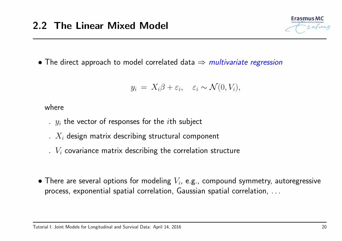
• The direct approach to model correlated data ⇒ multivariate regression
yi = Xiβ + εi, εi ∼ N (0, Vi),
where
◃ yi the vector of responses for the ith subject
◃ Xi design matrix describing structural component
◃ Vi covariance matrix describing the correlation structure
• There are several options for modeling Vi, e.g., compound symmetry, autoregressiveprocess, exponential spatial correlation, Gaussian spatial correlation, . . .
Tutorial I: Joint Models for Longitudinal and Survival Data: April 14, 2016 20

2.2 The Linear Mixed Model (cont’d)
• Alternative intuitive approach: Each subject in the population has her ownsubject-specific mean response profile over time
Tutorial I: Joint Models for Longitudinal and Survival Data: April 14, 2016 21

2.2 The Linear Mixed Model (cont’d)
0 1 2 3 4 5
020
4060
80
Time
Long
itudi
nal O
utco
me
Subject 1
Subject 2
Tutorial I: Joint Models for Longitudinal and Survival Data: April 14, 2016 22
2.2 The Linear Mixed Model (cont’d)
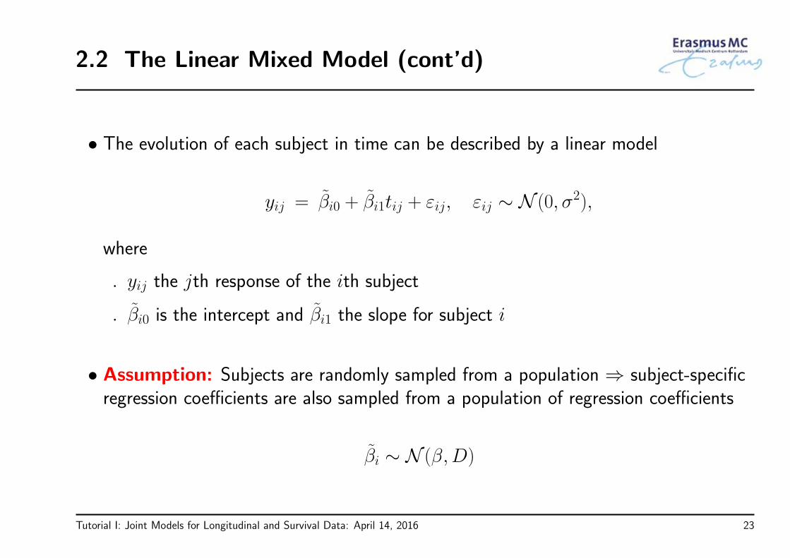
• The evolution of each subject in time can be described by a linear model
yij = β̃i0 + β̃i1tij + εij, εij ∼ N (0, σ2),
where
◃ yij the jth response of the ith subject
◃ β̃i0 is the intercept and β̃i1 the slope for subject i
• Assumption: Subjects are randomly sampled from a population ⇒ subject-specificregression coefficients are also sampled from a population of regression coefficients
β̃i ∼ N (β,D)
Tutorial I: Joint Models for Longitudinal and Survival Data: April 14, 2016 23

2.2 The Linear Mixed Model (cont’d)
• We can reformulate the model as
yij = (β0 + bi0) + (β1 + bi1)tij + εij,
where
◃ βs are known as the fixed effects
◃ bis are known as the random effects
• In accordance for the random effects we assume
bi =
bi0bi1
∼ N (0, D)
Tutorial I: Joint Models for Longitudinal and Survival Data: April 14, 2016 24

2.2 The Linear Mixed Model (cont’d)
• Put in a general formyi = Xiβ + Zibi + εi,
bi ∼ N (0, D), εi ∼ N (0, σ2Ini),
with
◃ X design matrix for the fixed effects β
◃ Z design matrix for the random effects bi
◃ bi ⊥⊥ εi
Tutorial I: Joint Models for Longitudinal and Survival Data: April 14, 2016 25
2.2 The Linear Mixed Model (cont’d)
• Interpretation:
◃ βj denotes the change in the average yi when xj is increased by one unit
◃ bi are interpreted in terms of how a subset of the regression parameters for the ithsubject deviates from those in the population
• Advantageous feature: population + subject-specific predictions
◃ β describes mean response changes in the population
◃ β + bi describes individual response trajectories
Tutorial I: Joint Models for Longitudinal and Survival Data: April 14, 2016 26

2.2 The Linear Mixed Model (cont’d)
• Example: We fit a linear mixed model for the AIDS dataset assuming
◃ different average longitudinal evolutions per treatment group (fixed part)
◃ random intercepts & random slopes (random part)
yij = β0 + β1tij + β2{ddIi × tij} + bi0 + bi1tij + εij,
bi ∼ N (0, D), εij ∼ N (0, σ2)
• Note: We did not include a main effect for treatment due to randomization
Tutorial I: Joint Models for Longitudinal and Survival Data: April 14, 2016 27

2.2 The Linear Mixed Model (cont’d)
Value Std.Err. t-value p-value
β0 7.189 0.222 32.359 < 0.001
β1 −0.163 0.021 −7.855 < 0.001
β2 0.028 0.030 0.952 0.342
• No evidence of differences in the average longitudinal evolutions between the twotreatments
Tutorial I: Joint Models for Longitudinal and Survival Data: April 14, 2016 28

2.3 Missing Data in Longitudinal Studies
• A major challenge for the analysis of longitudinal data is the problem of missing data
◃ studies are designed to collect data on every subject at a set of prespecifiedfollow-up times
◃ often subjects miss some of their planned measurements for a variety of reasons
Tutorial I: Joint Models for Longitudinal and Survival Data: April 14, 2016 29

2.3 Missing Data in Longitudinal Studies (cont’d)
• Implications of missingness:
◃ we collect less data than originally planned ⇒ loss of efficiency
◃ not all subjects have the same number of measurements ⇒ unbalanced datasets
◃ missingness may depend on outcome ⇒ potential bias
• For the handling of missing data, we introduce the missing data indicator
rij =
1 if yij is observed
0 otherwise
Tutorial I: Joint Models for Longitudinal and Survival Data: April 14, 2016 30

2.3 Missing Data in Longitudinal Studies (cont’d)
• We obtain a partition of the complete response vector yi
◃ observed data yoi , containing those yij for which rij = 1
◃ missing data ymi , containing those yij for which rij = 0
• For the remaining we will focus on dropout ⇒ notation can be simplified
◃ Discrete dropout time: rdi = 1 +ni∑j=1
rij (ordinal variable)
◃ Continuous time: T ∗i denotes the time to dropout
Tutorial I: Joint Models for Longitudinal and Survival Data: April 14, 2016 31

2.4 Missing Data Mechanisms
• To describe the probabilistic relation between the measurement and missingnessprocesses Rubin (1976, Biometrika) has introduced three mechanisms
• Missing Completely At Random (MCAR): The probability that responses are missingis unrelated to both yoi and ymi
p(ri | yoi , ymi ) = p(ri)
• Examples
◃ subjects go out of the study after providing a pre-determined number ofmeasurements
◃ laboratory measurements are lost due to equipment malfunction
Tutorial I: Joint Models for Longitudinal and Survival Data: April 14, 2016 32
2.4 Missing Data Mechanisms (cont’d)
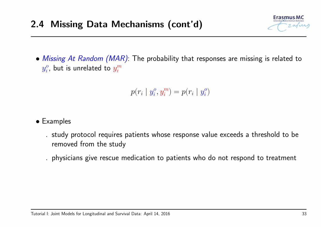
• Missing At Random (MAR): The probability that responses are missing is related toyoi , but is unrelated to ymi
p(ri | yoi , ymi ) = p(ri | yoi )
• Examples
◃ study protocol requires patients whose response value exceeds a threshold to beremoved from the study
◃ physicians give rescue medication to patients who do not respond to treatment
Tutorial I: Joint Models for Longitudinal and Survival Data: April 14, 2016 33
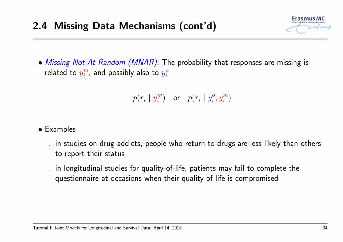
2.4 Missing Data Mechanisms (cont’d)
• Missing Not At Random (MNAR): The probability that responses are missing isrelated to ymi , and possibly also to yoi
p(ri | ymi ) or p(ri | yoi , ymi )
• Examples
◃ in studies on drug addicts, people who return to drugs are less likely than othersto report their status
◃ in longitudinal studies for quality-of-life, patients may fail to complete thequestionnaire at occasions when their quality-of-life is compromised
Tutorial I: Joint Models for Longitudinal and Survival Data: April 14, 2016 34
2.4 Missing Data Mechanisms (cont’d)
• Features of MNAR
◃ The observed data cannot be considered a random sample from the targetpopulation
◃ Only procedures that explicitly model the joint distribution {yoi , ymi , ri} providevalid inferences ⇒ analyses which are valid under MAR will not be validunder MNAR
Tutorial I: Joint Models for Longitudinal and Survival Data: April 14, 2016 35
2.4 Missing Data Mechanisms (cont’d)
We cannot tell from the data at hand whether themissing data mechanism is MAR or MNAR
Note: We can distinguish between MCAR and MAR
Tutorial I: Joint Models for Longitudinal and Survival Data: April 14, 2016 36

Chapter 3
Relative Risk Models
Tutorial I: Joint Models for Longitudinal and Survival Data: April 14, 2016 37

3.1 Features of Survival Data
• The most important characteristic that distinguishes the analysis of time-to-eventoutcomes from other areas in statistics is Censoring
◃ the event time of interest is not fully observed for all subjects under study
• Implications of censoring:
◃ standard tools, such as the sample average, the t-test, and linear regressioncannot be used
◃ inferences may be sensitive to misspecification of the distribution of the eventtimes
Tutorial I: Joint Models for Longitudinal and Survival Data: April 14, 2016 38

3.1 Features of Survival Data (cont’d)
• Several types of censoring:
◃ Location of the true event time wrt the censoring time: right, left & interval
◃ Probabilistic relation between the true event time & the censoring time:informative & non-informative (similar to MNAR and MAR)
Here we focus on non-informative right censoring
• Note: Survival times may often be truncated; analysis of truncated samples requiressimilar calculations as censoring
Tutorial I: Joint Models for Longitudinal and Survival Data: April 14, 2016 39

3.1 Features of Survival Data (cont’d)
• Notation (i denotes the subject)
◃ T ∗i ‘true’ time-to-event
◃ Ci the censoring time (e.g., the end of the study or a random censoring time)
• Available data for each subject
◃ observed event time: Ti = min(T ∗i , Ci)
◃ event indicator: δi = 1 if event; δi = 0 if censored
Our aim is to make valid inferences for T ∗i but using
only {Ti, δi}
Tutorial I: Joint Models for Longitudinal and Survival Data: April 14, 2016 40

3.2 Relative Risk Models
• Relative Risk Models assume a multiplicative effect of covariates on the hazardscale, i.e.,
hi(t) = h0(t) exp(γ1wi1 + γ2wi2 + . . . + γpwip) ⇒
log hi(t) = log h0(t) + γ1wi1 + γ2wi2 + . . . + γpwip,
where
◃ hi(t) denotes the hazard for an event for patient i at time t
◃ h0(t) denotes the baseline hazard
◃ wi1, . . . , wip a set of covariates
Tutorial I: Joint Models for Longitudinal and Survival Data: April 14, 2016 41

3.2 Relative Risk Models (cont’d)
• Cox Model: We make no assumptions for the baseline hazard function
• Parameter estimates and standard errors are based on the log partial likelihoodfunction
pℓ(γ) =
n∑i=1
δi
[γ⊤wi − log
{ ∑j:Tj≥Ti
exp(γ⊤wj)}]
,
where only patients who had an event contribute
Tutorial I: Joint Models for Longitudinal and Survival Data: April 14, 2016 42

3.2 Relative Risk Models (cont’d)
• Example: For the PBC dataset were interested in the treatment effect whilecorrecting for sex and age effects
hi(t) = h0(t) exp(γ1D-penici + γ2Femalei + γ3Agei)
Value HR Std.Err. z-value p-value
γ1 −0.138 0.871 0.156 −0.882 0.378
γ2 −0.493 0.611 0.207 −2.379 0.017
γ3 0.021 1.022 0.008 2.784 0.005
Tutorial I: Joint Models for Longitudinal and Survival Data: April 14, 2016 43

3.3 Time Dependent Covariates
• Often interest in the association between a time-dependent covariate and the risk foran event
◃ treatment changes with time (e.g., dose)
◃ time-dependent exposure (e.g., smoking, diet)
◃ markers of disease or patient condition (e.g., blood pressure, PSA levels)
◃ . . .
• Example: In the PBC study, are the longitudinal bilirubin measurements associatedwith the hazard for death?
Tutorial I: Joint Models for Longitudinal and Survival Data: April 14, 2016 44

3.3 Time Dependent Covariates (cont’d)
• To answer our questions of interest we need to postulate a model that relates
◃ the serum bilirubin with
◃ the time-to-death
• The association between baseline marker levels and the risk for death can beestimated with standard statistical tools (e.g., Cox regression)
• When we move to the time-dependent setting, a more careful consideration isrequired
Tutorial I: Joint Models for Longitudinal and Survival Data: April 14, 2016 45

3.3 Time Dependent Covariates (cont’d)
• There are two types of time-dependent covariates(Kalbfleisch and Prentice, 2002, Section 6.3)
◃ Exogenous (aka external): the future path of the covariate up to any time t > s isnot affected by the occurrence of an event at time point s, i.e.,
Pr{Yi(t) | Yi(s), T
∗i ≥ s
}= Pr
{Yi(t) | Yi(s), T
∗i = s
},
where 0 < s ≤ t and Yi(t) = {yi(s), 0 ≤ s < t}
◃ Endogenous (aka internal): not Exogenous
Tutorial I: Joint Models for Longitudinal and Survival Data: April 14, 2016 46

3.3 Time Dependent Covariates (cont’d)
• It is very important to distinguish between these two types of time-dependentcovariates, because the type of covariate dictates the appropriate type of analysis
• In our motivating examples all time-varying covariates are Biomarkers ⇒ These arealways endogenous covariates
◃ measured with error (i.e., biological variation)
◃ the complete history is not available
◃ existence directly related to failure status
Tutorial I: Joint Models for Longitudinal and Survival Data: April 14, 2016 47
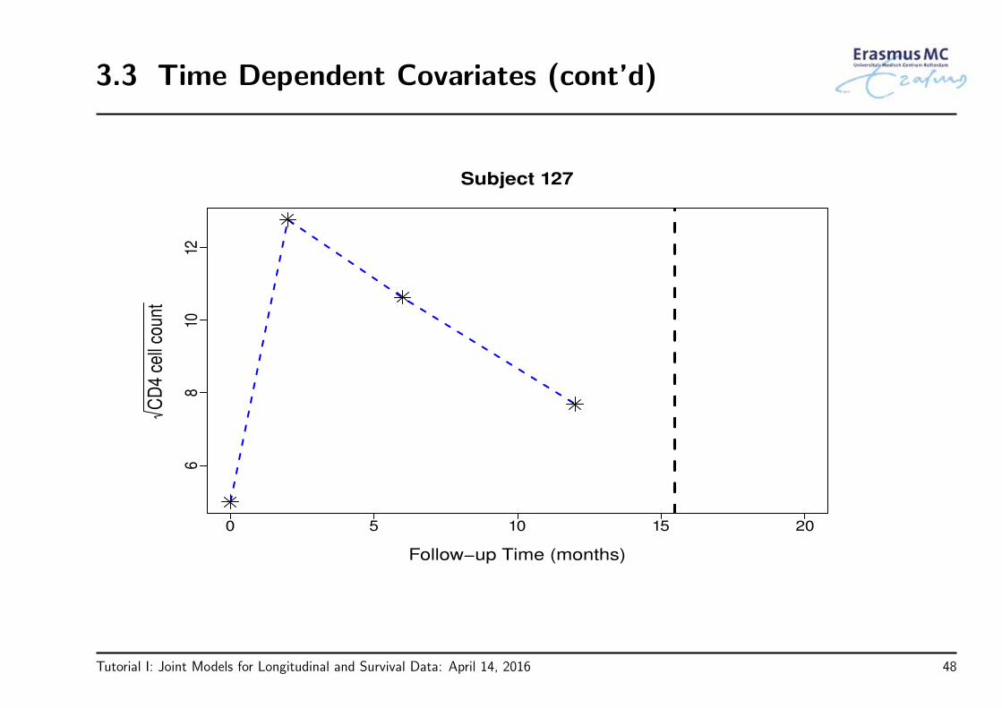
3.3 Time Dependent Covariates (cont’d)
0 5 10 15 20
68
1012Subject 127
Follow−up Time (months)
CD
4 ce
ll co
unt
Tutorial I: Joint Models for Longitudinal and Survival Data: April 14, 2016 48

3.4 Extended Cox Model
• The Cox model presented earlier can be extended to handle time-dependentcovariates using the counting process formulation
hi(t | Yi(t), wi) = h0(t)Ri(t) exp{γ⊤wi + αyi(t)},
where
◃ Ni(t) is a counting process which counts the number of events for subject i bytime t,
◃ hi(t) denotes the intensity process for Ni(t),
◃ Ri(t) denotes the at risk process (‘1’ if subject i still at risk at t), and
◃ yi(t) denotes the value of the time-varying covariate at t
Tutorial I: Joint Models for Longitudinal and Survival Data: April 14, 2016 49

3.4 Extended Cox Model (cont’d)
• Interpretation:
hi(t | Yi(t), wi) = h0(t)Ri(t) exp{γ⊤wi + αyi(t)}
exp(α) denotes the relative increase in the risk for an event at time t that resultsfrom one unit increase in yi(t) at the same time point
• Parameters are estimated based on the log-partial likelihood function
pℓ(γ, α) =
n∑i=1
∫ ∞
0
{Ri(t) exp{γ⊤wi + αyi(t)}
− log[∑
j
Rj(t) exp{γ⊤wj + αyj(t)}]}
dNi(t)
Tutorial I: Joint Models for Longitudinal and Survival Data: April 14, 2016 50

3.4 Extended Cox Model (cont’d)
• How does the extended Cox model handle time-varying covariates?
◃ assumes no measurement error
◃ step-function path
◃ existence of the covariate is not related to failure status
Tutorial I: Joint Models for Longitudinal and Survival Data: April 14, 2016 51

3.4 Extended Cox Model (cont’d)
Time
0.1
0.2
0.3
0.4
hazard function
−0.
50.
00.
51.
01.
52.
0
0 2 4 6 8 10
longitudinal outcome
Tutorial I: Joint Models for Longitudinal and Survival Data: April 14, 2016 52

3.4 Extended Cox Model (cont’d)
• Therefore, the extended Cox model is only valid for exogenous time-dependentcovariates
Treating endogenous covariates as exogenous mayproduce spurious results!
Tutorial I: Joint Models for Longitudinal and Survival Data: April 14, 2016 53

Chapter 4
The Basic Joint Model
Tutorial I: Joint Models for Longitudinal and Survival Data: April 14, 2016 54

4.1 Joint Modeling Framework
• To account for the special features of endogenous covariates a new class of modelshas been developed
Joint Models for Longitudinal and Time-to-Event Data
• Intuitive idea behind these models
1. use an appropriate model to describe the evolution of the marker in time for eachpatient
2. the estimated evolutions are then used in a Cox model
• Feature: Marker level’s are not assumed constant between visits
Tutorial I: Joint Models for Longitudinal and Survival Data: April 14, 2016 55

4.1 Joint Modeling Framework (cont’d)
Time
0.1
0.2
0.3
0.4
hazard function
−0.
50.
00.
51.
01.
52.
0
0 2 4 6 8 10
longitudinal outcome
Tutorial I: Joint Models for Longitudinal and Survival Data: April 14, 2016 56

4.1 Joint Modeling Framework (cont’d)
• Some notation
◃ T ∗i : True event time for patient i
◃ Ti: Observed event time for patient i
◃ δi: Event indicator, i.e., equals 1 for true events
◃ yi: Longitudinal responses
• We will formulate the joint model in 3 steps – in particular, . . .
Tutorial I: Joint Models for Longitudinal and Survival Data: April 14, 2016 57

4.1 Joint Modeling Framework (cont’d)
• Step 1: Let’s assume that we know mi(t), i.e., the true & unobserved value of themarker at time t
• Then, we can define a standard relative risk model
hi(t | Mi(t)) = h0(t) exp{γ⊤wi + αmi(t)},
where
◃ Mi(t) = {mi(s), 0 ≤ s < t} longitudinal history
◃ α quantifies the strength of the association between the marker and the risk foran event
◃ wi baseline covariates
Tutorial I: Joint Models for Longitudinal and Survival Data: April 14, 2016 58

4.1 Joint Modeling Framework (cont’d)
• Step 2: From the observed longitudinal response yi(t) reconstruct the covariatehistory for each subject
• Mixed effects model (we focus, for now, on continuous markers)
yi(t) = mi(t) + εi(t)
= x⊤i (t)β + z⊤i (t)bi + εi(t), εi(t) ∼ N (0, σ2),
where
◃ xi(t) and β: Fixed-effects part
◃ zi(t) and bi: Random-effects part, bi ∼ N (0, D)
Tutorial I: Joint Models for Longitudinal and Survival Data: April 14, 2016 59

4.1 Joint Modeling Framework (cont’d)
• Step 3: The two processes are associated ⇒ define a model for their jointdistribution
• Joint Models for such joint distributions are of the following form(Tsiatis & Davidian, Stat. Sinica, 2004)
p(yi, Ti, δi) =
∫p(yi | bi)
{h(Ti | bi)δi S(Ti | bi)
}p(bi) dbi,
where
◃ bi a vector of random effects that explains the interdependencies
◃ p(·) density function; S(·) survival function
Tutorial I: Joint Models for Longitudinal and Survival Data: April 14, 2016 60

4.1 Joint Modeling Framework (cont’d)
• Key assumption: Full Conditional Independence ⇒ random effects explain allinterdependencies
◃ the longitudinal outcome is independent of the time-to-event outcome
◃ the repeated measurements in the longitudinal outcome are independent of eachother
p(yi, Ti, δi | bi) = p(yi | bi) p(Ti, δi | bi)
p(yi | bi) =∏j
p(yij | bi)
Caveat: CI is difficult to be tested
Tutorial I: Joint Models for Longitudinal and Survival Data: April 14, 2016 61

4.1 Joint Modeling Framework (cont’d)
• The censoring and visiting∗ processes are assumed non-informative:
• Decision to withdraw from the study or appear for the next visit
◃ may depend on observed past history (baseline covariates + observedlongitudinal responses)
◃ no additional dependence on underlying, latent subject characteristicsassociated with prognosis
∗The visiting process is defined as the mechanism (stochastic or deterministic) that generates the time points at which
longitudinal measurements are collected.
Tutorial I: Joint Models for Longitudinal and Survival Data: April 14, 2016 62

4.1 Joint Modeling Framework (cont’d)
• The survival function, which is a part of the likelihood of the model, depends on thewhole longitudinal history
Si(t | bi) = exp
(−∫ t
0
h0(s) exp{γ⊤wi + αmi(s)} ds
)
• Therefore, care in the definition of the design matrices of the mixed model
◃ when subjects have nonlinear profiles ⇒
◃ use splines or polynomials to model them flexibly
Tutorial I: Joint Models for Longitudinal and Survival Data: April 14, 2016 63

4.1 Joint Modeling Framework (cont’d)
• Assumptions for the baseline hazard function h0(t)
◃ parametric ⇒ possibly restrictive
◃ unspecified ⇒ within JM framework underestimates standard errors
• It is advisable to use parametric but flexible models for h0(t)
◃ splines
log h0(t) = γh0,0 +
Q∑q=1
γh0,qBq(t, v),
where
* Bq(t, v) denotes the q-th basis function of a B-spline with knots v1, . . . , vQ
* γh0 a vector of spline coefficients
Tutorial I: Joint Models for Longitudinal and Survival Data: April 14, 2016 64

4.1 Joint Modeling Framework (cont’d)
• It is advisable to use parametric but flexible models for h0(t)
◃ step-functions: piecewise-constant baseline hazard often works satisfactorily
h0(t) =
Q∑q=1
ξqI(vq−1 < t ≤ vq),
where 0 = v0 < v1 < · · · < vQ denotes a split of the time scale
Tutorial I: Joint Models for Longitudinal and Survival Data: April 14, 2016 65

4.2 Estimation
• Mainly maximum likelihood but also Bayesian approaches
• The log-likelihood contribution for subject i:
ℓi(θ) = log
∫ { ni∏j=1
p(yij | bi; θ)}{
h(Ti | bi; θ)δi Si(Ti | bi; θ)}p(bi; θ) dbi,
where
Si(t | bi; θ) = exp
(−∫ t
0
h0(s; θ) exp{γ⊤wi + αmi(s)} ds
)
Tutorial I: Joint Models for Longitudinal and Survival Data: April 14, 2016 66

4.2 Estimation (cont’d)
• Both integrals do not have, in general, a closed-form solution ⇒ need to beapproximated numerically
• Standard numerical integration algorithms
◃ Gaussian quadrature
◃ Monte Carlo
◃ . . .
• More difficult is the integral with respect to bi because it can be of high dimension
◃ Laplace approximations
◃ pseudo-adaptive Gaussian quadrature rules
Tutorial I: Joint Models for Longitudinal and Survival Data: April 14, 2016 67

4.2 Estimation (cont’d)
• To maximize the approximated log-likelihood
ℓ(θ) =
n∑i=1
log
∫p(yi | bi; θ)
{h(Ti | bi; θ)δi Si(Ti | bi; θ)
}p(bi; θ) dbi,
we need to employ an optimization algorithm
• Standard choices
◃ EM (treating bi as missing data)
◃ Newton-type
◃ hybrids (start with EM and continue with quasi-Newton)
Tutorial I: Joint Models for Longitudinal and Survival Data: April 14, 2016 68

4.3 A Comparison with the TD Cox
• Example: To illustrate the virtues of joint modeling, we compare it with the standardtime-dependent Cox model for the AIDS data
yi(t) = mi(t) + εi(t)
= β0 + β1t + β2{t× ddIi} + bi0 + bi1t + εi(t), εi(t) ∼ N (0, σ2),
hi(t) = h0(t) exp{γddIi + αmi(t)},
where
◃ h0(t) is assumed piecewise-constant
Tutorial I: Joint Models for Longitudinal and Survival Data: April 14, 2016 69

4.3 A Comparison with the TD Cox (cont’d)
JM Cox
log HR (std.err) log HR (std.err)
Treat 0.33 (0.16) 0.31 (0.15)
CD41/2 −0.29 (0.04) −0.19 (0.02)
• Clearly, there is a considerable effect of ignoring the measurement error, especially forthe CD4 cell counts
Tutorial I: Joint Models for Longitudinal and Survival Data: April 14, 2016 70

4.3 A Comparison with the TD Cox (cont’d)
• A unit decrease in CD41/2, results in a
◃ Joint Model: 1.3-fold increase in risk (95% CI: 1.24; 1.43)
◃ Time-Dependent Cox: 1.2-fold increase in risk (95% CI: 1.16; 1.27)
• Which one to believe?
◃ a lot of theoretical and simulation work has shown that the Cox modelunderestimates the true association size of markers
Tutorial I: Joint Models for Longitudinal and Survival Data: April 14, 2016 71

4.4 Joint Models in R
R> Joint models are fitted using function jointModel() from package JM. Thisfunction accepts as main arguments a linear mixed model and a Cox PH model basedon which it fits the corresponding joint model
lmeFit <- lme(CD4 ~ obstime + obstime:drug,
random = ~ obstime | patient, data = aids)
coxFit <- coxph(Surv(Time, death) ~ drug, data = aids.id, x = TRUE)
jointFit <- jointModel(lmeFit, coxFit, timeVar = "obstime",
method = "piecewise-PH-aGH")
summary(jointFit)
Tutorial I: Joint Models for Longitudinal and Survival Data: April 14, 2016 72
4.4 Joint Models in R (cont’d)
R> The data frame given in lme() should be in the long format, while the data framegiven to coxph() should have one line per subject∗
◃ the ordering of the subjects needs to be the same
R> In the call to coxph() you need to set x = TRUE (or model = TRUE) such thatthe design matrix used in the Cox model is returned in the object fit
R> Argument timeVar specifies the time variable in the linear mixed model
∗ Unless you want to include exogenous time-varying covariates or handle competing risks
Tutorial I: Joint Models for Longitudinal and Survival Data: April 14, 2016 73

4.4 Joint Models in R (cont’d)
R> Argument method specifies the type of relative risk model and the type of numericalintegration algorithm – the syntax is as follows:
<baseline hazard>-<parameterization>-<numerical integration>
Available options are:
◃ "piecewise-PH-GH": PH model with piecewise-constant baseline hazard
◃ "spline-PH-GH": PH model with B-spline-approximated log baseline hazard
◃ "weibull-PH-GH": PH model with Weibull baseline hazard
◃ "weibull-AFT-GH": AFT model with Weibull baseline hazard
◃ "Cox-PH-GH": PH model with unspecified baseline hazard
GH stands for standard Gauss-Hermite; using aGH invokes the pseudo-adaptiveGauss-Hermite rule
Tutorial I: Joint Models for Longitudinal and Survival Data: April 14, 2016 74

4.4 Joint Models in R (cont’d)
R> Joint models under the Bayesian approach are fitted using functionjointModelBayes() from package JMbayes. This function works in a very similarmanner as function jointModel(), e.g.,
lmeFit <- lme(CD4 ~ obstime + obstime:drug,
random = ~ obstime | patient, data = aids)
coxFit <- coxph(Surv(Time, death) ~ drug, data = aids.id, x = TRUE)
jointFitBayes <- jointModelBayes(lmeFit, coxFit, timeVar = "obstime")
summary(jointFitBayes)
Tutorial I: Joint Models for Longitudinal and Survival Data: April 14, 2016 75
4.4 Joint Models in R (cont’d)
R> JMbayes is more flexible (in some respects):
◃ directly implements the MCMC
◃ allows for categorical longitudinal data as well
◃ allows for general transformation functions
◃ penalized B-splines for the baseline hazard function
◃ . . .
Tutorial I: Joint Models for Longitudinal and Survival Data: April 14, 2016 76

4.4 Joint Models in R (cont’d)
R> In both packages methods are available for the majority of the standard genericfunctions + extras
◃ summary(), anova(), vcov(), logLik()
◃ coef(), fixef(), ranef()
◃ fitted(), residuals()
◃ plot()
◃ xtable() (you need to load package xtable first)
Tutorial I: Joint Models for Longitudinal and Survival Data: April 14, 2016 77

4.5 Connection with Missing Data
• So far we have attacked the problem from the survival point of view
• However, often, we may be also interested on the longitudinal outcome
• Issue: When patients experience the event, they dropout from the study
◃ a direct connection with the missing data field
Tutorial I: Joint Models for Longitudinal and Survival Data: April 14, 2016 78

4.5 Connection with Missing Data (cont’d)
• To show this connection more clearly
◃ T ∗i : true time-to-event
◃ yoi : longitudinal measurements before T∗i
◃ ymi : longitudinal measurements after T∗i
• Important to realize that the model we postulate for the longitudinal responses isfor the complete vector {yoi , ymi }
◃ implicit assumptions about missingness
Tutorial I: Joint Models for Longitudinal and Survival Data: April 14, 2016 79

4.5 Connection with Missing Data (cont’d)
• Missing data mechanism:
p(T ∗i | yoi , ymi ) =
∫p(T ∗
i | bi) p(bi | yoi , ymi ) dbi
still depends on ymi , which corresponds to nonrandom dropout
Intuitive interpretation: Patients who dropout showdifferent longitudinal evolutions than patients who do not
Tutorial I: Joint Models for Longitudinal and Survival Data: April 14, 2016 80

4.5 Connection with Missing Data (cont’d)
• Joint models belong to the class of Shared Parameter Models
p(yoi , ymi , T
∗i ) =
∫p(yoi , y
mi | bi) p(T ∗
i | bi) p(bi)dbi
the association between the longitudinal and missingness processes is explained bythe shared random effects bi
Tutorial I: Joint Models for Longitudinal and Survival Data: April 14, 2016 81

4.5 Connection with Missing Data (cont’d)
• The other two well-known frameworks for MNAR data are
◃ Selection models
p(yoi , ymi , T
∗i ) = p(yoi , y
mi ) p(T
∗i | yoi , ymi )
◃ Pattern mixture models:
p(yoi , ymi , T
∗i ) = p(yoi , y
mi | T ∗
i ) p(T∗i )
• These two model families are primarily applied with discrete dropout times andcannot be easily extended to continuous time
Tutorial I: Joint Models for Longitudinal and Survival Data: April 14, 2016 82

4.5 Connection with Missing Data (cont’d)
• Example: In the AIDS data the association parameter α was highly significant,suggesting nonrandom dropout
• A comparison between
◃ linear mixed-effects model ⇒ MAR
◃ joint model ⇒ MNAR
is warranted
• MAR assumes that missingness depends only on the observed data
p(T ∗i | yoi , ymi ) = p(T ∗
i | yoi )
Tutorial I: Joint Models for Longitudinal and Survival Data: April 14, 2016 83
4.5 Connection with Missing Data (cont’d)
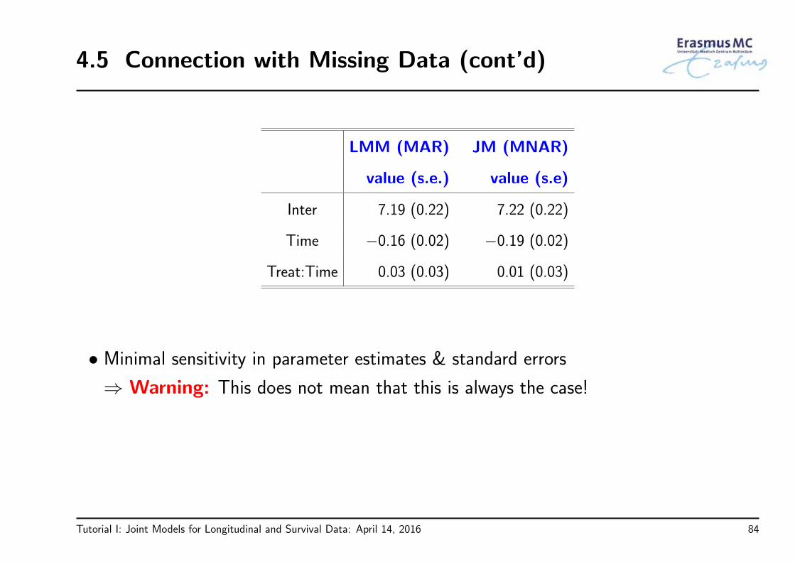
LMM (MAR) JM (MNAR)
value (s.e.) value (s.e)
Inter 7.19 (0.22) 7.22 (0.22)
Time −0.16 (0.02) −0.19 (0.02)
Treat:Time 0.03 (0.03) 0.01 (0.03)
• Minimal sensitivity in parameter estimates & standard errors
⇒ Warning: This does not mean that this is always the case!
Tutorial I: Joint Models for Longitudinal and Survival Data: April 14, 2016 84

The End of Tutorial I!
Tutorial I: Joint Models for Longitudinal and Survival Data: April 14, 2016 85