What Moves the Stock and Bond Markets? A Variance

Decomposition for Long-Term Asset Returns

The Harvard community has made this article openlyavailable.

Please share how this access benefits you. Your storymatters.

Citation Campbell, John Y., and John Ammer. 1993. What movesthe stock and bond markets? A variance decomposition forlong-term asset returns. Journal of Finance 48(1): 3-37.

Published

Version

doi:10.2307/2328880

Accessed August 6, 2014 5:18:05 PM EDT

Citable Link http://nrs.harvard.edu/urn-3:HUL.InstRepos:3382857

Terms of Use This article was downloaded from Harvard University'sDASH repository, and is made available under the termsand conditions applicable to Other Posted Material, as setforth at http://nrs.harvard.edu/urn-3:HUL.InstRepos:dash.current.terms-of-use#LAA

NBER WORKING PAPER SERIES

WHAT MOVES THE STOCK AND BOND MARKETS?A VARIANCE DECOMPOSITION FOR LONG-TERM ASSET RETURNS

John Y. Campbell

John Aminer

Working Paper No. 3760

NATIONAL BUREAU OF ECONOMIC RESEARCH1050 Massachusetts Avenue

Cambridge, MA 02138June 1991

First draft, December 1990, this revision, June 1991. This paperwas presented at the annual meeting of the American FinanceAssociation, Washington DC, December 1990. We are grateful toBen Bernanke and Robert Stambaugh for helpful comments, and toRick Mishkin for assistance with the data. Campbell acknowledgesfinancial support from the National Science Foundation and theSloan Foundation. This paper is part of NBER's research programin Financial Markets and Monetary Economics. Any opinionsexpressed are those of the authors and not those of the NationalBureau of Economic Research.

NBER Working Paper #3760June 1991

WHAT MOVES THE STOCK AND BOND MARKETS?A VARIANCE DECOMPOSITION FOR LONG-TERM ASSET RETURNS

ABsrR.ACP

This paper uses a log-linear asset pricing framework and a

vector autoregressive model to break down movements in stock and

bond returns into changes in expectations of future stock

dividends, inflation, short-term real interest rates, and excess

returns on stocks and bonds. In monthly postwar U.S. data,

excess stock returns are found to be driven largely by news about

future excess stock returns, while excess 10-year bond returns

are driven largely by news about future inflation. Real interest

rate changes have little impact on either stock or 10-year bond

returns, although they do affect the short-term nominal interest

rate and the slope of the term structure. These findings help to

explain why postwar excess stock and bond returns have been

almost uncorrelated.

John Y. Campbell John AmmerWoodrow Wilson School Department of EconomicsPrinceton University Princeton UniversityRobertson Hall Fisher HallPrinceton, NJ 08544 Princeton, NJ 08544

andNBER

1. Introduction

Mainstream research in empirical asset pricing has traditionally treated the vari-

ances and covariances of asset returns as being exogenous. The questions asked concern

the optimal response of utility-maximizing agents to these variances and covariances,

and the resulting equilibrium pattern of mean returns on securities.

Recently, however, a number of authors have challenged the finance profession to

bring the second moments of asset returns within the set of phenomena to be explained.

One of the first researchers to pose this challenge was Robert Shifler, who argued in the

early 1980's that it is hard to account for the variance of stock returns using a model

with constant discount rates.1 Richard Roll has issued a similar challenge in a recent

Presidential Address to the American Finance Association (1988), saying that "The

immaturity of our science is illustrated by the conspicuous lack of predictive content

about some of its most intensely interesting phenomena, particularly changes in asset

prices".One straightforward way to meet this challenge is to regress asset price changes on

contemporaneous news events. Roll (1988) does this for individual stocks and finds that

less than 40% of the variance of price changes is typically explained by the regressions.

Eugene Fama (1990a) has applied a similar methodology to the aggregate stock market.

He finds that almost two-thirds of the variance of aggregate stock price movements can

be accounted for by innovations in variables proxying for corporate cash flows andinvestors' discount rates.2 Other recent papers using this approach include Cutler,

Poterba, and Summers (1989) and Sta.mbaugh (1990).The use of contemporaneous regressions to explain asset price variability is ap-

pealing because it is simple, and because it is an extension of the well-established event

study methodology in finance. However there is a major conceptual difficulty with this

approach. Suppose that innovations to a particular variable, say industrial production,are associated with stock market movements. This could reflect an association of indus-

trial production with changing expectations of future cash flows, or an association with

changing discount rates (perhaps because both industrial production and stock prices

are responding to interest rate movements). The contemporaneous regression approadicannot distinguish these possibilities, or tell us about their relative importance.

This rened, is reprinted and summarined in Shi5er (1950)Earns uses leads of some variables a. well as conlemporaneous values. This is an informal way to allow for extra

information that market participants may have about future macroecononuc developments.

In tins paper we use an alternative approach developed in Campbell and Smiler

(1988a,b) and Campbell (1990a, 1991). Those papers stndy the stock market in iso-lation, whereas here we try to account for the variance of stock returns jointly with

the variance of long-term nominal bond returns and the covariance between stock and

bond returns. We first express the innovation to a long-term asset return as the sum

of revisions in expectations of future real cash payments to investors, and revisions in

expectations of fnture real returns on the asset. (Expected future returns are furtherbroken down into expected future real interest rates and expected future excess returns

on the long-term asset.) In general tisis asset pricing framework holds as a log-linear

approximation (Campbell and Shiller 19SSa). However we provide an exact log-linear

relation for the case in which the long-term asset is a zero-coupon bond.

We combine the asset pricing framework with a vector autoregression (VAR) in

long-term asset returns, interest rates, inflation, and other information that helps toforecast these variables. We assume that the VAR adequately captures the information

used by investors. From the VAR we can calculate revisions in multi-period forecasts

of real returns and cash flows, and thus we can break asset returns into several compo-

nents. In the case of stocks, the components are changing expectations of future real

dividends, future real interest rates, and future excess returns on stocks. In the case of

long-term nominal bonds, the components are changing expectations of future inflation

rates (which determine the real value of the fixed nominal payment made at maturity),

future real interest rates, and future excess returns on long bonds. The variances and

covarianees of these components constitute the variances of stock and bond returns,

and the covariance between them.

This approach builds on the vast literature on forecasting long-term asset returns,

interest rates, and inflation rates. Many recent papers have shown that dividend yields

and short- and long-term interest rates have a modest degree of forecasting power

for excess stock returns (Campbell 1987, 1990a, 1991, Campbell and Sluller l9SSa,Cutler, Poterba, and Summers 1990, Fama and Schwert 1977, Hodrick 1991, ICeimand Stambaugh 1986). The forecastability of stock returns seems to increase with the

time interval over which returns are measured (Campbell and Shiller l9SSb, Fama and

French l9SSb), although there is some dispute about the statistical properties of long-

horizon forecasts in a finite sample (Nelson and Kim 1990, Richardson 1989, Richardson

and Stock 1989). Other work has shown that the slope of the term structure of interest

rates helps to forecast excess bond returns (Campbell and Shiller 1991, Fama 1984,

—2--

Fama and Bliss 1987, Shiller, Campbell, and Schoenholtz 1983). There is some evidence

that forecasts of excess bond and stock returns are correlated (Fama and French 1989).

At the same time, the term structure has considerable long-horizon forecasting power

for nominal interest rate movements (Campbell and Shiller 1987, 1991, Fama and Bliss

1987), and for inflation rates (Fama 1900b, Mishkin 1990). In contrast with most of

this research, our objective is not merely to forecast asset returns, but to derive the

implications of our forecasts for the ez po.i variability of returns.An important characteristic of our approach is that we use a multivariate iiiforma-

tion set. Much recent work on the time series behavior of asset returns has concentrated

on the autocorrelation function of returns (Conrad and Kaul 1988, Fama and French

1988a, Lo and MacKinlay 1988, Poterba and Summers 1988). But as we discuss below,

it is possible for ex O3 returns to be driven largely by changing expectations of future

returns, even if the autocorrelations of returns are all zero or very close to zero. Thus

there can be a big payoff to using all relevant information for forecasting returns, and

not merely the history of returns themselves.

The paper closest to ours is Shiller and Beltratti (1990). The main difference is

that Shillcr and Beltratti concentrate more on testing hypotheses that certain compo-

nents are absent from returns. In addition we distinguish more separate components of

returns than do Shiller and Beltratti, we use monthly rather than annual data, we con-

centrate on the postwar period, and we study zero-coupon bonds of various maturities

while Shiller and Beltratti look at consols and other long-maturity coupon bonds.

The organization of the paper is as follows. Section 2 describes the asset pricing

framework for stocks and bonds. Section 3 explains our data sources and VAR method-

ology. Section 4 presents empirical results for U.S. data over the period 1052-1987, and

section 5 concludes.

2. Asset Prices, Expected Returns, and Unexpected Returns

In this section we first use the log-linear approximate asset pricing framework of

Campbell and Shiller (1988a) to express unexpected excess stock returns as a function

of news about future dividend growth rates, real interest rates, and excess stock returns.

We develop the corresponding expression for noniinal zero-coupon bonds, which holds

exactly rather than as an approximation. We then show why asset prices are useful

for forecasting long-horizon returns, and why lagged asset returns may not help toforecast returns even when expected returns vary through time. Finally, we expressthe unexpected bond return as a sum of returns on portfolios that are sensitive to the

level (hut not the slope) and the slope (but not the level) of the term structure. Returns

on these level and slope portfolios can be decomposed in the same way as bond and

stock returns.

2.1. Expected and Unexpected Stock Returns

The basic equation for stock returns relates the unexpected excess stock return in

period I + 1 to changes in rational expectations of future dividend growth, future real

interest rates, and future excess stock returns. We write ej+l for the log excess return

on a stock held from the end of period Ito the end of period I + 1, relative to the return

on short debt.3 We write dj+i for the log real dividend paid during period I + 1, and

r:+1 for the log real interest rate from ito I + 1. Then the equation is

=(Ei+i_Ei){LPJ.Adt+i+i

— Ep.7rt+i+j —peji. }. (2.1)

Here Et denotes an expectation formed at the end of period t, and i denotes a 1-

period backward difference. The parameter p comes out of the log-linear approximation

procedure; it is a number a little smaller than one (0.9962 in our empirical work).

Equation (2.1) is not a behavioral model; rather, it is a dynamic accounting identity

that imposes internal consistency on expectations. If the unexpected excess stock return

3The excel return can be defined in eithn real or nominal terms, since e,+j ie just the diffcrrece between twocontinuously compounded reform, the peice deflator caneeb from el+I.

—4—

is negative, then either expected future dividend growth must be lower, or expectedfuture real stock returns must be higher, or both. To see why, consider an asset with

fixed dividends whose price falls. Its dividend yield is now higher; this will increase

the asset return unless there is a further capital loss. Capital losses cannot continue

forever, so at some point in the future the asset must have higher real returns. These

may come either in the form of higher real interest rates, or in the form of higher excess

returns on stock relative to short-term debt.

The discounting at rate pin equation (2.1) means that an increase in stock returns

expected in the distant future is associated with a smaller drop in today's stock price

than is an increase in stock returns expected in the near future. To understand why this

is, consider the arrival of news that stock returns will be higher ten periods from now.

If the path of dividends is fixed, the stock price must drop to allow a rise ten periods

from now. Most of the drop occurs today, but for nine periods there are smaller declines

which are compensated by a higher dividend yield. These further declines reduce the

size of the drop which is required today.

Formally, equation (2.1) follows from the log-linear "dividend-ratio model" of

Campbell and Shiller (1988a). This model is an appropriate framework because itallows both expected returns and expected future cash flows to affect asset prices. The

model is derived by taking a first-order Taylor approximation of the equation relating

the log stock return to log stock prices and dividends. The approximate equation issolved forward, imposing a terminal condition that the log dividend-price ratio does

not follow an explosive process. Details are given in Appendix A.

It will be convenient to simplify the notation in equation (2.1). Let us define v+l

to be the unexpected component of the excess stock return et+1, d,t-l-I to be the term

in equation (2.1) that represents news about cash flows, r+1 to be the term thatrepresents news about real interest rates, and 5et+1 to be the term that representsnews about future excess returns. Thus we use v to denote an innovation or surprise in

a variable, and we use the Greek letter corresponding to the variable's Roman symbol

to denote the news components making up that surprise. The different news compo-

nents are distinguished by the appropriate subscripts. Our notational conventions are

summarized in Table 1. Then equation (2.1) can be rewritten as

- Ve+l = d,t+1 — 5r,t-+1 —5e,14-1 (2.2)

—5--

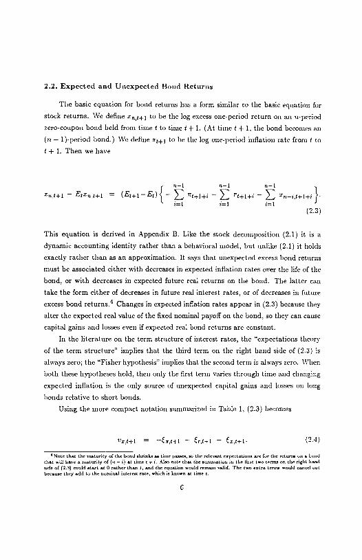
2.2. Expected and Unexpected Bond Returns

The basic equation for bond returns Isas a form similar to the basic equation fur

stock returns. We define Xnf+1 to be the log excess one-period return on an n-period

zero-coupois bond held from time I to time I + 1. (At time I + 1, the bond becomes an

(n — 1)-period bond.) 'We define lrtH to be the log one-period inflation rate from ito

1+1. Then we have

— Ejxt+i = (Et+i _E){ — ri+t+i — rt+1+1 —

}•

(2.3)

This equation is derived in Appendix B. Like the stock decomposition (2.1) it is a

dynamic accounting identity rather than a behavioral model, but unlike (2.1) it holds

exactly rather than as an approximation. It says that unexpected excess bond returns

must be associated either with decreases in expected inflation rates over the life of the

bond, or with decreases in expected future real returns on the botsd. The latter cantake the form either of decreases in future real interest rates, or of decreases in future

excess bond returns.4 Changes in expected inflation rates appear in (2.3) because they

alter the expected real value of the fixed nominal payoff on the bond, so they can cause

capital gains and losses even if expected real bond returns are constant.

In the literature on the term structure of interest rates, the "expectations theory

of the term structure" implies that the third term on the right hand side of (2.3) isalways zero; the "Fisher hypothesis" implies that the second term is always zero. \Vhen

both these hypotheses hold, then only the first term varies through time and changing

expected inflation is the only source of unexpected capital gains and losses on long

bonds relative to short bonds.

Using the more compact notation summarized us Table 1, (2.3) becontes

Vx,t+1 = e,r,t+i —Cr,t+1

— (2.4)

Note that the maturity of the hood shrinks as time pasnes, so the relevant eopertations are for the retorm on a hoodthat wi5 have a maturity of (n — i) at time t + i. Also note that the summation in the fust two terms ow the right handside of (2.3) mold start at 5 rather than 1, and the eqoation woold remoiw valid. The two entra terms ,noald ranmel oathemaose thvy add to the oomioal interest rate, whioh is hnown at time t.

—6—

2.3. Asset Prices, Yields, and Returns as Forecasting Variables

Several authors have recently found that long-term asset prices can be surpris-

ingly powerful forecasting variables. Prices are sometimes used in raw form, but more

commonly they are used as elements of asset yields or yield spreads. For example,

Campbell and Shiller (1988a,b) and Fama and French (l9SSb) use dividend yields to

forecast stock returns, while Campbell and Shiller (1991), Fama (199Db) and Mishkin

(1990) use bond yield spreads to forecast future bond returns, interest rates and infla-

tion rates. The forecasting power of asset price variables is particularly evident when

forecasts are made over long horizons. The asset pricing framework descril,ed above

can be used to interpret these findings.

The approximate log-linear asset pricing framework for stocks implies that the real

stock price p embodies investors' forecasts of future real dividends, real interest rates,

and excess returns on stock. Appendix A shows that

= E [(1 —p)d11 — — +i+1, (2.5)

where a constant term has been suppressed since it plays no role in our analysis. It is

often argued that real dividends follow a time series process with a unit root (Klcidoii

1986). Equation (2.5) shows that a unit root in real dividends will lead to a unit rootin stock prices; this will cause econometric problems if stock prices arc used to forecast

stationary variables. In this case one might want to work with the log dividend-price

ratio or dividend yield, which satisfies

dg —pg = E + + (2.6)

The log dividend yield is stationary if dividend growth rates, real interest rates, andexcess stock returns are all stationary. As we discuss further below, in our data setthese conditions appear to be met.

Equation (2.6) helps to explain why the dividend-price ratio has forecasting powerfor excess stock returns at long horizons. The third term on the right hand side of

—7—

(2.6) is approximately equal to the conditional expectation of the long-horizoo excess

return.5 Provided that the other two terms on the right hand side of (2.6) are not too

variable, the dividend-price ratio should perform well as a proxy for the long-horizon

expected excess return. More generally, if there is any variation io the expected excess

return, the dividend-price ratio should have some forecasting power.6

A similar point can be made for bonds, without the use of any log-lioear approxi-

mation. In the case of bonds, it is conventional to begin by transforming nominal Prices

to yields to maturity. The nominal log yield to maturity, y,i,, is minus the nominallog bond price divided by n. Appendix B relates the nominal bond yield to expectedfuture real bond returns and inflation rates:

= (!) E1 [rg+i+1 + rt+l+j + x_,g+t+]. (2.7)

Inflation rates take the place of real dividends in the bond analysis. Just as with real

dividends, it is often argued that inflation rates follow a nonstationary unit root process.

In this case the nominal bond yield will also be nonstationary and one may want to

work with a yield spread instead of the yield itself. The yield spread between the ii-period nominal interest rate and the 1-period nominal interest rate, 3j w,t — I/il,can he written as

= [(n — 1 — i)(Tg2j + Ar1÷2) + x_j . (2.8)

The yield spread is stationary if excess bond returns, inflation changes, and real interest

rate changes are stationary. In our data set these conditions appear to be met.

Equation (2.8) relates nominal yield spreads to expected future changes in infla-tion rates and real interest rates, and to expected excess returns on long bonds. The

expectations theory of the term structure makes the third term on the right hand side

Cazephell and 5hiller (lsssb) esepliazixe this poiot.This will fail only if the long-horizon expected exox return is perfectly ,srgatively correlated with some other con,po-

neat of the dzvsdmsd yield, nod these too components have exactly the right vo.riosces so that their voriotioe oaecels ootof the divideed yield.

—8—

of (2.8) constant, while the Fisher hypothesis makes the second term on the right hand

side zero. These hypotheses are extreme. In general, the nominal yield spread willbe a useful proxy for expectations of all the terms on the right hand side. This helps

to explain why yield spreads help to forecast long-horizon movements in inflation and

interest rates, as well as excess returns on long bonds.7

An alternative way to forecast asset returns is to use the history of asset returns

themselves. This univariate approach was popular in the early empirical finance liter-

ature; more recently it has been used by Fama and French (1988a) and Poterba and

Summers (1988), who emphasize that one should look at the entire autocorrelation func-

tion of returns. Specifically, there may be negative autocorrelation at low frequencies

which makes long-horizon lagged returns better forecasters than short-horizon lagged

returns. Poterba and Summers argue that "If market and fundamental values diverge,

but beyond some range the differences arc eliminated by speculative forces, then stock

prices will revert to their mean. Returns must be negatively serially correlated at some

frequency if 'erroneous' market moves are eventually corrected" (pp.27-28).

Campbell (1991) uses the asset pricing framework developed above to clarify the

circumstances under which univariate regressions will have forecasting power for re-

turns. Campbell studies a simple example in which the expected stock return follows

a first-order autoregressive process. He shows that persistent movements in expected

returns have offsetting effects on the autocorrelations of realized returns. On the one

band, the positive autocorrelations of expected returns carry over to realized returns;

on the other hand, the capital loss associated with an increase in the expected re-turn creates negative autocorrelations in the realized return series. These offsetting

effects make it possible that all the autocovariances of stock returns are zero, even

when expected returns are variable and persistent. Contrary to the claim of Poterba

and Summers, time-varying expected returns do not necessarily imply negative (orpositive) autocorrelations at any frequency.

Of course, in practice it is unlikely that realized stock returns will have autocovari-

ances that are all exactly zero. Campbell's example simply shows that autocovariances

may bc close to zero even when changing expected returns contribute a great deal to the

cx posi variability of returns. Thus lagged returns may be less effective than dividend

yields and other price-based variables in forecasting future returns.

'Estrnlin nod Lfnrdoovnlit (1991) nod Stodt nod Vntnon (1990) nhow th.tt yinld nprnndo wino hoip to forncnt tho nodocooonon oia.vity. Equntion (2.8) nhoold bo Itoiplul in thinking nbout why thin in no.

—9—

2.4. Level Portfolios and Slope Portfolios

In studying the properties of bond returns, it is common to distinguish between

returns that are associated with changes in the general level of interest rates, andreturns that are associated with changes in long-term interest rates relative to short-

term rates (shifts in the slope of the term structure). In fact, theoretical bond pricing

models often assume that there are two "factors" driving interest rates which can he

associated with shifts in the level and slope of the term structure.

Our variance decomposition approach is perfectly consistent with this way of think-

ing about bond returns. We now show that the excess return on an n-period bond can

be written as the sum of excess returns on two portfolios, a "level portfolio" of 2-period

bills whose excess return 'n,t+l is sensitive only to innovations in the level of short-term

nominal interest rates, and a "slope portfolio", long in n-period bonds and short in 2-

period hills, whose excess return m,+1 is sensitive only to changes in the yield spread

between long rates and short rates. The returns on the level and slope portfolios can be

broken into components in just the same way as excess bond and stock returns. These

decompositions answer the questions "What moves the short-term nominal interest

rate?", and "What moves the slope of the term structure?", respectively.

The excess return on an n-period bond can trivially he written as

= 1n,t-4-1 + mng+1, (2.9)

where the components 1nt+1 and mn,j+1 are defined by

(n —

Xn,t+j — (n — l)'2,t+I. (2.10)

It is straightforward to show that the unexpected return on the n-period bond is—(n — 1) times the innovation in next period's yield on the bond, wlnle the unex-pected return on the level portfolio is —(n — 1) times the innovation in next period's

short-term interest rate and the unexpected return on the slope portfolio is —(n — 1)

— 10 —

times the innovation in next period's yield spread. It follows from this (or from equa-

tions (2.3) and (2.10)) that the level and slope portfolio returns can be decomposed as

follows:

'n,t+I — = — (n — 1)(Et÷i — E1) Nrt-÷2 + rt+2],

— E1 mnj+1 =

n—I— (E+j — E) [(n — 1 — )(t+2+j + r1÷21) + (2.11)

1=1

In our more compact notation, (2.11) becomes

—A,i+i —

Vm,t+1 = Pw,1+l Pr,t+1 — /2z,1+I• (2.12)

These equations say that level portfolio returns are driven by changing expecta-tions of inflation and real interest rates one period ahead. Slope portfolio returns are

determined by changing expectations of longer-term changes in inflation and real in-tcrest rates between the next period ahead and the more distant future, and also by

changing expectations of future excess returns on long-term bonds. In our empirical

work, the distinction between these portfolios turns out to be important. Our variance

decomposition for bond returns places little weight on news about future real inter-

est rates, but real interest rate variability is important for both the level and slope

portfolios considered separately.

- 11

3. Alternative Methods for Empirical Variance Decomposition

In the previous section we have stated a nunsber of identities relating innovations

in long-term asset returns to revisions in investors' expectations of future dividends,

real interest rates, inflation rates, aud excess long-term asset returns. Our objective is

to use these identities to estimate the relative importance of the different componentsfor the historical behavior of asset returns.

In this section we first discuss some conceptual difficulties with the decomposition

of return variance when the components of returns are correlated witis one another.

We then address the question of how one can form empirical proxies for revisioxss in

expectations. We discuss the contemporaneous regression approach to this problembefore introducing our preferred vector autoregressive method.

3.1. Variance Decomposition with Correlated Components

For concreteness, we consider the decomposition of excess stock returns. We begin

with the identity (2.2), which we restate here:

= d,t+1 — r,t+1 — (3.1)

For the present we will assume that the components 5d,t+1' 5r,t+1, and 5e,t+1 are directlyobservable; below we discuss tlse difficulties that arise from the fact that the components

are unobservable.

In general the components in (3.1) can be correlated with each other. This creates

a conceptual difficulty in stating a variance decomposition for °ci+1 Trivially we have

Var(ve,+i) = Var(cdt.÷j) + Var(r,e+j) + Var(c5,t+i)

— 2 Cov(ed 1+1, r,t+i) — 2 Cov(cd,j+l, Q+i) + 2 Cov(er,t+j, Q,i+1) (3.2)

One way to state a variance decomposition is simply to report the six numbers on the

right hand side of (3.2), and we do this in our empirical work below. A number like

— 12 —

Var(Sd,j+l) answers the question, "What would the variance of stock returns be if the

process for stock dividends remained unchanged, but interest rates and expected excess

stock returns became constant?". Whether this question is meaningful depends on the

context. In an exchange economy, for example, stock dividends are modelled as an

exogenous endowment while interest rates and expected excess stock returns depend

on the dividend process and on the risk aversion of a representative agent. In such an

economy one could imagine reducing the risk aversion of the representative agent to

zero, while leaving the endowment process unchanged. The effect of this would be to

change the variance of stock returns to Var(fdj+I).

Alternatively, one may want to transform the components in (3.1) so that they arc

orthogonal to one another. Var(ve,t+i) can then be written as a sum of variances of the

orthogonalized components. One simple and popular way to orthogonalize componentsis to order them and then apply a Cholesky decomposition. The variance of the first

component in such an ordering is given by the variance of the fitted value in a simple

regression of Vg+1 on that component.It is tempting to think that a component will have the largest share of variance

when it is given first place in the ordering, in other words that the R2 statistic ofa simple regression of v+1 on a component will be an upper bound on the variance

share of that component. Unfortunately this is incorrect. It is possible for a component

to have a larger share of variance when it is placed lower in the ordering. To see this,

note that if one component is negatively correlated with the others then it can beuncorrclated with the sum of the components. This component will get a zero share of

variance when it is ordered first, but in general it will get a nonzero share when it is

given a lower place in the ordering.8 Despite this difficulty of interpretation, a popularnieasure of the importance of a component is the 2 statistic from a simple regressionon that component. Accordingly we report this measure in our empirical work below.

Although correlation among components leads to ambiguity in the notion of a

variance decomposition, this does not mean that the decomposition summarized by

(3.1) and (3.2) is uninteresting when the components arc correlated. The observation

that the various components of an asset return are highly correlated may itself be an

important stylized fact.

'Below we show that thin in not j,ist a theoretical possibility, but occurs in sOme of our sort return decompositions.For similar reasons the sum of the flt statistics from simple regressions on all the individual components may be eithergeento- or less than one, which would be the R2 from a mulLiple regreonon on the romponents.

13 -

3.2. The Contemporaneous Regression Approach

In practice the expectational revisions in equation (3.1) are not directly observable.

Cutler, Poterba, and Summers (1989), Fama (1990a), and Stainbaugh (1990) have used

contemporaneous regressions to deal with this problem. As we noted above, a popular

measure of the importance of a particular component is the variance of the fittedvalue obtained when Ve,t.4.1 is regressed on that component. The contemporaneousregression approach uses instead a vector of explanatory variables w4 that proxiesfor the unobserved component. For concreteness, assume that wt+l is supposed to be

a proxy for dt+1• The following ordinary least squares (OLS) regression is run:

= I9'w+i +77+I. (3.3)

Then the variance of the fitted value of (3.3) is taken as a proxy for the variance ofthe fitted value of a regression of v1 on The condition for this to be valid,of course, is

Var(E[ve,i+i wt+1 = var(ELvt+i Ied,1l-I i) (3.4)

A sufficient condition for (3.4) to hold is that

E[ve,i+iiwt+i] = E[ve,+1kd+l1. (3.5)

Equation (3.5) is of course not necessary for (3.4), but we focus on this conditionbecause it is hard to construct plausible examples in which (3.5) fails but (3.4) holds

(other than by an unlikely coincidence). The condition (3.5) is in fact a fairly stringent

one. To sec this, note that (3.5) is not necessarily satisfied even if the vector is a

perfect proxy for d+I in the sense that d,g+1 can be written as a linear combination

of the variables in wg+1:

d,1+1 = (3.6)

— 14 —

for some vector 0. Even when (3.6) holds, it could be the case that the other components

of v 8+1 can also be written as linear combinations of the variables in wj+1. For this

or other reasons the vector w1. may contain more information about Vet.I than does

the single component dt+l9Finally, we note that the contemporaneous regression approach can at best provide

an estimate of the share of variance attributed to a component when it is ordered first

in a process of sequential orthogonalization. This is not even an upper bound on the

share of variance that can be attributed to the component, because other positions in

the ordering might give the component a larger share of variance. Thus the information

that can be obtained from the contemporaneous regression approach is quite limited.

3.3. The Vector Autoregressive Approach

The vector autoregressive (VAR) approach is more ambitious than the contem-

poraneous regression approach in that it seeks to use the time-series structure of the

problem to identify revisions in expectations. The VAR approach postulates that theunobserved components of returns can be written as linear combinations of innovations

to observable variables: that is, equations like (3.6) hold for each of the components

of returns. The coefficients in these linear combinations are identified by using a time-

series model to construct forecasts of the discounted value of future dividends, realinterest rates, excess returns, and so forth. Revisions in these forecasts are then used

as proxies for revisions in investors' expectations. This approach must confront twoproblems. First, the relevant expectations are of variables that are realized only over

very long periods of time. (In the case of stocks, in fact, the expectations concern theinfinite future.) Second, investors may have information that is not available to us.

We handle the first problem by using a VAR model to calculate multi-periodexpectations. In effect, we use the short-run behavior of the variables to impute the

long-run behavior. This procedure seems to have better finite-sample properties than

direct regression methods with long-horizon variables, although of course it is necessary

to assume that the VAR adequately captures the dynamics of the data. 10

Note that even when (3.5) nod (3.6) hold, the OLS regression coefficients P in (3.3) will not genveslly equal thepss-nmemn 8 in (3.6). Equality of P nod 8 would reqoire io oddition that ea,. be orthogonal to She otltee components of"its'-

loVA are used by Campbell nod Shiller (1987, 1988.,b) nod Kaizdel and Siasnhaugh (1988). Pama sod Frendi(1988a,b) pioneered the use of long-horizon regressions. The finite-sample properties of such regrenstons are investigatedby Riclasrdson nod Stodi (1989) and Ilodrich (199!); Hodrivk explicitly compares them with VAR procedures. Ca,npbefl(1991) also ,,rnlertakes a Monte Carlo eoly of the properties of VAR vnsisxce decompositions.

— 15 —

The second problem is snore difficult. In general there is no way to rule out the

possibility that investors may have information, omitted from our VAR, which affects

the decomposition of variance. A special case where investors' superior information

causes no problem occurs when only one component of an asset price is time-varying.

In this case the asset price itself summarizes all the information investors have about

that component (Campbell and Shiller 1987). Thus if one is interested in testing the

hypothesis that expected real interest rates and excess returns on long bonds are con-stant, this can be done using a VAR that includes the long bond yield or yield spread;

under the null hypothesis the yield varies only because expected inflation varies, soit embodies all the relevant information about inflation that investors possess. When

several components of an asset price are variable, however, the asset price will be an

imperfect proxy for investors' information about any one component. In this case theVAR results must be interpreted more cautiously, as giving a variance decomposition

conditional on whatever information is included in the system. In practice it seemslikely that the VAR results will tend to overstate the importance of wluchever compo-

nent is treated as a residual, but the sign of the bias will depend on the covariancesbetween omitted and included variables.11

The VAR approach begins by defining a vector of state variables that help tomeasure or forecast excess returns. These variables are chosen to be stationary, and

for notational convenience we treat them as having zero means. (In our empirical work

we remove sample means from all variables beforc estimating the VAR process.)

In order to measure excess returns and their components, our state vector must

include at least the excess stock return, the real interest rate, the change in the nominal

interest rate, and the long-short yield spread. In addition we use other variables thathave been shown to forecast excess bond and stock returns, real interest rates, and

inflation rates. These variables are the dividend-price ratio, the 2-period yield spread,

and the "relative bill rate". The relative bill rate, which is given further motivation

below, is defined as the level of the short rate relative to a 1-year backwards moving

average of short rates, or equivalently a.s a triangular 1-year moving average of changesin short rates. Ve use the notation rbj for the relative bill rate, where

" This potential prob5nes of omitted information him is of cooree shared by the contemporaneom regression approach.

- 16 -

rb1 Y1l — ()12

= (1 — (3.7)

Writing :g for the state vector and making the relative bill rate the last element,

we have

= [e1, r, Y1,t, 8,g, d1 — p, S21, rbj]'. (3.8)

Next we assume that the state vector follows a first-order VAR process:

zl+1 = Az1 + (3.9)

The matrix A is the coefficient matrix of the VAR, and wg is the error vector. The

assumption that the VAR is first-order is not restrictive; higher-order VAR models arc

handled by augmenting the state vector and reinterpreting A as the companion matrix

of the system. We also define vectors ci through e4 as the four columns of a 4 x 4identity matrix. The vector ci is used to pick out the i'th element of the state vector.

Innovations to excess returns can now be obtained directly from the VAR error

vector. We have Vet+1 = ci'wj+i simply from the fact that ej is the first element of

the state vector. The remaining innovations satisfy vzl÷I = —(n — i)(e3' + e4')wj+i,= —(n — 1)c3'wt+i, and Vmg+1 = —(n — 1)e4'wt÷i. These expressions

follow from the facts that the unexpected slope portfolio return is —(n — 1) times

the innovation in the yield spread, the unexpected level portfolio return is —(n — 1)

times the innovation in the short-term nominal interest rate, and the unexpected bond

portfolio return is the sum of the unexpected slope and level portfolio returns.12 To

obtain VAR estimates of revisions in long-horizon expectations, we use the fact that

(Et+j — E1)z1 = .42w1+i. (3.10)

IS These formulas use the fact that the innovaLion in the level of the short rate in the same as the innovation in the changeof the short rate. since invtors know the lagged short rate level beforehand. Also we ignore the distinction between os.,and This introduces an approtintat ion error that is very small alien it is 1argv.

- 17 -

Tins can be used to calculate eacil of tIle components of portfolio returns as a linear

combination of the elements of the shock vector u't+l.

For stock returns, we obtain the coloponents s and r by forecasting excess stock

returns and real interest rates respectively, while the remaining componeot 5d is ob-

tained from (2.2) as a residual. We give details of this procedure, which follows Camp-

bell (1990a, 1991), in Appendix C. One could instead include dividend growth rates in

the vector zj, leaving some other term to be the residual. However this would have two

important disadvantages. First, monthly dividends display seasonal variation, whichwould need to be handled as part of the forecasting procedure. Second, there is some

doubt as to whether dividends follow a linear time-series model with constant coeffi-

cients.13

For bond returns, we first note that the change in inflation can be obtained from the

elements of the state vector as itj.j= yi,t— rt+1, so the innovation in the change

in inflation and the innovation in the cx po.st real interest rate both equal —e2'wj+j.

One component of the excess bond return is a sum of revisions in expected inflation

levels, but this can be rewritten as a weighted sum of revisions in expected inflation

changes. We obtain inflation and real interest rate components by direct forecasting,

leaving the revision in expected excess returns as the residual. This choice of residual

is forced on us because we cannot directly measure the sequence of excess returns on

the bond as its maturity shrinks over its remaining life. The components of slope and

level portfolio returns are calculated in the analogous mnnner to the components of

bond returns. The formulas for these components are given in Appendix C.

The one remaining issue to address is how we calculate standard errors for statis-

tics such as the variance of a particular component of returns. Our approach is totreat the VAR coefficients, and the elements of the variance-covariance matrix of VAR

innovations, as parameters to be jointly estimated by Generalized Method of Moments

(Hansen 1982). The 0MM parameter estimates are numerically identical to standard

OLS estimates, but 0MM delivers a heteroskedasticity-consistent variance-covariance

matrix for the entire set of parameters (White 1984). Call the entire set of parameters

y, and tlse variance-covariance matrix V. Consider a statistic such as the variance of

iSThe Modigliaro-Miller propositimis on the irrelevance of dividend policy give no no tlteoretioal reason to expert man-agero tn parson any particular dividritd policy. Some have argued that this ondennines eiopiriral work that appliesstandard time-serim methods to dividends. Lelitnano (1991), for rnaniple, snys that "Time cnnventionnl practice nfasoum-ing a particular dividend policy nod computing its prvsent value is Iratiglit with haoatvl.... Thvreisnohistantial reason tnhelieve that any aaoomed dividend policy is nosspvrised since nianagers have no ohciros iocvntive tv adopt or maintain aconsistent dividend policy.' (pt). Whatever the merits of Leltmaon's arg'aoent, it does not apply herr siitce our appmadiones no information on the timing of dividend paymei,io ao opposed to their presevt valor.

— 18 —

news about future excess stock returns relative to the variance of unexpected stock re-

turns. This can be written as a nonlinear function f(y) of the parameter vector y. Then

we estimate the standard error for the statistic in standard fashion as

— 19 —

4. An Application to Postwar U.S. Data

4.1. Data and Sample Period

We now apply our methods to postwar U.S. data on stock and bond returns. Our

stock index is the value-weighted index of stocks traded on the NYSE and AMEX, as

calculated by the Center for Research in Security Prices (CRSP) at the University ofChicago. We measure the dividend yield on the index in a standard fashion, taking

total dividends paid over the previous year relative to the current stock price.

For nominal interest rates, we use McCulloch's (1990) data set on zero-coupon

yields implied by the yield curve for U.S. Treasury securities. At maturities beyond

one year, U.S. Treasury securities pay coupons so McCulloch uses a cubic spline method

to calculate an implied zero-coupon yield curve. The McCulloch data are available at

the beginning of each month from 1947:1-1987:3, but we start our sample in 1952:1 in

order to avoid the period before the 1951 Treasury-Fed Accord. We set n, the maturity

of our long bond, equal to 10 years (120 months) as this is the longest maturity that

is available throughout the sample period.14

Our flisal piece of data is a price index for deflating nominal asset returns. We use

the Consumer Price Index, adjusted before 1983 to reflect the improved treatment of

housing costs that is used in the official index only after 1983.

Throughout the paper we report results for the full sample period 1952:1-1987:2,

as well as for subsamples 1952:1-1979:9, 1952:1-1972:12, and 1973:1-1987:2. The first

of these subsamples is chosen to exclude the period after the change in Federal Reserve

operating procedures in October 1979. The level and volatility of interest rates in-

creased considerably during the 1979-82 period, and it may be unreasonable to impose

a constant linear time-series model on the pre- and post-1979 data together. The sec-

ond subsample is chosen because it lsas been argued (Faina 1975) that the real interest

rate was constant during the 1950's and 1960's; this would imply that all movements in

nominal interest rates during this period were due to changing expectations of fnture

inflation (and perhaps term premiums on longer-maturity bonds). The third subsampleis the complement of the second subsample.

Table 2 reports some basic sumsoary statistics about the second moments of excess

0Cunipbdll and 5hilln (Issi) also use mite MoCulloch dots The main altanative nero-coupon yield series is due toEugene Fama and Robert Bliss and is available (ruin CR5!'. This alternative baa the advanbsge that it is avaliuhie up tuthe present, but the dinadvantage that the longat maturity is See yearn.

— 20 —

returns on stocks, 10-year bonds, the level portfolio (2-month bills), and the slopeportfolio (long in 10-year bonds, short in 2-month bills). All excess returns are measured

monthly over the return on a 1-month Treasury bill. For each sample period we report

variances and covadances (on and below the diagonal) and correlations (in bold face

above the diagonal).

The main results iii Table 2 are as follows. Looking first at the variances of excess

returns, we see that stock returns are more volatile than 10-year bond returns but the

difference in variance is much larger in the early part of the sample. In 1952-72, thestock variance is about 4 times as large as the bond variance, whereas in 1973-87 the

difference in variance is less than 10%. It is also noteworthy that both the level and

slope portfolios have higher variances than 10-year bonds; below we interpret this fact.

As for the correlations, the most striking feature of Table 2 is the very low cor-

relation between excess returns on stocks and bonds. Conventional wisdom is that

long-term asset prices move (or should move) together, but the monthly correlationbetween stock and bond returns never exceeds 0.075 in any sample. The correlations

between stock returns on the one hand and level and slope portfolio returns on theother are also very close to zero. However the level and slope portfolio returns have a

very strong tendency to move in opposite directions, with correlations lying between-0.85 and -0.90 in every sample. This reflects the fact that long-term interest rates aresmoother than short-term rates, so an increase in short-term rates (a negative return

on the level portfolio) tends to be associated with a decline in the yield spread (a pos-

itive return on the slope portfolio). The negative correlation between level and slope

portfolios also explains why these portfolios each have higher variances than the bond

portfolio, which is their sum.

The next step in our analysis is to run the VAR system described inthe previous

section. This system includes seven variables: the excess stock return, real interest

rate, change in the nominal 1-month interest rate, and 10 year-i month yield spread,

which are needed to measure returns and their components; and the dividend-price

ratio, 2 month-i month yield spread, and relative bill rate, which are useful forecasting

variables. The main variable that may need some discussion is the relative bill rate.This is defined to be the current i-month bill rate, less a backwards 1-year moving

averagc of bill rates. Equivalently, it can be described as a triangular 1-year moving

average of past changes in bill rates. The relative bill rate helps to capture some of

the longer-run dynamics of changes in interest rates without introducing long lags, and

— 21 —

hence a large number of parameters, into the VAR system. 15

All the variables in the VAR system appear to be stationary in our sample period.

Dickey-Fuller tests and augmented Dickey-Fuller tests with 4 lags reject the unit roothypothesis at the 5% level or better for each series included in the VAR.16

The number of variables in the VAR increases very rapidly with the lag length, so

there is some danger of overfitting when a high-order VAR is used. For this reason we

report results from a parsimonious first-order VAR in the full sample and all subsam-

ples. We also give results from a third-order VAR estimated over the full sample, toshow that our findings are robust to VAR lag length.17

4.2. Variance Decompositions for Excess Bond and Stock Returns

In Tables 3 and 4 we report the variance decompositions implied by the VAR for

excess stock and bond returns, respectively. The first row of each table shows the 2when the VAR is used to forecast the monthly excess return on stocks or bonds, along

with the joint significance level of the forecasting variables. Then the tables report the

variances and covariances of the different components of the portfolio returns. These

are normalized by the variance of the return innovation itself so the numbers reported

are shares that add up to one. Finally the tables show the implied 1?2 statistics thatwould be obtained in simple regressions of the unexpected excess return on each of the

estimated components. As discussed above, these R2 statistics are alternative measures

of the importance of components. The variance and cnvariance shares and implied R2

statistics of the components are reported witls asymptotic standard errors, reflecting

the fact that the components are not directly observed but are estimated from a VAR

system.

Table 3 gives a variance decomposition for excess stock returns, similar to the one

reported in Campbell (1991). The fl2 for forecasting excess stock returns at a monthly

frequency is quite modcst: just over 5% for the full sample, although it is somewhat

The relative bill rate is atno used by Campbell (lana, IssI) and ilodrick (1991).n Haraky and neLong (1989) argue that the dividend growth rate may have a unit root, which would put a unit root

in the dividend-proc ratio. however there is very little direct evidence for this proposition; Haeehy and neLong arguefoe it on the grounds that unit root tests may falsely reject the null hypothmenis in finite oncoplee. II ore we use mmit roottests to indicate whether atatieoary soynmptotio distributions are likedy to ho a good appronimatico to the flnite-aampledietrihotices of VAR coracionte and tent statieties.

Over the foil na.,ople, a Womd teet for joint significance of time seccmni lag variables when these ace added to the first-order VAR provides umrcog ecidence tlmatanecnnd lag should be included. Timers is weaker evidence for a third lag; thetiord lag variables ace icmmmtly significant at the s% level only in time forennucing rqoatinn for time dicidend-price ratio. Wealso calculated variance decosnpoaitiono for a sin-lag VAR, which were similar to those reported.

— 22 —

higher in the subsamples.18 The joint significance of the forecasting variables is 0.1%in the full sample, and less than 0.1% in the earlier subsamples. In the 1973-87 period

the forecasting variables narrowly fail to be significant at the 10% level.

Despite the modest degree of forecasting power for stock returns, the full sample

variance decomposition attributes less than 15% of the variance of stock returns to

the variance of news about future dividends, and almost 75% to the variance of news

about future excess returns. The decompositions for subsamples are fairly similar; the

variance of news about future dividends is never more than 25% of the variance ofexcess returns, while the variance of news about future excess returns is never less

than 60% of the variance. Simple regressions of unexpected excess stock returns on the

estimated components show a similar pattern. In the full sample, news about future

excess returns can explain (in the sense of least-squares regression) more than 85% of

the variance of unexpected excess stock returns, while news about future dividends

explains less than 15% of the variance. Across subsamples, news about excess returns

never explains less than 79% and news about dividends never explains more than 42%of the variance.

At a mechanical level, the reason why excess return news plays such an important

role is that changes in expected excess returns are highly persistent. Thus modest

movements in short-run expected returns are capitalized into large changes in stock

prices. The persistence of expected returns arises from the persistence of the dividend-

price ratio, which is an important forecasting variable for excess stock returns. This

point is discussed in greater detail in Campbell (1990a, 1991).News about real interest rates plays a relatively minor role in the variance decom-

position for stock returns. This is particularly true in the earlier subsamples, 1952-79

and 1952-72. In these sample periods the er p03i real interest rate is hard to forecast.

The R2 for the VAR's real interest rate equation (not reported in the table) is only 5%

in 1952-79, and 6% in 1952-72.' This lack of forecastability means that the variances

and covariances involving real interest rate news are tiny and precisely estimated, while

the R2 statistics for simple regressions of stock returns on real interest rate news are

1% in the period 1952-79 and 3% in 1952-72.

In the late 1970's and 1980's the real interest rate becomes more forecastable, with

' To tome rottot of 000e,e the relatively hi5I, R2 ntnli.tkn in .b.tnpkn reflect overfitting in .maller dnt. tot..° Even o thvne narople period, the torecting vno-ialrle, are jointly nigni&aot for the real lntmeut rate at the 5% level,

,ndrrroting that the or note real intervot rote it not literally 0000tont. Thin contranti with Fooxa'. (197s) finding. Theres,iIts here are booed on a large information set and use a different price index, which may account for the diffaence in

— 23 —

112 statistics (not reported in the table) of 20% in 1052-87 and 46% in 1973-87. Even

here, however, real interest rate variation is largely transitory; it does not cumulate

over time in the way that changes in expected excess returns do. Thus the variance of

real interest rate news remains small in all our sample periods. There is however an

imprecisely estimated positive covariance between real interest rate news and excess

return news in the later subsamples. This covariance is attributed to the independent

variable in a simple regression of unexpected stock returns on real interest rate news,

so the simple regression 112 is over 20% in our sample periods that include the 1980's.

Table 4 presents a VAR analysis of excess bond returns. The results have some

similarities with the results for stock returns, but also some interesting differences. The

monthly forecastability of excess bond returns is similar to the forecastability of stock

returns over the full sample, with an fl2 of 5% and a joint significance level of 0.2%.

However the forecastability of bond returns comes from the post-1973 or post-1979

data rather than the earlier data. This is the opposite pattern from Table 3, whichshowed that stock returns are more forecastable in the earlier subsamples.

In the subperiods 1952-79 and 1952-72, the variance decomposition for bond re-

turns can be described very simply. Almost all the variation in bond returns over this

period can be accounted for by news about future inflation, while the other components

are small and imprecisely estimated. The variance of inflation news is insignificantly

different from the variance of unexpected excess bond returns, and a simple regression

of bond returns on inflation news yields an 112 insignificantly different from one.

In the sample periods that include 1980's data, the story is somewhat more com-

plicated. Inflation news is still the dominant component of bond returns, whether one

looks at variance shares or 112 statistics from simple regressions. But now there is some

variation in news about future excess returns on bonds, and it appears to be negatively

correlated with news about future inflation. In words, this means that when investors

learn that long-run inflation will be higher than they expected, they also tend to learn

that excess bond returns will be lor than they expected. This has the effect of de-

creasing bond price variability because the capital loss from higher expected inflationis partly offset by a capital gain from lower expected excess bond returns. It shouldbe kept in mind, however, that the terms involving excess bond returns in Table 4 are

extremely imprecisely estimated.

- 24 —

4.3. A Covariance Decomposition for Excess Bond and Stock Returns

In Tables 5 and 6 we study the determinants of the covariance between excess stock

and bond returns. Table 5 reports the correlation matrix of the return componentsand , estimated from a 1-lag VAR over the full sample and each of

our subsamples. The first row of Table 0 gives the covariance between the stock return

innovation u and the bond return innovation V. This is always close to zero, as one

would expect from the covariances of the raw excess returns reported in Table 2. The

lower panels of Table 6 show the covariance of t'e with each of the components of tj,

and the covariance of vz with each of the components of v. Thus Table 6 answersthe question, "What would be the covariance of bond and stock returns if one of these

asset returns consisted of a single component while the other return were as measured

in the data?".We can now see some of the reasons why the covariance of excess stock and bond

returns is so small. In our earlier subsainples 1952-72 and 1952-79, the excess stockreturn has small covariances with all the components of the excess bond return. In this

period stocks do not seem to be negatively affected by long-run increases in inflation,while expected real interest rates and excess bond returns are not very variable.

When we include data from the 1980's, there appear to be offsetting effects. The

excess stock return covaries positively with news about future inflation , but nega-tively with news about future real interest rates r and news about future excess bond

returns . The negative correlation between the excess stock return and the bond

return component is due largely to a positive correlation between news about future

excess stock returns 5e and news about future excess bond returns shown in Table

•2O In any event, the positive inflation covariance tends to offset the negative real

interest rate and excess return covariances, leaving the overall covariance close to zero.

4.4. Variance Decompositions for Level and Slope Portfolio Returns

Further insight into these results can be gained from Tables 7 and 8, which decom-

pose the variances of returns on level and slope portfolios. The only two components

of returns on the level portfolio of two-month bills arc the news about inflation and

real interest rates one month ahead. Table 7 shows that these two components have a

'° F.ssno ocsd Frenth (1989) emphaxire thi. positive correlation smons eapocted reture. on differeesi long-term axaxt.. Wenote howev,r that our estimate. of Con(e,, ,) ,,ever exceed 0.4.

— 25 —

strong tendency to offset each other. The variances of both news components exceed

the variance of the level portfolio rotorn, but they have a large negative covariance.

This reflects the fact that short-run forecasts of inflation and real interest rates are

negatively correlated. A positive innovation in expected inflation tends to be associ-

ated with a negative innovation in the expected real interest rate, so that the effect on

the short-term nominal interest rate is dampened.

Table 7 also illustrates the point, discussed as a theoretical possibility in section

(3.1), that a variable component of an asset return can have almost no explanatorypower in a simple regression of the return on that component. According to Table7 short-term real interest rate variation is important and tends to offset short-termvariation in inflation, but because inflation news dominates the level portfolio return

the explanatory power of real interest rate news in a simple regression is negligible.21

The pattern of results in Table 7 is very striking, but for two reasons it should be

interpreted with some caution. First, in the earlier subsamples 1952-79 and 1952-72

the real interest rate terms are not significantly different from zero and the varianceshare of inflation news is not significantly different from one. This reflects the weak

forecastability of or post real interest rates in this period. Second, forecastable mea-

surement error in inflation might create the pattern of results in Table 7 even in aworld in which true real interest rates were constant. Measurement error is unlikely to

be the whole explanation, however, as numerous authors have recorded the opposing

low-frequency movements of inflation and real interest rates in the late 1970's and early

1980's.

Table 8 gives a variance decomposition for the excess return on a slope portfolio,

long 10-year bonds and short 2-month bills. Here again we find an important role for

forecasts of both inflation and real interest rates, now measured as changes from a one-

month horizon to a ten-year horizon. Just as in Table 7, innovations in these forecasts

of inflation and real interest rates have a tendency to offset each other. Each considered

in isolation implies a more variable portfolio rcturn than we observe, but they have a

strong negative covariance which tends to reduce the variability of the slope portfolio

return.

It may seem puzzling that real interest rate variation plays an important role forlevel and slope portfolio returns but is much less important for the excess bond return,

winch is the sum of the level and slope portfolios. The reason is that VAR forecasts

21 A similar but slightly less dramatic pattern is Feund in Tabled fur news abuut feces, hued reterm.

— 26 —

of the real interest rate have the mean-reverting property that short-nm real interest

rate forecasts are more variable than long-run forecasts. An increase in the eXI)eCted

short-run real interest rate 1 month ahead is associated with expected decreases in real

interest rates between 1 month ahead and 10 years ahead as the expected real interest

rate returns to its long-run average level. Thus the real interest rate component.s ofthe level and slope portfolios are negatively correlated and more variable than their

sum, which is the real interest rate component of the excess bond return. This fact is

documented in Table 9, which gives the correlation matrix of components of the level

and slope portfolios. In every sample period the correlation between Ar and Pr, the

real rate components of the level and slope portfolios, lies between -0.998 and -1.000.

Tables 7, 8, and 9 also clarify the role of changing expected excess bond returns,

or term premiums, in the term structure of interest rates. Recall that Table 4 showed a

negative correlation between long-run expected inflation and term premiums, helping to

dampen the variability of excess bond returns. Table 9, by contrast, reports a positivecorrelation between the inflation component of the slope portfolio, p,, and the termpremium component, p. Table 8 shows that this increases the variance of the slope

portfolio return, which is the conditional variance of the yield spread.

The results in Tables 8 and 9 are consistent with the result in Table 4 because VAR

forecasts of inflation rates also display some mean-reversion, albeit less strong than in

the case of real interest rates. Table 9 shows that the inflation components of the level

and slope portfolios, AT and are highly negatively correlated. A 1% increase in

expected inflation over a 10-year horizon is typically associated with a greater than

1% increase in expected inflation 1 month ahead, so that expected inflation rates fall

between the 1 month and 10 year horizons. This by itself lowers the yield spread; at

the same time the term premium falls, amplifying the decline in the spread.

- 27 -

5. Conclusions

In this paper we have used a dynamic accounting framework and time-series econo-

metric methods to break excess returns on long-term assets into components associated

with news about futnre cash flows and discount rates. Since we use an accountingframework rather than a behavioral model, we are able to nmke statements only about

proximate causes and not about fundamental causes of asset price movements. Never-

theless, our empirical results shed light on several issues that have been debated in the

finance literature during the last ten years.

Our first important finding is that a large part of the variance of excess stock

returns is attributable to changing expectations of future excess stock returns. Thepostwar U.S. stock market displays "excess volatility" in the sense that returns havea standard deviation two or three times greater than the standard deviation of news

about future dividend growth. We obtain this result by calculating the implications of

a return forecasting equation, making no assumptions about the dividend process; news

about dividends is treated as a residual component of the stock return. At a mechanical

level, the result comes from the fact that our forecasts of excess stock returns are highly

persistent, so that small changes in forecast monthly returns cumulate over time and

have a big effect on the stock price.22

An important unanswered question is what economic forces create these persistent

changes in expected excess stock returns. Our second finding is that these changes are

net associated with important changes in long-horizon forecasts of real interest rates.

The real interest rate component of the excess stock return has a much smaller variance

than the other components. This suggests that theoretical models of stock marketpricing should not rely heavily on changing real interest rates. Homoskedastic exchange

models like that of Cecchetti, Lam, and Mark (1990) tend to generate large variationsin real interest rates and small variations in equity risk premiums; the opposite pattern

is needed to fit the data.

A similar point can be made for bond returns. The theoretical finance literature

contains numerous pricing models for real bonds, and these are sometimes applied to

data on the nominal term structure (Gibbons 1989, Gibbons and Ramaswamy 1986).

But we find that the variance of excess returns on long-term nominal bonds is accounted

22 This is related to the (act that long-horizon enomo stock returm are more highly lorecastalile than short-horizon eroessretorm ([area and Frendi 1585a,b). campbell (1951) and Kandel and Stzaolaogh (Isss) enpiore the imphcotioos of &VAR forecasting system (or long-horizon loreoantakility of retornn.

— 28 —

for primarily by news about future inflation rates, which would have no impact if bonds

had real payoffs. Real bond pricing models cannot be applied to the nominal termstructure unless the price of inflation risk is exactly zero; if the inflation risk price is

even slightly positive or negative, the inflation risk premium will be large and will tend

to dominate the pricing of nominal bonds.23

Although long-horizon forecasts of real interest rates are not highly variable, there

arc short-run changes in the cx ante real interest rate. We find that news about the

real interest rate one month ahead is an important component of the variance of the

excess return on 2-month bills over 1-month bills (the "level portfolio" return). There

is a strong negative covariance between one-month-ahead forecasts of inflation and real

interest rates, so that the short-term nominal interest rate would be considerably more

variable if the cx ante real interest rate were constant.24 Since the real interest rate

does help to move the short-term interest rate, but has little impact on the long-term

bond yield, we find that real interest rate news is also a major factor accounting for the

variability of the yield spread between 10-year bonds and 1-month bills (equivalently,

the variability of a "slope portfolio" return long 10-year bonds and short 2-month bills).

These results are consistent with the findings of Fama (1990) and Mishkin (1990).

In the later part of our sample period, there is evidence that excess bond returns

are predictable. But news about future excess returns contributes less to volatility inthe bond market than in the stock market. The reason for this seems to be that our

forecasts of excess bond returns are less persistent than our forecasts of excess stock

returns.We also find some evidence that during the 1960's, news about excess bond returns

is negatively correlated with news about future inflation over the life of a 10-year bond.

This reduces bond price variability because capital losses from higher expected infla-

tion arc partially offset by capital gains from lower expected excess bond returns. The

correlation between excess bond returns and inflation has a different effect on the yield

spread, however. News that inflation is higher tends to increase short-term expected

inflation and the short-term nominal iistcrcst rate more than long-term expected in-

flation and the long-term nominal interest rate; thus positive inflation news tends tobe associated with a decline in the yield spread. The negative correlation between

23 Ofoou,21 bond prioin modni.o,o .omotfmon I,o rcioL-pro6od -- nomfn1 bood prcmg modol, by c},nogn onominnl nmnnrnon. Ifowvnr thin my JTcot tho pioibiIity of fho und&yiog nquiIbrioo npnc5cnnoo.°' Thin mk it u2nlik.ly thnt thn ifInLion rink pronüom in roro, dooo ioflnfion .orprn ro oorrclntrd wifl.nb,,rt-forOchnogn in fltn invnntmnnf opportunity not. Co,opboll (1990b) dincuno oronn-noctioool n000t pr5oog to tSr 000trot ofVAIl modol liko Oto ono unod horn.

— 29 —

term premiums and inflation accentuates this decline, so the variability of the yield

spread is increased. Long-term bond yields "underreact" to inflation and yield spreads

"overreact", as described by Campbell and Shiller (1984, 1991).Finally, our results help to explain why bond and stock returns are practically

uncorrelated in postwar monthly U.S. data. There are several reasons for this. First,

the only component which is common to both assets is the news about real interest

rates, but this component has relatively little variability. Second, there is positivecorrelation between news about future excess returns on bonds and stocks, as claimed

by Fama and French (1989); but the correlation never exceeds 0.4 and this is notsufficient to produce a large positive covariance between the two asset returns given

the relatively small variability of news about future excess bond returns. Third, there is

a weak positive correlation between the stock return and news about long-term future

inflation (the major component of the bond return). This tends to make bond andstock returns covary negatively, offsetting the positive covariance coming from the real

interest rate and expected excess return effects.

Barsky (1989) has suggested that the weak correlation of bond and stock returns

could be due to a tendency for equity risk premiums to increase when the short-term

real interest rate falls. If term premiums are close to constant, declining real interest

rates would he associated with a rising bond market but a flat or even declining stock

market. Our empirical results do not support this explanation. We do not find thatreal interest rate changes are important in moving either bond or stock prices. Also, in

the later part of our sample period we find a significantly positive correlation between

news about real interest rates and news about equity premiums; in the earlier part of

the period the correlation is negative but small and insignificant.

The major caveat about all the results presented here is that they are dependenton a particular specification of the information set available to investors. The results

do not seem to be very sensitive to the number of lags we include in our VAR system,

but it is always possible that there are omitted forecasting variables that could change

the decompositions of excess returns.

The variance decompositions reported here should have several interesting appli-

cations in cross-sectional asset pricing. First, the methods of this paper can be applied

to international stock market data to try to account for the common variation in dif-ferent national stuck price indexes. Second, the methods of this paper can be used to

- 30 -

study the cross-sectional behavior of assets' betas with the aggregate stock market. Be-

tas, like variances and covariances, can be broken into components due to news about

cash flows and news about future discount rates. Finally, the importance of dianging

expected excess stock returns suggests that the intertemporal asset pricing literature,

which allows for changes in the investment opportunity set, is empirically relevant for

postwar U.S. data. It should be possible to use intertemporal asset pricing theory torestrict the structure of the VAR models used in this paper.25

CmpbU (199Gb) in firnt .tnp in thin dirnction.

— 31 —

Appendix A: Stock Return Calculations

The log real return on a stock, which we write ht+i, is defined by ht+i = log(P,j+D,+i ) — log(P1), where P1 and D1 are the levels (not logs) of the end-of-period real stock

price and dividend respectively. The dividend-ratio model of Campbell and Shiller

(1988a) is derived hy taking a first-order Taylor approximation of this equation. The

resulting approximation is

(Al)

where lower-case letters denote logs of the corresponding upper-case letters. The pa-

rameter p is the average ratio of the stock price to the sum of the stock price and

the dividend, and the constant k is a nonlinear function of p.26 Equation (A.l) says

that the return on stock is high if the log dividend-price ratio is high when the stock is

purchased, if dividend growth occurs during the holding period, and if the log dividend-

price ratio falls during the holding period.Equation (A.l) can be thought of as a difference equation relating cit — pj to— pg, Adt+i and hj+i. Solving forward, and imposing the terminal condition

that himj...ocp'(dj+j — = 0, Campbell and Shiller (1988a) obtain

— Pt = — — ----. (A.2)

This equation says that the log dividend-price ratio d1 — Pt can be written asa discounted value of all future returns and dividend growth rates

discounted at the constant rate p less a constant k/(l — p). If the dividend-price ratio

is lugh today, this will give high future returns unless dividend growth is low in thefuture. It is important to note that all the variables in (A.2) are measured cx post;(A.2) has been obtained only by the linear approximation of ht+i and the imposition

of a condition that does not explode as i increases.

20 Equation (A.!) and thc utlior fonnulna given here differ slightly from those in Campbell and fihiller (1999a, 19Mb)because the notation bore anon a different timing convwttion. In this paper, as in Campbell (1990, 1901), we define thetime I stock price and conditional enpoctatinn nf future variahlen to be measured at the end of period I rathor than theIo,ginning of period I. Thin onnformn with the more standard praotice in the linanve literature.

— 32 —

However (A.2) also holds cx avsie. If one takes expectations of equation (A.2),conditional on information available at the end of time period t, the left hand side is

unchanged since d1 — P1 iS in the information set, and the right hand side becomes an

expected discounted value. Using the cx anic version of (A.2) to substitute d1 —p and

d1+i — P1+1 out of (Al), we obtain

— Etht+i = (E1 — E1) 'dt+1j=1

— (E1j — E1)hg1j. (A.3)

To obtain the equations in the text, we use the definition of the excess return,

1q+1 — rj+l. (A.4)

To obtain (2.1) we substitute (A.4) into (A.3). To obtain (2.6) we substitute (A.4) into

(A.2). (2.5) then follows straightforwardly from (2.6).In the empirical work in the paper, we use sample means to set p = 0.0962. The

results are not sensitive to variation in p within a plausible range. Campbell and Shillcr

(1988a) conduct an extensive analysis of the accuracy of the approximation described

in this Appendix.

- 33 -

Appendix B: Bond Returis Calculations

Define the log nominal price of an n-period nominal bond at time t as p,. Define

the log nominal 1-period holding return on a bond with ii periods to maturity at time

I, held from t to I + 1, as

bn,t+i Pn—1,t+1 — Put (13.1)

Equation (13.1) can be thought of as a difference equation in the log bond price.

It can be solved forward to the maturity date of the bond, using the fact that at this

date the bond price is unity so its log price is zero: PO,t+n = 0. We obtain

= — + bn_1,E+2 +... +

a.—'= — (13.2)

1=0

Equation (13.2) holds cx post, but it also holds cx ante. If one takes expectations

of equation (13.2) at date I, the left hand side remains unchanged because the nominal

bond price is in the information set at time t. The right hand side becomes a sum of

expected future returns, rather than realized returns:

n—I= —Eg b0_1,1,1. (13.3)

i=o

Equation (13.3) can be substituted into (13.1) to express the log nominal bond return

as a function of news about future nominal bond returns:

n—i— = —(Ei+i — Eg) (13.4)

i= 1

— 34 —

This equation expresses the well-known fact that nominal bond returns arc known over

the life of the bond, so that unexpected positive nominal returns today are always offset

by decreases in expected future nominal returns.

For our purposes, it will be more useful to work with excess bond returns. We

defiuic the log excess 1-period bond return as

Xn,t+j bn,.i — — TI. (B.5)

To obtain (2.3) we substitute (B.5) into (B.4). To obtain (2.7) we substitute (13.5) into

(B.3) and then use the fact that = —p5/n. Equation (2.8) follows straiglitfor-

wardly.

— 35 —

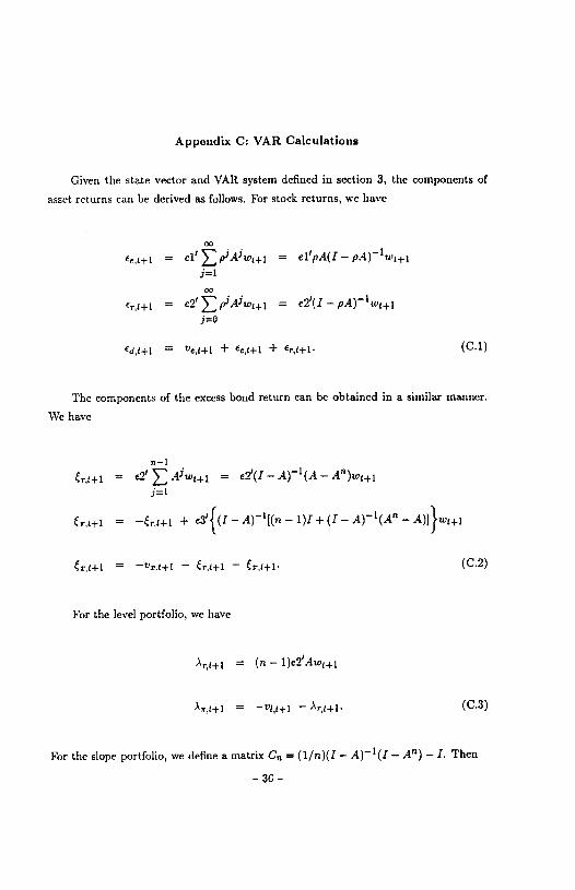
Appendix C: VAR Calculations

Given the state vector and VAR system defined in section 3, the components of

asset returns can be derived as follows. For stock returns, we have

= ef = el'pA(I —

= e2'>p.1A3w1j = e2'(I —

= Ve,j+1 + €e,i.i + Er,z+I. (C.1)

The components of the excess bond return can be obtained in a similar manner.

We have

n—i= e2' = e21(I — —

= —Et+i + e3'{(I — — 1)1 + (I — A)i(An —

= — eT,i+i — (C.2)

For the level portfolio, we have

= (n — 1)e2'Awg+i

= v1,g÷i— Ar,t+i. (C.3)

For the slope portfolio, we define a matrix C,, = (1/n)(I — — Atm) — I. Then

— 36 —

/Lrt+I = (n —

= — (n — 1)e3'(I —

/1x,t+1 = z,t+1 = Vm+1 — — (C.4)

— 37 —

Bibliography

Barsky, Robert B., 1989, "Why Don't the Prices of Stocks and Bonds Move Together?",American Economic Review 79:1132—1145.

Barsky, Robert B. and J. Bradford DeLong, 1989, "Why Have Stock Prices Fluctu-ated?", unpublished paper.

Campbell, John V., 1987, "Stock Returns and the Term Structure", Journal of Finan-cial Economics 18:373—399.

Campbell, John Y., 1990a, "Measuring the Persistence of Expected Returns", AmcricanEconomic Review Papers and Proceedings 80:43—47.

Campbell, John Y., 1990b, "Intertemporal Asset Pricing without Consumption", Fi-nancial Research Center Memorandum No. 119, Princeton University.

Campbell, John Y., 1991, "A Variance Decomposition for Stock Returns", the HG.Johnson Lecture to the Royal Economic Society, Economic Journal 101, 157—179.

Campbell, John Y. and Robert J. Shiller, 1984, "A Simple Account of the Behaviorof Long-Term Interest Rates", with Robert J. Shiller, American Economic ReviewPapers and Proceedings 74:44—48.

Campbell, John Y. and Robert J. Shiller, 1987, "Cointegration and Tests of PresentValue Models", Journal of Political Economy 95:1062—1088.

Campbell, John Y. and Robert 1. Shiller, 1988a, "The Dividend-Price Ratio and Ex-pectations of Future Dividends and Discount Factors", Review of Financial Studies1:195—228.

Campbell, John Y. and Robert J. Shiller, 1988b, "Stock Prices, Earnings, and ExpectedDividends", Journal of Finance 43:661—676.

Campbell, John Y. and Robert J. Shiller, 1991, "Yield Spreads and Interest RateMovements: A Bird's Eye View", forthcoming Review of Economic Studies.

Cecchetti, Stephen C., Pok-sang Lam, and Nelson C. Mark, 1990, "Mean Reversion inEquilibrium Asset Prices", American Economic Review 80:398—418.

Conrad, Jennifer and Cautam Haul, 1988, "Time-Variation in Expected Returns",Jonrnal of Business 61:409—425.

Cutler, David M., James M. Poterba, and Lawrence H. Summers, 1989, "What MovesStock Prices?", Journal of Portfolio Management 15:4—12.

Cutler, David M., James M. Poterba, and Lawrence H. Summers, 1990, "SpeculativeDynnmies", NBER Working Paper No. 3242.

Estrella, Arturo and Gikas A. Hardouvelis, 1991, "The Term Structure as a Predictorof Real Economic Activity", Journal of Finance 46:555—576.

Fama, Eugene F., 1975, "Short Term Interest Rates as Predictors of Inflation", Amer-ican Economic Review 65:209—282.

— 38 —

Fama, Eugene F, 1984, "The Information iii the Term Structure", Journal of FinancialEconomics 13:509—528.

Faina, Eugene F., 1990a, "Stock Returns, Expected Returns, and Real Activity", Jour-nal of Finance 45:1089-1108.

Fama, Eugene F., 1990b, "Term-Structure Forecasts of Interest Rates, Inflation, andReal Returns", Journal of Monetary Economics 25:59—76.

Fama, Eugene F. and Robert R. Bliss, 1987, "The Information in Long-Maturity For-ward Rates", American Economic Review 77:680—692.

Fama, Eugene F. and Kenneth R. French, 1988a, "Permanent and Temporary Cornpo-nents of Stock Prices", Journal of Political Economy 96:246—273.

Fama, Eugene F. and Kenneth R. French, 1988b, "Dividend Yields and Expected StockReturns", Journal of Financial Economics 22:3—25.

Fama, Eugene F. and Kenneth R. French, 1989, "Business Conditions and ExpectedReturns on Stocks and Bonds", Journal of Financial Economics 25:23—49.

Fama, Eugene F. and G. William Schwert, 1977, "Asset Returns and Inflation", Journalof Financial Economics 5:115—146.

Gibbons, Michael R., 1989, "on the Volatility of Bond Prices", Carnegie.Roc/iesterConference Series on Public Policy 31:139—176.

Gibbons, Michael R. and Krishna Ramaswamy, 19S6, "The Term Structure of InterestRates: Empirical Evidence", unpublished paper, Wharton School, University ofPennsylvania.

Hansen, Lars Peter, 1982, "Large Sample Properties of Generalized Method of MomentsEstimators", Econometrica 50:1029—1054.

Hodrick, Robert J., 1991, "Dividend Yields and Expected Stock Returns: AlternativeProcedures for Inference and Measurement", Working Paper No. 88, Departmentof Finance, Kellogg School, Northwestern University.

Kandel, Shmuel and Robert F. Stambaugh, 1988, "Modelling Expected Stock Returnsfor Short and Long Horizons", Working Paper 42-88, Rodney L. White Center forFinancial Research, Wharton School, University of Pennsylvania.

Keim, Donald B. and Robert F. Stambaugh, 1986, "Predicting Returns in the Stockand Bond Markets", Journal of Financial Economics 17:357—390.

Eleidon, Allan V., 1986, "Variance Bounds Tests and Stock Price Valuation Models",Journal of Political Economy 94:953-1001.

Lchmann, Bruce N., 1991, "Earnings, Dividend Policy, and Present Value Relations:Building Blocks of Dividend Policy Invariant Cash Flows", NI3ER Working PaperNo. 3676.

Litterman, Robert B. and Laurence Weiss, 1985, "Money, Real Interest Rates andOutput: A Reinterpretation of Postwar U.S. Data", Econometrica 53:129—156.

Lo, Andrew W. and A. Craig MacKinlay, 1988, "Stock Market Prices Do Not Follow

— 39 —

Random Walks: Evidence from a Simple Specification Test", Review of FinancialStadies 1:41—66.

McCulloch, J. Huston, 1990, "U.S. Government Term Structure Data", appendix toRobert 3. Shiller "The Term Structure of Interest Rates", in Benjamin Friedmanand Frank Hahn eds. The Handbook of Monetary Economics, Amsterdam: North-Holland.

Mishkin, Frederic 5., 1990, "What Does the Term Structure Tell Us About FutureInflation?", Journal of Monetary Economics 25:77—95.

Nelson, Charles R. and Myung 3. Kim, 1990, "Predictable Stock Returns: Reality orStatistical Illusion?", NBER Working Paper No. 3297.

Poterba, James M. and Lawrence H. Summers, 1988, "Mean Reversion in Stock Prices:Evidence and Implications", Journal of Financial Economics 22:27—59.

Richardson, Matthew, "Temporary Components of Stock Prices: A Skeptic's View",unpublished paper, Graduate School of Business, Stanford University, 1989.

Richardson, Matthew and James H. Stock, 1989, "Drawing Inferences from StatisticsBased on Multi-Year Asset Returns", Journal of Financial Economics 25, 323—348.

Roll, Richard, 1988, "R2", Journal of Finance 43:541—566.

Shuller, Robert 3., 1990, "The Term Structure of Interest Rates", in Benjamin Friedmanand Frank Hahn eds. The Handbook of Monetary Economics, Amsterdam: North-Holland.

Sbiller, Robert 3. and Andrea E. Beltratti, 1990, "Stock Prices and Bond Yields: CanTheir Comovements Be Explained in Terms of Present Value Models?", NBERWorking Paper No. 3464.

Shiller, Robert 3., John Y. Campbell, and Kermit L. Schoenholtz, 1983, "Forward Ratesand Future Policy: Interpreting the Term Structure of Interest Rates", BrookingsPapers on Economic Activity 1:173—217.

Stambaugh, Robert F., 1990, "Factors in Expected Returns", unpublished paper,Wharton School, University of Pennsylvania.

Stock, James H. and Mark IV. Watson, 1990, "Business Cycle Properties of SelectedU.S. Econonuc Time Series, 1959-1988", NBER Working Paper No. 3376.

White, Halbert, 1984, Asymptotic Theory for Econometrmcians, Academic Press: Or-lando, Florida.

— 40 —

Tab

le 1

: N

otat

ion

Port

folio

E

xces

s re

turn

In

nova

tion

to

exce

ss r

etur

n N

ews

com

pone

nts

of in

nova

tion

Nom

inal

yi

eld

Nom

inal

yi

eld

spre

ad

Stoc

k e

ye

çj,e

r,fe

n-pe

riod

bon

d X

n,t

V1

yn,i

sn,

Lev

el p

ortf

olio

'n

i vj

A

, Ar

Slop

e po

rtfo

lio

mnt

em

pr

,.ur,

px

Not

es:

All

vari

able

s are

mea

sure

d in

logs

. V

aria

bles

are m

easu

red i

n re

al te

rms

unle

ss o

ther

wis

e no

ted.

The

tim

ing

conv

entio

n is

that

var

iabl

es da

ted

t are

kno

wn

at th

e en

d of

tim

e t.

Oth

er n

otat

ion

used

in th

e te

xt i

nclu

des p

t for

the

real

sto

ck p

rice

at

the

end

of t

ime . d

for t

he re

al st

ock d

ivid

end p

aid d

urin

g tim

e i,

sr+

for

the

infl

atio

n ra

te f

rom

to

t +

1, a

nd r1

for

the

real

inte

rest

rat

e re

aliz

ed a

t tim

e +

1: rj

+ =

y1,

— r1

4j. i

n A

ppen

dix

A h

+i

is u

sed

for

the

real

ret

urn

(not

exc

ess

retu

rn)

on a

sto

ck,

whi

le in

App

endi

x B

is

use

d fo

r the

nom

inal

ret

urn

(not

exc

ess

retu

rn)

on a

n n-

peri

od b

ond

and

p, is

used

for t

he n

omin

al p

rice

of a

n n-

peri

od b

ond.

Table 2: Variances, Covariances, and Correlations of Portfolio Returns

e1 1 15.965

I 0.4811952:1—1987:2 I—0.474

rn \ 0.954

Ct

/ 15.252Xj I 0.2391952:1—1979:9 ii 0.150

\ 0.089

It m0.039 —0.018 0.0419.471 0.429 0.0538.520 41.653 —0.879

0.951 —33.133 34.084

mg

0.031 0.009 0.0063.912 0.369 0.0883.199 19.243 —0.893

0.713 —16.044 16.757

meg 13.049 —0.019 —0.055 0.047

1952 : 1 — 1972: 12 xj —0.137 3.783 0.351 0.192

l —0.731 2.488 13.276 —0.852

mj 0.594 1.295 —10.788 12.083

ej ij

ej 20.159 0.075 0.008 0.030

1973: 1 — 1987 : 2 xt 1.433 17.892 0.452 0.016

i 0.327 17.343 82.362 —0.885

rn 1.106 0.550 —65.019 65.569

Notes: cj, x, l and mj are the excess returns on stocks, 10-year zero-coupon bonds, a levelportfolio of 2-month bills, and a slope portfolio long 10-year bonds and short 2-month bills.All excess returns are measured in percentage points, monthly, relative to the return on a1-month bill. Sample variances and covariances are shown along and below the diagonalof each matrix; correlations are shown in bold face above the diagonal.

Table 3: Variance Decomposition for Excess Stock Returns

VAR lag lengthSample period

152:1-87:2

1

52:1-79:91

52:1-72:121

73:1-87:23

52:1-87:2

Return RSignificance

0.0540.001

0.0960.000

0.1260.000

0.0650.106

0.0820.015

Shares of:

Var(ed)

—2Cov(d,c,)

—2Cov(a,)

Var(e,)

2Cov(,,c)

Var(c)

0.138

(0.022)

—0.016

(0.020)

0.008

(0.178)

0.016

(0.006)

0.112

(0.061)

0.742

(0.181)

0.180(0.062)

—0.017

(0.014)

0.104

(0.189)

0.006

(0.002)

—0.012

(0.048)

0.738

(0.235)

0.237

(0.112)

—0.024

(0.027)

0.179(0.125)

0.005(0.003)

—0.012

(0.041)

0.615

(0.205)

0.141

(0.070)

—0.091

(0.078)

—0.409

(0.349)

0.044

(0.028)

0.283(0.159)

1.033(0.237)

0.095(0.021)

—0.013

(0.018)

0.050

(0.120)

0.023(0.009)

0.103

(0.064)

0.742(0.133)

R2(cd)

R2(e)

R(c)

0.130(0.202)

0.257(0.183)

0.867(0.017)

0.279

(0.285)

0.012

(0.081)

0.834

(0.039)

0.417(0.210)

0.029(0.113)

0.793(0.077)

0.085

(0.170)

0.446(0.238)

0.910(0.011)

0.136(0.168)

0.202(0,174)

0.903(0.020)

Notes: This table is based on a monthly VAIl. that includes the excess stock return, real interest rate, changein the 1-month bill rate, 10-year and 2-month yield spreads, log dividend-price ratio, and relative bill rate(the difference between tIre bill rate and a 1-year backwards moving average). 'Return 1?2 is the R2 isthe regression of the excess stock return on the VAR explanatory variables, while "Significance" is the joistsignificance of the explanatory variables in tIns regression. 'I'he VAR is used to calculate the components ofthe unexpected excess stock return v11 in equation (2.2), Vt44 = eag.. i — c,,i+i — e11. The componented.i+l can be interpreted as news about future dividends, while er.f+l is news about future real interest ratesand is news about future excess stock returns. The table reports the variances and covariances of thesecomponents, divided by the variance of so that the numbers reported add up to one. The bottom panelgives the implied 112 statistics from simple regressions of vcfI on each component. Asymptotic standarderrors are reported in parentheses below each statistic in the table.

Table 4: Variance Decomposition for Excess Bond Returns

VAR lag lengthSample period

1

52:1-87:21

52:1-79:91

52:1-72:121

73:1-87:23

52:1-87:2

Return RSignificance

0.0510.002

00250.276

0.0290.383

0.0730.062

0.0920.003

Shares of:

Var((,,)

2Cov(f,4,.)

2Cov(f,)

Var(fr)

2COv(r,)

Var(f)

1.904

(0.885)

—0.209

(0.147)

—1.532

(1.482)

0.029

(0.013)

0.051

(0.108)

0.758(0.695)

1.280

(0.402)

—0.011

(0.061)

—0.452

(0.538)

0.021

(0.007)

—0.003

(0.038)

0.165

(0.173)

0.951

(0.384)

0.086

(0.079)

—0.167

(0.444)

0.018(0.013)

0.013(0.047)

0.099(0.104)

2.288(1.492)

—0.338

(0.333)

—2.172

(2.613)

0.054(0.036)

0.066(0.253)

1.102

(1.256)

2.383(1.314)

—0.287

(0.097)

—2.108

(2.205)

0.042(0.017)

0.093(0.164)

0.878(0.959)

R2(4)

R2(&)

R2()

0.560

(0.225)

0.087

(0.090)

0.000(0.011)

0.859

(0.112)

0.009(0.032)

0.024

(0.115)

0.871

(0.109)

0.255(0.189)

0.005(0.097)

0.466(0.268)

0.125(0.120)

0.002(0.026)

0.589(0232)

0.074(0.080)

0.019(0.065)

Notes: 'I'his table is based on a monthly VAR that includes the excess stock return, real interest rate,change in the 1-month bill rate, 10-year and 2-month yield spreads, log dividend-price ratio, and relativebill rate (the difference between the bill rate and a 1-year backwards moving average). "Return R2" is theimplied It2 in a regression of the excess bond return on the VAR explanatory variables, while "Significance"is the joint significance of the explanatory variables in this regression. The VAR is used to calculate thecomponents of the unexpected bond return v,i+i in equation (2.4), v,t÷i = ',i÷i — — The

component can be interpreted as news about future inflation, while is news about future realinterest rates and C,i+1 is news about future excess bond returns. The table reports the variances andcovariances of these component-s divided by the variance of v÷i so that the numbers reported add up toone. The bottom panel of the table gives the implied 162 statistics from simple regressions of v,i+i on eachcomponent. Asymptotic standard errors are reported in parentheses below each statistic in the table.

Tiibk 5; Correlation, of Cmuponont, or Bond and Stock Itoturns

0.168 —0.012 —0.051 0.060 0.111

(0.210) (0.280) (0.188) (0.306) (0.230)

1.000 0.515 —0.405 0.884 0.103

(0.201) (0.266) (0.044) (0.344)

1952: I — 1987:2 1.000 —0.181 0.783 0.273

(0.267) (0.157) (0.422)

1.000 —0.446 —0.638

(0.226) (0.210)

1.000 0.173

(0.36 1)

Cr

0.255 —0.143 0.090 0.258 0.165

(0.180) (0.263) (0.159) (0.580) (0.291)

c 1.000 —0.088 0.065 0.780 —0,031

(0.357) (0.183) (0.179) (0.317)

1952: I — 1979:9 1.000 0.005 —0.327 0.275

(0.225) (1.240) (0.534)

1.000 —0.033 —0.492

(0.188) (0.3I9)

1.000 —0.028

(0.32 1)

CONTINUED ON NEXT PAGE

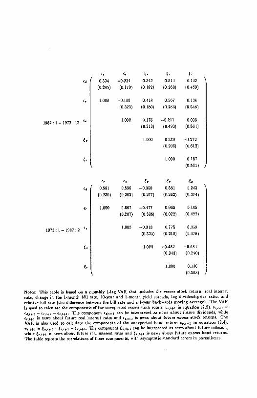
0.334 —0.234 0.342 0.514 0.142

(0.245) (0.170) (0.182) (0.260) (0.469)

1.000 —0.106 0,418 0.567 0.138

(0.323) (0.180) (0.286) (0.548)

1952: 1— 1972 121.000 0.176 —0.211 0.036

(0.213) (0.493) (0.561)

1.000 0.330 —0.272

(0.206) (0.612)

1.000 0.157

(0.561)

C, C ,.c 0.581 0.536 —0.359 0.581 0.243

(0.230) (0.282) (0.277) (0.262) (0.374)

c, 1.000 0.667 —0.477 0.965 0.165

(0.207) (0.336) (0.022) (0.492)

1973: 1 — 1987 : 2 c1.000 —0.313 0.775 0.359

(0.335) (0.210) (0.478)

1.000 —0.482 —0.684

(0.343) (0.240)

1.000 0.136

(0.508)

Notes: This table is based on a monthly 1-lag VAR that includes the excess stock return, real interestrate, change in the 1-month bill rate, 10-year and 2-month yield spreads, log dividend-price ratio, andrelative bill rate (the dilrerence between the bill rate and a 1-year backwards moving average). The VARis used to calculate the components of the unexpected excess stock return v,1.4.1 in equation (2.2), u+1Cd,i+ i — £,,l+I — e,11.i. The component d,i+ i can be interpreted as news about future dividends, whileC,i+i is news about future real interest rates and .i+i is news about future excess stock returns. TheVAR is also used to calculate the components of the unexpected bond return Vr,i.f in equation (2.4),V,i+ i = ,i+ i — r,ii-i — The component i can be interpreted as news about future inflation,while is news about future real interest rates and is news about future excess bond returns.The table reports the correlations of these components, with asymptotic standard errors in parentheses.

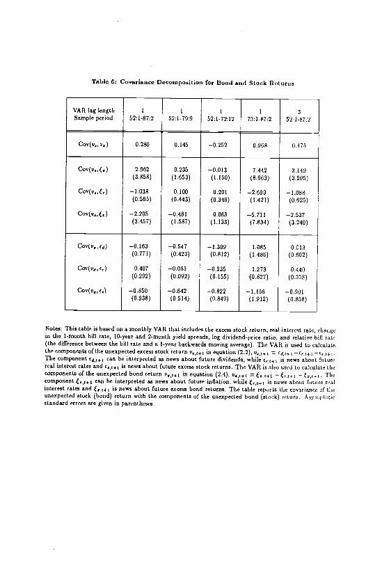
Table 6: Covariance Decomposition for I3ond and Stock Returns

VAR lag lengthSample period

1

52:1-87:21

52:1-79:91

52:1-72:121

73:1-87:23

52:1-87:2

ov(v, v) 0.280 0.145 —0.252 0.968 0.475

Cov(v,)

Cov(v.c(,)

Cov(v.,)

2.962

(3.858)

—1.038

(0.565)

—2.205

(3.457)

0.235

(1.653)

0.100

(0.443)

—0.481

(1.587)

—0.013

(1.150)

0.201

(0.346)

0.063

(1.133)

7.442

(8.663)

—2.699

(1.421)

—5.711

(7.834)

3.149

(3.505)

—1.088

(0.625)

—2.537

(3.240)

Cov(v Cd)

COv(V,Cr)

Cov(v,e)

—0.163

(0.771)

0.407

(0.292)

—0.850

(0.938)

—0.547

(0.423)

0.051

(0.092)

—0.642

(0.514)

—1.309

(0.812)

—0.235

(0.155)

—0.822

(0.849)

1.085

(1.486)

1.273

(0.827)

—1.156

(1.912)

0.013

(0.602)

0.440

(0.308)

—0.901

(0.858)

Notes: This table is based on a monthly VAR that includes the excess stock return, real interest rate, changein the 1-month bill rate, 10-year and 2-month yield spreads, log dividend-price ratio, and relative bill rate(the difference between the bill rate and a 1-year backwards moving average). The VAR is used to calculatethe components of the unexpected excess stock return v4.i in equation (2.2), v,,t+i = d,t+1 r,--tThe component can be interpreted as news about future dividends, while e1 is news about futurereal interest rates and e+j is news about future excess stock returns. The VAR is also used to calculate thecomponents of the unexpected bond return v1j in equation (2.4), v4.j = — — l'hecomponent can be interpreted as news about future inflation, while is news about future realinterest rates and is news about future excess bond returns. The table reports the covariance of tIleunexpected stock (bond) return with the components of the unexpected bond (stock) return. Asymptoticstandard errors are given in parentheses.

Table 7: Variance Deconiposition for Excess Level Portfolio Returns

VAR lag lengthSample period

1

52:1-87:2

1

52:1-79:91

52:1-72:121

73:1-87:23

52:1-87:2

Return RSignificance

0.1270.000

0.1810.000

0.2980.000

0.0960.009

0.2060.000

Shares of:

Var(As)

2Covi,A,.)

Vari,)

4.806

(1.590)

—7.638

(3.034)

3.833

(1.488)

3.128

(1.578)

—3.940

(2.740)

L812(1.240)

1.351

(1.032)

—0.974

(1.581)

0.623

(0.675)

4.825(1.445)

(2.718)

3.972(1.343)

3.318

(1.245)

—4.644

(2.264)

2.327(1.084)

R2(A,,) 0.203

(0.098)

0.000

(0.002)

0.429

(0.208)

0.014(0.062)

0.553(0.312)

0.030

(0.166)

0.178

(0.092)

0.001

(0.009)

0.299

(0.141)

0.000(0.001)

Notes: This table is based on a monthly VAR that includes the excess stock return, real interest rate, changein the 1-month bill rate, 10-year and 2-month yield spreads, log dividend-price ratio, and relative bill rate(the dillerence between the bill rate and a 1-year backwards moving average). "Return J72 is the impliedH2 in a regression of the excess return on a "level portfolio" of 2-month bills on the VAR explanatoryvariables, while "Significance" is the joint significance of the explanatory variables in this regression. The

VAR is used to calculate the components of the unexpected level portfolio return v1,÷i in equation (2.12),= A,+i — 5r,t--i- The component A,gj can be interpreted as news about future inflation, while

A,,,+i is news about future real interest rates. The table reports the variances and covariances of these

components, divided by the variance of v,1.1j so that the numbers reported add up to one. The bottom

panel of the table gives the implied K2 statistics from simple regressions of vj11 on each component.Asymptotic standard errors are reported in parentheses below each statistic in the table.

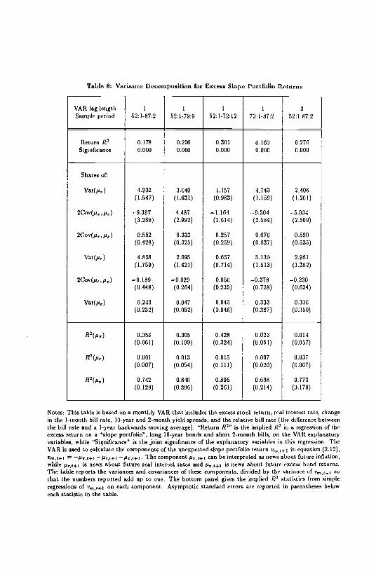
Table 8: Variance Deconapoition for Exceas Slope Portfolio Returns

VAR lag lengthSample period

1

52:1-87:21

52:1-79:91

52:1-72:121

73:1-87:23

52:1-87:2

Return 112

Significance

0.1780.000

0.2060.000

0.3010.000

0.1630.000

0.2760.000

Shares of:

Var(pe)

2COVCU5,Pr)

2Cov(p, p)

Var(p,)

2Cov(p,,pr)

Var(p5)

4.932

(1.547)

—9.397

(3.288)

0.552

(0.428)

4.858

(1.759)

0.189

(0.448)

0.243

(0.232)

3.040

(1.631)

—4.487

(2.992)

0.333

(0.325)

2.095

(1.421)

—0.029

(0.264)

0.047

(0.052)

1.157

(0.983)

—1.164

(1.614)

0.257

(0.259)

0.657

(0.714)

0.050

(0.235)

0.043

(0.046)

4.743(1.159)

—9.504

(2.584)

0.676(0.637)

5.130(1.513)

0.378

(0.728)

0.333(0.387)

2.406

(1.201)

—5.034

(2.509)

0.590

(0.535)

2.961(1.362)

0.230

(0.634)

0.306(0.350)

R2(j)

112(p)

R2(;i)

0.053(0.061)

0.001(0.007)

0.742

(0.129)

0.305(0.199)

0.013(0.054)

0.840(0.396)

0.428

(0.324)

0.015

(0.111)

0.895

(0.261)

0.023(0.051)

0.007(0.020)

0.698(0.214)

0.014

(0.057)

0.037

(0.067)

0.773

(0.170)

Notes: This table is based on a monthly VAR. that includes the excess stock return, real interest rate, changein the 1-month bill rate, 10-year and 2-month yield spreads, and the relative bill rate (the difference betweenthe bill rate and a 1-year backwards moving average). "Return R2 is the implied R. in a regression of theexcess return on a "slope portfolio", long 10-year bonds and short 2-month bills, on the VAR explanatoryvariables, while "Significance" is the joint significance of the explanatory variables in this regression. TheVAR is used to calculate the components of the unexpected slope portfolio return in equation (2.12),Vm.I = —P.1—p, The component p, can be interpreted as news about future inflation,while is news about future real interest rates and Pa.I is news about future excess bond returns.The table reports the variances and covariances of these components, divided by the variance of V,,i+I sothat, the numbers reported add up to one. The bottom panel gives the implied 112 statistics from simpleregressions of v.,.,c..i on each component. Asymptotic standard errors are reported in parentheses beloweach statistic in the table.

Table 9: Correlatioii of Components of Level and Slope Portfolio Returns

A,

A, —0.800 —0.954 0.888 —0.419

(0.039) (0.025) (0.038) (0.167)

1.000 0.958 —1.000 0.088

(0.027) (0.000) (0.184)1952 : 1 — 1987 2

1.000 —0.960 0.252

(0.025) (0.178)

1.000 —0.087

(0.183)

A, p,A, —0.827 —0.952 0.832 —0.550

(0.103) (0.030) (0.101) (0.315)

1.000 0.887 —1.000 0.040

(0.073) (0.000) (0.416)1952 : 1 — 1979 : 9

1.000 —0.889 0.440

(0.072) (0.417)

1.000 —0.047

(0.4 16)

CONTINUED ON NEXT PAGE

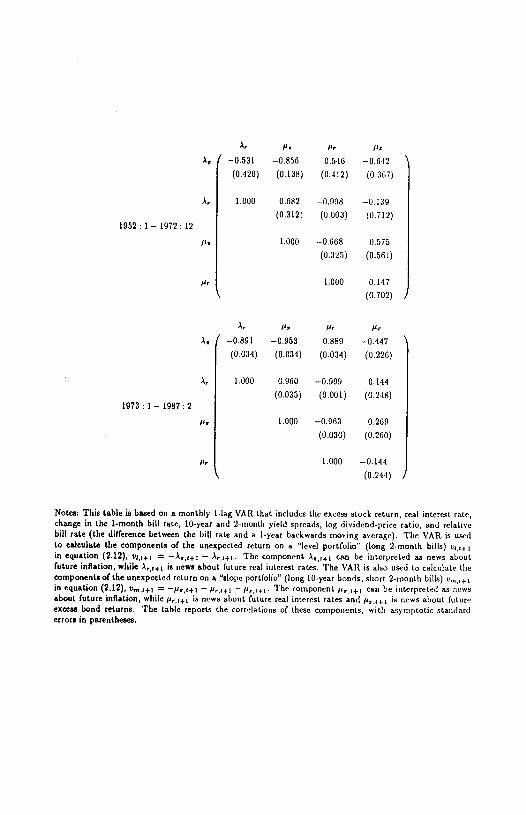
A, p. Pr P..

—0.531 —0.856 0.516 —0.642

(0.420) (0.138) (0.412) (0.367)

Ar 1.000 0.682 —0.998 0.139

(0.312) (0003) (0712)1952 1 — 1972 12

p. 1.000 —0.668 0.575

(0.325) (0.561)

Pr 1.000 0.147

(0.702) 1

A, 14. Pr 14—0.891 —0.953 0,889 —0.447

(0.034) (0.034) (0.034) (0.226)

Ar 1.000 0.960 —0.999 0.144

(0.035) (0.001) (0.218)1973 1 — 1987: 2

p. 1.000 —0.963 0.269

(0.030) (0.260)

Pr 1.000 —0.144

(0.244)

Notes: This table is based on a monthly I-lag VAR that includes the excess stock return, real interest rate,change in the 1-month bill rate, 10-year and 2-month yield spreads, log dividend-price ratio, and relativebill rate (the difference between the bill rate and a I-year backwards moving average). The VAR is usedto calculate the components of the unexpected return on a "level portfolio" (long 2-month bills) vj,.in equation (2.12), v,1+1 = —A,,+j — ,X,1+j. The component A.1+1 can be interpreted a.s news aboutfuture inflation, while is news about future real interest rates. The VAR is also used to calculate thecomponents of the unexpected return on a "slope portfolio" (long 10-year bonds, short 2-month bills) v,,,÷iin equation (212), Vm,s+l P,I+I — pr,r+i — The component /1.1+1 can be interpreted as newsabout future inflation, while Pr,i+i is news about future real interest rates and Prf I news about futureexcesa bond returns. The table reports the correlations of these components, with asymptotic standarderrors in parentheses.