JHEP07(2015)026

Published for SISSA by Springer

Received: May 1, 2015

Accepted: June 8, 2015

Published: July 7, 2015

Universal anomalous dimensions at large spin and

large twist

Apratim Kaviraj, Kallol Sen and Aninda Sinha

Centre for High Energy Physics, Indian Institute of Science,

C.V. Raman Avenue, Bangalore 560012, India

E-mail: apratim@cts.iisc.ernet.in, kallol@cts.iisc.ernet.in,

asinha@cts.iisc.ernet.in

Abstract: In this paper we consider anomalous dimensions of double trace operators at

large spin (`) and large twist (τ) in CFTs in arbitrary dimensions (d ≥ 3). Using analytic

conformal bootstrap methods, we show that the anomalous dimensions are universal in the

limit ` τ 1. In the course of the derivation, we extract an approximate closed form

expression for the conformal blocks arising in the four point function of identical scalars in

any dimension. We compare our results with two different calculations in holography and

find perfect agreement.

Keywords: Gauge-gravity correspondence, 1/N Expansion

ArXiv ePrint: 1504.00772

Open Access, c© The Authors.

Article funded by SCOAP3.doi:10.1007/JHEP07(2015)026

JHEP07(2015)026

Contents

1 Introduction 1

2 Approximate conformal blocks in general d 3

3 Anomalous dimensions for general d 5

4 Leading n dependence of γn 6

4.1 Even d 8

4.2 Odd d 9

5 CFT vs. holography 10

5.1 Comparison with the Eikonal limit calculation 10

5.2 Another gravity calculation 11

6 Discussions 16

A Exact n dependence in d = 6 17

1 Introduction

With the recent resurgence in the applications [1–14] of the conformal bootstrap program

in higher dimensions, it is of interest to ask which of these results are universal and will

hold for any conformal field theory (under some minimal set of assumptions). Among other

things, such results may prove useful tests for the burgeoning set of numerical tools (see

e.g. [15–18]) being used in the program. In this paper we will prove one such result in any

d-dimensional CFT with d ≥ 3.

We will consider CFTs in dimensions greater than two. We will assume that there is a

scalar operator of dimension ∆φ and a minimal twist (τ = d−2) stress energy tensor. Then

using the arguments of [19, 20], one finds that there is an infinite sequence of large spin

operators of twists τ = 2∆φ + 2n where n ≥ 0 is an integer. By assuming that there is a

twist gap separating these operators from other operators in the spectrum, we can go onto

setting up the bootstrap equations which will enable us to extract the anomalous dimension

γ(n, `) of these operators [19–21]. In [21], we derived γ(n, `) for 4d-CFTs satisfying the

above conditions in the large spin limit. We found that the n 1 result was universal in

the sense that it only depended on n, ` and cT the coefficient appearing in the two point

function of stress tensors, with no dependence on ∆φ. We were able to show an exact

agreement with the Eikonal limit calculation by Cornalba et al. [22–24]. In this paper we

will extend this analysis to arbitrary dimensions greater than two.

– 1 –

JHEP07(2015)026

One of the key results which will enable us to perform this calculation is the derivation

of a closed form expression for the conformal blocks in arbitrary dimensions in a certain

approximation. This was already initiated in [19, 20] and we will take this to the logical

conclusion needed to extract the anomalous dimensions. In particular, we will derive an

expression that solves a recursion relation (see eq. (70) appendix A of [19] which follows

from [25]) relating the blocks in d dimensions to the blocks in d − 2 dimensions. In the

large spin limit, the blocks simplify and approximately factorize. This is what allows us to

perform analytic calculations.

We find that the anomalous dimensions γ(n, `) in the limit ` n 1 take on the form

γ(n, `) = − 8(d+ 1)

cT (d− 1)2

Γ(d)2

Γ(d2

)4 nd

`d−2. (1.1)

Here cT is the coefficient appearing in the two point function of stress tensors. Since ` 1

we do not need cT to be large to derive this result. However, if cT is large we can identify

the operators as double trace operators. One of the main motivations for looking into this

question was an interesting observation made in [26] which relates the sign of the anomalous

dimensions1 of double trace operators with Shapiro time delay suggesting an interesting

link between unitarity of the boundary theory and causality in the bulk theory. We found

in [21], that γ(1, `) could be positive if ∆φ violated the unitarity bound.

We will show that the bootstrap result is in exact agreement with the holographic

calculation performed in [22]. In this calculation, one needs to assume both large spin and

large twist. Moreover, why the sign of the anomalous dimension is negative as well as why

the result for the anomalous dimension in this limit is independent of α′ corrections are

somewhat obscure. We will turn to another calculation in holography, proposed in [28]

which has three advantages: (a) one can consider ` 1 but n not necessarily large (b) it

makes it somewhat more transparent why α′ corrections do not contribute to the leading

order result except through cT and (c) it relates the negative sign of the anomalous dimen-

sion to the positive sign of the AdS Schwarzschild black hole mass. We will extend the

results of [28] who considered n = 0 to finite n.

Our paper is organized as follows. In section 2, we write down a closed form expression

in a certain approximation for conformal blocks [25, 29, 30] in general dimensions. In

section 3, we set up the calculation of anomalous dimensions (for double trace operators)

in general dimensions ≥ 3 using analytic bootstrap methods. In section 4, we perform

the sums needed in the limit ` n 1 and derive the universal result eq. (1.1). In

section 5, we turn to holographic calculations of the same results. We conclude with a brief

discussion of open problems in section 6. Appendix A shows the exact n dependence in

d = 6 extending the d = 4 result [21].

1See [27] for a recent work on the sign of anomalous dimensions in N = 4 Yang-Mills in perturbation

theory.

– 2 –

JHEP07(2015)026

2 Approximate conformal blocks in general d

We start with the bootstrap equation used in [19, 21],2

1 +1

4

∑`m

Pmuτm2 fτm,`m(0, v) +O

(uτm2

+1)

=

(u

v

)∆φ∑τ,`

Pτ,`g(d)τ,` (v, u) . (2.1)

For general d dimensional CFT, the minimal twist τm = d − 2. This is the twist for the

stress tensor which we will assume to be in the spectrum. The function fτm,`m(0, v) is of

the form,

fτm,`m(0, v) = (1− v)`m 2F1

(τm2

+ `m,τm2

+ `m, τm + 2`m, 1− v). (2.2)

On the r.h.s. of (2.1), g(d)τ,` (v, u) denote the conformal blocks in the crossed channel. In the

limit of the large spin, g(d)τ,` (v, u) undergo significant simplification as given in appendix A

of [19]. For any general d, the function g(d)τ,` (v, u) can be written as,

g(d)τ,` (v, u) = k2`+τ (1− u)F (d)(τ, v) +O(e−2`

√v) , (2.3)

where subleading terms are exponentially suppressed at large ` and,

kβ(x) = xβ/2 2F1

(β

2,β

2, β, x

). (2.4)

In the limit of large ` and fixed τ and for u→ 0, following appendix A of [19],

g(d)τ,` (v, u) = k2`(1− u)vτ/2F (d)(τ, v) +O

(1/√`,√u). (2.5)

Thus to the leading order we need to find the functions F (d)(τ, v) to complete the derivation

of the factorizaion ansatz given in (2.5).

To derive a form of the function F (d)(τ, v), we start by writing down the recursion rela-

tion relating the conformal block in d dimension to the ones in d−2 dimensions (see [19, 25]),(z − z

(1−z)(1−z)

)2

g(d)∆,`(v, u) =

g(d−2)∆−2,`+2(v, u)− 4(`−2)(d+`−3)

(d+2`−4)(d+2`−2)g

(d−2)∆−2,`(v, u)

− 4(d−∆−3)(d−∆−2)

(d−2∆−2)(d−2∆)

[(∆+`)2

16(∆+`−1)(∆+`+1)g

(d−2)∆,`+2(v, u)

− (d+`−4)(d+`−3)(d+`−∆−2)2

4(d+2`−4)(d+2`−2)(d+`−∆−3)(d+`−∆−1)g

(d−2)∆,` (v, u)

],

(2.6)

where u = zz and v = (1 − z)(1 − z). In the limit when ` → ∞ at fixed τ = ∆ − `,

(2.6) becomes,(z − z

(1− z)(1− z)

)2

g(d)τ,` (v, u)

`1= g

(d−2)τ−4,`+2(v, u)− g(d−2)

τ−2,` (v, u)− 1

16g

(d−2)τ−2,`+2(v, u)

+(d− τ − 2)2

16(d− τ − 3)(d− τ − 1)g

(d−2)τ,` (v, u) +O

(1

`

).

(2.7)

2The factor of 14

on the l.h.s. is to match with the conventions of [21].

– 3 –

JHEP07(2015)026

Furthermore for z → 0 and z z = 1− v +O(z) < 1 we can write the l.h.s. of (2.7) as,(z − z

(1− z)(1− z)

)2

g(d)τ,` (v, u)

u→0=

[(1− vv

)2

+O(u)

]g

(d)τ,` (v, u) . (2.8)

Finally putting in the factorization form in (2.5), we get,

(1− v)2F (d)(τ, v) = 16F (d−2)(τ − 4, v)− 2vF (d−2)(τ − 2, v)

+(d− τ − 2)2

16(d− τ − 3)(d− τ − 1)v2F (d−2)(τ, v)

+O(1/√`,√u) .

(2.9)

We find F (d)(τ, v) to be,3

F (d)(τ, v) =2τ

(1− v)d−2

2

2F1

(τ − d+ 2

2,τ − d+ 2

2, τ − d+ 2, v

). (2.10)

To see whether (2.10) satisfies the recursion relation in (2.9), we plug in (2.10) in (2.9) and

expand both sides in powers of v. Then the l.h.s. is,

(1− v)2F (d+2)(τ, v) =∞∑k=0

vk 2−2+τ

(d2 − 4k − 2d(−2 + τ) + (−2 + τ)2

)Γ2(− 1− d

2 + k + τ2

)Γ(−d+ τ)

(1− v)d−2

2 Γ2(1 + k)Γ2(−d+τ

2

)Γ(−d+ k + τ)

.

(2.11)

The r.h.s. under power series expansion gives,

16F (d)(τ − 4, v)− 2vF (d)(τ − 2, v) +(d− τ)2

16(d− τ − 1)(d− τ + 1)v2F (d)(τ, v) =

∞∑k=0

vk

(1− v)d−2

2

(2−4+τ (d− τ)2Γ2

(− 1− d

2 + k + τ2

)Γ(2− d+ τ)

(−1 + d2 − 2dτ + τ2)(−2 + k)!Γ2(

2−d+τ2

)Γ(−d+ k + τ)

+2τΓ(−2− d+ τ)Γ2

(k − 2+d−τ

2

)k!Γ2

(−2−d+τ2

)Γ(−2− d+ k + τ)

−2τ−1Γ(−d+ τ)Γ2

(− 1 + k − d−τ

2

)(−1 + k)!Γ2

(−d+τ2

)Γ(−1− d+ k + τ)

).

(2.12)

Using properties of gamma functions the above series simplifies to the one given in (2.11).4

Since the two series are the same, the expression (2.10) is the solution to the recursion

relation (2.9) for any d.5 With the knowledge of F (d)(τ, v) for general d, we can now do the

same analysis for the anomalous dimensions in general d, following what was done in [21]

for d = 4.

3We guessed this form of the solution by looking at the explicit forms of F (d)(τ, v) for d = 2, 4.4We have checked in Mathematica that the expression in (2.12) after FullSimplify matches with (2.11).5One can show that using (2.10) in (2.1) reproduces the exact leading term 1, on the l.h.s., by cancelling

all the subleading powers of v. This shows that (2.10) is indeed the correct form of F (d)(τ, v) for general d.

– 4 –

JHEP07(2015)026

3 Anomalous dimensions for general d

F (d)(τ, v) can be written as,

F (d)(τ, v) =2τ

(1− v)d−2

2

∞∑k=0

dτ,kvk, where, dτ,k =

((τ − d)/2 + 1

)k

2

(τ − d+ 2)kk!, (3.1)

where (a)b = Γ(a+b)/Γ(a). The MFT coefficients for general d, after the large ` expansion

takes the form,

P2∆φ+2n,``1≈√π

4`q∆φ,n`

2∆φ−3/2, (3.2)

where,

q∆φ,n = 23−τ Γ(∆φ + n− d/2 + 1)2Γ(2∆φ + n− d+ 1)

n!Γ(∆φ)2Γ(∆φ − d/2 + 1)2Γ(2∆φ + 2n− d+ 1). (3.3)

The r.h.s. of (2.1) can be written as,∑τ,`

PMFTτ,` v

τ2−∆φz∆φ(1− v)∆φk2`(1− z)F (d)(τ, v) . (3.4)

The twists are given by τ = 2∆φ + 2n + γ(n, `). Thus in the large spin limit, to the first

order in γ(n, `) we get,

∑n,`

PMFT2∆φ+2n,`

[γ(n, `)

2log v

]vn`

12 4`√πK0(2`

√z)z∆φ(1− v)∆φF (d)(2∆φ + 2n, v) , (3.5)

where K0(2`√z) is the modified Bessel function. Moreover for large `, the anomalous

dimensions behaves with ` like (see [19, 21]),

γ(n, `) =γn`τm

, (3.6)

where τm is the minimal twist. With this we can convert the sum over ` into an integral [19,

21] giving,

z∆φ

∫ ∞0

`2∆φ−1−τmK0(2`√z) =

1

4Γ

(∆φ −

τm2

)2

zτm2 . (3.7)

Thus the r.h.s. of (2.1) becomes,

1

16Γ

(∆φ −

τm2

)2

zτm2

∑n

q∆φ,n log v vnγn(1− v)∆φF (d)(2∆φ + 2n, v) . (3.8)

On the l.h.s. of (2.1), we will determine the coefficients of vα as follows. To start with,

we move the part (1− v)∆φ−(d−2)/2 in (3.8) on the l.h.s. to get the log v dependent part,

− Pm4

(1− v)bΓ(τm + 2`m)

Γ(τm/2 + `m)2

∞∑n=0

((τm/2 + `m)n

n!

)2

vn log v , (3.9)

– 5 –

JHEP07(2015)026

where b = τm2 + `m + d−2

2 −∆φ. Rearranging (3.9) as∑∞

α=0Bdαv

α, where n + k = α and

then summing over k from 0 to ∞ gives the coefficients Bdα,

Bdα = −4PmΓ(τm + 2`m)

Γ(τm/2 + `m)2

α∑k=0

(−1)k(

(τm/2 + `m)α−k(α− k)!

)2 b!

k!(b− k)!

= −4PmΓ(τm + 2`m)Γ(τm/2 + `m + α)2

Γ(1 + α)2Γ(τm/2 + `m)4

× 3F2

(− α,−α,−b; 1− `m −

τm2− α, 1− `m −

τm2− α; 1

).

(3.10)

The coefficient of vα log v in (3.8) thus becomes,

Hα = Γ

(∆φ −

τm2

)2 α∑k=0

22∆φ+2α−2kq∆φ,α−k d2∆φ+2α−2k,k γα−k , (3.11)

where we have put τ = 2∆φ + 2n and further n = α − k due to the fact that we have

regrouped terms in v with same exponent α and dp,k is given by (3.1). Equating Hα = Bdα

for general d dimensions,6 we get following the steps in [21],

γn =n∑

m=0

Cdn,mBdm , (3.12)

where for general d dimensions, the coefficients Cdn,m takes the form,

Cdn,m =(−1)m+n

8

Γ(∆φ)2

(∆φ − d/2 + 1)m2

n!

(n−m)!

(2∆φ + n+ 1− d)mΓ(∆φ − τm/2)2

, (3.13)

where τm = d−2 for non zero `m and the general d dimensional coefficients Bdm for general

d dimensions is given in (3.10).

4 Leading n dependence of γn

To find the full solution7 for the coefficients γn of the anomalous dimensions in general

dimensions is a bit tedious. Nonetheless we can always extract the leading n dependence

of the coefficients for large n. γn can be written as,

γn =n∑

m=0

an,m , (4.1)

where,

an,m = −Pm(−1)m+nΓ(n+ 1)Γ(2 + 2δ)Γ(∆φ)2Γ(1 + δ +m)2Γ(1 +m+ n− 2δ + 2∆φ)

2Γ(1 + δ)4Γ(1 + n− 2δ + 2∆φ)Γ(n−m+ 1)Γ(m+ 1)2Γ(1 +m− δ + ∆φ)2

×m∑k=0

(−m)k2(x)k

(−m− δ)k2 k!, (4.2)

6In [31], there was a numerical study of this recursion relation for d = 4.7We present the d = 6 solution in the appendix. The d = 4 solution can be found in [21].

– 6 –

JHEP07(2015)026

where the summand is obtained by writing out 3F2 in (3.10) explicitly, δ = d/2 and

x = ∆φ−2δ. To find the leading n dependence we need to extract the leading m dependence

inside the summation in (4.2). To do that we expand the summand around large m upto

2δ terms and then perform the sum over k from 0 to m. The large m expansion takes the

form,m∑k=0

(−m)k2(x)k

(−m− δ)k2 k!

m1≈ Γ(2δ + 1)Γ(m+ x+ 1)

Γ(m+ 1)Γ(x+ 2δ + 1)+ · · · . (4.3)

The terms in · · · are the subleading terms which will not affect8 the leading order result

in n. Thus to the leading order,

an,m ≈ −Pm(−1)m+nΓ(n+ 1)Γ(2 + 2δ)Γ(∆φ)2Γ(1 + δ +m)2Γ(1 +m+ n− 2δ + 2∆φ)

2Γ(1 + δ)4Γ(1 + n− 2δ + 2∆φ)Γ(n−m+ 1)Γ(m+ 1)2Γ(1 +m− δ + ∆φ)2

×Γ(2δ + 1)Γ(m+ ∆φ − 2δ + 1)

Γ(m+ 1)Γ(∆φ + 1). (4.4)

We can now separate the parts of an,m into,

an,m = −Pm(−1)m+nΓ(2δ + 1)Γ(2 + 2δ)Γ(∆φ)2

2Γ(1 + δ)4Γ(1 + n− 2δ + 2∆φ)Γ(∆φ + 1)×

Γ(1 +m+ n− 2δ + 2∆φ)

Γ(1 +m− δ + ∆φ)

× n!

m!(n−m)!

[Γ(m+ δ + 1)2

Γ(m+ 1)2

Γ(m+ ∆φ − 2δ + 1)

Γ(m+ ∆φ − δ + 1)

].

(4.5)

The leading term inside the bracket is mδ. Thus to the leading order in m, the coefficient

an,m is given by,

an,m = −Pm(−1)m+nΓ(2δ + 1)Γ(2 + 2δ)Γ(∆φ)2

2Γ(1 + δ)4Γ(1 + n− 2δ + 2∆φ)Γ(∆φ + 1)×

Γ(1 +m+ n− 2δ + 2∆φ)

Γ(1 +m− δ + ∆φ)

× n!mδ

m!(n−m)!,

(4.6)

for general d dimensions. Note that to reach (4.6), we just extracted the leading m de-

pendence without making any assumptions about δ apart from δ > 0 and δ ∈ R. More

specifically δ takes integer values for even dimensions and half integer values for odd di-

mensions. We will now need to analyze the m dependent part of an,m. For that note first

that using the reflection formula,

Γ(1 +m− δ + ∆φ)Γ(δ −m−∆φ) = (−1)mπ

sin(1− δ + ∆φ)π, (4.7)

we can rewrite the coefficients an,m as,

an,m = (−1)n+1 sin(∆φ − δ)ππ

Pmn!Γ(2δ + 1)Γ(2 + 2δ)Γ(∆φ)2

2Γ(1 + δ)4Γ(∆φ + 1)Γ(1 + n− 2δ + 2∆φ)

mδ

m!(n−m)!Γ(1 +m+ n− 2δ + 2∆φ)Γ(δ −m−∆φ) .

(4.8)

8This can be explicitly checked in Mathematica.

– 7 –

JHEP07(2015)026

Further using the integral representation of the product of the Γ-functions,

Γ(1 +m+ n− 2δ + 2∆φ)Γ(δ −m−∆φ) =

∫ ∞0

∫ ∞0dxdy e−(x+y)xm+n−2δ+2∆φyδ−m−∆φ−1,

(4.9)

we pull the m dependent part of an,m inside the integral and perform the summation over

m to get,

γn = (−1)n+1 sin(∆φ − δ)ππ

Pmn!Γ(2δ + 1)Γ(2 + 2δ)Γ(∆φ)2

2Γ(1 + δ)4Γ(∆φ + 1)Γ(1 + n− 2δ + 2∆φ)

×∫ ∞

0

∫ ∞0dxdy e−(x+y)xn−2δ+2∆φyδ−∆φ−1

n∑m=0

(x

y

)m mδ

m!(n−m)!.

(4.10)

At this stage we will need the explicit information about whether δ is integer or half integer.

4.1 Even d

For even dimensions, δ is an integer. The summation over m can be performed with ease

now. We first put z = log(x/y). After this substitution, the summand can be written as,

n∑m=0

(x

y

)m mδ

m!(n−m)!=

n∑m=0

mδ

m!(n−m)!emz. (4.11)

It is easy to see that starting from a function fn(z) and acting ∂z repeatedly on it can give

back the above sum provided,

fn(z) =

n∑m=0

emz

m!(n−m)!=

(1 + ez)n

n!. (4.12)

For integer δ,n∑

m=0

mδ

m!(n−m)!emz = ∂δzfn(z) . (4.13)

The leading order term in the derivatives of the generating function fn(z) is of the form

∂δzfn(z) =Γ(n+ 1)

n!Γ(n+ 1− δ)(1 + ez)n(1 + e−z)−δ + · · · , (4.14)

where · · · represent the subleading terms in n. Substituting for z and then into the integral

representation in (4.10), we get,

γn = (−1)n+1 sin(∆φ − δ)ππ

Pmn!Γ(2δ + 1)Γ(2 + 2δ)Γ(∆φ)

2Γ(1 + δ)4∆φΓ(1 + n− 2δ + 2∆φ)(n− δ)!

×∫ ∞

0

∫ ∞0dxdy e−(x+y)xn−2δ+2∆φyδ−∆φ−1

(x+ y

y

)n( x

x+ y

)δ.

(4.15)

The integral can be performed by a substitution of variables x = r2 cos2 θ and y = r2 sin2 θ

and integrating over r = 0,∞ and θ = 0, π2 . This gives,

γn = −sin(∆φ−δ)π

π

Pmn!Γ(2δ+1)Γ(2+2δ)Γ(∆φ)

2Γ(1+δ)4∆φΓ(1+n−2δ+2∆φ)(n−δ)!π csc(∆φ−δ)π

Γ(1+n−δ+2∆φ)

Γ(1+∆φ)

= −PmΓ(2δ + 1)Γ(2δ + 2)

2Γ(1 + δ)4∆2φ

Γ(n+ 1)Γ(1 + n− δ + 2∆φ)

Γ(n+ 1− δ)Γ(1 + n− 2δ + 2∆φ). (4.16)

– 8 –

JHEP07(2015)026

The leading term in n for the last ratio in (4.16) is n2δ giving the leading n dependence of

γn for even dimensions as,

γn = −PmΓ(2δ + 1)Γ(2δ + 2)

2Γ(1 + δ)4∆2φ

n2δ. (4.17)

4.2 Odd d

In odd d as well we will start with (4.10) but in this case the calculation is slightly different

from the previous one in the sense that now δ takes half integer values. We start by writing

δ = p− 1/2 where p ∈ Z, and separate the√m contribution by an integral representation,

√π√m

=

∫ ∞−∞

e−mt2dt . (4.18)

We can now write the sum in (4.10) for half integer δ as,

n∑m=0

mp emz√mm!(n−m)!

=1√π

n∑m=0

mp

m!(n−m)!

∫ ∞−∞

em(z−t2)dt . (4.19)

Here p ∈ Z. The generating function fn(z) for this case which provides with the above

expression is,

fn(z) =1√π

∫ ∞−∞

(1 + ez−t2)n

n!dt , (4.20)

and (4.19) is,n∑

m=0

mp emz√mm!(n−m)!

= ∂pzfn(z) . (4.21)

The leading order term in ∂pzfn(z) is given by,

∂pzfn(z) =1√π

Γ(n+ 1)

n!Γ(n+ 1− p)

∫ ∞−∞

dt

(1 + ez−t2)n−p(ez−t

2)p + · · ·

, (4.22)

where · · · are the subleading terms which does not affect the leading order results. We can

now determine the integral by saddle point method by letting the integrand as,

eg(t,z), where g(t, z) = (n− p) log[1 + ez−t

2]+ p(z − t2) . (4.23)

Setting g′(t, z) = 0 we see that the saddle is located at t = 0. Expanding around the saddle

point upto second order the integrand becomes,

exp[g(t, z)] = exp

[g(0, z) +

1

2g′′(0, z)t2 + · · ·

], (4.24)

where the terms in · · · contribute at O(1/n) after carrying out the integral over t. Thus

to the leading order,

∂pzf(n(z) =1√π

Γ(n+1)

n!Γ(n+1−p)

√2π

−g′′(0, z)eg(0,z) =

Γ(n+1)

n!Γ(n+1−p)1√n

(1 + ez)n(1 + e−z)−δ,

(4.25)

– 9 –

JHEP07(2015)026

where δ = p− 1/2. Substituting for z, we get the leading order in n as,

∂pzf(n(z) =nδ

n!

(x+ y

y

)n( x

x+ y

)δ. (4.26)

We can now substitute (4.26) into (4.10) and carry out the integral over x and y giving

us back,

γn = −PmΓ(2δ + 1)Γ(2δ + 2)

2Γ(1 + δ)4∆2φ

Γ(1 + n− δ + 2∆φ)

Γ(1 + n− 2δ + 2∆φ)nδ. (4.27)

The large n limit of the last ratio of the Γ-functions is again nδ giving,

γn = −PmΓ(2δ + 1)Γ(2δ + 2)

2Γ(1 + δ)4∆2φ

n2δ. (4.28)

Thus for both even and odd dimensions we get the universal result for the leading n

dependence for the coefficients γn,

γn = −PmΓ(d+ 1)Γ(d+ 2)

2Γ(1 + d/2)4∆2φ

nd. (4.29)

Using Pm =d2∆2

φ

(d−1)2cT[20],

γn = − d2Γ(d+ 1)Γ(d+ 2)

2(d− 1)2Γ(1 + d

2

)4cTnd = − 8(d+ 1)

cT (d− 1)2

Γ(d)2

Γ(d2

)4nd. (4.30)

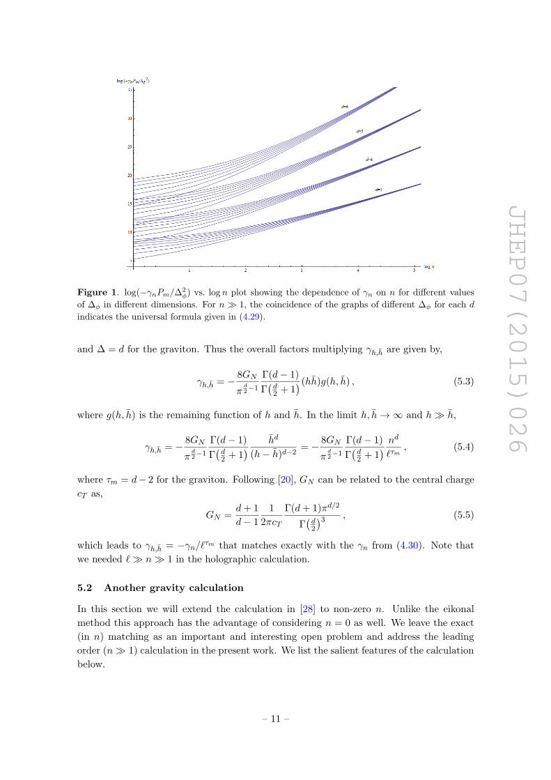
In figure 1 we show plots for γn for various dimensions for different ∆φ. At large n the

plots coincide which proves the universality of the leading order n dependence of γn.

5 CFT vs. holography

This section will focus on the matching of the findings from CFT with predictions from

holography. We start by matching the CFT coefficient Pm with the Newton constant GNappearing in the holographic calculations.

5.1 Comparison with the Eikonal limit calculation

Following [22–24] we find that in terms of the variables h = ∆φ + ` + n and h = ∆φ + n,

the anomalous dimension γh,h is,

γh,h = −16GN (hh)j−1Π⊥(h, h) , (5.1)

where Π(h, h) is the graviton (j = 2) propagator given by,

Π⊥(h, h) =1

2πd2−1

Γ(∆−1)

Γ(∆− d

2 +1)[(h−h)2

hh

]1−∆

2F1

[∆−1,

2∆−d+1

2, 2∆−d+1;− 4hh

(h−h)2

],

(5.2)

– 10 –

JHEP07(2015)026

Figure 1. log(−γnPm/∆2φ) vs. log n plot showing the dependence of γn on n for different values

of ∆φ in different dimensions. For n 1, the coincidence of the graphs of different ∆φ for each d

indicates the universal formula given in (4.29).

and ∆ = d for the graviton. Thus the overall factors multiplying γh,h are given by,

γh,h = − 8GN

πd2−1

Γ(d− 1)

Γ(d2 + 1

)(hh)g(h, h) , (5.3)

where g(h, h) is the remaining function of h and h. In the limit h, h→∞ and h h,

γh,h = − 8GN

πd2−1

Γ(d− 1)

Γ(d2 + 1

) hd

(h− h)d−2= − 8GN

πd2−1

Γ(d− 1)

Γ(d2 + 1

) nd`τm

, (5.4)

where τm = d− 2 for the graviton. Following [20], GN can be related to the central charge

cT as,

GN =d+ 1

d− 1

1

2πcT

Γ(d+ 1)πd/2

Γ(d2

)3 , (5.5)

which leads to γh,h = −γn/`τm that matches exactly with the γn from (4.30). Note that

we needed ` n 1 in the holographic calculation.

5.2 Another gravity calculation

In this section we will extend the calculation in [28] to non-zero n. Unlike the eikonal

method this approach has the advantage of considering n = 0 as well. We leave the exact

(in n) matching as an important and interesting open problem and address the leading

order (n 1) calculation in the present work. We list the salient features of the calculation

below.

– 11 –

JHEP07(2015)026

• The key idea is to write down a generic double trace operator [O1O2]n,` of quantum

number (n, `) formed from the descendants of operators O1 and O2 in the field theory,

having quantum numbers (n1, `1) and (n2, `2) where

`1 + `2 = ` , and n1 + n2 = n . (5.6)

• Such an operator is given by,

[O1O2]n,` =∑i,j

cij∂µ1 · · · ∂µ`1 (∂2)n1O1∂µ1 · · · ∂µ`2 (∂2)n2O2 , (5.7)

where cij are the Wigner coefficients that depend on n1, n2, `1 and `2. For the n = 0

case and for large `, `1 = `2 = `/2. For the n 6= 0 it is reasonable to assume that the

maxima of cij will occur, in addition to the ` variable, for n1 = n2 = n/2. Thus ∂2

will be equally distributed between the two descendents O1 and O2.

• From holography we can model the two descendants O1 and O2 as two uncharged

scalar fields with a large relative motion with respect to each other (correspond-

ing to ` 1) or equivalently one very massive object which behaves as an AdS-

Schwarzschild9 black hole and the other object moves around it with a large angular

momentum proportional to `.

• The calculation of the anomalous dimension for [O1O2]n,` from the field theory is

then equivalent to the holographic computation of the first order shift in energy of

the above system of the object rotating around the black hole.

The AdS-Schwarzschild black hole solution in d+ 1 dimensional bulk is given by,

ds2 = −U(r)dt2 +1

U(r)dr2 + r2dΩ2, (5.8)

where,

U(r) = 1− µ

rd−2+

r2

R2AdS

. (5.9)

The mass of the black hole is given by,

M =(d− 1)Ωd−1µ

16πGN. (5.10)

The first order shift in the energy is given by,10

δEdorb = 〈n, `orb|δH|n, `orb〉

= −µ2

∫rd−1drdd−1Ω〈n, `orb|

(r2−d

(1 + r2)2(∂tφ)2 + r2−d(∂rφ)2

)|n, `orb〉 .

(5.11)

9A cleaner argument may be to replace the AdS-Schwarzschild black hole with the AdS-Kerr black hole.10The normalization outside should be 1/2 and not 1/4 as used in [28]. We thank Jared Kaplan for

confirming this.

– 12 –

JHEP07(2015)026

The label ‘orb’ implies that currently we are considering one of the masses of the binary

system. We can also add higher derivative corrections coming from the α′ corrections to

the metric. This is one of the advantages of doing the anomalous dimension calculation

in this approach. It will make transparent the fact that the α′ corrections will not affect

the leading result. The metric will be modified11 by adding corrections to the factor

r2−d(1 + chα′hr−2h) where h is the order of correction in α′. The wavefunction of the

descendant state derived from the primary is given by,

ψn,`J(t, ρ,Ω) =1

N∆φn`e−iEn,`tY`,J(Ω)

[sin` ρ cos∆φ ρ 2F1

(− n,∆φ + `+ n, `+

d

2, sin2 ρ

)],

(5.12)

where En,` = ∆φ + 2n+ ` and,

N∆φn` = (−1)n

√n!Γ2(`+ d

2)Γ(∆φ + n− d−22 )

Γ(n+ `+ d2)Γ(∆φ + n+ `)

. (5.13)

Using the transformation tan ρ = r we can write the scalar operator as,

ψn,`orbJ(t, r,Ω) =1

N∆φn`orb

e−iEn,`orbtY`orb,J(Ω)

[r`orb

(1+r2)∆φ+`orb

2

n∑k=0

(−n)k(∆φ+`orb+n)k(`orb + d

2

)kk!

(r2

1+r2

)k]

=

n∑k=0

ψorbk (t, r,Ω) , (5.14)

where,

ψorbk (t, r,Ω) =

1

N∆φn`orb

e−iEn,`orbtY`orb,J(Ω)

[r`orb

(1+r2)∆φ+`orb

2

(−n)k(∆φ+`orb+n)k(`orb+ d

2

)kk!

(r2

1+r2

)k].

(5.15)

Putting (5.15) in (5.11) and carrying out the other integrals we are left with just the radial

part of the integral,

δEdorb = −µ∫r(1 + chα

′hr−2h)dr

[ n∑k,α=0

(E2n,`orb

(1+r2)2ψorbk (r)ψorb

α (r) + ∂rψorbk (r)∂rψ

orbα (r)

)]= I1 + I2 , (5.16)

where I1 and I2 are the contributions from the first and the second parts of the above

integral. The leading `orb dependence comes from the first part of the integral which is

also true for n 6= 0 case and for any general d dimensions is given by (1/`orb)(d−2)/2. Thus

we can just concentrate on the first part of the integral for the leading spin dominance of

the energy shifts. Thus the integral I1 can be written as,

I1 = − µ

N2∆φn`orb

n∑k,α=0

(−n)k(−n)α(∆φ + n+ `orb)k(∆φ + n+ `orb)α(`orb + d

2

)k

(`orb + d

2

)αk!α!

×∫ ∞

0r(1 + chα

′hr−2h)drr2`orb+2k+2α

(1 + r2)2+∆φ+`orb+k+α.

(5.17)

11There will also be an overall α′ dependent factor which can be absorbed into cT [32].

– 13 –

JHEP07(2015)026

The r integral gives,∫ ∞0r(1 + chα

′hr−2h)drr2`orb+2k+2α

(1 + r2)2+∆φ+`orb+k+α=

Γ(1 + ∆φ)Γ(1 + `orb + k + α) + chα′hΓ(1 + h+ ∆φ)Γ(1 + `orb + k + α− h)

2Γ(2 + ∆φ + `orb + k + α).

(5.18)

Hence the integral I1 becomes,

I1 = − µ

2N2∆φn`orb

n∑k,α=0

(−n)k(−n)α(∆φ + n+ `orb)k(∆φ + n+ `orb)α(`orb + d

2

)k

(`orb + d

2

)αk!α!

×Γ(1 + `orb + k + α)Γ(1 + ∆φ) + chα

′hΓ(1 + h+ ∆φ)Γ(1 + `orb + k + α− h)

Γ(2 + ∆φ + `orb + k + α).

(5.19)

Using the reflection formula for the Γ-functions we can write,

(−n)k(−n)α = (−1)k+α Γ(n+ 1)2

Γ(n+ 1− k)Γ(n+ 1− α). (5.20)

Putting in the normalization and performing the first sum over α we get,

I1 = −µ(`orb+2n)2Γ

(`orb+ d

2 +n)

2Γ(`orb+ d

2

)Γ(1− d

2 +n+∆φ

) n∑k=0

(−1)kΓ(k + `orb + n+ ∆φ)

Γ(`orb+ d

2 +k)Γ(n+1−k)Γ(2+k+`orb+∆φ)Γ(k+1)

×[Γ(1+`orb+k)Γ(1+∆φ) 3F2

(−n, k+`orb+1, `orb+n+∆φ; `orb+

d

2, 2+k+`orb+∆φ; 1

)+ chα

′hΓ(1 + `orb + k − h)Γ(1 + ∆φ + h)

× 3F2

(− n, k + `orb + 1− h, `orb + n+ ∆φ; `orb +

d

2, 2 + k + `orb + ∆φ; 1

)]. (5.21)

To the leading order in `orb (after the exapnsion in large `orb) this is the expression for δEdorb

or equivalently γn,`orbfrom the CFT for general d dimensions. Since the `orb dependence

does not rely on n dependence we can use the n = 0 to show the `orb dependence from the

α′ corrections. Thus in (5.21) we put n = 0 to get,

I1 = − µ

2Γ(1− d

2 + ∆φ

)( 1

`orb

)d−22[1 + chα

′h(

1

`orb

)h]. (5.22)

In IIB string theory α′ corrections to the metric start h = 3 due to the well known R4

term. Thus the α′ corrections contribute at a much higher order, O(1/`3orb), in 1/`orb and

hence does not affect the leading order result. In the rest of the work, we will consider only

the leading order result in `orb (set ch = 0) for general d.

For even d we can calculate I1 for n = 0, 1, 2 · · · and infer a general n dependent

polynomial. Using this polynomial, the leading n dependence of the energy shifts become,

δEdorb = −µ(

1

`orb

)d−22(

Γ(d)

Γ(d2

)Γ(d2 + 1

)nd/2 + · · ·), (5.23)

– 14 –

JHEP07(2015)026

(a) d = 3 (b) d = 5 (c) d = 7

Figure 2. The blue lines are log(`d/2−1orb δEdorb/µ) vs. log n for large values of `orb and the red lines

are the log-log plot for rhs of (5.23), in odd d. The matching of both lines at large n is the numerical

proof of (5.23) in odd d.

where · · · are terms subleading in n. For odd d the polynomial realization is less obvious

due to factors of Γ(∆φ+ 1

2

)etc. nevertheless one can show (see figure 2) at least numerically

that the leading order n dependence for odd d should also be the same as (5.23). Hence

the above form in (5.23) is true for general d dimensions.

Note that we are retrieving only half of the n dependence from (5.23). The other half

will come from the definitions of `orb, its relation with ` and µ which is related to the black

hole mass via (5.10). The relation between `orb and ` can be derived following [28]. For

the orbit state of an object rotating around a static object, `orb is related to the geodesic

length κ that maximizes the norm of the wave function (5.12). We can approximate the

hypergeometric function appearing in (5.12) by taking the large ` approximation in each

term of the sum in (5.14),

2F1

(− n,∆φ + `orb + n, `orb +

d

2, sin2 ρ

)]=

n∑k=0

(−n)k(∆φ + `orb + n)k(`orb + d

2

)kk!

(sin2 ρ)k

`orb→∞≈n∑k=0

(−n)k`korb

`korbk!sin2k ρ

= cos2n ρ . (5.24)

Using this approximation in (5.12) we find the maxima of ψ2n,`orbJ

, which occurs at,

ρ = tan−1

√`orb

2n+ ∆φ. (5.25)

Now using the relation, sinh κ = tan ρ, we find for large `orb,12

κ =1

2log

(4`orb

∆φ + n

)(5.26)

12Here there is a factor of 2 mismatch with the corresponding result given in [28]. We thank Jared Kaplan

for pointing out that this was a typo in [28].

– 15 –

JHEP07(2015)026

But our case is that of a double trace primary operator where none of the two objects is

static. However in the semi-classical limit the energy shift of the former case is same as

that of the primary if the geodesic distance between the two objects is same in both cases.

This gives, κ = κ1 + κ2, where

κ1(= κ2) =1

2log

4`1∆φ + n

. (5.27)

Since we have a composite operator which is like two particles rotating around each other,

the conformal dimension of each descendant state gets the maximum contribution when

`1 ≈ `2 ≈ `/2 and n1 ≈ n2 ≈ n/2 for large ` and n. This is why we have `/(∆φ + n) inside

log in the above equation. From (5.26) and (5.27) we get, `orb ≈ `2/n for large n. So, the

other factor sitting in front of (5.23) is given by,

µ

`orb(d−2)/2

=2GNMπ(d−2)/2Γ

(d2

)d− 1

nd/2

`d−2. (5.28)

Here we have used the equation for black hole mass (5.10). Since M relates to the case of

one massive static object at the centre, we will put M = ∆φ +n ≈ n. Using equation (5.5)

we get the anomalous dimension to be,

γ(n, `) = − 8(d+ 1)

cT (d− 1)2

Γ(d)2

Γ(d2

)4 nd

`d−2, (5.29)

which is the same as that found from CFT.

6 Discussions

We conclude by listing some open questions and interesting future problems:

• One obvious extension of our analysis is to find the full n dependent expression for

arbitrary dimensions. We know that closed form expressions exist for even dimensions

(see the appendix for the d = 6 result) but it will be interesting to see the analogous

expressions for odd dimensions. It should also be possible to repeat our analysis for

general twists τm. We restricted our attention to the case where this was the stress

tensor.

• The n ` case for arbitrary dimensions which we expect to work out in a similar

manner following [21]. In this case we needed `/n bigger than some quantity which

on the holographic side was identified with a gap — this was similar to the discussion

in [26]. This means that for operators with `/n smaller than the gap, the result would

be sensitive to α′ corrections. It could be possible that the anomalous dimensions

of these operators would not be negative indicating a problem with causality in the

bulk. It will be interesting to extend our holographic calculations to n ` 1.

• One should compare our results with those from the numerical bootstrap methods

e.g. in [15–18].

– 16 –

JHEP07(2015)026

• One could try to see if there exists a simple argument for the leading n dependence

following the lines of [33].

• It will be interesting to match the CFT and holographic calculations to all orders in

n at least for a class of theories (e.g. N = 4 results in [34]).

Acknowledgments

We thank Fernando Alday, Jared Kaplan, Shiraz Minwalla and Hugh Osborn for discussions

and correspondence. We thank Fernando Alday and Jared Kaplan for useful comments on

the draft. AS thanks Swansea University and Cambridge University for hospitality during

the course of this work. AS acknowledges support from a Ramanujan fellowship, Govt. of

India.

A Exact n dependence in d = 6

Here we will use the general d expressions discussed in section 3. For general d, γn is

given by,

γn =

n∑m=0

(4Pm)(−1)m+nnΓ(2 + d)Γ2(1 + d

2 +m)Γ2(∆φ)(1− n)m−1(d−m− n− 2∆φ)m

8Γ2(∆φ − d−2

2

)Γ4(1 + d

2

)Γ2(1 +m)

(1− d

2 + ∆φ

)m

× 3F2

[(−m,−m,−d+ ∆φ

−d2 −m,−

d2 −m

), 1

]. (A.1)

In d = 6 the hypergeometric function can be written as,

3F2

[(−m,−m,−d+ ∆φ

−d2 −m,−

d2 −m

), 1

]

=m∑k=0

(1− k +m)2(2− k +m)2(3− k +m)2Γ(−6 + k + ∆φ)

(1 +m)2(2 +m)2(3 +m)2k!Γ(−6 + ∆φ)

=36Γ(−2 +m+ ∆φ)(−2 + 2m+ ∆φ)

(10(−2 +m)m+ ∆φ(−1 + 10m+ ∆φ)

)(1 +m)(2 +m)(3 +m)Γ(4 +m)Γ(1 + ∆φ)

.

(A.2)

To see how to get the above result, we will use the tricks introduced in the appendix of [21].

Note that we can write,

(1−k+m)2(2−k+m)2(3−k+m)2 =Ak(k−1)(k−2)(k−3)(k−4)(k−5)

+Bk(k−1)(k−2)(k−3)(k−4)+Ck(k−1)(k−2)(k−3)

+Dk(k−1)(k−2)+Ek(k−1)+Fk+G , (A.3)

– 17 –

JHEP07(2015)026

where,

A = 1 ,

B = 3− 6m,

C = 3 + 15m2,

D = −2(1 + 2m)(3 + 5m(1 +m)

),

E = 3(1 +m)2(6 + 5m(2 +m)

),

F = −3(1 +m)2(2 +m)2(3 + 2m) ,

G = (1 +m)2(2 +m)2(3 +m)2.

(A.4)

So the summation in (A.2) breaks up into seven different sums of the general form shown

below,m∑k=0

k(k − 1) · · · (k − i+ 1)Γ(x+ k)

k!Γ(x)=

Γ(m+ x+ 1)

(x+ i)Γ(m− i+ 1)Γ(x). (A.5)

Once again the above result was derived in [21]. With this and summing up the respective

terms, the hypergeometric funtion simplifies to the form shown in the second line of (A.2).

The main equation (A.1) in d = 6 has the form,

γn =

n∑m=0

70(−1)n+1Pmn! Γ(−5 +m+ n+ 2∆φ)Γ(3−m−∆φ)Γ(∆φ) sin(∆φπ)

∆φm!(n−m)!Γ(−5 + n+ 2∆φ)π

× (−2 + 2m+ ∆φ)(10m2 + 10m(−2 + ∆φ) + (−1 + ∆φ)∆φ

). (A.6)

To get the above, we have used the reflection formula of gamma functions, Γ(1− z)Γ(z) =

π/ sin(πz). To do the sum we write the gamma functions in the numerator as,

Γ(3−m−∆φ)Γ(−5+m+n+2∆φ) =

∫ ∞0

∫ ∞0dxdy e−(x+y)x−6+m+n+2∆φy2−m−∆φ . (A.7)

Let us write f(m) = (−2 + 2m+ ∆φ)(10m2 + 10m(−2 + ∆φ) + (−1 + ∆φ)∆φ

). Then the

sum over m becomes,n∑

m=0

(x/y)mf(m)

m!(n−m)!=

(x+ y)n

yn(x+ y)3n!

(20n3x3 + (x+ y)3(−2 + ∆φ)(−1 + ∆φ)∆φ

+ 30n2x2(x(−2 + ∆φ) + y∆φ

)+ 2nx

(20x2 − 3(x+ y)(7x+ 2y)∆φ+ 6(x+ y)2∆φ2

)).

(A.8)

The final result can now be obtained by integrating over x and y. To do this, we change

the variables to x = r2 cos2 θ and y = r2 sin2 θ. Then we get,

γn = − 70(−1)nPmn! Γ(∆φ) sin(∆φπ)

∆φm!(n−m)!Γ(−5+n+2∆φ)π

∫ ∞0

∫ ∞0

dxdy e−(x+y)x−6+n+2∆φy2−∆φn∑

m=0

(x/y)mf(m)

m!(n−m)!

= − 70

∆2φ

Pm(20n6 + 60(−5 + 2∆φ)n5 + 10(170− 132∆φ + 27∆2

φ)n4

+ 20(−5+2∆φ)(45−32∆φ+7∆2φ)n3+2(2740−3780∆φ+2121∆2

φ−582∆3φ+66∆4

φ)n2

+ 4(−5+2∆φ)(120−140∆φ+73∆2φ−21∆3

φ+3∆4φ)n+ (−2+∆φ)2(−1+∆φ)2∆2

φ

).

(A.9)

– 18 –

JHEP07(2015)026

Figure 3. γn=1(∆2φ/Pm) vs. ∆φ plot in d = 4 (red curve) and d = 6 (blue curve), showing

that the anomalous dimension may take positive values if unitarity is violated. Unitarity demands

∆φ ≥ (d− 2)/2.

This is the result for γn in d = 6. Note that we simply extended the tricks used for

d = 4 in the appendix of [21]. The same can be done to evaluate γn for any even d > 2.

The figure 3 shows the range of ∆φ, in d = 4 and 6 for which γn=1 takes positive

values. Interestingly, for both the cases positive values of γ1 are over those values of ∆φ

which violate the respective unitarity bounds. In fact this behaviour of the anomalous

dimensions is true in any dimension. We found that for n ≥ d− 1, γn was negative for any

∆φ > 0.

Open Access. This article is distributed under the terms of the Creative Commons

Attribution License (CC-BY 4.0), which permits any use, distribution and reproduction in

any medium, provided the original author(s) and source are credited.

References

[1] R. Rattazzi, V.S. Rychkov, E. Tonni and A. Vichi, Bounding scalar operator dimensions in

4D CFT, JHEP 12 (2008) 031 [arXiv:0807.0004] [INSPIRE].

[2] R. Rattazzi, S. Rychkov and A. Vichi, Central charge bounds in 4D conformal field theory,

Phys. Rev. D 83 (2011) 046011 [arXiv:1009.2725] [INSPIRE].

[3] R. Rattazzi, S. Rychkov and A. Vichi, Bounds in 4D conformal field theories with global

symmetry, J. Phys. A 44 (2011) 035402 [arXiv:1009.5985] [INSPIRE].

[4] D. Pappadopulo, S. Rychkov, J. Espin and R. Rattazzi, OPE convergence in conformal field

theory, Phys. Rev. D 86 (2012) 105043 [arXiv:1208.6449] [INSPIRE].

[5] D. Poland, D. Simmons-Duffin and A. Vichi, Carving out the space of 4D CFTs,

JHEP 05 (2012) 110 [arXiv:1109.5176] [INSPIRE].

[6] Y. Nakayama and T. Ohtsuki, Five dimensional O(N)-symmetric CFTs from conformal

bootstrap, Phys. Lett. B 734 (2014) 193 [arXiv:1404.5201] [INSPIRE].

– 19 –

JHEP07(2015)026

[7] I. Heemskerk, J. Penedones, J. Polchinski and J. Sully, Holography from conformal field

theory, JHEP 10 (2009) 079 [arXiv:0907.0151] [INSPIRE].

[8] M. Hogervorst, H. Osborn and S. Rychkov, Diagonal limit for conformal blocks in d

dimensions, JHEP 08 (2013) 014 [arXiv:1305.1321] [INSPIRE].

[9] M. Hogervorst and S. Rychkov, Radial coordinates for conformal blocks,

Phys. Rev. D 87 (2013) 106004 [arXiv:1303.1111] [INSPIRE].

[10] C. Beem, L. Rastelli and B.C. van Rees, The N = 4 superconformal bootstrap,

Phys. Rev. Lett. 111 (2013) 071601 [arXiv:1304.1803] [INSPIRE].

[11] C. Beem, M. Lemos, P. Liendo, L. Rastelli and B.C. van Rees, The N = 2 superconformal

bootstrap, arXiv:1412.7541 [INSPIRE].

[12] F.A. Dolan, M. Nirschl and H. Osborn, Conjectures for large-N superconformal N = 4 chiral

primary four point functions, Nucl. Phys. B 749 (2006) 109 [hep-th/0601148] [INSPIRE].

[13] F.A. Dolan and H. Osborn, Superconformal symmetry, correlation functions and the operator

product expansion, Nucl. Phys. B 629 (2002) 3 [hep-th/0112251] [INSPIRE].

[14] F.A. Dolan and H. Osborn, Implications of N = 1 superconformal symmetry for chiral fields,

Nucl. Phys. B 593 (2001) 599 [hep-th/0006098] [INSPIRE].

[15] S. El-Showk et al., Solving the 3D Ising model with the conformal bootstrap,

Phys. Rev. D 86 (2012) 025022 [arXiv:1203.6064] [INSPIRE].

[16] S. El-Showk et al., Solving the 3d Ising model with the conformal bootstrap II. c-Minimization

and precise critical exponents, J. Stat. Phys. 157 (2014) 869 [arXiv:1403.4545] [INSPIRE].

[17] F. Kos, D. Poland and D. Simmons-Duffin, Bootstrapping mixed correlators in the 3D Ising

model, JHEP 11 (2014) 109 [arXiv:1406.4858] [INSPIRE].

[18] F. Gliozzi and A. Rago, Critical exponents of the 3d Ising and related models from conformal

bootstrap, JHEP 10 (2014) 042 [arXiv:1403.6003] [INSPIRE].

[19] A.L. Fitzpatrick, J. Kaplan, D. Poland and D. Simmons-Duffin, The analytic bootstrap and

AdS superhorizon locality, JHEP 12 (2013) 004 [arXiv:1212.3616] [INSPIRE].

[20] Z. Komargodski and A. Zhiboedov, Convexity and liberation at large spin,

JHEP 11 (2013) 140 [arXiv:1212.4103] [INSPIRE].

[21] A. Kaviraj, K. Sen and A. Sinha, Analytic bootstrap at large spin, arXiv:1502.01437

[INSPIRE].

[22] L. Cornalba, M.S. Costa and J. Penedones, Eikonal approximation in AdS/CFT: resumming

the gravitational loop expansion, JHEP 09 (2007) 037 [arXiv:0707.0120] [INSPIRE].

[23] L. Cornalba, M.S. Costa, J. Penedones and R. Schiappa, Eikonal approximation in

AdS/CFT: conformal partial waves and finite N four-point functions,

Nucl. Phys. B 767 (2007) 327 [hep-th/0611123] [INSPIRE].

[24] L. Cornalba, M.S. Costa, J. Penedones and R. Schiappa, Eikonal approximation in

AdS/CFT: from shock waves to four-point functions, JHEP 08 (2007) 019 [hep-th/0611122]

[INSPIRE].

[25] F.A. Dolan and H. Osborn, Conformal partial waves and the operator product expansion,

Nucl. Phys. B 678 (2004) 491 [hep-th/0309180] [INSPIRE].

– 20 –

JHEP07(2015)026

[26] X.O. Camanho, J.D. Edelstein, J. Maldacena and A. Zhiboedov, Causality constraints on

corrections to the graviton three-point coupling, arXiv:1407.5597 [INSPIRE].

[27] Y. Kimura and R. Suzuki, Negative anomalous dimensions in N = 4 SYM,

arXiv:1503.06210 [INSPIRE].

[28] A.L. Fitzpatrick, J. Kaplan and M.T. Walters, Universality of long-distance AdS physics

from the CFT bootstrap, JHEP 08 (2014) 145 [arXiv:1403.6829] [INSPIRE].

[29] F.A. Dolan and H. Osborn, Conformal four point functions and the operator product

expansion, Nucl. Phys. B 599 (2001) 459 [hep-th/0011040] [INSPIRE].

[30] F.A. Dolan and H. Osborn, Conformal partial waves: further mathematical results,

DAMTP-11-64, CCTP-2011-32 [arXiv:1108.6194] [INSPIRE].

[31] G. Vos, Generalized additivity in unitary conformal field theories, arXiv:1411.7941

[INSPIRE].

[32] K. Sen and A. Sinha, Holographic stress tensor at finite coupling, JHEP 07 (2014) 098

[arXiv:1405.7862] [INSPIRE].

[33] L.F. Alday and J.M. Maldacena, Comments on operators with large spin,

JHEP 11 (2007) 019 [arXiv:0708.0672] [INSPIRE].

[34] L.F. Alday, A. Bissi and T. Lukowski, Lessons from crossing symmetry at large-N ,

JHEP 06 (2015) 074 [arXiv:1410.4717] [INSPIRE].

– 21 –