jeffreys prior analysis of the simultaneous

JEFFREYS PRIOR ANALYSIS OF THE SIMULTANEOUS EQUATIONS MODEL IN THE CASE WITH n + 1

ENDOGENOUS VARIABLES

BY

JOHN C. CHAO and PETER C. B. PHILLIPS

COWLES FOUNDATION PAPER NO. 1107

COWLES FOUNDATION FOR RESEARCH IN ECONOMICS YALE UNIVERSITY

Box 208281 New Haven, Connecticut 06520-8281

2005

http://cowles.econ.yale.edu/

Journal of Econometrics 111 (2002) 251–283www.elsevier.com/locate/econbase

Je�reys prior analysis of the simultaneousequations model in the case with n+ 1

endogenous variablesJohn C. Chaoa ;∗, Peter C.B. Phillipsb;c;d

aDepartment of Economics, University of Maryland, College Park, MD 20742, USAbYale University, USA

cUniversity of Auckland, New ZealanddUniversity of York, UK

Abstract

This paper analyzes the behavior of posterior distributions under the Je�reys prior in a simul-taneous equations model. The case under study is that of a general limited information setupwith n + 1 endogenous variables. The Je�reys prior is shown to give rise to a marginal pos-terior density which has Cauchy-like tails similar to that exhibited by the exact �nite sampledistribution of the corresponding LIML estimator. A stronger correspondence is established inthe special case of a just-identi�ed orthonormal canonical model, where the posterior densityunder the Je�reys prior is shown to have the same functional form as the density of the �nitesample distribution of the LIML estimator. The work here generalizes that of Chao and Phillips(J. Econ. 87 (1998), 49) which gave analogous results for the special case of an equation withtwo endogenous variables.c© 2002 Elsevier Science B.V. All rights reserved.

JEL classi�cation: C11; C31

Keywords: Con�uent hypergeometric function; Je�reys prior; Laplace approximation; Posterior distribution;Simultaneous equations model; Zonal polynomials

1. Introduction

For practical applications of Bayesian statistical methods, one would often like tohave a reference prior—i.e., a roughly noninformative prior distribution against whoseresults inference that is based on more subjective priors can be compared. Since its

∗ Corresponding author. Tel.: +1-301-405-1579; fax: +1-301-405-3542.E-mail address: [email protected] (J.C. Chao).

0304-4076/02/$ - see front matter c© 2002 Elsevier Science B.V. All rights reserved.PII: S0304 -4076(02)00106 -9

252 J.C. Chao, P.C.B. Phillips / Journal of Econometrics 111 (2002) 251–283

introduction by Je�reys (1946), the Je�reys prior has been one of the most intensivelystudied reference priors in Bayesian statistics and econometrics. In particular, muchresearch has been done on the relationship between Bayesian posterior distributionsunder the Je�reys prior and frequentist sampling distributions and con�dence intervals.One prominent line of research, which goes back to the classic papers of Welch andPeers (1963) and Peers (1965) and which also includes such recent contributions asTibshirani (1989) and Nicolaou (1993), has produced an impressive body of resultsshowing, for general likelihood functions, the large sample correspondence betweenfrequentist con�dence intervals and posterior intervals based on the Je�reys prior andits variants.Similarities between frequentist results and Bayesian results derived under the Je�reys

prior have also been documented for speci�c parametric models. For the classicallinear regression model with Gaussian disturbances, the Je�reys-prior marginal posteriordistribution of each coe�cient parameter is known to be a univariate t-distribution, asis, of course, the distribution of the classical t-statistic, albeit with a slight di�erencein the degrees of freedom (cf. Zellner, 1971). On the other hand, a Je�reys-priorBayesian analysis of the linear regression model with unobserved independent variableswas �rst conducted by Zellner (1970), where it was shown that the mode of theconditional posterior density of the regression coe�cient given a ratio of the scaleparameters corresponds exactly to the maximum likelihood estimator of the coe�cientparameter. With respect to linear time series models, Phillips (1991) derives bothexact and asymptotically approximate expressions for the posterior distributions of theautoregressive parameter and �nds that on the issue of whether macroeconomic timeseries have stochastic trends, Bayesian inference based on the Je�reys prior is in muchcloser agreement with classical inference than inference based on the uniform prior.Finally, for single-equation analysis of the simultaneous equations model (SEM), Chaoand Phillips (1998) show for the special case of a just-identi�ed, orthonormal canonicalmodel with one endogenous regressor that, under the Je�reys prior, the posterior densityof the coe�cient of the endogenous regressor has the same Cauchy-tailed, in�niteseries representation as the exact sampling distribution of the LIML estimator givenby Mariano and McDonald (1979). Moreover, even when this model is overidenti�edof order one, Chao and Phillips (1998) show that, analogous to the �nite sampledistribution of the LIML estimator, the posterior density of the structural coe�cientunder the Je�reys prior has no moment of positive integer order.Because of its prominence as a reference prior, as evident from the literature cited

above, it seems important to develop a good understanding of how the use of theJe�reys prior a�ects statistical inference in situations of interest to econometricians.Our main purpose in this paper is to contribute to this understanding within thecontext of the simultaneous equations model. Our work builds on Chao and Phillips(1998) and generalizes results obtained in that paper to the case with n endogenousregressors. In particular, analogous to the single endogenous regressor case, we showthat a Je�reys-prior, single-equation analysis of a just-identi�ed, orthonormal canoni-cal model with n endogenous regressors leads to a posterior density for the structuralcoe�cient vector � which has the same in�nite series representation in terms of zonalpolynomials as the �nite sample density of the LIML estimator, derived by Phillips

J.C. Chao, P.C.B. Phillips / Journal of Econometrics 111 (2002) 251–283 253

(1980). In addition, even if we allow for an arbitrary degree of overidenti�cation andan arbitrary, non-canonical reduced-form error covariance structure, the posterior den-sity of � under the Je�reys prior still exhibits the same tail behavior as the smallsample distribution of LIML.The paper is organized as follows. Section 2 discusses the various model and prior

speci�cations to be studied in the paper. Section 3 presents exact posterior resultsfor the orthonormal, canonical model (to be de�ned below). Section 4 gives a the-orem which characterizes the tail behavior of the Je�reys-prior posterior density of� in the general case and provides some numerical evaluation of the accuracy ofthe Laplace approximation derived in Chao and Phillips (1998). We o�er some con-cluding remarks in Section 5 and leave all proofs and technical material for theappendix.Before proceeding, we brie�y introduce some notations. In what follows, we use

tr(·) to denote the trace of a matrix, |A| = |det(A)| to denote the absolute value ofthe determinant of A, and r(�) to signify the rank of the matrix �. The inequality“¿ 0” denotes positive de�nite when applied to matrices; vec(·) stacks the rows ofa matrix into a column vector; the symbol “≡” denotes equivalence in distributionand the symbol “∼” denotes asymptotic equivalence in the sense that AT ∼ BT ifAT =BT → 1 as T → ∞. In addition, PX is the orthogonal projection onto the rangespace of X with P(X1 ; X2) similarly de�ned as the orthogonal projection onto the spanof the columns of X1 and X2. Finally, we de�ne QX = I −PX and, similarly, Q(X1 ; X2) =I − P(X1 ; X2).

2. Model and prior speci�cation

2.1. The simultaneous equations model

We conduct a single-equation analysis of the following m-equation simultaneousequations model (SEM):

y1 = Y2� + Z1�+ u; (1)

Y2 = Z1�1 + Z2 �2 + V2; (2)

where y1(T × 1) and Y2(T × n) contain observations on the m = n + 1 endogenousvariables of the model; Z1(T×k1) and Z2(T×k2) are observation matrices of exogenousvariables which are, respectively, included in and excluded from the structural equation(1); and u and V2 are, respectively, a T × 1 vector and a T × n matrix of randomdisturbances to the system. In addition, let ut and v′2t(1 × n) be, respectively, the tthelement of u and the tth row of V2, and the following distributional assumption ismade:(

ut

v2t

)T

t=1

≡ i:i:d:N(0; �); (3)


where � is symmetric m×m matrix such that �¿ 0. The covariance matrix �, in turn,is partitioned conformably with (ut ; v′2t)

′ as

�=

(�11 �′

21

�21 �22

): (4)

To ensure that the likelihood function associated with the model de�ned above isidenti�ed, we assume the rank condition r(�2) = n6 k2. 1 Moreover, as we shallconsider both just-identi�ed and overidenti�ed models, we use L= k2−n to denote thedegree of overidenti�cation. Although technically only the �rst equation is a structuralequation, we shall, for simplicity, refer to the representation given by Eqs. (1) and(2) under error condition (3) as the structural model representations of the SEM todistinguish it from the alternative representations of this model to be discussed below.The SEM (1) and (2) has the alternate reduced form representation:

y1 = Z1�1 + Z2�2 + v1; (5)

Y2 = Z1�1 + Z2�2 + V2; (6)

where v1 = (v11; : : : ; v1t ; : : : ; v1T )′ and where, under (3),(v1t

v2t

)T

t=1

≡ i:i:d:N(0; �): (7)

Analogous to (4) above, the covariance matrix � can be partitioned conformably with(v1t ; v′2t)

′ as

� =

(!11 !′

21

!21 �22

)¿ 0: (8)

A third representation of the SEM, which will prove to be useful in our subsequentBayesian analysis, is what we shall refer to as the restricted reduced form represen-tation. This representation is suggested by the identifying restrictions which link theparameters of the structural model with that of the reduced form, and it takes the form:

y1 = Z1(�1� + �) + Z2�2� + v1; (9)

Y2 = Z1�1 + Z2 �2 + V2: (10)

This representation highlights the fact that the SEM can be viewed as a multivariate(linear) regression model with nonlinear restrictions on some of its coe�cients.As explained in Chao and Phillips (1998), the marginal posterior density of � will

be the same regardless of whether we de�ne the joint likelihood function in terms

1 We note that this rank condition imposes a restriction on the parameter space and, thus, on the supportof the posterior distribution. Similar to its role in classical econometrics, this rank condition also serves toensure identi�cation of the likelihood function in the sense that it excludes points in the support which mapto a �at region of the likelihood. This condition is especially useful in large sample Bayesian analysis sincein this case it is often convenient, though not necessary, to assume the existence of a “true” data generatingprocess and of true parameter values. It is correspondingly convenient in this case to think of the rankcondition as being explicitly satis�ed by the true value �0

2, much as in classical econometrics.


of the structural model representation under error condition (3) and marginalize withrespect to �;�1; �2, and � or de�ne the joint likelihood function in terms of therestricted reduced form representation under error condition (7) and marginalize withrespect to �;�1; �2; and �. Writing the model in terms of the restricted reduced formrepresentation is especially convenient since, as we shall explain in the next sectionof the paper, we are interested in obtaining the posterior density of � for an SEMin canonical form, i.e. an SEM as described above, but with the additional speci-�cation that

� =

(!11 !′

21

!21 �22

)=

(1 0

0 In

): (11)

To complete the speci�cation of our model, we make the following assumptions onthe sample second moment matrix of Z ;

T−1Z ′Z =MT ¿ 0; ∀T (12)

and

MT → M ¿ 0 as T → ∞: (13)

Conditions (12) and (13) are standard in classical analysis of the SEM. Condition (13)is not needed for much of the small sample analysis given in this paper but is neededto obtain the Laplace approximation result of Chao and Phillips (1998), which we shalldiscuss in Section 4 below. Also, in some case, we will impose the stronger condition

T−1Z ′Z =

[T−1Z ′

1Z1 T−1Z ′1Z2

T−1Z ′2Z1 T−1Z ′

2Z2

]=

[Ik1 0

0 Ik2

]; ∀T (14)

and we will refer to an SEM which satis�es conditions (11) and (14) as an orthonormal,canonical model or the standardized model. See Phillips (1983) and Chao and Phillips(1998) for further discussion of the orthonormal canonical model. In addition, we shallhave more to say about the usefulness of orthonormal canonical models in �nite-sampleBayesian analysis of the SEM in the next section.

2.2. The Je�reys prior for the SEM

As proposed by Je�reys (1946), the Je�reys prior has a prior density which is de-rived from the information matrix of the statistical model of interest. Let L(|X ) be thelikelihood function of a parametric statistical model which is fully speci�ed except foran unknown �nite-dimensional parameter vector ∈ and set I = −E{(@2=@@′)ln(L(|X ))}. Then, the Je�reys prior density is given by pJ () ˙ |I|1=2. Since theJe�reys prior has already been the subject of intense study by many authors, both forgeneral likelihood functions and for many speci�c models (see, for example,Je�reys, 1946, 1961; Zellner, 1971; Kass, 1989; Phillips, 1991; Kleibergen andvan Dijk, 1994; Poirier, 1994, 1996), we focus attention here only on the Je�reysprior as it applies to the various representations of the SEM discussed in Section 2.1above. For the SEM, research on the Je�reys prior was initiated by Kleibergen andvan Dijk (1992), who �rst derived the functional form of the Je�reys prior density for


the structural model representation under error condition (3). Subsequently, Chao andPhillips (1998) derived the form of the Je�reys prior density both for the restrictedreduced form representation under error condition (7) and for the orthonormal canon-ical model. To facilitate exposition, let k = k1 + k2; !11:2 = !11 − !′

21�−122 !21, and

B1 = (�; In)′; and we shall restate, without derivation, the forms of the Je�reys priordensity for the various representations of the SEM.

(a) Je�reys prior density for the structural model representation:

pJ (�; �;�1; �2; �)˙ |�11|(1=2)(k2−n)|�|−(1=2)(k+n+2)|�′2Z

′2QZ1Z2 �2|1=2: (15)

(b) Je�reys prior density for the restricted reduced form representation:

pJ (�; �;�1; �2; �)˙ |!11 − 2!′21� + �′�22�|(1=2)(k2−n)

×|�|−(1=2)(k+n+2)|�′2Z

′2QZ1Z2�2|1=2

= |!11:2|(1=2)(k2−n)|�22|(1=2)(k2−n)

×|B′1�

−1B1|(1=2)(k2−n)|�|−(1=2)(k+n+2)

×|�′2Z

′2QZ1Z2�2|1=2: (16)

(c) Je�reys prior density for the orthonormal canonical model:

pJ (�; �;�1; �2|� = In)˙ |1 + �′�|(1=2)(k2−n)|�′2 �2|1=2: (17)

An important feature of the Je�reys prior in the context of the SEM is that its densityre�ects the dependence of the identi�cation of the structural parameter vectors � and �on the rank condition r(�2)=n6 k2. Taking expression (15), for example, we see thatthe Je�reys prior density is not uniform in the coe�cients of the SEM but rather carriersthe factor, |�′

2Z′2QZ1Z2�2|1=2, which is simply the square root of the determinant of the

(unnormalized) concentration parameter matrix. Since our rank condition r(�2)=n6 k2speci�cally excludes the set of points D= {�2 ∈Rk2n: r(�2)¡n} from the parameterspace, it seems sensible to have a prior distribution which also re�ects this assump-tion on the speci�ed model. As Poirier (1996) points out, the use of the Je�reys priore�ectively captures the econometrician’s prior belief that the model is fully identi�edby giving no weight to the points in the set D and relatively low weight to regions ofthe parameter space where the model is nearly unidenti�ed, i.e., areas of the parameterspace near D. As observed in Chao and Phillips (1998), this feature of the Je�reysprior helps to explain why, in contrast to the frequently used di�use prior which leadsto a nonintegrable posterior distribution for � in the just-identi�ed case, posterior dis-tributions of � derived under the Je�reys prior are always integrable, regardless ofwhether the model is just- or over-identi�ed.

3. Posterior analysis of the orthonormal canonical model

This section derives an exact expression for the marginal posterior density of � underthe Je�reys prior for the orthonormal canonical model satisfying conditions (11) and


(14). Although the orthonormal canonical model is admittedly highly stylized, there areat least two reasons why it is worthy of analysis. First, since much of the classical liter-ature on the �nite sample distributions of single-equation estimators has focused on theorthonormal canonical model, 2 analysis of this model allows us to compare Bayesianresults under the Je�reys prior with results from this literature. Secondly, as discussedin Mariano (1982) and Phillips (1983) and brie�y in the previous section, the orthonor-mal canonical model typically arises as a reduction from an SEM in general form (i.e.,an SEM whose exogenous regressors and reduced form error covariance matrix arenot restricted to satisfy conditions (11) and (14) through the application of certainstandardizing transformations). These transformations preserve all the key features ofthe SEM model, allow for notational simpli�cation and mathematical tractability, andreduce the parametrization to an essential set. Hence, as we will see later in Section4 of this paper, lessons learned about the tail bahaviour of the Je�reys-prior posteriordensity of � from an analysis of the orthonormal canonical model will also turn outto be applicable to more general model settings as well. 3

Theorem 3.1. Consider the orthonormal canonical model as described by expressions(9) and (10) under conditions (7), (11), and (14). Suppose further that the rankcondition for identi�cation is satis�ed so that r(�2) = n6 k2. Then, the marginalposterior density of � under the Je�reys prior (17) has the form:

p(�|Y; Z)˙ |1 + �′�|−(1=2)(n+1)

×1F1

(12(k2 + 1);

12k2;

12B′1(Y

′Z2Z ′2Y=T )B1(B′

1B1)−1)

; (18)

where Y = (y1; Y2), where the (n + 1) × n matrix B1 is as de�ned in Section 2.2,and where 1F1(·) is a matrix argument con�uent hypergeometric function. Moreover,if the model is just-identi�ed, i.e., r(�2) = n= k2, then expression (18) reduces to

p(�|Y; Z)˙ |1 + �′�|−(1=2)(n+1)

×1F1

(12(n+ 1);

12n;

T2�̂2(In + �̂2SLS�

′)(In + ��′)−1

× (In + ��̂′2SLS)�̂

′2

); (19)

where

�̂2SLS = (Z ′2Y2)−1Z ′

2y1

and

�̂2 = Z ′2Y2=T

2 See, for example, Mariano (1982) and Phillips (1983, 1984, 1985, 1989).3 See Basmann (1974) for other arguments justifying the use of the orthonormal canonical model in �nite

sample analysis.


are the 2SLS estimator of � and the OLS estimator of �2, respectively, for theorthonormal canonical model in the case of just identi�cation.

Remark 3.2. (i) The matrix argument con�uent hypergeometric function given in ex-pression (18) above has the following in�nite series representation in terms of zonalpolynomials

1F1

(12(k2 + 1);

12k2;

12B′1(Y

′Z2Z ′2Y=T )B1(B′

1B1)−1)

=∞∑j=0

∑J

( 12 (k2 + 1))J(1=2k2)J

CJ ( 12B′1(Y

′Z2Z ′2Y=T )B1(B′

1B1)−1)j!

(20)

(cf. Constantine, 1963). In (20), J indicates a partition of the integer j into not morethan n parts, where a partition J of weight r is de�ned as a set of r positive integers{ j1; : : : ; jr} such that

∑ri=1 ji = j. The coe�cients ( 12 (k2 + 1))J and ( 12k2)J denote the

hypergeometric coe�cients given by, for example,

(12k2

)J=

n∏i=1

(12k2 − 1

2(i − 1)

)ji

for J = { j1; : : : ; jn}; (21)

where

(a)j =(a)(a+ 1) · · · (a+ j − 1) = �(a+ j)=�(a) for i¿ 0

=1 for i = 0:

In addition, the factor CJ ( 12B′1(Y

′Z2Z ′2Y=T )B1(B′

1B1)−1) in (20) is a zonal polynomialand can be represented as a symmetric homogenous polynomial of degree j of thelatent roots of the matrix 1

2B′1(Y

′Z2Z ′2Y=T )B1(B′

1B1)−1 or, equivalently, those of thematrix

12T

Z ′2YB1(B′

1B1)−1B′1Y

′Z2 =12T

Z ′2Y

(�′

I

)(I + ��′)−1(� I)Y ′Z2:

(ii) To analyze the tail behavior of the posterior density (18), we adopt an approachintroduced by Phillips (1994) to examine the tail shape of the sampling distribution ofthe maximum likelihood estimator of cointegrating coe�cients in an error-correctionmodel. To proceed, we write � = b�0, where b is a positive scalar and �0 �= 0is a �xed vector giving, respectively, the scale and the direction of the vector �.The idea is to reduce the dimension of the problem by focusing the analysis onuni-dimensional “slices” of the multi-dimensional posterior distribution. This can beaccomplished by looking at the limiting behavior of the density (18) along an arbi-trary ray � = b�0 as b → ∞. This limiting behavior is characterized by the corollarybelow.


Corollary 3.3. Consider the marginal posterior density of � given by expression (18)of Theorem 3.1. Let � approach the limits of its domain of de�nition along the ray� = b�0 for some �xed vector �0 �= 0 and some scalar b which tends to in�nity.Then,

|1 + b2�′0�0|−(1=2)(n+1)

1F1

(12(k2 + 1);

12k2;

12S(b)

)

= C|1 + b2�′0�0|−(1=2)(n+1)(1 + o(1)); as b → ∞; (23)

where

S(b) = (b�0; In)(Y ′Z2Z ′2Y=T )(b�0; In)′(In + b2�0�′

0)−1; (24)

C = 1F1

(12(k2 + 1);

12k2;

12D)

: (25)

Here,

D =

(y′1Z2Z ′

2y1=T y′1Z2Z ′

2Y2R2=T

R′2Y

′2Z2Z ′

2y1=T R′2Y

′2Z2Z ′

2Y2R2=T

); (26)

where R2 is a n× (n− 1) matrix such that �′0R2 = 0 and R′

2R2 = In−1.

Note from (23) that along the ray �=b�0 as b → ∞, the tail behavior of the posteriordensity of � under the Je�reys prior is determined by the factor |1+ b2�′

0�0|−(1=2)(n+1)

which is proportional to the density of a multivariate Cauchy distribution. It followsthat the marginal posterior of � under the Je�reys prior is integrable but has no �-nite absolute moment of positive integer order. This result extends that of Chao andPhillips (1998) which shows for the cases where L = 0; 1 and where there is onlyone included endogenous variable that the Je�reys-prior posterior density of � has(univariate) Cauchy-like tails of order O(|�|−2) as |�| → ∞. 4 Moreover, as in theunivariate case, the result here reveals a correspondence between classical MLE resultsand Bayesian results under the Je�reys prior in the sense that the �nite sample distri-bution of the LIML estimator has also been shown by Phillips (1980, 1984, 1985) toexhibit Cauchy-like tail behavior. (See Phillips (1985), in particular, for a discussionof the nonexistence of positive integer moments for the small sample distribution ofthe LIML estimator.)The characterization of tail behavior given in Corollary 3.3 can also be contrasted

with Bayesian results obtained under the di�use prior. Dr�eze (1976) and Kleibergenand van Dijk (1998) have shown that a di�use-prior analysis of the same SEM leadsto a posterior density for � which is nonintegrable in the case of just identi�ca-tion but has moments which exist up to (but not including) the degree of overi-denti�cation for an overidenti�ed model. Hence, with respect to tail behavior, itappears that the tradeo� between using the Je�reys prior versus a di�use prior liesin the fact that the di�use-prior posterior distribution will have thinner tails for an

4 See Section 4 of Chao and Phillips (1998).


overidenti�ed model but the Je�reys-prior posterior distribution will always be proper(in the sense of being integrable) and is, thus, less susceptible to near identi�cationfailure. See Remark 4.4 (iii) of Chao and Phillips (1998) for more discussion of thispoint.(iii) As in the case with only one included endogenous variable analyzed in Chao

and Phillips (1998), a stronger correspondence between Je�reys-prior posterior resultsand classical LIML/2SLS results can be established in the case of just identi�cation.Comparing expression (19) to expression (14) of Phillips (1980), which gives the den-sity of the �nite sample distribution of the LIML/2SLS estimator for the just-identi�edcase, we see that up to a constant of proportionality the two expressions have the samefunctional form. Of course, the interpretations of the densities given in the two casesare di�erent. Expression (19) here denotes the density function of the random parametervector � conditional on the data, while the result of Phillips (1980) gives the probabilitydensity of the LIML/2SLS estimator conditional on a particular value of the parametervector.(iv) When n=1, i.e., when there is only one endogenous explanatory variable in the

structural equation (1), we can also give a simple intuitive explanation for why thereis a functional equivalence between the Je�reys-prior posterior density and the �nitesample density of LIML/2SLS in the just-identi�ed case. We note �rst that the reducedform of the system as given by Eqs. (5) and (6) is simply a (linear) multivariate re-gression model. Moreover, under Gaussian errors, it is well known that the maximumlikelihood/least squares estimators of the coe�cients of this reduced form have �nitesample distributions which are jointly normal. In particular, the joint distribution of(�̂2; �̂2)′ is bivariate normal. It is also well known that under just identi�cation, boththe LIML estimator and the 2SLS estimator are equivalent to the indirect least squares(ILS) estimator �̂ILS = �̂2=�̂2, so that the �nite sample distribution of the estimator,being a ratio of normals, has a Cauchy-type distribution. On the other hand, for theBayesian case, we have shown in Section 6 of Chao and Phillips (1998) that under theassumptions of just identi�cation and Gaussian errors, the speci�cation of the Je�reysprior on the structural form of the SEM results in a prior which is uniform in the co-e�cients of the reduced form. As a result, the joint posterior distribution of (�2; �2)′

is also bivariate normal. Of course, in the just-identi�ed case, given the posteriordistribution of the reduced form parameters, the posterior distribution of the structuralparameters is simply that which is implied by the one-to-one mapping from the reducedform parameters to the structural parameters, while the jacobian of this transformationis, in turn, provided by the Je�reys prior density under the structural form. It, thus,follows from the identifying relation � = �2=�2 that, not surprisingly, the marginalposterior distribution of � in this case is of the same Cauchy type as in the classicalcase.(v) A drawback of the exact formula (18), with its matrix argument hypergeometric

function having the in�nite series representation given by (20), is that, in this form,the posterior density of � does not easily lend itself to numerical evaluation, especiallyin the case where the number of endogenous variables n is greater than two. Onedi�culty arises because no general formula is known for the zonal polynomials inexpression (20) in the case where n¿ 2, so numerical calculations of the coe�cients


in the zonal polynomials themselves are also needed. 5 A further problem stems fromthe slow convergence of the series involved, particularly if the latent roots of the matrixargument of the hypergeometric function are large. Thus, one often has to work deeplyinto the higher terms of the series in order to achieve convergence. 6

These problems make exact numerical computation very di�cult but, in principle,not impossible. General algorithms for the numerical evaluation of the zonal polynomialcoe�cients are available (see James, 1968; McLaren, 1976; Muirhead, 1982), and acomputer program for implementing the algorithm of James (1968) has been developedand made available by Nagel (1981).A viable alternative, if one chooses to avoid working with the in�nite series repre-

sentation altogether, is to base posterior calculations on an asymptotic approximationobtained via the Laplace’s method. Section 4 of this paper gives an approximate for-mula for the Je�reys-prior marginal posterior density of �, which was �rst derived byChao and Phillips (1998) using the Laplace’s method (see Theorem 5.1 of that paper).A main advantage of this approximate formula is that it can be easily implemented withjust a few lines of code on a personal computer. Moreover, we shall in the next sec-tion of the paper give some simulation results which suggests that this approximationactually performs reasonably well.(vi) Figs. 1–4 depict graphs comparing the exact posterior density of � under the

Je�reys prior with that under the uniform (or di�use) prior for the case n = 1. Thedata generating processes used to generate the graphs are orthonormal, canonical modelswith �=0:6; 2;L=0; 9;T=50; �2=T�′

2�2=40, and k1=0 (i.e., no exogenous variableis included in the structural equation (1)). Since the posterior density is essentially aconditional density given the data, it should be noted that the exact outlook of aposterior density will vary depending on the particular data sample that is drawn.However, from a large number of simulations, qualitative regularities of the posteriordistribution under the Je�reys and the uniform prior speci�cations do emerge, and wehave tried to present graphs which illustrate these regularities.Among the regular features which appear in Figs. 1–4 are that both the Je�reys-

prior posterior density and the uniform-prior posterior density are unimodal and bothare asymmetric about their mode. Indeed, both tend to be rightwardly skewed relative totheir mode. Another interesting feature is that in the case of overidenti�cation, the modeof the posterior density of � based on the Je�reys prior appear to be more centrallylocated relative to the true value of �, than the mode of the posterior density basedon the uniform prior; that is, in a sampling theoretic sense, the use of the posterior

5 More precisely, explicit formulae for the zonal polynomials are known for n¿ 2 only in the specialcase where the partition of j has just one part, i.e., j = (j), and are known for arbitrary partitions of jonly in the case where n = 2. However, in the case where n¿ 2, the former fact is not particularly usefulin evaluating the zonal polynomials which appear in expression (20) above, since the partition of j in thezonal polynomials there has, in general, more than one part.

6 It should be noted that direct numerical evaluation of the Je�reys-prior posterior density is actually mucheasier than the numerical evaluation of the exact densities of the IV and LIML estimators. This is becausethe exact representation of the Je�reys-prior posterior density as seen from expression (20) involves onlya single series of zonal polynomials whereas the exact densities of the IV and LIML estimators involve adouble and a triple in�nite series of zonal polynomials, respectively.


Fig. 1. Beta = 0:6; L = 0; T = 50.

Fig. 2. Beta = 2; L = 0; T = 50.

mode under the Je�reys prior appears to give a less biased estimator of � than theposterior mode under the uniform prior. 7 This can be observed in Figs. 3 and 4 wherethe mode of the Je�reys-prior posterior distribution is clearly closer to the true valueof � (0.6 and 2, respectively, in Figs. 3 and 4) than that of the uniform-prior posteriordistribution. On the other hand, Figs. 1 and 2 show that the posterior mode under theJe�reys-prior is not signi�cantly better located than the uniform-prior posterior modein the case of just identi�cation. We note that these observations about the posterior

7 This observation was actually made after observing close to 100 simulations. We believe this pointdeserves further investigation and quanti�cation, which will be pursued in future research.


Fig. 3. Beta = 0:6; L = 9; T = 50.

Fig. 4. Beta = 2; L = 9; T = 50.

mode under the Je�reys prior vis-a-vis the posterior mode under the uniform prior havealso been made by a recent paper, Kleibergen and Zivot (2000), whose results becameknown to us after the completion and submission of the original version of the presentpaper.(vii) It should be noted that the assumption of orthonormalized exogenous regressors

is not at all critical to our ability to obtain an exact expression for the marginal posteriordensity of � under the Je�reys prior. On the other hand, the fact that we are able toderive expression (18) and to interpret it as the exact marginal posterior density of� under the Je�reys prior does depend importantly on our assumption of a canonical


covariance structure, i.e., �= In. In the case where we are considering a more generalSEM with unknown error covariance matrix �, the method of derivation used in theproof of Theorem 3.1 only allows us to obtain the conditional posterior density of �given a particular value of �. Analogous to expression (18) above, this conditionalposterior density of � given � takes the form

p(�|�; Y; Z)

˙ |!11 − 2!′21� + �′�22�|−(1=2)(n+1)

×1F1

(12(k2 + 1);

12k2;

12B′1�

−1Y ′(PZ − PZ1 )Y�−1B1(B′

1�−1B1)−1

); (27)

where Y; B1, and 1F1(·) are as de�ned in Theorem 3.1 above. Note that, as a mathe-matical expression, (18) is, in fact, a special case of expression, (27) above. However,we have referred to expression (18) as a marginal posterior density but have referredto expression (27) as a conditional posterior density because we believe that whethera posterior density is referred to as a marginal or a conditional density should dependon the statistical model under consideration. When the model under consideration isan orthonormal canonical SEM; then, expression (18) is indeed a marginal posteriordensity since � is not part of the set of unknown parameters in this case. On theother hand, when a more general SEM with unknown error covariance matrix � isconsidered; then, the resulting density (27) is more appropriately referred to as theconditional posterior density of � given a particular value of � since � in this case isa nuisance parameter (matrix) of the model.

4. Posterior analysis in the general case

4.1. Tail behavior of the posterior distribution in the general case

In the more general case where the reduced form error covariance matrix � is anarbitrary positive de�nite matrix, the exact posterior density of � under the Je�reys priorcannot be readily obtained. We can, however, say something formally about the tailbehavior of this posterior distribution. The main result is summarized in the followingtheorem.

Theorem 4.1. Consider the model described by Eqs. (9) and (10) under error con-dition (7) (or, alternatively, the model described by Eqs. (1) and (2) under errorconditions (3)). Suppose that the model is identi�ed, so that r(�2) = n6 k2. Then,the marginal posterior density under the Je�reys prior (16) (or, alternatively, the Jef-freys prior (15)) is integrable but has no �nite absolute moments of positive integerorder.

Remark 4.2. Since the nonexistence of absolute moments of positive integer order alsocharacterizes the Je�reys-prior posterior density of � derived in Section 3 for the or-thonormal canonical model, we see that the assumption of a more general covariance


structure does not alter the tail behavior of this posterior distribution. Moreover, Theo-rem 4.1 tells us that, even in the overidenti�ed noncanonical case, the posterior densityof � under the Je�reys prior exhibits the same Cauchy-like tail shape as the �nite sam-ple distribution of the classical LIML estimator. (See Phillips (1985) for a discussionof the nonexistence of positive integer moments for the �nite sample distribution ofthe LIML estimator.)

4.2. Discussion of the asymptotic approximation and some numerical evaluations

While the exact density cannot be readily extracted in the general case, asymptoticallyvalid analytical expressions for the Je�reys-prior posterior density of � can be obtainedfor this case via Laplace’s method for approximating multiple integrals. In Chao andPhillips (1998), the Laplace’s method was applied by expanding the joint posteriordensity as a second order Taylor series, which then allows integration of the nuisanceparameters as approximately normally distributed elements. (See Section 5 of Chao andPhillips (1998) for details.) The resulting approximation has the form

p(�|Y; Z)∼ K̃ |S + (� − �̂OLS)′Y ′

2QZ1Y2(� − �̂OLS)|−(1=2)(n+1)

∣∣∣∣ (y1 − Y2�)′QZ1 (y1 − Y2�)(y1 − Y2�)′QZ(y1 − Y2�)

∣∣∣∣−T=2

|H (�; Y; Z)|1=2; (28)

where S = y′1Q(Y2 ;Z)y1 and �̂OLS = (Y ′

2QZ1Y2)−1Y ′2QZ1y1 and where

K̃ = (2�){(k1m+k2n)=2+m(m+1)=4}exp{−12Tm

}|Y ′

2(PZ − PZ1 )Y2|1=2

|Y ′2QZY2=T |−(1=2)T |y′

1Q(Y2 ;Z)y1=T |−T=2; (29)

H (�; Y; Z) =(y1 − Y2�)′QZ1 (y1 − Y2�)((y1 − Y2�)′QZ(y1 − Y2�))2

×[((y1 − Y2�)′QZ(y1 − Y2�̂2SLS))2

+ (y1 − Y2�̂2SLS)′(PZ − PZ1 )(y1 − Y2�̂2SLS)

×(y1 − Y2�)′QZY2(Y ′2(PZ − PZ1 )Y2)−1Y ′

2QZ(y1 − Y2�)]; (30)

and �̂2SLS = (Y ′2(PZ − PZ1 )Y2)−1Y ′

2(PZ − PZ1 )y1.We evaluate the accuracy of the Laplace approximation given in expression (28)

through a small Monte Carlo experiment. The data generating processes we use aretwo-equation orthonormal canonical models of the form

y1 = Z2�2� + v1; (31)

y2 = Z2�2 + v2; (32)


Table 1Average maximum absolute error of the Laplace approximation

N = 20; 000

L = 0 L = 3 L = 9

� = 0 0.02326 0.03810 0.08059� = 0:6 0.02234 0.03465 0.06872� = 2 0.02491 0.03069 0.04548

where(v1t

v2t

)≡ i:i:d:N(0; I2) (33)

and where v1t and v2t denote the tth element of v1 and v2, respectively. We set T =50and �2 = T�′

2�2 = 40 and vary � and L.To assess the accuracy of the approximation, we calculate the average maximum

absolute error (AMAE) de�ne as

AMAE =1N

N∑i=1

sup�|F̂ i(�)− Fi(�)|; (34)

where Fi(�) denotes the ith realization of the cumulative distribution function ofthe exact posterior distribution of � under the Je�reys prior, F̂ i(�) denotes the ithrealization of the cumulative distribution function calculated from the Laplace approx-imation (28), and N denotes the number of simulation runs. 8

Table 1 reports the AMAE for �=0; 0:6; 2 and L=0; 3; 9 based on 20,000 simulationruns. Note that for the nine experiments conducted, the AMAE ranges from a low of0.02234 for � = 0:6 and L = 0 to a high of 0.08059 for � = 0 and L = 9. Observealso that AMAE increases as the degree of overidenti�cation L increases. This is to beexpected since the dimension of parameter space increases and the number of nuisanceparameters to be integrated out increases as L increases.

8 It is important to point out that, by the cumulative distribution function (cdf) of the exact Je�reys-priorposterior density, we are referring to the cdf calculated from a density of the form given by expression (18)of Theorem 3.1. We refer to such a density as being a marginal posterior density of � under the orthonormalcanonical SEM and not a conditional posterior density of � given �= I for reasons which have already beenexplained in Remark 3.2 (vii) above. However, as the Guest Editors and one of referees have pointed out tous, in most practical situations where � is, in fact, unknown and must be integrated out; it is perhaps betterto view density of the form (18) as being a conditional posterior density of � given �= I , and to interpretthis density as itself an approximation to the (unknown) marginal posterior density of � under the moregeneral non-canonical SEM. Viewed from this perspective, a precise interpretation of the AMAE reportedin our numerical evaluation is that it re�ects not only the error from the Laplace approximation but also thedi�erence between the marginal and conditional posteriors. Even so, however, we believe that the numericalexercises conducted here is likely to be highly informative about the accuracy of the Laplace approximation,as we expect the conditional posterior of � given � = I to be a very good approximation for the marginalposterior of �, particularly when the experimental data generating process is itself an orthonormal canonicalmodel.


Fig. 5. Beta = 0:6; L = 0; T = 50.

We believe that the numbers reported in Table 1 show that the Laplace approx-imation works very well, especially given the moderate sample size used in theseexperiments. In addition, note that these experiments are not completely fair to theLaplace approximation since the Laplace approximation in expression (28) is derivedunder the assumption that � (or, alternatively, �) is an unknown nuisance parame-ter matrix and, thus, must be integrated out. On the other hand, the data generatingprocesses used in these experiments are orthonormal canonical models, and the exactposterior density with which the Laplace approximation is compared is derived con-ditional on the knowledge that � = I2. Hence, there is a di�erence in the level ofinitial knowledge assumed in the two distributions being compared. We would expectthe Laplace approximation to do even better if it is compared to the exact marginalposterior density of � derived for the case where � is unknown; but, unfortunately,analytical form for the latter does not seem to be obtainable given currently availabletechniques.Figs. 5–12 depict graphs which visually compare the exact posterior density of �

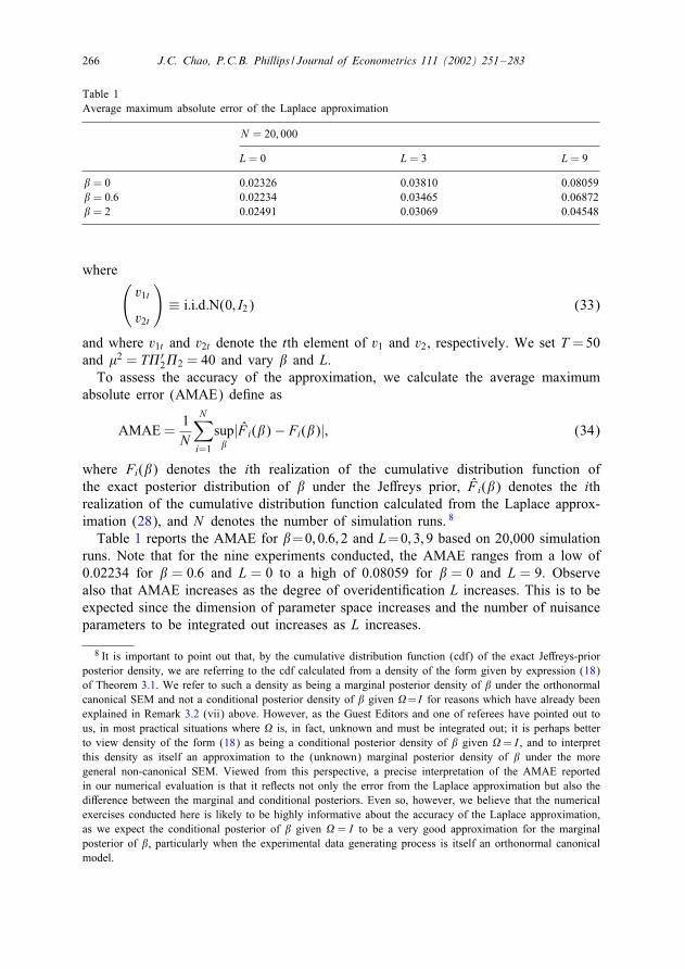
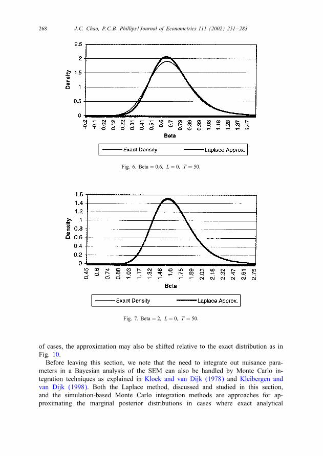
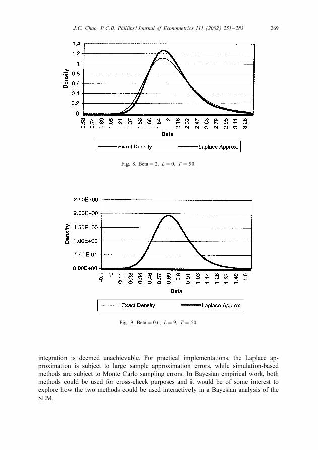
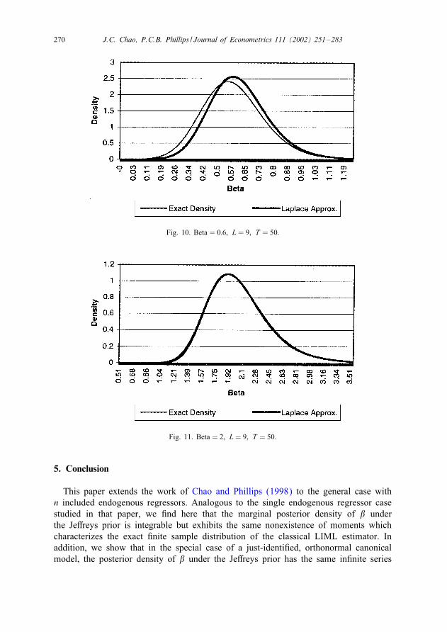
under the Je�reys prior with the Laplace approximation given by expression (28). Thedata generating processes used to generate the graphs are of the same form as that usedfor the simulation above with � taking on the values 0.6 and 2 and L taking on thevalues 0 and 9. Again, we note that a posterior density is a conditional density giventhe data so that its exact outlook will vary depending on the particular data samplethat is drawn. Hence, we provide two graphs for each data generating process used,one illustrating the case where the approximation is very good (Figs. 5, 7, 9 and 11)and another illustrating the case where the approximation is not so good (Figs. 6, 8,10 and 12). Focusing on the cases where the approximation does not perform so well,we see that in most cases the bulk of the approximation error is actually incurred inthe region around the posterior mode (see Figs. 6, 8 and 12) although, in a minority


Fig. 6. Beta = 0:6; L = 0; T = 50.

Fig. 7. Beta = 2; L = 0; T = 50.

of cases, the approximation may also be shifted relative to the exact distribution as inFig. 10.Before leaving this section, we note that the need to integrate out nuisance para-

meters in a Bayesian analysis of the SEM can also be handled by Monte Carlo in-tegration techniques as explained in Kloek and van Dijk (1978) and Kleibergen andvan Dijk (1998). Both the Laplace method, discussed and studied in this section,and the simulation-based Monte Carlo integration methods are approaches for ap-proximating the marginal posterior distributions in cases where exact analytical


Fig. 8. Beta = 2; L = 0; T = 50.

Fig. 9. Beta = 0:6; L = 9; T = 50:

integration is deemed unachievable. For practical implementations, the Laplace ap-proximation is subject to large sample approximation errors, while simulation-basedmethods are subject to Monte Carlo sampling errors. In Bayesian empirical work, bothmethods could be used for cross-check purposes and it would be of some interest toexplore how the two methods could be used interactively in a Bayesian analysis of theSEM.


Fig. 10. Beta = 0:6; L = 9; T = 50:

Fig. 11. Beta = 2; L = 9; T = 50.

5. Conclusion

This paper extends the work of Chao and Phillips (1998) to the general case withn included endogenous regressors. Analogous to the single endogenous regressor casestudied in that paper, we �nd here that the marginal posterior density of � underthe Je�reys prior is integrable but exhibits the same nonexistence of moments whichcharacterizes the exact �nite sample distribution of the classical LIML estimator. Inaddition, we show that in the special case of a just-identi�ed, orthonormal canonicalmodel, the posterior density of � under the Je�reys prior has the same in�nite series


Fig. 12. Beta = 2; L = 9; T = 50.

representation as the exact �nite sample density of LIML derived in Phillips (1980)for that case.The methods employed in this paper come from classical multivariate analysis and

the classical literature on the �nite sample distribution of single-equation estimators.These methods are likely to have applications in Bayesian analysis beyond the con�nesof the present paper. In particular, they are likely to be useful in analyzing the e�ectson posterior inference of applying other types of information-matrix-based priors tothe simultaneous equations model. Indeed, exploring other types of information-matrix-based priors seems an interesting avenue for future research. Research by Kleibergenand van Dijk (1992, 1998), Poirier (1996), and Chao and Phillips (1998) suggests thatthe primary reason why posterior distributions based on the Je�reys prior do not su�erfrom the same pathologies that a�ict di�use-prior posterior distributions is the factthat the Je�reys prior is derived from the information matrix. 9 However, a drawbackof the Je�reys prior in the context of the SEM is that it leads to a posterior densityfor � which has no �nite moments of positive integer order even when the model isoveridenti�ed. It would be nice to �nd a prior which not only preserves the advantagesof the Je�reys prior but also gives rise to posterior tails that are thin enough to allowfor the existence of moments at least up to the degree of overidenti�cation. In thisregard, the alternative information-matrix-based priors proposed by Bernardo (1979),Tibshirani (1989), Berger and Bernardo (1992), and Kleibergen and van Dijk (1998)emerge as interesting possibilities, although further research on these priors in thecontext of the SEM is obviously needed.

9 See Kleibergen and van Dijk (1998) for a discussion of the various pathologies which a�ict thedi�use-prior Bayesian analysis of the simultaneous equations model.


Acknowledgements

The authors thank the Guest Editors, Richard Smith and Peter Boswijk, and twoanonymous referees for many helpful comments and suggestions on earlier drafts ofthis paper. Thanks also go to Harry Kelejian, Herman van Dijk, Marc Nerlove, andIngmar Prucha and participants of the December 1997 EC2 in Amsterdam as well asworkshop participants at the Institute of Economics, Academia Sinica; National TaiwanUniversity; and the University of Maryland for comments on the paper. Any remainingerrors are our own. Phillips thanks the NSF for research support under Grant Nos. SBR94-22922 and SBR 97-30295. The paper was typed by the authors in SW3.0.

Appendix

Proof of Theorem 3.1. We �rst show expression (18). To proceed, we combine theJe�reys prior density (17) with the likelihood function implied by Eqs. (9) and (10)under conditions (7), (11), and (14) to obtain the joint posterior density

p(�; �;�1; �2|Y; Z)˙ |1 + �′�|(1=2)(k2−n)|T�′2�2|1=2

×exp(−12tr[(v1; V2)′(v1; V2)]

): (A.1)

To compute the marginal posterior density of �, we need to integrate (A.1) withrespect to �;�1, and �2. To proceed, note that the posterior density (A.1) can befactorized as follows:

p(�; �;�1; �2|Y; Z)

˙ T−k1=2exp(−12tr[T (�− �̃)′(�− �̃)]

)}(A)

× |TIk1 ⊗ In|−1=2exp(−12tr[T (�1 − �̃1)′(�1 − �̃1)

])}(B)

× |T�′2�2|1=2exp

(−12tr[T (B′

1B1)(�2 − �̃2)′(�2 − �̃2)])}

(C)

×|1 + �′�|(1=2)(k2−n)exp(12tr[T (B′

1B1)�̃′2�̃2

])

×exp(−12[y′

1Qz1y1])

×exp(−12tr[Y ′

2QZ1Y2])

; (A.2)


where

�̃= T−1Z ′1[y1 − Z1�1�];

�̃1 = T−1Z ′1Y2;

�̃2 = T−1Z ′2YB1(B′

1B1)−1:

Note that (A); (B), and (C) are, respectively, proportional to the conditional posteriordensity of � given (�;�1; �2), the conditional posterior density of �1 given (�;�2),the conditional posterior density of �2 given �. Moreover, note that we can easilyintegrate (A.2) with respect to � and �1 since (A) is proportional to the p.d.f. of amultivariate normal distribution while (B) is proportional to that of a matric-variatenormal distribution.To integrate (C) with respect to �2, we proceed as in the derivation of the density

function of the noncentral Wishart distribution (cf. Muirhead, 1982). Write M=T 1=2�2.It follows that d�2 = |T 1=2Ik2 |−n dM so that∫

Rk2n|T�′

2�2|1=2 exp(−12tr[T (B′

1B1)(�2 − �̃2)′(�2 − �̃2)])

(d�2)

=∫Rk2n

|M ′M |1=2 exp(−12tr[(B′

1B1)(M − M̃)′(M − M̃)])

×|T 1=2Ik2 |−n(dM); (A.3)

where M̃=T 1=2�̃2 and where (d�2) and (dM) denote the exterior products of the k2nelements of d�2 and dM as described in Muirhead (1982). To evaluate the right-handside of (A.3), we further write M=H1L, where H1 is a k2×n matrix such that H ′

1H1=Inand where L is upper triangular. Moreover, by Theorem 2.1.14 of Muirhead (1982),the measure (dM) decomposes as follows:

(dM) = 2−ndet(M ′M)(k2−n−1)=2(d(M ′M))(H ′1 dH1); (A.4)

where (d(M ′M)) is the measure on the positive de�nite matrix M ′M and (H ′1 dH1) is

the measure on the matrix of orthogonal columns of H1. Note that

M ′M = L′H ′1H1L= L′L= A (say): (A.5)

Making use of (A.4) and (A.5), we can rewrite the right-hand side of (A.3) as∫A¿0

∫H1∈Vn; k2

|T 1=2Ik2 |−n2−n|A|(k2−n)=2exp(tr[(B′

1B1)M̃′H1L

])

×exp(−12tr[(B′

1B1)A])exp

(−12tr[(B′

1B1)M̃′M̃])

(H1 dH1)(dA); (A.6)


where Vn;k2 is the Stiefel manifold of k2 × n matrices with orthonormal columns. Theinner integral in (A.6) can, in turn, be evaluated as follows:∫

H1∈Vn; k2

exp(tr[(B′

1B1)M̃′H1L

])(H1 dH1)

=�k2−n[ 12 (k2 − n)]2(k2−n)�(k2−n)2=2

×∫H1∈Vn;k2

∫J∈O(k2−n)

exp(tr[(B′

1B1)M̃′H1L

])(K ′ dK)(H1 dH1)

=�k2−n[ 12 (k2 − n)]2(k2−n)�(k2−n)2=2

∫H∈O(k2)

exp(tr[(B′

1B1)M̃′H1L

])(H dH)

=2n�k2n=2

�n( 12k2)

∫O(k2)

exp(tr[(B′

1B1)M̃′H1L

])(dH)

=2n�k2n=2

�n( 12k2)0F1

(12k2;

14L(B′

1B1)M̃′M̃ (B′

1B1)L′)

=2n�k2n=2

�n( 12k2)0F1

(12k2;

12(B′

1B1)M̃′M̃ (B′

1B1)A)

; (A.7)

where O(k2−n) denotes the orthogonal group of (k2−n)×(k2−n) matrices and where

(dH) =1

Vol[O(k2)](H ′ dH):

The second and the fourth equality above follow in a standard way, e.g. see Lemma9.5.3 and Theorem 7.4.1 of Muirhead (1982) respectively. Now, using (A.7) in (A.6),we obtain∫

A¿0

�k2n=2

�n( 12k2)exp

(−12tr[(B′

1B1)M̃′M̃])

×|A|(k2−n)=2exp(−12tr[(B′

1B1)A])

×0F1

(12k2;

14(B′

1; B1)M̃′M̃ (B′

1B1)A)(d A): (A.8)

Finally, the integral (A.8) can be evaluated by noting that the matrix argument hy-pergeometric function 0F1(·) can be given an in�nite series representation in terms ofzonal polynomials as follows:

0F1

(12k2;

14(B′

1B1)M̃′M̃ (B′

1B1)A)

=∞∑j=0

∑J

CJ

(14 (B

′1B1)M̃

′M̃ (B′

1B1)A)

( 12k2)J (j!); (A.9)


where the series is absolutely convergent (e.g., Constantine, 1963). In view of (A.9),we can integrate the integrand of (A.8) term-by-term using Theorem 7.2.7 of Muirhead(1982) to obtain

K0exp(−12tr[(B′

1B1)M̃′M̃])

|B′1B1|−(1=2)(k2+1)

×1F1

(12(k2 + 1);

12k2;

12(B′

1B1)M̃′M̃)

; (A.10)

where

K0 = 2(1=2)(k2+1)�k2n=2�n

(12(k2 + 1)

)/�n

(12k2

):

Note further that

(B′1B1)M̃

′M̃ = T (B′

1B1)�̃′2�̃2

= B′1(Y

′Z2Z ′2Y=T )B1(B′

1B1)−1 (A.11)

and that

|B′1B1|= |In + ��′|: (A.12)

From expressions (A.2) and (A.10)–(A.12), we deduce that

p(�|Y; Z)˙ |1 + �′�|(1=2)(k2−n)exp(12tr[T (B′

1B1)�̃′2�̃2

])

×exp(−12y′1QZ1y1

)exp

(−12tr[Y ′

2QZ1Y2])

×exp(−12tr[(B′

1B1)M̃′M̃])

×|B′1B1|−(1=2)(k2+1)

1F1

(12(k2 + 1);

12k2;

12(B′

1B1)M̃′M̃)

˙ |1 + �′�|−(1=2)(n+1)

×1F1

(12(k2 + 1);

12k2;

12B′1(Y

′Z2Z ′2Y=T )B1(B′

1B1)−1)

(A.13)

as required by expression (18).To show (19), we note that for the just-identi�ed case, k2 = n. Moreover, in this

case

B′1(Y

′Z2Z ′2Y=T )B1(B′

1B1)−1

=(Y ′2Z2 + �y′

1Z2)(1=T )(Z ′2Y2 + Z ′

2y1�′)(In + ��′)−1; (A.14)


but (A.14) has the same eigenvalues as

(1=T )(Z ′2Y2 + Z ′

2y1�′)(In + ��′)−1(Y ′2Z2 + �y′

1Z2)

=T (Z ′2Y2=T )(In + (Z ′

2Y2)−1Z ′2y1�′)(In + ��′)−1

×(In + �y′1Z2(Y ′

2Z2)−1)(Y ′2Z2=T )

=T�̂2(In + �̂2SLS�′)(In + ��′)−1(In + ��̂

′2SLS�̂

′2); (A.15)

where we have made use of the fact that under just identi�cation Z ′2Y2 is nonsingular

almost surely. It follow, then, in this case

1F1

(12(k2 + 1);

12k2;

12B′1(Y

′Z2Z ′2Y=T )B1(B′

1B1)−1)

=1F1

(12(n+ 1);

12n;

T2�̂2(In + �̂2SLS�

′)(In + ��′)−1(In + ��̂′2SLS)�̂

′2

)(A.16)

which establishes expression (19).

Proof of Corollary 3.3. We start with the marginal posterior density of � as given by(18). We want to show that along each ray of the form �= b�0 for some �xed vector�0 �= 0 and some scalar b which tends to in�nity, we have

|1 + b2�′0�0|−(1=2)(n+1)

×1F1

(12(k2 + 1);

12k2;

12(b�0; In)(Y ′Z2Z ′

2Y=T )(b�0; In)′

× ((b�0; In)(b�0; In)′)−1)

=C|1 + b2�′0�0|−(1=2)(n+1)(1 + o(1)); (A.17)

as b → ∞, where

C = 1F1

(12(k2 + 1);

12k2;

12D)

:

Here,

D =

( 11 − ′

21R2

−R′2 21 R′

2 22R2

);

where

11 = y′1Z2Z ′

2y1=T;

21 =−Y ′2Z2Z ′

2y1=T;

22 = Y ′2Z2Z ′

2Y2=T;

and where we de�ne R = (r1; R2) = (�0(�′0�0)−1=2; �0;⊥(�′

0;⊥�0;⊥)−1=2)∈O(n) so that�′0r1 = 1 and �′

0R2 = 0.


To show (A.17), it su�ces to show that

limb→∞ 1F1

(12(k2 + 1);

12k2;

12S(b)

)= C: (A.18)

To show (A.18), de�ne the (n+ 1)× (n+ 1) diagonal matrix

G =

(1b 0

0 In

);

and write

S1(b) =GR′(b�0; In)(Y ′Z2Z ′2Y=T )(b�0; In)′RG

×(GR′(b�0; In)(b�0; In)′RG)−1:

Now, note that

1F1

(12(k2 + 1);

12k2;

12S(b)

)= 1F1

(12(k2 + 1);

12k2;

12S1(b)

)∀b

since S(b) and S1(b) have the same set of eigenvalues. Hence, we can alternativelyshow that

limb→∞ 1F1

(12(k2 + 1);

12k2; S1(b)

)= C:

To proceed, note that with some straightforward algebra, we obtain

S1(b) =

( 11 − ′

21r1=b− r′1 21=b+ r′1 22r1=b2 − ′

21R2 + r′1 22R2=b

−R′2 21 + R′

2 22r1=b R′2 22R2

)

×(1 + 1=b2 0

0 In−1

)−1

→D as b → ∞:

Next, observe that since the eigenvalues of S1(b) are continuous functions of the vari-ates of S1(b) and since the hypergeometric function 1F1(·) is continuous with respectto the eigenvalues of its matrix argument, it follows by continuity that

limb→∞1F1

(12(k2 + 1);

12k2;

12S1(b)

)= 1F1

(12(k2 + 1);

12k2;

12D)

=C; (A.19)

which establishes the desired results (A.17).

Proof of Theorem 4.1. We prove this theorem in two stepsStep 1: We want to show that the conditional posterior density of � given � has no

�nite absolute moments of positive integer order from which it follows by the TonelliTheorem that the marginal posterior density of � also has no �nite absolute moments ofpositive integer order. As this step follows from arguments very similar to those given


in the proofs of Theorem 3.1 and Corollary 3.3 above, we will only brie�y outline theargument.To begin, we note that proceeding as in the proof of Theorem 3.1, we can show

that

p(�|�; Y; Z)

˙ |!11 − 2!′21� + �′�22�|−(1=2)(n+1)

×1F1

(12(k2+1);

12k2;

12B′1�

−1Y ′(PZ−PZ1 )Y�−1B1(B′

1�−1B1)−1

): (A.19)

Next, by following arguments similar to those in the proof of Corollary 3.3, wecan show that along each ray of the form � = b�0 for some �xed vector �0 �= 0 andsome scalar b which tends to in�nity, the limiting behavior of the conditional posteriordensity (A.19) is of the form:

|!11 − 2b!′21�0 + b2�′

0�22�0|−(1=2)(n+1)

×1F1

(12(k2 + 1);

12k2;

12(b�0; In)�−1Y ′(PZ − PZ1 )Y�

−1(b�0; In)′

× ((b�0; In)�−1(b�0; In)′)−1)

=C0|!11 − 2b!′21�0 + b2�′

0�22�0|−(1=2)(n+1)(1 + o(1)); (A.20)

as b → ∞, where

C0 = 1F1

(12(k2 + 1);

12k2;

12D0

)and where

D0 =

(’11 −’′

21R2

−R′2’21 R′

2’22R2

)(!−1

11:2 −!′21�

−122 R2!−1

11:2

−!−111:2R

′2�

−122 !21 R′

2�−122 R2

)−1

;

with ’11; ’21, and ’22 de�ned as follows:

’11 = !−211:2(y1 − Y2�−1

22 !21)′(PZ − PZ1 )(y1 − Y2�−122 !21);

’21 = !−211:2(y1!′

21�−122 − Y2�−1

22:1!11:2)′(PZ − PZ1 )(y1 − Y2�−122 !21);

’22 = !−211:2(y1!′

21�−122 − Y2�−1

22:1!11:2)′(PZ − PZ1 )(y1!′21�

−122 − Y2�−1

22:1!11:2):

As before, de�ne R=(r1; R2)=(�0(�′0�0)−1=2; �0;⊥(�′

0;⊥�0;⊥)−1=2)∈O(n) so that �′0r1=1

and �′0R2 = 0.

Note that the tail behavior of the right-hand side of (A.20) is determined by thefactor

|!11 − 2b!′21�0 + b2�′

0�22�0|−(1=2)(n+1);

which is proportional to the probability density function of a multivariate Cauchy dis-tribution. From this, we deduce that the conditional posterior density of � given � has


no �nite absolute moments of positive integer order. As noted before, it then followsby the Tonelli Theorem that the marginal posterior density of � also has no �niteabsolute moments of positive integer order.Step 2: We need to show that the marginal posterior density of � under the Je�reys

prior is integrable.

To do this, note �rst that given the triangular structure of the SEM described inSection 2 and given the invariance of the Je�reys prior to 1:1 parameter transforma-tion, we will obtain the same marginal posterior density of � regardless of whetherwe proceed from the parameterization given by expressions (9) and (10) under errorcondition (7) or the parameterization given by expressions (1) and (2) under errorcondition (3). Here, we �nd it convenient to proceed from the latter parameterization.Moreover, we make the additional transformation (�11; �21; �22) → (�11; �−1

11 �′21; �22:1)

with Jacobian term |�11|n and write the joint posterior density under the Je�reys priorin the form

p(�; �;�1; �2; �11; �−111 �′

21; �22:1|Y; Z)˙ |�11|−(1=2)(T+k1+2)|�22:1|−(1=2)(T+k+n+2)|�′

2Z′2QZ1Z2�2|1=2

×exp(−12

[�−111 u′u+ tr

(�−122:1V

′2QuV2

)

+ tr(�−122:1(�

−111 �′

21 − (u′u)−1u′V2)′(u′u)(�−111 �′

21 − (u′u)−1u′V2))])

: (A.21)

Next, observe that the conditional posterior density of �−111 �′

21 given all the other para-meters is proportional to the p.d.f. of a multivariate normal. Hence, we can integratewith respect to �−1

11 �′21 to obtain

p(�; �;�1; �2; �11; �22:1|Y; Z)˙ |�11|−(1=2)(T+k1+2)|�22:1|−(1=2)(T+k+n+1)|�′

2Z′2QZ1Z2�2|1=2

×|u′u|−(1=2)nexp(−12

[�−111 u′u+ tr

(�−122:1V

′2QuV2

)]): (A.22)

Moreover, note that the conditional posterior density of �11 given (�; �;�1; �2; �22:1)and that of �22:1 given (�; �;�1; �2) are both that of an inverted Wishart distribution,so we integrate with respect to �11 and �22:1, in turn, to obtain

p(�; �;�1; �2; |Y; Z)˙ |u′u|−(1=2)(T+k1+n)|V2QuV2|−(1=2)(T+k)|�′

2Z′2QZ1Z2�2|1=2

=|u′u|−(1=2)(T+k1+n)|�′2Z

′2QZ1Z2�2|1=2|(Y2 − Z2�2)′Q(u;Z1)(Y2 − Z2�2)

+(�1 − �̂1)′Z ′1QuZ1(�1 − �̂1)|−(1=2)(T+k); (A.23)

where �̂1=(Z ′1QuZ1)−1Z ′

1Qu(Y2−Z2�2). From (A.23), it is apparent that the conditionalposterior density of �1 given (�; �;�2) is that of a matric-variate t distribution which


can be integrated to obtain, after some algebra,

p(�; �;�2; |Y; Z)˙ |u′u|−(1=2)(T+k1)|u′QZ1u|(1=2)(T+k2−n)|u′Q(Y2−Z2�2 ;Z1)u|−(1=2)(T+k2)

×|(Y2 − Z2�2)′QZ1 (Y2 − Z2�2)|−(1=2)(T+k2)|�′2Z

′2QZ1Z2�2|1=2

= |(y1 − Y2�)′QZ1 (y1 − Y2�) + (�− �̂)′Z ′1Z1(�− �̂)|−(1=2)(T+k1)

×|(y1 − Y2�)′QZ1 (y1 − Y2�)|(1=2)(T+k2+n)

×|(y1 − Y2�)′Q(Y2−Z2�2 ;Z1)(y1 − Y2�)|−(1=2)(T+k2)

×|(Y2 − Z2�2)′QZ1 (Y2 − Z2�2)|−(1=2)(T+k2)|�′2Z

′2QZ1Z2�2|1=2; (A.24)

where �̂ = (Z ′1Z1)−1Z ′

1(y1 − Y2�). Once again, we recognize from expression (A.24)that the conditional posterior density of � given (�;�2) is a multivariate t distributionwhich we can integrate to obtain

p(�;�2; |Y; Z)˙ |(y1 − Y2�)′QZ1 (y1 − Y2�)|(1=2)(k2−n)

×|(y1 − Y2�; Y2 − Z2�2)′QZ1 (y1 − Y2�; Y2 − Z2�2)|−(1=2)(T+k2)

×|�′2Z

′2QZ1Z2�2|1=2

= |(y1 − Y2�)′QZ1 (y1 − Y2�)|−(1=2)(T+n)

×|(Y2−Z2�2)′Q(y1−Y2�;Z1)(Y2−Z2�2)|−(1=2)(T+k2)

|�′2Z

′2QZ1Z2�2|1=2: (A.25)

The posterior density of � and �2 cannot be readily integrated with respect to �2 toobtain in closed form the marginal posterior density of �. Instead, we bound (A.25)with an expression for which �2 can be integrated out in closed form and use domi-nated convergence. To proceed, note that for Rank(�2) = n6 k2,

|(y1 − Y2�)′QZ1 (y1 − Y2�)|−(1=2)(T+n)

×|(Y2 − Z2�2)′Q(y1−Y2�;Z1)(Y2 − Z2�2)|−(1=2)(T+k2)|�′2Z

′2QZ1Z2�2|1=2

= |(y1 − Y2�)′QZ1 (y1 − Y2�)|−(1=2)(T+n)

×|(Y2 − Z2�2)′Q(y1−Y2�;Z1)(Y2 − Z2�2)|−(1=2)(T+k2−1)

×|(Y2 − Z2�2)′QZ1 (Y2 − Z2�2)− (Y2 − Z2�2)′(P(y1−Y2�;Z1) − PZ1 )

×(Y2 − Z2�2)|−(1=2)|�′2Z

′2QZ1Z2�2|1=2

6 |(y1 − Y2�)′QZ1 (y1 − Y2�)|−(1=2)(T+n)

×|(Y2 − Z2�2)′Q(y1−Y2�;Z1)(Y2 − Z2�2)|−(1=2)(T+k2−1)

×[|�′2Z

′2QZ1Z2�2|=|�′

2Z′2Q(y1 ;Y2 ;Z1)Z2�2|]1=2


6 |(y1 − Y2�)′QZ1 (y1 − Y2�)|−(1=2)(T+n)|(Y2 − Z2�2)′Q(y1−Y2�;Z1)

× (Y2 − Z2�2)|−(1=2)(T+k2−1)

[n∏

i=1

k2−n+i

/n∏

i=1

�i

]1=2

; (A.26)

where k2−n+1; : : : ; k2 are the n largest eigenvalues of the matrix Z ′2QZ1Z2 and �1; : : : ;

�n are the n smallest eigenvalues of Z ′2Q(y1 ;Y2 ;Z1)Z2. Note that the �rst inequality above

arises because (Y2 − Z2�2)′(P(y1 ;Y2 ;Z1) − P(y1−Y2�;Z1))(Y2 − Z2�2) is at least positivesemide�nite. The second inequality, on the other hand, makes use of Theorem 15 ofChapter 11, Section 13 of Magnus and Neudecker (1988). Observe that

|�′2Z

′2QZ1Z2�2|=|�′

2Z′2Q(y1 ;Y2 ;Z1)Z2�2|

=|(�′2�2)−1=2�′

2Z′2QZ1Z2�2(�′

2�2)−1=2|=|(�′2�2)−1=2�′

2Z′2Q(y1 ;Y2 ;Z1)

Z2�2(�′2�2)−1=2|

6

[n∏

i=1

k2−n+i

/n∏

i=1

�i

]

by Theorem 15 of Magnus and Neudecker (1988). Note further that the upper boundwe achieve in (A.26) can be integrated in closed form with respect to �2 since the solefactor containing �2 in this expression is proportional to the p.d.f. of a matric-variatet distribution. Performing this integration, we obtain an expression proportional to

|(y1 − Y2�)′QZ1 (y1 − Y2�)|−(1=2)(T+n)

×|Y ′2Q(y1−Y2�;Z1 ;Z2)Y2|−(1=2)(T−1)|Z ′

2Q(y1−Y2�;Z1)Z2|−(1=2)n

[n∏

i=1

k2−n+i

/n∏

i=1

�i

]1=2

= C1

[ |(y1 − Y2�)′Q(Z1 ;Z2)(Y1 − Y2�)||(y1 − Y2�)′QZ1 (y1 − Y2�)|

](1=2)T

×|y′1Q(Y2 ;Z1 ;Z2)y1 + (� − �̂)′Y ′

2Q(Z1 ;Z2)Y2(� − �̂)|−(1=2)(n+1)

6C1|y′1Q(Y2 ;Z1 ;Z2)y1 + (� − �̂)′Y ′

2Q(Z1 ;Z2)Y2(� − �̂)|−(1=2)(n+1); (A.27)

where

C1 =

[n∏

i=1

k2−n+i

/n∏

i=1

�i

]1=2

|y′1Q(Y2 ;Z1 ;Z2)y1|−(1=2)(T−1)

×|Y ′2Q(Z1 ;Z2)Y2|−(1=2)(T−1)|Z ′

2QZ1Z2|−(1=2)n;

where

�̂ = (Y ′2Q(Z1 ;Z2)Y2)−1Y ′

2Q(Z1 ;Z2)y1;

and where the inequality follows from the positive de�niteness of Y ′(QZ1 −Q(Z1 ;Z2))Y =Y ′(PZ−PZ1 )Y . Finally, observe that the right-most expression of (A.27) is proportional


to the p.d.f. of a multivariate Cauchy distribution and is, thus, integrable with respectto �. From this, we deduce the integrability of the marginal posterior density of �under the Je�reys prior.

References

Basmann, R.L., 1974. Exact �nite sample distributions for some econometric estimators and test statistics: asurvey and appraisal (with discussion). In: Intriligator, M.D., Kendrick, D. (Eds.), Frontiers of QuantitativeEconomics. North-Holland, Amsterdam, pp. 209–288.

Berger, J., Bernardo, J.M., 1992. Reference priors in a variance components problem. In: Goel, P., Iyengar,N.S. (Eds.), Bayesian Analysis in Statistics and Econometrics. Springer, New York, pp. 177–194.

Bernardo, J.M., 1979. Reference posterior distributions for Bayesian inference. Journal of the Royal StatisticalSociety, Series B 41, 113–147.

Chao, J.C., Phillips, P.C.B., 1998. Posterior distributions in limited information analysis of the simultaneousequations model using the Je�reys prior. Journal of Econometrics 87, 49–86.

Constantine, A.G., 1963. Some noncentral distribution problems in multivariate analysis. Annals ofMathematical Statistics 34, 1270–1285.

Dr�eze, J.H., 1976. Bayesian limited information analysis of the simultaneous equations model. Econometrica44, 1045–1075.

James, A.T., 1968. Calculation of zonal polynomials coe�cients by use of the Laplace–Beltrami operator.Annals of Mathematical Statistics 39, 1711–1718.

Je�reys, H., 1946. An invariant form for the prior probability in estimation problems. Proceedings of theRoyal Society of London, Series A 186, 453–461.

Je�reys, H., 1961. Theory of Probability, 3rd Edition. Oxford University Press, London.Kass, R.E., 1989. The geometry of asymptotic inference. Statistical Science 4, 188–234.Kleibergen, F.R., van Dijk, H.K., 1992. Bayesian simultaneous equation model analysis: on the existence of

structural posterior moments. Working paper no. 9269/A, Erasmus University, Rotterdam.Kleibergen, F.R., van Dijk, H.K., 1994. On the shape of likelihood/posterior in cointegration models.

Econometric Theory 10, 514–551.Kleibergen, F.R., van Dijk, H.K., 1998. Bayesian simultaneous equations analysis using reduced rank

structures. Econometric Theory 14, 701–743.Kleibergen, F.R., Zivot, E., 2000. Bayesian and classical approaches to instrumental variable regression.

Journal of Econometrics, forthcoming.Kloek, T., van Dijk, H.K., 1978. Bayesian estimates of equation system parameters: an application of

integration by Monte Carlo. Econometrica 46, 1–19.Magnus, J.R., Neudecker, H., 1988. Matrix Di�erential Calculus with Applications in Statistics and

Econometrics. Wiley, New York.Mariano, R.S., 1982. Analytical small-sample distribution theory in econometrics: the simultaneous-equations

case. International Economic Review 23, 503–533.Mariano, R.S., McDonald, J.B., 1979. A note on the distribution functions of LIML and 2SLS structural

coe�cient in the exactly identi�ed case. Journal of the American Statistical Association 74, 847–848.McLaren, M.L., 1976. Coe�cients of the zonal polynomials. Applied Statistics 25, 82–87.Muirhead, R.J., 1982. Aspects of Multivariate Statistical Theory. Wiley, New York.Nagel, P.J.A., 1981. Programs for the evaluation of zonal polynomials. American Statistician 35, 53.Nicolaou, A., 1993. Bayesian intervals with good frequency behavior in the presence of nuisance parameters.

Journal of the Royal Statistical Society, Series B 55, 377–390.Peers, H.W., 1965. On con�dence points and Bayesian probability points in the case of several parameters.

Journal of the Royal Statistical Society, Series B 27, 9–16.Phillips, P.C.B., 1980. The exact distribution of instrumental variable estimators in an equation containing

n + 1 endogenous variables. Econometrica 48, 861–878.Phillips, P.C.B., 1983. Exact small sample theory in the simultaneous equations model. In: Intriligator, M.D.,

Griliches, Z. (Eds.), Handbook of Econometrics. North-Holland, Amsterdam, pp. 449–516.


Phillips, P.C.B., 1984. The exact distribution of LIML: I. International Economic Review 25, 249–261.Phillips, P.C.B., 1985. The exact distribution of LIML: II. International Economic Review 26, 21–36.Phillips, P.C.B., 1989. Partially identi�ed econometric models. Econometric Theory 5, 181–240.Phillips, P.C.B., 1991. To criticize the critics: an objective Bayesian analysis of stochastic trends. Journal of

Applied Econometrics 6, 333–364.Phillips, P.C.B., 1994. Some exact distribution theory for maximum likelihood estimators of cointegrating

coe�cients in errors correction models. Econometrica 62, 73–94.Poirier, D., 1994. Je�reys prior for logit models. Journal of Econometrics 63, 327–339.Poirier, D., 1996. Prior beliefs about �t. In: Bernardo, J.M., Berger, J.O., Dawid, A.P., Smith, A.F.M. (Eds.),

Bayesian Statistics, Vol. 5. Clarendon Press, Oxford, pp. 731–738.Tibshirani, R., 1989. Noninformative priors for one parameter of many. Biormetrika 76, 604–608.Welch, B.L., Peers, H.W., 1963. On formulae for con�dence points based on integrals of weighted likelihoods.

Journal of the Royal Statistical Society, Series B 35, 318–329.Zellner, A., 1970. Estimation of regression relationships containing unobservable independent variables.

International Economic Review 11, 441–454.Zellner, A., 1971. An Introduction to Bayesian Inference in Econometrics. Wiley, New York.

jeffreys prior analysis of the simultaneous

Documents