jayson mcallister - university of albertajinfeng/thesis/2017_jayson_mcallister... · chronic kidney...
TRANSCRIPT
Modeling and Control of Hemoglobin for Anemia Management inChronic Kidney Disease
by
Jayson McAllister
A thesis submitted in partial fulfillment of the requirements for the degree of
Master of Science
in
Process Control
Department of Chemical and Materials Engineering
University of Alberta
c©Jayson McAllister, 2017

Abstract
Chronic Kidney Disease (CKD) affects millions of people throughout the world
today. One of the major side effects of this disease is the inability to regulate the
body’s red blood cell production, and subsequently the mass of the protein called
hemoglobin within the body. The health of these patients deteriorates and they be-
come anemic. Recently, erythropoietin stimulating agents have become the standard
for treating anemia in chronic kidney disease. The medication works extremely well
for what it is designed to do. The problem with this scenario is the inability of the
physician’s to be able to choose an appropriate dose for each patient. The dosing
protocols are not standardized across hospitals, and many of the dosing regimens are
poorly designed. As such, many patients’ hemoglobin levels are poorly controlled.
The poor control of hemoglobin in CKD patients is well documented through peer
reviewed research. The focus of this thesis is to present an individualized epoetin-alfa
dosing regimen, through the use of well known model predictive control technologies.
Due to the absence of a proper setpoint, zone model predictive control becomes the
focus of the controller methods.
The foundation of any model predictive controller is the system model. This thesis
presents several different hemoglobin response modeling techniques including classical
ARX, pharmacokinetic and pharmacodynamic (PKPD) delayed differential equation
modeling and a novel new nonlinear constrained ARX modeling (C-ARX) method.
The hemoglobin response modeling methods are compared on a clinical data set of
167 patients. It will be shown that the new modeling method offers similar modeling
results to the previously developed PKPD model, with the added benefit of being
linear and easily estimated through nonlinear programming. The nonlinear C-ARX
method is also converted to a weighted linear C-ARX, which improves the robustness
of estimation even further, without a large loss in estimation performance.
ii
Different model predictive controllers were tested against the current anemia man-
agement protocol (AMP) from a participating hospital. The first set of tests were
performed using the identified models as the simulated patient and represent a more
nominal case for controller testing. Using these results, some of the controllers were
eliminated from further testing. The second set of simulations were performed on a
patient simulator that was designed based on the PKPD models. The simulator uses
random integrating process noise to represent a slowly changing dose over time. The
designed simulator also incorporates random step and ramp disturbances to simulate
blood loss, infections and other acute anomalies observed in the clinical data. The
remaining controller types were tested on the designed patient simulator and repre-
sent a realistic and rigorous test scenario for the modeling and control methods. The
final controller recommended for use is a weighted recursive least squares zone model
predictive controller that uses a funnel shaped control zone.
iii

Acknowledgements
First and foremost, I’d like to thank my supervisors Dr. Jinfeng Liu and Dr.
Zukui Li of the Chemical and Material Engineering Department at the University of
Alberta. Without their guidance, this thesis would not have been possible. Both Dr.
Liu and Dr. Li contributed unique aspects of their knowledge to aid in guiding me
on the creation of this thesis. Without Dr. Li, the constrained optimization ARX
method would not be a reality. I value his infinite wisdom in the field of optimization
and taking the time to share his knowledge with me as I used complex optimization
techniques in both the modeling and control aspects of the project. I thank Dr.
Liu for providing a great deal of support in regards to the entire hemoglobin control
project. His broad and detailed knowledge of control theory was extremely useful,
and he seemed to always have new and better ideas when I came upon roadblocks in
my research. I have learned so much in these two short years as a result of both of
their hard work and dedication to me, and I will be forever grateful to them.
I also owe a great deal of thanks to the individuals and organizations that provided
funding to allow me to research this project. This includes the University of Alberta
Faculty of Graduate Studies and Research and the Graduate Student’s Association
for the contribution of travel assistance to allow me to present my research at the
American Institute of Chemical Engineers conference in San Francisco, USA. I thank
the Natural Sciences and Engineering Research Council of Canada for funding for
this research. I thank Cybernius Medical Ltd. for their monetary contribution, as
well as their knowledge and clinical data used on this project. I must also thank
the International Society of Automation for the generous scholarship I received from
them.
I’d like to thank Dr. Li, Dr. Liu and Dr. Stevan Dubljevic for the opportunity
to become a teaching assistant in their classes. They say you do not truly know
iv

something until you can teach it to someone else. Being a TA allowed me to refresh
on some important control courses and also allowed me to teach and meet many of
the bright future leaders of tomorrow.
Last but not least, I must thank the other graduate students who have contributed
significantly to my progress. These include Su Liu, Tianrui An, Kevin Arulmaran,
Xunyuan Yin and Jannatun Nahar. I wish them all the best in their future endeavors
v

Contents
1 Introduction 1
1.1 Motivation . . . . . . . . . . . . . . . . . . . . . . . . . . . . . . . . . 1
1.2 Thesis Outline and Contributions . . . . . . . . . . . . . . . . . . . . 3
2 System Identification for Hemoglobin Response Models 5
2.1 Introduction . . . . . . . . . . . . . . . . . . . . . . . . . . . . . . . . 5
2.2 Data Preprocessing for ARX Modeling . . . . . . . . . . . . . . . . . 5
2.3 Modeling Techniques . . . . . . . . . . . . . . . . . . . . . . . . . . . 6
2.3.1 Autoregressive with Exogenous Inputs Modeling . . . . . . . . 7
2.3.2 Pharmacokinetic and Pharmacodynamic Modeling . . . . . . . 10
2.3.3 Constrained Autoregressive with Exogenous Inputs (C-ARX)
Modeling . . . . . . . . . . . . . . . . . . . . . . . . . . . . . 18
2.3.4 Linear C-ARX Modeling . . . . . . . . . . . . . . . . . . . . . 21
2.4 Modeling Results on Clinical Data . . . . . . . . . . . . . . . . . . . . 23
2.4.1 Model Order Reduction . . . . . . . . . . . . . . . . . . . . . 29
2.4.2 Recursive Linear ARX Modeling Results . . . . . . . . . . . . 31
2.5 Conclusions . . . . . . . . . . . . . . . . . . . . . . . . . . . . . . . . 32
3 Hemoglobin Controller Designs 35
3.1 Introduction . . . . . . . . . . . . . . . . . . . . . . . . . . . . . . . . 35
3.2 System Model . . . . . . . . . . . . . . . . . . . . . . . . . . . . . . . 38
3.3 Deterministic Model Predictive Controller Designs . . . . . . . . . . . 38
3.3.1 Zone MPC Cost Function and Reformulation of Problem into
Quadratic Program . . . . . . . . . . . . . . . . . . . . . . . . 38
3.3.2 Classical Model Predictive Control (MPC) . . . . . . . . . . . 41
vi

3.3.3 Zone Model Predictive Control (ZMPC) . . . . . . . . . . . . 41
3.3.4 Economic Model Predictive Control (EMPC) . . . . . . . . . . 44
3.3.5 Nonlinear Zone MPC . . . . . . . . . . . . . . . . . . . . . . . 46
3.4 Stochastic Model Predictive Controller Designs . . . . . . . . . . . . 47
3.4.1 Stochastic System Model . . . . . . . . . . . . . . . . . . . . . 48
3.4.2 Chance Constraints with Gaussian Uncertainty . . . . . . . . 48
3.4.3 Conditional Value at Risk (CVaR) Constraints . . . . . . . . . 49
3.4.4 Zone MPC Hybrid Controller using Hard Chance Constraints 52
3.4.5 Zone MPC using Soft Chance Constraints . . . . . . . . . . . 52
3.4.6 Scenario Based Zone MPC using Hard CVaR Constraints . . . 54
3.4.7 Scenario Based Zone MPC using Soft CVaR Constraints . . . 56
3.4.8 Scenario Based Zone MPC using Conditional Value at Risk in
Cost Function . . . . . . . . . . . . . . . . . . . . . . . . . . . 57
3.5 Time-varying System Controllers for Disturbance Rejection and Offset-
Free Control . . . . . . . . . . . . . . . . . . . . . . . . . . . . . . . . 59
3.5.1 ZMPC with Internal Model Control and Integrator . . . . . . 60
3.5.2 ZMPC with Recursive Modeling . . . . . . . . . . . . . . . . . 62
3.5.3 Digital PID Control . . . . . . . . . . . . . . . . . . . . . . . . 64
3.6 Conclusion . . . . . . . . . . . . . . . . . . . . . . . . . . . . . . . . . 66
4 Simulation Results and Discussion 67
4.1 Introduction . . . . . . . . . . . . . . . . . . . . . . . . . . . . . . . . 67
4.2 Simulation Results using Identified ARX Models to Simulate Patients 68
4.2.1 MPC Tuning . . . . . . . . . . . . . . . . . . . . . . . . . . . 68
4.2.2 Additive Process Noise Simulation Results . . . . . . . . . . . 78
4.2.3 Disturbance Rejection . . . . . . . . . . . . . . . . . . . . . . 81
4.3 Controller Simulation Results on PK/PD Patient Simulator . . . . . 86
4.3.1 Patient Simulator Design . . . . . . . . . . . . . . . . . . . . . 86
4.3.2 Process and Measurement Noise . . . . . . . . . . . . . . . . . 91
4.3.3 Simulation Results on PK/PD Simulator . . . . . . . . . . . . 92
4.4 Conclusion . . . . . . . . . . . . . . . . . . . . . . . . . . . . . . . . . 106
vii

5 Future Work 108
5.1 Introduction . . . . . . . . . . . . . . . . . . . . . . . . . . . . . . . . 108
5.1.1 Patient Simulator . . . . . . . . . . . . . . . . . . . . . . . . . 108
5.1.2 Process Model Improvement . . . . . . . . . . . . . . . . . . . 109
5.1.3 Advanced Model Predictive Controllers using Parameter Un-
certainty . . . . . . . . . . . . . . . . . . . . . . . . . . . . . . 109
5.1.4 Self-tuning PID . . . . . . . . . . . . . . . . . . . . . . . . . . 109
viii

List of Tables
2.1 Estimated parameters and descriptions for the PK/PD Model . . . . 11
2.2 Statistics describing the clinical data used in the modeling methods . 24
2.3 Modeling Results of the unfiltered models for the various modeling
methods explored along with the number of models included in the
resulting statistics . . . . . . . . . . . . . . . . . . . . . . . . . . . . . 25
2.4 Modeling Results for the various modeling methods where patients
with validation RMSE ≥ 3 removed from corresponding model type . 27
2.5 Modeling Results without filtering for the various model orders of Con-
strained ARX models . . . . . . . . . . . . . . . . . . . . . . . . . . . 30
2.6 Constrained ARX Modeling Results with filtering out all models with
Validation RMSE ≥ 3 . . . . . . . . . . . . . . . . . . . . . . . . . . 30
2.7 Constrained ARX Modeling Results with filtering out all models with
Validation RMSE ≥ 1 . . . . . . . . . . . . . . . . . . . . . . . . . . 31
2.8 Modeling Results for the 3 C-ARX methods where patients with vali-
dation Mean RMSE ≥ 3 removed from corresponding model type . . 31
2.9 Highlights of the Recursive Modeling 8-Step Residual Statistics for the
Linear C-ARX modeling methods with various settings . . . . . . . . 32
4.1 Final tuning settings for the ZMPC controllers that will be tested . . 69
4.2 Final tuning settings for the ZMPC-CVaR (constraint) controller that
will be tested. . . . . . . . . . . . . . . . . . . . . . . . . . . . . . . 72
4.3 Final tuning settings for the ZMPC-CVaR (Soft Constraint) controller
that will be tested. . . . . . . . . . . . . . . . . . . . . . . . . . . . . 73
4.4 Final tuning settings for the ZMPC-CVaR (cost) controller that will
be tested. . . . . . . . . . . . . . . . . . . . . . . . . . . . . . . . . . 75
ix

4.5 Final tuning settings for the ZMPC-HCC (7) controller that will be
tested. . . . . . . . . . . . . . . . . . . . . . . . . . . . . . . . . . . 76
4.6 Final tuning settings for the ZMPC-SCC (7) controller that will be
tested. . . . . . . . . . . . . . . . . . . . . . . . . . . . . . . . . . . 78
4.7 Simulation Results for the various ZMPC controllers as compared to
the physician’s protocol for the additive process noise test scenario . . 79
4.8 Simulation Results for the various ZMPC controllers as compared to
the physician’s protocol for the designed disturbance test scenario . . 85
4.9 1-Step Residual Statistics . . . . . . . . . . . . . . . . . . . . . . . . 91
4.10 Tuning parameters for the different model predictive controllers explored 97
x

List of Figures
1.1 Actual clinical patients that undergo hemoglobin cycling . . . . . . . 2
2.1 Patient Data Resampling Example . . . . . . . . . . . . . . . . . . . 7
2.2 bk Parameters for a [1 20 1] Population ARX Model, along with one
standard error . . . . . . . . . . . . . . . . . . . . . . . . . . . . . . . 8
2.3 Average Impulse Response for the Filtered and Resampled Clinical
Data with SEM, using a Pre-whitening filter . . . . . . . . . . . . . . 9
2.4 Cross Correlation Values for the filtered and resampled data, shown
with the SEM . . . . . . . . . . . . . . . . . . . . . . . . . . . . . . . 10
2.5 Example of the State Evolution when simulated with the designed DDE
Solver . . . . . . . . . . . . . . . . . . . . . . . . . . . . . . . . . . . 15
2.6 Example of the ARX approximation for the Nonlinear state space for
an infinite step ahead prediction . . . . . . . . . . . . . . . . . . . . . 16
2.7 Example of the bk parameter structure for the PK/PD ARX approxi-
mation . . . . . . . . . . . . . . . . . . . . . . . . . . . . . . . . . . 17
2.8 Average values of the bk parameters in the IR models of all the esti-
mated PKPD-ARX models over 50 lags . . . . . . . . . . . . . . . . 18
2.9 Average values of the bk parameters in the IR models of all the esti-
mated C-ARX models over 50 lags . . . . . . . . . . . . . . . . . . . 21
2.10 Example that shows the ARX modeling methods capturing the peaks
of the data, where as the PKPD model does not capture the sharpness
of the data peaks . . . . . . . . . . . . . . . . . . . . . . . . . . . . . 25
2.11 ARX modeling Algorithm fails to estimate a proper model. Modeling
results for both training and validation data for all modeling methods 26
xi

2.12 Example patient showing the modeling methods robustness for reject-
ing disturbances in the training data . . . . . . . . . . . . . . . . . . 28
2.13 Example of a patient where the health continually deteriorates over
the length of the patient history. . . . . . . . . . . . . . . . . . . . . . 29
3.1 Relationship between Patient Weight and Average EPO dose for 167
clinical patients . . . . . . . . . . . . . . . . . . . . . . . . . . . . . . 36
3.2 Physician’s Protocol for dosing Epoetin-alfa . . . . . . . . . . . . . . 37
3.3 Constraint boundaries for the slack variable δk when the shape tuning
parameter (p) is set to 0.6 . . . . . . . . . . . . . . . . . . . . . . . . 42
3.4 Comparison of Zone MPC with static vs decaying constraints on the
slack variable under nominal conditions . . . . . . . . . . . . . . . . . 43
3.5 Comparison of EMPC with classical MPC for a 100 week patient sim-
ulation using additive process noise drawn from N(0, 0.252) . . . . . 45
3.6 Simulations comparing different tuning parameters for the EMPC con-
troller . . . . . . . . . . . . . . . . . . . . . . . . . . . . . . . . . . . 45
3.7 Example 100 week Simulation for a Nonlinear MPC controller versus
a linear MPC controller for a single patient when trying to control the
PK/PD model with measurement noise and parameter variation . . . 47
3.8 Block Diagram of the MPC and IMC algorithm with a filtered inte-
grator when simulated using a disturbance variable and measurement
noise . . . . . . . . . . . . . . . . . . . . . . . . . . . . . . . . . . . . 61
3.9 Comparison of different filter values with an Offset-Free MPC con-
troller versus a classical MPC controller for a single patient when trying
to control the PK/PD model with uncertainties . . . . . . . . . . . . 62
3.10 Block Diagram of the MPC algorithm with recursive modeling when
simulated using disturbance and measurement noise . . . . . . . . . . 63
3.11 Comparison of Recursive ZMPC and the IMC-MPC configuration for a
single patient when trying to control the PK/PD model with uncertainties 63
3.12 Graphical Approach to estimating a First Order plus Deadtime transfer
function that is used to attain continuous time transfer functions for
PID controller design . . . . . . . . . . . . . . . . . . . . . . . . . . . 65
xii
4.1 Example simulation comparing ZMPC with static boundaries and de-
caying boundaries on the δk constraints . . . . . . . . . . . . . . . . . 69
4.2 Example simulation showcasing the ability of CVaR constraints to reg-
ulate the zone boundary . . . . . . . . . . . . . . . . . . . . . . . . . 70
4.3 Example simulation showcasing that if Q is set too high, the CVaR
constraints have little impact on the solution . . . . . . . . . . . . . . 71
4.4 Example simulation using the final controller tuning settings for the
ZMPC-CVaR (constraints) controller to be tested as compared to clas-
sical MPC . . . . . . . . . . . . . . . . . . . . . . . . . . . . . . . . . 72
4.5 Example simulation using the final controller tuning settings for the
ZMPC-CVaR (Soft Constraint) controller to be tested as compared to
ZMPC with static boundaries . . . . . . . . . . . . . . . . . . . . . . 73
4.6 Example simulation using the final controller tuning settings for the
ZMPC-CVaR (Cost) controller to be tested as compared to ZMPC
with static boundaries . . . . . . . . . . . . . . . . . . . . . . . . . . 74
4.7 Example simulation using the final controller tuning settings for the
ZMPC-HCC (7) to be tested as compared to ZMPC with static bound-
aries . . . . . . . . . . . . . . . . . . . . . . . . . . . . . . . . . . . . 75
4.8 Example simulation using the final controller tuning settings for the
ZMPC-HCC (7) to be tested as compared to ZMPC with static bound-
aries . . . . . . . . . . . . . . . . . . . . . . . . . . . . . . . . . . . . 76
4.9 Example simulation using the final controller tuning settings for the
ZMPC-SCC (7) to be tested as compared to ZMPC with static boundaries 77
4.10 Block Diagram of the MPC controller test simulations using an ARX
model as the patient simulator . . . . . . . . . . . . . . . . . . . . . . 78
4.11 Example simulation of the controller response to the designed output
disturbance # 1 vector for the nominal case (no process noise) . . . . 82
4.12 Example simulation of the controller response to the designed output
disturbance #1 vector along with additive process noise drawn from
the distribution of N(0, 0.252) . . . . . . . . . . . . . . . . . . . . . . 83
4.13 Example simulation of the controller responses to successive negative
step disturbances for the nominal case (no process noise) . . . . . . . 84
xiii

4.14 Example simulation of the controller responses to successive negative
step disturbances along with additive process noise drawn from the
distribution of N(0, 0.252) . . . . . . . . . . . . . . . . . . . . . . . . 85
4.15 Block Diagram of the Simulation Setup for Recursive Zone Model Pre-
dictive Control and the Patient Simulator . . . . . . . . . . . . . . . 87
4.16 Example of a scenario used to attain the C-ARX models from simulated
data . . . . . . . . . . . . . . . . . . . . . . . . . . . . . . . . . . . . 87
4.17 Clinical patients will become continually more dependent on EPO
doses if their natural endogenous erythropoietin production deterio-
rates . . . . . . . . . . . . . . . . . . . . . . . . . . . . . . . . . . . . 88
4.18 Clinical patients become less dependent on EPO doses as their natural
endogenous erythropoietin production increases . . . . . . . . . . . . 88
4.19 Clinical patients’ exhibiting acute disturbances . . . . . . . . . . . . 89
4.20 Block Diagram of the Patient Simulator . . . . . . . . . . . . . . . . 90
4.21 Simulations showcasing the features of the designed patient simulator 91
4.22 1-Step Residuals for all Patients . . . . . . . . . . . . . . . . . . . . . 91
4.23 Comparison of different classical MPC tuning settings . . . . . . . . 93
4.24 Comparison of different window size lengths used for linear constrained
ARX model estimation . . . . . . . . . . . . . . . . . . . . . . . . . . 94
4.25 Comparison of different tuning parameters for the economic term . . 95
4.26 Hemoglobin Offset produced by the economic term . . . . . . . . . . 96
4.27 Comparison of different weighting matrices for the weighted least squares
modeling methods used in tandem with the funnel model predictive
controller . . . . . . . . . . . . . . . . . . . . . . . . . . . . . . . . . 97
4.28 Comparison of different anemia management controllers in the high
noise environment . . . . . . . . . . . . . . . . . . . . . . . . . . . . . 99
4.29 Comparison of different anemia management controllers in the low
noise environment . . . . . . . . . . . . . . . . . . . . . . . . . . . . . 100
4.30 Comparison of different anemia management controllers in the noise
environment without the integrating disturbance . . . . . . . . . . . . 101
4.31 Simulation Results where the current AMP fails to control the patient
Hgb adequately . . . . . . . . . . . . . . . . . . . . . . . . . . . . . . 102
xiv

4.32 Simulation Results showing the importance of recursive modeling, and
a case where R-ZMPC uses much more drug dose than necessary . . . 103
4.33 Simulation Results showing some of the failures of the PID controller 103
4.34 Simulation Results showing some patients that have a decaying/improving
health over time . . . . . . . . . . . . . . . . . . . . . . . . . . . . . . 104
4.35 Simulation Results showing the difficulty for obtaining a one-size-fits-
all set of tuning parameters for economic R-FMPC . . . . . . . . . . 105
4.36 Simulation Results showing the minimal difference between weighted
and non-weighted R-FMPC and the poor performance of the nonlinear
C-ARX method for recursive model estimation . . . . . . . . . . . . . 106
xv

Chapter 1
Introduction
1.1 Motivation
Chronic Kidney Disease (CKD) is estimated to affect nearly 10% of the world’s
population (A. Levey, 2007). There are several stages of CKD that patients can
be categorized into, with the most severe stage being classified as End Stage Renal
Disease (ESRD). Millions of people worldwide are classified as ESRD patients and
many undergo dialysis treatment or kidney transplants as a result (W. Couser, 2011).
Over 80 % of chronic kidney disease patients that receive treatment are in wealthy
countries that have access to universal healthcare and have large elderly populations
(V. Jha, 2013). The elderly population is increasing at a quick rate in developing
countires such as China and India and the number of chronic kidney disease patients
is expected to increase drastically over the coming years (V. Jha, 2013).
One of the major side effects of CKD is the inability to produce endogenous ery-
thropoietin, which is a hormone used to regulate the production of red blood cells in
the body. Red blood cells contain a protein called hemoglobin which is vital to the
survival of a human. Hemoglobin is responsible for binding to oxygen and delivering
it around the body to the tissues and organs. Without oxygen, the organs and tissues
will die. When the natural production of erythropoietin drops significantly, these pa-
tients suffer from a condition called anemia, which is characterized as a reduced mass
of red blood cells and hemoglobin within the body. In the 1980s, recombinant human
erythropoietin (rHuEPO) was shown to help regulate the production of red blood
cells and hemoglobin. It was in this time period that CKD patients suffering from
anemia started to undergo erythropoietin stimulating agent (ESA) treatment. Since
1

the initial discovery of rHuEPO, several drugs have been invented to stimulate the
production of red blood cells and hemoglobin including darbepoetin-alfa, epoetin-alfa
(EPO), epoetin-beta and methoxy polyethylene glycol-epoetin beta.
It has been recognized by the clinical community that while low hemoglobin levels
lead to anemia, hemoglobin values above 13.0 g/dL can increase the risk of mortal-
ity for the patient (Rosner and Bolton, 2008; Jing et al., 2012; Singh et al., 2006).
Hence, effective methods are needed to determine the appropriate dose of ESA to
maintain the target hemoglobin level. Many conventional methods for guiding ESA
and iron dosing used by clinicians, rely on a set of rules based on past experiences
or retrospective studies. Those methods for ESA administration are generally im-
precise, and as a result, the patient’s hemoglobin levels are often poorly controlled.
The hemoglobin often moves through the target range with large oscillations and
overshoots. Of the 167 clinical patients studied, approximately 56% of the patients
depict some varying degree of oscillatory behaviour that lasts for months or years.
This phenomena is shown for several patients in Figure 1.1, where the control zone is
from 9.5 to 11 g/dL. New effective anemia management methods are needed to avoid
the adverse effects associated with increased hemoglobin levels, while minimizing the
effects of anemia. It is estimated that CKD costs the United States 48 billion dollars
per year (National Kidney Foundation, 2017), and utilizes approximately 6.7% of
Medicare’s annual budget to treat a small fraction (< 1%) of the population (Damien
et al., 2016). It becomes clear that major treatment cost savings could be possible,
while also improving the health of CKD patients.
0 100 200 300 400 500 600 700 800 900 1000
Hgb
, (g/
dL)
6
8
10
12
14
Time (days)0 100 200 300 400 500 600 700 800 900 1000
E
PO
(IU
)
0
5000
10000
15000
(a) Patient 1
0 100 200 300 400 500 600 700 800 900 1000
Hgb
, (g/
dL)
6
8
10
12
14
Time (days)0 100 200 300 400 500 600 700 800 900 1000
E
PO
(IU
)
×104
0
2
4
6
(b) Patient 2
0 100 200 300 400 500 600 700 800 900 1000
Hgb
, (g/
dL)
6
8
10
12
14
Time (days)0 100 200 300 400 500 600 700 800 900 1000
E
PO
(IU
)
×104
0
1
2
3
(c) Patient 3
Figure 1.1: Actual clinical patients that undergo hemoglobin cycling
2

1.2 Thesis Outline and Contributions
Chapter 2 begins with a method of data preprocessing that is introduced to re-
sample the patient data into discrete weekly measurements. Three modeling methods
are then introduced in detail including ARX modeling, Pharmacokinetic and Phar-
macodynamic (PK/PD) modeling and nonlinear Constrained ARX modeling. The
modeling methods are performed on the clinical data and the results are presented.
This chapter shows that the new method of Hemoglobin Response modeling developed
through Constrained ARX modeling is the most effective method in predicting patient
hemoglobin. The nonlinear constrained ARX is also simplified into a weighted linear
quadratic program making the optimization of the parameters more robust, without
losing a great deal of model performance as compared to the nonlinear programming
problem. The new linear C-ARX method is used on the clinical data to test the
effectiveness of the model algorithm to recursively estimate models at each sampling
instant. The model performance is based on the 8-step ahead prediction residuals.
Chapter 3 begins with an example of one of the current Anemia Management
Protocols from a participating hospital. Then, a short description of the model struc-
ture used within the model predictive control algorithms is presented. Many different
types of deterministic model predictive controllers are introduced, and subsequently
reformulated in quadratic programs which are quickly and efficiently solved by con-
ventional optimization methods. The next section of this chapter focuses on stochastic
model predictive controllers which take in to account the best known uncertainties
for additive process noise disturbance and measurement noise. This section explores
the theory behind chance constraints and conditional value at risk constraints. The
problems are reformulated into standard quadratic or linear programs. Three con-
troller algorithms are then presented for dealing with time-varying disturbances. The
chapter ends with some concluding remarks about the controller designs explored.
In Chapter 4, controller tuning is discussed in detail for the controllers to be
tested through computer simulations and the results are presented. Simulation results
are presented for the clinical patient models, and the current AMP is compared to
several of the controller options. The controllers were tested using a combination of
additive process noise and measurement noise while using the linear ARX model as
3

the patient simulator. Some of the controllers were then tested on a Patient Simulator
that was designed based on the PKPD clinical models. The Patient Simulator uses
a non-stationary integrating disturbance, measurement noise and random step and
ramp disturbances. Simulated input and output data was collected by controlling
the clinical PKPD models with the AMP while several small disturbances entered
the system. From this data, constrained ARX models were estimated to match the
clinical PKPD models and used to begin simulations to test the controller set. The
most promising controllers were tested on the patient simulator, and different tuning
parameters and features for both the modeling and control algorithm are used for
comparisons. The results were analyzed and a controller was chosen as the appropriate
solution for clinical trials.
Chapter 5 presents some future work and considerations. Most notably among
them, would be the design of a better patient simulator that was built based on the
biological systems, rather than random noise.
The objective of this thesis was to explore several technologies for the implemen-
tation of a computerized dose optimizer for management of anemia in chronic renal
disease. The application could be implemented in software programs to automatically
gather measurements from the computer database, attain an individualized patient
model, and calculate and offer improved epoetin-alfa (EPO) dosing regimens to the
many patients suffering from chronic renal disease. As it has been shown, there exists
many cases of extremely poor control in actual clinical data, and a large portion of
economic waste on dosing excess recombinant human erythropoietin. This thesis aims
to reduce these economic deficiencies and increase the quality of life for CKD patients
through improved hemoglobin management.
4
Chapter 2
System Identification forHemoglobin Response Models
2.1 Introduction
The aim of this chapter is establish a good mathematical model structure to de-
scribe the hemoglobin (Output) response to the administered ESA (Input), epoetin-
alfa (EPO). 1-3 years of clinical data for 167 different patients was gathered from a
participating hospital, along with their proprietary ESA protocol. Hemoglobin val-
ues were typically taken approximately 2 weeks apart, while ESA dosing was done
typically once per week. Using this data several empirical modeling methods were
explored including Classical ARX, Constrained ARX (C-ARX) and Pharmacokinetic
and Pharmacodynamic (PK/PD) modeling. Hemoglobin response models vary dras-
tically between patients. It has been recognized that due to the large variance in
patient weight, drug sensitivity and stage of the disease, it may not be possible to
attain a population model. Regardless of the ability to attain a population model,
data-driven individualized hemoglobin response models should provide the best pos-
sible predictions for use in a model based controller.
2.2 Data Preprocessing for ARX Modeling
For the purpose of the simulation results in later chapters, it is assumed that
weekly Hgb measurements are available. The clinically optimal Hgb sampling fre-
quency for CKD is 4 times per month (A. Gaweda, 2010). The available clinical data
does not contain weekly hemoglobin measurements and must be re-sampled.
5

One of the difficulties in modeling the hemoglobin response models is that each
patients’ historical data contains inputs and outputs that have been sampled at dif-
ferent frequencies. Generally, the hemoglobin measurements occurred every 2 weeks
but the sampling time could vary greatly over the course of a patients’ historical data.
The ESA dosing times also varied. Typically, the dosing was done every week, but
it was not uncommon to see a patient not receive a dose for many weeks, or receive
multiple doses in the same week. It has been recognized that the hemoglobin con-
centration responds very slowly and the system gain remains very small. The patient
data used had each total drug dose in international units administered in multiples
of thousands. The weekly sum of doses ranged from 0 IU to as high as 45 000 IU.
With such a small gain and large time constant, it was proposed to re-sample
the patient data into weekly sampling intervals to perform ARX modeling. Figure
2.1 contains a pictorial example where the original data is shown in blue and the
re-sampled data points are shown in red. For the hemoglobin measurements, the first
measurement was taken to be the first day of the sampling time and corresponds to
day 0. The next hemoglobin measurement would occur approximately 2 weeks later,
for example at day 16. A linear interpolation was performed between these two mea-
surements to attain an approximated measurement for the hemoglobin value on day
7. The next necessary measurement would be the day 14 measurement, where again a
linear interpolation would be used between the day 0 and day 16 measurement. The
rest of the hemoglobin measurements were re-sampled into weekly measurements in
this fashion. The EPO doses were re-sampled into a weekly value by taking the sum
of the current days EPO dose and the previous 6 days of doses.
2.3 Modeling Techniques
All three modeling methods described in this section are empirical modeling meth-
ods, that is, they are arrived at by using input and output data. Both the classi-
cal ARX and Constrained ARX modeling methods require the re-sampled weekly
input/output data. The PK/PD modeling method is a continuous time modeling
method, and it requires an accurate delayed differential equation solver which will
be introduced in this section. Due to the medical communities affinity for a more
6

0 5 10 15 20 25 30
Hgb
, g/d
L
9.5
10
10.5
11
11.5
Time, days0 5 10 15 20 25 30
EP
O D
ose,
IU0
5000
10000
Original MeasurementResampled Measurement
Figure 2.1: Patient Data Resampling Example
scientific approach, the PK/PD model may be more meaningful but it will be shown
that a new Constrained ARX modeling technique can provide better modeling re-
sults. The original C-ARX method is nonlinear, and a simplification of this problem
is introduced to facilitate the use of quadratic programming instead of nonlinear
programming.
2.3.1 Autoregressive with Exogenous Inputs Modeling
Classical ARX modeling was the first method used to obtain a model. The model
is derived through the well known solution to least squares regression. ARX models
take the form of
yk+1 = a1 yk + · · ·+ an yk−n + b1uk−d + · · ·+ bmuk−m−d (2.1)
which can be described as an ARX model of order [n m d]. The letter n refers to
the order of the output polynomial, m to the order of the input polynomial, and the
letter d refers to the delay used on the inputs.
System identification techniques to attain an ARX model have many requirements
in the data to be able to estimate an appropriate model. It is necessary to have
sufficient process excitation. Normally, a proper input sequence would be designed,
known as a Random Binary Sequence (RBS), but due to the actual system being a
patient, such an input may not be ethical and could compromise the health of the
patient. Without a properly designed input sequence, the results of this method are
at the mercy of past doses chosen by the hemodialysis unit within the hospital. If the
7

system data exhibits very little process excitation, this method will fail to obtain a
proper model. It should also be noted that ARX modeling is highly sensitive to data
corrupted by noise. The measurement noise when measuring the hemoglobin values
in a lab setting is quite large compared to our target range of 9.5 to 11 g/dL.
ARX modeling was performed for many different model orders and delays. One
of the first things that was noticed is that models with a large number of past output
measurements (higher order n) resulted in very small bk parameters making the input
parameters insignificant in the resulting model. To improve the modeling results,
the order of the output parameters was fixed at n = 1, meaning only the current
hemoglobin and past doses are used for prediction. It is hypothesized that red blood
cells have a lifespan of 3-4 months (Elliot, 2008), which means there is a possibility
that the predicted hemoglobin is reliant on many of the past of doses. Figure 2.2
shows the results of the average bk parameters, along with their respective standard
error of every identified [1 20 1] patient model.
Parameter Delay0 2 4 6 8 10 12 14 16 18 20
b k Par
amet
er
-0.01
-0.005
0
0.005
0.01
0.015
0.02
0.025
Figure 2.2: bk Parameters for a [1 20 1] Population ARX Model, along with one standarderror
The only significant pattern throughout the models was that many of the models
displayed more positive bk coefficients in the lower delays as seen by the average in
Figure 2.2. Using the clinical data, the impulse response of the group of patients
8
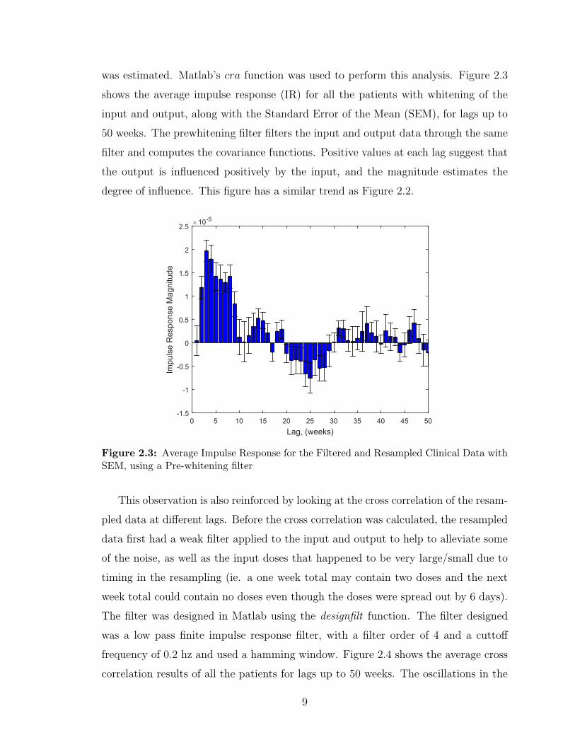
was estimated. Matlab’s cra function was used to perform this analysis. Figure 2.3
shows the average impulse response (IR) for all the patients with whitening of the
input and output, along with the Standard Error of the Mean (SEM), for lags up to
50 weeks. The prewhitening filter filters the input and output data through the same
filter and computes the covariance functions. Positive values at each lag suggest that
the output is influenced positively by the input, and the magnitude estimates the
degree of influence. This figure has a similar trend as Figure 2.2.
Lag, (weeks)0 5 10 15 20 25 30 35 40 45 50
Impu
lse
Res
pons
e M
agni
tude
×10-5
-1.5
-1
-0.5
0
0.5
1
1.5
2
2.5
Figure 2.3: Average Impulse Response for the Filtered and Resampled Clinical Data withSEM, using a Pre-whitening filter
This observation is also reinforced by looking at the cross correlation of the resam-
pled data at different lags. Before the cross correlation was calculated, the resampled
data first had a weak filter applied to the input and output to help to alleviate some
of the noise, as well as the input doses that happened to be very large/small due to
timing in the resampling (ie. a one week total may contain two doses and the next
week total could contain no doses even though the doses were spread out by 6 days).
The filter was designed in Matlab using the designfilt function. The filter designed
was a low pass finite impulse response filter, with a filter order of 4 and a cuttoff
frequency of 0.2 hz and used a hamming window. Figure 2.4 shows the average cross
correlation results of all the patients for lags up to 50 weeks. The oscillations in the
9
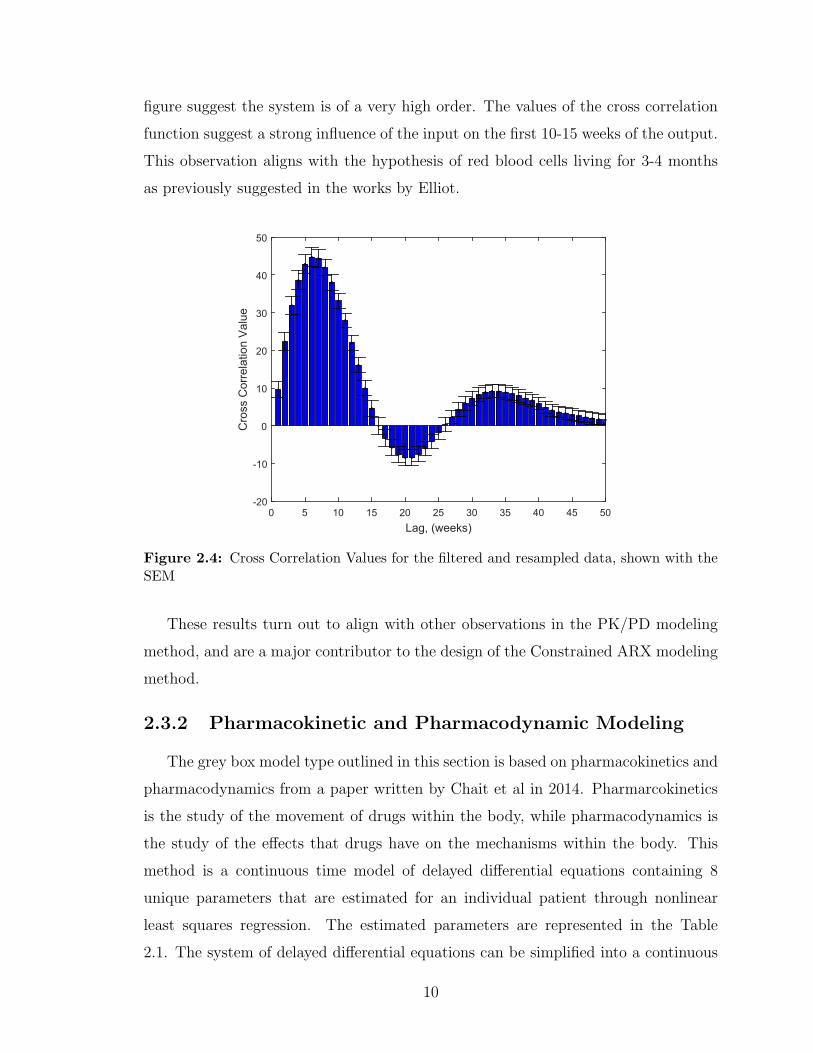
figure suggest the system is of a very high order. The values of the cross correlation
function suggest a strong influence of the input on the first 10-15 weeks of the output.
This observation aligns with the hypothesis of red blood cells living for 3-4 months
as previously suggested in the works by Elliot.
Lag, (weeks)0 5 10 15 20 25 30 35 40 45 50
Cro
ss C
orre
latio
n V
alue
-20
-10
0
10
20
30
40
50
Figure 2.4: Cross Correlation Values for the filtered and resampled data, shown with theSEM
These results turn out to align with other observations in the PK/PD modeling
method, and are a major contributor to the design of the Constrained ARX modeling
method.
2.3.2 Pharmacokinetic and Pharmacodynamic Modeling
The grey box model type outlined in this section is based on pharmacokinetics and
pharmacodynamics from a paper written by Chait et al in 2014. Pharmarcokinetics
is the study of the movement of drugs within the body, while pharmacodynamics is
the study of the effects that drugs have on the mechanisms within the body. This
method is a continuous time model of delayed differential equations containing 8
unique parameters that are estimated for an individual patient through nonlinear
least squares regression. The estimated parameters are represented in the Table
2.1. The system of delayed differential equations can be simplified into a continuous
10

Parameter Description
Hen Hemoglobin Level due to Endogenous Erythropoietinµ Mean RBC life spanV Maximal clearance rateKm Exogenous Erythropoietin level that produces half maximal clearance rateα Linear clearance constantS Maximal RBC production rate stimulated by EPC Amount of EP that produces half maximal RBC production rateD Time required for EPO-stimulated RBCs to start forming
Table 2.1: Estimated parameters and descriptions for the PK/PD Model
delayed nonlinear state space represented in Equation 2.2
Een =CHen
µ KH S −Hen
(2.2a)
dE(t)
dt=−V E(t)
Km + E(t)− α E(t) + dose(t) (2.2b)
dR(t)
dt=
S (Een + E(t−D))
(C + Een + E(t−D))− 4
x1(t)
µ2(2.2c)
dx1(t)
dt= x2(t) (2.2d)
dx2(t)
dt=
S (Een + E(t−D))
(C + Een + E(t−D))− 4
x1(t)
µ2− 4
x2(t)
µ(2.2e)
where the states E(t), R(t) represent the pool of exogenous erythropoietin and
the population of RBCs within the body. Ep is the summation of the endogenous
and exogenous erythropoietin. KH is the average amount of hemoglobin per RBC
(also known as the mean corpuscular hemoglobin, MCH). The value used here is
fixed at 29.5 pg/cell, which is within the reference range of 27-33 pg/cell (Chait et
al., 2014). The hemoglobin value is directly proportionate to the RBC population;
the hemoglobin value can be attained by multiplying the RBC population estimate by
the MCH value. The function dose(t) is a train of impulses, representing the EPO in-
jections, which are estimated to occur on the exact day they were administered. The
model has an initial condition as represented in Equations 2.3 and requires two mea-
surements of hemoglobin (hgb1 & hgb2) and the time in between those measurements
11

(t1 & t2) to estimate.
R0 =(hgb2 − hgb1)
KH(t2 − t1)(2.3a)
E(0) = 0 (2.3b)
R(0) =hgb1
KH
(2.3c)
x1(0) =µ(Hen − µ KH R0)
4KH
(2.3d)
x2(0) = R(0) − 4 x1(0)
µ(2.3e)
It should be relatively obvious, the difficulties this model structure presents in
estimating the model parameters by numerical computation methods. Firstly, the
model includes the impulse function in the first state’s derivative, dE(t)dt
, which intro-
duces some discontinuities into the solution. Secondly, the model includes a delayed
term, E(t − D), in two of the state equations. This presents a very difficult prob-
lem because the state, E(t), contains discontinuities and the delayed term allows the
discontinuities to propagate throughout the system (Christopher, 2000). In order to
effectively simulate this system, the discontinuities must be tracked and dealt with
appropriately by the careful selection of the step size. Thirdly, unless the step size
of the algorithm is fixed, the value for the delayed solution that is necessary for the
current estimate of the derivatives may not be available. An estimate for the past
solution must be used based on some sort of interpolation of the solution history.
These problems invite a short segue into the design of an efficient solver to estimate
these models.
Delayed Differential Equation Solver Design
As mentioned previously, it is desired to develop an efficient algorithm to simulate
the system mentioned in Equations 2.2 and 2.3. It would be easy to use a fixed
step size, first or second order method developed for ODEs and modify it to use the
delayed terms. This certainly works, but is incredibly inefficient. The desire here, is to
create an efficient solver, which naturally leads to a variable step size solver. Variable
step solvers are capable of modifying their step size, and producing some minimum
amount of taylor series truncation error when solving each point. The idea behind
12

variable step solvers is that they estimate each point using two different methods,
such as a first and second order Euler method, and then estimate the truncation
error from the difference in the solutions between the two methods. The algorithm
will check to make sure the error is within the desired user set tolerance. If it is
acceptable, the highest order value (usually the most accurate) is kept and the step
size is adjusted larger for the next iteration. If the point fails the error tolerances,
the step size is reduced and the iteration is re-run. Larger step sizes allow the solver
to skip over many calculations and the step size is desired to be as large as possible
without compromising the accuracy of the solution. Efficiency is also lost within the
solver for every failed iteration, so it is important to make appropriate adjustments
to the step size.
The algorithm that was chosen here was a modified version of the explicit Bogacki-
Shampine (2,3) variable step size algorithm (Bogacki and Shampine, 1989) for ODEs
which uses both a second order and a third order solution to estimate the truncation
error and adjust the step size. The local error estimate achieved is for the lower order
solution. The integration is advanced with the higher order solution because it is
believed to be more accurate (Shampine, 2004). Four coefficients must be estimated
using the current step size and second and third order estimates for the solution are
then given by Equations 2.4
k1 = f(tn, yn) (2.4a)
k2 = (tn +h
2, yn +
h k1
2) (2.4b)
k3 = f(tn +3 h
4, yn +
3 h k1
4) (2.4c)
yn+1 = yn +2 h k1
9+h k2
3+
4 h k3
9(2.4d)
k4 = f(tn + h, yn+1) (2.4e)
zn+1 = yn +7 h k1
24+h k2
4+h k3
3+h k4
8(2.4f)
where yn+1 represents the third order solution, and zn+1 represents the second order
solution. It should be noted that k4 for one iteration is the same estimate used for
k1 of the next iteration. This is a First Same As Last (FSAL) algorithm designed to
13
aid in reducing the computational burden. The local error estimate is computed by
Eest = Elocal + h.o.t. where h.o.t. are the higher order taylor expansion terms. The
error estimate must satisfy the following equation.
||Eest|| ≤ Rtol (2.5)
where Rtol is the relative error tolerance set by the user, and ||Eest|| is a suitable
weighted norm (Shampine, 2004). For this algorithm, we achieve an estimate for
||Eest|| by using Equation 2.6 (Shampine and Thompson, 2001).
||Eest|| = h ∗ ||[k1 k2 k3 k4][−5
72112
19−18
]T
max(|yn+1| , AtolRtol
)||∞ (2.6)
where Atol is the absolute error tolerance. If the error estimate is lower than the
relative tolerance, the iteration is successful and the step size is adjusted by one of
two ways. If the following equation is satisfied
1.25 ∗ (Eest/Rtol)13 > 0.2 (2.7)
then the new step size, hn+1 will be
hn+1 =hn
1.25 ∗ (Eest/Rtol)13
(2.8)
If Equation 2.7 is not satisfied, then
hn+1 = 5 ∗ hn (2.9)
One of the requirements of the algorithm is that the solution, yn+1, to the problem,
must be smooth. It is necessary to carefully choose the step sizes so that discontinu-
ities become mesh points, which will allow the algorithm to compute the proper esti-
mates for the solutions and the local error estimate (Shampine and Thompson, 2001).
To accomplish this, the discontinuities along with their propagations are tracked and
the step size is appropriately adjusted. For example, take the system delay, D, to be
7 days. If the patient is given a dose on day 8, their will be a discontinuity in the
derivative and solution for the first state, E(t), on day 8. The history of E(t) is used
in the second (R(t)) and fourth state (x1(t)) which means that on day 15, these states
and derivatives will cross the day 8 discontinuity in E(t) and create a discontinuity
14

in the solutions for these states. A discontinuity will propagate through the solution
D days after every dose. The location of these discontinuities are known and this
solver pre-calculates them before the integration starts. If the step size is to step over
a discontinuity, the step size is adjusted to be equal to the distance to the next dis-
continuity. The next point evaluated is immediately to the right of the discontinuity.
An example of a simulation using the DDE solver for one of the attained models is
shown in Figure 2.5.
0 5 10 15 20 25 30 35 40 45 50
E(t)
05000
1000015000
0 5 10 15 20 25 30 35 40 45 50
R(t)
0.3
0.4
0.5
0 5 10 15 20 25 30 35 40 45 50
x 1(t)
0
5
10
Time, t (days)0 5 10 15 20 25 30 35 40 45 50
x 2(t)
00.10.2
Figure 2.5: Example of the State Evolution when simulated with the designed DDE Solver
ARX Approximations of PK/PD Model
The nonlinear state space presented is difficult and slow to use within an MPC
routine. A nonlinear model predictive controller could certainly be built using func-
tions such as fmincon or IPOPT and will be introduced in the next chapter. The
nonlinear controller does present a few challenges though. Firstly, the DDE solver is
highly sensitive to inaccuracies in the initial condition, and there does not exist an
accurate way of calculating the initial derivative R0 needed for the initial condition.
Secondly, there are no guarantees that the DDE solver described above finds the
proper solution. Due to the fact that the numerical method is an explicit method,
the solver still runs a risk of becoming unstable which will greatly impact the opti-
mization problem within the MPC controller. In the design of an MPC controller,
the prediction horizon has been chosen to be 8 weeks. To start the DDE solver, it
15

requires a history of the solution up to D days previous to the solution to become the
most accurate. This is never available. For the first D days of the simulation, E(t) is
considered to be constant at zero, due to the lack of history data. This assumption
does not impact the model training algorithm significantly, but can certainly affect
the controller optimization problem over such a short prediction horizon.
It is desired to obtain a more convenient model, to avoid some of these problems.
One proposed approach is to design a random binary sequence (RBS) based on a
step test of the nonlinear model, and then subsequently filter it through the non-
linear model and use the resulting simulated data to obtain an ARX model. This
method was used for its simplicity, but also for exploring the structure of the ARX
models obtained, to aid in the design of the Constrained ARX method. Due to the
small control zone and minimal nonlinearities, the linearization of the models in this
manner does not introduce significant error. An example of an infinite step ahead
prediction comparison is shown in Figure 2.6. The fit of the PK/PD nonlinear model
is shown along with the ARX approximation and the actual data. It can be seen that
the ARX model provides a relatively good estimate of the nonlinear model as long
as the hemoglobin remains relatively close to the control zone. From looking at the
past patient history, it can be seen that the hemoglobin of the patients rarely exits a
zone of 8-13 g/dL.
Time, t (weeks)30 40 50 60 70 80 90 100 110 120 130
Hgb
, y (g
/dL)
7
8
9
10
11
12
13
14
15
ARX ApproximationActualNonlinear State Space
Figure 2.6: Example of the ARX approximation for the Nonlinear state space for aninfinite step ahead prediction
16

An example of the structure of the bk parameters is shown in Figure 2.7 for a
patient. Here the ARX model has an order of [1 13 2]. The system is described by
the following Equation.
Hgbt+1 −Hgbss =− a1 (Hgbt −Hgbss) . . .
+13∑k=1
bk (EPOt−k+1 − EPOss) + et(2.10)
Delay of Parameter (ie. u(k-d))1 2 3 4 5 6 7 8 9 10 11 12 13 14
Val
ue o
f Est
imat
ed b
k Par
amet
er
×10-5
-1
0
1
2
3
4
5
6
Figure 2.7: Example of the bk parameter structure for the PK/PD ARX approximation
After analyzing the obtained models, it was found that every identified ARX model
contained this same structure. That is, they all contained larger peak parameters at
the delay of two weeks, and then slowly decreased towards zero, usually in some
exponential decaying pattern. The majority of all the models contained only positive
bk parameters.
Using the PKPD-ARX models and matlabs deconv function, the impulse response
(IR) of a model can be estimated. deconv works by performing long division of the
B(z−1) polynomial by the A(z−1) polynomial, converting the ARX model directly to
an impulse response model. The IR models can be represented by equation
yt+1 =∞∑k=1
bkut−k+1 (2.11)
17

Figure 2.8 shows the average values for the coefficients in the IR models for all the
patients. Again, it can be seen that there exists a greater dependence on the models
on the first few weeks of past inputs, and the effect decays exponentially overtime.
Delay of Parameter (ie. u(k-d))0 5 10 15 20 25 30 35 40 45 50
Val
ue o
f Est
imat
ed b
k Par
amet
er
×10-5
0
0.5
1
1.5
2
2.5
3
3.5
4
4.5
Figure 2.8: Average values of the bk parameters in the IR models of all the estimatedPKPD-ARX models over 50 lags
A combination of the observations in the ARX models and the PK/PD mod-
els, along with the medical background knowledge, aided in the development of the
Constrained ARX modeling method which will be introduced next.
2.3.3 Constrained Autoregressive with Exogenous Inputs (C-ARX) Modeling
Inspired in part by the previous observations, a method of Constrained ARX
modeling was designed as outlined in detail in a conference paper written by Dr. Jia
Ren (Ren et al., 2017). This method again uses the re-sampled one week data. The
basic premise of the design is that the structure of the model is similar to the ARX
model mentioned earlier, but has the bk parameters constrained to be similar to the
ARX models identified from the PKPD models. The resulting model takes a similar
form as the PKPD-ARX, but it is much less restrictive on the location of the peak bk
parameter. The peak time parameter is allowed to float from a delay of 2 to a delay
18
of 4. Another major benefit of this design is that the hemoglobin and EPO value that
is used as the pseudo-steady state of the system is not the average value of the data,
but rather it is also optimized within the problem. This results in an extra 2 degrees
of freedom in the estimation problem.
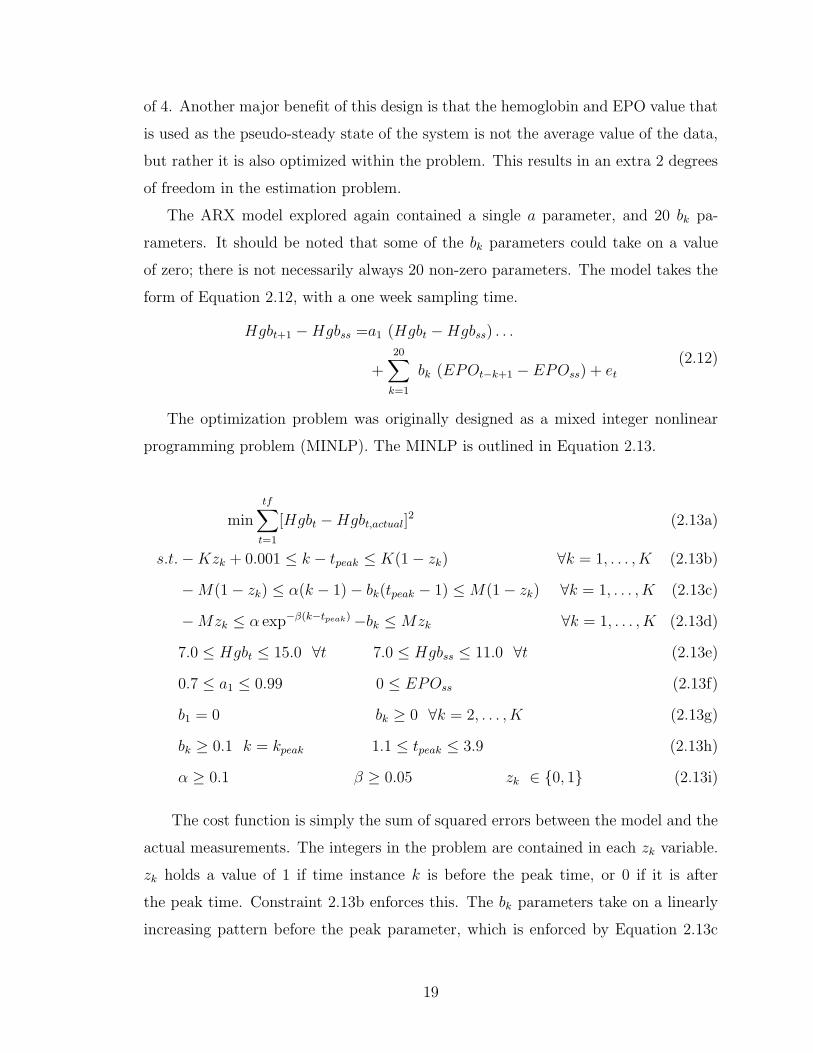
The ARX model explored again contained a single a parameter, and 20 bk pa-
rameters. It should be noted that some of the bk parameters could take on a value
of zero; there is not necessarily always 20 non-zero parameters. The model takes the
form of Equation 2.12, with a one week sampling time.
Hgbt+1 −Hgbss =a1 (Hgbt −Hgbss) . . .
+20∑k=1
bk (EPOt−k+1 − EPOss) + et(2.12)
The optimization problem was originally designed as a mixed integer nonlinear
programming problem (MINLP). The MINLP is outlined in Equation 2.13.
min
tf∑t=1
[Hgbt −Hgbt,actual]2 (2.13a)
s.t.−Kzk + 0.001 ≤ k − tpeak ≤ K(1− zk) ∀k = 1, . . . , K (2.13b)
−M(1− zk) ≤ α(k − 1)− bk(tpeak − 1) ≤M(1− zk) ∀k = 1, . . . , K (2.13c)
−Mzk ≤ α exp−β(k−tpeak)−bk ≤Mzk ∀k = 1, . . . , K (2.13d)
7.0 ≤ Hgbt ≤ 15.0 ∀t 7.0 ≤ Hgbss ≤ 11.0 ∀t (2.13e)
0.7 ≤ a1 ≤ 0.99 0 ≤ EPOss (2.13f)
b1 = 0 bk ≥ 0 ∀k = 2, . . . , K (2.13g)
bk ≥ 0.1 k = kpeak 1.1 ≤ tpeak ≤ 3.9 (2.13h)
α ≥ 0.1 β ≥ 0.05 zk ∈ {0, 1} (2.13i)
The cost function is simply the sum of squared errors between the model and the
actual measurements. The integers in the problem are contained in each zk variable.
zk holds a value of 1 if time instance k is before the peak time, or 0 if it is after
the peak time. Constraint 2.13b enforces this. The bk parameters take on a linearly
increasing pattern before the peak parameter, which is enforced by Equation 2.13c
19

and the variable α.
bk =α(k − 1)
tpeak − 1(2.14)
It should be noted that tpeak is a continuous variable, meaning the peak time can exist
anywhere from 1.1 to 3.9 and α is the value of the parameter at that peak time. The
bk parameters take on an exponentially decreasing pattern after the peak parameter,
which is enforced by Equation 2.13d, and the variable β, which is the decay rate.
Equation 2.13d reduces to the following Equation for bk parameters after the peak
time.
bk = α exp−β(k−tpeak) (2.15)
Equations 2.13e,f help to enforce physically realizable solutions. The constraints on
a1 ensure the resulting model is open-loop stable. Another important equation is
Equation 1 of line 2.13h. It is important to constrain the first bk parameter after the
peak time parameter for kpeak to be above 0.1. This ensures the model reliance on
the past doses and overcomes the issues arising from the small gain of the inputs as
mentioned in Section 2.3.1.
MINLP problems are relatively difficult to solve. There are commercially available
solvers such as DICOPT in GAMS mentioned in the paper that are capable of finding
this solution, efficiently. To reduce the computational complexity, the MINLP was
converted to a series of nonlinear programming (NLP) problems. That is, instead of
solving the integer variables for zk in the optimization problem, the values are fixed
at a specific value and then an NLP problem can be solved. This can be performed
for all the combinations of zk because there are only 3 different combinations that can
occur for the chosen constraint on tpeak. The constraint bk ≥ 0.1 for k = kpeak will
also have to be modified for each case. The values of the cost functions are compared,
and the model corresponding to the lowest cost function solution will be chosen as the
best model. This iterative NLP problem is solved using both an IPOPT interface for
Matlab as well as Matlab’s native fmincon function. It is desired to have a complete
Matlab solution for on-line implementation. It has been recognized that IPOPT is
more robust than fmincon in some situations, and this will be explored in the next
section.
Using the C-ARX models and Matlab’s deconv function, the IR of a model can be
20

estimated. Figure 2.9 shows the average values for the coefficients in the IR models
for all the patients. The IRs again take on a similar shape as the cross correlation
function figure and the IR of the PKPD-ARX models.
Delay of Parameter (ie. u(k-d))0 5 10 15 20 25 30 35 40 45 50
Val
ue o
f Est
imat
ed b
k Par
amet
er
0
0.02
0.04
0.06
0.08
0.1
0.12
0.14
Figure 2.9: Average values of the bk parameters in the IR models of all the estimatedC-ARX models over 50 lags
2.3.4 Linear C-ARX Modeling
A conversion of the original nonlinear C-ARX modeling method was also explored.
In the next Chapter, recursive modeling will be introduced for a control algorithm,
where a new model is obtained after each new updated hemoglobin measurement.
This requires a robust modeling method, which naturally leads to a conversion of the
nonlinear problem to a linear problem. The only nonlinearities in the method are
built into the shape of the bk parameters and the steady state values. The steady
state values can be taken as the average Hgb and EPO dose from the data used for the
model estimation. The bk parameter shape can be replaced by making each successive
bk parameter a certain percentage lower/higher depending on whether the parameter
is before or after the peak time parameter. The model order was also reduced to a
[1 8 1] ARX model. Three optimization problems are still solved for each peak time
location, and again the best solution can be chosen. With this alteration, the problem
21
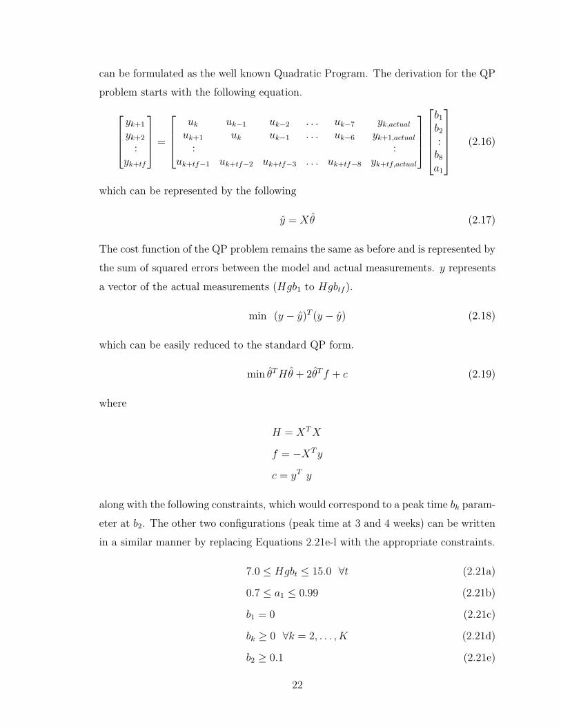
can be formulated as the well known Quadratic Program. The derivation for the QP
problem starts with the following equation.
yk+1
yk+2
:yk+tf
=
uk uk−1 uk−2 . . . uk−7 yk,actualuk+1 uk uk−1 . . . uk−6 yk+1,actual
: :uk+tf−1 uk+tf−2 uk+tf−3 . . . uk+tf−8 yk+tf,actual
b1
b2
:b8
a1
(2.16)
which can be represented by the following
y = Xθ (2.17)
The cost function of the QP problem remains the same as before and is represented by
the sum of squared errors between the model and actual measurements. y represents
a vector of the actual measurements (Hgb1 to Hgbtf ).
min (y − y)T (y − y) (2.18)
which can be easily reduced to the standard QP form.
min θTHθ + 2θTf + c (2.19)
where
H = XTX
f = −XTy
c = yT y
along with the following constraints, which would correspond to a peak time bk param-
eter at b2. The other two configurations (peak time at 3 and 4 weeks) can be written
in a similar manner by replacing Equations 2.21e-l with the appropriate constraints.
7.0 ≤ Hgbt ≤ 15.0 ∀t (2.21a)
0.7 ≤ a1 ≤ 0.99 (2.21b)
b1 = 0 (2.21c)
bk ≥ 0 ∀k = 2, . . . , K (2.21d)
b2 ≥ 0.1 (2.21e)
22
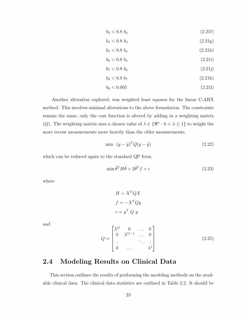
b3 < 0.8 b2 (2.21f)
b4 < 0.8 b3 (2.21g)
b5 < 0.8 b4 (2.21h)
b6 < 0.8 b5 (2.21i)
b7 < 0.8 b6 (2.21j)
b8 < 0.8 b7 (2.21k)
b8 < 0.005 (2.21l)
Another alteration explored, was weighted least squares for the linear C-ARX
method. This involves minimal alterations to the above formulation. The constraints
remain the same, only the cost function is altered by adding in a weighting matrix
(Q). The weighting matrix uses a chosen value of λ ∈ {<n : 0 < λ ≤ 1} to weight the
more recent measurements more heavily than the older measurements.
min (y − y)TQ(y − y) (2.22)
which can be reduced again to the standard QP form.
min θTHθ + 2θTf + c (2.23)
where
H = XTQX
f = −XTQy
c = yT Q y
and
Q =
λtf 0 . . . 00 λtf−1 . . . 0
:. . . :
0 . . . λ1
(2.25)
2.4 Modeling Results on Clinical Data
This section outlines the results of performing the modeling methods on the avail-
able clinical data. The clinical data statistics are outlined in Table 2.2. It should be
23

noted that there was no pre-screening of patients completed before attempting the
modeling methods. For instance, there exists some patients that have no dose for the
first half of the data. It is well known, this cannot possibly lead to a proper model.
Similar situations exist for some other patients that may cause some of the modeling
methods to fail. The cases where the modeling method fails will be filtered out after
all models are obtained and tested. The filtration method will be discussed later in
this section. The first 50% of the data was used as training data sets, and the models
were validated on the last 50% of the data. The figures shown in this section start
from the first actual hgb measurement that occurs at a time just after the initial
condition. Due to the number of bk coefficients, the simulation data for the training
set do not start until 21 weeks after the initial point. Also, as the sampling time does
not fall directly on these measurement days, a linear interpolation was used between
the closest points for each modeling type. For the validation portion of the data, the
simulation was reset to an initial condition matching the first actual hgb data point
in that data range.
Statistic ValueNumber of Patients 168Hemoglobin (Mean ± std ) 10.48 ±0.57EPO dose, IU/week (Mean ± std ) 3167.2 ± 2484.4Hgb Measurement Frequency (approximate) 2 weeksAverage Patient Data Length (Mean ± std ) 126.4 ±19.7 (weeks)
Table 2.2: Statistics describing the clinical data used in the modeling methods
The results of the different modeling types on the clinical data are shown in Table
2.3. The results for the C-ARX are done using three different optimization solvers.
The MINLP problem is solved directly in GAMS using DICOPTS. The NLP problem
is solved using fmincon and also against a third party matlab interface for IPOPT.
A couple initial conclusions can be made from these unfiltered results. It can be seen
that the ARX modeling method (all types) tend to model more of the system noise.
This can be inferred by the fact that the mean training RMSE is much better than
the PKPD modeling method, yet the mean validation RMSE is significantly larger
proportionally when compared to that of the PKPD modeling method. An example
of this is shown in Figure 2.10. The NLP model in the figure represents the solution
24

obtained from Matlab’s fmincon.
Mean RMSE Std RMSE ModelsModeling Method Training Validation Training Validation Included
Classical ARX 1.12 5.06 3.24 21.18 168Constrained ARX - MINLP 0.70 1.87 0.33 5.14 158Constrained ARX - NLP (fmincon) 0.76 1.66 0.50 1.42 168Constrained ARX - NLP (IPOPT) 0.76 1.66 0.50 1.43 168PKPD 0.94 1.61 0.68 2.59 167PKPD-ARX Approximations 1.47 2.72 3.54 11.26 158
Table 2.3: Modeling Results of the unfiltered models for the various modeling methodsexplored along with the number of models included in the resulting statistics
100 200 300 400 500 600 700 800 900 1000
Hgb
, (g/
dL)
7
8
9
10
11
12
13
14
15
NLPMINLPPKPDARXActual
Time, (days)100 200 300 400 500 600 700 800 900 1000
EP
O, (
IU) ×104
0
5
10
Figure 2.10: Example that shows the ARX modeling methods capturing the peaks of thedata, where as the PKPD model does not capture the sharpness of the data peaks
The validation statistics for the Classical ARX method are very poor. From the
filtered results, it will be shown that there are a few patients that skew these statistics
greatly. This phenomenon is a result of an ill-conditioned X matrix in some of the
patients when estimating the parameter set, θ, using the formula θ = (XTX)−1XTY .
25

This situation occurs when two rows or columns of the matrix X are the same or
similar. Mathematically, this means the regressors are colinear or close to colinear
(Soderstrom and Stoica, 1989). An example of this can be seen in Figure 2.11.
100 200 300 400 500 600 700 800 900 1000
Hgb
, (g/
dL)
7
8
9
10
11
12
13
14
15
NLPMINLPPKPDARXActual
Time, (days)100 200 300 400 500 600 700 800 900 1000
EP
O, (
IU)
0
5000
10000
Figure 2.11: ARX modeling Algorithm fails to estimate a proper model. Modeling resultsfor both training and validation data for all modeling methods
Another thing that can be seen in this data, is that both the NLP versions of
the constrained ARX modeling using IPOPT and fmincon result in almost identical
statistics. Due to the extra complexity, it is not worth using IPOPT over fmincon in
a practical application, as it does not offer a substantial benefit.
Table 2.4 shows the filtered modeling results. Firstly, the filtered results confirm
the fact that some patients skew the results in the Classical ARX modeling. The
results are as expected for Classical ARX modeling because the training error is very
close to the C-ARX modeling methods. The C-ARX method has two extra degrees
of freedom allowing it have lower training error on some patients, even with the
modeling structure constrained. Both the C-ARX methods using the MINLP and
26

the NLP problem yield very similar results. On average, these results show that the
C-ARX modeling method works better than Classical ARX and the PKPD modeling
methods. The C-ARX is certainly better than Classical ARX as it provides lower
validation RMSE on a larger number of models than the Classical ARX method.
As will be discussed later, it is not overly desired to have a nonlinear modeling
method for control purposes. On average, the C-ARX provides better results than the
PKPD modeling method with the added benefit that the C-ARX models are linear,
and estimated more easily and efficiently in Matlab. The algorithm for converting
the PKPD models to PKPD-ARX approximations is based on performing successive
step tests on the attained models using a bisection optimization algorithm to find
corresponding EPO levels of the system that center the step test around the control
zone of 9.5-11.0 g/dL. Using these results, an RBS was designed and the models can
be converted to linear ARX models. It can be seen that the algorithm in its present
form fails to identify a good linear model for some of the patients, which may be a
result of the PKPD modeling method not achieving a proper model in the first place,
or a failure in the conversion algorithm. When some of the worse models are filtered
out of the PKPD-ARX models, it can be seen that these approximations result in
relatively close performance to their nonlinear counterparts.
Mean RMSE Std RMSE ModelsModeling Method Training Validation Training Validation Included
Classical ARX 0.70 1.28 0.62 0.66 136Constrained ARX - MINLP 0.70 1.21 0.34 0.58 145Constrained ARX - NLP (fmincon) 0.69 1.18 0.35 0.60 144PKPD 0.83 1.23 0.37 0.62 153PKPD-ARX Approximations 1.09 1.26 0.62 0.60 133
Table 2.4: Modeling Results for the various modeling methods where patients with vali-dation RMSE ≥ 3 removed from corresponding model type
Figure 2.13 shows the modeling techniques exhibit a degree of robustness against
acute step disturbances, such as infections or blood losses. These scenarios present
difficulty in determining dosing and how the patient’s hemoglobin will respond to the
ESA treatment.
27

100 200 300 400 500 600 700 800 900 1000
Hgb
, (g/
dL)
7
8
9
10
11
12
13
14
15
NLPMINLPPKPDARXActual
Time, (days)100 200 300 400 500 600 700 800 900 1000
EP
O, (
IU) ×104
0
1
2
Figure 2.12: Example patient showing the modeling methods robustness for rejectingdisturbances in the training data
Figure 2.12 shows an example where the patient model significantly changes over
the course of the patients history. The patient’s health deteriorates and the patient
continually needs a higher degree of ESAs to manage their anemia. All modeling
types validate poorly on this patient. As all patients will generally become more sick
over time, this brings about the need to recursively attain new models for each patient
to be able to capture the time-varying nature of the model parameters. Recursive
modeling results will be obtained for the clinical data and presented later in this
chapter.
28

100 200 300 400 500 600 700 800 900 1000
Hgb
, (g/
dL)
7
8
9
10
11
12
13
14
15NLPMINLPPKPDARXActual
Time, (days)100 200 300 400 500 600 700 800 900 1000
EP
O, (
IU) ×104
0
1
2
Figure 2.13: Example of a patient where the health continually deteriorates over thelength of the patient history.
2.4.1 Model Order Reduction
It is desired to reduce the model order of the [1 20 1] nonlinear C-ARX models. A
reduction in model order should yield a positive impact on the model estimation due
to the fact that, in practice, more data points are available to perform the estimation.
Another reason it should offer improvements, is that a large number of parameters
often result in the modeling of noise in the system, which is undesirable. To perform
the system identification with the new model orders, the same number of data points
were used in each case, even though there would be extra data points for the C-ARX
models with lower orders. This was done to be able to more accurately compare
the model orders. Another small change from the original C-ARX conference paper
is the addition of a constraint on the final bk parameter. This was done to avoid
large system gains seen in models that have low training RMSE values, but poor
29
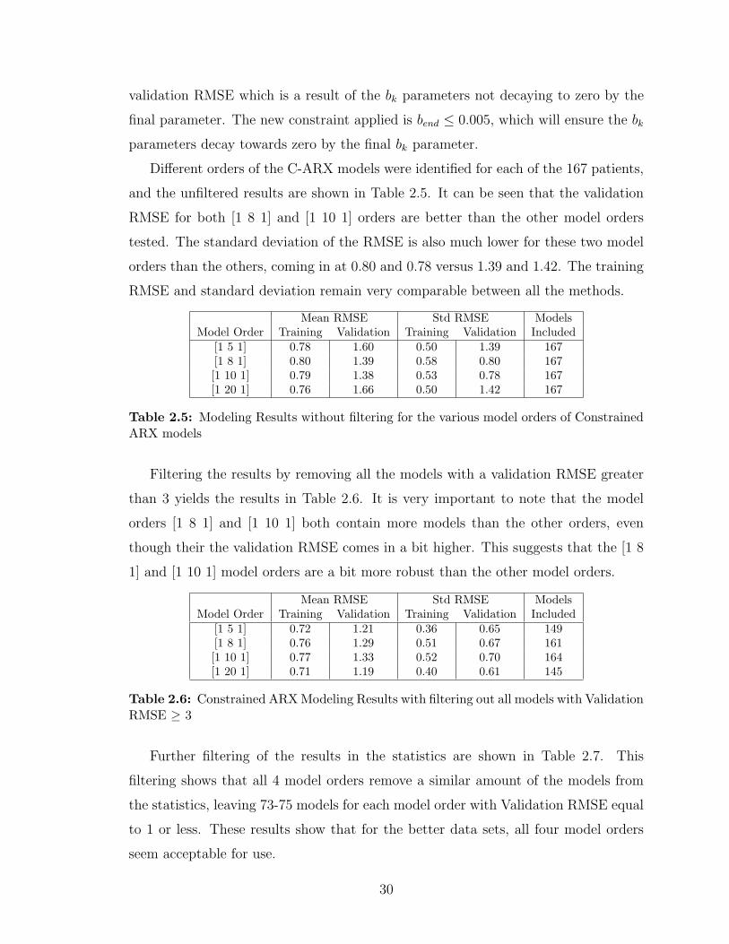
validation RMSE which is a result of the bk parameters not decaying to zero by the
final parameter. The new constraint applied is bend ≤ 0.005, which will ensure the bk
parameters decay towards zero by the final bk parameter.
Different orders of the C-ARX models were identified for each of the 167 patients,
and the unfiltered results are shown in Table 2.5. It can be seen that the validation
RMSE for both [1 8 1] and [1 10 1] orders are better than the other model orders
tested. The standard deviation of the RMSE is also much lower for these two model
orders than the others, coming in at 0.80 and 0.78 versus 1.39 and 1.42. The training
RMSE and standard deviation remain very comparable between all the methods.
Mean RMSE Std RMSE ModelsModel Order Training Validation Training Validation Included
[1 5 1] 0.78 1.60 0.50 1.39 167[1 8 1] 0.80 1.39 0.58 0.80 167[1 10 1] 0.79 1.38 0.53 0.78 167[1 20 1] 0.76 1.66 0.50 1.42 167
Table 2.5: Modeling Results without filtering for the various model orders of ConstrainedARX models
Filtering the results by removing all the models with a validation RMSE greater
than 3 yields the results in Table 2.6. It is very important to note that the model
orders [1 8 1] and [1 10 1] both contain more models than the other orders, even
though their the validation RMSE comes in a bit higher. This suggests that the [1 8
1] and [1 10 1] model orders are a bit more robust than the other model orders.
Mean RMSE Std RMSE ModelsModel Order Training Validation Training Validation Included
[1 5 1] 0.72 1.21 0.36 0.65 149[1 8 1] 0.76 1.29 0.51 0.67 161[1 10 1] 0.77 1.33 0.52 0.70 164[1 20 1] 0.71 1.19 0.40 0.61 145
Table 2.6: Constrained ARX Modeling Results with filtering out all models with ValidationRMSE ≥ 3
Further filtering of the results in the statistics are shown in Table 2.7. This
filtering shows that all 4 model orders remove a similar amount of the models from
the statistics, leaving 73-75 models for each model order with Validation RMSE equal
to 1 or less. These results show that for the better data sets, all four model orders
seem acceptable for use.
30
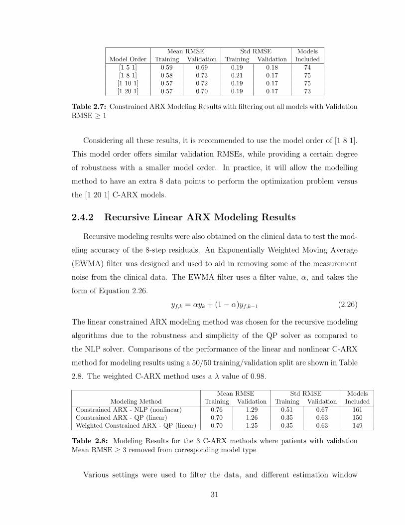
Mean RMSE Std RMSE ModelsModel Order Training Validation Training Validation Included
[1 5 1] 0.59 0.69 0.19 0.18 74[1 8 1] 0.58 0.73 0.21 0.17 75[1 10 1] 0.57 0.72 0.19 0.17 75[1 20 1] 0.57 0.70 0.19 0.17 73
Table 2.7: Constrained ARX Modeling Results with filtering out all models with ValidationRMSE ≥ 1
Considering all these results, it is recommended to use the model order of [1 8 1].
This model order offers similar validation RMSEs, while providing a certain degree
of robustness with a smaller model order. In practice, it will allow the modelling
method to have an extra 8 data points to perform the optimization problem versus
the [1 20 1] C-ARX models.
2.4.2 Recursive Linear ARX Modeling Results
Recursive modeling results were also obtained on the clinical data to test the mod-
eling accuracy of the 8-step residuals. An Exponentially Weighted Moving Average
(EWMA) filter was designed and used to aid in removing some of the measurement
noise from the clinical data. The EWMA filter uses a filter value, α, and takes the
form of Equation 2.26.
yf,k = αyk + (1− α)yf,k−1 (2.26)
The linear constrained ARX modeling method was chosen for the recursive modeling
algorithms due to the robustness and simplicity of the QP solver as compared to
the NLP solver. Comparisons of the performance of the linear and nonlinear C-ARX
method for modeling results using a 50/50 training/validation split are shown in Table
2.8. The weighted C-ARX method uses a λ value of 0.98.
Mean RMSE Std RMSE ModelsModeling Method Training Validation Training Validation Included
Constrained ARX - NLP (nonlinear) 0.76 1.29 0.51 0.67 161Constrained ARX - QP (linear) 0.70 1.26 0.35 0.63 150Weighted Constrained ARX - QP (linear) 0.70 1.25 0.35 0.63 149
Table 2.8: Modeling Results for the 3 C-ARX methods where patients with validationMean RMSE ≥ 3 removed from corresponding model type
Various settings were used to filter the data, and different estimation window
31

lengths were explored when comparing the 8-step residuals obtained from recursively
estimating a model at each sampling instant. The highlights of these results are
presented in Table 2.9. It should be noted that the accuracy of the 8-step predic-
tion is highly dependent on the initial condition, and the hemoglobin has very slow
dynamics. This means the measurement noise of the clinical data may significantly
effect the accuracy of the 8-step predictions. The highlights presented here show
that the modeling accuracy improves as the window estimation size increases. It also
shows a λ that is around 0.98 to 1.0 gives similar results, but a lower λ causes the
modeling accuracy to decay. A higher λ value puts more equal weighting on all the
measurements, where as a lower value puts much more weight on the newer measure-
ments. Due to the complexities of the NLP solver and the PKPD model estimation,
the linear versions of the C-ARX methods were selected to test the recursive con-
troller algorithms. An estimation window length of 70 gives good accuracy of the
hemoglobin predictions, but the linear C-ARX modeling method can be used on less
data. In a clinical setting, there may not exist more than a years worth of data, but
this shows the modeling method can be used with less data points, without too much
deterioration in model accuracy.
Model Method Non-Weighted Weighted Weighted Weighted Weighted
Training Window Size 70 30 50 70 70Weighting Value (λ) – 0.98 0.98 0.98 0.95
Mean -0.05 -0.08 -0.04 -0.06 -0.08Standard Deviation 1.04 1.26 1.20 1.05 1.09
Mean (absolute) 0.76 0.87 0.81 0.77 0.7890% Confidence Interval ± 1.71 ± 2.08 ± 1.97 ± 1.73 ± 1.80
Table 2.9: Highlights of the Recursive Modeling 8-Step Residual Statistics for the LinearC-ARX modeling methods with various settings
2.5 Conclusions
In this chapter, three different modeling methods were explored. The classical
ARX method was chosen as a base to compare the other models too. The classical
ARX models that were estimated were of order [1 20 1]. A DDE modeling method was
also used based on pharmacokinetics and pharmacodynamics. This method used a
fixed model structure and eight parameters within the model structure were estimated
by using an individual patients’ data along with nonlinear least squares regression in
32

Matlab. The third method used was the method of attaining a [1 20 1] order ARX
model through constrained optimization. In this modeling technique, the steady
state values were also optimized. The magnitudes of the parameters were constrained
to follow certain patterns learned from the first two methods. The three modeling
methods were tested on the clinical patient data and compared for all 167 patients.
It was found that on average the Constrained ARX models outperformed the other
modeling methods. The classical ARX modeling method performed the worst as was
expected due to the impact of large process and measurement noise in the clinical
data, along with a relatively large amount of b parameters. These ARX models
tended to over-fit the noise. The C-ARX modeling method performed quite similar
to the DDE modeling method, but has the benefit of being linear, and efficiently
estimated.
Model order reduction for the Constrained ARX models was also explored. It was
found that reducing the model order to [1 8 1] resulted in a good balance between
robustness and model accuracy. It resulted in comparable RMSE values to the [1
20 1] models, but with less parameters to estimate. The [1 8 1] model order was
also shown to be more robust than the [1 5 1] model order. The [1 8 1] and [1 10 1]
results were extremely close in values and were both considered for the final suggested
model order. The final choice for the model order for the Constrained ARX modeling
method is of order [1 8 1] because there are less parameters to estimate than the [1
10 1]. For the purpose of controller design, the [1 8 1] Constrained ARX models offer
the best modeling solution.
A weighted and non-weighted linear version of the nonlinear C-ARX method was
also introduced. The results show that the linear version of the C-ARX modeling
methods yields similar results on the 50/50 training/validation tests as the nonlinear
method. The linear C-ARX uses a simple QP formulation. QP solvers are more robust
than NLP solvers are and are more desirable to use. Both the weighted and non-
weighted versions performed similar on the 50/50 modeling results. The two linear
methods were also selected to explore the effect of window size and weighting values
on the 8-step prediction residuals. The results from the recursive modeling results
suggested that a longer window and higher value of λ were better at predicting the hgb
8 weeks later. It should be noted that the accuracy of the 8-step predictions is highly
33

dependent on the initial condition, which can be greatly affected by measurement
noise. The data was filtered with an EWMA filter to try and remove some of the
effect of the noise. Taken altogether, it is recommended that either the weighted or
non-weighted linear C-ARX modeling method with an order of [1 8 1] should be used
within the controller. Both the linear and nonlinear methods will be explored further
in the controller performance tests.
34

Chapter 3
Hemoglobin Controller Designs
3.1 Introduction
Chapter 3 explores the development of several different types of model predictive
controllers to be used to dose epoetin-alfa in the control of hemoglobin in CKD. The
optimal hemoglobin target range is still up for debate (Singh, 2007) but generally lies
somewhere between 9.5 and 12.0 g/dL for CKD patients. The tremendous cost of
ESA therapy leaves a lot of room for debate on this issue, and there becomes a fine
line where one could sacrifice patient health for monetary gain. For the purpose of
this thesis, a control zone of 9.5 to 11.0 g/dL will be used. This range was chosen
based on the available physician’s protocol that the controllers will be compared to.
There exist a few problems with a one-size-fits-all protocol for delivering ESA’s to the
patients. First, many of these protocols make doses based on a patient’s weight, even
though this is poorly correlated, as is shown in Figure 3.1. Secondly, the protocols lack
the ability to counter acute disturbances in the hemoglobin in the patients, such as
infection, blood loss or blood transfusions. The protocol that is used for comparison in
this paper, is generally sluggish with its choice of ESA dosing and often fails to react
quickly when presented with acute disturbances. Frequent disturbances, along with
the reactive behaviour of the protocol, cause bouts of hemoglobin cycling. Thirdly,
due to the large delay in the system caused by the pharmacokinetics and the delay
in the production of red blood cells, it is extremely difficult to control by reactive
measures as the protocol will always be a week or two behind the system dynamics.
35
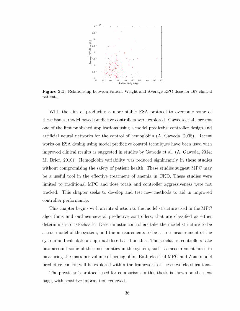
Patient Weight (kg)20 40 60 80 100 120 140 160 180 200
Ave
rage
EP
O D
ose
(IU)
×104
0
0.5
1
1.5
2
2.5
3
3.5
4
Figure 3.1: Relationship between Patient Weight and Average EPO dose for 167 clinicalpatients
With the aim of producing a more stable ESA protocol to overcome some of
these issues, model based predictive controllers were explored. Gaweda et al. present
one of the first published applications using a model predictive controller design and
artificial neural networks for the control of hemoglobin (A. Gaweda, 2008). Recent
works on ESA dosing using model predictive control techniques have been used with
improved clinical results as suggested in studies by Gaweda et al. (A. Gaweda, 2014;
M. Brier, 2010). Hemoglobin variability was reduced significantly in these studies
without compromising the safety of patient health. These studies suggest MPC may
be a useful tool in the effective treatment of anemia in CKD. These studies were
limited to traditional MPC and dose totals and controller aggressiveness were not
tracked. This chapter seeks to develop and test new methods to aid in improved
controller performance.
This chapter begins with an introduction to the model structure used in the MPC
algorithms and outlines several predictive controllers, that are classified as either
deterministic or stochastic. Deterministic controllers take the model structure to be
a true model of the system, and the measurements to be a true measurement of the
system and calculate an optimal dose based on this. The stochastic controllers take
into account some of the uncertainties in the system, such as measurement noise in
measuring the mass per volume of hemoglobin. Both classical MPC and Zone model
predictive control will be explored within the framework of these two classifications.
The physician’s protocol used for comparison in this thesis is shown on the next
page, with sensitive information removed.
36

Figure 3.2: Physician’s Protocol for dosing Epoetin-alfa
37
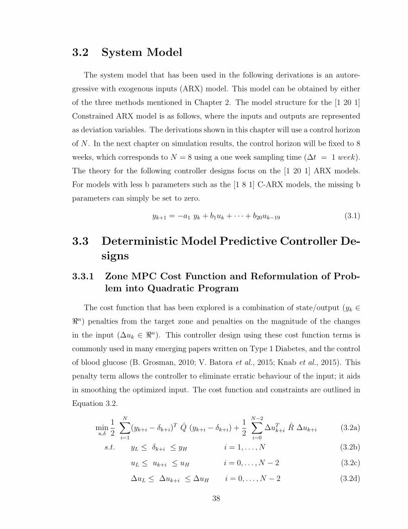
3.2 System Model
The system model that has been used in the following derivations is an autore-
gressive with exogenous inputs (ARX) model. This model can be obtained by either
of the three methods mentioned in Chapter 2. The model structure for the [1 20 1]
Constrained ARX model is as follows, where the inputs and outputs are represented
as deviation variables. The derivations shown in this chapter will use a control horizon
of N . In the next chapter on simulation results, the control horizon will be fixed to 8
weeks, which corresponds to N = 8 using a one week sampling time (∆t = 1 week).
The theory for the following controller designs focus on the [1 20 1] ARX models.
For models with less b parameters such as the [1 8 1] C-ARX models, the missing b
parameters can simply be set to zero.
yk+1 = −a1 yk + b1uk + · · ·+ b20uk−19 (3.1)
3.3 Deterministic Model Predictive Controller De-
signs
3.3.1 Zone MPC Cost Function and Reformulation of Prob-lem into Quadratic Program
The cost function that has been explored is a combination of state/output (yk ∈
<n) penalties from the target zone and penalties on the magnitude of the changes
in the input (∆uk ∈ <n). This controller design using these cost function terms is
commonly used in many emerging papers written on Type 1 Diabetes, and the control
of blood glucose (B. Grosman, 2010; V. Batora et al., 2015; Knab et al., 2015). This
penalty term allows the controller to eliminate erratic behaviour of the input; it aids
in smoothing the optimized input. The cost function and constraints are outlined in
Equation 3.2.
minu,δ
1
2
N∑i=1
(yk+i − δk+i)T Q (yk+i − δk+i) +
1
2
N−2∑i=0
∆uTk+i R ∆uk+i (3.2a)
s.t. yL ≤ δk+i ≤ yH i = 1, . . . , N (3.2b)
uL ≤ uk+i ≤ uH i = 0, . . . , N − 2 (3.2c)
∆uL ≤ ∆uk+i ≤ ∆uH i = 0, . . . , N − 2 (3.2d)
38
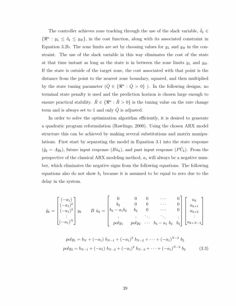
The controller achieves zone tracking through the use of the slack variable, δk ∈
{<n : yL ≤ δk ≤ yH}, in the cost function, along with its associated constraint in
Equation 3.2b. The zone limits are set by choosing values for yL and yH in the con-
straint. The use of the slack variable in this way eliminates the cost of the state
at that time instant as long as the state is in between the zone limits yL and yH .
If the state is outside of the target zone, the cost associated with that point is the
distance from the point to the nearest zone boundary, squared, and then multiplied
by the state tuning parameter (Q ∈ {<n : Q > 0} ). In the following designs, no
terminal state penalty is used and the prediction horizon is chosen large enough to
ensure practical stability. R ∈ {<n : R > 0} is the tuning value on the rate change
term and is always set to 1 and only Q is adjusted.
In order to solve the optimization algorithm efficiently, it is desired to generate
a quadratic program reformulation (Rawlings, 2000). Using the chosen ARX model
structure this can be achieved by making several substitutions and matrix manipu-
lations. First start by separating the model in Equation 3.1 into the state response
(yk = Ayk), future input response (Buk), and past input response (PUk). From the
perspective of the classical ARX modeling method, a1 will always be a negative num-
ber, which eliminates the negative signs from the following equations. The following
equations also do not show b1 because it is assumed to be equal to zero due to the
delay in the system.
yk =
(−a1)(−a1)2
(−a1)3
:(−a1)N
yk B uk =
0 0 0 · · · 0b2 0 0 · · · 0
b3 − a1b2 b2 0 · · · 0
: :. . . . . . :
poly1 poly2 · · · b3 − a1 b2 b2
ukuk+1
uk+2
:uk+N−2
poly1 = bN + (−a1) bN−1 + (−a1)2 bN−2 + · · ·+ (−a1)N−2 b2
poly2 = bN−1 + (−a1) bN−2 + (−a1)2 bN−3 + · · ·+ (−a1)N−3 b2 (3.3)
39

P Uk =
b2 b3 b4 · · · b20
(−a1) b2 + b3 b4 + (−a1) b3 · · · · · · (−a1) b20
(−a1)2 b2 + (−a1) b3 + b4 : · · · · · · (−a1)2 b20
: :. . . . . . :
poly3 poly4 · · · poly5 (−a1)N−1 b20
uk−1
uk−2
uk−3
:uk−19
poly3 = b2 (−a1)N−1 + b3 (−a1)N−2 + b4 (−a1)N−3 + b5 (−a1)N−4 + b6 (−a1)N−5 + . . .
poly4 = b3 (−a1)N−1 + b4 (−a1)N−2 + b5 (−a1)N−3 + b6 (−a1)N−4 + b7 (−a1)N−5 + . . .
poly5 = b19 (−a1)N−1 + b20 (−a1)N−2
The following matrices are also needed in the reformulation.
yk =
yk+1
yk+2
:yk+N
δk =
δk+1
δk+2
:δk+N
yL =
yL,k+1
yL,k+2
:yL,k+N
yH =
yH,k+1
yH,k+2
:yH,k+N
uk =
uk−1
0:0
uk =
ukuk+1
:uk+N−2
∆uk =
∆uk
∆uk+1
:∆uk+N−2
(3.4)
φ =
1 0 . . . 0−1 1 . . . 0
:. . . . . . 0
0 0 −1 1
Q =
Q 0 . . . 0
0 Q . . . 0
: :. . . :
0 0 . . . Q
R =
R 0 . . . 0
0 R . . . 0
: :. . . :
0 0 . . . R
It follows that
∆uk = φ uk − uk (3.5)
Equation (3.2) can then be rewritten as a quadratic equation in matrix form as
minuk,δk
1
2
[‖yk + B uk + P Uk − δk‖2
Q + ‖∆uk‖2R
](3.6a)
s.t. yL ≤ δk ≤ yH (3.6b)
uL ≤ uk ≤ uH (3.6c)
∆uL ≤ ∆uk ≤ ∆uH (3.6d)
where uL, uH , ∆uL, ∆uH are vectors of the original constraint limits. Equation
(3.6a) can be easily transformed into a standard Quadratic Program of the form
40

minZk
1
2ZTk H Zk + fT Zk + c (3.7)
where
H =
[B −Iφ 0
]T [Q 00 R
] [B −Iφ 0
]f =
[B −Iφ 0
]T [Q 00 R
] [yk + P Uk−uk
]
c =
[yk + P Uk−uk
]T [Q 00 R
] [yk + P Uk−uk
]Zk =
[ukδk
]Problems in the QP form can be solved easily and efficiently by many conventional
solvers. Matlab’s quadprog function utilizing the interior-point optimization algo-
rithm will be used to solve these problems within the MPC controller.
3.3.2 Classical Model Predictive Control (MPC)
Classical Model Predictive control has a much simpler derivation of the Quadratic
Program (J. Rawlings, 1993), but the derivation in the previous section can be re-
verted back to classical MPC by setting all the zone boundaries (yH and yL), in terms
of deviation variables, to be equal to the desired setpoint.
One of the potential downfalls of using classical MPC, is the controllers’ aggres-
siveness when using a one-size-fits-all set of tuning parameters. When controlling
around the setpoint, the controller will often make excessive dose changes, while it
tries to regulate back to exactly the setpoint. For a single process system, it is often
ok to tune the controller to try and eliminate much of this aggression, but this may
not be a viable solution when the controllers can’t be individually tuned to the pa-
tient due to the sheer volume of patients. Each patient will have different hemoglobin
response dynamics, as well as a different steady state EPO dose.
3.3.3 Zone Model Predictive Control (ZMPC)
Zone Model Predictive Control is a control algorithm that has been gaining a
lot of attention in the medical field, where clinically acceptable setpoints often do
41

not exist. It has been successfully used in clinical trials for the treatment of Type 1
Diabetes (Gondhalekar et al., 2013). Zone MPC has been shown to provide robustness
against plant model mismatch as well as against measurement noise (Gondhalekar
et al., 2013). Paralleling this experience to the case presented here, hemoglobin
measurement techniques suffer from a large amount of measurement uncertainty. The
system is also time-varying, which results in plant model mismatch.
Zone MPC is achieved by setting yH and yL to the desired limits. A problem
exists with leaving the zone boundaries as static values along the prediction horizon.
Due to the controller’s cost function offering no state penalties within the zone, the
nominal solution is often allowed to settle near the boundaries of the zone. This is an
undesirable feature of ZMPC because plant model mismatch, as well as measurement
and process noise, will often push the state outside of the desired region. One way to
remedy this situation is to set a tighter control zone than actually desired. Another
way to remedy this situation is to modify the constraints on the slack variable, δk,
in Equation 3.6b. They can be modified to allow the zone boundaries to decay back
toward the middle of the zone over the prediction horizon. An example of this is
portrayed in Equation 3.8. Here the variable p can be chosen (p < 1) to tune the
decay rate of the constraints over the prediction horizon, N . A pictorial view of the
constraints is shown for an example in Figure 3.3. Here the target zone is chosen to
be between 9.5 and 11.0 g/dl, and the shape tuning parameter, p, is chosen to be
equal to 0.6.
Prediction Horizon, N (weeks)1 2 3 4 5 6 7 8
Hem
oglo
bin,
yk (g
/dL)
8
8.5
9
9.5
10
10.5
11
11.5
12
Figure 3.3: Constraint boundaries for the slack variable δk when the shape tuning param-eter (p) is set to 0.6
42
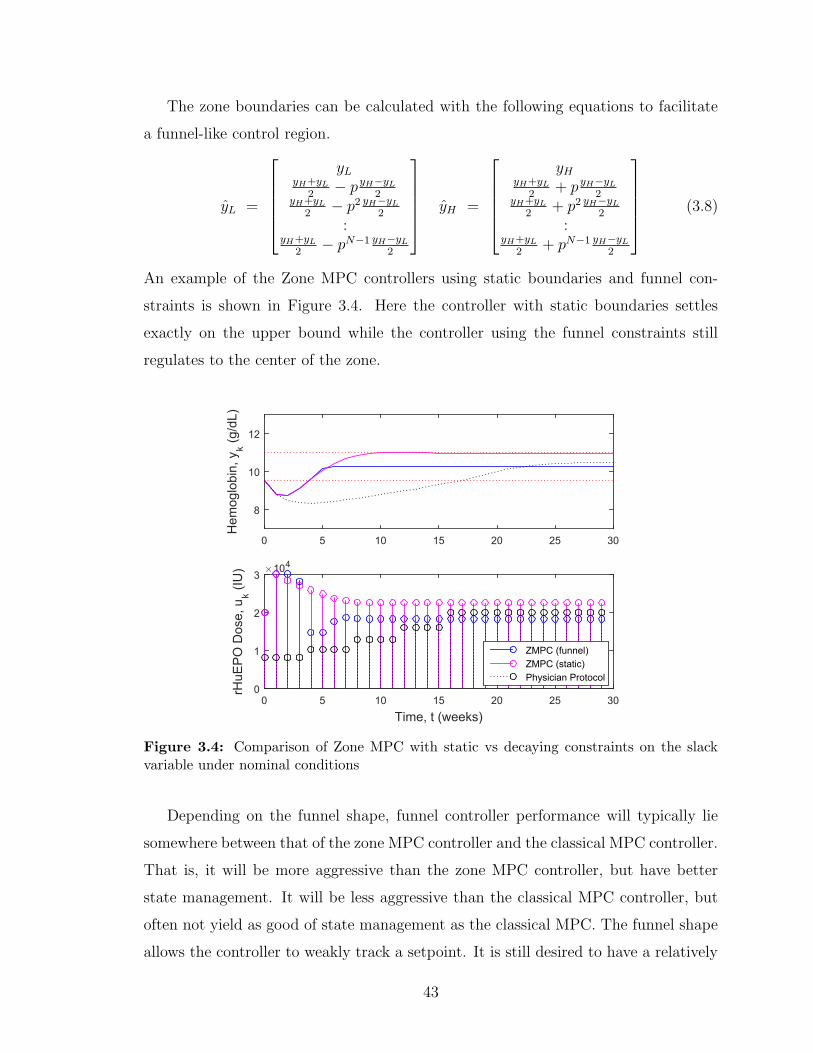
The zone boundaries can be calculated with the following equations to facilitate
a funnel-like control region.
yL =
yL
yH+yL2− pyH−yL
2yH+yL
2− p2 yH−yL
2
:yH+yL
2− pN−1 yH−yL
2
yH =
yH
yH+yL2
+ pyH−yL2
yH+yL2
+ p2 yH−yL2
:yH+yL
2+ pN−1 yH−yL
2
(3.8)
An example of the Zone MPC controllers using static boundaries and funnel con-
straints is shown in Figure 3.4. Here the controller with static boundaries settles
exactly on the upper bound while the controller using the funnel constraints still
regulates to the center of the zone.
0 5 10 15 20 25 30
Hem
oglo
bin,
yk (g
/dL)
8
10
12
Time, t (weeks)0 5 10 15 20 25 30
rHuE
PO
Dos
e, u
k (IU
) ×104
0
1
2
3
ZMPC (funnel)ZMPC (static)Physician Protocol
Figure 3.4: Comparison of Zone MPC with static vs decaying constraints on the slackvariable under nominal conditions
Depending on the funnel shape, funnel controller performance will typically lie
somewhere between that of the zone MPC controller and the classical MPC controller.
That is, it will be more aggressive than the zone MPC controller, but have better
state management. It will be less aggressive than the classical MPC controller, but
often not yield as good of state management as the classical MPC. The funnel shape
allows the controller to weakly track a setpoint. It is still desired to have a relatively
43
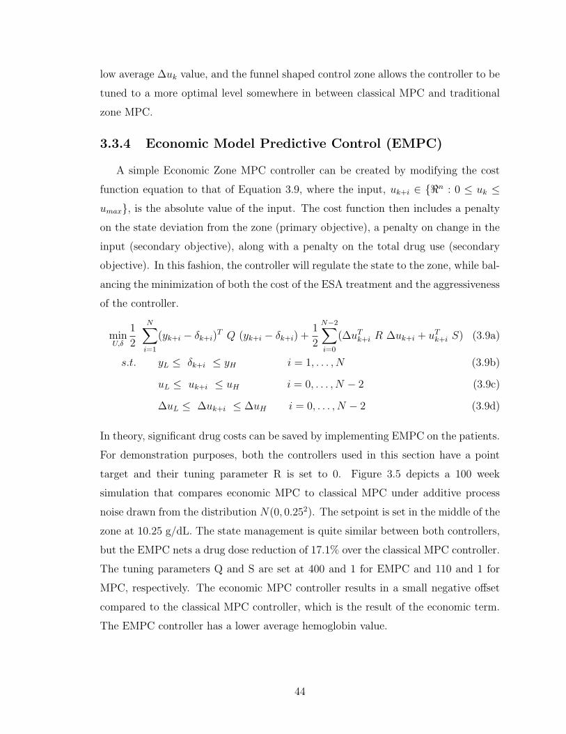
low average ∆uk value, and the funnel shaped control zone allows the controller to be
tuned to a more optimal level somewhere in between classical MPC and traditional
zone MPC.
3.3.4 Economic Model Predictive Control (EMPC)
A simple Economic Zone MPC controller can be created by modifying the cost
function equation to that of Equation 3.9, where the input, uk+i ∈ {<n : 0 ≤ uk ≤
umax}, is the absolute value of the input. The cost function then includes a penalty
on the state deviation from the zone (primary objective), a penalty on change in the
input (secondary objective), along with a penalty on the total drug use (secondary
objective). In this fashion, the controller will regulate the state to the zone, while bal-
ancing the minimization of both the cost of the ESA treatment and the aggressiveness
of the controller.
minU,δ
1
2
N∑i=1
(yk+i − δk+i)T Q (yk+i − δk+i) +
1
2
N−2∑i=0
(∆uTk+i R ∆uk+i + uTk+i S) (3.9a)
s.t. yL ≤ δk+i ≤ yH i = 1, . . . , N (3.9b)
uL ≤ uk+i ≤ uH i = 0, . . . , N − 2 (3.9c)
∆uL ≤ ∆uk+i ≤ ∆uH i = 0, . . . , N − 2 (3.9d)
In theory, significant drug costs can be saved by implementing EMPC on the patients.
For demonstration purposes, both the controllers used in this section have a point
target and their tuning parameter R is set to 0. Figure 3.5 depicts a 100 week
simulation that compares economic MPC to classical MPC under additive process
noise drawn from the distribution N(0, 0.252). The setpoint is set in the middle of the
zone at 10.25 g/dL. The state management is quite similar between both controllers,
but the EMPC nets a drug dose reduction of 17.1% over the classical MPC controller.
The tuning parameters Q and S are set at 400 and 1 for EMPC and 110 and 1 for
MPC, respectively. The economic MPC controller results in a small negative offset
compared to the classical MPC controller, which is the result of the economic term.
The EMPC controller has a lower average hemoglobin value.
44

0 10 20 30 40 50 60 70 80 90 100
Hem
oglo
bin,
yk (g
/dL)
8
10
12
Time, t (weeks)0 10 20 30 40 50 60 70 80 90 100
EP
O D
ose,
uk (
IU*1
0-3 )
0
10
20
30
MPCEMPCPhysician Protocol
Figure 3.5: Comparison of EMPC with classical MPC for a 100 week patient simulationusing additive process noise drawn from N(0, 0.252)
Figure 3.6a,b depicts two more simulations, when changing the tuning parameter
Q from 400 to 110 and 10000, respectively. The improper tuning parameters cause
significant offset to the downside of the system in Figure 3.6a. Figure 3.6b actually
shows the EMPC controller using more drug dose than the classical MPC controller,
a 4.4% increase.
0 10 20 30 40 50 60 70 80 90 100
Hem
oglo
bin,
yk (g
/dL)
8
10
12
Time, t (weeks)0 10 20 30 40 50 60 70 80 90 100
EP
O D
ose,
uk (
IU*1
0-3 )
0
10
20
30MPCEMPCPhysician Protocol
(a) EMPC Tuning Parameter Q=110
0 10 20 30 40 50 60 70 80 90 100
Hem
oglo
bin,
yk (g
/dL)
8
10
12
Time, t (weeks)0 10 20 30 40 50 60 70 80 90
EP
O D
ose,
uk (
IU*1
0-3 )
10
20
30MPCEMPCPhysician Protocol
(b) EMPC Tuning Parameter Q=10000
Figure 3.6: Simulations comparing different tuning parameters for the EMPC controller
Minimizing the drug costs in the cost function can be performed, but the tuning
parameters are highly sensitive. To aid in the tuning of this controller, the economic
term was changed to a linear term versus a quadratic term, and the doses are scaled
45

by 5000 IU. One of the complexities in tuning the controller is that drug doses come
in multiples of 1000 and range from 0 to as high as 40000 IU. With each patient
having different drug sensitivities, this controller becomes extremely difficult to tune
properly for each patient. If tuned incorrectly, the controller will jeopardize the
patients’ health. This controller will be explored further in Chapter 4.
3.3.5 Nonlinear Zone MPC
Another possible solution for control is through the use of a nonlinear Zone MPC
controller. This controller uses the PK/PD model from Equation 2.2 directly, and
coupled together with Matlab’s fmincon function, can solve for optimal control in-
puts. Nonlinear MPC has become more viable in recent years due to the advancement
in modern computational speed and efficiencies, but it is still quite computationally
expensive to solve a nonlinear programming problem (Allgower et al., 2004). Mat-
lab’s fmincon function uses an interior-point algorithm to solve this problem. The
algorithm simulates the system numerically, using a DDE solver similar to the one
developed in Chapter 2, and then calculates a new step size by estimating the gradi-
ent at that point. The numerical method for simulating the DDE model is again an
explicit method, so it does run the risk of being unstable for some time points which
would greatly impact the solution from fmincon.
Figure 3.7 depicts a short 100 week simulation using measurement and additive
process noise for the Nonlinear MPC controller versus a Linear MPC controller using
an ARX model. The PK/PD model is used to simulate the patient, which makes
almost identical models within the nonlinear MPC controller and the patient simula-
tor. The ARX model chosen for this simulation offers only a minor amount of plant
model mismatch, and does not produce a great deal of offset. In this simulation, the
measurement noise was drawn from a distribution of N(0, 0.1662) which corresponds
to a measurement error of approximately ±0.5 g/dL. The PK/PD model parameters
in the patient were also allowed to vary with each parameter following a distribution
of zero mean with the standard deviation being set to 10% of the original parameter
value. It is clear from the the simulation that the NMPC controller does not offer
improved accuracy over the linear counterpart. The time taken for the entire NMPC
controller for the 100 week simulation was 8.26 hours, while the linear MPC controller
46
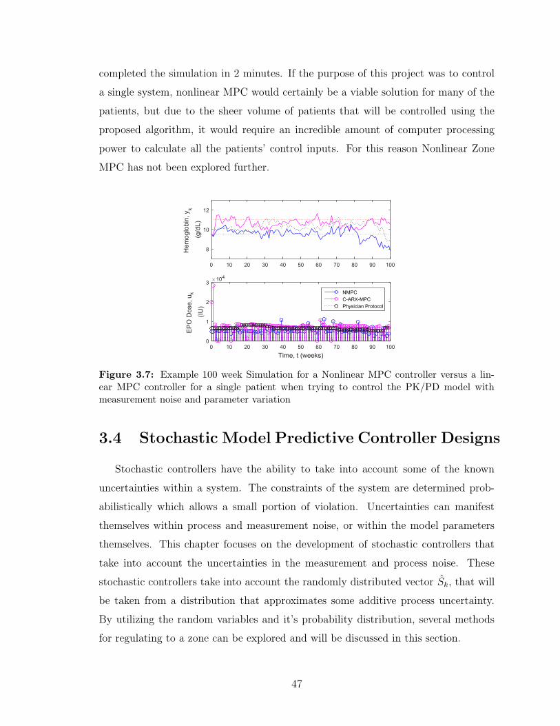
completed the simulation in 2 minutes. If the purpose of this project was to control
a single system, nonlinear MPC would certainly be a viable solution for many of the
patients, but due to the sheer volume of patients that will be controlled using the
proposed algorithm, it would require an incredible amount of computer processing
power to calculate all the patients’ control inputs. For this reason Nonlinear Zone
MPC has not been explored further.
0 10 20 30 40 50 60 70 80 90 100
Hem
oglo
bin,
yk
(g/d
L)
8
10
12
Time, t (weeks)0 10 20 30 40 50 60 70 80 90 100
E
PO
Dos
e, u
k
(IU)
×104
0
1
2
3
NMPCC-ARX-MPCPhysician Protocol
Figure 3.7: Example 100 week Simulation for a Nonlinear MPC controller versus a lin-ear MPC controller for a single patient when trying to control the PK/PD model withmeasurement noise and parameter variation
3.4 Stochastic Model Predictive Controller Designs
Stochastic controllers have the ability to take into account some of the known
uncertainties within a system. The constraints of the system are determined prob-
abilistically which allows a small portion of violation. Uncertainties can manifest
themselves within process and measurement noise, or within the model parameters
themselves. This chapter focuses on the development of stochastic controllers that
take into account the uncertainties in the measurement and process noise. These
stochastic controllers take into account the randomly distributed vector Sk, that will
be taken from a distribution that approximates some additive process uncertainty.
By utilizing the random variables and it’s probability distribution, several methods
for regulating to a zone can be explored and will be discussed in this section.
47
3.4.1 Stochastic System Model
Due to the propagation of error from each time instant along the prediction hori-
zon, the random vector Sk is multiplied to a variation of the state response matrix
which will be denoted as matrix D. Adding the additional random vector contribution
to the system, the model takes on the following form
yk = A yk + B uk + P Uk + D Sk (3.10)
where
D Sk =
I 0 · · · 0
(−a1) I · · · 0(−a1)2 (−a1) · · · 0
: :. . . :
(−a1)N−1 (−a1)N−2 · · · I
sksk+1
sk+2
:sk+N−1
3.4.2 Chance Constraints with Gaussian Uncertainty
The use of individual chance constraints was explored. In this method, these
constraints use the properties of the distribution of the random vector Sk and then
these chance constraints are formulated into hard constraints. If the random variables
inside the vector follow a Gaussian distribution they can be converted directly to
hard constraints (Grosso et al., 2014). If we consider the variable sk+i to be part of
the distribution N(s,Σ) where vector Dj refers to the jth row of the matrix D, the
hard constraints can be formulated from the following method (Grosso et al., 2014).
In zone control, chance constraints would be applied to both the upper and lower
bounds of the control region. For example purposes, the following upper bound
chance constraint will be used to illustrate the method.
Pr(yk+i < yH) ≥ 1− ε where yk+i = f(xk, uk, Uk) + DjSk (3.11)
In Equation (3.11), ε refers to the probability level in which the chance constraint is
allowed to be violated. The distribution of sk+i is not normal. To normalize this dis-
tribution in the chance constraint, it follows that the mean of the distribution should
be subtracted from both sides and then both sides can be divided by the standard
deviation of the distribution of the random variable DjSk+i (ie. N(sTDTj , DjΣD
Tj )).
48

The resulting equation is
Pr
DjSk − sTDTj√
DjΣDTj
<yH − f(xk, uk, Uk)− sTDT
j√DjΣDT
j
≥ 1− ε (3.12)
Equation (3.12) follows a standard normal distribution, N(0, 1), and can be
represented by
Φ
yH − f(xk, uk, Uk)− sTDTj√
DjΣDTj
≥ 1− ε (3.13)
where Φ (·) is the cumulative distribution function (CDF) of the standard normal
distribution. Taking the inverse CDF of both sides, and rearranging the equation
results in the deterministic hard constraint representing Equation (3.11)
yH ≥ φ−1(1− ε)√DjΣDT
j + sTDTj + f(xk, uk, Uk) (3.14)
Similarly, hard constraints can be determined for the lower zone boundary.
yL ≤ −φ−1(1− ε)√DjΣDT
j + sTDTj + f(xk, uk, Uk) (3.15)
Due to the constraints being hard constraints, the controller will naturally have
feasibility issues. This problem can be overcome by using a hybrid controller or
using soft constraints which will be discussed in the following sections.
3.4.3 Conditional Value at Risk (CVaR) Constraints
CVaR is a popular tool used in risk management. CVaR was introduced by Rock-
afellar and Uryasev (Rockafellar and Uryasev, 2000). It is widely used in the finance
industry for portfolio management. Before the advent of CVaR, the Value at Risk
(VaR) was the standard for optimization problems involving finances (Rockafellar
and Uryasev, 2000). In the finance industry, p−V aR is defined as the maximum loss
value that is assigned to some desired probability , p, over a given prediction horizon.
That is to mean that this loss p− V aR will occur p% of the time.
One of the main benefits over the previous chance constraint formulation, is that
CVaR is usable for any type of distribution and doesn’t rely on the noise distribution
being Gaussian. The following upper bound chance constraint will be used as an
49

example for the derivation of a CVaR constraint. Here, it is desired to have the
output remain underneath some upper bound within a certain probability. Opposite
to intuition, the following derivation is completed using a probability of violation (ε)
of the constraint. The uncertainty is again located within the output, yk, in the form
of a random variable sk+i. sk+i is part of the distribution N(s,Σ). For brevities sake
in notation, the output in the derivation will remain as yk and it will be assumed it
contains the random variable.
Pr{yk > yH} ≤ ε (3.16)
Equation 3.17 is the definition for the indicator function. This function holds a value
of 1 if u > 0 and a value of 0 if u ≤ 0.
1(0,∞)(u) = 1 if u > 0 (3.17a)
1(0,∞)(u) = 0 if u ≤ 0 (3.17b)
Inserting the positive variable α into the indicator function changes the input to the
indicator function but makes no difference in its output.
1(0,∞)(u) = 1(0,∞)(1
αu) (3.18a)
α > 0 (3.18b)
Defining an upper bounding function φ(u) for the indicator function, the following
inequality can be written.
1(0,∞)(1
αu) ≤ φ(
1
αu) (3.19)
Replacing u with yk − yH , the following inequality can be written. If yk − yH > 0
the constraint is violated and the indicator function holds a value of 1, and vice
versa. φ(u) is the upperbounding function for the indicator function and it is a
conservative estimate of the probability of violation, ε.
Pr{yk − yH > 0} = E[1(0,∞)(yk − yH)] ≤ E[φ(1
α(yk − yH))] ≤ ε (3.20)
50

From this, any solution that satisfies the inequality will also satisfy the constraint.
The focus will remain on the right side of this inequality. (u)+ is defined as the
maximum operator, which will hold the maximum value between 0 and the input u.
Applying the upper bounding function φ(u) = (u+ 1)+, a conservative
approximation of the chance constraint is defined as
E[( 1α
(yk − yH) + 1)+]≤ ε (3.21)
multiply by αε
1
εE[((yk − yH) + α)+
]≤ α (3.22)
moving α to the left hand side
−α +1
εE[((yk − yH) + α)+
]≤ 0 (3.23)
To reduce conservatism, find the minimum α that satisfies the inequality. That is, it
is desired to find the smallest upperbound. This results in the CVaR constraint, but
it is difficult to calculate its value in its present form.
minα−α +
1
εE[((yk − yH) + α)+
]≤ 0 (3.24)
The expectation operator is removed with the introduction of sampling to
approximate the CVaR constraint. M is the total number of scenarios. For instance,
if there were a single random variable per scenario, and the prediction horizon was
1, it would be necessary to sample the random variables’ distribution M times. πj is
the probability that a single scenario will occur, and will be equal to 1M
.
−α +1
ε
M∑j=1
πj[((yk,j − yH) + α)+
]≤ 0 (3.25)
The above equation is still not usable within an optimization constraint function. The
expression inside of the max operator can be replaced by two separate constraints.
The following equation replaces the max operator term with the variable vj, and con-
straints are set on vj to satisfy the original max operator’s function. The combination
of all three constraints in Equation 3.26 can be used to provide a conservative esti-
mate of the original chance constraint in Equation 3.16 through the use of sampling
(A. Parisio, 2013). These constraints are solved using many different scenarios of the
51

random variable distribution, leading to it being part of a class of controllers called
Scenario-Based MPC.
− α +1
ε
M∑j=1
πjvj ≤ 0 (3.26a)
vj ≥ (yk,j − yH) + α j = 1, ...,M (3.26b)
vj ≥ 0 j = 1, ...,M (3.26c)
3.4.4 Zone MPC Hybrid Controller using Hard Chance Con-straints
The controller outlined in this section uses the Quadratic Program formulation in
Equation 3.7, along with a number of chance constraints. The controller adds chance
constraints only when the system output enters the zone and the regular Zone MPC
controller is used while the output is outside of the desired zone. This controller
type leads to stable solutions but it reduces the ability to analytically explain the
probability of having the output within the bounds because the chance constraints
are not always used. It is typically not feasible for a large prediction horizon to have
a chance constraint at each time instant, k, along the predicted trajectory because
the constraints will end up converging at some point before the prediction horizon
ends making every solution infeasible. One way around this is to use less chance
constraints and then extend the final chance constraint to create a zone constraint
for the remaining portion of the prediction horizon. The constraint extension will not
be necessary in the control of hemoglobin because the prediction horizon is short and
does not allow the constraint convergence.
3.4.5 Zone MPC using Soft Chance Constraints
Another way to deal with the infeasibility of the chance constraints is to introduce
the addition of slack variables that relax the chance constraints if necessary. These
same slack variables are then penalized heavily in the cost function. In this way,
the relaxation of the constraints only occurs if the chance constraints are infeasible.
In these cases, the solution should then always touch the boundary of the relaxed
52

constraint. The hard constraints in Equations 3.14 and 3.15 with the introduction of
these slack variables become
yH + ξ1 > φ−1(1− ε)√DjΣDT
j + sTDTj + f(xk, uk, Uk) (3.27a)
yL − ξ2 < −φ−1(1− ε)√DjΣDT
j + sTDTj + f(xk, uk, Uk) (3.27b)
The Quadratic Program in Equation 3.7 can be augmented to include the two slack
variables ξ1 ∈ {<n : ξ1 > 0} and ξ2 ∈ {<n : ξ2 > 0}. The new H, f , and c will be
subscripted with 1 while the previous H, f , and c from Equation 3.7 will be used
without subscripts. The new penalty on the slack variables ξ1 and ξ2 will be
ξP ∈ {<n : ξP > 0} and hold a very high value.
minZk
1
2ZTk H1 Zk + fT1 Zk + c1 (3.28)
where
H1 =
H 0 00 ξP 00 0 ξP
and Zk =
ukδkξ1
ξ2
f1 =
[f 0 0
]Tc1 = c
Subject to the previous constraints as well as two new constraints on the new slack
variables
yL ≤ δk ≤ yH
uL ≤ uk ≤ uH
∆uL + uk ≤ φ uk ≤ ∆uH + uk
0 ≤ ξ1
0 ≤ ξ2
53

3.4.6 Scenario Based Zone MPC using Hard CVaR Con-straints
The controller described in this section belongs to the family of Scenario-Based
Controllers. The controller is designed to take into account an additive process noise
from a known distribution. Using this known distribution, the chance constraints
are created as outlined in Section 3.4.3. This controller design will have 2 CVaR
constraints on the output of the system, 1 on the lower bound and 1 on the upper
bound. The constraints will be used for k = 3 as shown in Equation 3.29.
− αk +1
ε
M∑j=1
πjvj,k ≤ 0 k = 3 (3.29a)
vj,k ≥ (yk,j − yH) + αk j = 1, ...,M, k = 3 (3.29b)
vj,k ≥ 0 j = 1, ...,M, k = 3 (3.29c)
− βk +1
ε
M∑j=1
πjωj,k ≤ 0 k = 3 (3.29d)
ωj,k ≥ (yL − yk,j) + βk j = 1, ...,M, k = 3 (3.29e)
ωj,k ≥ 0 j = 1, ...,M, k = 3 (3.29f)
The controller that will be tested for this section will use 100 scenarios (M = 100).
It should quickly become apparent that scenario-based constraints such as these lead
to a very large number of constraints. In this case, there will be 4M + 2 constraints
related to the CVaR constraints, leading to a total of 402 constraints. With this in
mind, the cost function used was changed to a linear program for the ability of that
solver type to handle a large number of constraints. In this case Matlab’s linprog
function was used along with its dual-simplex optimization solver. The cost function
is outlined in Equation 3.4.6.
minQ8∑
k=1
|yk − δk|+R
6∑k=0
|∆uk| (3.30)
This equation can be manipulated to remove the absolute sign and the resulting
linear program with all the constraints is outlined in Equation 3.31.
minQ8∑
k=1
hk +R6∑
k=0
gk (3.31a)
54
− αk +1
ε
M∑j=1
πjvj,k ≤ 0 k = 3 (3.31b)
vj,k ≥ (yk,j − yH) + αk j = 1, ...,M, k = 3 (3.31c)
vj,k ≥ 0 j = 1, ...,M, k = 3 (3.31d)
− βk +1
ε
M∑j=1
πjωj,k ≤ 0 k = 3 (3.31e)
ωj,k ≥ (yL − yk,j) + βk j = 1, ...,M, k = 3 (3.31f)
ωj,k ≥ 0 j = 1, ...,M, k = 3 (3.31g)
hk ≥ yk − δk k = 1, . . . , 8 (3.31h)
hk ≥ −(yk − δk) k = 1, . . . , 8 (3.31i)
gk ≥ ∆uk k = 0, . . . , 6 (3.31j)
gk ≥ −∆uk k = 0, . . . , 6 (3.31k)
δk ≤ yH k = 1, . . . , 8 (3.31l)
−δk ≤ −yL k = 1, . . . , 8 (3.31m)
uk ≤ Umax k = 0, . . . , 6 (3.31n)
−uk ≤ Umin k = 0, . . . , 6 (3.31o)
∆uk ≤ ∆Umax k = 0, . . . , 6 (3.31p)
−∆uk ≤ ∆Umin k = 0, . . . , 6 (3.31q)
55

Equation 3.31 leads to a total of 470 constraints and an optimization vector Zk as
outlined below. There are 2M + 30 variables to be optimized (232).
Zk =
u0
:u6
δ1
:δ8
α3
:v1,3
:v100,3
β3
ω1,3
:ω100,3
h1
:h8
g0
:g6
(3.32)
Due to in-feasibility issues, if the controller fails to find a feasible solution, a backup
classical MPC controller will be used for that time instant. This is a hybrid controller
solution similar to that used in the controller with Hard Chance Constraints.
3.4.7 Scenario Based Zone MPC using Soft CVaR Constraints
Similar to the formulation for soft constraints previously mentioned in the Gaus-
sian case, the CVaR constraints can be relaxed to facilitate feasibility. Again, a slack
variable is introduced to relax the constraints in Equation 3.33b,e. The constraints in
Equation 3.33r,s are also added to ensure the new slack variables are always positive.
minQ8∑
k=1
hk +R6∑
k=0
gk + ξP (ξ1 + ξ2) (3.33a)
− ξ1 − αk +1
ε
M∑j=1
πjvj,k ≤ 0 k = 3 (3.33b)
vj,k ≥ (yk,j − yH) + αk j = 1, ...,M, k = 3 (3.33c)
56

vj,k ≥ 0 j = 1, ...,M, k = 3 (3.33d)
− ξ2 − βk +1
ε
M∑j=1
πjωj,k ≤ 0 k = 3 (3.33e)
ωj,k ≥ (yL − yk,j) + βk j = 1, ...,M, k = 3 (3.33f)
ωj,k ≥ 0 j = 1, ...,M, k = 3 (3.33g)
hk ≥ yk − δk k = 1, . . . , 8 (3.33h)
hk ≥ −(yk − δk) k = 1, . . . , 8 (3.33i)
gk ≥ ∆uk k = 0, . . . , 6 (3.33j)
gk ≥ −∆uK k = 0, . . . , 6 (3.33k)
δk ≤ yH k = 1, . . . , 8 (3.33l)
−δk ≤ −yL k = 1, . . . , 8 (3.33m)
uk ≤ Umax k = 0, . . . , 6 (3.33n)
−uk ≤ Umin k = 0, . . . , 6 (3.33o)
∆uk ≤ ∆Umax k = 0, . . . , 6 (3.33p)
−∆uk ≤ ∆Umin k = 0, . . . , 6 (3.33q)
ξ1 ≥ 0 (3.33r)
ξ2 ≥ 0 (3.33s)
3.4.8 Scenario Based Zone MPC using Conditional Value atRisk in Cost Function
Another controller method for dealing with uncertainty is the scenario based MPC
controller using CVaR in the cost function, rather than in the constraints. The con-
troller discussed here, will look at optimizing the control inputs using conditional
value at risk, directly within the cost function which leads to a solution that is al-
ways feasible. The scenario based Zone MPC controller uses the distribution of the
random variable sk to generate several different plausible scenarios of noise. Instead
of optimizing a linear or quadratic objective as before, the controller optimizes the
Conditional Value at Risk (β-CVaR) as introduced by Bemporady et al (Bemporady
et al., 2011). The formulation of this problem requires several steps and starts with
57

the definition of a linear program similar to the previous quadratic objective function
used. The linear program used as the loss function is ∈ <n+i which is associated with
decision vectors uk ∈ {<n : umin ≤ uk ≤ umax} and δk ∈ {<n : yL ≤ δk ≤ yH} and
random vector Sk ∈ <n. Uk ∈ <n is associated with the past inputs. Note that Q
and R are again used as the tuning parameters in this equation.
f(uk, Uk, δk, Sk) = QN∑i=1
|yk+i − δk+i| + R
N−2∑i=0
|∆uk+i| (3.34)
Let p(s) be the probability density function of the random variable sk. Used in the
calculation of β-CVaR is another parameter β-VaR (Value at Risk) which is defined
as the smallest value for which the probability that the loss function will not exceed
its value is β. β is the fixed value confidence level and typically holds a value
greater than 0.9. The downside of using only β-VaR (`) is that the loss greater than
` is not accounted for. β-CVaR allows for the quantification of losses greater than `.
The variable β-VaR is defined as
`β(uk, Uk, δk) = min{` ∈ < : ψ(uk, Uk, δk, `) ≥ β} (3.35)
where the probability of f(uk, Uk, δk, Sk) not exceeding ` is
(uk, Uk, δk, `) =
∫f(uk,Uk,δk,Sk)≤`
p(s)ds (3.36)
β-CVaR is defined as
φβ(uk, Uk, δk) = (1− β)−1
∫f(uk,Uk,δk,Sk)≥`β(u)
f(uk, Uk, δk, Sk) p(s)ds (3.37)
The loss associated with any uk , Uk and δk can be determined from the addition of
both β-VaR and β-CVaR.
Fβ(uk, Uk, δk, `) = `+ (1− β)−1
∫Sk∈<m
[f(uk, Uk, δk, Sk)− `]+p(s)ds (3.38)
[f ]+ denotes the max of [f, 0]. The integral in the above equation is difficult to solve
explicitly which brings about the need to perform sampling to approximate it. M
number of scenarios (or M vectors of Sk) are randomly generated from p(s) with
each scenario having a probability of πj of occurring. Then Equation (3.38) can be
approximated by
58
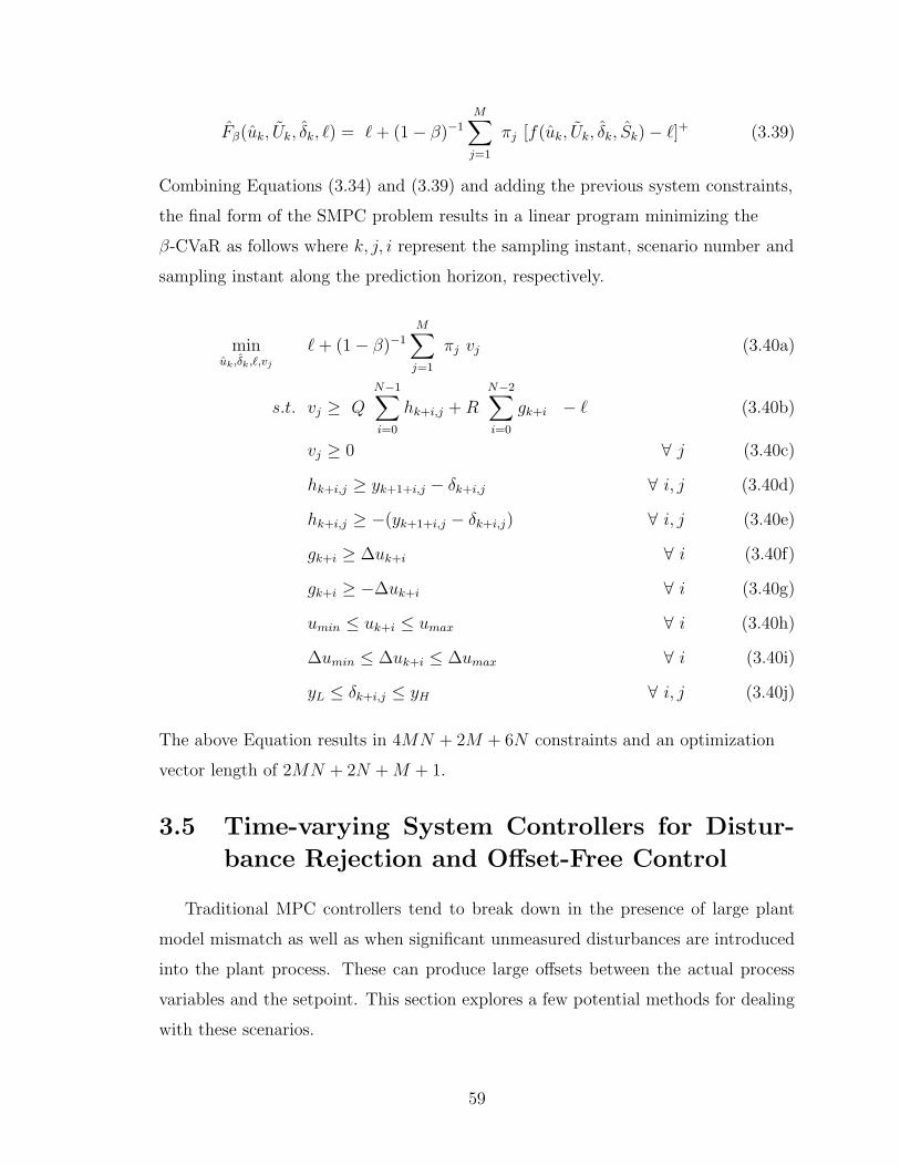
Fβ(uk, Uk, δk, `) = `+ (1− β)−1
M∑j=1
πj [f(uk, Uk, δk, Sk)− `]+ (3.39)
Combining Equations (3.34) and (3.39) and adding the previous system constraints,
the final form of the SMPC problem results in a linear program minimizing the
β-CVaR as follows where k, j, i represent the sampling instant, scenario number and
sampling instant along the prediction horizon, respectively.
minuk,δk,`,vj
`+ (1− β)−1
M∑j=1
πj vj (3.40a)
s.t. vj ≥ QN−1∑i=0
hk+i,j +RN−2∑i=0
gk+i − ` (3.40b)
vj ≥ 0 ∀ j (3.40c)
hk+i,j ≥ yk+1+i,j − δk+i,j ∀ i, j (3.40d)
hk+i,j ≥ −(yk+1+i,j − δk+i,j) ∀ i, j (3.40e)
gk+i ≥ ∆uk+i ∀ i (3.40f)
gk+i ≥ −∆uk+i ∀ i (3.40g)
umin ≤ uk+i ≤ umax ∀ i (3.40h)
∆umin ≤ ∆uk+i ≤ ∆umax ∀ i (3.40i)
yL ≤ δk+i,j ≤ yH ∀ i, j (3.40j)
The above Equation results in 4MN + 2M + 6N constraints and an optimization
vector length of 2MN + 2N +M + 1.
3.5 Time-varying System Controllers for Distur-
bance Rejection and Offset-Free Control
Traditional MPC controllers tend to break down in the presence of large plant
model mismatch as well as when significant unmeasured disturbances are introduced
into the plant process. These can produce large offsets between the actual process
variables and the setpoint. This section explores a few potential methods for dealing
with these scenarios.
59

3.5.1 ZMPC with Internal Model Control and Integrator
The first such method is a simple version of offset-free MPC. The aim of this
controller was to explore a way to deal with plant-model mismatch as well as any un-
modeled disturbances. It is already known that most patients’ health will deteriorate
slowly overtime, similar to the introduction of a slow continuous ramp disturbance.
The idea behind this MPC algorithm is to calculate the 1-step error between the
ARX model and the actual measurement and adjust the reference targets for the
zone boundaries to reflect the estimate for the estimated steady state offset (alterna-
tively one could include the disturbance estimate Dk in the model instead of adjusting
the targets). Offset-Free MPC algorithms similar to this have been shown to work
well for constant steady state disturbances (Pannocchia and Rawlings, 2003). This
method can be expressed in the following equations in terms of deviation variables.
The ARX model is in the form
yk = a1yk−1 +20∑i=1
biuk−i + Dk−1 (3.41)
and gives a 1-step ahead estimate of the system when using the past data on and
before time k − 1.
dk = yk − yk (3.42)
gives an estimate for the 1-step residual at time k. This residual is multiplied by a
filter value, K, and added to the summation of the previous time step estimate for
dk. Equation 3.5.1 represents the total integrated output 1-step error.
Dk =k∑1
Kdk (3.43)
The model inside the controller remains static, but the targets of the MPC routine
are adjusted to reflect the steady state offset estimate. This is represented by
yL,new = yL − Dk (3.44a)
yH,new = yH − Dk (3.44b)
A block diagram of the simulation setup is shown in Figure 3.8. The DDE solver
along with a random additive disturbance is used as the patient simulator. The DDE
60

solver is in continuous time and sampled weekly, while the designed control system is
in discrete time with a sampling interval equal to the hemoglobin sampling rate. In
cases of constant steady state offset, this algorithm will capture the full offset over
time.
Figure 3.8: Block Diagram of the MPC and IMC algorithm with a filtered integrator whensimulated using a disturbance variable and measurement noise
Figure 3.9 shows a 500 week simulation where an additive noise disturbance ac-
cumulates a negative sum in the first 250 weeks and then switches to accumulating a
positive sum in the last 250 weeks. The filter value K is equal to 0.2, 0.5 and 0.8 in
these simulations. The low filter value helps to reject any acute disturbances and zero
mean measurement noise but still captures the long-term disturbance dynamics. As
the filter value increases, the input response becomes much noiser, and the gains in
state management are minimal. The shortcomings of this configuration can be seen
in this figure. In cases of steady ramp disturbances such as the simulation in Figure
3.9, this algorithm will often lag behind the actual disturbance, as can be seen in the
middle of the simulation where the system settles on or below the control zone limit.
This lag presents a large problem for the time-varying nature of the steady state EPO
dose. It is likely that the steady state dose may oscillate up and down over the course
of the patient’s life. The IMC configuration works well for steady state offset, but
fails to provide adequate control when the steady-state dose changes quickly. For this
61

reason, the IMC configuration was not explored further in the following chapters.
0 50 100 150 200 250 300 350 400 450 500
Hem
oglo
bin,
yk(g
/dL)
7
8
9
10
11
12
13
0 50 100 150 200 250 300 350 400 450 500
E
PO
Dos
e, u
k(IU
)
×104
0
0.5
1
1.5
2
2.5
3
MPCOF-MPC 0.2Physician ProtocolOF-MPC 0.5OF-MPC 0.8
Time, t(weeks)0 50 100 150 200 250 300 350 400 450 500
Dis
turb
ance
, Dk (g
/DL)
-4
-2
0
2
4
Figure 3.9: Comparison of different filter values with an Offset-Free MPC controller versusa classical MPC controller for a single patient when trying to control the PK/PD modelwith uncertainties
3.5.2 ZMPC with Recursive Modeling
To overcome the dynamic nature of a patients’ health over time, this algorithm
recursively estimates a new constrained ARX model at each specified time instant.
This method relies on the fixed structure of the C-ARX models to ensure that the
model attained at each time step is open-loop stable and representative of a physio-
logically acceptable model (Turksoy et al., 2014). The estimation phase uses a moving
window of historical data that is 50 data points in length. A longer window is typi-
cally better for model estimation, but patient health may change over time, making
the initial data counter-productive in estimating a present time model. If too little
data is used, it is difficult mathematically to find a proper solution, given the large
number of degrees of freedom in the model. A block diagram of the simulation is
shown in Figure 3.10 . The controller model, steady states, and constraints must be
updated after each new model is obtained.
62
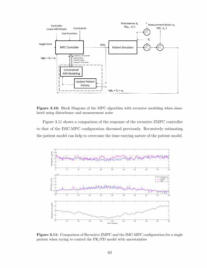
Figure 3.10: Block Diagram of the MPC algorithm with recursive modeling when simu-lated using disturbance and measurement noise
Figure 3.11 shows a comparison of the response of the recursive ZMPC controller
to that of the IMC-MPC configuration discussed previously. Recursively estimating
the patient model can help to overcome the time-varying nature of the patient model.
0 50 100 150 200 250 300 350 400 450 500
Hem
oglo
bin,
yk(g
/dL)
7
8
9
10
11
12
13
0 50 100 150 200 250 300 350 400 450 500
E
PO
Dos
e, u
k(IU
)
×104
0
0.5
1
1.5
2
2.5
3
OF-MPC 0.2R-ZMPCAMP
Time, t(weeks)0 50 100 150 200 250 300 350 400 450 500
Dis
turb
ance
, Dk (g
/DL)
-4
-2
0
2
4
Figure 3.11: Comparison of Recursive ZMPC and the IMC-MPC configuration for a singlepatient when trying to control the PK/PD model with uncertainties
63

3.5.3 Digital PID Control
Another appropriate method for control is to use a Digital PID controller. PID
control is a very mature technology and used widely across many industries. PID
controllers have the advantage of being able to be tuned for disturbance rejection
which may offer improved state management in scenarios where the patient model is
time-varying. PID controllers have been used successfully in the control of Type 1
Diabetes and the first FDA approved automatic insulin pump (Medtronic’s Minimed
670G, approved by FDA Sept 28, 2016) is equipped with PID control (S. Trevitt,
2016). PID controllers typically perform quite well for SISO systems, if designed and
tuned properly (O’Dwyer, 2006).
To design the PID controllers, a First Order Plus Deadtime (FOPDT) transfer
function estimate for the patient model is first needed. Due to health consequences
and liabilities, it is not feasible to perform step tests on the patients in practice. One
method to derive a FOPDT model is to first estimate a Constrained ARX model,
and subsequently perform a step test on the attained model. The steady state values
from the C-ARX model identification will be used for the FOPDT model. The dosing
levels are chosen appropriately to center the step response over the control zone,
having the initial hemoglobin approximately equal to 9.5 and the final hemoglobin
appropriately equal to 11 g/dL. In order to identify the FOPDT model automatically,
the dosing levels are chosen automatically through the use of a simple Interval Halving
Optimization Method. The deadtime (θ) for each system will be assumed to be 2
weeks to avoid having to get the tangent line to the curve in the transfer function
estimate. Using linear interpolation between the simulated data points, and the
beginning and final simulated measurements, a FOPDT model can be easily attained
automatically using the a graphical method outlined in Figure 3.12.
64
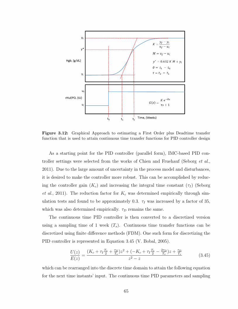
Figure 3.12: Graphical Approach to estimating a First Order plus Deadtime transferfunction that is used to attain continuous time transfer functions for PID controller design
As a starting point for the PID controller (parallel form), IMC-based PID con-
troller settings were selected from the works of Chien and Fruehauf (Seborg et al.,
2011). Due to the large amount of uncertainty in the process model and disturbances,
it is desired to make the controller more robust. This can be accomplished by reduc-
ing the controller gain (Kc) and increasing the integral time constant (τI) (Seborg
et al., 2011). The reduction factor for Kc was determined empirically through sim-
ulation tests and found to be approximately 0.3. τI was increased by a factor of 35,
which was also determined empirically. τD remains the same.
The continuous time PID controller is then converted to a discretized version
using a sampling time of 1 week (Ts). Continuous time transfer functions can be
discretized using finite difference methods (FDM). One such form for discretizing the
PID controller is represented in Equation 3.45 (V. Bobal, 2005).
U(z)
E(z)=
(Kc + τITs2
+ τDTs
)z2 + (−Kc + τITs2− 2τD
Ts)z + τD
Ts
z2 − z(3.45)
which can be rearranged into the discrete time domain to attain the following equation
for the next time instants’ input. The continuous time PID parameters and sampling
65
time (in weeks) are substituted into the equation.
u(k) = u(k−1)+(Kc+τITs2
+τDTs
)e(k)+(−Kc+τITs2−2τDTs
)e(k−1)+τDTse(k−2) (3.46)
3.6 Conclusion
Several model based predictive controllers were designed and discussed in this
chapter. Two main classifications of controllers were explored, deterministic and
stochastic. Deterministic controllers do not take into account the possible uncer-
tainty in the measurements and process noise. The stochastic controllers are able to
take into account these uncertainties and should be more effective than their deter-
ministic counterparts when the uncertainty distributions are known. The stochastic
controllers introduced here however, do not take into account parameter uncertainty.
It is possible that plant model mismatch may adversely affect these controller types.
Three methods for dealing with the Time-varying nature of the models were pre-
sented. These included the internal model control based MPC, Recursive MPC and
Digital PID controller methods. The IMC based MPC will not be explored further
due to its inability to provide good control for ramp disturbances. The PID con-
troller and the recursive ZMPC algorithm will be tested rigorously, under different
simulation scenarios in Chapter 4.
66

Chapter 4
Simulation Results and Discussion
4.1 Introduction
This Chapter focuses on many aspects of the controller simulation results. The
first section uses the C-ARX models within the MPC controllers, and performs sev-
eral test scenarios to determine the effectiveness of the MPC controllers against one
another as well as against the current anemia management protocol obtained from
an actual hemodialysis unit from a hospital.
The first set of simulations will focus on the controller algorithms. The ARX
models will be used in the both the controller and as the patient simulator. The
tuning parameters for each controller will first be discussed. The controllers will be
tested using different types of disturbances and process noise. These tests represent
the nominal case and will provide good results to eliminate some of the less effective
controllers designed in Chapter 3.
The last section includes simulation results which represent a more realistic test
scenario, where the controllers are used to control the PK/PD model as it is subjected
to process noise and disturbances. These simulations use a designed patient simulator
which includes measurement noise, integrating process disturbance noise as well as
random acute disturbances. The random integrating disturbance causes the average
patient dose to drift away from its original value. The random acute disturbances
simulate infections and blood loss which are common to CKD patients. To overcome
the time-varying nature of the patient simulator, recursive modeling will be used.
The chapter will conclude with the final recommendation for the control system.
67
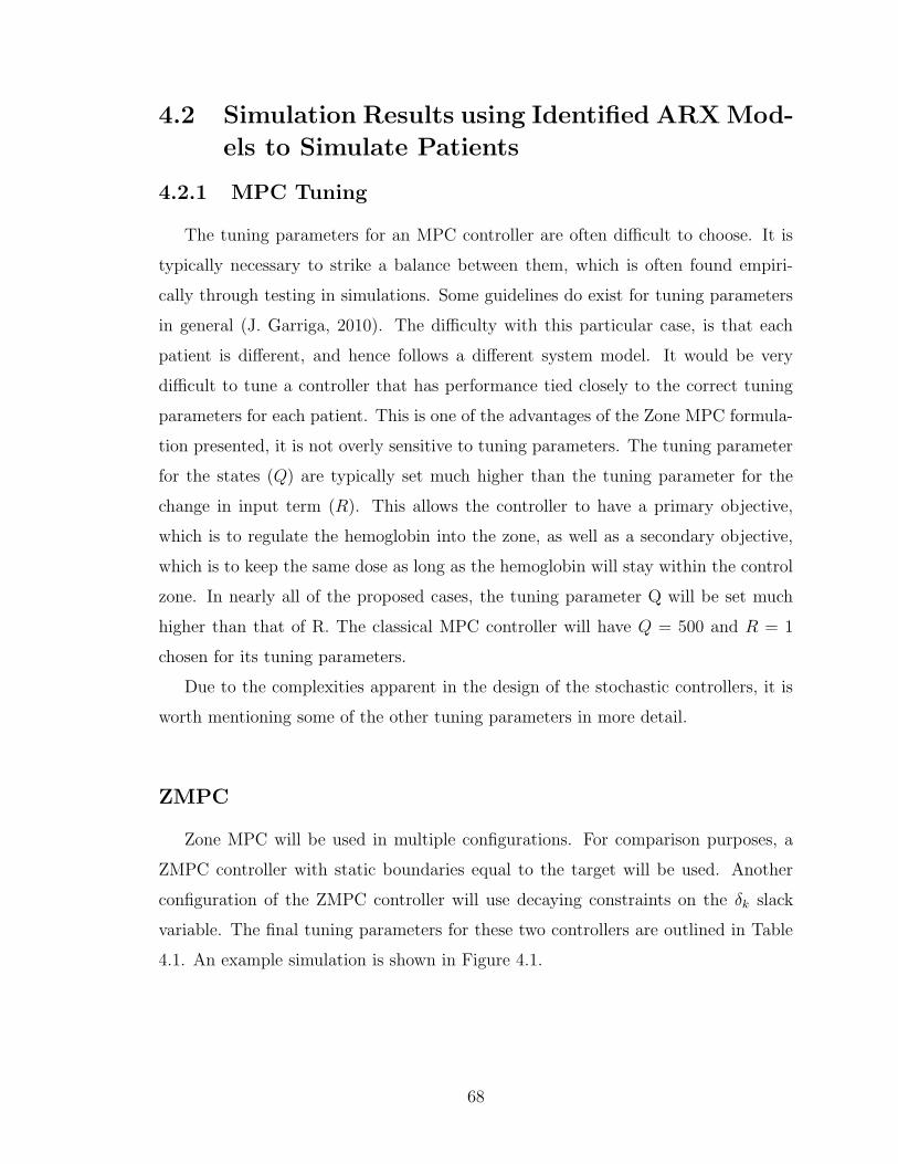
4.2 Simulation Results using Identified ARX Mod-
els to Simulate Patients
4.2.1 MPC Tuning
The tuning parameters for an MPC controller are often difficult to choose. It is
typically necessary to strike a balance between them, which is often found empiri-
cally through testing in simulations. Some guidelines do exist for tuning parameters
in general (J. Garriga, 2010). The difficulty with this particular case, is that each
patient is different, and hence follows a different system model. It would be very
difficult to tune a controller that has performance tied closely to the correct tuning
parameters for each patient. This is one of the advantages of the Zone MPC formula-
tion presented, it is not overly sensitive to tuning parameters. The tuning parameter
for the states (Q) are typically set much higher than the tuning parameter for the
change in input term (R). This allows the controller to have a primary objective,
which is to regulate the hemoglobin into the zone, as well as a secondary objective,
which is to keep the same dose as long as the hemoglobin will stay within the control
zone. In nearly all of the proposed cases, the tuning parameter Q will be set much
higher than that of R. The classical MPC controller will have Q = 500 and R = 1
chosen for its tuning parameters.
Due to the complexities apparent in the design of the stochastic controllers, it is
worth mentioning some of the other tuning parameters in more detail.
ZMPC
Zone MPC will be used in multiple configurations. For comparison purposes, a
ZMPC controller with static boundaries equal to the target will be used. Another
configuration of the ZMPC controller will use decaying constraints on the δk slack
variable. The final tuning parameters for these two controllers are outlined in Table
4.1. An example simulation is shown in Figure 4.1.
68

Tuning Parameter static funnelQ 500 500R 1 1yL (δk constraint) 9.5 g/dL 9.75 g/dLyH (δk constraint) 11 g/dL 10.75 g/dLyL (target) 9.5 g/dL 9.5 g/dLyH (target) 11 g/dL 11 g/dLp, (yL decay ratio on δk constraint) 0 0.6p, (yH decay ratio on δk constraint) 0 0.6
Table 4.1: Final tuning settings for the ZMPC controllers that will be tested
0 10 20 30 40 50 60 70 80 90 100
Hem
oglo
bin,
yk (g
/dL)
8
10
12
Time (weeks)0 10 20 30 40 50 60 70 80 90 100
EP
O D
ose,
uk (I
U)
×104
0
1
2
3ZMPC (funnel)ZMPC (static)Physician Protocol
Figure 4.1: Example simulation comparing ZMPC with static boundaries and decayingboundaries on the δk constraints
ZMPC Hybrid with 1 CVaR Constraint
The first controller discussed here is the ZMPC controller with CVaR constraints.
This controller requires an estimate for the process noise distribution to draw random
samples from, for the scenarios. It also requires tuning parameters Q and R, along
with control zone boundaries for the constraints, as well as control zone boundaries
for δk. The number of scenarios M and the CVaR constraint violation probability ε
is also needed. It should be noted that the CVaR constraints cannot be combined
with a ZMPC controller that has a control boundary larger than what the CVaR con-
straints will typically be solved as, because this eliminates the state term in the cost
69
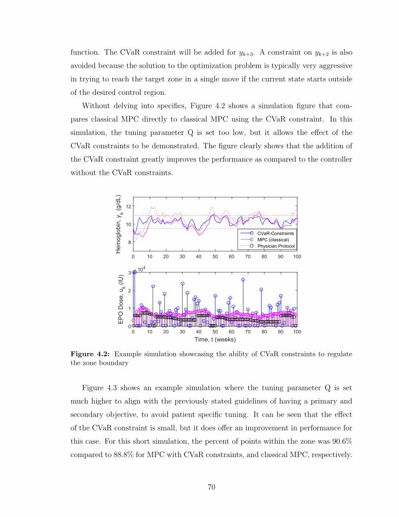
function. The CVaR constraint will be added for yk+3. A constraint on yk+2 is also
avoided because the solution to the optimization problem is typically very aggressive
in trying to reach the target zone in a single move if the current state starts outside
of the desired control region.
Without delving into specifics, Figure 4.2 shows a simulation figure that com-
pares classical MPC directly to classical MPC using the CVaR constraint. In this
simulation, the tuning parameter Q is set too low, but it allows the effect of the
CVaR constraints to be demonstrated. The figure clearly shows that the addition of
the CVaR constraint greatly improves the performance as compared to the controller
without the CVaR constraints.
0 10 20 30 40 50 60 70 80 90 100
Hem
oglo
bin,
yk (g
/dL)
8
10
12
Time, t (weeks)0 10 20 30 40 50 60 70 80 90 100
E
PO
Dos
e, u
k (IU
)
×104
0
1
2
3
CVaR-ConstraintsMPC (classical)Physician Protocol
Figure 4.2: Example simulation showcasing the ability of CVaR constraints to regulatethe zone boundary
Figure 4.3 shows an example simulation where the tuning parameter Q is set
much higher to align with the previously stated guidelines of having a primary and
secondary objective, to avoid patient specific tuning. It can be seen that the effect
of the CVaR constraint is small, but it does offer an improvement in performance for
this case. For this short simulation, the percent of points within the zone was 90.6%
compared to 88.8% for MPC with CVaR constraints, and classical MPC, respectively.
70
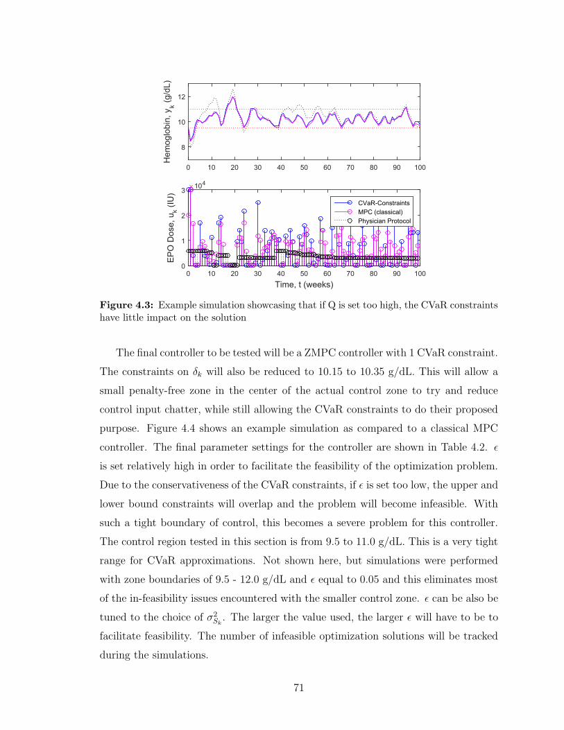
0 10 20 30 40 50 60 70 80 90 100H
emog
lobi
n, y
k (g/d
L)
8
10
12
Time, t (weeks)0 10 20 30 40 50 60 70 80 90 100
E
PO
Dos
e, u
k (IU
)
×104
0
1
2
3
CVaR-ConstraintsMPC (classical)Physician Protocol
Figure 4.3: Example simulation showcasing that if Q is set too high, the CVaR constraintshave little impact on the solution
The final controller to be tested will be a ZMPC controller with 1 CVaR constraint.
The constraints on δk will also be reduced to 10.15 to 10.35 g/dL. This will allow a
small penalty-free zone in the center of the actual control zone to try and reduce
control input chatter, while still allowing the CVaR constraints to do their proposed
purpose. Figure 4.4 shows an example simulation as compared to a classical MPC
controller. The final parameter settings for the controller are shown in Table 4.2. ε
is set relatively high in order to facilitate the feasibility of the optimization problem.
Due to the conservativeness of the CVaR constraints, if ε is set too low, the upper and
lower bound constraints will overlap and the problem will become infeasible. With
such a tight boundary of control, this becomes a severe problem for this controller.
The control region tested in this section is from 9.5 to 11.0 g/dL. This is a very tight
range for CVaR approximations. Not shown here, but simulations were performed
with zone boundaries of 9.5 - 12.0 g/dL and ε equal to 0.05 and this eliminates most
of the in-feasibility issues encountered with the smaller control zone. ε can be also be
tuned to the choice of σ2Sk
. The larger the value used, the larger ε will have to be to
facilitate feasibility. The number of infeasible optimization solutions will be tracked
during the simulations.
71

Tuning Parameter ValueQ 100R 1yL (δk constraint) 10.05 g/dLyH (δk constraint) 10.45 g/dLyL (target) 9.5 g/dLyH (target) 11 g/dLM 100ε 0.25Sk *σ2Sk
*
Table 4.2: Final tuning settings for the ZMPC-CVaR (constraint) controller that will betested.
*note the mean and variance of the random distribution will be set during specificsimulation tests
0 10 20 30 40 50 60 70 80 90 100
Hem
oglo
bin,
yk (g
/dL)
8
10
12
Time, t (weeks)0 10 20 30 40 50 60 70 80 90 100
E
PO
Dos
e, u
k (IU
)
×104
0
1
2
3ZMPC-CVaR (Constraints)MPC (classical)Physician Protocol
Figure 4.4: Example simulation using the final controller tuning settings for the ZMPC-CVaR (constraints) controller to be tested as compared to classical MPC
ZMPC with 1 Soft CVaR Constraint
This controller is exactly the same as the previous controller using a CVaR con-
straint on time instant yk+3, but instead of using a backup controller in the event
of in-feasibility, an additional slack variable will be used to loosen the constraints to
make the problem feasible when necessary. The slack variable will then be penalized
72
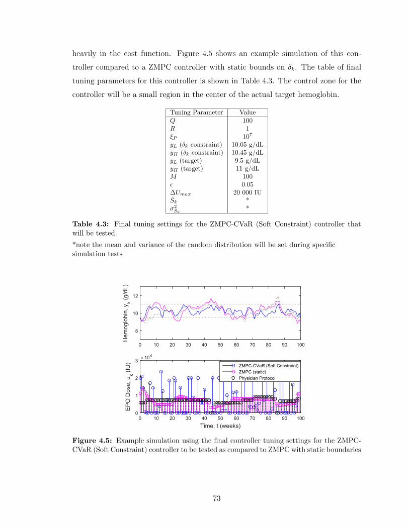
heavily in the cost function. Figure 4.5 shows an example simulation of this con-
troller compared to a ZMPC controller with static bounds on δk. The table of final
tuning parameters for this controller is shown in Table 4.3. The control zone for the
controller will be a small region in the center of the actual target hemoglobin.
Tuning Parameter ValueQ 100R 1ξP 107
yL (δk constraint) 10.05 g/dLyH (δk constraint) 10.45 g/dLyL (target) 9.5 g/dLyH (target) 11 g/dLM 100ε 0.05∆Umax 20 000 IUSk *σ2Sk
*
Table 4.3: Final tuning settings for the ZMPC-CVaR (Soft Constraint) controller thatwill be tested.
*note the mean and variance of the random distribution will be set during specificsimulation tests
0 10 20 30 40 50 60 70 80 90 100
Hem
oglo
bin,
yk (g
/dL)
8
10
12
Time, t (weeks)0 10 20 30 40 50 60 70 80 90 100
EP
O D
ose,
uk (I
U)
×104
0
1
2
3ZMPC-CVaR (Soft Constraint)ZMPC (static)Physician Protocol
Figure 4.5: Example simulation using the final controller tuning settings for the ZMPC-CVaR (Soft Constraint) controller to be tested as compared to ZMPC with static boundaries
73

ZMPC with CVaR in the Cost Function
This controller, unlike it’s CVaR constraint counterpart, is always feasible. It
is not necessary to use a backup controller. This controller is still a scenario-based
controller and uses the linear program over the quadratic program due to its large
number of constraints. An example simulation of the ZMPC-CVaR (Cost) controller
as compared to a ZMPC controller is shown in Figure 4.6. Here both zone boundary
conditions on δk are equal to the target zone of 9.5-11 g/dL. The ZMPC-CVaR (Cost)
controller regulates the points in the zone at an accuracy of 93.0%, compared to that
of the ZMPC controller with 72.2%. One thing to note is the aggressiveness of the
controller. This controller exhibits the largest average changes in the input out of all
the controllers discussed. For this reason, a constraint on ∆Uk is also used to cap the
changes to a max of 20000 IU.
0 10 20 30 40 50 60 70 80 90 100
Hem
oglo
bin,
yk (g
/dL)
8
10
12
Time, t (weeks)0 10 20 30 40 50 60 70 80 90 100
E
PO
Dos
e, u
k (IU
)
×104
0
1
2
3
ZMPC-CVaR (Cost)ZMPC (static)Physician Protocol
Figure 4.6: Example simulation using the final controller tuning settings for the ZMPC-CVaR (Cost) controller to be tested as compared to ZMPC with static boundaries
The final tuning parameters for this controller are outlined in Table 4.4.
74

Tuning Parameter ValueQ 100R 1yL (δk constraint) 10.05 g/dLyH (δk constraint) 10.45 g/dLyL (target) 9.5 g/dLyH (target) 11 g/dLM 200β 0.99∆Umax 20 000 IUSk *σ2Sk
*
Table 4.4: Final tuning settings for the ZMPC-CVaR (cost) controller that will be tested.
*note the mean and variance of the random distribution will be set during specificsimulation tests
ZMPC Hybrid with 7 Hard Chance Constraints
This controller will use the standard ZMPC controller formulation with the addi-
tion of 7 chance constraints on yk+2 to yk+8. There was no chance constraint placed
on yk+1 as it cannot be affected by uk. Due to the nature of the hard constraints,
a backup classical MPC controller will be used in case the optimization problem be-
comes infeasible. Figure 4.7 shows the controller as compared to a ZMPC controller
with again the same boundaries used on δk that are equal to the target zone of 9.5 to
11.0 g/dL.
0 10 20 30 40 50 60 70 80 90 100
Hem
oglo
bin,
yk (g
/dL)
8
10
12
Time, t (weeks)0 10 20 30 40 50 60 70 80 90 100
EP
O D
ose,
Uk (I
U)
×104
0
1
2
3
ZMPC-HCCZMPC (static)Physician Protocol
Figure 4.7: Example simulation using the final controller tuning settings for the ZMPC-HCC (7) to be tested as compared to ZMPC with static boundaries
75

For the final tuning parameters, the constraints on yL and yH will decrease expo-
nentially to create a funnel. Figure 4.8 shows an example of the δk constraints and
chance constraints visually.
Prediction Horizon, N (weeks)1 2 3 4 5 6 7 8
Hem
oglo
bin,
yk (g
/dL)
8
8.5
9
9.5
10
10.5
11
11.5
12
Chance Constraint Boundaryδ
k Constraint Boundary
Figure 4.8: Example simulation using the final controller tuning settings for the ZMPC-HCC (7) to be tested as compared to ZMPC with static boundaries
The final tuning parameters that will be used for this controller are outlined in
Table 4.5. The constraints on δk will decay back towards the center of the zone at
the ratio specified.
Tuning Parameter ValueQ 500R 1yL (δk constraint) 9.75 g/dLyH (δk constraint) 10.75 g/dLyL decay ratio (δk constraint) 0.6k g/dLyH decay ratio (δk constraint) 0.6k g/dLyL (target) 9.5 g/dLyH (target) 11 g/dLε 0.01Sk *σ2Sk
*
Table 4.5: Final tuning settings for the ZMPC-HCC (7) controller that will be tested.
*note the mean and variance of the random distribution will be set during specificsimulation tests
76
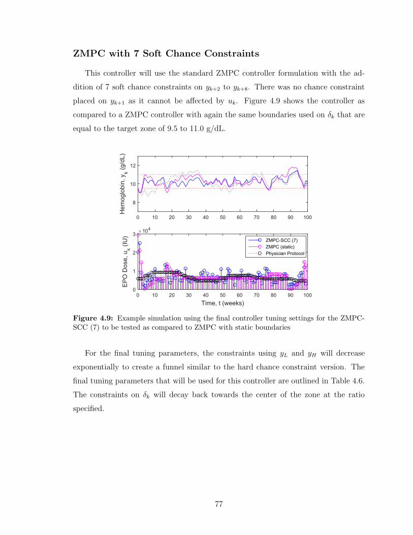
ZMPC with 7 Soft Chance Constraints
This controller will use the standard ZMPC controller formulation with the ad-
dition of 7 soft chance constraints on yk+2 to yk+8. There was no chance constraint
placed on yk+1 as it cannot be affected by uk. Figure 4.9 shows the controller as
compared to a ZMPC controller with again the same boundaries used on δk that are
equal to the target zone of 9.5 to 11.0 g/dL.
0 10 20 30 40 50 60 70 80 90 100
Hem
oglo
bin,
yk (g
/dL)
8
10
12
Time, t (weeks)0 10 20 30 40 50 60 70 80 90 100
EP
O D
ose,
uk (I
U)
×104
0
1
2
3ZMPC-SCC (7)ZMPC (static)Physician Protocol
Figure 4.9: Example simulation using the final controller tuning settings for the ZMPC-SCC (7) to be tested as compared to ZMPC with static boundaries
For the final tuning parameters, the constraints using yL and yH will decrease
exponentially to create a funnel similar to the hard chance constraint version. The
final tuning parameters that will be used for this controller are outlined in Table 4.6.
The constraints on δk will decay back towards the center of the zone at the ratio
specified.
77
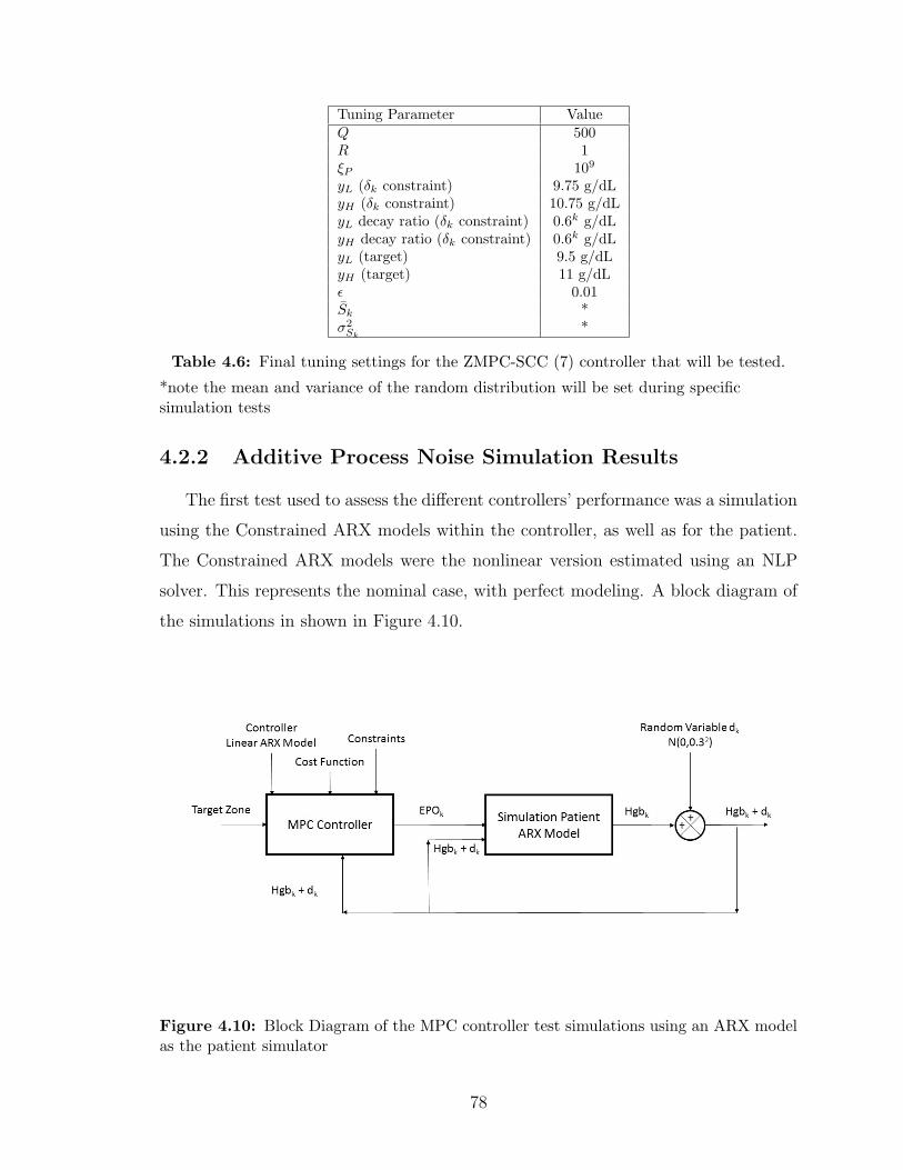
Tuning Parameter ValueQ 500R 1ξP 109
yL (δk constraint) 9.75 g/dLyH (δk constraint) 10.75 g/dLyL decay ratio (δk constraint) 0.6k g/dLyH decay ratio (δk constraint) 0.6k g/dLyL (target) 9.5 g/dLyH (target) 11 g/dLε 0.01Sk *σ2Sk
*
Table 4.6: Final tuning settings for the ZMPC-SCC (7) controller that will be tested.
*note the mean and variance of the random distribution will be set during specificsimulation tests
4.2.2 Additive Process Noise Simulation Results
The first test used to assess the different controllers’ performance was a simulation
using the Constrained ARX models within the controller, as well as for the patient.
The Constrained ARX models were the nonlinear version estimated using an NLP
solver. This represents the nominal case, with perfect modeling. A block diagram of
the simulations in shown in Figure 4.10.
Figure 4.10: Block Diagram of the MPC controller test simulations using an ARX modelas the patient simulator
78

These results are shown in Table 4.7. The additive process noise was drawn from
a distribution of sk = N(0, 0.32) and added to the system output after each week of
simulation. In practical applications, the hemoglobin value is not expected to change
more than 5% between actual hemoglobin measurements (1 week intervals), making
this noise distribution near the worst case scenario. Simulations were performed
across all 167 patient models for 500 weeks. Due to some of the patient models not
being acceptable, the results were filtered. The models were estimated using Matlab’s
fmincon function and there are no guarantees that a global minimum solution has
been found. There are also no guarantees that each patient’s data was acceptable
to estimate a model. Many of the patients are also healthy enough to not receive
epoetin-alfa for many weeks, which could result in a bad model. The results were
filtered by removing all the simulations for every patient that scored less than 50%
of the points within the zone for at least one of the controllers or the physician’s
protocol. Filtering with this criteria, the statistics in the table include 132 of the 167
patients. This aids in excluding models that do not behave like actual patients, and
can skew the results, especially in the physician protocol statistics. Another item to
note, is that the stochastic controllers were given the exact distribution of additive
noise, which may not be realistic in actual practice.
PerformanceStatistic
MPC ZMPC ZMPC ZMPC ZMPC ZMPC ZMPC ZMPC AMPclass. static funnel SCC HCC H-CVaR S-CVaR CVaR
(7) (7) (1) (1) (cost)Integrated yk Err. 0.136 0.314 0.186 0.141 0.142 0.164 0.162 0.194 0.486% of Points in Zone 92.0 82.5 89.1 91.6 91.4 90.5 90.3 89.5 76.1
Uk Total ( IU1000
) 4724 4714 4699 4708 4690 4754 4738 4782 4909Avg. Weekly Uk 9448.7 9428 9398 9416 9380 9509 9476 9564 9817Avg. ∆Uk 4684 423 487 3178 2424 4609 7751 8165 344
Table 4.7: Simulation Results for the various ZMPC controllers as compared to the physi-cian’s protocol for the additive process noise test scenario
There are many observations that can be concluded within these simulation re-
sults. One of the first things to note, is that the average change in the input is
extremely conservative for the physician’s protocol. This is due to the protocol not
allowing the change of inputs very often. Usually the dose is changed, and then not
allowed to be changed again for 2-4 weeks. The model based controllers will likely
change the dose often as they respond to disturbances and process noise.
The first controller to be discussed is the classical MPC controller. The classi-
79

cal MPC controller is seen to have the highest accuracy in state control. With the
tuning parameter, Q, set abnormally high, this result makes sense. The classical
controller does however suffer by having very high average drug use, along with very
high average ∆uk as compared to the other controllers. The state performance of
this controller could be considered close to the upper limit that any of the controllers
could achieve within the problem constraints.
The ZMPC controller with static boundaries on the slack variable, δk, performs
better but quite similar to the Physician Protocol in all categories. It has small im-
provements in all categories reducing the Integrated Output Error by 35.5% and the
total drug use by 4.0%. The percent of points was 8.4% higher and this comes at a
cost of increasing the average change in input by only 23.0%. However, this controller
remains the most sluggish controller, of all the model based controllers tested, due to
the large control zone. Zone MPC typically lags in state performance with regards
to setpoint based MPC controllers (B. Grosman, 2010), but its benefits come in the
form of a more clinically acceptable and safer controller due to the more constant
drug doses.
The ZMPC controller with funnel constraints on the slack variable, δk, performs
much better than the ZMPC controller in terms of state control and total drug use.
Adding the funnel constraint offers large improvements over static boundaries. As
compared to the physician’s protocol, it offers improvements in every category except
increasing the average weekly change in dose by only 41.6%, which is still minimal
compared to the other controllers. The funnel control zone allows the weak tracking
of a setpoint, while also retaining some of the features of the Zone MPC algorithm
with the static control zone boundaries.
The two ZMPC controllers using the chance constraints converted to hard con-
straints assuming Gaussian uncertainty perform similar to each other. These con-
trollers use chance constraints on the upper and lower zone boundary for k + 2 to
k + 8. ZMPC HCC (7) is the hybrid controller that uses classical MPC in the event
of infeasibility. The HCC version of the controller becomes infeasible around 2% of
the time. ZMPC SCC (7), relaxes the constraints until they are feasible, with these
relaxation variables being penalized heavily in the cost function. These controllers
also use the same funnel constraints as the ZMPC funnel controller. Both of these
80
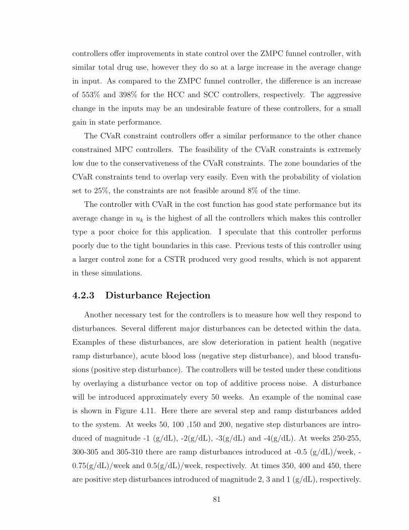
controllers offer improvements in state control over the ZMPC funnel controller, with
similar total drug use, however they do so at a large increase in the average change
in input. As compared to the ZMPC funnel controller, the difference is an increase
of 553% and 398% for the HCC and SCC controllers, respectively. The aggressive
change in the inputs may be an undesirable feature of these controllers, for a small
gain in state performance.
The CVaR constraint controllers offer a similar performance to the other chance
constrained MPC controllers. The feasibility of the CVaR constraints is extremely
low due to the conservativeness of the CVaR constraints. The zone boundaries of the
CVaR constraints tend to overlap very easily. Even with the probability of violation
set to 25%, the constraints are not feasible around 8% of the time.
The controller with CVaR in the cost function has good state performance but its
average change in uk is the highest of all the controllers which makes this controller
type a poor choice for this application. I speculate that this controller performs
poorly due to the tight boundaries in this case. Previous tests of this controller using
a larger control zone for a CSTR produced very good results, which is not apparent
in these simulations.
4.2.3 Disturbance Rejection
Another necessary test for the controllers is to measure how well they respond to
disturbances. Several different major disturbances can be detected within the data.
Examples of these disturbances, are slow deterioration in patient health (negative
ramp disturbance), acute blood loss (negative step disturbance), and blood transfu-
sions (positive step disturbance). The controllers will be tested under these conditions
by overlaying a disturbance vector on top of additive process noise. A disturbance
will be introduced approximately every 50 weeks. An example of the nominal case
is shown in Figure 4.11. Here there are several step and ramp disturbances added
to the system. At weeks 50, 100 ,150 and 200, negative step disturbances are intro-
duced of magnitude -1 (g/dL), -2(g/dL), -3(g/dL) and -4(g/dL). At weeks 250-255,
300-305 and 305-310 there are ramp disturbances introduced at -0.5 (g/dL)/week, -
0.75(g/dL)/week and 0.5(g/dL)/week, respectively. At times 350, 400 and 450, there
are positive step disturbances introduced of magnitude 2, 3 and 1 (g/dL), respectively.
81

From weeks 450-500, there exists a negative ramp disturbance of -0.1 (g/dL)/week. It
is interesting to note that the physician’s protocol can induce an oscillatory behavior
in the output. The hemoglobin control of the physician’s protocol is not very good
and results in a lot of hemoglobin values over the 11.0 g/dL zone target. Hemoglobin
values above the upper limit of the target zone are undesirable and result in the use of
excess epoetin-alfa, which has economic consequences. The disturbances here are also
well spread out in time with almost a year in between the disturbances. Patients may
undergo more disturbances within a shorter time limit, which could further impact
control. The MPC algorithms are easily able to deal with these acute disturbances
and return the hemoglobin to the target zone.
0 50 100 150 200 250 300 350 400 450 500
Hem
oglo
bin,
yk (g
/dL)
8
10
12
Time, t (weeks)0 50 100 150 200 250 300 350 400 450 500
E
PO
Dos
e, u
k (IU
)
×104
0
1
2
3
CVaR Constraints Hard (1)CVaR CostZMPC HCC (6)ZMPC SCC (6)ZMPC (funnel)ZMPC (static)MPC (classical)CVaR Constraints Soft (1)Physician Protocol
Figure 4.11: Example simulation of the controller response to the designed output dis-turbance # 1 vector for the nominal case (no process noise)
Applying this identical disturbance to patient number 15, along with an additive
process noise of N(0, 0.252) results in the controller responses shown in Figure 4.12.
82
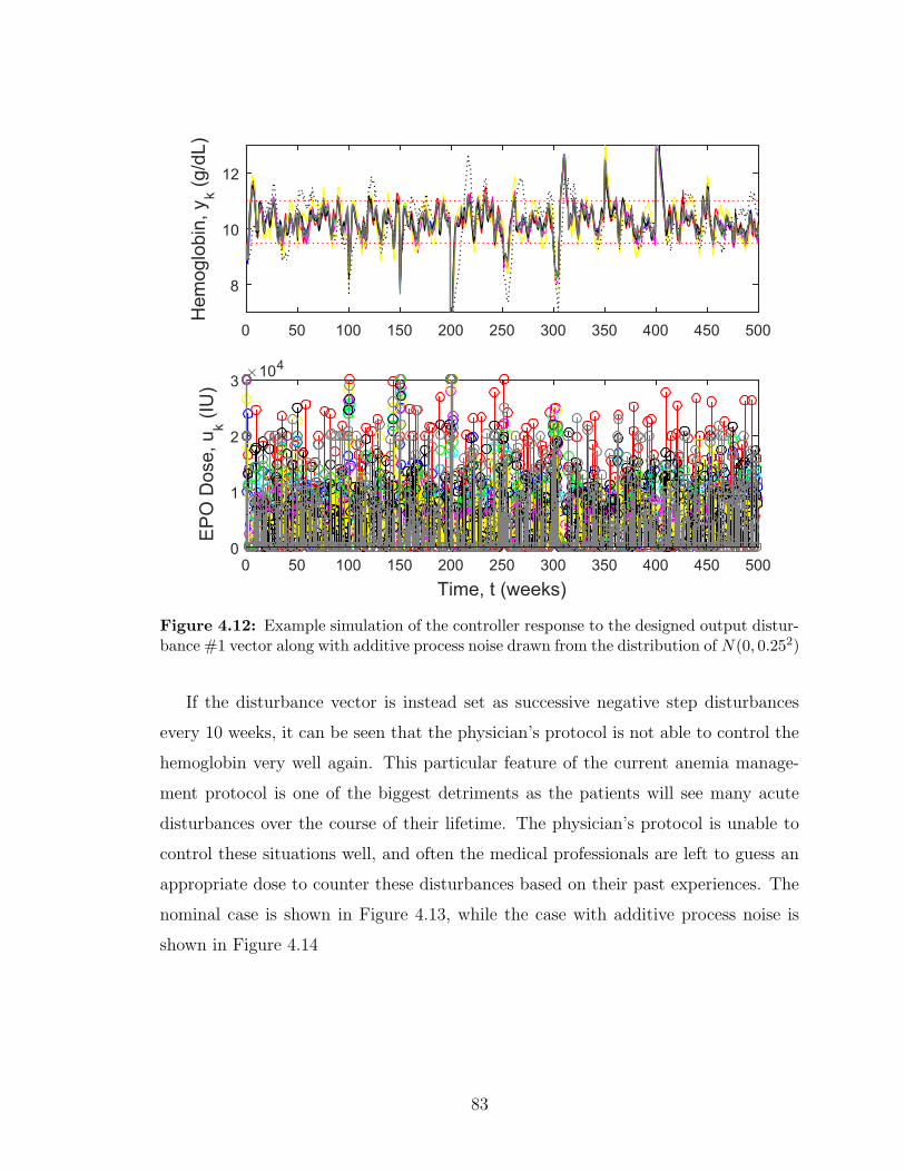
0 50 100 150 200 250 300 350 400 450 500
Hem
oglo
bin,
yk (g
/dL)
8
10
12
Time, t (weeks)0 50 100 150 200 250 300 350 400 450 500
E
PO
Dos
e, u
k (IU
)
×104
0
1
2
3
Figure 4.12: Example simulation of the controller response to the designed output distur-bance #1 vector along with additive process noise drawn from the distribution of N(0, 0.252)
If the disturbance vector is instead set as successive negative step disturbances
every 10 weeks, it can be seen that the physician’s protocol is not able to control the
hemoglobin very well again. This particular feature of the current anemia manage-
ment protocol is one of the biggest detriments as the patients will see many acute
disturbances over the course of their lifetime. The physician’s protocol is unable to
control these situations well, and often the medical professionals are left to guess an
appropriate dose to counter these disturbances based on their past experiences. The
nominal case is shown in Figure 4.13, while the case with additive process noise is
shown in Figure 4.14
83

0 50 100 150
Hem
oglo
bin,
yk (g
/dL)
8
10
12
Time, t (weeks)0 50 100 150
E
PO
Dos
e, u
k (IU
)
×104
0
1
2
3
CVaR Constraints Hard (1)CVaR CostZMPC HCC (6)ZMPC SCC (6)ZMPC (funnel)ZMPC (static)MPC (classical)CVaR Constraints Soft (1)Physician Protocol
Figure 4.13: Example simulation of the controller responses to successive negative stepdisturbances for the nominal case (no process noise)
Again, the same disturbance can be applied along with an additive process noise
from the distribution N(0, 0.252). Figure 4.14 shows the controller responses for
patient 15 for this case. The AMP spends a lot more time outside the control zone
boundary than the model predictive controllers. The state performance between most
of the controllers is very similar.
84
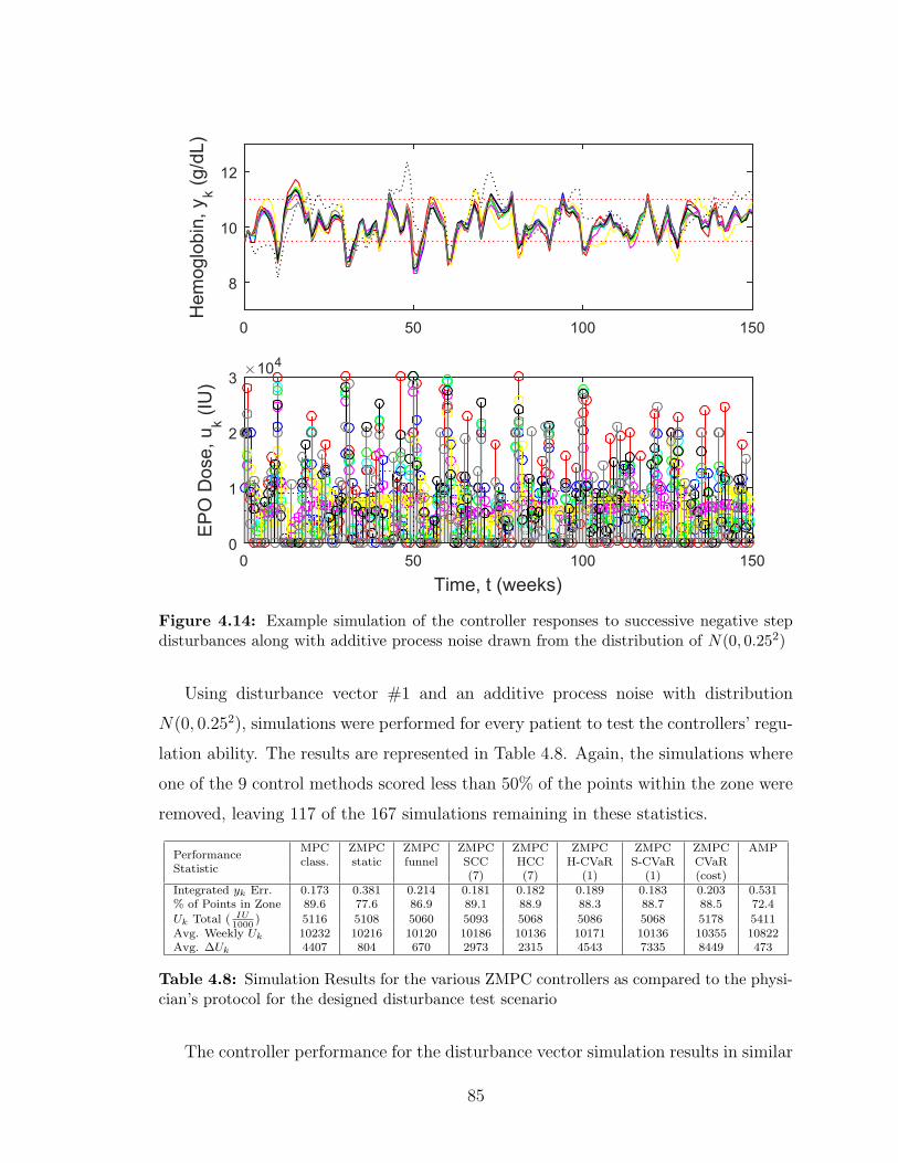
0 50 100 150
Hem
oglo
bin,
yk (g
/dL)
8
10
12
Time, t (weeks)0 50 100 150
E
PO
Dos
e, u
k (IU
)
×104
0
1
2
3
Figure 4.14: Example simulation of the controller responses to successive negative stepdisturbances along with additive process noise drawn from the distribution of N(0, 0.252)
Using disturbance vector #1 and an additive process noise with distribution
N(0, 0.252), simulations were performed for every patient to test the controllers’ regu-
lation ability. The results are represented in Table 4.8. Again, the simulations where
one of the 9 control methods scored less than 50% of the points within the zone were
removed, leaving 117 of the 167 simulations remaining in these statistics.
PerformanceStatistic
MPC ZMPC ZMPC ZMPC ZMPC ZMPC ZMPC ZMPC AMPclass. static funnel SCC HCC H-CVaR S-CVaR CVaR
(7) (7) (1) (1) (cost)Integrated yk Err. 0.173 0.381 0.214 0.181 0.182 0.189 0.183 0.203 0.531% of Points in Zone 89.6 77.6 86.9 89.1 88.9 88.3 88.7 88.5 72.4
Uk Total ( IU1000
) 5116 5108 5060 5093 5068 5086 5068 5178 5411Avg. Weekly Uk 10232 10216 10120 10186 10136 10171 10136 10355 10822Avg. ∆Uk 4407 804 670 2973 2315 4543 7335 8449 473
Table 4.8: Simulation Results for the various ZMPC controllers as compared to the physi-cian’s protocol for the designed disturbance test scenario
The controller performance for the disturbance vector simulation results in similar
85

performance values for each of the controllers as compared to the simulations without
the disturbance vector. As expected, each of the controllers state management dete-
riorates slightly due to the acute disturbances. The ZMPC controller with the funnel
constraints offers the most desirable solution. It has very good state performance,
coupled with a very low average change in uk. The chance constrained controllers (as
tuned) have good state performance, but the rate change terms are far too high to be
considered viable in a clinical setting. The Zone MPC (static and funnel) controllers
will be studied further in more rigorous simulation tests.
4.3 Controller Simulation Results on PK/PD Pa-
tient Simulator
In order to test the controllers with a more realistic scenario, it is proposed to
test the controllers’ regulation abilities when trying to control the PK/PD model,
along with added process , measurement noise and acute disturbances. The following
sections outline the design of a realistic patient simulator, justification for the chosen
noise distributions and the simulation results on the patient simulator.
A block diagram of the simulation setup is shown in Figure 4.15.
4.3.1 Patient Simulator Design
To begin the control system testing, simulated data was needed initially to acquire
a constrained ARX model of the system. As in a clinical setting, an initial few months
of data is necessary before a proper model can be identified for the MPC algorithms
to be put into use. Initially, the PK/PD models were used along with a designed
disturbance, random measurement noise and the physician’s protocol control scheme
to collect simulated data. A constrained ARX model was subsequently identified
from this simulated data. An example of this is shown in Figure 4.16 for both the
validation and training data. The data was split evenly into training and validation
portions, similar to the clinical data. The bottom subplot, shows the shape of the bk
parameters.
86

Figure 4.15: Block Diagram of the Simulation Setup for Recursive Zone Model PredictiveControl and the Patient Simulator
Figure 4.16: Example of a scenario used to attain the C-ARX models from simulated data
Model parameters were estimated for each of the 167 clinical patients and it is these
models that serve as the basis for the simulated patients. The actual clinical patients
exhibit many varying degrees of behaviour beyond that which the PK/PD model can
87

capture. Most notably, clinical patients may become increasingly dependent on EPO
over time. This can be seen in a few clinical patients in Figure 4.17.
0 100 200 300 400 500 600 700 800 900 1000
Hgb
, (g/
dL)
6
8
10
12
Time (days)0 100 200 300 400 500 600 700 800 900 1000
E
PO
(IU
)
0
5000
10000
15000
(a) Patient 4
0 100 200 300 400 500 600 700 800 900 1000
Hgb
, (g/
dL)
8
10
12
14
Time (days)0 100 200 300 400 500 600 700 800 900 1000
E
PO
(IU
)
×104
0
0.5
1
1.5
2
(b) Patient 5
0 100 200 300 400 500 600 700 800 900 1000
Hgb
, (g/
dL)
8
10
12
14
Time (days)0 100 200 300 400 500 600 700 800 900 1000
E
PO
(IU
)
0
2000
4000
6000
8000
(c) Patient 6
Figure 4.17: Clinical patients will become continually more dependent on EPO doses iftheir natural endogenous erythropoietin production deteriorates
Some patients may also become more healthy for short periods of time. This
phenomena is depicted in multiple patients in Figure 4.18.
0 100 200 300 400 500 600 700 800 900 1000
Hgb
, (g/
dL)
6
8
10
12
14
Time (days)0 100 200 300 400 500 600 700 800 900 1000
E
PO
(IU
)
×104
0
0.5
1
1.5
2
(a) Patient 7
0 100 200 300 400 500 600 700 800 900 1000
Hgb
, (g/
dL)
9
10
11
12
Time (days)0 100 200 300 400 500 600 700 800 900 1000
E
PO
(IU
)
0
5000
10000
(b) Patient 8
0 100 200 300 400 500 600 700 800 900 1000
Hgb
, (g/
dL)
8
10
12
14
Time (days)0 100 200 300 400 500 600 700 800 900 1000
E
PO
(IU
)×104
0
0.5
1
1.5
2
(c) Patient 9
Figure 4.18: Clinical patients become less dependent on EPO doses as their naturalendogenous erythropoietin production increases
Both of these scenarios bring about a time varying nature of the process system.
To aid in simulating these conditions, an integrating disturbance with a small negative
mean was used. This allows the patients’ hemoglobin response to drift slowly away
from the original model in either direction, but with a bias to the downside. The
accumulation of the disturbance term will impact the steady state input significantly.
Another frequent occurrence is acute negative step and ramp disturbances. These
can be seen during infections or when significant blood loss occurs. Some acute
disturbances can be seen in the clinical patients shown in Figure 4.19. The step
disturbances are clearly identifiable. Patient 10 exhibits a negative ramp disturbance
around day 800. Patient 12 exhibits a negative ramp disturbance around day 375.
88

0 100 200 300 400 500 600 700 800 900 1000H
gb, (
g/dL
)
6
8
10
12
14
Time (days)0 100 200 300 400 500 600 700 800 900 1000
E
PO
(IU
)×104
0
0.5
1
1.5
2
(a) Patient 10
0 100 200 300 400 500 600 700 800 900 1000
Hgb
, (g/
dL)
6
8
10
12
Time (days)0 100 200 300 400 500 600 700 800 900 1000
E
PO
(IU
)
×104
0
1
2
3
4
(b) Patient 11
0 100 200 300 400 500 600 700 800 900 1000
Hgb
, (g/
dL)
6
8
10
12
14
Time (days)0 100 200 300 400 500 600 700 800 900 1000
E
PO
(IU
)
×104
0
1
2
3
4
(c) Patient 12
Figure 4.19: Clinical patients’ exhibiting acute disturbances
The occurrence of these types of disturbances is also incorporated into the patient
simulator. A negative step or ramp disturbance can be incorporated by modifying
the red blood cell population. Low weekly probabilities are given to these types of
disturbances making them occur randomly. The RBC population is represented by
the 2, 3 and 4th states in the PKPD model. The probability of a step disturbance
occurring is set to 1 % each week. This results in approximately one acute step
disturbance event per 2 years, per patient. There is a 15 week grace period after
each step disturbance where another disturbance cannot occur, to avoid multiple
disturbances in very short periods of time. The magnitude of the step disturbance is
randomly chosen to reduce the current red blood cell population by multiplying it by a
fractional number between 0.73 and 0.98. This disturbance translates to a maximum
hemoglobin drop of roughly -3.5 g/dL, which is near the maximum drop observed in
the clinical data. The states governing the RBC population can be modified using
Equations 4.1, which are derived in the original work on the PKPD model (Chait et
al., 2014). The new RBC population is calculated incorporating the step disturbance
(AD). AD holds a value of 1 unless a disturbance is selected for the current weekly
time instance. If a disturbance is selected, AD is set to a fractional value and Rk
is updated. The state x2 is also updated to reflect changes in the RBC population.
States x1,k and Ek remain unchanged.
Rk,new = ADRk (4.1a)
x2,k = Rk,new −4x1,k
µ(4.1b)
Similarly, negative ramp disturbances are also programmed into the simulator.
The chance of a negative ramp disturbance is also set to 1% each week. The magnitude
89

of AD for the ramp disturbance is chosen randomly between 0.7 and 0.95 and then
the full magnitude is spread over a duration of time. The time is chosen randomly to
be between 4 and 15 weeks. For example, if the total magnitude drop was chosen to
be 30% and then the length of the drop was chosen to be 15 weeks, AD would hold
a value of 1 − 0.3/15 = 0.98 for 15 weeks in a row. There is also a grace period of
10 weeks after the completion of the ramp distubance where no additional ramps or
steps can occur.
A simple block diagram of the patient simulator is shown in Figure 4.20, where
the integrating process noise is added through the disturbance variable, dk, and the
acute disturbances are added to the model through the use of the variable AD.
Figure 4.20: Block Diagram of the Patient Simulator
Figure 4.21 shows three simulations where the proprietary AMP is used to control
the designed patient simulator. Figure 4.21a shows a negative ramp disturbance
similar to that seen in Figure 4.19a and 4.19c. Figures 4.21b and 4.21c have similar
time-varying features due to the integrating disturbance accumulating a non-zero
sum overtime, similar to Figures 4.17 and 4.18. Figures 4.21b and 4.21c also exhibit
a negative step disturbance.
90

0 20 40 60 80 100 120 140H
gb (g
/dL)
8
10
12
Time, (weeks)0 20 40 60 80 100 120 140
E
PO
Dos
e (IU
)
×104
0
1
2
3
(a) Simulated Patient 1
0 20 40 60 80 100 120 140
Hgb
(g/d
L)
8
10
12
Time, (weeks)0 20 40 60 80 100 120 140
E
PO
Dos
e (IU
)
×104
0
1
2
3
(b) Simulated Patient 2
0 20 40 60 80 100 120 140
Hgb
(g/d
L)
8
10
12
Time, (weeks)0 20 40 60 80 100 120 140
E
PO
Dos
e (IU
)
×104
0
1
2
3
(c) Simulated Patient 3
Figure 4.21: Simulations showcasing the features of the designed patient simulator
4.3.2 Process and Measurement Noise
The patient simulator will use random process noise for the integrating distur-
bance, as well as a random measurement noise. To determine the appropriate process
and measurement noise, a recursive moving window model estimation method was
used. This method uses a moving window of 50 points of data for each patient, and
estimates a model for these data points. The estimated model is used to predict a
single 1-step prediction residual, and then the moving window is advanced by 1 week.
This was performed for all patients with a large enough data set, and the residuals
were combined to produce a distribution shown in Figure 4.22. The statistics for the
residuals are shown in Table 4.9.
Statistic Value
Mean 0.0053Standard Deviation 0.264
Mean (absolute) 0.19190% Confidence Interval ± 0.440Total No. of Residuals 9335Clinical Patients used 159Average Patient Data 126.4 weeks
Table 4.9: 1-Step Residual Statis-tics
Residual-2 -1.5 -1 -0.5 0 0.5 1 1.5 2
Freq
uenc
y
0
100
200
300
400
500
600
700
800
Figure 4.22: 1-Step Residuals for all Pa-tients
The standard deviation of the 1-step residuals is 0.264. With this knowledge, it
would be appropriate to have a combined measurement and process noise distribution
similar to the error exhibited in the 1-step residuals. CKD patients typically have
91

their blood work drawn and analyzed in a lab. One such commercially available hema-
tology analyzer is Samsung’s LABGEO Hemotology Analyzer. This specific device
analyzes blood samples automatically using impedance technology for cell counting
and photometry for hemoglobin analysis (Park et al., 2014). The manufacturer’s co-
efficient of variation (CV) for Hgb measurement for this device is 2.4%. It has been
tested in a research study to produce a range of CV values between 0.71 and 1.22
% with a median CV of 0.84 % (Park et al., 2014). CV is the ratio of the standard
deviation to the mean measurement. For example, a true measurement of 11.0 g/dL
would produce a standard deviation for the measurement error of 0.264, according to
the manufacturer’s specifications.
With both the commercial device and the 1-step residuals in mind, three mea-
surement noise environments for the simulations were chosen to perform the exper-
iments. The first environment uses a higher measurement noise with a distribution
of N(0, 0.202), while the integrating process noise was drawn from the distribution
N(−0.001, 0.12). The combined standard deviations of both process and measurement
noise add up to a standard deviation of 0.3 g/dL, which should be an adequate high
noise test scenario for the modeling and control algorithm. A lower measurement noise
environment was also tested using a measurement noise distribution of N(0, 0.102),
while the integrating process noise was drawn from the distribution N(−0.001, 0.12).
The lower noise environment will aid in quantifying the effect of measurement noise
on the modeling and control algorithms and will represent a more nominal environ-
ment. The third noise environment has only measurement noise which is drawn from
a distribution of N(0, 0.202). All three environments will also be subjected to random
step and ramp disturbances on the RBC population.
4.3.3 Simulation Results on PK/PD Simulator
The controllers were compared based on three categories. The first category cal-
culates the integrated output error outside the actual control zone. It captures a
summation of the magnitudes of the zone violations and quantifies the state perfor-
mance. The second category is the average EPO dose given. This category quantifies
the cost to treat the patient. The third category quantifies the average change in
EPO dose from week to week. This category aids in choosing a controller that has
92

an acceptable level of aggressiveness. The EPO doses are typically given in multiples
of 1000 IU. It is more desirable to have a lower average change in weekly drug dose
than 1000 IU. The choice of controllers and tuning parameters selected in this section
are based on rigorous empirical methods. To justify the use of the parameters and
features selected for discussion, a short explanation of the selections is necessary.
The first set of simulations is of different tuning parameters for the classical recur-
sive MPC and is shown in Figure 4.23. The integrated output error is plotted against
the average drug dose, while the average change in input statistic is displayed as a
number beside each point on the figure. This study was completed using the R-MPC
controller with different tuning parameters for Q (10, 30, 50, 80, 120) and R=1. The
linear constrained ARX model estimation was completed using a moving window of
50 data points, where each point carries equal weight. The high noise environment
was used for these simulations. The simulations were run for 113 simulated patients
for 500 weeks each. Parallel to theoretical expectations, as the state tuning parameter
Q increases, the controller becomes more aggressive and the state performance im-
proves. These improvements come at the cost of controller aggressiveness and a larger
amount of drug use. Q=30 was chosen as the settings for further discussion because
it’s improvements over Q=10 are noticeable, but the improvements in state perfor-
mance as the Q becomes higher do not outweigh the disadvantages of the controller
aggressiveness and increased drug cost.
Integrated Output Error24 24.5 25 25.5 26 26.5 27 27.5 28
Ave
rage
EP
O d
ose
(IU)
9000
9050
9100
9150
9200
9250
9300
9350
1085
1696
2059
2448
2821 R-MPC Q10R-MPC Q30R-MPC Q50R-MPC Q80R-MPC Q120
Figure 4.23: Comparison of different classical MPC tuning settings
93

Another study explored the effect of the window size length used for model esti-
mation. Figure 4.24 shows the effects of changing the window size estimation from 30
to 80, in steps of 10 data points. The simulations were performed on the high noise
environment for each of the 113 patients at a simulation length of 500 weeks. Linear
C-ARX modeling was used along with Zone MPC with the funnel constraints and a
tuning parameter Q fixed at 100 and R=1. The figure shows significant improvements
can be made by increasing window length to a value larger than 50. As more points
are used in the model estimation phase, the model improves, which matches theo-
retical expectations. The improvements seen by the controller may be attributed to
the design of the patient simulator, as the DDE model remains static. Subsequently,
the system gain remains the same and this may contribute to the model accuracy
improvement observed with larger window sizes. The controller performance gains
start to suffer from diminishing returns as the window size is increased, as can be
seen in the figure.
Integrated Output Error27 27.5 28 28.5 29 29.5 30 30.5 31 31.5 32
Ave
rage
EP
O d
ose
(IU)
9070
9080
9090
9100
9110
9120
9130
9140
9150
9160 951
924
917 924
947
959
R-FMPC 30R-FMPC 40R-FMPC 50R-FMPC 60R-FMPC 70R-FMPC 80
Figure 4.24: Comparison of different window size lengths used for linear constrained ARXmodel estimation
Different tuning values for the economic term in the cost function were also ex-
94

plored. The state tuning parameter Q was increased to 1000, R was set to 1 and S
was varied from 0 to 5, to determine the effect of the economic term. The goal of this
study was to reduce the total drug usage, while still having good state performance.
Figure 4.25 shows the Recursive Zone MPC with the funnel constraints with the var-
ied economic tuning parameter for all the simulated patient models. The simulations
were performed in the high noise environment for a length of 500 weeks per each of
the 113 patients.
Integrated Output Error27.5 28 28.5 29 29.5 30
Ave
rage
EP
O d
ose,
(IU
)
8800
8850
8900
8950
9000
9050
9100
9150 1109
1119
1173
1408
1820
R-FMPC S=0R-FMPC S=0.01R-FMPC S=0.1R-FMPC S=1R-FMPC S=5
Figure 4.25: Comparison of different tuning parameters for the economic term
The controller behaviour is as expected. As the economic term penalties are in-
creased, the state performance is reduced by up to 8.2%. The maximum average
change in drug dose also increased from 1109 to 1820 IU/week, a 64% increase. The
maximum drug savings is approximately 3.7% using an economic term tuning pa-
rameter of S=5. The effect of the economic term can be seen in Figure 4.26. Here,
the economic term produces a bias to the negative side compared with the controller
without an economic term. As the economic penalties increase, the offset increases.
The economic term is highly sensitive to an incorrect tuning parameter, and makes
it difficult to have a one size fits all set of parameters.
95

0 50 100 150 200 250 300 350 400 450 500
Hem
oglo
bin,
yk (g
/dL)
7
8
9
10
11
12
13
Time (weeks)0 50 100 150 200 250 300 350 400 450 500
EP
O D
ose,
uk (I
U)
×104
0
1
2
3
R-FMPCR-EFMPC
Figure 4.26: Hemoglobin Offset produced by the economic term
Another set of simulations explored the effect of the tuning parameter λ on the
weighting matrix in Weighted Recursive Least Squares Regression using the funnel
model predictive zone controller. The results are outlined in Figure 4.27. The re-
sults show that the state performance increases as λ increases, but so does the total
drug dose. Interestingly though, the controller becomes slightly less aggressive as λ
increases, as can be seen by the values beside each dot which represent the average
change in weekly drug dose (IU). A value of 0.98 will be chosen for λ in the subsequent
simulations for testing on the three different noise environments.
96
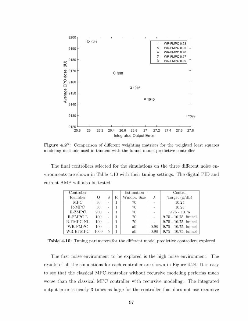
Integrated Output Error25.8 26 26.2 26.4 26.6 26.8 27 27.2 27.4 27.6 27.8
Ave
rage
EP
O d
ose,
(IU
)
9120
9130
9140
9150
9160
9170
9180
9190
9200
1099
1040
1016
998
981 WR-FMPC 0.93WR-FMPC 0.95WR-FMPC 0.96WR-FMPC 0.97WR-FMPC 0.99
Figure 4.27: Comparison of different weighting matrices for the weighted least squaresmodeling methods used in tandem with the funnel model predictive controller
The final controllers selected for the simulations on the three different noise en-
vironments are shown in Table 4.10 with their tuning settings. The digital PID and
current AMP will also be tested.
Controller Estimation ControlIdentifier Q S R Window Size λ Target (g/dL)
MPC 30 - 1 70 - 10.25R-MPC 30 - 1 70 - 10.25
R-ZMPC 200 - 1 70 - 9.75 - 10.75R-FMPC L 100 - 1 70 - 9.75 - 10.75, funnel
R-FMPC NL 100 - 1 70 - 9.75 - 10.75, funnelWR-FMPC 100 - 1 all 0.98 9.75 - 10.75, funnel
WR-EFMPC 1000 5 1 all 0.98 9.75 - 10.75, funnel
Table 4.10: Tuning parameters for the different model predictive controllers explored
The first noise environment to be explored is the high noise environment. The
results of all the simulations for each controller are shown in Figure 4.28. It is easy
to see that the classical MPC controller without recursive modeling performs much
worse than the classical MPC controller with recursive modeling. The integrated
output error is nearly 3 times as large for the controller that does not use recursive
97

modeling. The current AMP also performs very poorly in comparison to the rest of
control methods, having an integrated output error value 2 to 3 times larger than the
other controllers. The rest of the recursive and weighted recursive controllers per-
form relatively similar to each other in terms of state performance but some obvious
differences can be seen by comparing some of the controllers. When comparing the
recursive zone MPC controller with the static boundaries (R-ZMPC) to the linear C-
ARX recursive zone MPC controller with the funnel constraints (R-FMPC L), it can
be seen that the funnel constraints help to improve the state performance by 12.2%, as
well as reduce the total drug usage by 0.7%. This comes at the cost of more frequent
EPO dose changes, increasing the average change in EPO by 77.7%. The robustness
of the nonlinear C-ARX is not as good as the linear C-ARX method here. The non-
linear C-ARX method (R-FMPC NL) performs worse in state management (-16.1%)
and total drug usage (+1.1%) as compared to the linear version (R-FMPC L). The
weighted recursive zone MPC controller with the funnel constraints (WR-FMPC) of-
fers a slight improvement in the state management (+7.0%) over the non-weighted
version (R-FMPC L), but comes at the cost of slightly increased drug usage (+1.1%)
and controller aggressiveness (+5.5%). As expected, the weighted recursive least
squares economic zone MPC controller with the funnel constraints (WR-EFMPC)
performs slightly worse in state management (-5.1%) than the controller without the
economic term (WR-FMPC) but it reduces the total drug usage by approximately
2.7%. Another detriment of the economic term is the large increase in the controller
aggressiveness. It increases by 118% and is over the 1000 IU threshold that would be
desirable to stay beneath. Last but not least, the PID controller performs worse than
most of the MPC controllers in state management, but it also yields a lower total
drug usage. This feature of the PID controller is completely attributable to the fact
that when an acute disturbance occurs, the PID controller is sluggish to respond on
some patients as compared to the MPC controllers, which causes the PID controller
to give less dose for longer than the other controllers. The controller settings used for
the PID controller are easily able to handle all the patient models and disturbances
relatively well, with the least complex solution. The R-FMPC L and WR-FMPC
controller both have acceptable levels of controller aggressiveness and perform similar
here and would be the most desirable selection based on this noise criteria.
98
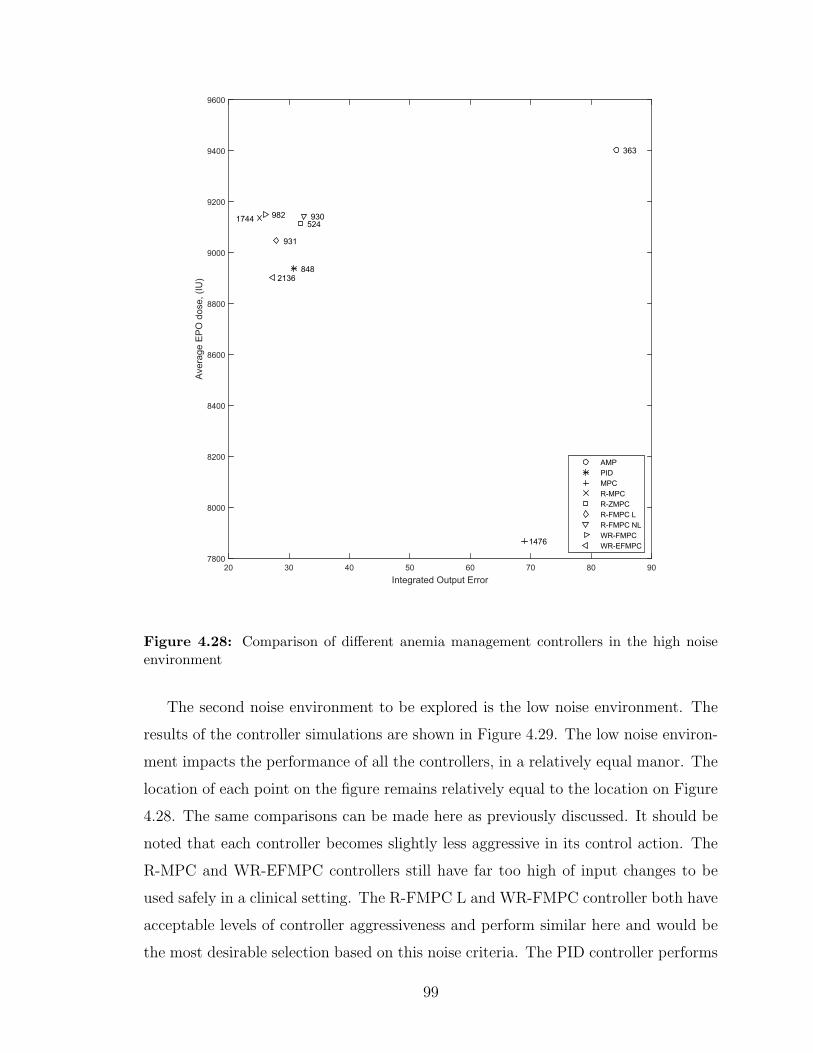
Integrated Output Error20 30 40 50 60 70 80 90
Ave
rage
EP
O d
ose,
(IU
)
7800
8000
8200
8400
8600
8800
9000
9200
9400
9600
363
848
1476
1744 524
931
930 982
2136
AMPPIDMPCR-MPCR-ZMPCR-FMPC LR-FMPC NLWR-FMPCWR-EFMPC
Figure 4.28: Comparison of different anemia management controllers in the high noiseenvironment
The second noise environment to be explored is the low noise environment. The
results of the controller simulations are shown in Figure 4.29. The low noise environ-
ment impacts the performance of all the controllers, in a relatively equal manor. The
location of each point on the figure remains relatively equal to the location on Figure
4.28. The same comparisons can be made here as previously discussed. It should be
noted that each controller becomes slightly less aggressive in its control action. The
R-MPC and WR-EFMPC controllers still have far too high of input changes to be
used safely in a clinical setting. The R-FMPC L and WR-FMPC controller both have
acceptable levels of controller aggressiveness and perform similar here and would be
the most desirable selection based on this noise criteria. The PID controller performs
99

fairly well, but again its sluggishness on acute disturbances is an undesirable feature.
Integrated Output Error20 30 40 50 60 70 80
Ave
rage
EP
O d
ose,
(IU
)
8000
8200
8400
8600
8800
9000
9200
9400
303
539
965
1436 447
783
756 810
1379
AMPPIDMPCR-MPCR-ZMPCR-FMPC LR-FMPC NLWR-FMPCWR-EFMPC
Figure 4.29: Comparison of different anemia management controllers in the low noiseenvironment
The final noise environment was used to perform controller simulations. This en-
vironment keeps the high measurement noise but does not use the integrating process
noise. This is not likely to occur in a clinical setting, but it is a good exploratory
exercise to see the impact that the integrating disturbance has on the controller per-
formance. The controller performance shifts quite a bit in comparison to the other
two noise environments. In these simulations, the classical MPC controller without
recursive modeling performs much better than previously, as expected. The R-ZMPC
controller has a similar state performance location relative to the others, but it comes
100

at the cost of much larger drug usage. This is the result of the hemoglobin set-
tling near the top of the control zone more often than the other controllers. These
simulations include only negative acute disturbances, which will cause the R-ZMPC
controller to settle near the top boundary more often as the controller forces the Hgb
upwards after the disturbance. The R-FMPC NL controller still performs worse as
compared to the linear version, which solidifies the linear modeling method as the
method of choice to obtain a C-ARX model. The aggressiveness of the WR-EFMPC
and R-MPC controller are still quite high, and taking into consideration the previous
results, these controllers are not recommended for use.
Integrated Output Error10 15 20 25 30 35 40 45 50
Ave
rage
EP
O d
ose
(IU)
8200
8400
8600
8800
9000
9200
9400
9600
220
486
814
1188
345
595
543 613
1189
AMPPIDMPCR-MPCR-ZMPCR-FMPC LR-FMPC NLWR-FMPCWR-EFMPC
Figure 4.30: Comparison of different anemia management controllers in the noise envi-ronment without the integrating disturbance
101

Several of the simulations, with a partial showing of the controllers, will be used
to illustrate abnormalities that are common with some of the controller methods.
The first two figures are shown in Figure 4.31. In figure (a), the AMP causes a lot of
oscillations in the hemoglobin. In figure (b), the current AMP is unable to provide
proper doses for this patient, which would necessitate the divergence from the current
AMP leaving the physician to choose doses for the patient blindly. In both cases, the
WR-FMPC controller is able to control the hemoglobin value well.
0 50 100 150 200 250 300 350 400 450 500
Hem
oglo
bin,
yk (g
/dL)
7
8
9
10
11
12
13
Time (weeks)0 50 100 150 200 250 300 350 400 450 500
EP
O D
ose,
uk (I
U)
×104
0
0.5
1
1.5
2
2.5
3
AMPWR-FMPC
(a) AMP induced Hgb Oscillation
0 50 100 150 200 250 300 350 400 450 500
Hem
oglo
bin,
yk (g
/dL)
7
8
9
10
11
12
13
Time (weeks)0 50 100 150 200 250 300 350 400 450 500
EP
O D
ose,
uk (I
U)
×104
0
0.5
1
1.5
2
2.5
3
AMPWR-FMPC
(b) Divergence from AMP necessary
Figure 4.31: Simulation Results where the current AMP fails to control the patient Hgbadequately
Figure 4.32a shows the importance of the recursive modeling algorithm. A com-
parison of classical MPC and R-MPC shows that without recursive modeling, the
MPC controller cannot account for changing patient health. Figure 4.32b shows the
tendency of the R-ZMPC controller to settle near the upper boundary in these simu-
lation tests. Due to the fact that all the acute disturbances are negative, the R-ZMPC
controller will often guide the hgb to the upper part of the control zone, which will
use more drug than necessary to maintain the hgb in the desired range. Less com-
monly, the reverse also happens, where the hgb settles near the bottom. It is not fair
to judge the R-ZMPC controller by its increased drug usage because of the different
control zone shape, but it highlights the fact that the hgb values will often be near the
boundaries of the zone, and small disturbances and noise can push the state outside
of the control zone more easily.
102

0 50 100 150 200 250 300 350 400 450 500
Hem
oglo
bin,
yk (g
/dL)
7
8
9
10
11
12
13
Time (weeks)0 50 100 150 200 250 300 350 400 450 500
EP
O D
ose,
uk (I
U)
×104
0
0.5
1
1.5
2
2.5
3
WR-FMPCMPCR-MPC
(a) MPC fails without recursive modeling
0 50 100 150 200 250 300 350 400 450 500
Hem
oglo
bin,
yk (g
/dL)
7
8
9
10
11
12
13
Time (weeks)0 50 100 150 200 250 300 350 400 450 500
EP
O D
ose,
uk (I
U)
×104
0
0.5
1
1.5
2
2.5
3
AMPR-ZMPCWR-FMPC
(b) Zone MPC using excessive EPO
Figure 4.32: Simulation Results showing the importance of recursive modeling, and a casewhere R-ZMPC uses much more drug dose than necessary
Figure 4.33 shows two cases which magnify the problem with the digital PID con-
troller, while showing the WR-FMPC controllers ability to handle the situations well.
Figure 4.33a shows the sluggishness of the PID controller during acute disturbances.
The PID controller is late to respond to a step disturbance, and overshoots the target
zone around the 375 week mark. The PID controller could be tuned individually to
better manage this patient, but it will be difficult to manage each patient individu-
ally. The WR-FMPC algorithm is a one-size-fits-all algorithm with identical tuning
settings for each patient.
0 50 100 150 200 250 300 350 400 450 500
Hem
oglo
bin,
yk (g
/dL)
7
8
9
10
11
12
13
Time (weeks)0 50 100 150 200 250 300 350 400 450 500
EP
O D
ose,
uk (I
U)
×104
0
0.5
1
1.5
2
2.5
3
PIDAMPWR-FMPC
(a) PID performs sluggishly
0 50 100 150 200 250 300 350 400 450 500
Hem
oglo
bin,
yk (g
/dL)
7
8
9
10
11
12
13
Time (weeks)0 50 100 150 200 250 300 350 400 450 500
EP
O D
ose,
uk (I
U)
×104
0
0.5
1
1.5
2
2.5
3
PIDAMPWR-FMPC
(b) MPC handles modeling without a dose
Figure 4.33: Simulation Results showing some of the failures of the PID controller
103

Figure 4.33b shows a case where no EPO dose is given for almost two years. The
WR-FMPC controller is still able to counter the acute disturbance at the 400 week
mark, due to the constrained modeling technique. The PID controller performs very
poorly here due to integral wind-up. The sluggishness of the PID controller can also
been seen again in this figure in the 175 to 225 week mark, where the PID responds
slowly to the disturbances and overshoots the target zone both times.
Figure 4.34 shows two cases where the patient health changes significantly over
the course of the simulation due to the integrating disturbance. The zone MPC
controllers with the funnel constraints are able to control both of these situations
well.
0 50 100 150 200 250 300 350 400 450 500
Hem
oglo
bin,
yk (g
/dL)
7
8
9
10
11
12
13
Time (weeks)0 50 100 150 200 250 300 350 400 450 500
EP
O D
ose,
uk (I
U)
×104
0
0.5
1
1.5
2
2.5
3
AMPR-FMPC LR-FMPC NLWR-FMPC
(a) Patient health changes drastically
0 50 100 150 200 250 300 350 400 450 500
Hem
oglo
bin,
yk (g
/dL)
7
8
9
10
11
12
13
Time (weeks)0 50 100 150 200 250 300 350 400 450 500
EP
O D
ose,
uk (I
U)
×104
0
0.5
1
1.5
2
2.5
3
AMPR-FMPC LR-FMPC NLWR-FMPC
(b) Patient health improves over time
Figure 4.34: Simulation Results showing some patients that have a decaying/improvinghealth over time
Figure 4.35 shows the difficulties in obtaining a one-size-fits-all set of tuning pa-
rameters for the patients for economic MPC (WR-EFMPC). Utilizing the economic
term can offer improvements in drug savings, but the controller is difficult to tune for
the whole set of patients and results in reduced ability to manage the state effectively.
The state management should not be sacrificed to reduce the cost of ESA treatment.
Figure 4.35a shows a case where the economic controller is very aggressive, while
Figure 4.35b shows a case with the same tuning settings where the controller is not
very aggressive. Both simulations show that the economic term usually just causes a
slight offset between WR-EFMPC and WR-FMPC.
104

0 50 100 150 200 250 300 350 400 450 500
Hem
oglo
bin,
yk (g
/dL)
7
8
9
10
11
12
13
Time (weeks)0 50 100 150 200 250 300 350 400 450 500
EP
O D
ose,
uk (I
U)
×104
0
0.5
1
1.5
2
2.5
3
AMPWR-FMPCWR-EFMPC
(a) Aggressiveness is high for this patient
0 50 100 150 200 250 300 350 400 450 500
Hem
oglo
bin,
yk (g
/dL)
7
8
9
10
11
12
13
Time (weeks)0 50 100 150 200 250 300 350 400 450 500
EP
O D
ose,
uk (I
U)
×104
0
0.5
1
1.5
2
2.5
3
AMPWR-FMPCWR-EFMPC
(b) Aggressiveness is low for this patient
Figure 4.35: Simulation Results showing the difficulty for obtaining a one-size-fits-all setof tuning parameters for economic R-FMPC
Figure 4.36a shows the reduced performance that the nonlinear C-ARX method
provides during control. The reduced performance might be attributed to the ro-
bustness of the fmincon function and its ability to find a proper model at each time
point. If no model is obtained, the previous model is used. The linear QP version
of the C-ARX method is far more robust than the NLP version, and it rarely ever
fails to find a minimum solution. The nonlinear method is not recommended for use
in the clinical setting. The controller decision comes down to a choice between the
linear weighted and non-weighted recursive zone MPC controllers with the funnel
constraints (WR-FMPC and R-FMPC). Figure 4.36b shows there is minimal differ-
ence between the weighted and non-weighted versions of R-FMPC. These results align
with the modeling results, as little difference is also seen between the two modeling
methods. As the state management lags slightly in the non-weighted version for all
three noise environments, the linear weighted recursive zone model predictive control
using the funnel constraints (WR-FMPC) is recommended for use.
105

0 50 100 150 200 250 300 350 400 450 500
Hem
oglo
bin,
yk (g
/dL)
7
8
9
10
11
12
13
Time (weeks)0 50 100 150 200 250 300 350 400 450 500
EP
O D
ose,
uk (I
U)
×104
0
0.5
1
1.5
2
2.5
3
R-FMPC LR-FMPC NLWR-FMPC
(a) Nonlinear modeling performs poorly
0 50 100 150 200 250 300 350 400 450 500
Hem
oglo
bin,
yk (g
/dL)
7
8
9
10
11
12
13
Time (weeks)0 50 100 150 200 250 300 350 400 450 500
EP
O D
ose,
uk (I
U)
×104
0
0.5
1
1.5
2
2.5
3
R-FMPC LWR-FMPC
(b) Minimal difference exhibited
Figure 4.36: Simulation Results showing the minimal difference between weighted andnon-weighted R-FMPC and the poor performance of the nonlinear C-ARX method forrecursive model estimation
4.4 Conclusion
In the simulations performed using the C-ARX models as the simulation patient,
the ZMPC controller with the funnel constraints had comparable state management
to that of the highest performing controllers utilizing chance constraint formulations.
The exception was that the ZMPC (funnel) controller also had a lower total drug
usage, as well as a far lower average rate of change as compared to the Chance Con-
strained controllers. Using the funnel constraint allows the tuning parameters to be
set to a one-size-fits-all configuration where the controller aggressively changes the
input only if the state exists outside of the zone, while remaining almost stationary, if
within the zone. Due to the large number of clinical patients, this tuning robustness
is a highly sought after feature of Zone MPC.
Due to the time-varying nature of the clinical patients and frequent disturbances
on the system, it is not enough to implement a controller without a method for updat-
ing the model. The simulation results using the PKPD model as the patient simulator,
along with the integrating process noise and random acute disturbances, tested the
controllers in the most rigorous of simulation tests. The integrating process noise
106
offers unique challenges to overcome because it is possible to have an accumulation of
the disturbance over time. The controller must be able to properly account for this
added disturbance. Due to modeling inaccuracies and modeling error using a linear
model on a nonlinear system, the process models used in the controller may produce
large offset and non-optimal solutions as the hemoglobin extends beyond the models
valid range. Recursively estimating a constrained ARX model at each sampling time
produces a highly robust controller to the time-varying nature of the process model.
It is important to restrict the model parameters to a particular structure to ensure
each model attained will be appropriate for use. Without restricting the structure,
it is difficult to know whether the optimal modeling solution will produce a model of
the system that will validate well. Without the constraints, the attained model may
also be unstable, which does not match theoretical expectations.
Many different types of controllers were tested through the use of computer simu-
lations. Observing the simulation results, it is recommended to implement a Weighted
Recursive Zone Model Predictive Controller utilizing the funnel control zone (WR-
FMPC), using a longer window size in the length of 70+ weeks. It is recommended
that the weighting in weighted least squares be a value of λ=0.98 or greater. The
data should also be filtered to remove some effects of the measurement noise. The
recommended filter is an EWMA filter as presented with a filter value α=0.75. The
funnel shape should be tuned according to the equations presented using a value of
p=0.6. The controller should have the cost function tuning weights set at Q=100 and
R=1. The prediction horizon should be set to N=8.
107

Chapter 5
Future Work
5.1 Introduction
This chapter outlines the future areas of research that have been identified to date.
5.1.1 Patient Simulator
Significant improvements can be made to the patient simulator. The current
simulator relies on a PKPD model estimated from data, random integrating and
measurement noise and step and ramp disturbances. A wiser choice would be to
build the patient simulator solely based on measurement noise and time-varying pa-
rameters in the PKPD model. The disturbances and changes in patient health could
then be explained by biological mechanisms, rather than random noise. One of the
current uncertainties in the controller performance assessment on the current patient
simulator design is that the PKPD model never changes. Therefore, the system gain
remains static. In actuality, the system gain would be time-varying and dependent on
ever-changing model parameters. The current simulator design may give misleading
controller performance results as a result of the static gain.
An efficient patient simulator is needed that is able to more accurately reflect the
behaviour of an actual patient. It may be necessary to have government approval
of the patient simulator to allow the controller performance simulation results to act
as an acceptable pre-clinical trial. This order of events would be similar to what
exists for Type 1 Diabetes. The UVA PADOVA Type 1 Diabetes Simulator exists
as an FDA approved simulator in the USA (C. Man, 2014), and is sufficient to test
controllers on for pre-clinical trials.
108

5.1.2 Process Model Improvement
The foundation of any model predictive controller is the system model. A great
deal of time has been spent perfecting the constrained ARX modeling method but
the model structure may be able to be improved. A more complex model involving
more hemoglobin measurements or a disturbance model may offer an improved model.
Using additional inputs or outputs such as iron doses, iron levels or white blood cell
counts may offer modeling improvements. Different model types, such as a neural
network may also provide improved modeling results, resulting in better controller
performance.
5.1.3 Advanced Model Predictive Controllers using Param-eter Uncertainty
The stochastic controllers in this work included only additive process noise as the
uncertainty. A more appropriate controller would include parameter uncertainty in
the controller formulation. It is possible that the inclusion of parameter uncertainty
or different forms of robust optimization may offer improved control results.
5.1.4 Self-tuning PID
The Digital PID controller presented in this thesis was designed empirically using
many simulations performed on several different patient models. Its performance was
not perfected as opposed to that of the model predictive controllers. Given the good
performance seen by the PID controller on most models, a self-tuning PID controller
may be able to overcome the issues seen on a small fraction of the patients, as well
as improve the performance in general.
109

Bibliography
A. Gaweda, A. Jacobs, G. Aronoff M. Brier (2008). Model predictive control of ery-
thropoietin administration in the anemia of esrd. Am J Kidney Dis 51, 71–79.
A. Gaweda, A. Jacobs, G. Aronoff S. Rai M. Brier (2014). Individualized anemia
management reduces hemoglobin variability in hemodialysis patients. Journal of
the American Society of Nephrology 25, 159–166.
A. Gaweda, M. Brier, A. Jacobs G. Aronoff B. Nathanson M. Germain (2010). De-
termining optimum hemoglobin sampling for anemia management from every-
treatment data. Clinical Journal of the American Society of Nephrology 5, 1939–
1945.
A. Levey, R. Atkins, J. Coresh (2007). Chronic kidney disease as a global public
health problem: approaches and initiatives - a position statement from kidney
disease improving global outcomes. Kidney International 72, 247–259.
A. Parisio, M. Molinari, D. Varagnolo K. Johansson (2013). A scenario-based predic-
tive control approach to building hvac management systems. IEEE International
Conference on Automation Science pp. 428–435.
Allgower, F., R. Findeisen and Z. Nagy (2004). Nonlinear model predictive control:
From theory to application. Journal of the Chinese Institute of Chemical Engi-
neers 35, 299–315.
B. Grosman, E. Dassau, H. Zisser L. Jovanovic F. Doyle (2010). Zone model predictive
control: A strategy to minimize hyper- and hypoglycemic events. Journal of
Diabetes Science and Technology 4, 961–975.
110
Bemporady, A., L. Pugliay and T. Gabbriellin (2011). A stochastic model predictive
control approach to dynamic option hedging with transaction costs. In: American
Control Conference. O’Farrell Street, San Francisco, CA, USA. pp. 3862–3867.
Bogacki, P. and L. Shampine (1989). A 3(2) pair of runge - kutta formulas. Applied
Mathematics 4, 321–325.
C. Man, F. Micheletto, D. Lv M. Breton B. Kovatchev C. Cobelli (2014). The
uva/padova type 1 diabetes simulator: New features. Journal of Diabetes and
Technology 8, 26–34.
Chait, Y., J. Horowitz, B. Nichols, R. Shrestha and M. Germain C. Hollot (2014).
Control-relevant erythropoiesis modeling in end-stage renal disease. IEEE Trans-
actions on Biomedical Engineering 61, 658–664.
Christopher, P. (2000). Designing efficient software for solving delay differential equa-
tions. Journal of Computational and Applied Mathematics 125, 287–295.
Damien, P., H. Lanham, M. Parthasarathy and N. Shah (2016). Assessing key cost
drivers associated with caring for chronic kidney disease patients. BioMed Central
Health Services Research.
Elliot, S. (2008). Erythropoiesis-stimulating agents and other methods to enhance
oxygen transport. British Journal of Pharmacology 154, 529–541.
Gondhalekar, R., E. Dassau, H. Zisser and F. Doyle III (2013). Periodic-zone model
predictive control for diurnal closed-loop operation of an artificial pancreas. Jour-
nal of Diabetes Science and Technology 7, 1446–1460.
Grosso, J., C. Ocamp-Martinex, V. Puig and B. Joseph (2014). Chance-constrained
model predictive control for drinking waternetworks. Journal of Process Control
24, 504–516.
J. Garriga, M. Soroush (2010). Model predictive control tuning methods: A review.
Ind. Eng. Chem. Res 49, 3505–3515.
111

J. Rawlings, K. Muske (1993). Model predictive control with linear models. AIChE
Journal 39, 262–287.
Jing, Z., Y. Wei-jie, Z. Nan, Z. Yi and W. Ling (2012). Hemoglobin targets for chronic
kidney disease patients with anemia: A systematic review and meta-analysis.
Journal of American Institue of Chemical Engineers 7, 1–9.
Knab, T., G. Clermont and R. Parker (2015). Zone model predictive control and
moving horizon estimation for the regulation of blood glucose in critical care
patients. In: Proceedings of The 9th International Symposium on Advanced Con-
trol of Chemical Processes, The International Federation of Automatic Control.
Whistler, British Columbia, Canada.
M. Brier, A. Gaweda, A. Dailey A. Jacobs G. Aronoff (2010). Randomized trial of
model predictive control for improved anemia management. Clinical Journal of
the American Society of Nephrology 5, 814–820.
National Kidney Foundation, NKF (2017). Global facts: About kidney disease.
https://www.kidney.org, accessed June 2017.
O’Dwyer, A. (2006). Handobok of PI and PID Controller Tuning Rules. Imperial
College Press.
Pannocchia, G. and J. Rawlings (2003). Disturbance models for offset-free model-
predictive control. Journal of the American Institute of Chemical Engineering
49, 426–437.
Park, I., S. Ahn, Y. Kim, S. Kang and S. Cho (2014). Performance evaluation of
samsung labgeo hc10 hematology analyzer. Archives of Pathology & Laboratory
Medicine.
Rawlings, J. (2000). Tutorial overview of model predictive control. IEEE Control
Systems pp. 38–52.
Ren, J., J. McAllister, Z. Li, J. Liu and U. Simonsmeier (2017). Modeling of
hemoglobin response to erythropoietin therapy through contrained optimization.
112

In: Proceedings of The 6th International Symposium on Advanced Control of In-
dustrial Processes. Taipei, Taiwan.
Rockafellar, R. and S. Uryasev (2000). Optimization of conditional value-at-risk. Jour-
nal of Risk 2, 21–42.
Rosner, M. and W. Bolton (2008). The mortality risk associated with higher
hemoglobin: Is therapy to blame?. Kidney International 74, 782–791.
S. Trevitt, S. Simpson, A. Wood (2016). Articial pancreas device systems for the
closed-loop control of type 1 diabetes: What systems are in development?. Jour-
nal of Diabetes Science and Technology 10, 714–723.
Seborg, D., T. Edgar, D. Mellichamp and F. Doyle (2011). Process Dynamics and
Control. John Wiley and Sons Inc.
Shampine, L. (2004). Error estimation and contol for odes.
Shampine, L. and S. Thompson (2001). Solving ddes in matlab. Applied Numerical
Mathematics 37, 441–458.
Singh, A. (2007). The target hemoglobin level in patients on dialysis. Dialysis and
Transplantation 36, 1–3.
Singh, A., L. Szczech, K. Tang, H. Barnhart, S. Sapp, M. Wolfson and D. Reddan
(2006). Correction of anemia with epoetin alfa in chronic kidney disease. New
England Journal of Medicine 355, 2085–2098.
Soderstrom, T. and P. Stoica (1989). System Identification. Prentice Halll.
Turksoy, K., L. Quinn, E. Littlejohn and A. Cinar (2014). Multivariable adaptive
identification and control for artificial pancreas systems. IEEE Transactions on
Biomedical Engineering 61, 883–891.
V. Batora, M. Tarnik, J. Murgas, S. Schmidt, K. Norgaard, N. Poulsen, H. Madsen,
D. Boiroux and J. Jorgensen (2015). The contribution of glucagon in an artificial
pancreas for people with type 1 diabetes. In: Proceedings of the American Control
Conference. Chicago, Illinois, USA. pp. 5097–5102.
113

V. Bobal, J. Bohm, J. Fessl J. Machacek (2005). Digital Self Tuning Controllers.
Springer-Verlag London Ltd.
V. Jha, G. Garcia-Garcia, K. Iseki (2013). Chronic kideny disease: Global dimension
and perspectives. Lancet 382, 260–272.
W. Couser, G. Remuzzi, S. Mendis M. Tonelli (2011). The contribution of chronic
kidney disease to the global burden of major noncommunicable diseases. Kidney
International 80, 1258–1270.
114