Co-control of Urban Air Pollutants and Greenhouse Gases in Mexico City

J. Jason West, Patricia Osnaya, Israel Laguna, Julia Martínez, and Adrián Fernández

Instituto Nacional de Ecología, México

February, 2003

Completed with support from the Integrated Environmental Strategies Program of the US National Renewable Energy Laboratory and the

US Environmental Protection Agency

2

Table of Contents Executive Summary Resumen Ejecutivo (Executive Summary in Spanish) Acknowledgments Chapter 1 – Introduction, Motivation, and Goals for Analyzing the Co-Control of Urban

Air Pollutants and Greenhouse Gases in Mexico City Chapter 2 – Creating a Harmonized Database of Emissions Control Options for Mexico

City Chapter 3 – Initial Exploration of Synergies and Tradeoffs Using the Harmonized Database

of Options Chapter 4 – Development of a Linear Programming Model for Analyzing Co-Control Chapter 5 – Analysis of the Co-Control of Urban Air Pollutants and Greenhouse Gases Chapter 6 – Development and Application of Goal Programming for Mexico City Chapter 7 – Conclusions and Recommendations References Appendix A – Calculation notes on the costs and emissions reductions of the local air

quality measures, and GHG measures from individual studies (in Spanish). Appendix B – Calculation notes on the costs and emissions reductions of the GHG

mitigation measures (in Spanish). Appendix C – User’s guide to the linear program developed in Microsoft Excel. Appendix D – Report on August, 2002 Co-control / Co-benefits workshop in Mexico City.

3

EXECUTIVE SUMMARY The problems of climate change and air pollution share many common sources, notably through the combustion of fossil fuels. These shared sources suggest that emissions reduction strategies can be pursued to address both problems simultaneously. In this study, we develop a framework that accounts for these synergies in developing a comprehensive plan for the “co-control” of greenhouse gases (GHGs) and urban air pollutants. This project was conducted at the Instituto Nacional de Ecología (National Institute of Ecology), in coordination with other institutions that form the Comisión Ambiental Metropolitana (CAM, Metropolitan Environmental Commission) – the Secretaría de Medio Ambiente del Distrito Federal (Secretariat of the Environment of the Federal District) and the Secretaría de Ecología del Gobierno del Estado de México (Secretariat of Ecology of the Government of the State of Mexico). The project was funded by the Integrated Environmental Strategies program of the US Environmental Protection Agency and the US National Renewable Energy Laboratory. The objective of this project is to build capacity in Mexico, particularly in the government, for addressing the problems of urban air pollution in Mexico City and global climate change in an integrated way. This overall objective is achieved by:

1) Unifying existing information on the costs and emissions reductions associated with different control strategies – PROAIRE (Program to Improve the Air Quality in the Metropolitan Area of the Valley of Mexico, 2002-2010) and separate studies focused on GHG mitigation – into one harmonized database of options for analyzing the joint management of urban air pollutants and GHGs in Mexico City.

2) Implementing decision-support tools – based on Linear Programming (LP) and

Goal Programming (GP) – that can be used to analyze least-cost strategies for meeting multiple targets for multiple pollutants simultaneously. In addition to using these tools for analyzing the relationship between controls on local air pollutants and GHGs, the objective is to create user-friendly tools and train members of government offices in their use.

In constructing the harmonized database of options, we conducted a process that was open to all institutions of the CAM. The estimates of costs and emissions reductions in PROAIRE were carefully reviewed, making important revisions that are fully documented. We estimated for the first time changes in CO2 emissions from the PROAIRE measures, changes in local air pollutant emissions from the GHG measures, and estimates of the total investment cost and net present value (NPV) in ways that are consistent for all measures. Here, the NPV indicator includes the investment cost, fuel expenditures, and the salvage value of the investment in 2010, omitting other changes in operation and maintenance costs. As uncertainties in the database of options are likely large, caution should be taken when using the database to evaluate individual measures, but that it can be used sensibly to investigate GHG and air pollutant control more broadly.

4

We estimate that if PROAIRE measures are implemented as planned, they will result in a significant “co-benefit” in a reduction of 3.1% of projected CO2 emissions in 2010, in addition to a substantial reduction in emissions of local pollutants. These CO2 reductions are distributed unevenly among measures, with some measures causing net CO2 increases. Overall, about half of the CO2 reductions derive from the adoption of new vehicles and half from measures to improve the transport infrastructure. Meanwhile, the GHG emissions reduction measures together are estimated to cause an 8.7% reduction of the projected 2010 CO2 emissions, but only modest reductions in emissions of local pollutants (3.2% HC, 1.4% NOX, and 1.3% PM10). The reductions in emissions of local pollutants are estimated to be small for the electricity efficiency measures because most of the electricity generated for Mexico City comes from outside of the metropolitan region – under other assumptions or in other locations, these reductions might be greater. Several of the GHG measures are also observed to have a negative NPV, coming at a net cost savings through the savings achieved in fuel expenditures, although these measures often require high investment costs. The LP is used in this study as an efficient search tool for finding the set of options that most cost-effectively meets targets for emissions reductions of multiple pollutants. While cost is clearly important for decisions, other important factors that may be difficult to quantify are not included in this study. When applying the LP to consider the case of achieving PROAIRE emissions reduction targets, using only the PROAIRE measures, we find that it is possible to reduce the overall cost of the program by about 20% (for both the total investment cost and the NPV), by adjusting investments towards the more cost-effective measures. Lower cost solutions are not possible using this dataset because PROAIRE is an ambitious air quality plan, proposing to implement measures near the maximum extent feasible. When allowing investments in the GHG measures, we find that the minimum investment solution shows little change, but a significantly lower NPV can be achieved through investments in GHG measures, with a significant reduction in CO2 emissions. This low NPV solution suggests that the GHG (efficiency) measures can be included as part of an urban air quality plan because of their net cost-saving potential, even if the local emissions reductions from these measures may be modest. The LP is applied to consider the co-control goals by forcing the local PROAIRE emissions reduction goals to be met, while adding constraints on the CO2 emissions. Additional CO2 emissions reductions are achieved most cost-effectively by investing in GHG mitigation measures, generally, rather than adjusting investments among the PROAIRE measures. Increasing the CO2 reduction target increases the total investment cost, but significantly decreases the NPV, as GHG measures with a negative NPV are generally selected as most cost-effective. This suggests that in the case of Mexico City, using the database of measures developed here, there is rather little synergy between local air pollution and climate change goals – the benefits of planning to address local and global pollution simultaneously are observed to be small, but they are not zero. If we allow for CO2 emissions reductions to be purchased outside of the metropolitan area, we find that there is potentially a large reservoir of CO2 reductions available elsewhere in Mexico. In one case, the most cost-effective plan is to invest in PROAIRE measures to

5

achieve local emissions reductions, and to purchase additional CO2 reductions only through forestry projects. This illustrates that, because the location of long-lived GHG emissions does not matter for climate, it is important to consider other opportunities for GHG emissions control in other sectors or geographic regions, which may not be the focus of a policy analysis. The LP was further used to demonstrate that planning to achieve mitigation goals for urban air pollutants and GHGs simultaneously is more cost-effective than planning separately, due to the “secondary” benefits of each type of measure, although the benefit of this simultaneous planning is estimated to be small. For policy, therefore, the main risk in planning separately may be in not recognizing these emissions reduction benefits. In addition to applying the LP, the GP was demonstrated to be useful in finding an emissions reduction plan that weighs multiple goals, rather than optimizing only for cost. We encourage Mexican government offices to continue to develop the GP so that the different goals and the weights applied to them reflect the priorities of decision-makers. The results of this study often indicate that the benefits of simultaneously planning urban air pollutant and GHG mitigation are small, as additional CO2 constraints are often met by investing in measures which target CO2, with modest changes in emissions of local pollutants. We caution however, that results may be different under different assumptions for Mexico City, or in other regions which differ geographically and technologically – in the case of Mexico City, the fact that little of the electricity is generated locally had an important impact on the findings. For the international co-benefits research community, this study has demonstrated that while some measures may have significant co-benefits for reducing emissions of both local and global pollutants, the best strategy to meet co-control goals may come from other combinations of local and global measures. Comprehensive planning to address both problems should start by compiling many emissions reduction options, including more than one emissions sector, and for GHG emissions, can include a larger geographical scope. The co-control approach and methods employed in this study should be used as a methodological addition to the methods used in co-benefits studies in the past.

6

RESUMEN EJECUTIVO Los problemas del cambio climático y la contaminación del aire son generados por diversas fuentes comunes, particularmente por la quema de combustibles fósiles. Lo anterior sugiere que se pueden desarrollar estrategias para la reducción de emisiones, las cuales pueden resolver ambos problemas simultáneamente. En el presente estudio, se desarrolla una metodología de análisis que incluye las sinergias para el desarrollo de un plan integral para el “control conjunto” (co-control) de las emisiones de gases de efecto invernadero (GEI) y contaminantes del aire urbano. El presente proyecto fue coordinado por el Instituto Nacional de Ecología, en colaboración con las otras instituciones que integran la Comisión Ambiental Metropolitana (CAM) – la Secretaría de Medio Ambiente del Distrito Federal y la Secretaría de Ecología del Gobierno del Estado de México. El proyecto fue financiado por el programa de Estrategias Ambientales Integradas (Integrated Environmental Strategies Program) de la Agencia de Protección Ambiental de los EUA (US Environmental Protection Agency), y del Laboratorio Nacional de Energía Renovable de los EUA (US National Renewable Energy Laboratory). El objetivo de este proyecto es apoyar el fortalecimiento institucional en México, particularmente en el gobierno, para la gestión de los problemas de la contaminación del aire en la ciudad de México y el cambio climático de manera integrada. Para cumplir con este objetivo se realizaron las siguientes actividades:

1) La unificación de la información existente sobre los costos y las reducciones de las emisiones asociadas a las diferentes estrategias de control – PROAIRE (Programa para Mejorar la Calidad del Aire en la Zona Metropolitana del Valle de México 2002-2010) y estudios enfocados en la mitigación de GEI – en una base de datos armonizada para el análisis de la gestión integrada de contaminantes urbanos del aire y de GEI en la ciudad de México.

2) La instrumentación de herramientas para el apoyo en la toma de decisiones –

basadas en los modelos: Programación Lineal (LP) y el “Goal Programming” (GP) – los cuales se utilizan para analizar estrategias que satisfacen objetivos para la disminución de contaminantes múltiples de manera simultánea. Adicionalmente al uso de estas herramientas para el análisis de las relaciones entre las medidas para la reducción de contaminantes locales del aire y los GEI, el objetivo es crear las que sean amigables al usuario, y aumentar la capacidad técnica de algunos integrantes de las instituciones del gobierno.

La construcción de la base de datos armonizada de las medidas se realizó a través de un proceso abierto a la participación de todas las instituciones de la CAM. Se revisaron con cuidado las estimaciones de los costos y de las reducciones de emisiones informadas en el PROAIRE. Dichas revisiones importantes están documentadas completamente. Se estimaron por primera vez los cambios en emisiones de CO2 de las medidas del PROAIRE, los cambios en las emisiones de contaminantes locales del aire de las medidas de GEI, y las estimaciones del costo total de las inversiones y del valor presente neto (VPN), de manera

7

que sean consistentes para todas las medidas. En este estudio, el indicador VPN incluye el costo de inversión, los gastos por el consumo de combustible, y el valor de recuperación en el año 2010, y no considera otros cambios en gastos por operación y mantenimiento. Dado que la incertidumbre en la base de datos de las medidas probablemente es grande, se sugiere tener cuidado en el uso de ésta para evaluar directamente medidas individuales. Dicha base de datos se puede utilizar razonablemente bien para analizar el control conjunto de GEI y contaminantes del aire a nivel más general. Se estima que si las medidas del PROAIRE se instrumentaran como está planificado, se obtendría como beneficio adicional significativo una reducción del 3.1% respecto de las emisiones de CO2 proyectadas en 2010, así como una disminución importante de emisiones de contaminantes locales. Estas reducciones de CO2 están distribuidas de manera desigual entre las medidas, con algunas que causan un incremento neto de CO2. En total, cerca de la mitad de las reducciones de CO2 se originan del uso de vehículos nuevos, y la otra mitad de las medidas para mejorar la infraestructura de transporte. Por otro lado, se calculó que las medidas para mitigar las emisiones de GEI reducen el 8.7% de las emisiones de CO2 proyectadas en total, pero se obtiene una reducción menor de emisiones de contaminantes locales (3.2% HC, 1.4% NOX, y 1.3% PM10). Se estima que las reducciones de dichos contaminantes locales serán pequeñas en el caso de las medidas de eficiencia eléctrica, dado que la mayor parte de la electricidad generada para el consumo de la ciudad de México proviene de afuera de la zona metropolitana – bajo otros supuestos o lugares, las reducciones pueden ser mayores. Se observó también que muchas de las medidas de GEI tienen un VPN negativo, lo cual indica que hay un ahorro neto de dinero debido a la disminución de los gastos para combustibles, aunque dichas medidas requieren comúnmente de costos elevados de inversión. El modelo LP se usa en este estudio como una herramienta para buscar la combinación de medidas que logren las metas de reducción de emisiones de múltiples contaminantes con la mayor costo-efectividad. Mientras que queda claro que el costo es importante para la toma de decisiones, en este estudio no se incluyeron otros factores importantes, los cuales pueden ser difíciles de cuantificar. Cuando se aplica el modelo LP para considerar el caso del logro de las metas de la reducción de emisiones del PROAIRE, utilizando sólo las medidas de éste, se encuentra que es posible reducir en un 20% el costo total del programa (para el costo de la inversión total y para el VPN), si se dirigen las inversiones hacia las medidas que son más costo-efectivas. Al utilizar esta base de datos, las soluciones de menor costo no son posibles, ya que PROAIRE es un plan ambicioso para mejorar la calidad del aire, que propone instrumentar las medidas cerca del nivel máximo factible. Al considerar que se permitan inversiones en las medidas de reducción de GEI, la solución de inversión mínima no cambia significativamente, pero se puede tener un VPN bastante menor por dicha inversión, con una reducción importante de emisiones de CO2. Esta solución de menor VPN sugiere que las medidas de GEI (de eficiencia) pueden formar parte del plan de calidad del aire urbano, dado su potencial de ahorro en el costo, aunque las reducciones en emisiones locales de dichas medidas no sean grandes.

8

Se aplica el modelo LP para considerar las metas de co-control y garantizar la realización de las metas de las reducciones de emisiones locales del PROAIRE, mientras que se añaden restricciones en las emisiones de CO2. Las reducciones adicionales de emisiones de CO2 se alcanzan de manera más costo-efectiva por la inversión en medidas de mitigación de GEI, generalmente, en lugar de ajustar las inversiones entre las medidas del PROAIRE. Cuando se aumentan las metas de reducción de emisiones de CO2, el costo total de la inversión se incrementa y disminuye significativamente el VPN, ya que las medidas de disminución de GEI, con un VPN negativo, son seleccionadas generalmente como las más costo-efectivas. Esto sugiere que en el caso de la ciudad de México, al utilizar la base de datos desarrollada en el presente estudio, existe una sinergia poco importante entre las metas para mejorar la calidad del aire local y para el cambio climático – se observa que los beneficios de la planificación integrada para lograr metas simultáneas en la contaminación local y global son pequeños, pero no son cero. Se estima que hay un gran potencial de reducción de emisiones CO2 en el resto del país, como para que se llevara a cabo la compra de éstos mediante proyectos fuera de la zona metropolitana. En caso dado, el plan más costo-efectivo sería invertir en medidas del PROAIRE para alcanzar reducciones de emisiones locales, y comprar reducciones de CO2 adicionales únicamente mediante proyectos forestales. Eso ilustra que para el cambio climático no importa donde se reduzcan las emisiones GEI de larga vida y que es importante considerar otras oportunidades para el control de éstas en otros sectores o regiones geográficas, las cuales podrían no ser el punto central del análisis de políticas. También se utilizó el modelo LP para demostrar que planificar para lograr metas simultáneas de mitigación de contaminantes urbanos del aire y de GEI es más costo-efectivo que separadas, debido a los beneficios “secundarios” de cada tipo de medida, aunque se estima que los beneficios de la planificación simultánea serán pequeños. Para la elaboración de políticas, por lo tanto, el mayor riesgo de la planificación separada puede ser el no reconocer los beneficios de la reducción de emisiones. Adicional a la aplicación del modelo LP, en el estudio se muestra que el modelo GP es útil para encontrar un plan de reducción de emisiones que sopese metas múltiples, en lugar de optimizar sólo por el costo. Se aconseja que las instituciones del gobierno mexicano continúen el desarrollo de éste último, para que las diferentes metas, con la importancia que se le asigne a cada una, reflejen las prioridades de los tomadores de decisiones. Los resultados del presente estudio indican, de manera frecuente, que los beneficios de la planificación simultánea para la mitigación de contaminantes del aire y de GEI son pequeños, ya que a menudo se presentan restricciones adicionales por invertir en medidas enfocadas a reducir emisiones de CO2, con cambios pequeños en las emisiones de contaminantes locales. Sin embargo, es necesario tener cuidado ya que estos resultados pueden cambiar si se consideran diferentes condiciones para la cuidad de México, o en otras regiones que sean desiguales desde el punto de vista geográfico ó tecnológico – en el caso de la ciudad de México, el hecho de que poca electricidad se genere localmente tiene un efecto importante en los resultados.

9

Para la comunidad internacional que realiza investigaciones sobre co-beneficios, el presente estudio demuestra que aunque algunas medidas pudieran tener beneficios adicionales importantes, en la reducción de emisiones de contaminantes tanto locales como globales, la estrategia más efectiva para lograr metas de control conjunto puede provenir de otras combinaciones de medidas locales y globales. La planificación integral para enfrentar ambos problemas debe iniciar con la recopilación de muchas opciones para la reducción de emisiones, incluyendo más de un sector; y para las emisiones de GEI, se podría considerar una región geográfica más amplia. El enfoque de este tipo de control y los métodos empleados en este estudio deben utilizarse como un complemento a los métodos de estudios existentes.

10

Acknowledgments We are grateful for the financial support for this project received from the Integrated Environmental Strategies program of the US Environmental Protection Agency and the US National Renewable Energy Laboratory, under NREL subcontract number ADC-2-32409-01. Experts from the EPA and NREL contributed to the development of all aspects of this project, particularly in defining the project scope and goals. We are grateful for the contributions of J. Renné, C. Green, and D. Kline of NREL, and J. Leggett, S. Laitner, K. Sibold, S. Brant, L. Sperling, B. Hemming, M. Heil, and P. Schwengels of the EPA. In Mexico, this project benefited from discussions with many Mexican experts and researchers, both regarding the scope of the project, and the construction of the harmonized database of measures. At INE, we benefited from the contributions of INE staff V. Garibay, H. Martínez, P. Franco, A. Guzmán, A García, and visiting researchers H. Wornschimmel, S. Pulver, G. McKinley, and M. Zuk. We worked closely with members of other offices of the Comisión Ambiental Metropolitana (Metropolitan Environmental Commission), and we thank the following for their time and thoughtful contributions: V. H. Páramo, O. Vázquez, J. Sarmiento, C. Reyna, R. Reyes, R. Perrusquía, B. Valdez, M. Flores, B. Gutiérrez, J. Escandón, O. Higuera, and S. Victoria. Apart from government offices, we are grateful for the contributions we received from M. Hojer (consultant to World Bank), R. Favela (PEMEX), O. Masera (UNAM), W. Vergara (World Bank), J. A. Lopez-Silva (World Bank), J. Gasca (IMP), G. Sosa (IMP), J. Quintanilla (UMAM), F. Manzini (UNAM), A. Sierra (GM), P. Amar (NESCAUM), S. Connors (MIT), S. Vijay (MIT), J. Reilly (MIT), M. Sarofim (MIT). Finally we would like to thank and acknowledge A. Fernández for serving as host and advisor for this project. The friendship and hospitality shown by Dr. Fernández and all of his staff at INE was important to the success of this project, and will continue to pave the way for friendly and meaningful relationships between the US and Mexico for years to come.

Instituto Nacional de Ecología 5000 Periferico Sur

Col. Insurgentes Cuicuilco Del. Coyoacán

Mexico, DF 04530 MEXICO

www.ine.gob.mx

11

Chapter 1

Introduction, Motivation, and Goals for Analyzing the Co-Control of Urban Air Pollutants and Greenhouse Gases in Mexico City

1.1 The context of air pollution control in Mexico City The Mexico City Metropolitan Area (MCMA) has among the worst air pollution in the world, which is believed to cause significant effects on human health. This problem of air pollution has been addressed with significant success through two important emissions control initiatives implemented in the 1990s. The Metropolitan Environmental Commission (CAM) has recently released its new set of policy measures for addressing local air quality from 2002-2010 (PROAIRE; CAM, 2002). This plan was developed and agreed upon by the member organizations of CAM – the Secretariat of the Environment of the State of Mexico (SMA-EM), the Secretariat of the Environment of the Federal District (SMA-DF), and the federal government, represented by the Secretariat of the Environment and Natural Resources (SEMARNAT) and the National Institute of Ecology (INE). This plan includes a number of specific policy and technological measures for reducing emissions of local criteria pollutants. While PROAIRE is a long-term policy initiative just begun, reviews are planned for every two years. During these reviews, authorities plan to assess the implementation of the measures included in PROAIRE, and to adjust the resources given to different policy measures (including potentially including measures that were previously not included) as more information becomes available. Because these measures will be reevaluated, informing the decisions made in the forthcoming two-year review of PROAIRE is therefore an important motivation for studying the air pollution and GHG co-benefits associated with control actions in Mexico City. Further, while quantitative estimates of costs and emissions reductions of the different measures appear in the PROAIRE document, it is not clear how these numbers were put to use in informing the evaluation of the different measures, to determine which would be emphasized or omitted from PROAIRE. Some decision-makers have suggested that the lack of objective and quantitative decision analysis of the different policy options was an important shortcoming of PROAIRE, and could be an important part of the two-year evaluation of the measures in PROAIRE. 1.2 The context of climate change in Mexico Mexico is not part of Annex I of the Kyoto Protocol, and as such has not accepted a binding target for the reduction of greenhouse gas (GHG) emissions. Nonetheless, Mexico has significant interest in studying both its vulnerability to climate change, and options for reducing its domestic emissions. Mexico has fulfilled its obligations to the United Nations Framework Convention on Climate Change (UNFCCC) in part by submitting two national communications to the UNFCCC (SEMARNAT and INE, 2001), which include a national

12

emissions inventory of GHGs, an assessment of Mexico’s vulnerability to climate change, and prospects for GHG emissions reductions within Mexico’s borders. Mexico’s interest in GHG emissions reductions comes in part from the possibility that Annex I nations of the Kyoto Protocol, as well as other nations, could invest in GHG emissions reductions projects in less industrialized nations and claim the emissions reductions credit. As one of the more developed of the non-Annex I nations, Mexico is well-positioned to receive such investments in GHG emissions reductions projects. As the recipient of such investments, Mexico would want to make sure that such investments bring significant local benefits. One important way that Mexico could benefit is if the GHG emissions reductions projects also reduce emissions of local air pollutants, particularly in Mexico City, where air pollution is an acute problem. PROAIRE includes an emissions inventory of GHGs in the MCMA, but does not estimate the GHG emissions implications of the measures in PROAIRE, nor are any of the PROAIRE measures motivated to reduce GHG emissions. In fact, few government actions in Mexico, beyond pilot projects, have yet been authorized which have as a primary goal to reduce GHG emissions. Several studies of the costs and feasibility of actions to reduce greenhouse gases have been conducted in Mexico. But these studies have often said little about concurrent local benefits gained from reduced air pollution. The research conducted to date on the prospects for reducing GHG emissions and on evaluating local air quality control plans, have therefore been separate to a significant extent. 1.3 The context of international co-benefits research A number of interesting links exist between the problems of air pollution and climate change. These include scientific links, such as the fact that tropospheric ozone is both a criteria pollutant that causes health and environmental damage, and is a GHG which contributes to climate change. Within the last decade, the policy linkages between these two problems have been stressed, recognizing that since urban air pollutants and GHGs most commonly derive from the same sources – the combustion of fossil fuels – there is therefore the opportunity to address the two problems at the same time. From this recognition, the international co-benefits community has arisen to analyze the policy linkages between these problems. The approach most commonly taken in these studies has been to ask the question: if we take actions to reduce emissions of GHGs, what is the concurrent local benefit realized in terms of reduced air pollution and improved human health (Ekins, 1996; WGPHFC, 1997; Burtraw and Toman, 1997; NREL, 2000; Cifuentes et al., 2001)? These studies, conducted in several nations and urban areas around the world, have indeed found that the “secondary benefits,” “ancillary benefits,” or “co-benefits” of GHG mitigation are substantial, and can therefore provide supporting motivation for mitigating GHG emissions. This co-benefits research as it has been typically framed has given a position of primacy to the GHG emissions reductions, while effects on urban air pollutants are seen as the secondary benefits. In contrast to this approach, we can see that in Mexico City, and in many places, urban air pollution is what has effectively motivated emissions control

13

activities historically. Further, from an analytical point of view, co-benefits studies have failed to consider other means by which urban air pollutant emissions could be reduced – a GHG mitigation measure might be estimated to have large co-benefits for human health, but applying this measure may not be the best way to achieve the dual goals of reducing emissions of urban air pollutants and GHGs. Instead, it might be better to pursue different measures for GHG mitigation and for urban air pollution control. 1.4 Objectives and approach of this study In response to the co-benefits methods previously used, this work aims to approach the problem in a different way, viewing GHG emissions reductions in the context of ongoing efforts to control urban air pollution. More broadly, we propose to consider how emissions control plans can be constructed, which efficiently and effectively allow the multiple objectives of urban air pollution control and GHG mitigation to be achieved. In doing so, we will focus on the “control” side of the problem, and not on the “benefits” side. For that reason, we term this a project in “co-control” and present the methods used in this study as ones which are complementary to the “co-benefits” methods currently used. The Integrated Environmental Strategies (IES) project of the National Renewable Energy Laboratory (NREL) and the Environmental Protection Agency (EPA) of the United States, has stated its goals as being “to support and promote the analysis of public health and environmental benefits of integrated strategies for greenhouse gas mitigation and local environmental improvement in developing countries.” Consistent with the overall goals of IES, the objective of this project is to build capacity in Mexico, particularly in the CAM, for addressing the problems of urban air pollution in Mexico City and global climate change in an integrated way. This overall objective will be completed by fulfilling these objectives:

1) To unify existing information on the costs and emissions reductions associated with different control strategies – strategies proposed either for local air pollution control or for control of greenhouse gases – into one body of control actions. This harmonized database of options will form the foundation for analyzing the joint management of urban and global air pollution in Mexico City.

2) To implement decision-support tools – based on Linear Programming (LP) and Goal Programming (GP) – that can be used to analyze least-cost strategies for meeting multiple targets for multiple pollutants simultaneously. In addition to using these tools for analyzing the relationship between controls on local air pollutants and GHGs, the objective is to create a user-friendly model and train members of CAM in its use, so that it will be used in the future to inform decisions.

In completing these objectives we hope to fulfill multiple other objectives for different target audiences. For CAM, we expect that the quantitative decision support tools developed and employed in this study will be useful in informing urban air pollution control decisions, answering the need for objective methods to be used in policy analysis. We likewise expect that by presenting and analyzing GHG mitigation together with urban

14

air pollution control, we will promote the consideration of GHG mitigation in urban air quality planning and will advance the understanding of how these objectives are interrelated. For the community in Mexico studying and formulating policy on climate change, we expect this study to be useful in putting GHG mitigation in the context of urban air pollution control, and giving a framework for analyzing how the two goals can be pursued jointly. Likewise, this study should advance understanding of the local benefits to be gained from actions to decrease GHG emissions. Finally, for an international audience interested in co-benefits and emissions reductions potential in Mexico, this project will develop co-control methods which are complementary to the co-benefits methods currently used. We will further consider the extent to which goals of urban air pollution control and GHG mitigation are interrelated, synergistic, or competing – if we find, for example, that simultaneous planning for these two goals can reduce overall control costs substantially, then it suggests that this type of coordinated planning will be very important in achieving good policy solutions. 1.5 Tasks to fulfill objectives The first task to be completed is to create a coherent and self-consistent “harmonized” database of control measures, which combines emissions control measures from separate studies of urban air pollution control and GHG mitigation. In doing so, it is necessary to present all quantitative estimates for the measures under common assumptions, so that the different measures can be compared directly with one another. It is also necessary to estimate changes in emissions of GHGs due to the urban air pollution control measures, and to estimate changes in emissions of local air pollutants due to GHG mitigation measures. Finally, it is necessary to represent costs in common units for comparison. We focus on using information that already exists in Mexico in various studies, rather than making our own estimates of the costs and emissions reductions of different measures. One important outcome of this task will be to estimate for the first time the GHG emissions consequences of the PROAIRE measures. Second, it is necessary to construct the LP framework for analyzing the joint control of multiple pollutants simultaneously. Here the LP is a search tool, which we use to find the least-cost set of strategies for meeting targets on multiple pollutants at the same time. We choose to use an LP because it is especially useful when the control of more than two pollutants is considered, and can be an easily understood framework that CAM can continue to employ beyond the scope of this project. Likewise, the LP can be used reasonably as a basis for understanding how the preferred sets of policies (in this case, the least-cost set of policies) would change incrementally as emissions reduction objectives are varied. Because the LP can be used in this manner – for example, finding the incremental cost of GHG emissions control beyond urban air quality control, rather than on its own – we feel that the LP can be a very useful tool for this type of study.

15

Third, we will employ the LP model using the harmonized database of options, to explore the least-cost sets of emissions reduction strategies under a variety of constraints, which reflect questions relevant for CAM and for this project. Among these questions are:

- What is the most cost-effective set of options for meeting the emissions targets for local air pollutants given in PROAIRE?

- Could other measures not included in PROAIRE be part of a cost-effective solution to local air pollution?

- How does the total cost vary as local air pollutant emissions reduction targets are varied?

- What is the incremental cost of GHG emissions reductions beyond PROAIRE? - When adding a constraint on GHG emissions, are different control actions

preferred? - How do the control costs vary under different combinations of constraints on

emissions of local pollutants and GHGs? - What control options are robustly preferred under a variety of different

combinations of constraints? In applying the LP we focus on the cost-effectiveness of different control measures in constructing plans to meet objectives for meeting reductions of multiple pollutants simultaneously. In doing so, however, we caution that we are not trying in this study to state whether individual control actions are better others – we recognize the limitations of the dataset we are using and recognize that there are other important reasons for adopting or rejecting different policy measures, which are not reflected in this study. Nor are we trying to say that cost-effectiveness is the most important indicator that decision-makers should consider. Rather, we propose this method as a way of improving the quantitative policy analysis capabilities of CAM and of decision-makers in Mexico, that can become part of the planning process and part of the way decision-makers balance the diverse indicators and goals that they consider. Further, we propose these methods as a basis for us to consider experiments of varying different emissions targets, to try to learn broader lessons about what types of policies might be preferred under which combinations of targets. In addition to these specific research questions, we plan to use our database of measures and the LP to address a research hypothesis: that the overall cost of controlling simultaneously for local air pollutants and for GHGs, is less than the cost of controlling for these two goals individually. Stated differently, the hypothesis is:

Emissions reductions targets for local air quality and global climate can be achieved less expensively if planned simultaneously, than if they were planned separately:

Cost (Urban + Global) < Cost (Urban) + Cost (Global) The LP will be used to address whether, and to what degree, this hypothesis holds for the control actions considered in the MCMA, and whether the answer varies if different combinations of emissions constraints are chosen. If the cost of meeting targets simultaneously is significantly less, or if different control actions are favored, then this

16

would give strong support for the need for policy-makers to address these problems together. Finally, our discussions with experts in decision analysis in the United States has suggested that goal programming – a method which is founded on linear programming, but which allows multiple goals to be pursued simultaneously, rather than a single objective function – could be more appropriate than the LP alone for use by CAM in designing a coordinated urban air quality and GHG mitigation plan. Chapter 6 of this report presents the development of a goal programming model and illustrates its implementation. We conclude this document by presenting the conclusions and recommendations drawn from these results, with the goals of both aiding decision-makers in Mexico, and of learning more broadly about the relationships between the goals of urban air pollution control and GHG mitigation.

17

Chapter 2

Creating a Harmonized Database of Emissions Control Options for Mexico City In order to begin planning to control urban air pollutants and GHGs in a coordinated manner, it is necessary first to have a coherent database of options, which combines the options considered for urban air pollution control with those proposed for reduction of GHG emissions. Such a database of options should be consistent in its assumptions and metrics, so that different measures are directly comparable and can be evaluated in common terms. The goal of this chapter is to construct such a database of options using information already available for Mexico City. In doing so, we need to compile the different studies already conducted, estimate changes in emissions of GHGs for the measures proposed for the control of urban air pollutants, estimate the changes in emissions of urban air pollutants for the measures proposed for the control of GHG emissions, and ensure that costs are presented in common metrics. In this chapter, we first present the sources of information used in this study. We then present the methodological difficulties faced in resolving differences between these studies, and our methods of resolving these differences to create a coherent database of options. We then define the indicators of cost and emissions reductions that we use in the database of options created in this study. Finally, the database of options is itself presented, along with a brief discussion of each of the measures, including major assumptions made for each measure and summary statistics on the database as a whole. More complete documentation of our assumptions and calculations for each individual measure can be found in Appendix A. 2.1 Sources of data on emissions reductions and costs of individual measures The major sources of information that we use are:

- PROAIRE (CAM, 2002), the new air quality plan for the Mexico City Metropolitan Area for the years 2002-2010.

- A collection of studies on GHG emissions mitigation measures for Mexico, published in separate documents by Sheinbaum (1997), Masera and Sheinbaum (draft), and Sheinbaum and Masera (2000).

- TUV Rheinland (2000) – a study on reducing residential leakages of LPG from cooking.

- Quintanilla et al. (2000) – a study on the use of solar water heaters to replace fossil fuels.

- Consultants to World Bank (2000) – a study on the use of hybrid electric buses in the MCMA.

2.1.1 PROAIRE PROAIRE includes a total of 89 measures to be implemented on a metropolitan scale over the 2002-2010 time frame. Of these 89 measures, 20 are in the categories of Health,

18

Environmental Education, and Institutional Strengthening, which are important measures but are not amenable to quantitative estimates of costs and emissions reductions. Of the remaining 69 measures, there are 17 measures which include both costs and emissions reductions, and which can be thought of as independent. These measures fall within the classifications of Vehicular, Transport, Industry, Services, and Natural measures. Of the measures in the transport category, the majority of the costs and emissions reductions used were taken from an earlier study by COMETRAVI (1999) which made a comprehensive transport and environmental (air quality) plan for the MCMA. Upon reviewing the measures included in the COMETRAVI (1999) study, we found that several measures which were included in PROAIRE, but which did not have costs or emissions reductions reported in PROAIRE, had such estimates in COMETRAVI (1999). Consequently, we added estimates from the COMETRAVI (1999) study so that these measures could be included in our database of options – we have not received an answer as to why costs and emissions reductions for these measures were not included in PROAIRE, while numbers were taken for other measures. Most of the emission reduction estimates in PROAIRE were estimated by members of Jorge Sarmiento’s office at the SMA-DF. For most of the PROAIRE measures, we have obtained the spreadsheets used to make emissions reductions estimates from Jorge Sarmiento. These spreadsheets detail the annual evolution of the vehicle fleet, for example, under both the baseline and control scenarios, and show what emissions factor assumptions were used in making the emissions reductions estimates. Where there have been questions about these spreadsheets, we have discussed these with Jorge Sarmiento and his staff (in particular, Rodrigo Perrusquia) for clarification. The costs that are in PROAIRE represent only the costs of investment, which are not discounted – the costs represent the simple sum of investment costs over the 2002-2010 period. The costs were not estimated using the same spreadsheets used in calculating the emissions reductions. Rather, costs were estimated using a simple unit investment cost multiplied by an activity level (e.g., number of vehicles). For some of the costs, PROAIRE states what unit costs and activity levels were used in the calculations. For other measures, it is not clear what unit costs were used, and we inferred these by dividing the cost reported in PROAIRE by the activity level we estimated from the emissions reductions spreadsheets. For some measures, we have been unable to obtain good explanations for the costs presented in PROAIRE. In reviewing the costs and emissions reductions in PROAIRE, we have encountered a number of errors in the figures presented in the document, as well as methodological questions. We have made an effort to correct these errors where they are apparent, and have communicated our questions and comments to Jorge Sarmiento. These errors are detailed in our calculation notes, and the most important changes to the database will be described later in this document. Costs and emissions reductions could plausibly be estimated for other measures, but in most cases, these other measures are qualitative or are often so poorly defined that quantitative estimation is difficult. Future work should consider making estimates for other PROAIRE measures, particularly some industrial and natural measures.

19

2.1.2 GHG mitigation measures The GHG mitigation studies estimate the costs of GHG mitigation in Mexico, on a national level, for about twelve different technologies to be implemented over the 1997-2010 timeframe. We have three different reports produced by the same group, the final numbers of which differ between the documents – Sheinbaum, 1997, Masera and Sheinbaum (draft), and Sheinbaum and Masera (2000). We chose to use the numbers from Sheinbaum and Masera (2000) as this is the most recent of the documents. The costs of the GHG measures are expressed in US$ per tonne of CO2 reduced, where the cost is the annualized net present value (NPV) of the project over the time frame considered. This NPV includes capital investments, fuel costs, other operation and maintenance costs, and opportunity costs in some cases, all evaluated relative to a baseline technology scenario. Many of the costs reported are negative, indicating that the technology is in many cases estimated to cause a net savings, often through reduced expenditures on fuel or electricity. The time frame considered for all of the cost calculations is apparently 1997-2010 – no mention is made of projections beyond 2010, except for the forestry measures that indicate “life cycle periods” of 25 to 80 years. It is not clear, however, if these longer life cycle periods were used for the economic calculations. Upon reviewing the study, we found that the documentation to support the final reported figures was insufficient for us to be able to reproduce the calculations – for each of the measures evaluated, important information on costs and technology assumptions were lacking. This prevented us from recalculating figures under our own assumptions, and forced us to make calculations backwards, starting from the final $/tonne value reported in the study. 2.1.3 Other studies of individual technologies The other studies of reductions in residential LPG leakage (TUV Rheinland, 2000), solar water heaters (Quintanilla et al., 2000), and hybrid electric buses (Consultants to World Bank, 2000), all provided very good documentation which allowed us to recalculate emissions reductions and costs using data from these reports and assumptions consistent with the methodology agreed upon below. Given the serious shortcomings in documentation in the studies mentioned previously, we suggest that these three studies should serve as a model for how the evaluation of measures should be documented. 2.2 Creating a coherent database of options One of the main goals of this study is to create a coherent database of options, which is self-consistent, and which allows the different measures to be compared on common terms. In order to achieve this goal, the basic tasks to complete are:

- Estimate changes in emissions of CO2 for the PROAIRE measures. - Estimate changes in emissions of local air pollutants, if any, due to the GHG

mitigation measures.

20

- Estimate changes in emissions of all pollutants for the measures derived from other studies in a way that is consistent with the PROAIRE and GHG mitigation measures.

- Report costs for all measures using a consistent set of assumptions. 2.2.1 Emissions estimates Regarding the emissions, we chose to estimate emissions of CO2 in one year, 2010, which is consistent with the emissions of local pollutants reported in PROAIRE. Although the accumulated changes in CO2 would be more relevant from the perspective of global climate change, we chose to use one year of CO2 emissions to avoid inconsistencies in comparing the GHG measures that are implemented from 1997-2010 with the PROAIRE measures of 2002-2010. By considering 2010 emissions only, we have a fair basis for comparison. For emissions of all pollutants, reporting 2010 emissions does not account for the differing time profiles of emissions – a measure which is fully implemented in 2003 would be preferable environmentally to one which is implemented in 2010, and this is not reflected in our emissions indicators. For the PROAIRE measures, we estimated changes in emissions of CO2 using the spreadsheets provided by Jorge Sarmiento’s office, which detailed the implementation of the activity and the baseline for comparison. We used emissions factors and factors for fuel efficiency derived from a number of sources, but principally the IPCC (1996). Through these calculations, we estimated both changes in CO2 emissions and changes in expenditures for fuel. For the transport measures in PROAIRE, no spreadsheets were available for the calculations of emissions, as these measures were taken from the COMETRAVI (1999) study. For these measures, we used the final emissions reductions and emissions factors from COMETRAVI (1999) to back calculate the emissions activities avoided due to the measure, such as the avoided bus-km traveled. From this, we were able to calculate the CO2 emissions. For the GHG mitigation measures, we started from the US$/tonne CO2 and maximum potential application figures reported in the document and back calculated the avoided emissions activities. We then estimated the applicability of the measure on the MCMA scale, and for this metropolitan application, estimated the changes in local emissions. Our methods of making emissions calculations for all of these measures will be presented later for each measure individually. We are currently estimating only changes in emissions of CO2, and do not include other changes in emissions of other GHGs, as CO2 is likely to be the major contributor to greenhouse warming for nearly all of the measures. We have information to calculate changes in CH4 and N2O emissions for some measures, and then weight these with CO2 using their global warming potentials – but because this information is not available for all measures, we do not consider CH4 and N2O at this time. Future continuation of this project should consider adding these GHGs. It should also be noted that for measures that decrease non-methane hydrocarbon emissions (the hydrocarbons reported in the official emissions inventory) without converting those hydrocarbons to CO2 (LPG leakage and reduction of emissions from dry cleaning), we account for the carbon equivalents of the hydrocarbons to

21

estimate reduction in CO2, as these would be transformed into CO2 in the atmosphere. Measures which convert the exhaust hydrocarbons to CO2 (e.g., catalytic converters) are assumed not to have any effect on CO2 emissions because those hydrocarbons would be converted to CO2 in the atmosphere – the change in CO2 emissions resulting from these measures can therefore be estimated directly from the change in fuel consumption, accounting for changes in fuel efficiency due to the emissions-control technology. 2.2.2 Cost estimates For costs, the major differences between PROAIRE and the GHG studies are:

1) The costs in PROAIRE are only investment costs, while the costs for the GHG measures include some operation and maintenance costs, including avoided costs due to reduced fuel use, and other changes in operation and maintenance.

2) The costs in PROAIRE are not discounted, while the costs for the GHG measures are discounted and annualized.

In order to resolve the difference between the PROAIRE and GHG measures, and have a common basis for comparison, we decided to attempt calculations of indirect costs and the NPV for each of the PROAIRE measures. Meanwhile, we decided to infer the direct investment cost of each GHG measure. Together this would give us two bases for comparing costs: the NPV and the direct investment cost (divided into private and public). Considering both costs can be more useful in informing decisions than just considering one cost. Further, our discussions with members of CAM suggested that they consider direct investment costs the most relevant indicator for decision-making, while international interests, such as the World Bank, would more likely regard the NPV as a more important indicator. In practice, it has proven difficult to include all indirect costs for all of the measures in our estimates of NPVs, due to a lack of information on changes in operation and maintenance costs resulting from the different measures. We can, however, estimate changes in the consumption of fuel and assign a cost or savings to these changes, because knowing changes in fuel consumption is necessary for calculations of changes in CO2 emissions. Accordingly, we present for each measure the direct investment cost (public and private), and what we call the NPV (fuel), which includes the NPV of the direct investments and the expenditures on fuels. The NPV (fuel) is intended to be an indicator of costs similar to the NPV (all), which would include all changes in operation and maintenance costs – these indicators are defined more carefully in the next section. Unlike the investment costs in PROAIRE, we define the NPV (fuel) – as well as the NPV (all) – to be incremental costs, which indicate the difference between the control and baseline scenarios. In PROAIRE, the costs of the baseline scenario are not included, as most PROAIRE measures replace old technologies, which are assumed to have no capital cost. Finally, we include in the NPV (fuel) and NPV (all) the salvage value at the end of the time period considered (2010). Including the salvage value is important when considering the short time horizon in this study, in order to distinguish between investments

22

that last longer (e.g., the Metro) from investments which have a short useful life (the Retrofit of catalytic converters). The NPV (fuel) is therefore intended to be as close to the NPV (all) as we can manage in the time frame of this study, while providing a common basis for comparing different measures – the difference between the two is that the NPV (all) would include other operation and maintenance costs, and could be defined to include user costs such as the value of time in transit. Where an estimate of the NPV (all) is available, we show the value for reference in order to aid in decision-making. In some cases, we calculated the NPV (all) value that we report, using information we have found about the operation & maintenance costs. In other cases we expect the NPV (all) to be the same as the NPV (fuel) where there are no other indirect costs or savings to consider, and in still other cases, the NPV (all) is taken directly from other reports, and may reflect different assumptions, such as a different discount rate. Note that we do not plan to use the NPV (all) values in the linear programming part of this study, because of missing values and because of inconsistency in methods. The long-term goal for this work, however, should be to estimate NPV (all) values for all of the measures considered. A study recently completed by the World Bank for Mexico City (Cesar et al., 2002) can provide estimates of NPV (all) for some PROAIRE measures – we used an early draft of this study to provide some of the unit costs used in this study. In all cases, a 9% real discount rate is used to calculate the NPV (fuel), because that is the discount rate used in the GHG mitigation studies. The time horizon considered is from 2002 to 2010, and 1997 to 2010 for the GHG mitigation measures, which we consider to be equivalent with no correction – as if the GHG measures are now to be completed on a more rapid schedule. We do not consider economic benefits (in the NPV calculation) after 2010, even though some measures are implemented each year, including in 2010. The main reason for this is that PROAIRE projections do not extend beyond 2010 – we would therefore need to make our own projections of the vehicle fleet, for example, beyond 2010. Accounting for the full benefit beyond 2010 of these measures would reduce the NPV (fuel) of many fuel-savings measures (improve the cost-savings), and this should be considered in future work. 2.3 Definitions of indicators Here we define better the indicators we use in this study, which are shown in Table 2.1. First, for costs, we use four indicators:

1) Public investment costs – this is the simple sum of investment costs over the 2002-2010 time horizon which is borne by a government body. This cost is not discounted, and does not take into consideration the avoided investment costs (if any) from the base case alternative.

2) Private investment costs – this is the simple sum of investment costs over the 2002-2010 time horizon which is borne by the private sector. This cost is not discounted, and does not take into consideration the avoided investment costs (if any) from the base case alternative.

23

3) NPV (fuel) – this is the net present value of the capital investment costs and expenditures related to the consumption of fuels, including electricity. It also includes the salvage value of investments at the end of the time period considered (2010). This indicator includes the differences between these costs in the mitigation and base case scenarios, and so therefore could be called incremental costs.

4) NPV (all) – this is the net present value of all capital investments and changes in operation and maintenance costs. It also includes the salvage value of investments at the end of the time period considered (2010). It considers the differences between these costs in the mitigation and base case scenarios, and so therefore could be called incremental costs.

The NPV (all) should therefore be the same as NPV (fuel) if no operation and maintenance costs other than for fuel are significantly changed due to the measure. The two main shortcomings of the NPV (fuel) as we have defined it are:

1) It does not consider operation and maintenance costs other than in the use of fuels.

2) It considers a short time horizon, and misses potential benefits of the investment beyond 2010. The inclusion of the salvage value helps in accounting for the remaining value of the investment in 2010.

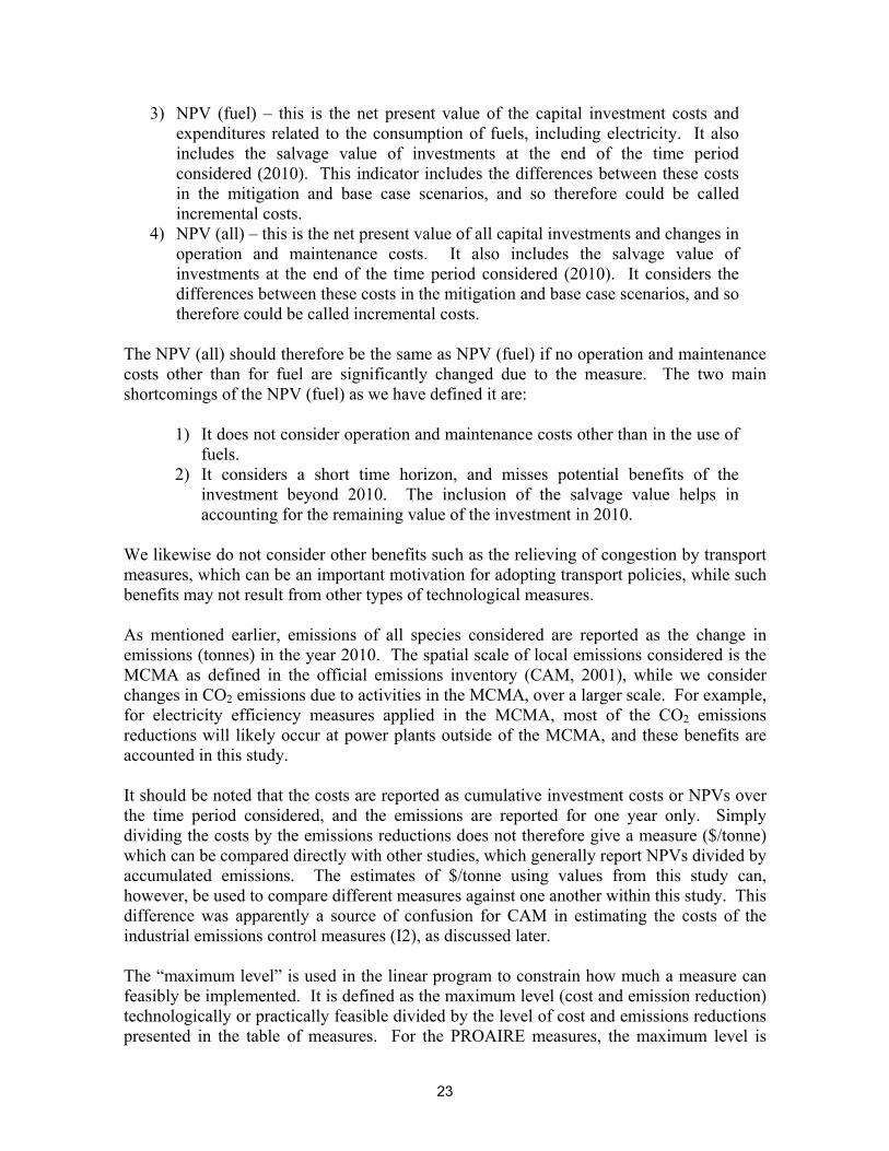
We likewise do not consider other benefits such as the relieving of congestion by transport measures, which can be an important motivation for adopting transport policies, while such benefits may not result from other types of technological measures. As mentioned earlier, emissions of all species considered are reported as the change in emissions (tonnes) in the year 2010. The spatial scale of local emissions considered is the MCMA as defined in the official emissions inventory (CAM, 2001), while we consider changes in CO2 emissions due to activities in the MCMA, over a larger scale. For example, for electricity efficiency measures applied in the MCMA, most of the CO2 emissions reductions will likely occur at power plants outside of the MCMA, and these benefits are accounted in this study. It should be noted that the costs are reported as cumulative investment costs or NPVs over the time period considered, and the emissions are reported for one year only. Simply dividing the costs by the emissions reductions does not therefore give a measure ($/tonne) which can be compared directly with other studies, which generally report NPVs divided by accumulated emissions. The estimates of $/tonne using values from this study can, however, be used to compare different measures against one another within this study. This difference was apparently a source of confusion for CAM in estimating the costs of the industrial emissions control measures (I2), as discussed later. The “maximum level” is used in the linear program to constrain how much a measure can feasibly be implemented. It is defined as the maximum level (cost and emission reduction) technologically or practically feasible divided by the level of cost and emissions reductions presented in the table of measures. For the PROAIRE measures, the maximum level is

24

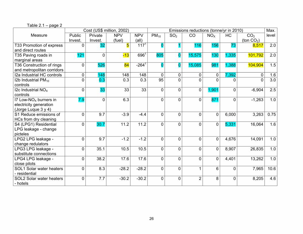
defined relative to the level implemented in PROAIRE (the level of activity in PROAIRE is defined as 1.0 for all measures). In most cases, the maximum level was defined on the basis of information in the documents available or the calculations spreadsheets, which indicates the potential applicability of the measure. For measure V21, the accelerated retirement of old vehicles, for example, we find the measure to be ambitious in replacing nearly 1 million private vehicles over the 9 years considered. We do not therefore assume that a greater rate of retirement is plausible. However, the measure is only applied in the Federal District, and could potentially be applied also to the State of Mexico. For this reason, we chose 1.5 as the maximum level, reflecting the relative fleet sizes in the DF and State of Mexico. 2.4 Coherent Database of Options The database of options is presented in Table 2.1. Estimates that are still preliminary due to a lack of information are marked in yellow. These estimates use the best information currently available, but should be pursued further in the future by searching for better information. For the PROAIRE measures, numbers marked in blue represent a significant change from the estimate reported in PROAIRE.

25

Table 2.1 – Summary of the measures for controlling emissions, applicable in the Mexico City Metropolitan Area. Estimates in blue represent changes from PROAIRE, and numbers in yellow signify estimates which could be improved with acquisition of better data.

Cost (US$ million, 2002) Emissions reductions (tonne/yr in 2010) Measure Public

Invest. Private Invest.

NPV (fuel)

NPV (all)

PM10 SO2 CO NOX HC CO2 (ton CO2)

Max. level

V1&2 Tier II for new private vehicles, low S gasoline

470 340 305 469 426 159 10,482 11,006 3,564 -87,185 1.0

V6 Retrofit private vehicles with catalyst

0 163 182 0 0 142,937 1,637 11,703 -23,885 1.0

V8 Substitute old taxis & Tier II taxis

80 720 690 124 0 85,108 8,579 11,434 21,122 1.1

V9 Substitute old microbuses for new buses of greater capacity

21 971 -130 -1079 12 0 149,176 5,027 13,374 454,362 1.0

V12&13 Advanced emissions controls for new diesel vehicles, low S diesel

147 166 161 640 40 0 6,362 1,012 -45,515 1.0

V21 Eliminate old private vehicles

827 8,600 3,615 0 0 583,211 15,239 55,298 495,685 1.5

V22 Substitute RTP and STE buses

124 0 101 95 0 725 860 348 17,465 1.0

V23 Eliminate old gasoline light trucks

274 1,272 528 24 0 86,829 6,131 5,728 342,189 1.8

T25 Expansion of the Metro

3,938 0 1,211 4681 352 91 9,375 7,074 2,841 144,386 1.2

T26 Establish a network of suburban trains

1,020 0 246 10231 265 72 7,064 5,330 2,140 0 1.5

T27a Grow network of trolleybuses

1,556 0 193 3381 701 192 20,250 14,668 5,965 517,840 1.5

T27b Grow network of light rail

1,348 0 312 4151 228 60 6,186 4,631 1,864 147,527 1.2

T28 Bases for taxis 0 13 -29 1701 0 12 6,048 115 469 36,582 1.5

26

Table 2.1 – page 2 Cost (US$ million, 2002) Emissions reductions (tonne/yr in 2010)

Measure Public Invest.

Private Invest.

NPV (fuel)

NPV (all)

PM10 SO2 CO NOX HC CO2 (ton CO2)

Max. level

T33 Promotion of express and direct routes

0 32 5 1171 0 1 116 156 73 8,517 2.0

T35 Paving roads in marginal areas

121 0 -13 6961 805 0 15,575 130 1,335 101,792 2.0

T36 Construction of rings and metropolitan corridors

0 526 84 -2641 0 0 15,085 981 1,388 104,904 1.5

I2a Industrial HC controls 0 148 148 148 0 0 0 0 7,392 0 1.6 I2b Industrial PM10 controls

0 0.3 0.3 0.3 95 0 0 0 0 0 3.0

I2c Industrial NOX controls

0 33 33 33 0 0 0 1,901 0 -6,904 2.5

I7 Low-NOX burners in electricity generation (Jorge Luque 3 y 4)

7.9 0 6.3 0 0 0 871 0 -1,263 1.0

S1 Reduce emissions of HCs from dry cleaning

0 9.7 -3.9 -4.4 0 0 0 0 6,000 3,263 0.75

S4 (LPG1) Residential LPG leakage - change picteles

0 30.7 11.2 11.2 0 0 0 0 5,331 16,064 1.6

LPG2 LPG leakage - change redulators

0 9.7 -1.2 -1.2 0 0 0 0 4,676 14,091 1.0

LPG3 LPG leakage - substitute connections

0 35.1 10.5 10.5 0 0 0 0 8,907 26,835 1.0

LPG4 LPG leakage - close pilots

0 38.2 17.6 17.6 0 0 0 0 4,401 13,262 1.0

SOL1 Solar water heaters - residential

0 8.3 -28.2 -28.2 0 0 1 6 0 7,965 10.6

SOL2 Solar water heaters - hotels

0 7.7 -30.2 -30.2 0 0 2 8 0 8,205 4.6

27

Table 2.1 – page 3 Cost (US$ million, 2002) Emissions reductions (tonne/yr in 2010)

Measure Public Invest.

Private Invest.

NPV (fuel)

NPV (all)

PM10 SO2 CO NOX HC CO2 (ton CO2)

Max. level

SOL3 Solar water heaters - hospitals

0 12.3 -44.9 -44.9 0 0 3 11 0 13,029 3.6

SOL4 Solar water heaters - public baths

0 0.6 -2.0 -2.0 0 0 0 1 0 785 1.03

HYB1 Hybrid buses for RTP (SKI)

304 0 259 84 0 712 922 334 98,433 1.0

HYB2 Hybrid buses for RTP (MP)

201 0 130 96 0 760 1,064 362 86,426 1.0

HYB3 Hybrid buses for RTP (TRANSTEQ)

489 0 412 83 0 703 906 331 96,058 1.0

HYB4 Hybrid buses for RTP (ORION)

489 0 391 50 0 399 364 219 9,631 1.0

G2 Efficient lighting - residential

0 44 -165 -165 1 0 5 45 0 460,000 1.0

G3 Efficient lighting - commercial

0 252 -100 -100 1 0 4 36 0 369,000 1.0

G4 Efficient pumping of potable water

147 0 -79 -79 0 0 3 21 0 279,000 1.0

G5 Efficient electric motors in industry

0 65 171 171 0 0 2 20 0 207,000 1.0

G7 Industrial cogeneration of heat and electricity

0 1,083 -1,158 -1,158 6 1 51 434 2 4,424,000 1.0

G11 Forest restoration 1.6 0 0.9 0.9 0 0 0 0 0 22,000 1.0 G12 Agroforestry options 0.1 0 0.1 0.1 0 0 0 0 0 4,000 1.0

NOTES 1 These NPV (all) values come from the report of COMETRAVI (1999), and include the costs of travel time, operation and maintenance, and use a discount rate of 12%.

28

Table 2.2 – Measures that apply in Mexico, outside of the MCMA, and which have no effects on local emissions within the MCMA. Cost (US$ million, 2002) Emissions reductions (tonne/yr in 2010)

Measure Public Invest.

Private Invest.

NPV (fuel)

NPV (all)

PM10 SO2 CO NOX HC CO2 (ton CO2)

Max. level

GN2 Efficient lighting – residential

0 196 -729 -729 0 0 0 0 0 2,040,000 1.0

GN3 Efficient lighting – commercial

0 569 -227 -227 0 0 0 0 0 831,000 1.0

GN4 Efficient pumping of potable water

491 0 -261 -261 0 0 0 0 0 921,000 1.0

GN5 Efficient electric motors in industry

0 219 575 575 0 0 0 0 0 693,000 1.0

GN7 Industrial cogeneration of heat and electricity

0 7,581 -8,108 -8,108 0 0 0 0 0 30,976,000 1.0

GN8 Wind electricity generation

5,000 0 -1,131 -1,131 0 0 0 0 0 12,200,000 1.0

GN9 Temperate forest management

639 0 -3,852 -3,852 0 0 0 0 0 141,100,000 1.0

GN10 Tropical forest management

51 0 775 775 0 0 0 0 0 62,000,000 1.0

GN11 Forest restoration 873 0 505 505 0 0 0 0 0 12,000,000 1.0 GN12 Agroforestry options

68 0 68 68 0 0 0 0 0 2,000,000 1.0

29

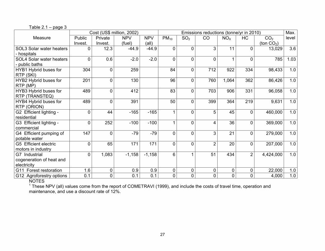
In the case of the GHG mitigation measures, two measures (expanding the Metro and using larger buses) were eliminated since they were the same as PROAIRE measures, and more information exists for the PROAIRE measures. Other measures were not included due to a lack of information in the studies that would be needed to estimate investment costs and emissions reductions. In Table 2.1, GHG mitigation measures are listed only as they apply to the MCMA. Table 2.2 lists GHG mitigation measures that apply outside of the MCMA, on a national scale (denoted as GN), which have no concurrent benefits for local air pollutants in the MCMA. Our plan is to conduct the analysis under two different assumptions: one which restricts all emissions reductions activities to the metropolitan area (using only Table 2.1), and one which allows GHG mitigation to be purchased outside of the MCMA (allowing both urban and national measures as separate options). 2.4.1 PROAIRE measures In this section, we describe the principal assumptions and corrections for each measure individually. Complete notes on the measures in PROAIRE are given (in Spanish) in Appendix A. Excel spreadsheets submitted with this final report show the cost and CO2 emissions reduction calculations for the PROAIRE measures. V1&2 Tier II for new private vehicles, low S gasoline – Costs for this measure are less than in PROAIRE because PROAIRE reports the cost of producing low S gasoline on a national scale, with the national scale estimate produced by PEMEX. Here we corrected this cost according to the consumption of fuel in the MCMA. A US EPA (1999) study on the implementation of Tier II with low-S gasoline indicates that the Tier II technology has no effect on fuel consumption, but that the refining of low-S gasoline is associated with an increase in CO2 emissions. Here we scale the CO2 emissions with the estimated increase in the US, using the relative amounts of gasoline consumption in the MCMA versus the entire US. V6 Retrofit private vehicles with catalyst – Emissions are less than in PROAIRE because PROAIRE calculates the effect of this measure together with Tier II, which would be double-counting the Tier II effect. For CO2 emissions, the catalyst is thought to decrease efficiency by causing back pressure on the engine. We have yet to find a good estimate of the effect of the retrofit on efficiency, and are currently assuming a loss of efficiency of 2%. V8 Substitute old taxis & Tier II taxis – Although it does not mention this in PROAIRE, this measure is actually a combination of a substitution program and Tier II taxis starting in 2006. We use IPCC emissions factors for vehicles to calculate the CO2 emissions – the calculation could be improved if we can get data on fuel efficiency for in-use Mexico City vehicles, but our investigations suggest that these data may not exist. V9 Substitute old microbuses – This measure replaces old gasoline microbuses with new larger buses which are either gasoline or diesel. The cost in PROAIRE is apparently based on US$46,000 per new bus, the reason for which we do not know. We changed the cost using US$60,000 for diesel and gasoline buses, and US$80,000 for CNG buses. The reduced CO2 reflects the assumption in PROAIRE that these larger buses (with greater

30

capacity) require fewer vehicle-km traveled for the same service. The negative NPV (all) reflects mainly the reduced number of drivers needed. V12&13 Emissions limits for diesel, low S diesel – The costs of refining low S diesel are from PEMEX (national) and are corrected for the MCMA, as was done for V1&2. For the CO2 emissions, we assume that the increase in CO2 from producing low sulfur diesel is the same per liter as for gasoline in V1&2. We use IPCC emissions factors for CO2, and assume a 2% loss of efficiency due to the emissions controls on heavy diesel, based on a study of heavy diesel emissions controls by the US EPA (2002). V21 Eliminate old private vehicles – We estimate costs here using US$11,400 for a new vehicle, which is considerably greater than the unit cost used in PROAIRE (US$4,700). We do not have an explanation for the costs of this measure in PROAIRE, but since the emissions reductions are calculated using new vehicles, the cost should reflect a new vehicle. We also feel that the emissions reductions estimates in PROAIRE for this measure are far too low, because of their methods of projecting the fleet under the control scenario. Our recalculation increases the emissions reductions substantially. We use IPCC emissions factors for vehicles of different ages to calculate the CO2 emissions. As for the other transport measures, our estimate of changes in CO2 emissions could be improved with data on the efficiency of in-use vehicles in Mexico City. V22 Substitute RTP and STE buses – This measure substitutes publicly owned diesel buses with CNG buses. The increase in cost relative to PROAIRE is due to an apparent error in PROAIRE between US$ and Mexican pesos. CO2 emissions are based on tailpipe emissions only, for a net CO2 savings. Field tests of CNG buses (NAVC et al., 2000) suggest that because of CH4 leakage, net GHG emissions may be higher from CNG buses, but we do not consider this here. This is the only measure where CH4 or N2O is likely to be important for GHG emissions. V23 Eliminate old gasoline light trucks – CO2 emissions are based on IPCC emissions factors. Note that no gasoline light trucks are reported for the State of Mexico in the emissions inventory. We therefore assumed that the measure could be applied to the State of Mexico in the maximum level chosen for this measure. T25 Expansion of the Metro – All of the transport measures (T) are based on estimates from COMETRAVI (1999) and used directly in PROAIRE. Emissions in COMETRAVI (1999) are estimated assuming that the Metro replaces (avoids) diesel buses – we used emissions factors to infer the number of diesel bus km avoided by the Metro. We considered also the CO2 emissions from diesel buses and the electricity used by the Metro. T26 Network of suburban trains – The cost in PROAIRE for this measure is US$15 million total. It should be US$15 million per km of train, and so we used this unit cost to derive a total cost which is higher than the cost in COMETRAVI (1999). We have calculated the diesel bus km avoided because of the suburban trains, but we do not know the use of fuel by these suburban trains. Based on the information we have found, the fuel consumption and CO2 emissions of trains may be greater or less than diesel buses, and so we assume no change.

31

T27a Grow network of trolleybuses – In PROAIRE, there was some confusion in taking the costs and emissions reductions from the COMETRAVI (1999) study, and our correction of these errors decreases the emissions reductions substantially. The NPV (fuel) and CO2 emissions are calculated as for the Metro (T25), but using inferred figures for the electricity consumption by trolleybuses – the uncertainty in this measure could be reduced by finding a more reliable figure. T27b Grow network of light rail – The NPV (fuel) and CO2 emissions are calculated as for the Metro (T25), but using inferred figures for the electricity consumption by trolleybuses – the uncertainty in this measure could be reduced by finding a more reliable figure. T28 Taxi bases – The measure is estimated to cause a reduction in taxi-km which we estimate to be about 2%, by reducing the roaming of taxis looking for customers. The negative NPV (fuel) reflects the savings of fuel. T33 Express and direct routes – Costs and emissions reductions of local pollutants were taken from COMETRAVI (1999). The effect of this measure is to both reduce the travel distance and increase the average velocity for diesel buses. We model the change in diesel consumption as if the local emissions avoided were due entirely to a reduction in bus-km. T35 Paving roads in marginal areas – Costs and emissions reductions of local pollutants were taken from COMETRAVI (1999). This measure directly reduces PM emissions, and causes vehicle emissions to decrease by increasing velocity (based on information in COMETRAVI (1999), the increases in velocity would be expected to be in the range where increases in velocity decrease emissions). We lack information on how emissions change as a function of velocity, and so we estimate the change in fuel consumption as if the local emissions avoided were due entirely to a reduction in vehicle-km traveled. T36 Construct rings and metropolitan corridors – Costs and emissions reductions of local pollutants were taken from COMETRAVI (1999). The same note applies as for the previous measure, except that there is no direct reduction in PM emissions. I2 Industrial emissions controls (on HCs, NOX, and PM10) – We divided this measure into three measures since PROAIRE presents costs and emissions reductions for each pollutant independently. Our costs are significantly higher than in PROAIRE because of what we see as error in how the $/ton values from the literature were used – the $/ton from the literature were multiplied by the 2010 emissions reductions in PROAIRE rather than the accumulated emissions over the project lifetime, which we understand to be about 10 years. We assume also that the costs are up front and there are little extra operation and maintenance expenditures, so that the investment costs are equivalent to the NPV values from the literature ($/ton). For low-NOX burners, we use information from the IPCC (1996) that suggests a loss of efficiency of 0.25%, to estimate CO2 emissions. I7 Low-NOX burners in local power plants – PROAIRE shows an emissions reduction of 4,000 tons/yr and no cost, for a number of individual measures to be applied to the two local power plants. Of these measures only two are well-defined: installing low-NOX

32

burners in units 3 and 4 of Jorge Luque and repowering unit 4 of Valle de Mexico. We use costs and emissions reductions for low-NOX burners for units 1 and 2 of Jorge Luque from Morales (2001), and correct for the size of units. For the repowering option, we lack sufficient data since the repowering would increase capacity and its effect on emissions is not clear from Morales (2001). We use a loss of efficiency of 0.25% from the IPCC (1996) to estimate CO2 emissions. S1 Reduce dry cleaning emissions – The measure reduces emissions of perchloroethylene to the atmosphere. The negative NPV (fuel) reflects the value of perchloroethylene which is saved. Perchloroethylene does not have global warming potential. We account for its effect on CO2 emissions by accounting for its carbon content, since perchloroethylene would be converted to CO2 in the atmosphere (the lifetime of perchloroethylene in the atmosphere is about five months). S4 (LPG1) Change picteles – The PROAIRE measure to reduce residential leakages of LPG in homes is based on changing picteles in stoves. Here we use the TUV study to re-estimate these costs and emissions reductions. Emissions of CO2 are estimated using the carbon content of the LPG, since the LPG would be converted to CO2 in the atmosphere (the lifetimes of propane and butane in the atmosphere are on the order of weeks). 2.4.2 GHG mitigation measures As mentioned earlier, the final costs in the GHG mitigation studies are reported as US$ per tonne of CO2, where the cost is the annualized cost of the measure. From these reports, it is not clear whether these costs are divided by the cumulative change in emissions over the project time horizon (1997-2010), or by the change in emissions in one year. Upon reviewing this issue, we have concluded that the emissions reductions (to which the costs refer) must be annual emissions in 2010 (tonnes CO2 per year). We have three reasons for believing this:

1) The accumulated emissions are never reported in any of the documents, only the annual emissions in 2000, 2005 and 2010.

2) When we used the assumption that costs refer to accumulated emissions, the NPV values were implausibly large in comparison with our estimated investment costs.

3) When we tried to recreate the cost estimates using information from the documents (for residential lighting and a few other measures which provided relatively more information), we could not reproduce the $/ton figures assuming that costs refer to accumulated emissions, and achieved better agreement when assuming that costs refer to 2010 emissions.

For each of the GHG measures, it is necessary to estimate the extent to which the measure applies in the urban area, estimate changes in emissions of local air pollutants for those measures which apply to the metropolitan area, estimate the direct investment costs based on information in the available documentation, and convert the reported costs from annualized costs to NPVs.

33

For the measures that reduce electricity consumption (measures G2, G3, G4, G5, and G7), many plausible assumptions can be made for the change in electricity generation and power plant emissions resulting from the reduced electricity consumption in the metropolitan area. Mexico City differs from many urban areas in that the majority of the electricity consumed (about 80%) is imported from other states. Only two large base load plants and three small peaking plants exist in the area considered for the emissions inventory (the geographical limits of this study), although other power plants, including the plant at Tula, likely has some effect on Mexico City air quality (which is not well understood). We have made calculations of the change in emissions from the local power plants, caused by reduced electricity consumption in the metropolitan area, under four scenarios:

1) The reduced electricity consumption reduces generation from plants entirely outside of the metropolitan region. Under this scenario, there is no change in emissions from the local power plants. (0% of reduced local consumption comes from local plants)

2) The reduced electricity consumption reduces generation entirely from the plants within the metropolitan region. (100%)

3) The reduced electricity consumption is distributed equally over all plants in the interconnected electrical grid (most of Mexico). (3.1%)

4) The reduced electricity consumption is distributed according to the ratio of consumption in the MCMA with the generation in the MCMA. (20.7%)

The results for one measure, residential efficient lighting, are shown in Table 2.3. The four scenarios shown are meant to reflect the range of possible results, but which is most plausible? Plans for electricity in the metropolitan area suggest that there will be little change in the generation of the two large base plants, as these are necessary to maintain grid stability as electricity demand continues to grow in the future. Changes in emissions from the peaking plants due to these measures may be more likely, and we should also consider that emissions from other plants, outside of the metropolitan area have some effect on air quality. For these reasons, we consider Scenarios 1, 3, and 4 to be plausible, and selected Scenario 3 as our best guess to present in Tables 2.1 and 2.2. Future work using the quantitative decision-making techniques (linear programming) can analyze the sensitivity of the results to which scenario we choose.

Table 2.3 – Reductions in emissions of local air pollutants from residential efficient lighting under four electricity scenarios (tons per year in 2010).

Scenario PM10 SO2 CO NOX HC 1 0 0 0 0 0 2 21.04 2.44 169.35 1454.17 7.32 3 0.65 0.08 5.27 45.21 0.23 4 4.36 0.51 35.11 301.49 1.52

Using scenario 3 for all of the measures that reduce electricity consumption, we find that the reduction in local air pollutants is small in all cases except for G7, industrial cogeneration. For industrial cogeneration, the report indicates a very large potential for

34

CO2 reduction by industrial cogeneration nationally, suggesting that the potential local application may be large (Tables 2.1 and 2.2). Since there is the suggestion that the application of cogeneration may be large, its applicability on the scale of the MCMA should be reviewed further. For costs, we find that for most measures, changes in operation and maintenance costs are likely to be zero or very low for the efficient technologies – for several measures, the GHG mitigation studies state that these costs are zero. We can therefore take the NPV (all) from the study and assume that it is a good measure of NPV (fuel) to be compared directly with the PROAIRE measures. Notes on individual measures in Tables 2.1 and 2.2 follow: G2 Residential efficient lighting – Emissions reduction potential is distributed locally and nationally using the number of households. Investment costs are simply the costs of compact fluorescent lightbulbs, as reported in Sheinbaum (1997), including replacements through the time horizon considered, but not considering avoided costs of conventional bulbs (which is included in the NPV). For this measure, there are no operation and maintenance costs beyond the cost of electricity, so the NPV (all) can be assumed to be the same as the NPV (fuel). G3 Commercial efficient lighting – Distributed locally and nationally using the economic production from the commercial sector. Investment costs are calculated like the residential (G2), but with higher unit costs. There are no operation and maintenance costs beyond the cost of electricity, so the NPV (all) can be assumed to be the same as the NPV (fuel). G4 Potable water pumping – Distributed locally and nationally using the number of households with access to potable water. The investment cost is based on pilot projects reported in Sheinbaum (1997). The measure proposes to replace or perform maintenance on water pumps, beyond which no further maintenance is expected in the time horizon considered, so that NPV (fuel) = NPV (all). G5 Electric motors in industry – Distributed locally and nationally using the economic production of manufacturers. The unit investment cost is US$411.50 for a high efficiency motor (averaged over a range of sizes). According to Sheinbaum (1997), the maintenance costs of high efficiency motors are the same as conventional motors, so NPV (fuel) = NPV (all). G7 Industrial cogeneration – The maximum level in Sheinbaum and Masera (2000) assumes that all new industrial plants will use cogeneration systems. The measure is distributed locally and nationally assuming that new petrochemical and fertilizer plants would be entirely outside of the metropolitan region, while new chemical and pulp and paper plants would follow the existing national distribution (using economic production data). According to Sheinbaum (1997), the unit investment cost is US$1000 per 1 kW installed capacity, and operation and maintenance costs are negligible in comparison to investment costs, so NPV (fuel) = NPV (all).

35

GN8 Wind electricity generation – This measure does not apply on the metropolitan scale. An investment cost of US$1000 per installed kW capacity was used (from Sheinbaum (1997)). The negative NPV in Sheinbaum and Masera (2000) must indicate that the wind generation produces electricity more cheaply than conventional systems, but we do not know what electricity cost they are comparing against. Operation and maintenance costs are not negligible, and so this is one measure where the NPV (fuel) may not equal the NPV (all), which should be investigated further. GN9 Temperate forest management – This measure does not apply on the metropolitan scale. Investment costs are taken from the report, using costs from pilot projects. According to Sheinbaum (1997), the NPV is negative because of the opportunity cost of the land – evidently, the land is considered to be worth more in forest management than the alternative considered. GN10 Tropical forest management – This measure does not apply on the metropolitan scale. Investment costs are taken from Sheinbaum (1997), using costs from pilot projects which represent the cost of the land. G11 Forest restoration – This measure is assumed applicable to the metropolitan area accoring to the fraction of the nation’s total area (0.18%) – note that the metropolitan area defined by the emissions inventory includes large areas that could be applicable for forest restoration or agroforestry. Investment costs are taken from Sheinbaum (1997), using costs from pilot projects which represent the cost of the land. G12 Agroforestry options – This measure is assumed applicable to the metropolitan area accoring to the fraction of the nation’s total area (0.18%). Investment costs are taken from the report, using costs from pilot projects which represent the cost of the land. For all of the forestry measures (G9-G12), it is appropriate to include the opportunity cost as part of NPV (fuel) since this represents the baseline assumption. Consequently, the NPV (fuel) can be assumed to be the same as the NPV (all) given in the studies, although future research should investigate further the operation and maintenance costs. 2.4.3 Other studies of emissions reduction technologies The study by TUV Rheinland (2000) of measures to reduce domestic leakages of LPG includes several individual measures that could be applied. Of these measures, we chose to model four which had the lowest costs according to the study, and which can be applied independently of one another. We modeled these measures following the schedule of implementation for the LPG leakage measure in PROAIRE (S4), of implementing the measure for 1 million homes by 2010. The costs include also the cost of replacing the technology before 2010, as the lifetimes of these technologies are short. The study by Quintanilla et al. (2000) gives the estimated costs and emissions reductions of pilot programs to install solar hot water heaters in homes, hotels, hospitals, and public baths. The information in the document is sufficient to esitmate the investment costs and NPVs – we used the costs without financing and assumed that the old LPG, gas, or diesel

36

systems were kept as backups to the solar system. The emissions reductions reflect the reduced emissions during combustion – there may be additional reductions due to reduced leakages of LPG, but because the LPG system is kept as a backup, the hydrocarbon emissions reductions are expected to be low. The maximum level for this technology is estimated based on information in the document. The document on hybrid electric buses (Consultants to the World Bank, 2000) provides basic cost and emissions data for four models of hybrid electric buses, as well as new gasoline, diesel, and CNG buses, for direct comparison. The report is written for public buses for the RTP system, and so we consider these technologies as alternatives to replacing all of the the diesel RTP buses with CNG buses in measure V22. Emissions reductions and costs are therefore modeled in exactly the same manner as measure V22, but with different unit costs and emissions factors for each bus type. Since V22 replaces all of the RTP buses with CNG buses, it is not possible to also replace them with hybrid buses. An extra constraint will therefore be required to force the LP to keep from duplicating the replacement of RTP buses. This is the only measure for which such an extra constraint will be necessary. 2.5 Overall Assessment of Database of Options Overall we feel that the database of options is self-consistent in that the same methodology was applied to different measures, and therefore, that the numbers for the different measures can be compared directly against one another. In constructing this database, we made use of the available information from studies in Mexico, and further, went beyond these studies in terms of estimating emissions reductions of other pollutants and costs that were not reported in these studies. In addition, we reviewed carefully and made changes to the values reported in PROAIRE, where we thought that there were errors or differences of opinion at a very basic level. In reviewing PROAIRE and other studies, we observed many cases where there were methodological problems in the costs or estimations of emissions reductions – the manner used to project the future vehicle fleet composition, for example, causes uncertainties which underlie the emissions reductions estimated for several measures. Correcting or changing the estimates from previous studies at this more detailed or methodological level was beyond the scope of this study. We therefore feel that we strike a good balance in improving the information available and creating a consistent database, without going to the level of revising the methodologies used, which is beyond the scope of this study. Working at this level would be necessary to achieve further improvements in the database, and we suggest that long-term improvements in quantitative estimates of the costs and emissions reductions associated with different controls measures need to begin by improving calculations at a fundamental level. While we are confident in our database, however, there are several methodological issues which create uncertainty in our results and limit the confidence with which we can draw conclusions using this database:

1) The results of this study are based almost entirely on previous studies conducted in Mexico. Each of these studies has its own uncertainties and

37

methodological assumptions, and as we have reviewed these studies, we have become more aware of their limitations. The lack of documentation has been a serious problem in understanding the studies and their shortcomings, and highlights the need to better document economic and emissions calculations.

2) We use the NPV (fuel) in place of a full calculation of the NPV (all) as a basis for comparing the measures. While this is a limitation, it is the best feasible in the time frame for this project, and with the number of measures that we are dealing with. The complexity of estimating the NPV (all) in a coherent way for a single measure can be seen in the World Bank study of Mexico City (Cesar et al., 2002) and recent reviews conducted in the US by the EPA (US EPA, 1999; US EPA, 2002).

3) Emissions reductions are presented as a snapshot in 2010, while costs are aggregated over the time period (investment costs as a simple sum and NPVs as a discounted sum). Consequently, the emissions and costs for a given measure cannot be compared directly, nor can they be compared directly against $/ton values in the literature (which are generally NPVs divided by accumulated emissions). This method of presenting results was selected to be consistent with PROAIRE, but we suggest that future work consider estimating the entire time profile of emissions, and consider using some summary measures of this time profile, such as the aggregated or discounted changes in emissions.

4) We consider a limited time horizon of up to 2010, which is consistent with the studies that we consider. This has the disadvantage that we do not consider benefits beyond 2010 in our NPV calculations. We do, however, account for the salvage value of investments in 2010, to address the differences between measures where the investment is up front and the lifetime of the technology is short (e.g., catalyst retrofits), and other measures where investments occur annually until 2010 and where the lifetime is long (e.g., the Metro expansion). In future work, we suggest considering a longer time horizon – we chose not to do this now because we lack basic information beyond 2010 (e.g., we do not have a projection of the vehicle fleet after 2010).

5) The emissions reductions of different measures are assumed to be independent and additive in a simple way. Some combinations of measures may not, however, be additive simply. For example, applying Tier II technology and accelerating the retirement of old vehicles likely results in emissions reductions larger than the sum of doing the two individually. Investing in new buses and expanding the Metro will result in a net emissions reduction less than the sum of the two individual measures. While it is possible to address this complexity in a linear program, this assumption is consistent with PROAIRE, which simply adds emissions reductions from each measures, and this complexity is beyond the scope of this study.

6) We consider tons of each pollutant to be interchangeable, regardless of the location and time of emissions. Likewise, we assume all emissions of hydrocarbons (and PM10) to be equivalent, although the net effects of different species on health may be very different. Again, this is consistent with PROAIRE which simply adds the total emissions of each pollutant. Future work could consider using air quality models to assess the changes in ozone or PM10 resulting from changes in emissions from different source categories.

38

7) We currently consider only CO2 emissions, and not emissions of other GHGs. This is probably a good assumption for nearly all measures, with some exceptions such as CH4 from CNG buses. The effect of fugitive emissions of percholoroethylene and of LPG on climate should also be reconsidered in the future.

8) In using the linear programming, we assume that the costs and emissions reductions are linear as the “activity level” of the measure changes. That is, we assume that the marginal cost is equal to the average cost – we can do more or less of a measure (within its maximum activity level) with the costs and emissions reductions being proportional.

9) Finally, in using the LP, we assume that this list of measures is comprehensive in including all emissions reductions options. Certainly other emissions reductions possibilities exist for the MCMA, which are not included in this study because they have not been previously studied for Mexico City.

2.6 Net results of database of options Table 2.4 shows the net results of 22 PROAIRE measures listed in Table 2.1, in comparison with the figures that appear in the PROAIRE document. First, we find very good agreement when comparing the costs and emissions reductions from PROAIRE for the measures included in this study, with the PROAIRE totals. This suggests that we are indeed capturing the quantitatively most important measures in this study, with the exception of SO2 – most of the SO2 reductions in PROAIRE come from one industrial measure that we do not include. The differences between our estimates and those in PROAIRE (Table 2.4) are seen to be substantial, with higher costs overall, and substantially higher emissions reductions for CO, and significant changes for other pollutants. The higher public investment cost in this study can be attributed mainly to the fact that we show a cost from COMETRAVI (1999) for some measures for which a cost was not listed in PROAIRE, notably for the Metro expansion. The higher private investment cost is due mainly to the increased cost of measure V21, through our use of the cost of new vehicle, which is higher than the unit cost in PROAIRE. The increase in CO and HC emissions reductions in this study can likewise be attributed to measure V21, because of our changes in modeling the vehicle fleet when the measure is applied. The decrease in NOX emissions relative to PROAIRE can be attributed mainly to the error in taking emissions from COMETRAVI (1999) for T27a (trolleybuses), and secondarily to the inclusion in PROAIRE of Tier II emissions reductions reported together with measure V6 (catalyst retrofits). The emissions reductions estimated in this study can likewise be compared against recent emissions inventories and projections of emissions to 2010 (Table 2.5), to ensure that the emissions reductions are reasonable. The percent reduction in emissions in 2010 due to PROAIRE and the other emissions reductions measures are shown in Table 2.6. The results show that the PROAIRE is an ambitious plan to reduce a large fraction of several pollutant emissions, but that the results do not exceed the total emissions. When the

39

maximum level is used for all PROAIRE measures, the total emissions reductions do not exceed the 2010 emissions for any pollutant. Even when we apply all measures at their maximum level of implementation on the MCMA scale (all measures in Table 2.1), we do not exceed any of the emissions in the 2010 inventory, although the total emissions reductions would be substantial from fully implementing all of these measures. We likewise checked that the emissions reductions from each individual measure do not exceed the total 2010 emissions from that category of emissions. An important outcome of this research is our estimate of the CO2 emissions consequences of implementing all of the PROAIRE actions at the level proposed in PROAIRE. Our estimate shows a significant reduction of CO2 emissions due to the PROAIRE actions, of 2.2 million tonnes of CO2 in 2010. Comparing this with our projection of CO2 emissions in 2010, this reduction is about 3.1%. While this is smaller than the reduction seen for the emissions of criteria pollutants, it still represents a significant reduction. This reduction could be thought of as an “ancillary benefit”, “secondary benefit”, or “co-benefit” of urban air pollution control in the MCMA. Interestingly, the reduction in CO2 emissions results about equally from vehicle technology measures (1.2 million tonnes in 2010) as from transportation measures (1.1 million tonnes). Industrial and services measures have very little effect on CO2 emissions. It is also interesting to note that five measures listed cause a net increase in CO2 emissions, due to a loss of energy efficiency – the greatest of these CO2 increases is due to the refining of low-S gasoline (V1&2). For the measures not included in PROAIRE (the “GHG measures”), when applied to their maximum extent on the metropolitan scale, the reduction in emissions of CO2 is 8.7% of the 2010 emissions. Meanwhile, the potential for these measures to reduce emissions of local pollutants is rather small, but not insignificant: 1.3% percent of PM10, 1.4% of NOX, and 3.2% of HCs – the fact that the percentage decrease is largest for HCs is due mainly to the LPG leakage measures. Again, the conclusion that these measures have a small effect on emissions of local air pollutants depends in part on our assumptions of how emissions from local electricity generation changes due to the measures which reduce electricity consumption. Further, it is important to note (in Table. 2.4) that while these measures increase the investment costs significantly, they cause a net decrease in the NPV (fuel), reflecting that many of these measures are estimated to come at a net cost savings.

40

Table 2.4 – Summary of results for the air quality and GHG control measures applied on the scale of the MCMA (from Table 2.1). The results from this study for the PROAIRE measures are compared with the totals reported in PROAIRE.

Cost (US$ million, 2002) Emissions reductions (tonne/yr in 2010) Measure Public

Invest. Private Invest.

Total Invest.

NPV (fuel)

PM10 SO2 CO NOX HC CO2 (ton CO2)

PROAIRE Total 6,529 7,740 14,269 4,913 5,180 591,206 121,096 99,907 PROAIRE – 22 Measures included in Table 2.1. 6,330 7,740

14,070

4,887 972 590,972 115,622 99,880

This study – Total of 22 Measures from PROAIRE 9,934 13,025 22,959 7,656 3,767 627 1,138,167 90,698 137,259 2,246,946 This study – 22 PROAIRE Measures applied at maximum level 13,041 18,871 31,912 10,645 5,393 796 1,550,773 120,106 184,098 3,267,473 This study – All other measures (18 not in PROAIRE) applied locally at maximum level 1,631 1,695 3,326 -714 321 1 2,670 3,953 19,232 6,279,621 This study – All Measures applied At maximum level 14,671 20,566 35,237 9,931 5,714 797 1,553,443 124,059 203,330 9,547,094

41

Table 2.5 – Total MCMA emissions. PM10 SO2 CO NOX HC CO2

(ton CO2) Total emissions 1998 1 19,889 22,466 1,768,836 205,885 475,021 1998 IPCC 1 37,504,977 1998 US EPA 1 16,699,861 1996 MCMA 2 34,850,000 1996 including electricity outside 2

45,585,000

Total emissions 2010 3 25,141 32,721 2,270,301 281,781 594,323 2010 MCMA projected 4

71,800,000

1 CAM (2001), estimated using IPCC and US EPA emissions factors. 2 Sheinbaum et al. (2000), estimated for the metropolitan area only, and including CO2 from the local consumption of electricity generated outside of the metropolitan area. 3 Cesar et al. (2002). 4 Our estimate using the 1996 value including electricity outside, and assuming a growth rate of 3.3% per year, which is the national growth rate for CO2 emissions in Mexico between 1995 and 2010 projected by Sheinbaum and Masera (2000). Table 2.6 – Percent emissions reductions on the MCMA scale relative to 2010 projected base case emissions (in Table 2.5). PM10 SO2 CO NOX HC CO2

(ton CO2) This study – Total of 22 Measures from PROAIRE

15.0

1.9

50.1

32.2

23.1

3.1 This study – 22 PROAIRE Measures applied at maximum level

21.5

2.4

68.3

42.6

31.0

4.6 This study – All other measures (18 not in PROAIRE) applied locally at maximum level

1.3

0.0

0.0

1.4

3.2

8.7 This study – All Measures applied At maximum level

22.8

2.4

68.4

44.0

34.2

13.3

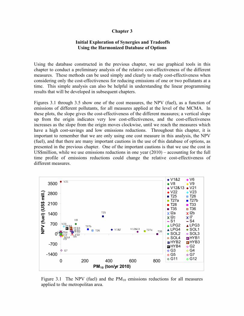
Chapter 3

Initial Exploration of Synergies and Tradeoffs Using the Harmonized Database of Options

Using the database constructed in the previous chapter, we use graphical tools in this chapter to conduct a preliminary analysis of the relative cost-effectiveness of the different measures. These methods can be used simply and clearly to study cost-effectiveness when considering only the cost-effectiveness for reducing emissions of one or two pollutants at a time. This simple analysis can also be helpful in understanding the linear programming results that will be developed in subsequent chapters. Figures 3.1 through 3.5 show one of the cost measures, the NPV (fuel), as a function of emissions of different pollutants, for all measures applied at the level of the MCMA. In these plots, the slope gives the cost-effectiveness of the different measures; a vertical slope up from the origin indicates very low cost-effectiveness, and the cost-effectiveness increases as the slope from the origin moves clockwise, until we reach the measures which have a high cost-savings and low emissions reductions. Throughout this chapter, it is important to remember that we are only using one cost measure in this analysis, the NPV (fuel), and that there are many important cautions in the use of this database of options, as presented in the previous chapter. One of the important cautions is that we use the cost in US$million, while we use emissions reductions in one year (2010) – accounting for the full time profile of emissions reductions could change the relative cost-effectiveness of different measures.

Figure 3.1 The NPV (fuel) and the PM10 emissions reductions for all measures applied to the metropolitan area.

V1&2

V8

V9

V12&13

V21

V22

V23

T25

T26 T27a

T27b

T35

I2b

LPG4

SOL4

HYB1HYB2

HYB3HYB4

G5

G7

G12

-1400

-700

0

700

1400

2100

2800

3500

0 200 400 600 800PM10 (ton/yr 2010)

NPV

(fue

l) (U

S$ m

ill.)

V1&2 V6V8 V9V12&13 V21V22 V23T25 T26T27a T27bT28 T33T35 T36I2a I2bI2c I7S1 S4LPG2 LPG3LPG4 SOL1SOL2 SOL3SOL4 HYB1HYB2 HYB3HYB4 G2G3 G4G5 G7G11 G12

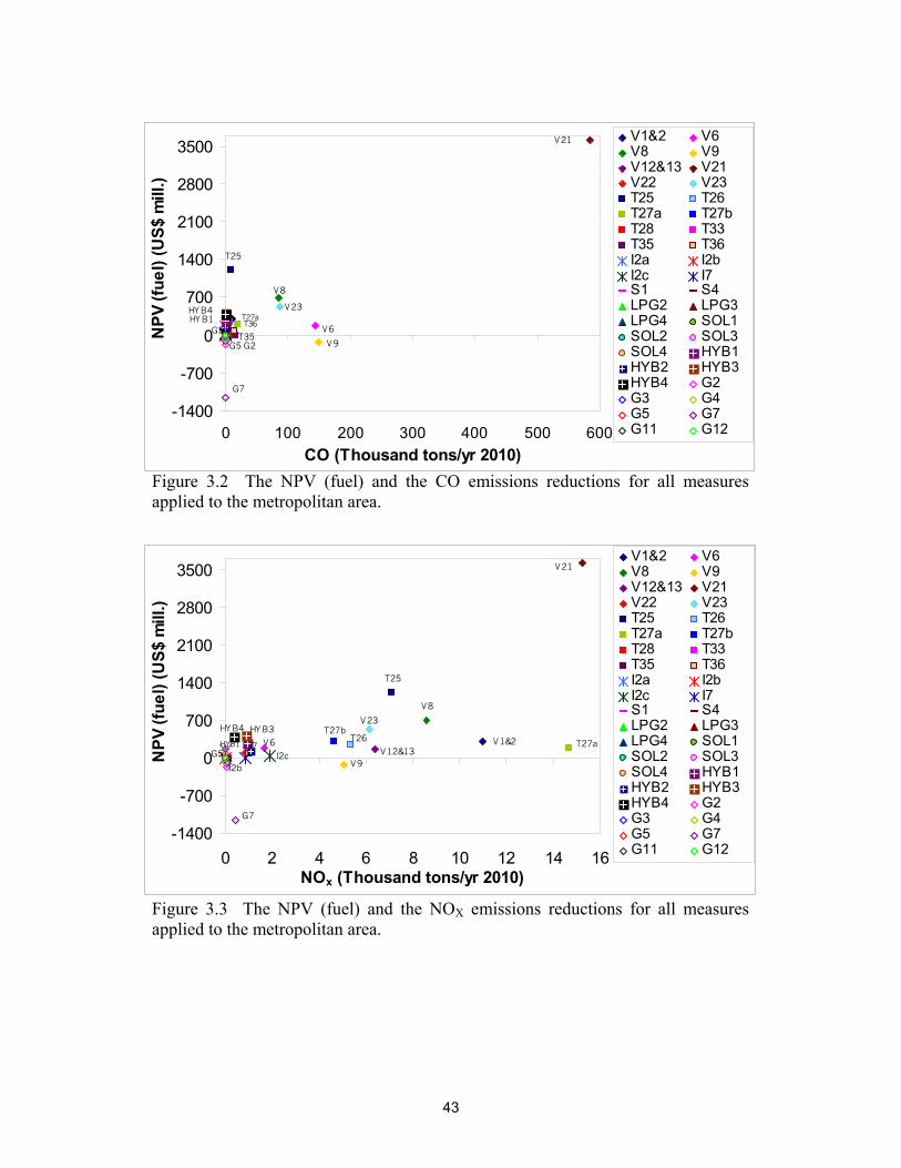
43

Figure 3.2 The NPV (fuel) and the CO emissions reductions for all measures applied to the metropolitan area.

Figure 3.3 The NPV (fuel) and the NOX emissions reductions for all measures applied to the metropolitan area.

V8

V9

V21

V23

T25

T35

T27aT36

G5 G2

HYB1

G7

HYB4

G5 V6

-1400

-700

0

700

1400

2100

2800

3500

0 100 200 300 400 500 600CO (Thousand tons/yr 2010)

NPV

(fue

l) (U

S$ m

ill.)

V1&2 V6V8 V9V12&13 V21V22 V23T25 T26T27a T27bT28 T33T35 T36I2a I2bI2c I7S1 S4LPG2 LPG3LPG4 SOL1SOL2 SOL3SOL4 HYB1HYB2 HYB3HYB4 G2G3 G4G5 G7G11 G12

V1&2

V8

V9V12&13

V21

V6

V23

T25

T26T27a

T27b

I2b

G7

HYB1

I2c

HYB3HYB4

G5I7

-1400

-700

0

700

1400

2100

2800

3500

0 2 4 6 8 10 12 14 16NOx (Thousand tons/yr 2010)

NPV

(fue

l) (U

S$ m

ill.)

V1&2 V6V8 V9V12&13 V21V22 V23T25 T26T27a T27bT28 T33T35 T36I2a I2bI2c I7S1 S4LPG2 LPG3LPG4 SOL1SOL2 SOL3SOL4 HYB1HYB2 HYB3HYB4 G2G3 G4G5 G7G11 G12

44

Figure 3.4 The NPV (fuel) and the HC emissions reductions for all measures applied to the metropolitan area.

Figure 3.5 The NPV (fuel) and the CO2 emissions reductions for all measures applied to the metropolitan area.

V 1 &2

V8

V9G2

V21

V23

T25

T27aT27b

T36

I2a

LPG4S1 S4

HYB4

G7

V6LPG3

-1400

-700

0

700

1400

2100

2800

3500

0 10 20 30 40 50 60HC (Thousand tons/yr 2010)

NPV

(fue

l) (U

S$ m

ill.)

V1&2 V6V8 V9V12&13 V21V22 V23T25 T26T27a T27bT28 T33T35 T36I2a I2bI2c I7S1 S4LPG2 LPG3LPG4 SOL1SOL2 SOL3SOL4 HYB1HYB2 HYB3HYB4 G2G3 G4G5 G7G11 G12

V1&2

V8

G2

V21

V23

T25

T26

T27a

G4G3

LPG4HYB1

HYB3HYB4

G5

G7

-1400

-700

0

700

1400

2100

2800

3500

-200 800 1,800 2,800 3,800CO2 (Thousand tons/yr 2010)

NPV

(fue

l) (U

S$ m

ill.)

V1&2 V6V8 V9V12&13 V21V22 V23T25 T26T27a T27bT28 T33T35 T36I2a I2bI2c I7S1 S4LPG2 LPG3LPG4 SOL1SOL2 SOL3SOL4 HYB1HYB2 HYB3HYB4 G2G3 G4G5 G7G11 G12

45

In addition to considering the cost-effectiveness of each pollutant individually, it is also possible to plot the cost-effectiveness for reductions of two pollutants simultaneously. Here, we calculate the cost-effectiveness of each measure for reducing each pollutant, by dividing the cost (here NPV (fuel)) by the emissions reduction, to obtain the cost-effectiveness as $/ton. The results from doing this division show a very wide range of numbers, which is not represented easily graphically. In place of showing these results, we rank the results from least cost-effective to most, which is more easily understood graphically. The results are shown in Figures 3.6 to 3.9, with the cost-effectiveness of each local pollutant compared with the cost-effectiveness of CO2 reductions, in order to analyze the local-global tradeoff or synergy. For all pollutants, measures which have no effect on emissions are shown here as having a rank of zero, being least cost-effective. In the case of CO2, some measures have a negative effect on emissions reductions, and these are shown as having a negative rank. In Figures 3.6 to 3.9, measures in the upper-right portion of the graph are most cost-effective for both pollutants, while those near the origin are less cost-effective for both pollutants. If all measures fall on a 1:1 line (up and to the right), this would indicate that there is no tradeoff between the pollutants – the best measures for one pollutant are also the best for the other pollutant. Deviations from a 1:1 line suggest that there are tradeoffs between emissions reductions for the two pollutants. A downward slope would indicate a complete tradeoff between the pollutants.

Figure 3.6 – Rank order cost-effectiveness for emissions reductions of PM10 and of CO2, using NPV (fuel) as the measure of cost, for all measures applied to the metropolitan area.

V1&2

V6

V8

V9

V12&13

V21

V22

V23

T25

T26

T27a

T27b

T28

T33

T35

T36

I2a I2b

I2c

I7

S1

S4

LPG2

LPG3

LPG4

SOL1SOL2

SOL3SOL4

HYB1

HYB2

HYB3

HYB4

G2

G3

G4

G5

G7

G11

G12

-5

0

5

10

15

20

25

30

35

0 5 10 15 20

Cost-effectiveness PM10

Cos

t-effe

ctiv

enes

s C

O2

V1&2 V6

V8 V9

V12&13 V21

V22 V23

T25 T26

T27a T27b

T28 T33

T35 T36

I2a I2b

I2c I7

S1 S4

LPG2 LPG3

LPG4 SOL1

SOL2 SOL3

SOL4 HYB1

HYB2 HYB3

HYB4 G2

G3 G4

G5 G7

G11 G12

MoreLess

Less

Mor

e

46

Figure 3.7 – Rank order cost-effectiveness for emissions reductions of CO and of CO2, using NPV (fuel) as the measure of cost, for all measures applied to the metropolitan area.

In general, Figures 3.6 to 3.9 show a strong relationship that the most cost-effective actions for individual air pollutants, are also the most cost-effective actions for emissions of CO2, when using NPV (fuel) as the measure of cost. This is particularly true for NOX. However, there are also important exceptions to this rule, including many measures that have no effect on emissions of one or more local pollutants, and some actions which may be good for reducing emissions of local pollutants, but have zero or negative emissions reductions for CO2. This is most notable for PM10, for which many measures have no effect on PM10, although they may produce benefits in terms of CO2 emissions reductions.

V1&2

V6

V8

V9

V12&13

V21

V22

V23

T25

T26

T27a

T27b

T28

T33

T35

T36

I2a

I2b

I2cI7

S1

S4

LPG2

LPG3

LPG4

SOL1SOL2

SOL3SOL4

HYB1

HYB2

HYB3

HYB4

G2

G3

G4

G5

G7

G11

G12

-5

0

5

10

15

20

25

30

35

0 5 10 15 20 25 30

Cost-effectiveness CO

Cos

t-effe

ctiv

enes

s C

O2

V1&2 V6

V8 V9

V12&13 V21

V22 V23

T25 T26

T27a T27b

T28 T33

T35 T36

I2a I2b

I2c I7

S1 S4

LPG2 LPG3

LPG4 SOL1

SOL2 SOL3

SOL4 HYB1

HYB2 HYB3

HYB4 G2

G3 G4

G5 G7

G11 G12

MoreLess

Less

Mor

e

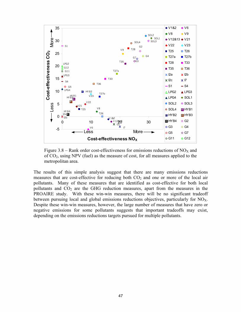
47

Figure 3.8 – Rank order cost-effectiveness for emissions reductions of NOX and of CO2, using NPV (fuel) as the measure of cost, for all measures applied to the metropolitan area.

The results of this simple analysis suggest that there are many emissions reductions measures that are cost-effective for reducing both CO2 and one or more of the local air pollutants. Many of these measures that are identified as cost-effective for both local pollutants and CO2 are the GHG reduction measures, apart from the measures in the PROAIRE study. With these win-win measures, there will be no significant tradeoff between pursuing local and global emissions reductions objectives, particularly for NOX. Despite these win-win measures, however, the large number of measures that have zero or negative emissions for some pollutants suggests that important tradeoffs may exist, depending on the emissions reductions targets pursued for multiple pollutants.

V1&2

V6

V8

V9

V12&13

V21

V22

V23

T25

T26

T27a

T27b

T28

T33

T35

T36

I2a

I2b

I2cI7

S1

S4

LPG2

LPG3

LPG4

SOL1SOL2

SOL3SOL4

HYB1

HYB2

HYB3

HYB4

G2

G3

G4

G5

G7

G11

G12

-5

0

5

10

15

20

25

30

35

0 10 20 30

Cost-effectiveness NOX

Cos

t-effe

ctiv

enes

s C

O2

V1&2 V6

V8 V9

V12&13 V21

V22 V23

T25 T26

T27a T27b

T28 T33

T35 T36

I2a I2b

I2c I7

S1 S4

LPG2 LPG3

LPG4 SOL1

SOL2 SOL3

SOL4 HYB1

HYB2 HYB3

HYB4 G2

G3 G4

G5 G7

G11 G12

MoreLess

Less

Mor

e

48

Figure 3.9 – Rank order cost-effectiveness for emissions reductions of HC and of CO2, using NPV (fuel) as the measure of cost, for all measures applied to the metropolitan area.

It is important to remember that the graphical representations of cost-effectiveness shown in this chapter have all used the NPV (fuel) as a measure of cost. The same analysis could be repeated using other cost measures, particularly the total investment cost. In Figures 3.10 and 3.11, we consider the relationship between the two cost measures – the NPV (fuel) and the total investment cost. The results show that there is a fairly close relationship between the two cost measures for the majority of measures, indicating that high costs using one indicator tend to correspond with high costs for the other cost measure. The exceptions are notable for the GHG control measures which were not included in PROAIRE. Several of these measures have a negative NPV (fuel) and so deviate from the close relationship seen for the other measures. This observation will be important for the results obtained when we apply the linear program.

V1&2

V6

V8

V9

V12&13

V21

V22

V23

T25

T26

T27a

T27b

T28

T33

T35

T36

I2a

I2b

I2cI7

S1

S4

LPG2

LPG3

LPG4

SOL1SOL2

SOL3SOL4

HYB1

HYB2

HYB3

HYB4

G2

G3

G4

G5

G7

G11

G12

-5

0

5

10

15

20

25

30

35

0 5 10 15 20 25 30

Cost-effectiveness HC

Cos

t-effe

ctiv

enes

s C

O2

V1&2 V6

V8 V9

V12&13 V21

V22 V23

T25 T26

T27a T27b

T28 T33

T35 T36

I2a I2b

I2c I7

S1 S4

LPG2 LPG3

LPG4 SOL1

SOL2 SOL3

SOL4 HYB1

HYB2 HYB3

HYB4 G2

G3 G4

G5 G7

G11 G12

MoreLess

Less

Mor

e

49

Figure 3.10 – Total investment costs and NPV (fuel) for all measures applied to the metropolitan area.

V1&2

V8

V9

V21

V23

T25

T26T27a

T27b

HYB3

G2G3

G7

-1400

-700

0

700

1400

2100

2800

3500

0 2000 4000 6000 8000 10000

Total Investment ($US)

NPV

(fue

l) ($

US)

V1&2 V6

V8 V9

V12&13 V21

V22 V23

T25 T26

T27a T27b

T28 T33

T35 T36

I2a I2b

I2c I7

S1 S4

LPG2 LPG3

LPG4 SOL1

SOL2 SOL3

SOL4 HYB1

HYB2 HYB3

HYB4 G2

G3 G4

G5 G7

G11 G12

50

Figure 3.11 – Detail of Figure 3.10.

V1&2

V6

V8

V9

V12&13

V21

V22

V23

T25

T26

T27a

T27b

T35

T36

I2a

I2c

SOL3

HYB1

HYB2

HYB3

HYB4

G2G3

G4

G5

-200

0

200

400

600

0 500 1000 1500

Total Investment ($US)

NPV

(fue

l) ($

US)

V1&2 V6

V8 V9

V12&13 V21

V22 V23

T25 T26

T27a T27b

T28 T33

T35 T36

I2a I2b

I2c I7

S1 S4

LPG2 LPG3

LPG4 SOL1

SOL2 SOL3

SOL4 HYB1

HYB2 HYB3

HYB4 G2

G3 G4

G5 G7

G11 G12

51

Chapter 4

Development of a Linear Programming Model for Analyzing Co-Control In the previous chapter, we presented some illustrative methods of considering the tradeoffs in cost between the goals of reducing emissions of urban air pollutants and reducing emissions of GHGs. While it is possible to draw meaningful conclusions from these methods, these methods are incapable of addressing cost-effectiveness for more than two pollutants at a time. A linear program (LP), on the other hand, can be useful in finding a least-cost set of options when more than two pollutants are simultaneously considered. An LP can be thought of not so much as a model, but more accurately as a search tool, which can efficiently search through all combinations of options to find an optimal solution under given constraints. Instead of iteratively trying different options to try to find a good solution, a decision analyst can use an LP to directly find the optimal choice, and can then consider the features of this combination of options that make this the optimal. In our case, the LP will be formulated to minimize the total cost of the emissions control program, subject to constraints on the emissions reductions chosen for many different pollutants. As discussed in the first chapter of this report, the main goals of developing and employing an LP for Mexico City are:

1) To develop a tool that will be useful for CAM in evaluating different emissions control measures, and therefore aid in decision-making.

2) To use the LP to explore the relationships (tradeoffs or synergies) between the different goals of urban air pollution control and mitigation of GHG emissions.

Regarding the first goal, it is important to remember that the LP is a way of efficiently finding the minimum cost solution, and that the solution of the LP is not necessarily the best policy. Rather, there will be other important qualitative factors to be taken into consideration in evaluating a best plan for emissions reductions. Some humility is therefore required in interpreting the results of this study. Still, the LP can be very useful in allowing quantitative exploration of how different targets can be met most cost-effectively. Rather than providing a single answer, we suggest that for use in designing an integrated air quality and GHG emissions plan, that the LP be used in an iterative manner. Which emissions reductions measures are consistently included in the least-cost solution? How do the total costs change as the targets for different pollutants are changed, and how can we use that information to decide on cost-effective emissions control targets? The LP results are therefore intended more as a foundation for further policy discussions, rather than being the best policy solution. Regarding the second goal, we would like to be able to decide the best policies for a range of emissions reductions targets for different pollutants, and then consider how those sets of policies differ as the emissions reductions targets change. Such a goal is impractical in the simple sense that many factors, both quantifiable and qualitative, need to be considered in developing good policies. Therefore, determining the best policy is partly subjective.

52

Instead of determining the best policies for each set of emissions reductions targets, we will consider the least-cost set of actions as a useful surrogate for the “best” set of policies. While this leaves out consideration of qualitative factors that are important for decisions, it allows a greater flexibility in seeing how preferred policies and total costs change in an integrated way, as the emission reduction targets change. In the next section, we present the formulation of the LP for use in this study. Following that, we highlight the important assumptions of the LP. Note that Microsoft Excel is used in this study, as a platform for conveniently developing and solving the LP. A guide to running the LP in Microsoft Excel is included as Appendix C of this report. 4.1 Formulation of a LP Model for the Co-control urban air pollutants and GHGs Stated in words, the LP model is formulated as:

Minimize ... the total cost of implementing a pollution control program, by changing ... the activity levels of the different control options, subject to constraints on ... the maximum (and minimum) activity level for each

control option, ... and the minimum allowable emissions reduction for each pollutant.

Mathematically, this can be expressed as:

Minimize: Cost = ∑=

n

iiiCA

1

)(

Subject to: ( )maxii AA ≤ for ni ...1= 0≥iA for ni ...1=

∑=

≥n

ikkii TEA

1, )( for max...1 kk =

where Ai is the activity level of pollution control measure i; Ci is the unit cost of implementing measure i; n is the number of pollution control measures considered; Ei,k is the unit emissions reduction of pollutant k due to implementation of pollution control measure i; (Ai)max is the maximum activity level allowable for measure i; Tk is the minimum allowable total emissions for pollutant k (the emissions reduction target); and kmax is the number of pollutants considered. The Tk values are the emissions constraints the user will select, and can be varied to explore a range of emissions reduction constraints. The unit costs and unit emission reductions can also be varied as new information comes available, or to explore the sensitivity to these emission reductions. Note that in order to use an LP, it is necessary that the objective function and all of the constraints are linear functions – in the formulation shown above, we see that this is indeed

53

the case. An LP algorithm therefore can be expected to efficiently find the optimal solution to this problem every time that it is run, as long as the constraints do not prevent a feasible solution. For example, if an emissions reduction target is too large, it may not be possible to get such a large reduction using the available measures, and the LP will not yield a feasible solution. Note also that the LP algorithm can be expected to yield the optimal result each time it is run, regardless of the initial conditions. As discussed in the Chapter 2, we have defined several measures of cost that could be used in the objective function of this study: the public investment cost, the private investment cost, the total investment cost (the sum of public and private), and the NPV (fuel). Of these, we will use the total investment cost and the NPV (fuel) as alternative objective functions in this study. The activity levels can be defined in any way for any measure, as long as the unit emissions reductions (unit cost) at the reference activity level times the maximum activity level gives the true maximum level implementation for each measure. As discussed in Chapter 2, we have decided to define the activity levels of the PROAIRE measures such as an activity level of 1.0 indicates the level of implementation proposed in PROAIRE. Most GHG mitigation measures are defined such that their maximum activity levels are 1.0, except for the solar water heating measures, which are defined relative to a pilot project. An additional constraint is also required for the measures that replace the fleet of RTP (publicly-owned) buses, since measure V22 and the four hybrid electric bus measures are each modeled to replace the entire RTP fleet. This constraint can be expressed as: the sum of the activity levels for these five measures must be less than or equal to 1.0. The LP could select to use one of these measures, none of these measures, or any combination of the fractional implementation of each measure such that the sum of activity levels is less than 1.0. These are the only measures for which such an extra constraint is necessary. Other formulations of the LP are also possible. We could, for example, minimize the NPV (fuel) while adding a constraint on the investment costs, to reflect a hard budget constraint. We could also maximize the emissions reductions of one pollutant or a weighted sum of different pollutants, subject to constraints on the cost. The minimum activity level could likewise be increased from zero to some larger value, reflecting that a certain level of implementation of a particular measure is necessary. While these formulations of the problem may be useful as alternatives to help inform decisions, we do not develop these approaches here. We suggest that in future work, it will be important to work together with decision makers and stakeholders to develop the LP such that it reflects better the way these actors conceive of the decision making problem. 4.2 Key Assumptions in Applying the LP A number of assumptions are implicitly built into the LP. One is that the decision-maker is faced with making decisions now, concerning the implementation of a pollution control program over the 2002-2010 time horizon. The analysis is therefore static and does not include possibilities of changing the timing of different control options, or of learning from the (successful or unsuccessful) implementation of control measures. The use of an LP in a dynamic framework could allow for decisions to be made and optimized dynamically

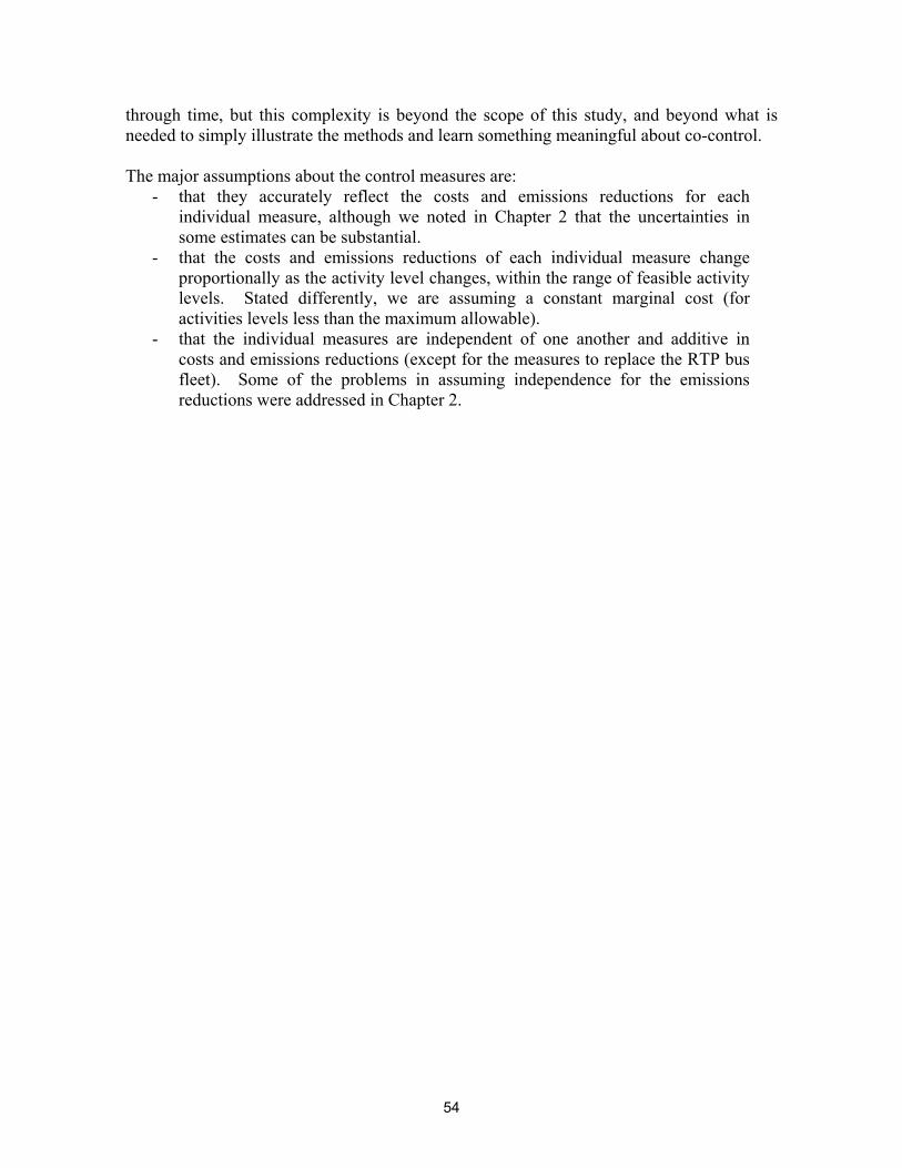
54

through time, but this complexity is beyond the scope of this study, and beyond what is needed to simply illustrate the methods and learn something meaningful about co-control. The major assumptions about the control measures are:

- that they accurately reflect the costs and emissions reductions for each individual measure, although we noted in Chapter 2 that the uncertainties in some estimates can be substantial.

- that the costs and emissions reductions of each individual measure change proportionally as the activity level changes, within the range of feasible activity levels. Stated differently, we are assuming a constant marginal cost (for activities levels less than the maximum allowable).

- that the individual measures are independent of one another and additive in costs and emissions reductions (except for the measures to replace the RTP bus fleet). Some of the problems in assuming independence for the emissions reductions were addressed in Chapter 2.

55

Chapter 5

Analysis of the Co-Control of Urban Air Pollutants and Greenhouse Gases 5.1 Meeting the local emissions reductions totals in PROAIRE 5.1.1 Illustration of LP Before considering constraints on emissions reductions for CO2, we first use the LP to meet the emissions reductions targets in PROAIRE using only the PROAIRE measures. We do this to consider whether there may be potential to increase the investment in more cost-effective measures in PROAIRE, and to reduce the investment in less cost-effective measures, in order to achieve a more cost-effective air quality control plan. In the LP, we do this by minimizing either the investment cost or the NPV (fuel), and placing constraints on the emissions reductions of each pollutant. The emission reduction constraints are set equal to the estimates of the total emissions reductions of PROAIRE, using the emissions reduction and cost estimates in this study (Table 2.4). To illustrate the LP, the first case we consider is where we use the LP to find the combination of options that minimizes the NPV (fuel). This is illustrated in Figure 5.1. Figure 5.1a shows the activity levels of the PROAIRE measures – we have defined the activity levels in PROAIRE to be 1.0 for all measures. For each measure, we have also defined the maximum activity level in Table 2.1, and these are also shown in this Figure. Our task then is to find some combinations of options that meet the same emissions reductions as in PROAIRE at a lower cost, while the activity levels of each measure remain less than (or equal to) the maximum activity levels. If we were to do this ourselves, we might start by increasing the activity level of the measure we think is most cost-effective for some pollutant, while decreasing the activity level of another measure we think is least cost-effective, such that there is no net change in emissions at a lower cost (here the NPV (fuel)). We could continue trying solutions in this manner, but with many options and with many pollutants to consider at the same time, we would run into a very complex situation very quickly. The LP simply allows us to arrive at the very best (minimum NPV (fuel)) solution very efficiently. For this first example, the combination of activity levels that gives the minimum NPV (fuel) is shown in Figure 5.1b. Here we see that in this optimal solution, the activity levels of many measures are at their maximum levels, while four measures are no longer included in the optimal solution. Normally, this is what the LP will do – find the more cost-effective measures and suggest doing as much of those measures as possible, while omitting the least cost-effective measures from the solution set. Several measures are given activity levels between zero and their maximum levels – these measures are “marginal” actions, indicating that their cost-effectiveness is probably intermediate, and that if we were to change the emissions reduction targets slightly, it is likely that the activity levels of these measures would change slightly.

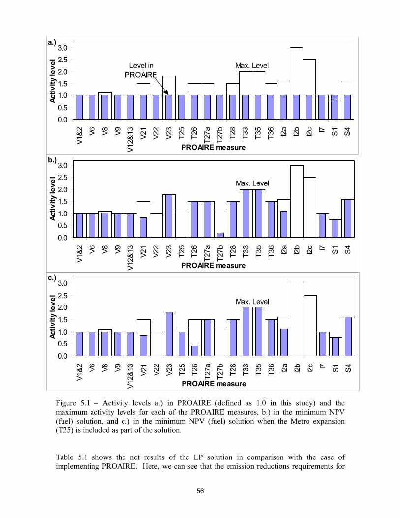
56

Figure 5.1 – Activity levels a.) in PROAIRE (defined as 1.0 in this study) and the maximum activity levels for each of the PROAIRE measures, b.) in the minimum NPV (fuel) solution, and c.) in the minimum NPV (fuel) solution when the Metro expansion (T25) is included as part of the solution. Table 5.1 shows the net results of the LP solution in comparison with the case of implementing PROAIRE. Here, we can see that the emission reductions requirements for

0.00.51.01.52.02.53.0

V1&2

V6

V8

V9

V12&

13

V21

V22

V23

T25

T26

T27a

T27b

T28

T33

T35

T36

I2a

I2b

I2c I7

S1

S4

PROAIRE measure

Activ

ity le

vel

Max. LevelLevel inPROAIRE

a.)

0.00.51.01.52.02.53.0

V1&2

V6

V8

V9

V12&

13

V21

V22

V23

T25

T26

T27a

T27b

T28

T33

T35

T36

I2a

I2b

I2c I7

S1

S4

PROAIRE measure

Activ

ity le

vel

Max. Level

b.)

0.00.51.01.52.02.53.0

V1&2

V6

V8

V9

V12&

13

V21

V22

V23

T25

T26

T27a

T27b

T28

T33

T35

T36

I2a

I2b

I2c I7

S1

S4

PROAIRE measure

Activ

ity le

vel

Max. Level

c.)

57

all five local pollutants (set at PROAIRE levels) were met in the LP solution, and that the PM10 emissions reduction actually exceeded the PROAIRE solution. This was a fortunate outcome that indicates that the least-cost solution found when minimizing for the four other pollutants already had high emissions reductions for PM10 – no solution with a lower cost exists with less PM10 emissions reductions. In this case, we say that the constraint on PM10 emissions is “not a binding constraint” since it did not affect the best solution. Table 5.1 also shows that all of the measures of cost decreased relative to PROAIRE. Certainly the NPV (fuel) should have decreased since that was the objective function that was minimized – the fact that the other cost measures also decreased reflects that when the NPV (fuel) is high, the investment costs are generally also high (see Figure 3.10). Table 5.1 – Costs and emissions reductions under PROAIRE (for 22 measures, using data from this study), and in the minimum NPV (fuel) solution. Also shown are shadow prices for pollutant reduction constraints from the minimum NPV (fuel) solution. Costs are in US$million, emissions reductions are in tonnes/yr in 2010 and shadow prices are US$/(tonne/yr in 2010).

PROAIRE Minimum NPV (fuel) solution

Shadow prices of Min.

MPV (fuel)

Min. NPV (fuel) with Metro (T25)

in solution Public investment 9,934 6,286 8,837 Private investment 13,025 12,929 12,949 Total investment 22,959 19,216 21,786 NPV (fuel) 7,656 6,168 7,039 PM10 3,767 4,355 0 4,365 SO2 627 627 3,019,951 627 CO 1,138,167 1,138,167 3,909 1,138,167 NOX 90,698 90,698 14,965 90,698 HC 137,259 137,259 20,021 137,259 CO2 2,246,946 2,614,201 2,731,086

It is also interesting to note that measure I2b (industrial PM10 controls) is not included in the optimal solution, although it is in fact a very cost-effective way of reducing PM10. The reason that it was not included is because PM10 is not a binding constraint in this scenario – we already exceed the target emissions reductions for PM10, and investing to control more PM10 will only increase the total cost. For this reason, the results of the LP do not always indicate cost-effectiveness for measures that control only one or two pollutants, but should indicate cost-effectiveness for cases where a measure affects multiple pollutants. Table 5.1 also shows the shadow prices of the solution for the different pollutant constraints. In this problem, the shadow price is defined as the increase in cost (here, NPV (fuel)) for an increase in the required emissions reduction (the emissions constraint) of one tonne per year in 2010. (Alternatively, it is the decrease in the NPV (fuel) for a one tonne per year decrease in the emissions constraint.) The units of the shadow price are therefore US$/(tonne/yr) – these values should therefore not be used to compare against control costs

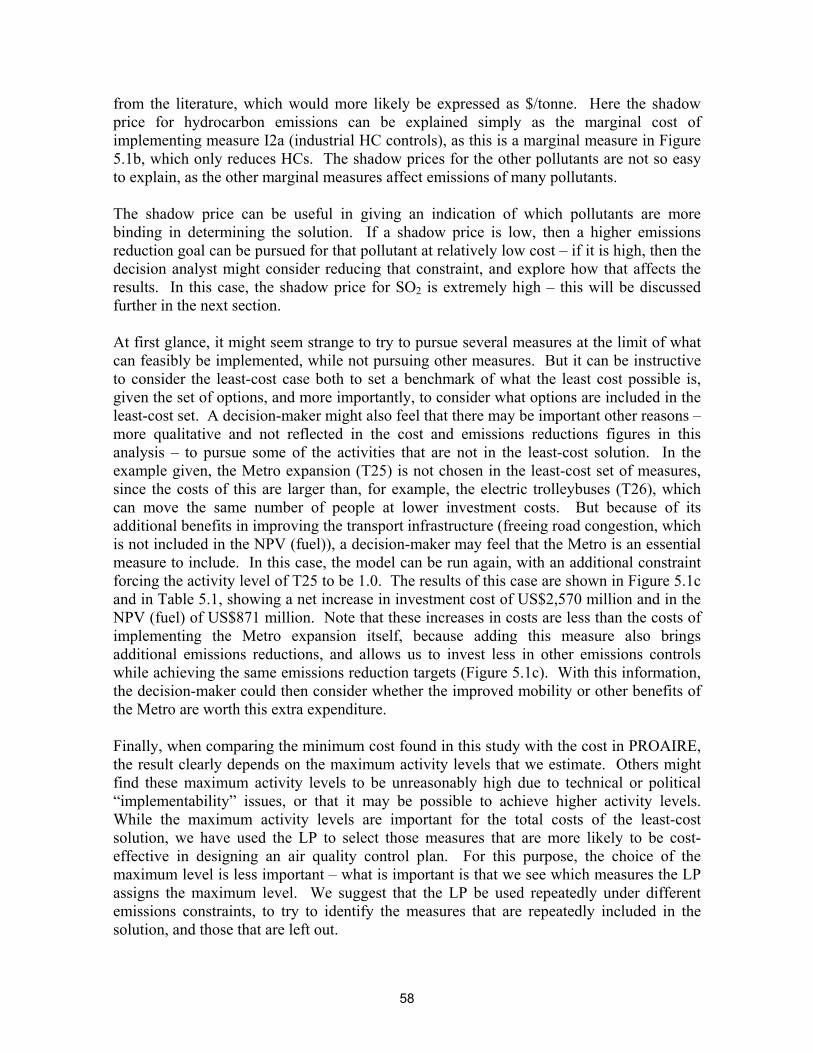
58

from the literature, which would more likely be expressed as $/tonne. Here the shadow price for hydrocarbon emissions can be explained simply as the marginal cost of implementing measure I2a (industrial HC controls), as this is a marginal measure in Figure 5.1b, which only reduces HCs. The shadow prices for the other pollutants are not so easy to explain, as the other marginal measures affect emissions of many pollutants. The shadow price can be useful in giving an indication of which pollutants are more binding in determining the solution. If a shadow price is low, then a higher emissions reduction goal can be pursued for that pollutant at relatively low cost – if it is high, then the decision analyst might consider reducing that constraint, and explore how that affects the results. In this case, the shadow price for SO2 is extremely high – this will be discussed further in the next section. At first glance, it might seem strange to try to pursue several measures at the limit of what can feasibly be implemented, while not pursuing other measures. But it can be instructive to consider the least-cost case both to set a benchmark of what the least cost possible is, given the set of options, and more importantly, to consider what options are included in the least-cost set. A decision-maker might also feel that there may be important other reasons – more qualitative and not reflected in the cost and emissions reductions figures in this analysis – to pursue some of the activities that are not in the least-cost solution. In the example given, the Metro expansion (T25) is not chosen in the least-cost set of measures, since the costs of this are larger than, for example, the electric trolleybuses (T26), which can move the same number of people at lower investment costs. But because of its additional benefits in improving the transport infrastructure (freeing road congestion, which is not included in the NPV (fuel)), a decision-maker may feel that the Metro is an essential measure to include. In this case, the model can be run again, with an additional constraint forcing the activity level of T25 to be 1.0. The results of this case are shown in Figure 5.1c and in Table 5.1, showing a net increase in investment cost of US$2,570 million and in the NPV (fuel) of US$871 million. Note that these increases in costs are less than the costs of implementing the Metro expansion itself, because adding this measure also brings additional emissions reductions, and allows us to invest less in other emissions controls while achieving the same emissions reduction targets (Figure 5.1c). With this information, the decision-maker could then consider whether the improved mobility or other benefits of the Metro are worth this extra expenditure. Finally, when comparing the minimum cost found in this study with the cost in PROAIRE, the result clearly depends on the maximum activity levels that we estimate. Others might find these maximum activity levels to be unreasonably high due to technical or political “implementability” issues, or that it may be possible to achieve higher activity levels. While the maximum activity levels are important for the total costs of the least-cost solution, we have used the LP to select those measures that are more likely to be cost-effective in designing an air quality control plan. For this purpose, the choice of the maximum level is less important – what is important is that we see which measures the LP assigns the maximum level. We suggest that the LP be used repeatedly under different emissions constraints, to try to identify the measures that are repeatedly included in the solution, and those that are left out.

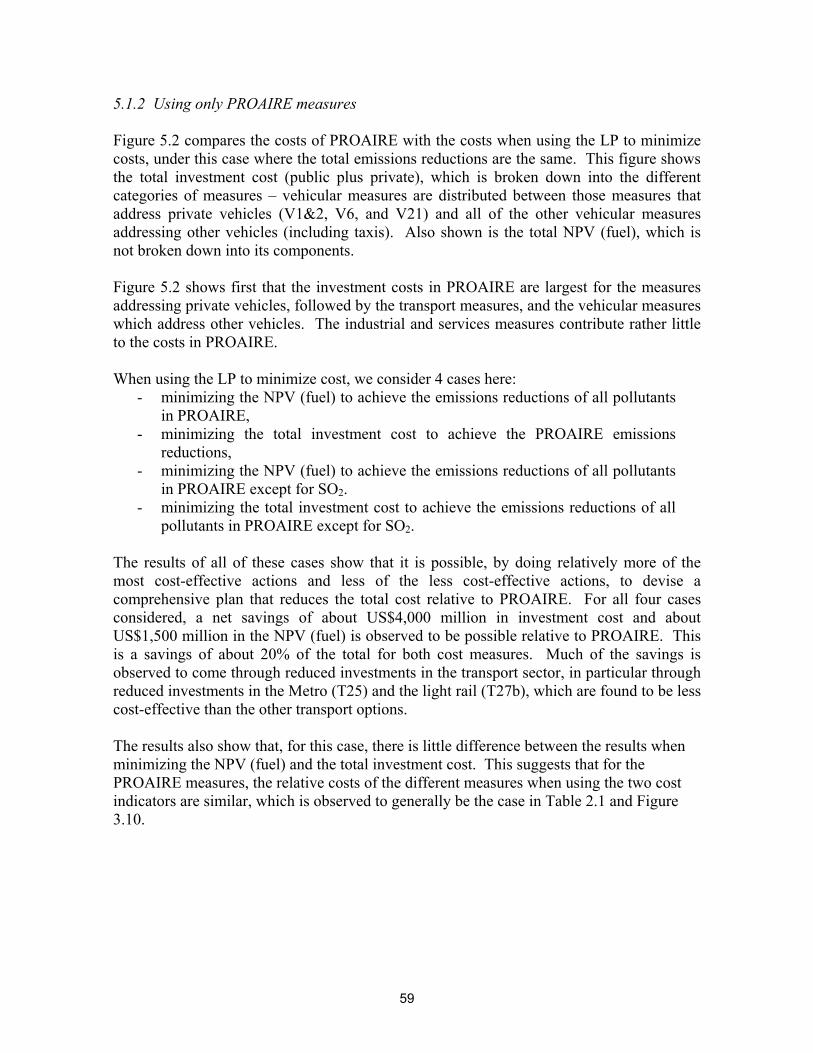
59

5.1.2 Using only PROAIRE measures Figure 5.2 compares the costs of PROAIRE with the costs when using the LP to minimize costs, under this case where the total emissions reductions are the same. This figure shows the total investment cost (public plus private), which is broken down into the different categories of measures – vehicular measures are distributed between those measures that address private vehicles (V1&2, V6, and V21) and all of the other vehicular measures addressing other vehicles (including taxis). Also shown is the total NPV (fuel), which is not broken down into its components. Figure 5.2 shows first that the investment costs in PROAIRE are largest for the measures addressing private vehicles, followed by the transport measures, and the vehicular measures which address other vehicles. The industrial and services measures contribute rather little to the costs in PROAIRE. When using the LP to minimize cost, we consider 4 cases here:

- minimizing the NPV (fuel) to achieve the emissions reductions of all pollutants in PROAIRE,

- minimizing the total investment cost to achieve the PROAIRE emissions reductions,

- minimizing the NPV (fuel) to achieve the emissions reductions of all pollutants in PROAIRE except for SO2.

- minimizing the total investment cost to achieve the emissions reductions of all pollutants in PROAIRE except for SO2.

The results of all of these cases show that it is possible, by doing relatively more of the most cost-effective actions and less of the less cost-effective actions, to devise a comprehensive plan that reduces the total cost relative to PROAIRE. For all four cases considered, a net savings of about US$4,000 million in investment cost and about US$1,500 million in the NPV (fuel) is observed to be possible relative to PROAIRE. This is a savings of about 20% of the total for both cost measures. Much of the savings is observed to come through reduced investments in the transport sector, in particular through reduced investments in the Metro (T25) and the light rail (T27b), which are found to be less cost-effective than the other transport options. The results also show that, for this case, there is little difference between the results when minimizing the NPV (fuel) and the total investment cost. This suggests that for the PROAIRE measures, the relative costs of the different measures when using the two cost indicators are similar, which is observed to generally be the case in Table 2.1 and Figure 3.10.

60

Figure 5.2 – Total costs of investment and NPV (fuel) for the measures in PROAIRE, and when minimizing cost (NPV (fuel) or total investment) to achieve the emissions reductions in PROAIRE. Also presented is the case where no constraint on SO2 emissions is considered.

Figure 5.3 – Total costs of investment and NPV (fuel) for the measures in PROAIRE, and when minimizing cost (NPV (fuel) or total investment) to achieve the emissions reductions in PROAIRE (except for SO2) – using only the measures in PROAIRE (as in Figure 5.2), and when adding other GHG measures.

0

5,000

10,000

15,000

20,000

25,000

PROAIRE Min. NPV(fuel)

Min.Invest.Total

Min. NPV(fuel)

Min.Invest.Total

Tota

l Inv

estm

ent (

US$

mill

ion)

GHG measuresServicesIndustryTransportOther vehiclesPrivate vehicles

NPV (fuel)

PROAIRE measures only

Including other GHG measures

0

5,000

10,000

15,000

20,000

25,000

PROAIRE Min. NPV(fuel)

Min.Invest.Total

Min. NPV(fuel)

Min.Invest.Total

Tota

l Inv

estm

ent (

US$

mill

ion)

ServicesIndustryTransportOther vehiclesPrivate vehiclesNPV (fuel)

PROAIRE emissions PROAIRE emissions

except SO2

61

Finally, the results also show some additional cost savings when the emissions reduction constraint for SO2 is removed. We chose to consider this case because the total emissions reductions of SO2 from this set of PROAIRE measures is small (2% of the total SO2 emissions in 2010), and because emissions reductions of SO2 were not estimated as carefully as for other pollutants, and were not estimated for several measures which likely have some effect on SO2. Further, the findings in Table 5.1 suggested that the shadow price of SO2 is very large. The requirement to meet SO2 targets, with few measures to choose from, forces the LP to higher-cost solutions, which do not have a significant air quality benefit. For this reason, we will, through the remainder of this study, focus on emissions reductions targets for the other four criteria pollutants and omit the constraint for SO2. 5.1.3. Including other local measures Next we consider whether the total costs of achieving the PROAIRE emissions reductions can be reduced by including the other emissions reductions measures that we included in Table 2.1, which were not included in PROAIRE. We do not consider here the GHG mitigation measures applied outside of the MCMA (in Table 2.2), since these measures have no effect on emissions of local contaminants. These measures will be added later when we consider adding targets for CO2 emissions. Figure 5.3 again shows PROAIRE and the minimum cost solutions found when meeting the PROAIRE emissions reductions totals (except for SO2), and then considers the effects of allowing emissions reductions to come from the other local measures, named here as “GHG measures.” The results show that when minimizing the total investment, there is very little difference from when only PROAIRE measures were considered. In this case, the only change relative to using only PROAIRE measures comes from including two different measures to reduce residential emissions of LPG (LPG2 and LPG3), while reducing the investment in industrial controls of hydrocarbons (I2a) and the PROAIRE measure to reduce residential LPG emissions (S4). When minimizing for the NPV (fuel), however, the effect of including the GHG measures is seen to decrease the total NPV (fuel) substantially, by about US$2,300 million. Meanwhile, this same solution increases the total investment cost substantially, by about US$1,500 million. This solution decreases the NPV (fuel) by including all of the GHG measures which have a negative NPV (fuel) – LPG2, all of the solar water heater measures, and G2, G3, G4, and G7. Meanwhile less investment is now needed in some of the PROAIRE measures, due to the reductions in emissions of local pollutants that come from the GHG measures. These findings show that while the GHG measures chosen by the LP have a negative NPV (fuel) (are cost-saving measures in net), they often have a large investment cost. From Table 2.1 and Figure 3.10, we see that this is often the case for these measures, as many have large up-front investments, which could be a barrier to their implementation, but significant savings of fuel and electricity consumption during their lifetimes.

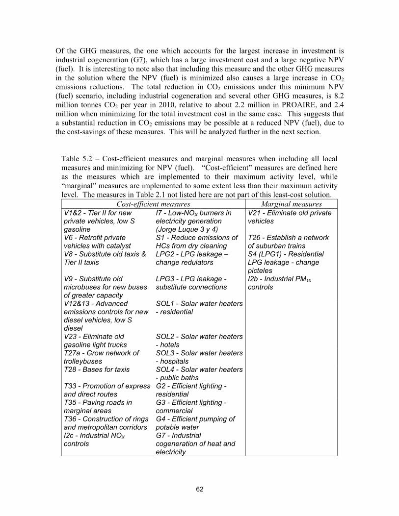
62

Of the GHG measures, the one which accounts for the largest increase in investment is industrial cogeneration (G7), which has a large investment cost and a large negative NPV (fuel). It is interesting to note also that including this measure and the other GHG measures in the solution where the NPV (fuel) is minimized also causes a large increase in CO2 emissions reductions. The total reduction in CO2 emissions under this minimum NPV (fuel) scenario, including industrial cogeneration and several other GHG measures, is 8.2 million tonnes CO2 per year in 2010, relative to about 2.2 million in PROAIRE, and 2.4 million when minimizing for the total investment cost in the same case. This suggests that a substantial reduction in CO2 emissions may be possible at a reduced NPV (fuel), due to the cost-savings of these measures. This will be analyzed further in the next section.

Table 5.2 – Cost-efficient measures and marginal measures when including all local measures and minimizing for NPV (fuel). “Cost-efficient” measures are defined here as the measures which are implemented to their maximum activity level, while “marginal” measures are implemented to some extent less than their maximum activity level. The measures in Table 2.1 not listed here are not part of this least-cost solution.

Cost-efficient measures Marginal measures V1&2 - Tier II for new private vehicles, low S gasoline

I7 - Low-NOX burners in electricity generation (Jorge Luque 3 y 4)

V21 - Eliminate old private vehicles

V6 - Retrofit private vehicles with catalyst

S1 - Reduce emissions of HCs from dry cleaning

T26 - Establish a network of suburban trains

V8 - Substitute old taxis & Tier II taxis

LPG2 - LPG leakage – change redulators

S4 (LPG1) - Residential LPG leakage - change picteles

V9 - Substitute old microbuses for new buses of greater capacity

LPG3 - LPG leakage - substitute connections

I2b - Industrial PM10 controls

V12&13 - Advanced emissions controls for new diesel vehicles, low S diesel

SOL1 - Solar water heaters - residential

V23 - Eliminate old gasoline light trucks

SOL2 - Solar water heaters - hotels

T27a - Grow network of trolleybuses

SOL3 - Solar water heaters - hospitals

T28 - Bases for taxis SOL4 - Solar water heaters - public baths

T33 - Promotion of express and direct routes

G2 - Efficient lighting - residential

T35 - Paving roads in marginal areas

G3 - Efficient lighting - commercial

T36 - Construction of rings and metropolitan corridors

G4 - Efficient pumping of potable water

I2c - Industrial NOX controls

G7 - Industrial cogeneration of heat and electricity

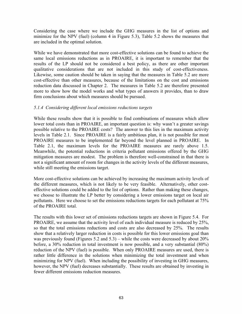
63

Considering the case where we include the GHG measures in the list of options and minimize for the NPV (fuel) (column 4 in Figure 5.3), Table 5.2 shows the measures that are included in the optimal solution. While we have demonstrated that more cost-effective solutions can be found to achieve the same local emissions reductions as in PROAIRE, it is important to remember that the results of the LP should not be considered a best policy, as there are other important qualitative considerations that are not included in this study of cost-effectiveness. Likewise, some caution should be taken in saying that the measures in Table 5.2 are more cost-effective than other measures, because of the limitations on the cost and emissions reduction data discussed in Chapter 2. The measures in Table 5.2 are therefore presented more to show how the model works and what types of answers it provides, than to draw firm conclusions about which measures should be pursued. 5.1.4 Considering different local emissions reductions targets While these results show that it is possible to find combinations of measures which allow lower total costs than in PROAIRE, an important question is: why wasn’t a greater savings possible relative to the PROAIRE costs? The answer to this lies in the maximum activity levels in Table 2.1. Since PROAIRE is a fairly ambitious plan, it is not possible for most PROAIRE measures to be implemented far beyond the level planned in PROAIRE. In Table 2.1, the maximum levels for the PROAIRE measures are rarely above 1.5. Meanwhile, the potential reductions in criteria pollutant emissions offered by the GHG mitigation measures are modest. The problem is therefore well-constrained in that there is not a significant amount of room for changes in the activity levels of the different measures, while still meeting the emissions target. More cost-effective solutions can be achieved by increasing the maximum activity levels of the different measures, which is not likely to be very feasible. Alternatively, other cost-effective solutions could be added to the list of options. Rather than making these changes, we choose to illustrate the LP better by considering a lower emissions target on local air pollutants. Here we choose to set the emissions reductions targets for each pollutant at 75% of the PROAIRE total. The results with this lower set of emissions reductions targets are shown in Figure 5.4. For PROAIRE, we assume that the activity level of each individual measure is reduced by 25%, so that the total emissions reductions and costs are also decreased by 25%. The results show that a relatively larger reduction in costs is possible for this lower emissions goal than was previously found (Figures 5.2 and 5.3) – while the costs were decreased by about 20% before, a 30% reduction in total investment is now possible, and a very substantial (80%) reduction of the NPV (fuel) is possible. When only PROAIRE measures are used, there is rather little difference in the solutions when minimizing the total investment and when minimizing for NPV (fuel). When including the possibility of investing in GHG measures, however, the NPV (fuel) decreases substantially. These results are obtained by investing in fewer different emissions reduction measures.

64

Figure 5.4 – 75% of the total costs of investment and NPV (fuel) for the measures in PROAIRE, and when minimizing cost (NPV (fuel) or total investment) to achieve 75% of the emissions reductions in PROAIRE (except for SO2) – using only the measures in PROAIRE, and when adding other GHG measures.

In general, therefore, these results show that where there is more flexibility in selecting the most cost-effective measures, the LP can be more valuable in decreasing total costs. Results when varying constraints like this can help prioritize the more cost-effective measures, by studying which measures are repeatedly included in the solutions. 5.1.5 Exploring variations in emission reduction targets of individual emissions Other experiments using the LP can be useful in informing policy decisions. Here we vary the emissions targets for one pollutant while constraining the model to achieve the PROAIRE targets for the other pollutants, and consider how the total cost changes. This experiment can be useful in setting emissions targets for the different pollutants – if the costs increase sharply at one point, the target might be set below this increase. For illustration, we use the case where we use PROAIRE emissions targets, we consider all local control measures (including GHG measures), and we minimize for the NPV (fuel). In Figure 5.5, we force the LP to meet PROAIRE emissions reduction goals for HCs, PM10, and CO, but vary the NOX emissions reduction goal. In this manner, we can see the relative costs of NOX emissions reductions, evaluated incrementally to PROAIRE emissions reduction goals, rather than evaluating NOX emissions reduction costs directly. Figure 5.5 shows the total investment cost of PROAIRE and the NPV (fuel) cost of PROAIRE. Point B in Figure 5.5 shows the costs of the minimum NPV (fuel) solution presented in Figure 5.3. Then costs are shown over a range of NOX emissions reduction targets. At the high end of NOX emissions reductions we approach the maximum NOX

0

2,000

4,000

6,000

8,000

10,000

12,000

14,000

16,000

18,000

PROAIRE Min. NPV(fuel)

Min.Invest.Total

Min. NPV(fuel)

Min.Invest.Total

Tota

l Inv

estm

ent (

US$

mill

ion)

GHG measuresServicesIndustryTransportOther vehiclesPrivate vehiclesNPV (fuel)

PROAIRE measures only

Including other GHG measures

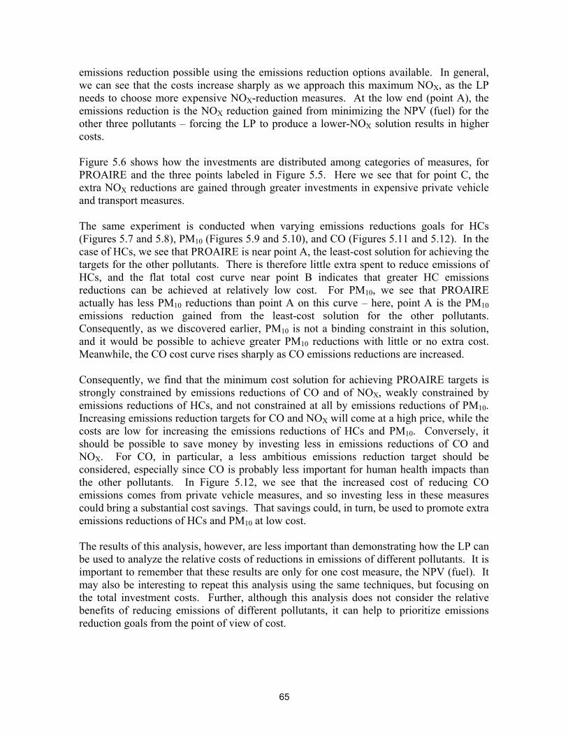
65

emissions reduction possible using the emissions reduction options available. In general, we can see that the costs increase sharply as we approach this maximum NOX, as the LP needs to choose more expensive NOX-reduction measures. At the low end (point A), the emissions reduction is the NOX reduction gained from minimizing the NPV (fuel) for the other three pollutants – forcing the LP to produce a lower-NOX solution results in higher costs. Figure 5.6 shows how the investments are distributed among categories of measures, for PROAIRE and the three points labeled in Figure 5.5. Here we see that for point C, the extra NOX reductions are gained through greater investments in expensive private vehicle and transport measures. The same experiment is conducted when varying emissions reductions goals for HCs (Figures 5.7 and 5.8), PM10 (Figures 5.9 and 5.10), and CO (Figures 5.11 and 5.12). In the case of HCs, we see that PROAIRE is near point A, the least-cost solution for achieving the targets for the other pollutants. There is therefore little extra spent to reduce emissions of HCs, and the flat total cost curve near point B indicates that greater HC emissions reductions can be achieved at relatively low cost. For PM10, we see that PROAIRE actually has less PM10 reductions than point A on this curve – here, point A is the PM10 emissions reduction gained from the least-cost solution for the other pollutants. Consequently, as we discovered earlier, PM10 is not a binding constraint in this solution, and it would be possible to achieve greater PM10 reductions with little or no extra cost. Meanwhile, the CO cost curve rises sharply as CO emissions reductions are increased. Consequently, we find that the minimum cost solution for achieving PROAIRE targets is strongly constrained by emissions reductions of CO and of NOX, weakly constrained by emissions reductions of HCs, and not constrained at all by emissions reductions of PM10. Increasing emissions reduction targets for CO and NOX will come at a high price, while the costs are low for increasing the emissions reductions of HCs and PM10. Conversely, it should be possible to save money by investing less in emissions reductions of CO and NOX. For CO, in particular, a less ambitious emissions reduction target should be considered, especially since CO is probably less important for human health impacts than the other pollutants. In Figure 5.12, we see that the increased cost of reducing CO emissions comes from private vehicle measures, and so investing less in these measures could bring a substantial cost savings. That savings could, in turn, be used to promote extra emissions reductions of HCs and PM10 at low cost. The results of this analysis, however, are less important than demonstrating how the LP can be used to analyze the relative costs of reductions in emissions of different pollutants. It is important to remember that these results are only for one cost measure, the NPV (fuel). It may also be interesting to repeat this analysis using the same techniques, but focusing on the total investment costs. Further, although this analysis does not consider the relative benefits of reducing emissions of different pollutants, it can help to prioritize emissions reduction goals from the point of view of cost.

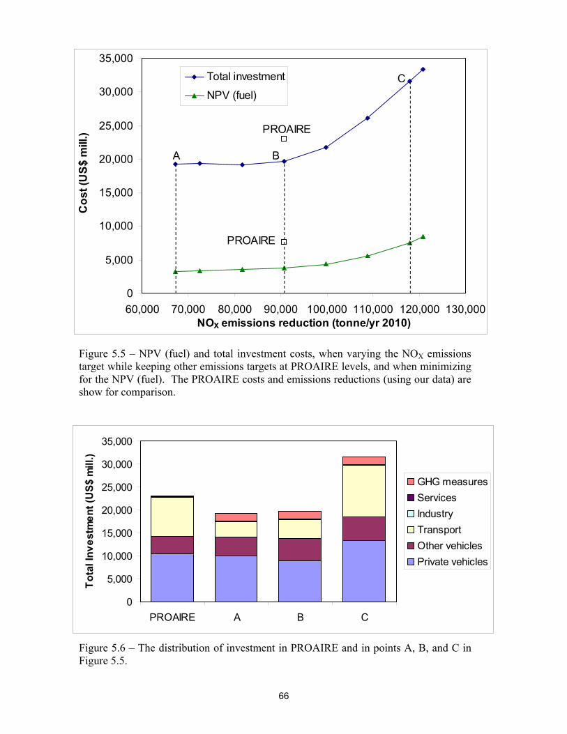
66

Figure 5.5 – NPV (fuel) and total investment costs, when varying the NOX emissions target while keeping other emissions targets at PROAIRE levels, and when minimizing for the NPV (fuel). The PROAIRE costs and emissions reductions (using our data) are show for comparison. Figure 5.6 – The distribution of investment in PROAIRE and in points A, B, and C in Figure 5.5.

0

5,000

10,000

15,000

20,000

25,000

30,000

35,000

60,000 70,000 80,000 90,000 100,000 110,000 120,000 130,000NOX emissions reduction (tonne/yr 2010)

Cos

t (U

S$ m

ill.)

Total investmentNPV (fuel)

PROAIRE

A

C

PROAIRE

B

0

5,000

10,000

15,000

20,000

25,000

30,000

35,000

PROAIRE A B C

Tota

l Inv

estm

ent (

US$

mill

.)

GHG measuresServicesIndustryTransportOther vehiclesPrivate vehicles

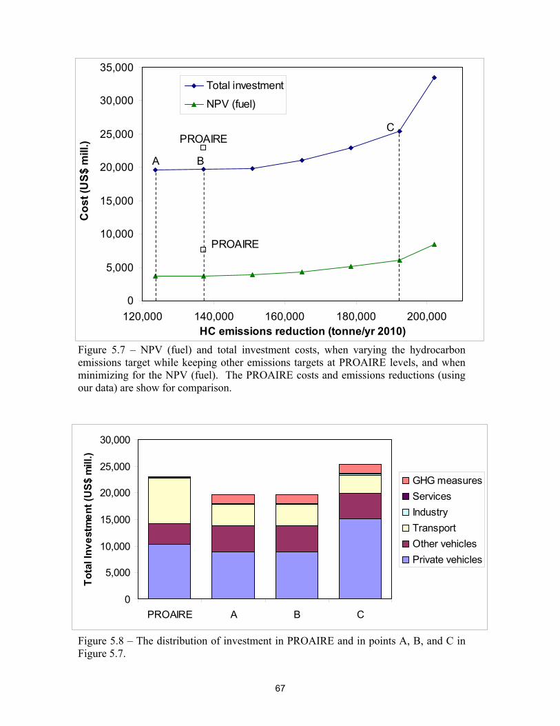
67

Figure 5.7 – NPV (fuel) and total investment costs, when varying the hydrocarbon emissions target while keeping other emissions targets at PROAIRE levels, and when minimizing for the NPV (fuel). The PROAIRE costs and emissions reductions (using our data) are show for comparison. Figure 5.8 – The distribution of investment in PROAIRE and in points A, B, and C in Figure 5.7.

0

5,000

10,000

15,000

20,000

25,000

30,000

PROAIRE A B C

Tota

l Inv

estm

ent (

US$

mill

.)

GHG measuresServicesIndustryTransportOther vehiclesPrivate vehicles

0

5,000

10,000

15,000

20,000

25,000

30,000

35,000

120,000 140,000 160,000 180,000 200,000HC emissions reduction (tonne/yr 2010)

Cos

t (U

S$ m

ill.)

Total investmentNPV (fuel)

PROAIRE

A

C

PROAIRE

B

68

Figure 5.9 – NPV (fuel) and total investment costs, when varying the PM10 emissions target while keeping other emissions targets at PROAIRE levels, and when minimizing for the NPV (fuel). The PROAIRE costs and emissions reductions (using our data) are show for comparison. Figure 5.10 – The distribution of investment in PROAIRE and in points A, B, and C in Figure 5.9.

0

5,000

10,000

15,000

20,000

25,000

30,000

35,000

3,500 4,000 4,500 5,000 5,500PM10 emissions reduction (tonne/yr 2010)

Cos

t (U

S$ m

ill.)

Total investmentNPV (fuel)

PROAIRE

A

C

PROAIRE

B

0

5,000

10,000

15,000

20,000

25,000

30,000

PROAIRE A B C

Tota

l Inv

estm

ent (

US$

mill

.)

GHG measuresServicesIndustryTransportOther vehiclesPrivate vehicles

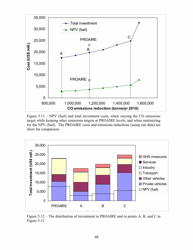
69

Figure 5.11 – NPV (fuel) and total investment costs, when varying the CO emissions target while keeping other emissions targets at PROAIRE levels, and when minimizing for the NPV (fuel). The PROAIRE costs and emissions reductions (using our data) are show for comparison. Figure 5.12 – The distribution of investment in PROAIRE and in points A, B, and C in Figure 5.11.

0

5,000

10,000

15,000

20,000

25,000

30,000

35,000

800,000 1,000,000 1,200,000 1,400,000 1,600,000CO emissions reduction (tonne/yr 2010)

Cos

t (U

S$ m

ill.)

Total investmentNPV (fuel)

PROAIRE

A

C

PROAIRE

B

0

5,000

10,000

15,000

20,000

25,000

30,000

PROAIRE A B C

Tota

l Inv

estm

ent (

US$

mill

.)

GHG measuresServicesIndustryTransportOther vehiclesPrivate vehiclesNPV (fuel)

70

5.2 Including emissions reduction targets for CO2 In the previous section, we focused only on meeting the local emission reduction targets. In this section, we consider adding targets for emissions reductions of CO2, in order to address the principal questions of this study, the co-control of urban air pollutants and GHGs. The approach taken here is to require the LP to meet emissions reduction targets for the four air pollutants (at PROAIRE emissions reduction levels) and then to vary the constraint on CO2 emissions. This is done first allowing only measures applied on the metropolitan scale (both PROAIRE measures and the GHG measures). Then we consider allowing emissions reduction actions for CO2 outside of the metropolitan area. 5.2.1 Using only measures applied locally In Figures 5.13 and 5.14, we vary the CO2 emissions target while meeting PROAIRE local emissions reductions targets, in experiments where we minimize the total investment cost, and minimize the NPV (fuel). The green curves show the results when minimizing the total investment, and the blue curves show the results when minimizing the NPV (fuel). These results are similar when minimizing for the two different cost measures. In both cases, the total investment cost is seen to increase as the CO2 emissions reduction increases, while the NPV (fuel) decreases. The costs rise substantially at high CO2 emissions reductions, as this approaches the limit of the CO2 emission reduction feasible using this database of measures. At low CO2 emissions reductions, below the minimum investment solution, the costs are also seen to rise. Here we are below the CO2 emissions reductions gained from the least-cost solution for the local pollutants, and CO2 is not a binding constraint. Here, the costs rise so sharply because we are forcing the LP to meet the emissions targets for local air pollutants in a less cost-efficient manner which has lower CO2 emissions. We consider feasible least-cost solutions in this range by forcing the constraint on the CO2 emissions reduction equal to some value, rather than using the “greater than or equal to” as we have in previous LP runs. For the case where the NPV (fuel) is minimized, the result of the LP is to invest as much as possible in the measures which have a negative NPV (fuel), even if these measures only have a small CO2 emissions reduction benefit. When minimizing the NPV (fuel), we use the same technique to obtain cost results at CO2 emissions reductions less than the minimum NPV (fuel) solution. The minimum NPV (fuel) and minimum total investment solutions are shown in Figures 5.13 and 5.14, when minimizing to achieve the local PROAIRE emissions reduction targets. These are the same solutions found in the previous section (see Figure 5.3). Here we see that these different solutions have very different CO2 emissions reductions associated with them, as mentioned before, but that they can be joined by a continuum of least-cost solutions in between them. Figure 5.15 shows the distribution of investments for the PROAIRE plan and for points A through F shown in Figures 5.13 and 5.14. Here we see that the results when minimizing the total investment or the NPV (fuel) do not differ greatly. In both cases, as the CO2 target is increased, the largest change in investment is in the GHG reduction measures.

71

Figure 5.13 – NPV (fuel) obtained when minimizing NPV (fuel) and total investment, while meeting the PROAIRE local emissions targets and varying the CO2 emissions target. Here we use only local measures, including the GHG measures. The right-most points approach the maximum CO2 emissions reduction possible using only the local measures. Figure 5.14 – As Figure 5.13, showing the total investment for the same conditions.

E

D

F Min. NPV

PROAIRE

AMin. Inv.

BC

0

1,000

2,000

3,000

4,000

5,000

6,000

7,000

8,000

9,000

0 2 4 6 8 10CO2 reduction (mill. tonnes CO2/yr 2010)

NPV

(fue

l) (U

S$ m

ill.)

Minimize Investment

Minimize NPV (fuel)

D

E

FMin. NPV

PROAIRE

AMin. Inv.

B

C

17,000

18,000

19,000

20,000

21,000

22,000

23,000

24,000

25,000

0 2 4 6 8 10CO2 reduction (mill. tonnes CO2/yr 2010)

Tota

l Inv

estm

ent (

US$

mill

.)

Minimize Investment

Minimize NPV (fuel)

72

Figure 5.15 – The distribution of investments in PROAIRE and in the least cost solutions while varying CO2 emissions reductions, shown in Figures 5.13 and 5.14. The changes in investment in the PROAIRE measures are small as CO2 emissions goals are varied, but these changes are not zero. Here, the LP had two general ways that the extra CO2 emissions reduction could be obtained: it could shift the investments in PROAIRE measures towards PROAIRE measures that reduce CO2 emissions, or it could invest in separate measures to obtain the GHG emissions reduction. In this case, the results of the LP indicate that it was more cost-effective to invest in GHG measures, rather than increasing investment in some of the PROAIRE measures. Investing in the GHG measures will cause some decrease in emissions of local air pollutants, and so therefore the burden of reducing local air pollutants can be reduced for the PROAIRE measures. Investing in GHG measures therefore reduces the investment required for PROAIRE measures. In Figure 5.15, however, this effect is observed to be small, as there is little change in PROAIRE investments. 5.2.2 Including CO2 reduction measures on a national scale In addition to actions applied on the metropolitan scale, policy-makers also have the ability to invest in CO2 emissions reductions outside of the metropolitan area, since the location of GHG emissions has very little effect on their climatic consequences. In this way, purchasing emissions on a national scale offers the potential for a large reservoir of possible CO2 emissions reductions, allowing the decision-maker to choose more CO2 reductions from the most cost-effective measures. Figures 5.16 to 5.18 show the same analysis as Figures 5.13 to 5.15, but allow the possibility of investing in CO2 emissions reductions on a national scale. As before, we show the cost results when minimizing for the two cost measures, and varying the CO2 emission reduction target while achieving the local PROAIRE emissions reduction targets. Here the results are somewhat different than the earlier results. When minimizing the total

0

5,000

10,000

15,000

20,000

25,000

PR

OA

IRE A B C D E F

Tota

l Inv

estm

ent (

US$

mill

.)

GHG measuresServicesIndustryTransportOther vehiclesPrivate vehiclesNPV (fuel)

73

investment, both cost measures show very little change as CO2 emissions reductions are increased. No dramatic increase in cost is seen at high CO2 emissions reductions since there is now the potential for very large CO2 emissions reductions, far beyond the range that we consider. In this case, the LP chooses the single measure that is most cost-effective for CO2 reductions in terms of the investment cost, which in this database of options is GN10, tropical forest management. Because there is a large potential for CO2 emissions reductions (sequestration) by using this measure in Mexico, this is the only measure chosen for additional CO2 emissions reduction. Since this measure has no effect on local air pollutant emissions, there is no change in the measures chosen to achieve the local air pollution emission reduction goals as the CO2 target is varied. Further, in Figure 5.16 it is clear that the investment costs for this measure are indeed very low, while the NPV (fuel) in the database of options is small and positive, causing the NPV (fuel) to increase slightly as CO2 emissions reductions targets are increased. This is also clear in Figure 5.18, which shows the distribution of investments in the different LP solutions. The results when minimizing the NPV (fuel) are different. In this case, if we only minimize the NPV (fuel) the result is a very large CO2 emissions reduction, taking advantage of all of the measures that have a negative NPV (fuel). While it is interesting to note that such a cost-saving strategy exists, it is probably not practical in the short term. We can explore other solutions by forcing the LP to consider lower CO2 reductions by setting the CO2 constraint as equal to the goal, rather than “less than or equal to.” The most cost-effective measures in terms of the NPV (fuel) for reducing CO2 emissions are several electricity efficiency measures, all of which have a negative NPV (fuel). Unlike the situation for tropical forest management, however, the maximum level of application of these measures nationally is small compared to the range of CO2 emissions reductions considered here. As the CO2 target is increased, therefore, the LP first reduces CO2 by investing in the most cost-effective (for NPV (fuel)) measure – first on the metropolitan scale and then nationally – and then investing in the next most cost-effective, and so on. Where the measures are applied on the metropolitan scale, the CO2 reduction comes with a benefit in terms reduced emissions of local air pollutants. This benefit reduces the burden on the PROAIRE measures for reducing local air pollutant emissions, and the investments in PROAIRE measures decrease slightly on account of this. Figure 5.18 shows both the increased investments in GHG measures, as the CO2 goal is increased, and the resulting decrease in the NPV (fuel).

74

Figure 5.16 – NPV (fuel) results when minimizing the total investment costs and NPV (fuel) for meeting the PROAIRE air pollutant emissions targets, while including different constraints on CO2 emissions. Here, national-scale CO2 emissions reductions measures are permitted, in addition to local measures. Figure 5.17 – Total investment costs for the same scenarios as shown in Figure 5.16.

F

D

EMin. NPV

local

PROAIRE

A Min. INV CB

0

1,000

2,000

3,000

4,000

5,000

6,000

7,000

8,000

0 2 4 6 8 10CO2 reduction (mill. tonnes CO2/yr 2010)

NPV

(fue

l) (U

S$ m

ill.)

Minimize Investment

Minimize NPV (fuel)

F

ED

Min. NPVlocal

PROAIRE

AMin. Inv. CB

17,000

18,000

19,000

20,000

21,000

22,000

23,000

0 2 4 6 8 10CO2 reduction (mill. tonnes CO2/yr 2010)

Tota

l Inv

estm

ent (

US$

mill

.)

Minimize Investment

Minimize NPV (fuel)

75

Figure 5.18 – The distribution of investments in PROAIRE and in the least cost solutions while varying CO2 emissions reductions, shown in Figures 5.16 and 5.17. As was the case when considering only actions on the metropolitan scale, we find that the CO2 emissions reductions are largely met by investments in GHG measures, rather than through an adjustment in the measures that address urban air pollutant emissions most cost-effectively. Where GHG measures are applied on the metropolitan scale, these measures have some benefit in terms of reducing local air pollutants and therefore reducing the burden on actions for controlling urban air pollutants. However, in both cases, this benefit is seen to be modest. Finally, the case where the total investment is minimized shows that under some circumstances, it may be most cost-effective to simply purchase CO2 emissions elsewhere, rather than modifying the urban air pollutant emissions plan to also reduce CO2. This suggests that even when considering metrics other than cost-effectiveness, policy-makers will be wise to also consider opportunities to reduce GHG emissions that are separate from their urban air pollution control measures, including outside of the metropolitan region. 5.3 Testing the testable hypothesis As stated in Chapter 1, we would like to test whether it is more cost-effective to plan to achieve local and global emissions reduction targets simultaneously, rather than planning them individually. The hypothesis that we consider is: Cost (Urban + Global) < Cost (Urban) + Cost (Global). To investigate this hypothesis, we consider the PROAIRE emissions reduction goals (for all pollutants except SO2) and a target reduction for CO2. We use the LP to minimize costs, allowing all of the measures applied at the metropolitan scale to be included in the database of options.

0

5,000

10,000

15,000

20,000

25,000

PR

OA

IRE A B C D E F

Tota

l Inv

estm

ent (

US$

mill

.)

GHG nationalGHG localServicesIndustryTransportOther vehiclesPrivate vehiclesNPV (fuel)

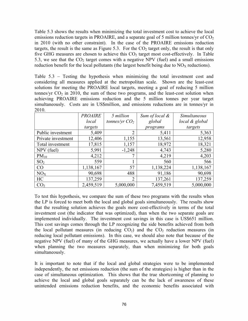
76

Table 5.3 shows the results when minimizing the total investment cost to achieve the local emissions reduction targets in PROAIRE, and a separate goal of 5 million tonnes/yr of CO2 in 2010 (with no other constraint). In the case of the PROAIRE emissions reduction targets, the result is the same as Figure 5.3. For the CO2 target only, the result is that only five GHG measures are chosen to achieve this CO2 target most cost-effectively. In Table 5.3, we see that the CO2 target comes with a negative NPV (fuel) and a small emissions reduction benefit for the local pollutants (the largest benefit being due to NOX reductions). Table 5.3 – Testing the hypothesis when minimizing the total investment cost and considering all measures applied at the metropolitan scale. Shown are the least-cost solutions for meeting the PROAIRE local targets, meeting a goal of reducing 5 million tonnes/yr CO2 in 2010, the sum of these two programs, and the least-cost solution when achieving PROAIRE emissions reduction and the 5 million tonnes per year target simultaneously. Costs are in US$million, and emissions reductions are in tonnes/yr in 2010.

PROAIRE local

targets

5 million tonnes/yr CO2

Sum of local & global

programs

Simultaneous local & global

targets Public investment 5,409 2 5,411 5,363 Private investment 12,406 1,155 13,561 12,958 Total investment 17,815 1,157 18,972 18,321 NPV (fuel) 5,991 -1,248 4,743 5,280 PM10 4,212 7 4,219 4,203 SO2 559 1 560 566 CO 1,138,167 57 1,138,224 1,138,167 NOX 90,698 488 91,186 90,698 HC 137,259 2 137,261 137,259 CO2 2,459,519 5,000,000 7,459,519 5,000,000

To test this hypothesis, we compare the sum of these two programs with the results when the LP is forced to meet both the local and global goals simultaneously. The results show that the resulting solution achieves the goals more cost-effectively in terms of the total investment cost (the indicator that was optimized), than when the two separate goals are implemented individually. The investment cost savings in this case is US$651 million. This cost savings comes through the LP recognizing the side benefits achieved from both the local pollutant measures (in reducing CO2) and the CO2 reduction measures (in reducing local pollutant emissions). In this case, we should also note that because of the negative NPV (fuel) of many of the GHG measures, we actually have a lower NPV (fuel) when planning the two measures separately, than when minimizing for both goals simultaneously. It is important to note that if the local and global strategies were to be implemented independently, the net emissions reduction (the sum of the strategies) is higher than in the case of simultaneous optimization. This shows that the true shortcoming of planning to achieve the local and global goals separately can be the lack of awareness of these unintended emissions reduction benefits, and the economic benefits associated with

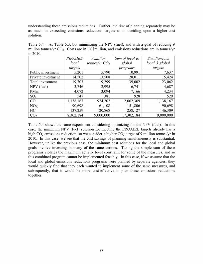
77

understanding these emissions reductions. Further, the risk of planning separately may be as much in exceeding emissions reductions targets as in deciding upon a higher-cost solution. Table 5.4 – As Table 5.3, but minimizing the NPV (fuel), and with a goal of reducing 9 million tonnes/yr CO2. Costs are in US$million, and emissions reductions are in tonnes/yr in 2010.

PROAIRE local

targets

9 million tonnes/yr CO2

Sum of local & global

programs

Simultaneous local & global

targets Public investment 5,201 5,790 10,991 7,637 Private investment 14,502 13,508 28,011 15,424 Total investment 19,703 19,299 39,002 23,062 NPV (fuel) 3,746 2,995 6,741 4,687 PM10 4,072 3,094 7,166 4,234 SO2 547 381 928 529 CO 1,138,167 924,202 2,062,369 1,138,167 NOX 90,698 61,108 151,806 90,698 HC 137,259 120,868 258,127 146,309 CO2 8,302,184 9,000,000 17,302,184 9,000,000

Table 5.4 shows the same experiment considering optimizing for the NPV (fuel). In this case, the minimum NPV (fuel) solution for meeting the PROAIRE targets already has a high CO2 emissions reduction, so we consider a higher CO2 target of 9 million tonnes/yr in 2010. In this case, we see that the cost savings of planning simultaneously is substantial. However, unlike the previous case, the minimum cost solutions for the local and global goals involve investing in many of the same actions. Taking the simple sum of these programs violates the maximum activity level constraint for some of the measures, and so this combined program cannot be implemented feasibly. In this case, if we assume that the local and global emissions reductions programs were planned by separate agencies, they would quickly find that they each wanted to implement some of the same measures, and subsequently, that it would be more cost-effective to plan these emissions reductions together.

78

Chapter 6

Development and Application of Goal Programming for Mexico City In addition to the application of a linear programming (LP) model for searching for minimum cost solutions, a goal programming (GP) method can also be useful for the CAM in exploring alternative sets of emissions control options. The advantage of the GP approach is that while the LP has one objective function to be optimized, the GP allows for multiple goals to be pursued simultaneously. The GP therefore does not optimize for one single goal. Rather it finds good solutions that reflect many priorities at the same time. This formulation of the problem is likely to be closer to how decision-makers envision a problem with multiple attributes about which they are concerned. In this chapter, the formulation of a GP is presented, as well as the application of the GP to emissions control in Mexico City. This application is intended to be illustrative of how a GP can be applied for such an emissions control problem. 6.1 Formulation of a GP model

Goal programming is based on linear programming, but allows for more than one objective to be considered, and expresses those as ‘goals’ rather than objectives. These goals are phrased as “we’d like to reduce emissions by at least XX tonnes/yr” and “we’d like to spend no more than $XX total.” The solution of the GP will satisfy all of these goals, if possible. Since it may not be possible to satisfy all goals simultaneously, the GP needs to be told which of the goals are more important than others. The different goals can be put in a strict hierarchy by setting different priorities to different goals (preemptive GP) – the GP ensures that the solution meets the Priority 1 goal, then the Priority 2 goal, if possible, and so on through all of the goals. There can also be many goals within a single priority class (1, 2, etc.), but these goals can be weighted differently to show the relative importance of meeting different goals (nonpreemptive GP). In our case, we have goals for cost (we have two cost indicators) and for emissions reductions of each of the pollutants we consider. We may also develop other quantitative indicators to reflect other policy goals. How we choose to express the priorities and weights of the goals should reflect the priorities of decision-makers as best we can. If there is a fixed budget to spend, we might set cost as the first priority and set the pollutant goals as second priority, weighted according to their relative importance in the atmosphere. The case where there are strict emissions reductions targets to be met at least cost, can be solved using the LP model presented earlier. Discussions with decision-makers and staff within CAM has suggested that there is no clear first-priority goal, and so setting all goals as equal priority but weighting those goals seems to be a sensible approach (nonpreemptive GP). The formulation of such a GP problem is:

79

Minimize: ∑=

−−++ +m

jjjjj wdwd

1)(

Subject to: ( )maxii AA ≤ for ni ...1=

0≥iA for ni ...1= Where:

for j = 1, j

n

iiij TCAd −= ∑

=

+

1)( , if j

n

iii TCA ≥∑

=1)(

∑=

− −=n

iiijj CATd

1

)( , if j

n

iii TCA <∑

=1

)(

0,0 =≥ −+jj ww

for j = 2…k+1, j

n

ijiij TEAd −= ∑

=

+

1, )( , if j

n

iii TEA ≥∑

=1

)(

∑=

− −=n

ijiijj EATd

1, )( , if j

n

iii TEA <∑

=1)(

0,0 ≥= −+jj ww

where +

jd and −jd are the positive and negative deviations from each goal j; +

jw and −jw are

the weights assigned to being over and under a goal; m is the number of goals; Ai is the activity level of pollution control measure i; (Ai)max is the maximum activity level allowable for measure i; n is the number of pollution control measures considered; Ci is the unit cost of implementing measure i; Tj is the goal (target) for indicator j; Ei,j is the unit emissions reduction of pollutant j due to implementation of pollution control measure i; and k is the number of pollutants considered. The GP is therefore actually an LP which is solved, but where the objective function is a weighted sum of the deviations from all of the goals (dj

+ and dj-), using the weights wj

+ and wj

-. These weights can be thought of as penalties or rewards, which can be defined differently for each goal. Where j = 1, this is the cost goal, which could use either of the two cost measures used in previous chapters. It is also possible to use both cost goals simultaneously, with a weighting between these goals. In this formulation of the GP, there will be penalty in the objective function if the cost exceeds the cost goal, but no benefit if the cost is less than the cost goal. This is called a “one-sided goal,” and is represented by the fact that wj

- = 0, while wj+ ≥ 0. The emissions reduction goals (for j = 2…k+1) are also

one-sided goals, but where the penalty is incurred if the emissions reduction is less than the goal. It is important to remember that the weights serve two purposes – they both convert units between the different goals and set weights for the goals relative to one another. A convenient way to handle this is to set the weighting for cost (w1

+) equal to 1.0 and express the weights for the different pollutants (wj

- for j = 2…k+1) relative to the cost. With this

80

formulation, the pollutant weights can be interpreted as the marginal willingness to pay for emissions reductions of each pollutant. This is a convenient formulation of the problem, which allows easy interpretation of the results, and will be used in this study. It also allows for the marginal willingness to pay to be informed by studies of the health effects of air pollution. We caution, however, that because of differences in units (costs over a time horizon and emissions reductions in the year 2010), this marginal willingness to pay cannot be compared with the results of other studies. This same caution was also raised in the previous chapter. A GP for this type of problem can also be expanded to include other types of goals, which may reflect the priorities of decision-makers, to the extent that indicators for these goals can be quantified. For this co-control problem addressing air pollution and climate change, other relevant indicators and goals include mobility and transportation, water quality and availability, technological and economic development, employment, and equity. We suggest that it can be beneficial to engage policy-makers in discussions of the importance of these goals, and to consider how these goals can be quantified meaningfully in an analysis of this type. 6.2 Application to Mexico City emissions control

For application of the GP to Mexico City, we use two different software frameworks. In MS Excel, the deviations from the goals can be calculated directly and from these, and the objective function can be calculated and minimized using the Solver function. In the DS2/QM software, a goal programming interface exists and can be used directly. In both software packages, however, we find that there are problems with solving a problem of the size represented by emissions control in Mexico City. In MS Excel, it is not possible to use the linear solver in the Solver function, and the nonlinear solver does not converge to the solution. In this case, it is necessary to change the initial conditions manually and run the solver repeatedly to try to converge to a better solution. This is more difficult when the problem size is large. In DS2/QM, the program does not succeed in running with a problem of this size. Further application of a GP for Mexico City should investigate different software frameworks. For these reasons, we use a limited set of possible options to reduce the size of the problem to one that DS2/QM can manage. Using this set, we can illustrate the use of the GP. We choose a set of 12 measures that represent the measures with the highest investment costs in the database of PROAIRE options, while also accounting for much of the emissions reduction potential. These options are V1&2, V6, V8, V9, V12&13, V21, V23, T25, T26, T27a, T27b, and T36, which are described in previous chapters. Using this set of measures, we first use the LP to find the minimum total investment cost solution for meeting emissions targets for PM10, CO, NOX and HCs, at a level equal to the sum of the emissions reductions of these 12 measures applied at the level in PROAIRE. This is the same as was done in the previous chapter, when optimizing to achieve PROAIRE emissions reductions. The solution of minimum total investment cost for this case is given in Table 6.1. This solution has PM10, CO, and NOX as binding constraints, with a small amount of excess HC emissions reduction above the constraint.

81

Table 6.1 – Minimum total investment cost (LP) solution, when using 12 possible PROAIRE measures, to meet emissions reductions targets of PM10 (2,772 tonnes/yr in 2010), CO (1,115,703), NOX (86,665) and HC (116,311). Costs are in US$million, emissions reductions are in tonnes per year in 2010, and shadow prices are US$million/(tonne/yr in 2010).

Measure Activity level Indicator Value V1&2 1.00 Total Investment 18,585 V6 1.00 NPV (fuel) 6,233 V8 1.10 PM10 2,772 V9 1.00 CO 1,115,703 V12&13 1.00 NOX 86,665 V21 1.01 HC 116,731 V23 0.99 CO2 1,991,845 T25 0.00 Shadow Prices T26 1.50 PM10 5.4094 T27a 1.50 CO 0.01608 T27b 0.37 NOX 0.003281 T36 0.00 HC 0.0

In the GP, this LP solution can be recreated by setting the cost (total investment) goal equal to the result of the LP, the weight for the cost (total investment) equal to 1.0, and the weights for each pollutant equal to the shadow prices found in running the LP. The result is the same as the LP result, with the value of the objective function in the GP equal to zero. This is an important check to ensure that the GP is formulated correctly. From this basis, the cost goal, pollutant reduction goals, and weights in the GP can be varied at will to reflect different priorities and to explore different good solutions. For illustration, we first consider the case where we want to achieve a greater reduction of PM10 emissions. For this case, we increase the goal for emissions reductions of PM10 by 10%. With this change in the PM10 goal, it is no longer possible to satisfy all goals simultaneously. If we keep the weight for PM10 at the value used earlier (the shadow price from the LP solution), or if we use a smaller value for the weight on PM10, then the same solution results as the LP run. The only difference is that now we are in violation of the goal for PM10 reduction, but because the weight is small, the GP chose to keep the same solution rather than find a new solution where the PM10 goal is satisfied but other goals (such as the cost) are not. If we then increase the weight on PM10, we can make PM10 reductions more important, and the GP will shift the solution to meet the PM10 goal while violating some of the other goals. In this case, we increase the weight on PM10 from 5.4094 US$million/(tonne/yr in 2010) to 10 US$million/(tonne/yr in 2010). The results are shown in Table 6.2. In this case, the total investment cost is observed to go up, as well as the emissions reductions of PM10. However, the emissions reductions of PM10 do not increase so much as to satisfy the PM10 goal – in this case, the GP chose to keep a balance by violating the goals for both total investment cost and PM10 emissions reductions. If we continue to increase the weight on

82

PM10, the GP would find a solution that satisfies the PM10 goal, while violating the cost goal more severely. We can also observe that the emissions reductions of the other pollutants also increased with respect to the previous solution, mainly as a co-benefit of the PM10 emissions reduction.

Table 6.2 – GP solution when using 12 possible PROAIRE measures, to meet the emissions reductions goals of Table 6.1, but with the goal for PM10 reductions increased by 10% (3049 tonne/yr in 2010). The weight on PM10 emissions reductions is set at 10 US$million/(tonne/yr in 2010). Costs are in US$million, and emissions reductions are in tonnes per year in 2010.

Measure Activity level Indicator Value V1&2 1.00 Total Investment 20,973 V6 1.00 NPV (fuel) 6,908 V8 1.10 PM10 2,998 V9 1.00 CO 1,180,257 V12&13 1.00 NOX 95,533 V21 0.99 HC 121,964 V23 1.80 CO2 2,389,865 T25 0.05 Weights T26 1.50 PM10 10.0 T27a 1.50 CO 0.01608 T27b 1.20 NOX 0.003281 T36 0.00 HC 0.0001

In addition to changing the emissions reductions goals and weights for different pollutants, we can also consider the two cost measures simultaneously. By also setting a goal for NPV (fuel), we can consider a tradeoff between the two cost measures, with the weight of NPV (fuel) indicating how important that is with respect to the total investment cost. In this formulation, the weight on the NPV (fuel) is dimensionless (US$million/US$million). With respect to the LP solution of Table 6.1, we keep the emissions reduction goals on the four pollutants the same, but decrease the goals for the total investment cost and the NPV (fuel) to 90% of the values in the LP solution. As with the case of raising the PM10 emissions reduction goal, reducing the cost goals (for both indicators) makes it impossible to achieve all goals simultaneously, and the GP must use the weights to weigh the different goals. If the weight on NPV (fuel) is small (0.1 or smaller), the resulting solution is the same as the LP solution (with some small numerical differences), with the solution in violation of both cost goals by 10%. If the weight on NPV (fuel) is increased, then meeting the NPV (fuel) goal becomes more of a priority. When the weight is in the range of 0.2 to 1.0, the balance between meeting the cost goals and the emissions reduction goals shifts towards meeting the cost goals, while violating the emissions reduction goals. The new result is shown in Table 6.3. The result violates the goals for the emissions reduction of each of the four pollutants. Interestingly, the goal for the total investment cost is exceeded (a lower cost than the goal), while the goal for NPV (fuel) is violated, even though we raised the weight on NPV (fuel). This suggests that for this set of measures, the two cost measures are closely related. We might expect a greater tradeoff between these cost

83

measures when the GHG mitigation measures are included in the option set, as we saw in the previous chapter.

Table 6.3 – GP solution when using 12 possible PROAIRE measures, to meet the emissions reductions goals of Table 6.1, but with the goals for the total investment cost and the NPV (fuel) decreased by 10%. The weight on NPV (fuel) is set at 0.2. Costs are in US$million, and emissions reductions are in tonnes per year in 2010.

Measure Activity level Indicator Value V1&2 1.00 Total Investment 16,687 V6 1.00 NPV (fuel) 5,847 V8 1.10 PM10 2,289 V9 1.00 CO 1,114,389 V12&13 1.00 NOX 73,882 V21 1.18 HC 116,518 V23 0.00 CO2 1,681,837 T25 0.00 T26 0.09 T27a 1.50 T27b 0.00 T36 0.00

As a final illustration of the model, the various targets and weights can be changed to explore different solutions, in an iterative process of deciding what weights reflect priorities, and of seeing the effects of those different representations on the preferred solution. By studying which measures are repeatedly included in or excluded from preferred solutions, the GP can help to prioritize the implementation of these emission reduction actions. This is illustrated by showing one such possible solution. Here we consider higher weights on PM10, NOX and HCs, with a smaller weight on CO, reflecting the likely relative importance of these pollutants for health. The emissions reductions goals for PM10, NOX and HCs are increased by 20% relative to the LP solution, while the two cost goals are decreased by 10%. The CO goal is kept the same as the LP solution. These goals and weights are shown in Table 6.4.

84

Table 6.4 – GP formulation and solution for illustrating different combinations of goals and weights. The LP solution for minimum total investment cost (from Table 6.1) is shown for comparison. Costs are listed in US$million, emissions reductions are in tonnes per year in 2010, and weights are US$million/(tonne/yr in 2010).

Indicator Goal Weight

GP Solution LP Solution

Total Investment 16,736 1.0 20,675 18,585 NPV (fuel) 5,601 0.33 6,629 6,233 PM10 3,326 9.0 3,192 2,772 CO 1,115,703 0.005 1,032,456 1,115,703 NOX 103,998 0.02 95,442 86,665 HC 140,077 0.03 109,028 116,731 CO2 2,399,562 1,991,845

The resulting solution in Table 6.4 is interesting because it violates all of the six goals, yet it could be considered a reasonably good solution on which to base an emissions control program. The costs are observed to increase relative to the LP solution, showing that the balance between emissions reduction and cost is shifted here slightly towards emissions reductions in this example. The measures that make up this solution are shown in Table 6.5. It is interesting to note, for example, that while the option to expand the Metro system (T25) was not included in the previous solutions to a significant extent, it is included in this solution where different goals are balanced.

Table 6.5 – The activity levels of measures in the GP solution shown in Table 6.4.

Measure Activity level V1&2 1.00 V6 1.00 V8 1.10 V9 1.00 V12&13 1.00 V21 0.73 V23 1.80 T25 0.60 T26 1.50 T27a 1.50 T27b 1.20 T36 0.00

6.3 Conclusions In summary, goal programming has been shown to be a potentially useful tool in exploring good emissions control plans where multiple pollutants (local and global) are considered. In contrast to the LP, the GP does not optimize for a single objective. Rather the GP allows the exploration of good solutions that balance competing priorities. In conversations with Mexican decision-makers and staff, this framework reflects more accurately how decision-

85

makers conceive of the emissions control problem. The GP has also been created in a framework that can be straightforward to understand and apply. In using the GP, studies of the health effects of different pollutants can be used to help set the weights. It is not, however, necessary to do this as the weights and goals can be changed somewhat arbitrarily to see what effects they have on the solution. The GP is best used in this iterative manner to explore different solutions, and to understand how they differ and what they have in common. In addition, it can be useful to use the GP and LP together in exploring different solutions, as illustrated in this chapter. For further application to the case of Mexico City emissions controls, it will be important to use a new software environment that will allow an easy and user-friendly solution to the GP, when all emissions reduction measures are included. These software frameworks will continue to be explored.

86

Chapter 7

Conclusions and Recommendations 7.1 Summary of completed work, and key findings We created a coherent, harmonized database of emissions reductions options for the MCMA, combining data from existing and disparate reports focused separately towards air quality management and mitigation of GHGs. In doing so, we combined existing information in such a way that the costs and emissions reductions are directly comparable between different measures. This database was constructed through an open process in which all offices within CAM participated, and all of our calculations and assumptions are fully documented in the calculation notes included as Appendices A and B of this report. 1) We corrected a number of apparent errors in PROAIRE, and changed cost and emissions reductions estimates using our own assumptions where appropriate. The net result was a significant increase in the total program costs of PROAIRE, and a significant increase in CO emissions reductions. Emissions reductions for other pollutants also changed significantly. 2) In creating this database of options, we estimated the GHG emissions implications of the new air quality program for PROAIRE, which was not previously known. Overall, we estimate that PROAIRE has a significant net benefit for reducing emissions of GHGs in Mexico City. We estimate that if the 22 PROAIRE measures that we considered are implemented as planned, a reduction in CO2 emissions will result of about 2.2 million tonnes CO2 per year in 2010. This is a reduction of about 3.1% from the baseline projected CO2 emissions for the MCMA in 2010. This reduction results about half from measures that improve vehicle technology and replace old vehicles with newer vehicles, and about half from investments to improve the transportation infrastructure. Five PROAIRE measures were estimated to cause a net increase in CO2 emissions. We should caution that for several of the measures, our estimates are still preliminary, while others could be improved with better data, such as actual data on the fuel efficiency of in-use vehicles in Mexico City. This reduction in CO2 emissions can be considered an important “co-benefit” of actions to improve urban air quality. 3) We also estimated the local air quality impact of the “GHG mitigation measures”, applied in the MCMA. These measures were not included in PROAIRE, and are motivated mainly towards GHG mitigation in the studies we reviewed. We find that if implemented to their full potential in the MCMA, the CO2 emissions reduction expected is about 8.7% of the total MCMA emissions in 2010. Meanwhile, the local air quality impact of these measures is much smaller than the reductions due to PROAIRE measures – reductions relative to 2010 projected emissions are 3.2% for HCs, 1.4% for NOX, and 1.3% for PM10. In part, the effect on local emissions is not larger because only a small fraction of the electricity consumed in the MCMA is generated locally. It should be noted, however, that decreasing electricity generation from local plants, together with implementing electricity efficiency measures, is an available policy option that can increase the benefits of these

87

measures. Further, implementing electricity efficiency measures will improve air quality elsewhere in Mexico, potentially also improving air quality in the MCMA, although this transport of air pollutants is not currently well quantified. 4) The GHG mitigation measures are often characterized by relatively large up-front investments, but show good returns or negative NPVs over a longer term, due to the significant savings in fuel or electricity consumption. This contrasts with the PROAIRE measures, where changes in expenditures on fuels or electricity are generally a smaller component of the NPV. 7.2 Recommendations concerning data quality and availability 1) Despite our significant efforts to ensure data quality, the costs and emissions reductions estimated in this study should be taken with some caution. The data are probably not of sufficient quality to draw definitive conclusions about the relative cost-effectiveness of individual measures, and more quantitative work and certainly more discussion of the qualitative benefits, costs and barriers of each measure should be considered in deciding between individual policies. These data are, however, of sufficient quality to demonstrate the use of the LP and GP in informing policy decisions. It is further of sufficient quality to learn lessons on a broader scale about the co-control of urban air pollutants and GHGs. 2) Our work to create a harmonized database of measures was significantly more difficult, and was limited in its quality, due to the severe lack of documentation in nearly all of the documents that we used in this study. Some basic questions of how estimates were made in the previous studies remain unanswered, while many of our calculations were made using our inferences, based on the best information available. No calculation notes exist for the PROAIRE document – although we did receive the spreadsheets used for calculations of emissions reductions, we still do not understand many of the cost calculations. Meanwhile, the documentation in the GHG mitigation studies was insufficient to recalculate the emissions reductions for all of the measures included. The exceptions to this were the separate studies of individual technologies for solar water heaters (Quintanilla et al., 2000), and for hybrid buses (Consultants to the World Bank, 2000). 3) PROAIRE, as well as the GHG mitigation studies and other past work in Mexico, puts much more emphasis on the emissions reductions estimates than on the cost estimates. The undiscounted investment costs in PROAIRE, while easy to understand and relevant for policy decisions, are a poor measure of the true economic impact of emissions control measures. The studies of solar water heaters (Quintanilla et al., 2000) and hybrid buses (Consultants to the World Bank, 2000), as well as the recent study by the World Bank (Cesar et al., 2002) and several detailed studies by the US EPA (1999; 2002), should serve as models for how the economic impact should be estimated, and for how to better document costs. 4) Future work using the cost data presented in this study should try to improve these estimates by considering a longer time horizon for the NPV calculations, and by including other changes in operation and maintenance costs besides those reflected in this study.

88

Other emissions reduction measures not considered in this study should likewise be quantified and included. 7.3 Results of quantitative policy analysis We used the harmonized database of measures as input to LP and GP methods for quantitative policy analysis. Our purposes in doing so are:

1) To develop and demonstrate such methods for use in decision-making among the member organizations of CAM.

2) To consider the relationship between controls on emissions of urban air pollutants and GHGs, in terms of devising cost-effective strategies for simultaneously addressing the two problems.

The main findings when applying the LP to the local goals of air quality improvement in Mexico City were: 1) The total cost of achieving air quality improvements can be reduced by increasing the emphasis on more cost-effective measures, while decreasing the emphasis on less cost-effective measures. When only PROAIRE measures are considered, we estimate that the maximum reductions in both the total investment costs and the NPV (fuel) is about 20%. While this least-cost solution is not necessarily the best policy, it is interesting to consider what emissions control measures are included in this solution, as they are likely the most cost-effective measures when controlling for multiple pollutants simultaneously. 2) Lower cost solutions were not possible mainly because PROAIRE measures are generally applied near the maximum level possible. The problem is therefore highly constrained. We showed that the potential for cost reductions using the LP is greater when we used a goal of 75% of the PROAIRE emissions reductions targets, as there is then greater potential to increase the investment in the most cost-effective actions. 3) When we include other measures from the GHG mitigation studies, the minimum total investment solution shows little change, but a significantly lower NPV (fuel) can be reached by investing significantly in GHG control measures as part of PROAIRE, with a significant benefit in terms of reduced CO2 emissions. These preferred measures include a number of electricity efficiency measures, industrial cogeneration of heat and electricity, and solar water heating. The implication is that while the local air quality effect of implementing these measures may not be large in comparison with PROAIRE measures, several of these measures are known to come at a net cost savings, and should be considered as potentially important measures in the local air quality plan. 4) By exploring the least-cost NPV (fuel) solution as a function of the level of control of individual pollutants, we found that the PM10 and HC emissions reductions goals in PROAIRE could be increased with relatively little change in costs (both NPV (fuel) and the total investment costs). Meanwhile, increasing the CO emissions target involves a large increase in costs, and there is a potential to save significantly by reducing the CO target and investing less in expensive measures involving private automobiles. This illustrates how

89

the LP can be used to help set the emissions reduction goals from the point of view of costs. The main conclusions from applying the LP to consider controls on GHG emissions, in addition to the PROAIRE targets for emissions of local pollutants, are: 1) When considering only actions implemented on a local scale, additional CO2 emissions reductions can be met most cost-effectively by investing in the GHG mitigation measures. Other possibilities of adjusting the investments in PROAIRE measures to achieve CO2 mitigation were found to be less cost-effective. Meanwhile, increasing the CO2 target is observed to cause an increase in total investment cost, but a significant decrease in the NPV (fuel), as measures with a negative NPV (fuel) are generally selected as most cost-effective. These results are consistent whether we minimize for the total investment cost or for NPV (fuel). The GHG mitigation measures do provide some benefits in reduced emissions of local pollutants, which relieves the need to invest in PROAIRE measures. However, we estimate that this savings in PROAIRE measures is small. 2) When we allow for CO2 emissions reductions to be purchased outside of the MCMA, the results differ strongly when we minimize for the total investment cost or for NPV (fuel). When minimizing the total investment cost, the option which provides CO2 mitigation at the least investment cost is tropical forest management. Since this measure has a very large potential for CO2 emissions reductions, a large reduction of CO2 emissions can be purchased at a low investment cost, but with an increase in NPV (fuel). In contrast, when minimizing the NPV (fuel), it is most cost effective to invest in several GHG measures which have negative NPV (fuel), applied both on a local scale (with some local air pollution benefit) and on a national scale. In both cases, it is estimated to be most cost-effective to have little change in the investment in PROAIRE measures, and invest mostly separately in the other GHG measures. 3) The result that it is most cost-effective to invest in GHG mitigation measures to achieve extra CO2 reductions, apart from the PROAIRE measures, results from the costs and emissions reductions in our database of options. We find that the most cost-effective means of reducing emissions of local air pollutants are not necessarily the most cost-effective for CO2. Meanwhile, the most cost-effective means of reducing CO2 have a small potential to decrease emissions of local air pollutants, especially when we consider the possibility of reducing CO2 emissions outside of the metropolitan area. We caution, however, that while this conclusion is illustrative of possible outcomes of this type of analysis, we cannot necessarily generalize this conclusion – we are using a limited list of measures, and a limited geographical scale (the MCMA) in which the air quality benefits of reduced electricity generation are small. This conclusion may not hold, for example, if we considered a larger geographical area, or if we applied these methods in other urban areas where a greater fraction of electricity may be generated locally. 4) The LP was used to demonstrate that planning to achieve mitigation goals for urban air pollutants and GHGs simultaneously is more cost-effective than planning separately, due to the “secondary” benefits of each type of measure. For policy, therefore, the main risk in planning separately may be in not recognizing these emissions reduction benefits.

90

5) In addition to the LP, goal programming was seen as a potentially very useful tool in considering multiple pollutant control. Here, the strength of GP is in balancing multiple different targets for cost and emissions reductions, rather than optimizing for a single indicator. 7.4 Recommendations concerning air quality and GHG management 1) Current plans for urban air quality improvements in Mexico City (PROAIRE) are seen to come with a significant “co-benefit” in terms of reduced emissions of GHGs. But these GHG emissions reductions do not come uniformly from all measures. As PROAIRE is re-evaluated, decision-makers might consider the GHG emissions implications of the different measures, as well as the results of the LP and GP models when constraints are placed on CO2 emissions, as factors which may influence the emphasis put on different PROAIRE measures. 2) While the effect of the GHG mitigation measures on local air quality is generally modest, these can be considered as part of a local air quality control plan, because several of these measures are estimated to come at a cost-savings over a longer term. For the measures which reduce electricity consumption, the benefit of reduced local air pollution is largely obtained outside of the MCMA – and the effects of such improvements on air quality in the MCMA are not well understood. Because of their up-front capital costs and because they often significantly reduce emissions of CO2, these measures can be seen as opportunities for foreign investment from international aid agencies and from other nations interested in purchasing GHG emissions reductions abroad. Among the more cost-effective of the GHG measures are solar water heating, and several measures that reduce electricity consumption: residential and commercial efficient lighting, efficient water pumping, and the industrial cogeneration of electricity. 3) The results of this study often indicate that the benefits of simultaneously planning urban air pollutant and GHG mitigation are small. For example, where a CO2 emissions reduction target was added to PROAIRE emissions reduction goals, the result was often to invest in CO2 control while making few changes in the PROAIRE measures. This conclusion in part reflects features that are particular to Mexico City, principally that the majority of electricity generation is remote from the metropolitan region. It will be interesting and important to repeat this study elsewhere to analyze how closely urban air pollutant and GHG mitigation are linked in other environments. 4) For the international co-benefits research community, this study has demonstrated that while some measures may have significant co-benefits for reducing emissions of both local and global pollutants, the best strategy to meet both local and global goals may come from a combination of separate local and global measures. Such possibilities were often not considered previously in co-benefits research, which tended to focus on “win-win” local-global measures. This study has shown that comprehensive “co-control” planning should begin by considering all possible measures, including those measures that may only reduce emissions of one pollutant (local or global).

91

5) When considering linking urban air quality management with control of GHG emissions, it is important to consider also opportunities outside of the metropolitan region. Since it does not matter (from a climatic perspective) where GHG emissions reductions occur, a best solution (in this study, a least-cost solution) may be to control urban air the best way possible, while investing in GHG control measures elsewhere. It is also important now to train those engaged in urban air quality management to consider also CO2 control simultaneously – in order to plan better for GHG mitigation over a longer term. We suggest that it is important to engage air quality planners in analysis involving co-control on the urban scale, as illustrated in this study, even if the result of such planning may be to invest in actions to reduce CO2 outside of the metropolitan region.

92

References Burtraw, D., and M. Toman (1997) The benefits of reduced air pollutants in the US from

greenhouse gas mitigation policies, Resources for the Future, Discussion paper 98-01-REV, www.rff.org.

CAM (Comisión Ambiental Metropolitana) (2001) Inventario de emisiones a la atmósfera,

Zona Metropolitana del Valle México, 1998. Mexico City. CAM (Comisión Ambiental Metropolitana) (2002) Programa para mejorar la calidad del

aire de la Zona Metropolitana del Valle de México, 2002-2010. Mexico City. Cesar, H., G. Schadler, M. Hojer, P. Cicero-Fernández, L. Brandler, T. Buhl, A. Choperena

V., K. Doorland, A. González M., H. Hasselknippe, P. Montufar O., A. Velásquez M., A. Salcido, J. Sarmiento, and P. Van Beukering (2002) Air Pollution Abatement in México City: An Economic Evaluation, Report to the World Bank, draft of Feb. 5, 2002.

Cifuentes, L., V. H. Borja-Aburto, N. Gouveia, G. Thurston, and D. L. Davis (2001)

Hidden Health Benefits of Greenhouse Gas Mitigation, Science, 293:1257-1259. COMETRAVI (1999) Estrategia Integral de Transporte y Calidad del Aire para la Zona

Metropolitana del Valle de México, Study No. 8 Consultants to World Bank (2000) Estudio de prefactibilidad para la introducción de

autobuses híbridos en la prestación del servicio público de transporte de pasajeros en la ZMVM, June, 2000.

Ekins, P. (1996) The secondary benefits of CO2 abatement: How much emission reduction

do they justify? Ecological Economics, 19: 13-24. Eskeland, G. S., and J. Xie (1998) Acting globally while thinking locally: Is the global

environment protected by transport emission control programs?, report from the World Bank, August, 1998.

IPCC (1996) Revised 1996 IPCC guidelines for national greenhouse gas inventories:

Reference manual, available at www.ipcc-nggip.iges.or.jp/public/gl/invs6a.htm. Masera, O., and C. Sheinbaum (draft) Mitigación de emisiones de carbono y prioridiades

de desarrollo nacional, Instituto de Ecología and Instituto de Ingeniería, UNAM, 50 p. Morales D., R. (2001) Identificación de barreras y oportunidades para reducir emisiones

de gases efecto invernadero y de contaminantes locales con prioridad en las emisiones de NOX en termoeléctricas de la Zona Metropolitana de la Ciudad de México, September, 2001.

93

NREL (National Renewable Energy Laboratory) (2000) Developing Country Case-Studies: Integrated Strategies for Air Pollution and Greenhouse Gas Mitigation, Progress report for the International Co-control Benefits Analysis Program, November, 2000.

Northeast Advanced Vehicle Consortium, M. J. Bradley & Associates, and West Virginia

University (2000) Hybrid-electric drive heavy-duty vehicle testing project, final emissions report, available at www.mjbradley.com/documents/Navc9837.pdf.

Quintanilla M., J., M. Bauer E., J. A. Valdez P., E. J. Preciat L., F. Paz G., G. Ortega R., N.

Sánchez H., E. Morones E., O. Martínez A., A. García G., and A. Rojas M. (2000) Uso Masivo de la energía solar en sustitución de combustibles fósiles en la Zona Metropolitana del Valle de México: Sectores residencial, hospitalario, hotelero, y de baños públicos, Programa Universitario de Energía, UNAM, December, 2000.

SEMARNAT and INE (2001) Mexico: Second National Communication to the United

Nations Framework Convention on Climate Change, Mexico. Sheinbaum, C. (1997) Support for a climate change national plan for Mexico: Final report

to the USAID, Instituto de Ingeniería, UNAM, Agreement no. 523-0616-G-00-6058-00, December, 1997.

Sheinbaum, C., and O. Masera (2000) Mitigating carbon emissions while advancing

national development priorities: the case of Mexico, Climatic Change, 47: 259-282. Sheinbaum P., C., L. Ozawa, O. Vázquez, and G. Robles (2000) Inventario de emisiones de

gases de efecto invernadero asociados a la producción y uso de la energía en la Zona Metropolitana del Valle de México: Informe final, Grupo de Energía y Ambiente, Instituto de Ingeniería, UNAM, report to the Comisión Ambiental Metropolitana and the World Bank, September, 2000.

TUV Rheinland de Mexico, S. A. de C. V. (2000) Programa para la reducción y

eliminación de fugas de Gas LP, en las instalaciones domésticas de la Zona Metropolitana del Valle de México, August, 2000.

US EPA (1999) Regulatory impact analysis – control of emissions from new motor

vehicles, EPA-420-R-99-023. US EPA (2002) Draft technical support document: Nonconformance penalties for 2004

highway heavy duty diesel engines, EPA420-D-02-001, January, 2002. WGPHFC (Working Group on Public Health and Fossil-Fuel Combustion) (1997) Short-

term improvements in public health from global-climate policies on fossil fuel combustion: an interim report, Lancet, 350: 1341-1349.