University of Tennessee, KnoxvilleTrace: Tennessee Research and CreativeExchange

Masters Theses Graduate School

12-2003

Itera- tive Reconstruction Framework for High-Resolution X-ray CT DataThomas Matthew BensonUniversity of Tennessee - Knoxville

This Thesis is brought to you for free and open access by the Graduate School at Trace: Tennessee Research and Creative Exchange. It has beenaccepted for inclusion in Masters Theses by an authorized administrator of Trace: Tennessee Research and Creative Exchange. For more information,please contact trace@utk.edu.

Recommended CitationBenson, Thomas Matthew, "Itera- tive Reconstruction Framework for High-Resolution X-ray CT Data. " Master's Thesis, University ofTennessee, 2003.https://trace.tennessee.edu/utk_gradthes/1900

To the Graduate Council:

I am submitting herewith a thesis written by Thomas Matthew Benson entitled "Itera- tiveReconstruction Framework for High-Resolution X-ray CT Data." I have examined the final electroniccopy of this thesis for form and content and recommend that it be accepted in partial fulfillment of therequirements for the degree of Master of Science, with a major in Computer Science.

Jens Gregor, Major Professor

We have read this thesis and recommend its acceptance:

Jian Huang, Michael Thomason

Accepted for the Council:Carolyn R. Hodges

Vice Provost and Dean of the Graduate School

(Original signatures are on file with official student records.)

To the Graduate Council:

I am submitting herewith a thesis written by Thomas Matthew Benson entitled “Itera-

tive Reconstruction Framework for High-Resolution X-ray CT Data.” I have examined

the final electronic copy of this thesis for form and content and recommend that it be

accepted in partial fulfillment of the requirements for the degree of Master of Science,

with a major in Computer Science.

Jens Gregor

Dr. Jens Gregor, Major Professor

We have read this thesisand recommend its acceptance:

Jian Huang

Michael Thomason

Accepted for the Council:

Anne Mayhew

Vice Provost and Dean of Graduate Studies

(Original signatures are on file with official student records.)

Iterative Reconstruction Framework for

High-Resolution X-ray CT Data

A Thesis

Presented for the

Master of Science

Degree

The University of Tennessee, Knoxville

Thomas M. Benson

December, 2003

Acknowledgments

I would like to thank Dr. Jens Gregor for devoting a great deal of time to advising

me during this work. His assistance has been crucial during the course of this thesis and

is much appreciated. I would also like to thank my family for their continued support

during my prolonged affiliation with the educational system.

This work was supported by the National Institutes of Health under grant number

1 R01 EB00789-01A2. The computer equipment was acquired as part of SInRG, a

University of Tennessee grid infrastructure grant supported by the National Science

Foundation under grant number EIA-9972889.

ii

Abstract

Small animal medical imaging has become an important tool for researchers as it

allows noninvasively screening animal models for pathologies as well as monitoring dis-

ease progression and therapy response. Currently, clinical CT scanners typically use a

Filtered Backprojection (FBP) based method for image reconstruction. This algorithm

is fast and generally produces acceptable results, but has several drawbacks. Firstly,

it is based upon line integrals, which do not accurately describe the process of X-ray

attenuation. Secondly, noise in the projection data is not properly modeled with FBP.

On the other hand, iterative algorithms allow the integration of more complicated sys-

tem models as well as robust scatter and noise correction techniques. Unfortunately,

the iterative algorithms also have much greater computational demands than their FBP

counterparts. In this thesis, we develop a framework to support iterative reconstruc-

tions of high-resolution X-ray CT data. This includes exploring various system models

and algorithms as well as developing techniques to manage the significant computa-

tional and system storage requirements of the iterative algorithms. Issues related to the

development of this framework as well as preliminary results are presented.

iii

Contents

1 Introduction 1

2 Image Reconstruction as a Linear System 7

2.1 Mathematical Foundations . . . . . . . . . . . . . . . . . . . . . . . . . . 7

2.1.1 Projections . . . . . . . . . . . . . . . . . . . . . . . . . . . . . . 8

2.1.2 X-Ray Attenuation . . . . . . . . . . . . . . . . . . . . . . . . . . 10

2.2 Representation as a Linear System . . . . . . . . . . . . . . . . . . . . . 14

2.3 Modeling Techniques . . . . . . . . . . . . . . . . . . . . . . . . . . . . . 15

2.3.1 Ideal Model . . . . . . . . . . . . . . . . . . . . . . . . . . . . . . 16

2.3.2 Single Line Intersection Model . . . . . . . . . . . . . . . . . . . 16

2.3.3 Multiple Line Based Model . . . . . . . . . . . . . . . . . . . . . 19

2.3.4 Trilinear Interpolation Model . . . . . . . . . . . . . . . . . . . . 20

3 Survey of Algorithms 24

3.1 Algebraic Reconstruction Techniques . . . . . . . . . . . . . . . . . . . . 24

3.1.1 Algebraic Reconstruction Preliminaries . . . . . . . . . . . . . . 25

iv

3.1.2 SART . . . . . . . . . . . . . . . . . . . . . . . . . . . . . . . . . 26

3.2 Statistical Reconstruction Techniques . . . . . . . . . . . . . . . . . . . 28

3.2.1 Expectation Maximization . . . . . . . . . . . . . . . . . . . . . . 28

3.2.2 Weighted Least Squares . . . . . . . . . . . . . . . . . . . . . . . 32

4 Managing the System Matrix 37

4.1 Explicit Storage . . . . . . . . . . . . . . . . . . . . . . . . . . . . . . . . 38

4.2 Sparse Storage . . . . . . . . . . . . . . . . . . . . . . . . . . . . . . . . 38

4.3 System Symmetries . . . . . . . . . . . . . . . . . . . . . . . . . . . . . . 40

4.3.1 Overview of Symmetries . . . . . . . . . . . . . . . . . . . . . . . 40

4.3.2 Mathematical Formulation of Symmetries . . . . . . . . . . . . . 41

4.3.3 Limitations of Symmetries . . . . . . . . . . . . . . . . . . . . . . 44

4.3.4 Implementation of Symmetries . . . . . . . . . . . . . . . . . . . 45

4.4 Disk storage . . . . . . . . . . . . . . . . . . . . . . . . . . . . . . . . . . 47

4.5 Implementation Issues . . . . . . . . . . . . . . . . . . . . . . . . . . . . 48

4.5.1 Spherical Support Region . . . . . . . . . . . . . . . . . . . . . . 48

4.5.2 Multi-Threading . . . . . . . . . . . . . . . . . . . . . . . . . . . 49

4.5.3 Load Distribution via MPI . . . . . . . . . . . . . . . . . . . . . 49

5 Experimental Results 53

5.1 Computing Environment . . . . . . . . . . . . . . . . . . . . . . . . . . . 53

5.2 System Model Analysis . . . . . . . . . . . . . . . . . . . . . . . . . . . 54

5.2.1 Ideal Model . . . . . . . . . . . . . . . . . . . . . . . . . . . . . . 54

v

5.2.2 Single Line Intersection Model . . . . . . . . . . . . . . . . . . . 55

5.2.3 Multiple Line Intersection Model . . . . . . . . . . . . . . . . . . 59

5.2.4 Trilinear Interpolation Model . . . . . . . . . . . . . . . . . . . . 61

5.3 3D Shepp-Logan Phantom Reconstructions . . . . . . . . . . . . . . . . 63

5.4 Mouse Data Reconstructions . . . . . . . . . . . . . . . . . . . . . . . . 68

5.5 Storage Analysis . . . . . . . . . . . . . . . . . . . . . . . . . . . . . . . 71

5.6 Performance Analysis . . . . . . . . . . . . . . . . . . . . . . . . . . . . 73

5.6.1 System Model Analysis . . . . . . . . . . . . . . . . . . . . . . . 73

5.6.2 Iteration Analysis . . . . . . . . . . . . . . . . . . . . . . . . . . 75

5.6.3 Overall Performance . . . . . . . . . . . . . . . . . . . . . . . . . 76

6 Conclusions and Future Work 79

Bibliography 82

Vita 86

vi

List of Tables

4.1 Symmetries based on reflection . . . . . . . . . . . . . . . . . . . . . . . 43

4.2 Voxel index updates for symmetries . . . . . . . . . . . . . . . . . . . . . 47

5.1 System matrix storage requirements. . . . . . . . . . . . . . . . . . . . . 71

vii

List of Figures

1.1 MicroCAT geometry (courtesy of J. Cates) . . . . . . . . . . . . . . . . 2

2.1 Radon transform geometry . . . . . . . . . . . . . . . . . . . . . . . . . 9

2.2 Fanbeam sinogram of a mouse . . . . . . . . . . . . . . . . . . . . . . . . 11

2.3 Line intersections with pixels . . . . . . . . . . . . . . . . . . . . . . . . 18

4.1 Scanning circle octants. . . . . . . . . . . . . . . . . . . . . . . . . . . . 41

4.2 All symmetries of SD. . . . . . . . . . . . . . . . . . . . . . . . . . . . . 41

4.3 Projection ray SD (points). . . . . . . . . . . . . . . . . . . . . . . . . . 42

4.4 Reflection of SD (points). . . . . . . . . . . . . . . . . . . . . . . . . . . 42

4.5 Projection ray SD (angles). . . . . . . . . . . . . . . . . . . . . . . . . . 43

4.6 Reflection of SD (angles). . . . . . . . . . . . . . . . . . . . . . . . . . . 43

4.7 Partial forward projection. . . . . . . . . . . . . . . . . . . . . . . . . . . 51

4.8 Partial backprojection . . . . . . . . . . . . . . . . . . . . . . . . . . . . 51

5.1 Ideal voxel support for a given transaxial slice. . . . . . . . . . . . . . . 56

5.2 Central profile of ideal voxel support. . . . . . . . . . . . . . . . . . . . . 56

viii

5.3 Contour of slice 99. . . . . . . . . . . . . . . . . . . . . . . . . . . . . . . 58

5.4 Profile of slice 99. . . . . . . . . . . . . . . . . . . . . . . . . . . . . . . . 58

5.5 Artifacts resulting from single line based model. . . . . . . . . . . . . . . 59

5.6 Standard deviations for slice 99. . . . . . . . . . . . . . . . . . . . . . . . 61

5.7 Profiles of voxel support for transaxial slice 99. . . . . . . . . . . . . . . 62

5.8 Trilinear interpolation voxel support. . . . . . . . . . . . . . . . . . . . . 64

5.9 Original phantom. . . . . . . . . . . . . . . . . . . . . . . . . . . . . . . 65

5.10 Phantom reconstructions of transaxial slice 99. . . . . . . . . . . . . . . 65

5.11 Profiles of transaxial slice 99, coronal slice 114. . . . . . . . . . . . . . . 67

5.12 Mouse reconstuctions (transaxial slice 350). . . . . . . . . . . . . . . . . 69

5.13 Mouse reconstuctions (transaxial slice 450). . . . . . . . . . . . . . . . . 70

5.14 Distribution of system matrix across cluster nodes. . . . . . . . . . . . . 72

5.15 Line intersection based system model computation timings. . . . . . . . 74

5.16 Cost distribution per iteration (main memory). . . . . . . . . . . . . . . 76

5.17 Cost distribution per iteration (disk storage). . . . . . . . . . . . . . . . 77

ix

Chapter 1

Introduction

Small animal medical imaging has become an important tool for researchers as it al-

lows noninvasively screening animal models for pathologies as well as monitoring dis-

ease progression and therapy response. In support of the Mammalian Genetics Re-

search Facility at Oak Ridge National Laboratory, an X-ray micro-CT scanner, the

MicroCATTM

(ImTek, Inc., TN), has been developed for the imaging of laboratory mice

[4], [10]. This scanner has since been transferred to industry for commercialization.

The MicroCAT scanner acquires projection data of an object using a cone beam

geometry, which will be illustrated shortly. The MicroCAT acquires projections on a

CCD/phosphor screen detector. The CCD array is bonded to the phosphor screen,

which is sensitive to X-ray energies, using a 2:1 fiber optic taper. The X-ray source and

detector move in tandem in a circular orbit around the object. The geometry for the

MicroCAT is shown in figure 1.1.

1

source and

detector

trajectory

object

detector

array

source

fan of

fanbeams

midplane

axis of rotation

Figure 1.1. MicroCAT geometry (courtesy of J. Cates)

2

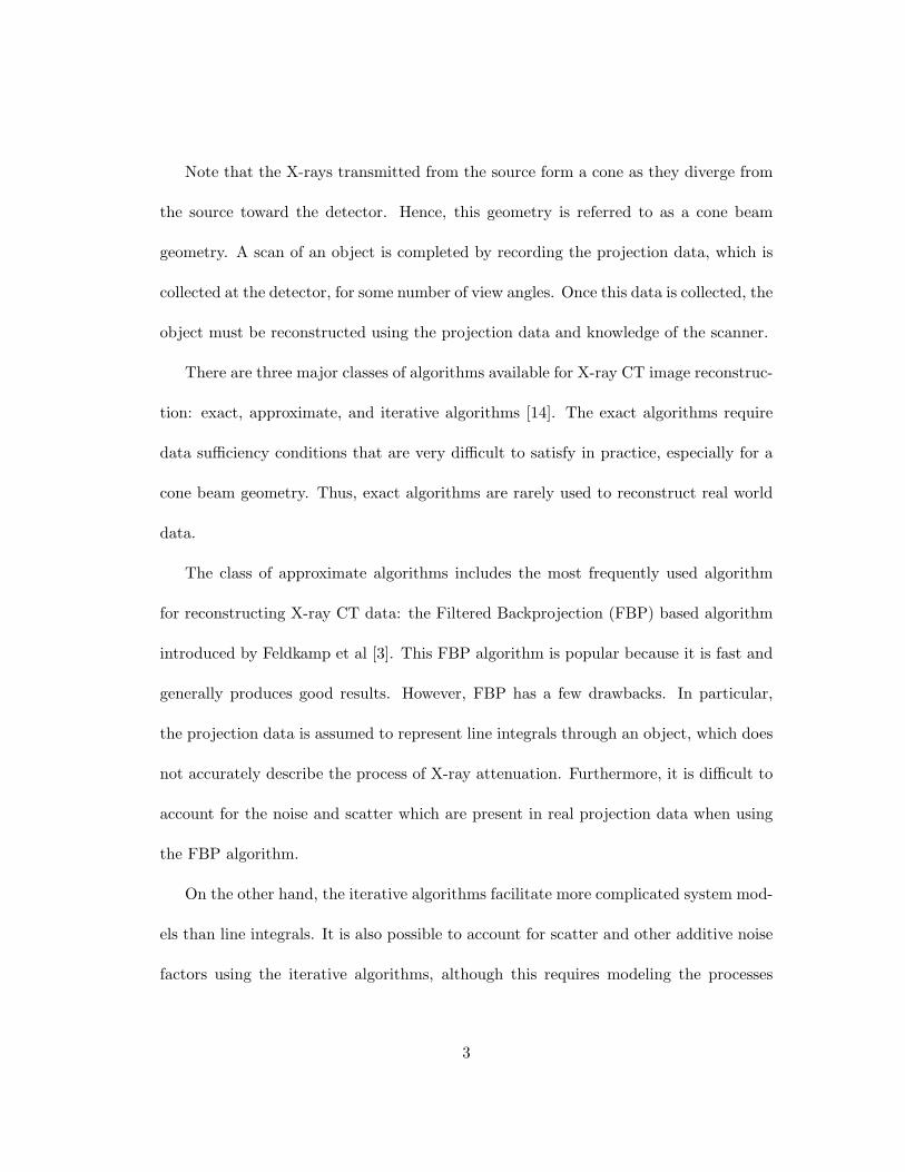
Note that the X-rays transmitted from the source form a cone as they diverge from

the source toward the detector. Hence, this geometry is referred to as a cone beam

geometry. A scan of an object is completed by recording the projection data, which is

collected at the detector, for some number of view angles. Once this data is collected, the

object must be reconstructed using the projection data and knowledge of the scanner.

There are three major classes of algorithms available for X-ray CT image reconstruc-

tion: exact, approximate, and iterative algorithms [14]. The exact algorithms require

data sufficiency conditions that are very difficult to satisfy in practice, especially for a

cone beam geometry. Thus, exact algorithms are rarely used to reconstruct real world

data.

The class of approximate algorithms includes the most frequently used algorithm

for reconstructing X-ray CT data: the Filtered Backprojection (FBP) based algorithm

introduced by Feldkamp et al [3]. This FBP algorithm is popular because it is fast and

generally produces good results. However, FBP has a few drawbacks. In particular,

the projection data is assumed to represent line integrals through an object, which does

not accurately describe the process of X-ray attenuation. Furthermore, it is difficult to

account for the noise and scatter which are present in real projection data when using

the FBP algorithm.

On the other hand, the iterative algorithms facilitate more complicated system mod-

els than line integrals. It is also possible to account for scatter and other additive noise

factors using the iterative algorithms, although this requires modeling the processes

3

involved. The major drawback to the iterative algorithms is the massively increased

storage and computational requirements. Due to these increased costs, iterative al-

gorithms are rarely used for three dimensional X-ray CT reconstructions. However,

iterative algorithms are heavily used for Positron Emission Tomography (PET) and

Single Photon Emission Computed Tomography (SPECT) due to the lower computa-

tional requirements and increased noise and scatter levels.

As computer technology advances, three dimensional iterative CT reconstructions

are becoming more feasible. The goal of this thesis is to develop a framework to support

high-resolution iterative reconstructions of X-ray CT data. This framework needs to

provide mechanisms to compute and store a very large system matrix and to perform

iterative solution techniques using this system matrix. Furthermore, the framework

should support easily replacing the system model used to compute the system matrix

and the iterative algorithm used to approximate a solution. Once developed, we can

utilize this framework to perform feasibility studies and comparative analysis on various

system models and iterative algorithms used for iterative X-ray CT reconstructions.

The decision to store the system matrix is rather unique. In general, due to the

massive space requirements involved in storing the system matrix, the matrix values are

recomputed as needed. However, since the entire matrix is needed for each iteration,

these values must be recomputed at least once per iteration. For most iterative algo-

rithms, the matrix values are actually needed twice per iteration. One of the design

goals of our iterative reconstruction framework is to avoid recomputing the system ma-

4

trix to increase performance. Note that there is also a body of literature exploring the

use of different system models based upon the operation being performed. These are

referred to as unmatched projectors [17] and are used to reduce the computation time

involved in generating the system matrix. However, since we store the system matrix,

we do not explore the use of unmatched projectors.

The first step of this thesis is to derive the reconstruction problem in terms of a

linear system and define each of the components of that linear system. This involves

describing the nature of the available data and some potential system models. The

system models include line intersection based models and a trilinear interpolation based

model. A fast algorithm for finding the intersections for the line intersection based

models was proposed by Siddon [13] and improved by Jacobs et al [5]. We address these

issues in chapter 2.

After stating the reconstruction problem in terms of a linear system, we must eval-

uate potential solutions of the linear system. These solutions take the form of iterative

algorithms and are introduced in chapter 3. The algorithms used in this thesis include

the Simultaneous Algebraic Reconstruction Technique (SART) proposed by Andersen

and Kak [6], the Expectation Maximization (EM) algorithm proposed independently

by Shepp and Vardi [12] and Lange and Carson [7], and a Weighted Least Squares

technique proposed by Fessler [2].

Due to the potentially massive size of the system matrix, we must address matrix

storage issues, which is the goal of chapter 4. Techniques used to manage the system ma-

5

trix include sparse matrix storage, the exploitation of symmetries, and load distribution

via the Message Passing Interface (MPI).

We present results of this work in chapter 5. These results include a preliminary

system model analysis as well as several iterative reconstructions. We also address the

system matrix storage and timing requirements for several reconstructions. Finally,

chapter 6 contains the conclusions as well as possible directions for future work.

6

Chapter 2

Image Reconstruction as a Linear

System

The first step in reconstructing images from a data set is to represent the reconstruction

problem in mathematical terms so that a solution can be deduced or approximated. For

many of the iterative reconstruction algorithms, including all algorithms considered

in this thesis, the basic mathematical model takes the form of a linear system. We

formulate the general structure of this linear system in the following sections.

2.1 Mathematical Foundations

The goal of X-ray computed tomography is to reconstruct some object based only on

projections of that object. Essentially, projection data records the effects of a given

object on an X-ray beam along a known path. Based on this data, we can reconstruct

7

an approximate attenuation map of the scanned object. For the purposes of this thesis,

an attenuation map is a collection of values that describes, in relative terms, the influence

of a spatial location on the attenuation of an X-ray beam. When discretized into a three

dimensional voxel space, the value of each voxel represents the average effect of that

voxel on the attenuation of the X-ray. We can then directly visualize the object by

interpreting the coefficients of the attenuation map as gray scale intensity values.

2.1.1 Projections

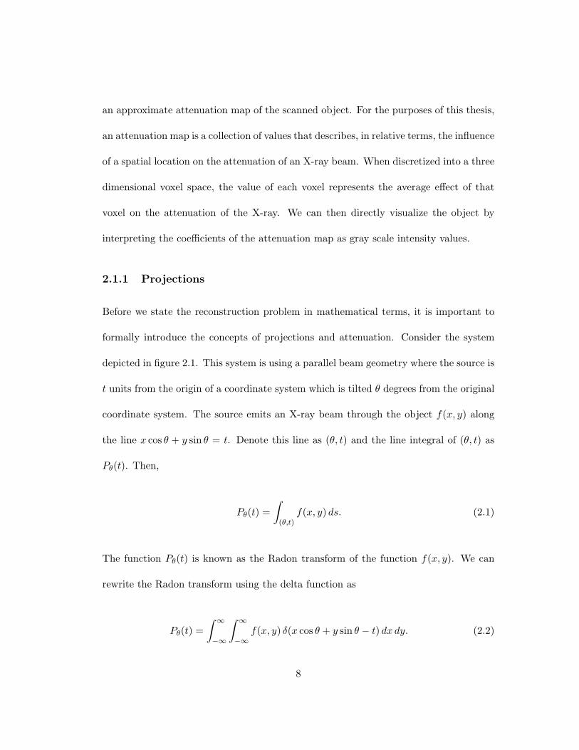
Before we state the reconstruction problem in mathematical terms, it is important to

formally introduce the concepts of projections and attenuation. Consider the system

depicted in figure 2.1. This system is using a parallel beam geometry where the source is

t units from the origin of a coordinate system which is tilted θ degrees from the original

coordinate system. The source emits an X-ray beam through the object f(x, y) along

the line x cos θ + y sin θ = t. Denote this line as (θ, t) and the line integral of (θ, t) as

Pθ(t). Then,

Pθ(t) =

∫

(θ,t)f(x, y) ds. (2.1)

The function Pθ(t) is known as the Radon transform of the function f(x, y). We can

rewrite the Radon transform using the delta function as

Pθ(t) =

∫ ∞

−∞

∫ ∞

−∞

f(x, y) δ(x cos θ + y sin θ − t) dx dy. (2.2)

8

t

θ

x

y

f(x,y) θ

t

projection P (t)θ

Figure 2.1. Radon transform geometry

9

A projection consists of a collection of line integrals with varying t values for a

particular θ value. In the case of a fan beam geometry, the t values correspond to some

angular offset from the line connecting the X-ray source to the axis of rotation. A cone

beam geometry includes an additional angular offset to account for variation in the z

direction.

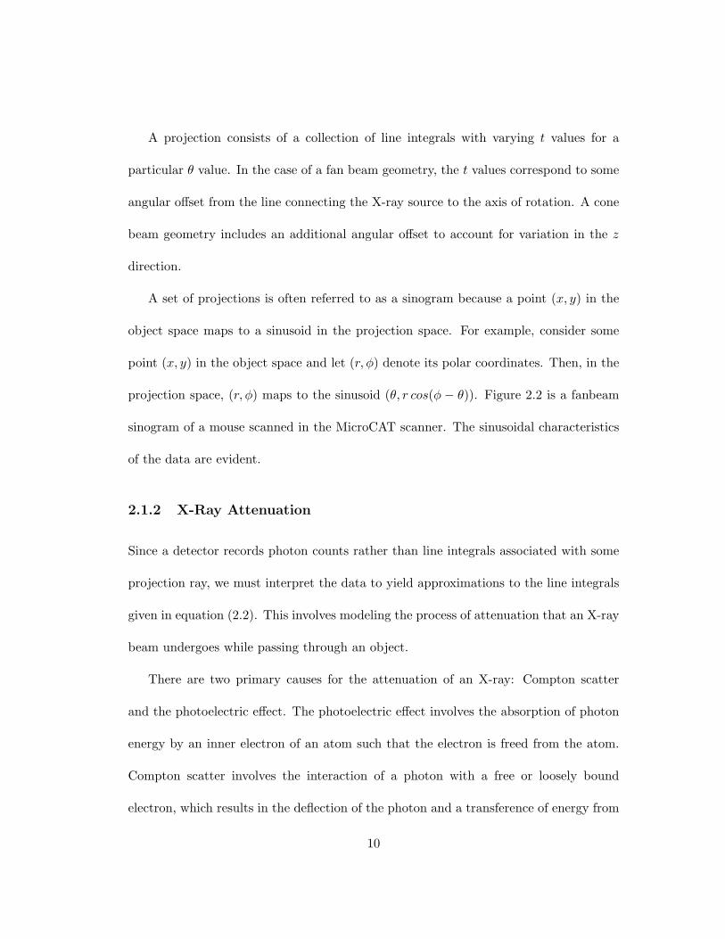
A set of projections is often referred to as a sinogram because a point (x, y) in the

object space maps to a sinusoid in the projection space. For example, consider some

point (x, y) in the object space and let (r, φ) denote its polar coordinates. Then, in the

projection space, (r, φ) maps to the sinusoid (θ, r cos(φ − θ)). Figure 2.2 is a fanbeam

sinogram of a mouse scanned in the MicroCAT scanner. The sinusoidal characteristics

of the data are evident.

2.1.2 X-Ray Attenuation

Since a detector records photon counts rather than line integrals associated with some

projection ray, we must interpret the data to yield approximations to the line integrals

given in equation (2.2). This involves modeling the process of attenuation that an X-ray

beam undergoes while passing through an object.

There are two primary causes for the attenuation of an X-ray: Compton scatter

and the photoelectric effect. The photoelectric effect involves the absorption of photon

energy by an inner electron of an atom such that the electron is freed from the atom.

Compton scatter involves the interaction of a photon with a free or loosely bound

electron, which results in the deflection of the photon and a transference of energy from

10

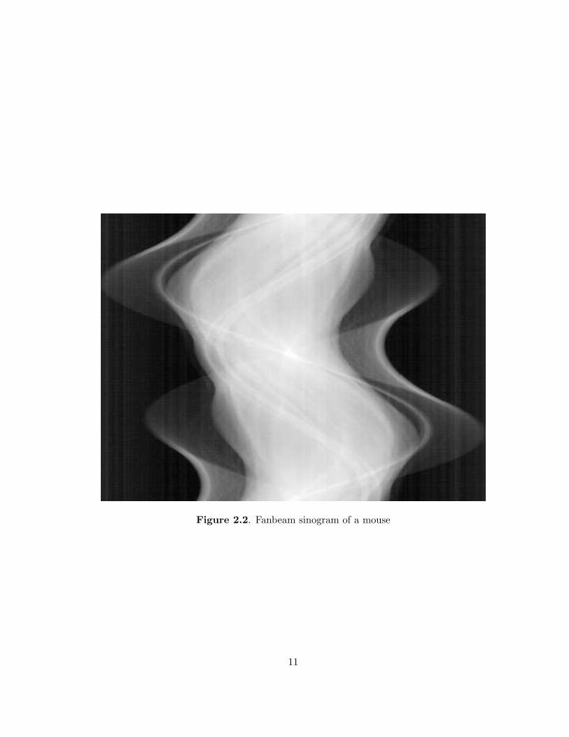
Figure 2.2. Fanbeam sinogram of a mouse

11

the photon to the electron. Most importantly for CT imaging, both of these effects are

dependent on the energy of the photon in question. Thus, attenuation is dependent on

the photon energy.

An X-ray beam is composed of photons with energies typically ranging between 20

and 150 keV for medical imaging purposes [6]. An X-ray source emits photons with en-

ergies in some range, which is dependent on the particular X-ray source. Unfortunately,

since the photon energies will be distributed throughout this range, the X-ray beam is

polychromatic. Since attenuation is dependent on the photon energy, and the X-ray

beam is polychromatic, precise modeling of the process of attenuation is very difficult.

Rather than attempting to model the attenuation in terms of polychromatic X-ray

beams, it is often assumed that the X-ray beams are monochromatic, or consisting only

of photons with equivalent energies. With this assumption, the model for attenuation

in the three dimensional case simplifies to [6]

Nd = N0 exp

{

−

∫

ray

µ(x, y, z)ds

}

(2.3)

where N0 is the number of photons emitted from the source, Nd is the number of photons

received at a detector cell, ray is the path joining the source and the detector cell, and

µ(x, y, z) is the attenuation map of the object at location (x, y, z). Furthermore, we can

rewrite equation (2.3) as

∫

ray

µ(x, y, z)ds = lnN0

Nd

. (2.4)

12

Comparing this to (2.1), it is evident that the line integral values are specified by

the right hand side of (2.4). Note that the N0 and Nd values will be known and that

the ray path can be approximated, so ln(N0/Nd) yields an approximation to the line

integral of µ(x, y, z) along the path described by ray.

Although the assumption of monochromatic X-ray energies simplifies the model for

attenuation, it can lead to artifacts in the reconstructions. Since objects tend to at-

tenuate lower energy photons more readily than higher energy photons, the effective

energy level of the X-ray beam is increased when passing through an object. This

phenomenon is known as beam hardening and leads to two primary reconstruction ar-

tifacts [6]. The first involves artificially high attenuation coefficients near the perimeter

of highly attenuating objects, such as bone. The second involves streaks near highly

attenuating objects. Researchers have proposed several techniques for eliminating the

beam hardening effects, but none are examined in this thesis.

Furthermore, although the preceding descriptions of the projection data are based

on line integrals, they do not accurately describe the geometry of a real scanner. Since

each detector cell has some area associated with it, the recorded photons travelled

through some three dimensional volume of the object rather than along a single line

before reaching the detector. We consider this discrepency when designing the system

models later in this chapter. Note that although the reading at a particular detector

cell involves some three dimensional path through the object, we refer to these paths as

projection rays throughout this thesis.

13

2.2 Representation as a Linear System

Let the object to be reconstructed be represented by f(x, y, z). Discretize this image

as a collection of N volumetric picture elements, or voxels, each of constant value.

This collection of voxels approximates the attenuation map of the object, and can be

represented in vector form as µ = (µ1, µ2, . . . , µN ). For the jth voxel, let µj represent

the constant value of the voxel. The goal of the reconstruction is now to assign values

to each of the voxels such that they approximate the true attenuation map as closely as

possible.

The data available to perform the reconstruction is the geometry and settings of

the scanner and the M projection readings. These projection readings originally take

the form of photon counts as indicated in equation (2.3), but we modify them to take

the form of equation (2.4). Let pi represent the ith such projection ray and let p =

(p1, p2, . . . , pM ) represent the collection of all projection rays over all view angles.

Relating the projection space to the voxel space requires the formation of a system

matrix, A, that accounts for the geometry of the scanner, modeling of the process of

attenuation, collimation, detector response, etc. This system matrix will have MxN

entries where aij quantifies the effect of the jth voxel on the attenuation of the ith

projection ray. Thus, the product Aµ translates from the voxel space to the projection

space, and AT p translates from the projection space to the voxel space. These operations

are known as forward projection and backprojection, respectively. Determining the

values of the system matrix plays a critical role in the reconstruction process and is

14

considered further in section 2.3.

Using the above terminology, we express the image reconstruction problem as the

linear system

Aµ + s = p (2.5)

where s accounts for scatter and other types of additive noise and distortion. For

the purposes of this thesis, we only model the scanner geometry and the process of

attenuation, so s is assumed to be zero. Given this system, we can apply various

techniques for solving linear systems to approximate the attenuation map of the object.

Note, however, that p typically includes noise and that µ is subject to a nonnegativity

constraint since a negative value would physically correspond to a portion of the object

that increases rather than decreases the number of photons in the X-ray. These facts

should be considered when choosing a reconstruction algorithm. Several reconstruction

algorithms are presented in chapter 3.

2.3 Modeling Techniques

The quality of the system matrix A has a substantial impact on the accuracy of the

reconstruction. Although ideally the entry aij should fully quantify the effect of voxel

j on projection ray i, creating a matrix of this form is seemingly computationally pro-

hibitive. Thus, we pursue techniques to acceptably approximate these ideal values in a

15

computationally feasible fashion.

2.3.1 Ideal Model

Consider the transmission energy that is collected at a single detector cell. To determine

the path through which the X-rays traveled to reach this detector, connect the perimeter

of the detector cell back to the X-ray source to form the contributing volume. Now, the

entry aij is the volume of the intersection between voxel j and the path corresponding

to the ith projection ray.

Note that even the above includes simplification of the scanner geometry. In reality,

the source is not a point source. Rather, it has some nonzero area. However, finding

the volumes to fit even the slightly simplified model above is a significant computa-

tional burden. Doing so would involve finding the volumetric intersection of a three

dimensional path with a potentially large set of voxels. This operation would have to

be repeated for each detector cell and for each view angle.

Fortunately, there are simplified techniques for constructing the system matrix which

produce acceptable results with much more manageable computational requirements.

2.3.2 Single Line Intersection Model

Rather than the entire three dimensional path, consider only the line which joins the

X-ray source to some point in the detector cell, such as the center of the detector

cell. Computing the intersection of this sample line with each voxel yields a rough

approximation of that voxel’s contribution to the attenuation of the energy collected

16

at the detector cell. This is depicted in figure 2.3 where wj denotes the length of the

intersection with the jth voxel. Note, however, that the consideration of only one line

will not include all of the voxels that actually contributed to the attenuation of the

energy collected at the detector cell since a single line cannot represent the full volume

of a given path. Additionally, the relative weights of each voxel will not be the same as

in the ideal case, which further compromises the validity of a single line based model.

The attractive aspect of this modeling approach is the computational ease of finding

the line intersections. An efficient method of computing these intersections was proposed

by Siddon [13] and later improved by Jacobs et al. [5]. The basic premise of the fast

radiological path calculation involves iteratively stepping along the projection ray, which

is represented parametrically, to find each of the intersection points with the pixel or

voxel space. First, represent the projection ray as

p = s + α(d − s) (2.6)

where p is some point along the line, s is the source point, and d is the destination

point. Each of p, s, and d is a vector containing the x, y, and z coordinates of the

points in the three dimensional scanner coordinate system. We first calculate the α

values corresponding to entering and exiting the voxel space. We then calculate the

number of x, y, and z planes intersected by this line in the voxel space. Based on this

information, we can iteratively step through the α values corresponding to intersections

with the voxels and calculate the distances associated with these intersections.

17

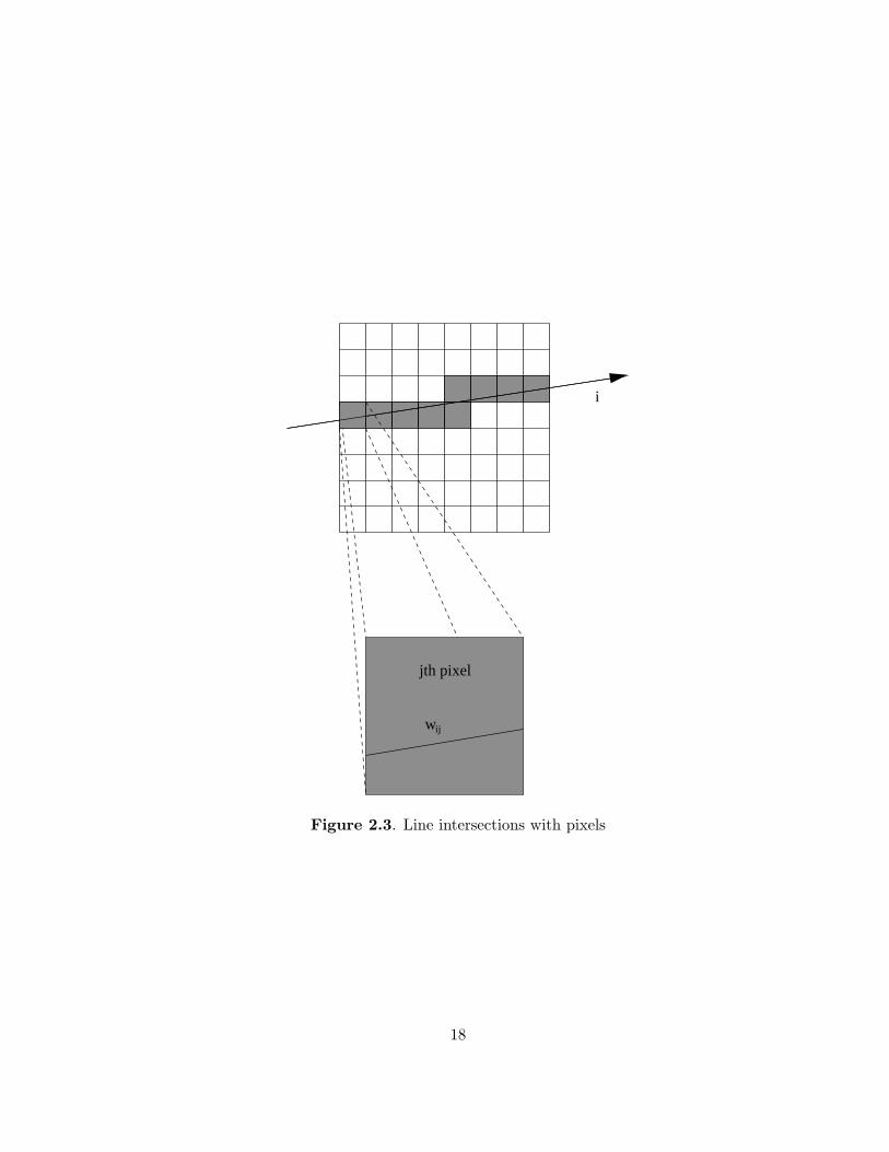
wij

i

jth pixel

Figure 2.3. Line intersections with pixels

18

Unfortunately, the use of line intersections yields serious artifacts in the reconstruc-

tions. The most significant of these artifacts takes the form of rings in the reconstructed

images. These are due to interference patterns emerging from the conebeam geometry.

We analyze the causes and effects of these artifacts more thoroughly in the results

section. This phenomenon was previously noted and explained by Zeng and Gullberg

[16].

2.3.3 Multiple Line Based Model

One method of mitigating the ring artifacts produced by the single line based models is

using multiple sample lines per detector cell rather than a single line. After computing

the line intersections for each of the chosen lines, the intersection values for each voxel

can be averaged to yield a single row in the system matrix.

Assuming the sample lines are chosen in a reasonable fashion, the likelihood of

including each voxel that contributed to the attenuation of a given ray grows as the

number of sample lines increases. Furthermore, the relative weights for each voxel

should approach the true values as the number of sample lines increases. Thus, the

quality of the system model should increase as the number of sample lines increases. Of

course, the computational burden of computing the system matrix also increases with

the number of sample lines. The results section includes a more quantitative analysis

of the multiple line based model using varying number of lines per detector cell.

19

2.3.4 Trilinear Interpolation Model

The trilinear interpolation model is based upon a significantly different approach than

the volume or line based techniques mentioned in the above sections. The following

development is the three dimensional equivalent of the two dimensional interpolation

based scheme introduced in [6]. The general idea of the trilinear interpolation model is

to segment the projection ray into points, calculate the relative contributions of the eight

closest voxel centers to each of these points, and sum the contributions to approximate

the system matrix values. Note that the physical interpretation of these values is not

as clear as the line intersection based models. This causes some data scaling issues that

we address in the results section.

To more formally specify the trilinear interpolation model, first express the relation-

ship between the attenuation map µ(x, y, z) and the projection data as

pi = Riµ(x, y, z) =

∫ ∞

−∞

∫ ∞

−∞

∫ ∞

−∞

µ(x, y, z)δ(ri(x, y, z)) dx dy dz (2.7)

where ri(x, y, z) = 0 represents the equation of the ith ray and Ri is the projection op-

erator along the ith ray. The goal is to approximate the true attenuation map µ(x, y, z)

as closely as possible with a discretized attenuation map. This discrete attenuation map

requires a choice of basis functions bj(x, y, z).

Assume the basis functions are chosen and using N of them yields an acceptable

20

approximation to µ(x, y, z). Based on these assumptions, we have

µ(x, y, z) ≈

N∑

j=1

gjbj(x, y, z) (2.8)

where gj ’s are the coefficients of expansion representing µ(x, y, z) relative to the basis

set bj(x, y, z). Using substitution, the forward projection process can be written as

pi = Riµ(x, y, z) ≈N

∑

j=1

gjRibj(x, y, z) =N

∑

j=1

aijgj (2.9)

where aij represents the line integral of bj(x, y, z) along the ith ray. Note that if a

pixel basis is chosen for bj(x, y, z), this model simplifies to the line intersection based

approach above.

However, for the trilinear interpolation approach, trilinear basis elements are chosen

instead. These basis functions offer support over eight voxels. We approximate the ray

integral over Riµ(x, y, z) by a finite sum over a set of Mi equidistant points µ(sim), for

1 ≤ m ≤ Mi, by

pi ≈

Mi∑

m=1

µ(sim)∆s (2.10)

where ∆s is a step size and µ(sim) is calculated from the values gj of µ(x, y, z) on the

21

eight nearest voxels centers by trilinear interpolation. We write this as

f̂(sim) =

N∑

j=1

dijmgj (2.11)

for m = 1, 2, · · · , Mi. Thus, dijm is the contribution of the jth voxel to the mth point

on the ith ray. Substituting (2.11) into (2.10) yields

pi =

mi∑

m=1

N∑

j=1

dijmgj∆s =N

∑

j=1

aijgj (2.12)

where the coefficients aij are defined as the sum of the contributions by the jth voxel

to the ith ray along all of the sample points of the ray. Thus,

aij =

Mi∑

m=1

dijm∆s. (2.13)

In the present implementation, we store the aij values from equation (2.13) in the

system matrix. Furthermore, we choose equidistant sample points along the line con-

necting the X-ray source to the center of a given detector cell and set the step size, ∆s,

to half the width of a voxel as recommended by Kak and Slaney [6]. We can then use

the resulting system matrix just as we would for the single and multiple line intersection

models.

One aspect of the trilinear interpolation technique worthy of note is that some

voxels that made no contribution to the attenuation of a given ray may be included

22

as a contributing voxel for that ray. This could occur when one or more of the eight

neighboring voxel centers of a sample point µ(sim) corresponds to a noncontributing

voxel. In these cases, a smoothing or blurring of the reconstructed image will occur,

although it is difficult to quantify the extent of this blurring. Also, this side effect may

be desirable.

23

Chapter 3

Survey of Algorithms

We can subdivide the class of iterative algorithms used for image reconstruction into

algebraic and statistical algorithms. From the class of algebraic reconstruction algo-

rithms, we chose to implement the Simultaneous Algebraic Reconstruction Technique

(SART) [6]. The statistical algorithms implemented include Expectation Maximization

(EM) [12], [7] and a Weighted Least Squares (FWLS) reconstruction technique proposed

by Fessler [2]. We present each of these algorithms in this chapter.

3.1 Algebraic Reconstruction Techniques

The only algebraic reconstruction algorithm implemented in this thesis is SART, al-

though several others exist, such as the Algebraic Reconstruction Technique (ART) and

the Simultaneous Iterative Reconstruction Technique (SIRT). Of these three, however,

SART is the most sophisticated and fits nicely into the developed framework.

24

3.1.1 Algebraic Reconstruction Preliminaries

This development of the algebraic reconstruction techniques follows closely from the ap-

propriate material in [6]. Recall from section 2.2 that we can express the reconstruction

problem as the linear system

Aµ = p, (3.1)

where aij is the contribution of the jth voxel to the attenuation of the ith projection

ray, µj is the value of the jth voxel, and pi is the ith projection ray. We compute the

system matrix A using the techniques discussed in chapter 2.

Assume that p contains M projection rays and µ contains N voxels. Therefore, the

image represented by µ is a point in an N -dimensional voxel space and the M equations

described by the linear system represent hyperplanes in this voxel space. If a unique

solution to the linear system exists, then these hyperplanes intersect at a single point

in the voxel space that represents this unique solution. However, since the system is

generally over determined (M > N) or underdetermined (M < N) and noise is included

in the projection data, the linear system does not contain a unique solution. Thus, we

must consider convergence properties for proposed algebraic reconstruction algorithms.

The technique at the heart of the algebraic reconstruction algorithms is the “method

of projections” introduced by Kaczmarz. First, take an initial guess,

µ(0) = (µ(0)1 , µ

(0)2 , · · · , µ

(0)N ), (3.2)

25

where µ represents one point in the N -dimensional voxel space. Project this guess onto

the first hyperplane described in the linear system, then reproject the resultant point

onto the second hyperplane described by the linear system, and so on. Projecting onto

the Mth hyperplane completes the first iteration and this process is continued until the

solution is acceptable. We can mathematically describe this process by

µ(i) = µ(i−1) +(pi − µ(i−1) · ai)

ai · aiai (3.3)

where µ(i) is the approximation after performing i projections, · represents a dot product,

and ai is the ith row of A, or ai = (ai1, ai2, · · · , aiN ). Note that M projections are

required to complete a full iteration, so kM projections are required for k iterations.

If a unique solution exists, this series of projections is guaranteed to converge to

the solution. It has been shown that in the case of an overdetermined system, the

approximated solutions will oscillate around the neighborhood of the intersections of the

hyperplanes. Furthermore, it has also been shown that in the case of an underdetermined

system, (3.3) converges to a solution, f ′, that minimizes |f (0) − f ′|.

3.1.2 SART

The Simultaneous Algebraic Reconstruction Technique (SART) includes a modification

to the update equation that allows an averaged voxel update after all of the projec-

tions are considered rather than after each projection ray. Since we implemented the

algorithms using the Message Passing Interface (MPI) for parallel load distribution, the

26

aggregated update technique is highly advantageous as it requires less communication

overhead. Furthermore, we can implement the aggregate updates using forward and

backprojections of the system matrix which fits nicely into the developed framework.

The alternate update technique used in SART yields the following update for each voxel

after the kth iteration:

µ(k+1)j = µ

(k)j +

∑

i

[

aijpi−ai·µ

(k)∑

j aij

]

∑

i aij. (3.4)

To be used in the current framework, we need to express this algorithm in terms of

a linear system using forward and backprojections. Let vectors R and C represent the

row and column sums of A, respectively, so Ri =∑

j aij and Cj =∑

i aij . Then we can

express equation (3.4) as

µk+1 = µk + {AT [(p − Aµk) � R]} � C (3.5)

where � represents element-wise division. Thus, each iteration of SART requires one

forward projection and one backprojection.

One additional modification proposed for SART is the heuristic application of a

Hamming window to each projection ray. The inclusion of the Hamming window em-

phasizes the central portions of each projection ray and has been experimentally shown

to improve the reconstruction quality. However, including the Hamming window yields

a proliferation in the number of elements that must be stored. Thus, since storage is a

27

major consideration for the iterative framework, we did not employ a Hamming window

modification.

3.2 Statistical Reconstruction Techniques

The class of statistical reconstruction techniques covered in this thesis includes Ex-

pectation Maximization (EM) and a Weighted Least Squares (FWLS) reconstruction

algorithm. Whereas the algebraic techniques evolve directly from an algebraic interpre-

tation to a linear system, the statistical techniques are founded in a statistical context

with solution techniques representable as a linear system.

3.2.1 Expectation Maximization

The expectation maximization (EM) algorithm for emission tomography was proposed

by Shepp and Vardi [12]. Shortly thereafter, it was independently proposed by Lange

and Carson, who extended it to transmission tomography [7]. Previous to the work

related to computed tomography, an EM algorithm was proposed by Richardson [11]

and Lucy [8] for use in the realm of astronomy.

For the purposes of this thesis, we implement the emission EM algorithm rather

than the transmission algorithm. This is due to the relative ease with which the emis-

sion algorithm fits into the linear system based framework that we have developed.

On the other hand, the implementation of the transmission algorithm using the linear

system framework is seemingly more difficult. In particular, the transmission model

28

introduces a proliferation of new variables which cannot be modeled using forward and

backprojections. Usage of the emission EM algorithm for transmission reconstruction

is also documented by Wang in [15]. The following development follows closely to the

development in [7].

The goal of emission CT is to approximate the photon emission intensities of some

object. As with transmission CT, the object is represented as a collection of voxels.

Let λj denote the average source intensity for voxel j and bij represent the probability

that a photon leaving voxel j reaches the ith projection detector. Furthermore, let ∆ti

denote the length of the aquisition time for projection i and let cij = bij∆ti. Note the

similarities between the λj and cij quantities in the emission case and the µj and aij

values in transmission case.

Let Xij be the random number of photons that are emitted by voxel j and contribute

to projection i. Then the mean of Xij is cijλj . Furthermore, let Yi represent the total

number of photons recorded for the ith projection. Thus,

Yi =∑

j

Xij . (3.6)

As shown in [7], Xij and Yi are both Poisson distributions. The Yi values represent

the recorded data and are shown above to be functions of the Xij data values. Thus,

Xij represents a complete but unobserved set of data from which Yi can be derived.

The EM algorithm works by increasing the log likelihood of the observed data with

respect to the current estimation of the source intensity values at each iterative step.

29

This process involves two steps: an E-step, which forms a conditional expectation, and

an M-step, which involves maximizing the conditional expectation to give new source

intensity estimations.

Using the above definitions, the E-step can be formulated as

E(ln f(X, λ)|Y, λn) =∑

i

∑

j

{−cijλj + Nijln(cijλj)} + R, (3.7)

where f(X, λ) is the density function of X, λn is the current estimation of the source

intensity values, R is independent of the new λ, and Nij is given by

Nij = E(Xij |Yi, λn) =

cijλnj Yi

∑

k cikλnk

. (3.8)

The M-step is implemented by taking the partial derivatives of (3.8) with respect to

λj , setting them to zero, and solving to get the following update equation:

λn+1j =

λnj

∑

i cij

∑

i

cijYi∑

k cikλnk

. (3.9)

Note that if the initial source intensity estimation, λ0, is nonnegative in (3.9), then

each subsequent λn will be nonnegative as well. This is a highly desirable feature of the

EM algorithm as the physical aspect of attenuation, or source intensity in the emission

case, imposes a non-negativity constraint on a reasonable solution.

In order to use update equation (3.9) in the current framework, it must be stated

30

in terms of a linear system using forward and backprojection operations. To do this,

let C = [cij ], λ = [λj ], and Y = [Yi]. The scaling factor represented by∑

i cij is simply

a vector of column sums that can be computed by backprojecting C over a vector of

ones. Denote this set of column sums as S. The term

∑

i

cijYi∑

k cikλnk

(3.10)

is equivalent to CT (Y � Cλn) where � represents element-wise division and matrix

multiplication has the highest priority in the order of operations. Thus, the entire

update algorithm can be stated as

λn+1 = (λn ⊗ CT (Y � Cλn)) � S (3.11)

where ⊗ and � represent element-wise operations as before.

However, (3.11) is still in terms of the emission case. To use this for the transmission

case, replace C, λ, and Y by A, µ, and p, respectively. Recall that A = [aij ] represents

the effect of voxel j on the attenuation of projection ray i, µ = [µj ] is the attenuation

coefficient of voxel j, and p = [pi] is the detector reading for projection ray i. Note

that while this development of EM does not directly model the transmission case, the

interpretations of the substituted and original values are similar in each case.

31

Using these substitutions, the EM algorithm used in this thesis is given by

µn+1 = (µn ⊗ AT (p � Aµn)) � S (3.12)

where Sj is now∑

i aij .

3.2.2 Weighted Least Squares

The last reconstruction technique implemented for this thesis is a Weighted Least

Squares (FWLS) technique described by Fessler [2]. The following presentation mim-

ics that development closely. As presented, this model assumes that the X-ray beams

are monoenergetic. In the referenced paper, this model was extended to work with

polyenergetic X-ray beams, but that work was not implemented in this thesis.

Recall from equation (2.3) that attenuation in the monoenergetic case can be rep-

resented by

Nd = N0 exp

{

−

∫

ray

µ(x, y, z)ds

}

(3.13)

where N0 is the source energy, µ(x, y, z) is the attenuation map for the object, ray is

some projection ray, and Nd is the resultant energy after attenuation. For notational

convenience, we rewrite this equation as

Yi = Ii exp

{

−

∫

Li

µ(x, y, z)ds

}

(3.14)

32

where Yi is now interpreted as the detector reading for the ith projection ray, Ii is the

source energy for the i projection ray, and Li is the path of the ith projection ray.

Now, assume the following statistical model for the projection measurements:

pi ∼ Poisson{bi exp−[Af ]i +ri}, i = 1, . . . , N (3.15)

where bi is the blank scan factor, ri is a noise correction factor accounting for background

events and projection read-out noise variance, A is the system matrix discussed in

chapter 2, [Af ]i =∑p

j=1 aijfj is the ith line integral, and N is the number of measured

rays. We determine the blank scan factor values by performing a partial scan with no

objects located in the scanner. These values can then be used as a close approximation to

the Ii values in equation (3.14). We determine the noise correction factor by performing

a scan with the X-ray source blocked to determine a baseline reading for the scanner

environment. Thus, the aij , bi, and ri values are all known before commencing the

reconstruction.

The reconstructed image, f , can be approximated by maximizing the following Pois-

son log-likelihood:

L(f) =N

∑

i=1

{Yi log(bie−[Af ]i + ri) − (bie

−[Af ]i + ri)}. (3.16)

To help prevent noisy data from yielding a poor reconstruction, a regularization term

can be added to (3.16) to enforce a known structure of the object on the reconstructed

33

image. For example, since adjacent voxels should generally have similar values, the

regularization term can penalize differences in the values of neighboring voxels. However,

we did not explore penalties in this thesis. Adding a non-negativity constraint, the goal

of the reconstruction is now:

f̂ = argmaxf≥0

L(f). (3.17)

To develop an iterative algorithm, first rewrite (3.16) as

−L(f) =N

∑

i=1

gi([Af ]i), (3.18)

where

gi(l) = −Yilog(bie−l + ri) + (bie

−l + ri). (3.19)

Applying a second order Taylor expansion to gi(l) around an estimate l̂i of the line

integral yields the following approximation:

gi(l) ≈ gi(l̂i) + g′i(l̂i)(l − l̂i) +g′′i (l̂i)

2(l − l̂i)

2. (3.20)

Assuming Yi > ri, the line integral can be estimated as

l̂i = log(bi

Yi − ri). (3.21)

34

Substituting the estimate for l̂i into (3.20) yields

gi(l) ≈ (Yi − Yi log Yi) +wi

2(l − l̂i)

2 (3.22)

where wi is defined by

wi =

(Yi−ri)2

Yi, Yi > ri

0, Yi ≤ ri.

(3.23)

Since the first term in (3.22) is independent of l, it can be dropped. Substituting

(3.22), with the first term dropped, into (3.18) yields the following FWLS cost function:

L(f) =N

∑

i=1

wi

2([Af ]i − l̂i)

2. (3.24)

Rather than minimizing L(f), it can be replaced by a surrogate function φ(f ; fn) that

is easier to minimize. The surrogate function chosen in [2] is

φ(f ; fn) =N

∑

i=1

p∑

j=1

αijwi

2

(

aij

αij(fj − fn

j ) + [Afn]i − l̂i

)2

(3.25)

where

αij =aij

∑pj=1 aij

. (3.26)

35

Setting the first derivative of φ(f) to zero yields the following update equation:

fn+1j =

fnj −

∑Ni=1 aijwi([Afn]i − l̂i)

∑Ni=1

a2ijwi

αij

+

, j = 1, . . . , p, (3.27)

where []+ enforces nonnegativity by setting fn+1j to zero if the above equation produces

a negative number.

In our implementation, µ and p are substituted for f and Y , respectively. While we

used our typical forward projector for the line integral approximation, [Afn]i, we used

a specialized backprojector for the backprojection operation due to the extra weighting

terms.

36

Chapter 4

Managing the System Matrix

The most significant hurdles to overcome when implementing the iterative reconstruc-

tion algorithms are the potentially massive size of the system matrix and the compu-

tational time required to perform operations using the system matrix. One option is

to recompute the system matrix values during each iteration rather than storing them.

While this approach mitigates the storage requirements, it results in a significant du-

plication of computation since the system matrix remains the same for each iteration.

If many iterations are requested or the system modeling technique is complicated, this

could result in a significant increase in total computation time. Thus, instead of pursuing

this option, we developed and employed techniques to reduce the storage requirements

of the system matrix. We introduce these techniques in the following sections.

37

4.1 Explicit Storage

The most direct approach for representing the system matrix involves explicitly storing

each matrix value. Using this approach would require P × Dy × Dz rows and Nx ×

Ny ×Nz columns, where P is the number of projection rays, Dy and Dz are the number

of detector cells in the y and z directions, respectively, and Nx, Ny, and Nz denote

the dimensions of the voxel space in the x, y, and z directions, respectively. Even

for a relatively small scanner equipped with a 256 × 256 detector, operating over 360

projections, and for which we reconstruct a 256×256×256 volume, explicit storage would

require approximately 400 trillion entries. If we use four byte floating point numbers

for each entry, the storage requirements would be approximately 1.6 petabytes, or 1600

terabytes. Many scanners have larger detectors, acquire data for more view angles, and

require larger image volumes to be reconstructed. Clearly, explicit storage is far too

simplistic an approach.

4.2 Sparse Storage

Recall that a nonzero entry aij in the system matrix denotes that the jth voxel affected

the ith projection ray based on a given system model. Thus, with most system models,

the vast majority of the entries in the system matrix are zero since a given ray intersects

only a small portion of the object. In other words, the system matrix is sparse. While

the density of the system matrix depends on the specific modeling technique utilized, it

is typically less than 0.001% for the conebeam geometries considered here.

38

For the purposes of this thesis, we employed the compressed row storage technique

for sparse matrix storage [1]. This method requires three vectors: a row pointer vector,

a value vector, and a column index vector. Denote these vectors by ~r, ~v, and ~c, respec-

tively. The vectors ~v and ~c each have one entry for every nonzero in the matrix. The

vector ~r has size M + 1, where M is the number of projection rays. Four byte integers

are used for each entry in ~c and ~r, and four byte floating point numbers are used for

each entry of ~v.

Each of the column indices in ~c must encode the i, j, and k indices for a given voxel.

We compute the column indices as

c = i + jNx + kNxNy (4.1)

where c is a column index, and i, j, and k represent the voxel indices in the x, y, and

z direction, respectively. We can then recover the original i, j, and k values using

i = c % Nx (4.2)

j = (c % NxNy)/Nx (4.3)

k = c/(NxNy) (4.4)

where % denotes the modulo operator and the divisions for j and k are integer divisions.

Due to performance issues, we did not perform the column index decoding as above,

although our implementation is functionally equivalent. Instead, we take advantage of

39

the fact that adjacent entries in a row of the matrix often represent adjacent voxels and

thus require an update to only a single voxel index. Note that encoding i, j, and k using

a four byte integer restricts the voxel space to having a maximum of 232 voxels. While

this limit is sufficiently large for the reconstructions performed in this thesis, larger

reconstructions would require more voxels, with a corresponding increase in storage

requirements.

4.3 System Symmetries

Due to the circular scanning geometry, there are certain symmetries that we can exploit

to prevent storing significant portions of the matrix. In fact, exploiting these symmetries

reduces the storage requirements by approximately a factor of eight. In the following

subsections, we describe the nature of these symmetries for the two dimensional case

and then generalize to the three dimensional case.

4.3.1 Overview of Symmetries

The basis of the symmetries can be explained rather simply for the continuous case.

The X-ray source follows a circular path around the object as it generates projections.

This scanning circle can be subdivided into eight octants as shown in figure 4.1. By

reflecting a projection ray from octant one, say SD, to each of the remaining octants, we

generate several additional projection rays that are symmetric to SD. These symmetric

projection rays are depicted in figure 4.2. Thus, by storing only the portion of the system

40

32

67

8

1 4

5

Figure 4.1. Scanning circle octants.

SD

Figure 4.2. All symmetries of SD.

matrix corresponding to the projection rays originating in octant one, we can generate

the corresponding projection rays for the remaining seven octants. This significantly

reduces the storage requirements for the system matrix.

4.3.2 Mathematical Formulation of Symmetries

Consider a scanning circle with radius r that is centered at the origin of the coordinate

system. Let the X-ray source, S, lie at some point (x, y) along the first octant of the

scanning circle. Then a projection ray emitted from S will intersect some other point

on the scanning circle, say D = (x′, y′). This is depicted in figure 4.3. Now, reflect the

line segment SD about the line y = −x, which separates the first and second octants of

the scanning circle. The points S and D reflect to S′ = (−y,−x) and D′ = (−y′,−x′),

respectively. This is illustrated in figure 4.4. Continuing this procedure to get sources

in each of the eight octants yields the lines shown in figure 4.2.

In order to relate these observations to the fan beam scanner geometry, it is useful

41

S = (x,y)D = (x’,y’)

Figure 4.3. Projection ray SD (points).

S = (x,y)

D’ = (−y’, −x’)

S’ = (−y,−x)

D = (x’,y’)

Figure 4.4. Reflection of SD (points).

to represent the line segment SD in terms of a view angle and fan angle. Label the line

connecting the X-ray source to the origin as SO. Then the view angle, θ, of projection

source S is simply the angle between the negative x-axis and SO. Furthermore, the

fan angle, φ, is the angle between SD and SO. We illustrate these angles in figure 4.5.

Performing the same reflection operation as before yields S′D′ with view angle θ′ and

fan angle φ′ as shown in figure 4.6. It can be easily verified using similar triangles that

θ′ = π/2 − θ and φ′ = −φ.

We introduce the notation l1 = (θ, φ) to denote a projection ray, l1, with view angle

θ and fan angle φ. We have shown above that reflecting l1 = (θ, φ) about the line

y = −x yields l2 = (π/2 − θ,−φ). These two lines are symmetric in the sense that

we can generate one using the other. Continuing the process of reflection to generate

projection rays in each of the eight octants yields the results summarized in table 4.1.

42

SD

φ

θO

Figure 4.5. Projection ray SD (angles).

O

D’

S’D

S

’θ

’φ

Figure 4.6. Reflection of SD (angles).

Table 4.1

Symmetries based on reflection

Line before reflection Reflected about Line after reflection

l1 = (θ, φ) y = −x l2 = (π/2 − θ,−φ)l2 = (π/2 − θ,−φ) x = 0 l3 = (π/2 + θ, φ)l3 = (π/2 + θ, φ y = x l4 = (π − θ,−φ)l4 = (π − θ,−φ) y = 0 l5 = (π + θ, φ)l5 = (π + θ, φ) y = −x l6 = (3π/4 − θ,−φ)l6 = (3π/4 − θ,−φ) x = 0 l7 = (3π/4 + θ, φ)l7 = (3π/4 + θ, φ) y = x l8 = (2π − θ,−φ)

43

4.3.3 Limitations of Symmetries

Unfortunately, the usage of symmetries imposes some restrictions on the scanner settings

and geometry. The first restriction is that projection angles must be distributed such

that any angle not in the first octant has an angle symmetric to it in the first octant. The

second is that the detector must be centered about the line connecting the X-ray source

to the axis of rotation. In other words, the detector cannot have an offset associated

with it.

The first restriction is easily overcome by specifying the scanning parameters such

that no inconsistencies occur. Choosing view angles that uniformly divide the scanning

circle accomplishes this. The second restriction is difficult to prevent at the hardware

level, but we can process the acquired projection data to compensate for the offset. In

this work, we use linear interpolation to rebin the data such that it satisfies the above

centering constraint. This involves ignoring some of the data from the edges of the

detector, but allows us to employ the symmetry techniques.

While not a limitation, it should also be noted that the projections corresponding

to θ = 0 and θ = π/4 are special cases. Each of those projections can only be reflected

to yield projection rays for three additional projections rather than seven. For example,

θ = 0 is only symmetric to π/2, π, and 3π/2. Since θ = 0 is not symmetric to θ = π/4

by reflection about any of the lines given above, both projections must be stored if in

the original projection data set. Therefore, assuming that 360 projections are taken

uniformly over the scanning circle, data for the first 46 projections must be stored,

44

yielding a reduction in storage by nearly a factor of 8.

4.3.4 Implementation of Symmetries

We will now associate these observations regarding symmetries with the storage of

values in the system matrix. Assume that the line intersection based system described

in section 2.3.2 is implemented for the two dimensional case. First, the area inside

the scanning circle is divided into a grid of pixels, which is centered about the origin.

The row of the system matrix corresponding to some line segment with its source in

the first octant, say l1, would contain the length of intersection of l1 with each pixel.

Since the pixel grid is centered and reflection maintains length, two intersection points

of one pixel will reflect to two intersection points of another pixel, and the length

between those points will be identical. Thus, a symmetric projection ray has identical

intersection lengths with the pixel grid as l1. Once determining the mapping of pixel

indices that must be carried out during reflection, we can compute the full system matrix

by storing only the portion where the X-ray source lies in the first octant. Therefore,

by storing only a small subset of the system matrix, we compute the entire system

matrix without recalculating the intersection values. Note that since these are three

dimensional reconstructions, we use voxels instead of pixels, but the concept remains

the same.

More generically, a row in the system matrix is a collection of weights corresponding

to the contribution of a particular voxel to the attenuation of a projection ray. Each of

these values has an index from which we can determine the three voxel indices i, j, and

45

k, that correspond to the x, y, and z directions, respectively. We offered one potential

implementation of this index decoding in (4.2).

The voxel space has dimensions Nx, Ny, and Nz in the x, y, and z directions,

respectively, and indexing for the voxels begins at zero. Thus, for example, possible i

values are 0, 1, . . . , Nx − 1. Given a row of indices, generating the matrix row for a ray

that is symmetric to the given row simply involves changing the voxel indices based on

the octant containing the source of the symmetric ray. These voxel index changes are

given in table 4.2. This table gives the conversion for voxel indices (i, j, k) corresponding

to a projection ray with its source in octant one to voxel indices (i′, j′, k′) corresponding

to a symmetric projection ray.

This allows for the following implementation. We store the intersection data for any

projection ray that has the X-ray source in the first octant of the scanning circle. We

also provide a method to request a specific row of the matrix, which may or may not be

stored. If the row is stored, we simply return it. Otherwise, we determine the row that

represents the ray in the first octant symmetric to the row being requested. We can

then construct the requested matrix row from the stored row by the given index changes

and return it to the caller. To improve the efficiency of these operations, we compute

and use all of the projection rays symmetric to a given ray at the same time. Otherwise,

we must decode the column indices for the stored rays more than is necessary.

46

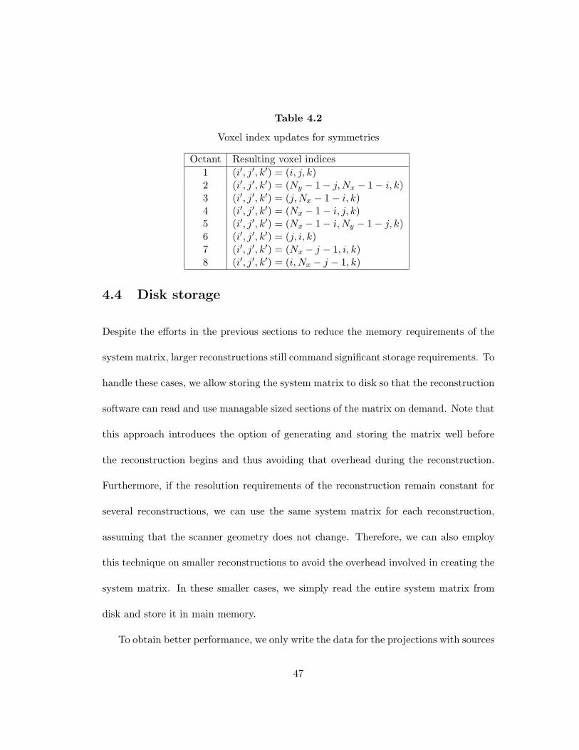
Table 4.2

Voxel index updates for symmetries

Octant Resulting voxel indices

1 (i′, j′, k′) = (i, j, k)2 (i′, j′, k′) = (Ny − 1 − j, Nx − 1 − i, k)3 (i′, j′, k′) = (j, Nx − 1 − i, k)4 (i′, j′, k′) = (Nx − 1 − i, j, k)5 (i′, j′, k′) = (Nx − 1 − i, Ny − 1 − j, k)6 (i′, j′, k′) = (j, i, k)7 (i′, j′, k′) = (Nx − j − 1, i, k)8 (i′, j′, k′) = (i, Nx − j − 1, k)

4.4 Disk storage

Despite the efforts in the previous sections to reduce the memory requirements of the

system matrix, larger reconstructions still command significant storage requirements. To

handle these cases, we allow storing the system matrix to disk so that the reconstruction

software can read and use managable sized sections of the matrix on demand. Note that

this approach introduces the option of generating and storing the matrix well before

the reconstruction begins and thus avoiding that overhead during the reconstruction.

Furthermore, if the resolution requirements of the reconstruction remain constant for

several reconstructions, we can use the same system matrix for each reconstruction,

assuming that the scanner geometry does not change. Therefore, we can also employ

this technique on smaller reconstructions to avoid the overhead involved in creating the

system matrix. In these smaller cases, we simply read the entire system matrix from

disk and store it in main memory.

To obtain better performance, we only write the data for the projections with sources

47

in the first octant of the scanning circle to disk. We compute the remaining data using

the system symmetries. Furthermore, by using two threads to perform these operations,

the system naturally staggers itself such that one thread can be interpreting and using

the data while another reads data from the disk. After completing their respective

tasks, these threads switch roles. This implementation reduces the ultimate impact on

performance. We include timing information regarding the impact of the disk reads in

the results section.

4.5 Implementation Issues

4.5.1 Spherical Support Region

A scanner provides data support for some location if projection data is available for

that location for some view angle. Recall that the conebeam geometry emits X-rays

from the source in a cone shape as it rotates around the scanning circle. Intersecting

the cones over all possible view angles yields a spherical region in the scanning area for

which the scanner provides full data support. We refer to this region as the spherical

support region (SSR). Since voxels located outside of the SSR lack full data support,

we do not include them in the system matrix. This prevents unnecessarily allocating

storage or computational resources to reconstruct these voxels.

48

4.5.2 Multi-Threading

Since we typically run the reconstructions on machines with more than one processor,

being able to harness the additional processors is advantageous. In this project, we

distribute both the forward and backprojectors across the available processors using

POSIX threads. This distribution is accomplished by simply assigning to each of the n

processors 1/n of the data available for each projection.

4.5.3 Load Distribution via MPI

Due to the potential size and computational burden of the presented iterative recon-

struction procedures, it is highly beneficial to distribute the storage and computational

requirements to a cluster of machines. We perform this distribution using the LAM/MPI

implementation version 6.5.8.

Distributing the System Matrix

Since the total storage requirements are dominated by the system matrix, the largest

storage savings will result from distributing this system matrix as equally as possible

across all of the cluster nodes. We accomplish this by assigning certain projections

to each node. First, we determine the total number of projections to store based on

the number of view angles and the symmetry setting. If the number of MPI hosts

evenly divides the number of projections to store, then we assign an equal number of

projections to each MPI host. Otherwise, we distribute the projections as equally as

49

possible, although some hosts will get one more projection than some of the others.

Since the hosts must frequently share data during the iterative reconstructions,

which requires all of the hosts to be at an equivalent stage of the computation, an

unequal load distribution will force some hosts to wait idly on others. We generally

avoided this situation during the test runs by ensuring that the number of MPI hosts

evenly divided the number of projections to store.

The implementation of the forward and backprojectors on these partial data sets

is straightforward. The pieces of data necessary for the backprojector and forward

projector are shown graphically in figures 4.7 and 4.8. As before, A represents the

system matrix, µ is the attenuation map of the object, and p is the projection data.

The shaded areas depict portions of A, µ, and p which are required for either reading

or writing during the forward and backprojections. Note that all of µ is required during

a forward projection even when only part of the system matrix is used. This has the

consequence that before performing a distributed forward projection, each node must

contain a complete copy of the fully up-to-date voxel space values. To achieve this, we

coalesce the voxel space data after each backprojection. Note that there is no need to

coalesce the data after the forward projections since each node only needs to handle

projection space data corresponding to the projections that it stores.

Communication of Results

While the above approach successfully distributes the storage requirements across sev-

eral MPI hosts, it also necessitates frequent communication during the reconstruction

50

M x 1

A

M x N

µµ

N x1

A

Figure 4.7. Partial forward projection.

N x M

p

1M x

AT

1N x

ATp

Figure 4.8. Partial backprojection

51

iterations. However, some of that communication is extraneous. Since a portion of the

voxel space will lie outside of the SSR, communicating results for the outlier voxels is

unnecessary. In order to increase the performance of the communication after a back-

projection, we compact the voxel space before transmission and expand it afterwards.

We accomplish this by storing all of the voxels that lie inside the SSR into an array,

transmitting that array, and then extracting the data back into the full voxel space.

However, since the vast majority of the voxel space is inside the SSR for the geometries

that we encountered during this work, this modification only yields slight performance

improvements.

52

Chapter 5

Experimental Results

5.1 Computing Environment

Each of the following reconstructions was performed on a cluster of machines at the

University of Tennessee, Knoxville. The cluster consists of 32 nodes running Linux.

Each node is equipped with dual Intel XEON Pentium 4 2.4GHz processors, 2GB of

RAM, and a Gigabit ethernet card. Since each of our reconstructions involved scans with

360 equally spaced projections, we stored system matrix data for the first 46 projections,

which corresponds to the first octant of the scanning circle, and computed the remaining

system matrix data based upon symmetries. Thus, we used 23 total cluster nodes, each

containing data for two projections. Increasing the number of cluster nodes would not

increase performance unless 46 nodes were available since the computation can only

proceed as quickly as the slowest node.

53

5.2 System Model Analysis

Development of the system model involves a tradeoff between accuracy and computa-

tional efficiency. The model needs to be accurate enough to enable the generation of

acceptable reconstructions, but needs to be simple enough to allow for efficient com-

putation. This section analyzes the advantages and disadvantages of several potential

system models.

5.2.1 Ideal Model

The ideal system model, which is introduced in section 2.3.1, dictates that an entry

aij in the system matrix is the volume of the intersection between the jth voxel and

the path of the ith projection ray. It would be best to compare the resultant system

matrices of various system models against the ideal system matrix, but the ideal model

was not implemented, so a direct comparison is impossible. Instead, the comparision

will be made against a known property of the ideal system matrix.

Consider an ideal system matrix, A, of dimension MxN , and a vector of ones, y,

with length M . Then the backprojection operation x = AT y yields x such that

xj =

N∑

i=1

aij yi =

N∑

i=1

aij . (5.1)

Note that xj is the jth column sum of A, so xj denotes the sum of the intersections

between the jth voxel and each of the i projection rays. We will refer to this value as the

voxel support as it indicates a relative weight for the amount of data support for a given

54

voxel. For a voxel that lies within the spherical support region (SSR), this value will

simply be the volume of a single voxel times the number of projections. Furthermore,

voxels that lie partially or fully outside the SSR are set to zero. Thus, for a chosen

transaxial slice, all of the xj ’s inside the SSR have a non-zero constant value, and all of

the xj ’s outside of the SSR have the value zero. Therefore, graphing the voxel support

for each voxel of a given transaxial slice will yield the support values shown in figure

5.1. In this figure, the SSR is assumed to be 200 voxels wide in the central y plane and

the support values are normalized to one. The central y profile is shown in figure 5.2.

Note that the ideal voxel support graph for a transaxial slice resembles a top hat. For

this reason, we will refer to this property as the top hat property.

We will show in the following section that failure to satisfy the top hat property in

a given system model is correlated to artifacts in the reconstruction. Consequently, we

can use similarity to this property as a rough metric to test the effectiveness of various

system models.

5.2.2 Single Line Intersection Model

We introduced the single line intersection model in section 2.3.2. As noted in that

section, this model allows for very fast computation, but produces undesirable ring

artifacts. These ring artifacts can be correlated to a failure to satisfy the top hat

property of the ideal system matrix.

To test the single line intersection system model, we first compute a matrix A ac-

cording to the model. We then backproject A over a vector of ones, yielding the column

55

Figure 5.1. Ideal voxel support for a given transaxial slice.

1 32 64 96 128 160 196 224 2560

0.2

0.4

0.6

0.8

1

voxel indices (x direction)

voxe

l sup

port

(ce

ntra

l y p

rofil

e)

Figure 5.2. Central profile of ideal voxel support.

56

sums of the matrix. Finally, we plot the voxel support values of a transaxial slice in the

backprojected volume.

As a concrete example, we compute the system matrix for a scanner with 256× 256

detector cells and a 2563 reconstruction volume. After backprojecting the resultant

system matrix over a vector of ones, we isolate the 99th transaxial slice of the image.

The contour lines corresponding to this transaxial slice are plotted in figure 5.3. Also,

figure 5.4 corresponds to a profile of figure 5.3 through the central coronal plane.

If the single line intersection technique accurately modeled the top hat property of

the ideal system matrix, the contour plot would consist of a single circle corresponding

to the periphery of the SSR in this transaxial slice. However, it is evident in figures

5.3 and 5.4 that the single line intersection model does not accurately model the top

hat property. There are rings in the contour corresponding to peaks and valleys in the

profile and there are also additional radial noise patterns. Lines are drawn tangential

to the rings at the central coronal plane. Note that the lines are labelled with the voxel

index in the x direction for reference. Drawing equivalent lines in the profile depicts the

correlation between the rings of the contour and the peaks and valleys of the profile.

Furthermore, the peaks and valleys in the voxel support values correspond directly to

ring artifacts in the reconstructed images. To show this phenomenon, we reconstructed

64 iterations of transaxial slice 99 of the Shepp-Logan phantom using SART and a single

line based model. We then clamped the attenuation values to the range [0.95, 1.05] to

highlight the structures of the phantom. This reconstruction is shown in figure 5.5 with

57

1 32 64 96 128 160 196 224 2561

32

64

96

128

160

196

224

256

13 33 62 69 106 109 148 151 188 195 224 244

Voxel indices (x direction)

Vox

el in

dice

s (y

dire

ctio

n)

Contour of voxel support for transaxial slice 99

Figure 5.3. Contour of slice 99.

1 32 64 96 128 160 196 224 2560

0.5

1

1.5

2

2.5

3

3.5

Voxel support for central coronal plane (y = 128) of transaxial slice 99

Voxel indices (x direction)

Vox

el s

uppo

rt

Figure 5.4. Profile of slice 99.

58

62 69 106 109 148 151 188 195

1 32 64 96 128 160 196 224 256

1

32

64

96

128

160

196

224

256

Figure 5.5. Artifacts resulting from single line based model.

vertical dashed lines corresponding to the lines drawn through the contour and profile

in figures 5.3 and 5.4. It is evident that the vertical lines correspond to the ring artifacts

in the reconstruction. Additionally, the radial noise patterns in the contour plot can

also be seen in the reconstruction. Thus, the single line based model is not accurate

enough to perform high quality three-dimensional reconstructions.

5.2.3 Multiple Line Intersection Model

As noted in section 2.3.3, computing the intersections for multiple lines per detector cell

and averaging the results should approximate the ideal property more closely than the

intersection values of a single line. We ran several experiments to test the veracity of

this claim as well as to determine how well multiple lines can approximate the property

59

of the ideal model.

In order to test this, we computed the voxel support values as was done for the

single line model using varying numbers of lines. As noted for the ideal case, any voxel

in the SSR should have a constant value. Since any voxel not within the SSR can be

ignored, the standard deviation of the contained voxels should be zero. Thus, to test

similarity between a given number of multiple lines and the ideal case, we calculated

standard deviations for the values of the voxels within the SSR. These values are plotted

in figure 5.6. As can be seen in this picture, the standard deviations do decrease with

an increasing number of lines. Note that the computational burden increases with the

number of lines, so there is a tradeoff between a more accurate model and computational

cost. Furthermore, note that the standard deviations do not appear to approach zero.

We address this issue shortly.

For means of visual comparison, the central profiles of several models are presented

in figure 5.7. It is clear in these images that as the number of lines per detector cell

increases, the amplitude of the peaks and valleys decreases.

However, an additional problem of the line based models is evident in these profiles.

As can be clearly seen in the plots using more lines, there is a slight dip in the voxel

support near the center of the profile. This is most likely due to the varying degrees of

sampling coverage caused by using line models for divergent geometries. Since the lines

diverge away from the X-ray source, coverage in voxels further from the X-ray source

will be lower, in relative terms, than coverage in voxels near the X-ray source. This

60

1 4 9 16 25 36 49 64 81 100 121 144 169 196 225 400 900 16000.01

0.02

0.03

0.04

0.05

0.06

0.07

0.08

0.09

Number of lines used per cell

Sta

ndar

d de

viat

ion

of s

lice

99

Standard deviations for varying number of lines

Figure 5.6. Standard deviations for slice 99.

dishing phenomenon also likely explains the apparent failure of the standard deviations

to approach zero in the multiple line based models. However, it is not further considered

for the purposes of this thesis.

5.2.4 Trilinear Interpolation Model

As introduced in section 2.3.4, the trilinear interpolation model takes a different ap-

proach to calculating the system matrix. As a result, the relative voxel support values

are not in the same range as the single and multiple line intersection models. In order

to facilitate comparing the standard deviation of the trilinear approach to the line in-

tersection approaches, the voxel support values of transaxial slice 99 were modified as

61

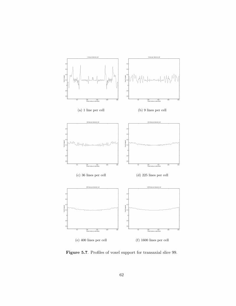
50 100 150 200 250

2.8

2.9

3

3.1

3.2

3.3

3.4

1 line per detector cell

Voxel indices (x direction)

Vox

el s

uppo

rt

(a) 1 line per cell

50 100 150 200 250

2.8

2.9

3

3.1

3.2

3.3

3.4

9 lines per detector cell

Voxel indices (x direction)

Vox

el s

uppo

rt

(b) 9 lines per cell

50 100 150 200 250

2.8

2.9

3

3.1

3.2

3.3

3.4

36 lines per detector cell

Voxel indices (x direction)

Vox

el s

uppo

rt

(c) 36 lines per cell

50 100 150 200 250

2.8

2.9

3

3.1

3.2

3.3

3.4

225 lines per detector cell

Voxel indices (x direction)

Vox

el s

uppo

rt

(d) 225 lines per cell

50 100 150 200 250

2.8

2.9

3

3.1

3.2

3.3

3.4

400 lines per detector cell

Voxel indices (x direction)

Vox

el s

uppo

rt

(e) 400 lines per cell

50 100 150 200 250

2.8

2.9

3

3.1

3.2

3.3

3.4

1600 lines per detector cell

Voxel indices (x direction)

Vox

el s

uppo

rt

(f) 1600 lines per cell

Figure 5.7. Profiles of voxel support for transaxial slice 99.

62

follows

xj = xj ∗µ1600

µtri(5.2)

where xj is the jth voxel, µ1600 is the mean of the voxel support values for the 1600

line intersection model, and µtri is the mean of the voxel support values for the trilin-

ear approach. After normalizing, the standard deviation for transaxial slice 99 of the

trilinear based model was 0.0179. This falls between the standard deviation for the

100 line model, which was 0.0181, and the standard deviation for the 121 line model,

which was 0.0177. Due to the spurious assumption in equation (5.2), namely that the

system model using 1600 lines is the ideal system model, the standard deviation for

the trilinear model cannot be directly compared against the intersection based models.

However, this does show that the standard deviation for the trilinear system model is

in the same neighborhood as using many lines in the intersection based models.

The voxel support values for the central coronal plane of transaxial slice 99 for the

trilinear interpolation model are illustrated in figure 5.8. Note that this profile includes

central dishing similar to the multiline profiles.

5.3 3D Shepp-Logan Phantom Reconstructions

The 3D Shepp-Logan phantom is a well-known analytical phantom consisting of 10

ellipsoids of varying sizes, orientations, and attenuation coefficients used to verify re-

63

50 100 150 200 250

2.8

2.9

3

3.1

3.2

3.3

3.4

Trilinear interpolation

Voxel indices (x direction)

Vox

el s

uppo

rt

Figure 5.8. Trilinear interpolation voxel support.

construction models and algorithms. Although computing a 3D reconstruction for a full

half of the phantom, we will focus on transaxial slice 99, which is shown in figure 5.9.

The 64th iteration of SART, EM, and FWLS using trilinear interpolation and a mul-

tiline model with 144 lines per detector cell are illustrated in figure 5.10. We clamped

the attenuation coefficients of each of these images to the range [0.95, 1.05] before dis-

playing to highlight the internal structures. Furthermore, we normalized the trilinear

interpolation based models by the mean of the ideal phantom, similarly to equation

(5.2).

There are several features worthy of note in these reconstructions. First of all,

none of the reconstruction algorithm and system model combinations faithfully recon-

structed the lower two ellipsoids, although the remaining ellipsoids were accurately

64

Figure 5.9. Original phantom.

(a) Trilinear/SART (b) Trilinear/EM (c) Trilinear/FWLS

(d) Multiline/SART (e) Multiline/EM (f) Multiline/FWLS

Figure 5.10. Phantom reconstructions of transaxial slice 99.

65

reconstructed. There is, however, a noticable change in the attenuation coefficients in

the area of the ellipsoids, which would hopefully draw attention to the area. Secondly,

the EM reconstructions, using both system models, were slightly noisier than the other

reconstructions. This may be due to using the emission derived EM algorithm rather

than a transmission derived algorithm. Thirdly, there is visible ringing in the recon-

structions using multiple lines, although it is not as severe as for the single line model.

Using more lines should gradually improve the reconstructions. Lastly, the outermost

ellipsoid is wider in the reconstructions than in the original. This is more pronounced

when using SART and FWLS. To explain this, we analyze profiles of the reconstructed

images.

In figure 5.11, we plot profiles of coronal slice 114 of the attenuation coefficients of

the reconstructed images against the known values. In the SART and FWLS reconstruc-

tions, the reconstructed values are not tight to the abrupt change in attenuation values

at the edge of the outermost ellipsoid. Thus, when we clamp the attenuation values to

the range [0.95, 1.05], the outermost ellipsoid appears wider than it should. However,

this is more of an artifact associated with the clamping than the reconstruction.

66

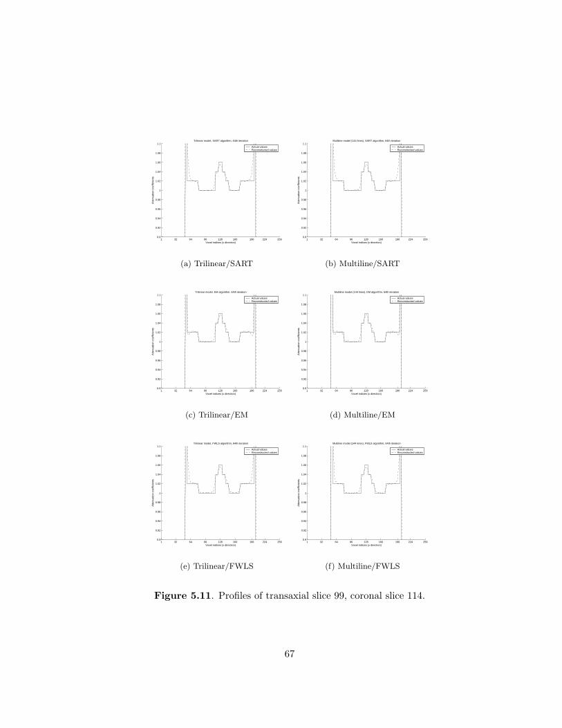
1 32 64 96 128 160 196 224 2560.9

0.92

0.94

0.96

0.98

1

1.02

1.04

1.06

1.08

1.1Trilinear model, SART algorithm, 64th iteration

Voxel indices (x direction)

Atte

nuat

ion

coef

ficie

nts

Actual valuesReconstructed values

(a) Trilinear/SART

1 32 64 96 128 160 196 224 2560.9

0.92

0.94

0.96

0.98

1

1.02

1.04

1.06

1.08

1.1Multiline model (144 lines), SART algorithm, 64th iteration

Voxel indices (x direction)

Atte

nuat

ion

coef

ficie

nts

Actual valuesReconstructed values

(b) Multiline/SART

1 32 64 96 128 160 196 224 2560.9

0.92

0.94

0.96

0.98

1

1.02

1.04

1.06

1.08

1.1Trilinear model, EM algorithm, 64th iteration

Voxel indices (x direction)

Atte

nuat

ion

coef

ficie

nts

Actual valuesReconstructed values

(c) Trilinear/EM

1 32 64 96 128 160 196 224 2560.9

0.92

0.94

0.96

0.98

1

1.02

1.04

1.06

1.08

1.1Multiline model (144 lines), EM algorithm, 64th iteration

Voxel indices (x direction)

Atte

nuat

ion

coef

ficie

nts

Actual valuesReconstructed values

(d) Multiline/EM

1 32 64 96 128 160 196 224 2560.9

0.92

0.94

0.96

0.98

1

1.02

1.04

1.06

1.08

1.1Trilinear model, FWLS algorithm, 64th iteration

Voxel indices (x direction)

Atte

nuat

ion

coef

ficie

nts

Actual valuesReconstructed values

(e) Trilinear/FWLS

1 32 64 96 128 160 196 224 2560.9

0.92

0.94

0.96

0.98

1

1.02

1.04

1.06

1.08

1.1Multiline model (144 lines), FWLS algorithm, 64th iteration

Voxel indices (x direction)

Atte

nuat

ion

coef

ficie

nts

Actual valuesReconstructed values

(f) Multiline/FWLS

Figure 5.11. Profiles of transaxial slice 99, coronal slice 114.

67

5.4 Mouse Data Reconstructions

While the Shepp-Logan phantom is useful as a means of testing reconstruction algo-

rithms and system models, it does not realistically model the process of attenuation

occurring during the aquisition of real data. The phantom projection data is noiseless

and based upon line integrals, which is not physically accurate. Thus, we also tested

the framework using X-ray CT data collected from a mouse scan using the MicroCAT

scanner.

The projection data has dimensions 512×1022. We reconstructed half of the volume

at 256 × 256 resolution per transaxial slice, so the voxel space has dimensions 256 ×

256×512. We ran each algorithm to 64 iterations using the same algorithms and system

models as in the previous section. Some results are shown in figures 5.12 and 5.13 for

transaxial slices 350 and 450, respectively. Since the system matrix grew too large to

store in main memory during the mouse reconstructions, the system matrix was stored

on disk and read incrementally.

The attenuation coefficients of the EM produced images were clamped to the same

range as the SART produced images to facilitate visual comparison. Otherwise, the

EM images would be slightly darker than the SART and FWLS images after conversion

to gray level values. Unfortunately, there is no known set of correct images to com-

pare against these reconstructions. However, the reconstructions demonstate that the

framework is capable of handling real world CT data.

68

(a) Trilinear/SART (b) Multiline/SART

(c) Trilinear/EM (d) Multiline/EM

(e) Trilinear/FWLS (f) Multiline/FWLS

Figure 5.12. Mouse reconstuctions (transaxial slice 350).

69

(a) Trilinear/SART (b) Multiline/SART

(c) Trilinear/EM (d) Multiline/EM

(e) Trilinear/FWLS (f) Multiline/FWLS

Figure 5.13. Mouse reconstuctions (transaxial slice 450).

70

Table 5.1

System matrix storage requirements.

Trilinear Interpolation Multiline Intersection

Phantom Data

Number of elements stored 1, 011, 298, 717 812, 056, 052

Approximate storage (bytes) ≈ 8GB ≈ 6.5GB

Mouse Data

Number of elements stored 13, 430, 851, 808 8, 662, 072, 989

Approximate storage (bytes) ≈ 107.5GB ≈ 70GB

5.5 Storage Analysis

As noted previously, each of the 23 nodes used for the reconstruction has 2GB of RAM.

Thus, the size of the system matrix is bound above by 46GB for storage in main memory.

Note that in reality the limit is lower than this due to the overhead of other storage.

For the Shepp-Logan phantom reconstructions, the matrix is small enough to store

in main memory. However, for the mouse data reconstructions, the matrix must be

stored on disk. The total number of elements and approximate memory requirements

for the phantom and mouse reconstructions are given in table 5.1. The multiple line

model used 144 lines per detector cell. Note that the values in the table correspond to

the number of elements stored, not the total number of elements in the system matrix.

Due to symmetries, the total number of system matrix elements is approximately eight

times that of the number of elements stored.

One additional interesting statistic involving the number of system matrix elements

is the distribution of these elements among the cluster nodes. This is plotted in figure

5.14 for the trilinear interpolation system model used for the mouse reconstruction.

71

0 1 2 3 4 5 6 7 8 9 10 11 12 13 14 15 16 17 18 19 20 21 225.55

5.6

5.65

5.7

5.75

5.8

5.85

5.9

5.95

6

6.05x 10

8 Distribution of system matrix elements across cluster nodes

Cluster node

Num

ber

of e

lem

ents

Figure 5.14. Distribution of system matrix across cluster nodes.

Ideally, this distribution would be almost uniform. However, in this case, the higher

numbered nodes have more matrix elements than the lowered numbered nodes. This is a

result of distributing the data based on projections. As the view angle increases toward

45◦, the number of intersections of the projection rays with the voxel space increases

due to the increase in the total intersection length of the projection rays with the voxel

space. In this example, the node with the most data manages approximately 7% more

data than the node with the least amount of data. Modest performance gains may be

achieved by distributing the data more uniformly, but that is not explored in this thesis.

72

5.6 Performance Analysis

We performed an analysis of the performance of system model construction and the it-

erations of the EM algorithm. We further subdivide the iterative phase by the projector

operations and MPI communication. The EM algorithm includes one forward and back-

projector per iteration, plus an extra initial backprojection for scaling purposes. This

is typical of the iterative algorithms and can thus be used to gauge the performance of

the iterative framework.

5.6.1 System Model Analysis

In order to evaluate the performance of the system model construction, we ran sev-

eral experiments using the same scanner configuration as for the Shepp-Logan phantom

above. Recall that this includes a 256 × 256 detector and that each MPI node is re-

sponsible for calculating system model data for two projections. Thus, each node must

calculate line intersection data for 131, 072 projection rays in the single line and trilinear

interpolation models. For multiple line models, this number scales with the number of

lines per detector cell.

Recall that with the multiple line intersection based models, the values stored in

the system matrix are the averages of the intersection lengths of each of the lines with

a given voxel. Thus, in addition to the line intersection computation code, there must

be row averaging code to compute the final row to be stored in the system matrix.

The total system matrix computation time is the sum of the intersection computation

73

1 4 9 16 25 36 49 64 810

100

200

300

400

500

600

700

800

Number of lines per detector cell

Tim

e (s

ecs)

Line intersection based system model computation timings

Intersection ComputationRow AveragingTotal

Figure 5.15. Line intersection based system model computation timings.

time and the row averaging time. These times are plotted in figure 5.15 for increasing

numbers of lines per detector cell. The times plotted were recorded from node 22. As

shown in figure 5.14, this node computes the most data and will subsequently have the

longest run times.

Note that the line intersection computation scales almost perfectly linearly, with the

row averaging curve slightly below. The result is that the system matrix computation

time for the line intersection based models scales very well.

The trilinear interpolation model took 90 seconds to compute with the same ge-

ometry as above. This places the trilinear interpolation model between the 9 and 16

multiple line models in terms of computational cost.

The system model calculation currently only uses a single processor per node. Since

74

the cluster nodes each have two processors, performance gains could be achieved by

distributing the system matrix calculation between the two processors.

5.6.2 Iteration Analysis

Each iteration of the typical iterative reconstruction algorithms includes a single for-

ward and backprojection as well as one MPI communication following the backprojec-

tion. The EM algorithm matches this behavior and was thus chosen as a representative

algorithm for performance analysis. Note that the EM algorithm also includes a single

backprojection before the first iteration for scaling purposes.

Since the size of the system matrix for the Shepp-Logan phantom reconstructions

is relatively small, we store the matrix in main memory. Thus, the computation in the

projectors consists of recovering the matrix from the symmetries and performing the

necessary multiplications. The other major cost per iteration is the MPI communication.

To measure the performance of these operations, we ran the EM algorithm on the Shepp-

Logan phantom data using the trilinear interpolation model for 32 iterations. To get

approximate relative costs, we averaged the timings for each projector and the MPI

communication across all nodes. The resulting approximate cost per iteration is shown

in figure 5.16.

As the system matrix size increases, it must be stored to disk rather than in main

memory. The need to read the system matrix from disk on demand will significantly

increase the time spent in the projectors. Since the system matrix for the mouse recon-

structions was large enough to require disk storage, we use it to gauge the performance

75

9 sec

9 sec

7 sec

2 sec

Approximate cost distribution per iteration with system matrix in main memory

Forward Projector

Back Projector

MPI Communication

Other

Figure 5.16. Cost distribution per iteration (main memory).

impact of disk storage. For this experiment, we ran the EM algorithm on the mouse

data using the trilinear interpolation model for 4 iterations. We again averaged the

costs per iteration. The results are shown in figure 5.17. Recall from table 5.1 that the

system matrix for the mouse reconstruction was approximately 13 times larger than for

the Shepp-Logan phantom. Thus, if the system matrix were stored in main memory,

we would expect the cost per iteration of each projector to increase by a factor of about

13. It in fact increases by a factor of almost 24, so the disk access nearly doubles the

cost of the projectors in this case.

5.6.3 Overall Performance

The total run time for 32 iterations of the Shepp-Logan phantom data using the trilinear

interpolation model was approximately 16.5 minutes. With an average iteration time

76

219 sec

90 sec

8 sec

Approximate cost distribution per iteration with system matrix on disk

Back Projector

Forward Projector

205 sec

MPI Communication

Other

Figure 5.17. Cost distribution per iteration (disk storage).

of 27 seconds and a system model computation time of 90 seconds, this leaves just over

half a minute for overhead related to reading the projection data, calculating the scaling

factors, and other setup procedures. Note that if this same system model was used, but

the system matrix was recomputed rather than stored, the average iteration time would

be at least 180 seconds since the matrix is needed twice per iteration.

The total run time for 4 iterations of the mouse data using the trilinear interpolation

model was approximately 42.5 minutes. The average iteration time was just over 8.5

minutes. Thus, the overhead in this case was nearly 8.5 minutes. The increase in over-

head is due to the larger projection data set and the costly scaling factor computation,

which is accomplished with a backprojection. In addition to the 42.5 minute reconstruc-

tion, the system model generation took about 13.5 minutes, although this cost can be

absorbed before performing the reconstruction. Computing the same system matrix on

77

the fly would therefore slow the iterations to at least 27 minutes. Thus, even with the

cost associated with disk storage, the per iteration cost is much lower in this case than

if we recomputed the matrix on demand. If a simple enough system model is chosen,

the on the fly computation may perform better than disk storage, but the model would

likely yield inferior reconstruction results.

78

Chapter 6

Conclusions and Future Work

In this work, we accomplished the overall goal of building a framework to support

high-resolution iterative CT data reconstructions. The reconstructions of the mouse

CT data exhibit that the framework is capable of managing problems of significant size.

However, the storage and computational requirements are likely still too high for clinical

deployment. As computer technology progresses, the requirements will become easier

to satisfy.

Of the system models analyzed, trilinear interpolation seems to be the most promis-

ing. While the storage requirements are higher than for the line intersection based

models, the computational advantage over using an adequate number of lines is signif-

icant. We could also lower the computational and storage requirements by decreasing

the ∆s value used for the interpolation, although that would require re-analyzing the

system model with respect to accuracy. Furthermore, we observed no undesirable ef-

79

fects in regards to the trilinear interpolation model during this work. However, a more

rigorous analysis of the smoothing effects of this model are in order.

Since analyzing various algorithms was not a goal of this thesis, little work was per-

formed in this regard. However, now that the framework has been developed, there are

many possibilities for future work, including comparative analysis of various algorithms.

One possible area of future work involves improving the current system models as

well as developing and analyzing new system models. As noted in chapter 2, each of

the current system models includes central dishing in the voxel support values. Com-

pensating for this dishing may increase the quality of the generated system matrices.

Furthermore, researching possible methods for calculating the ideal system matrix based

on volumetric intersections is another possibility for future research. Even if the compu-

tational cost is high, an ideal system model would be useful for comparative purposes.

In addition to continued system model research, the set of available algorithms can

be expanded and more rigorous analyses performed. For example, penalties can be

included in most iterative algorithms for regularization purposes. Moreover, additional

algorithms can be added to the framework. For example, work has been performed

by Nuyts et al. to derive solutions to the transmission EM algorithm using regular

forward and backprojectors [9]. It would be interesting to compare this algorithm to

the EM algorithm implemented in this thesis. Furthermore, we could perform a more

rigorous comparison of algorithms using a real data phantom as opposed to the analytical

Shepp-Logan phantom. A comparative analysis of the iterative algorithms to FBP is

80

also warranted.

Finally, there are several areas of further research with regards to the current imple-

mentation. As noted in section 5.5, the current load distribution is not ideal. Further

equalizing the distribution would increase performance. Also, the inclusion of check-

pointing support would be beneficial. Currently, if the program terminates unexpect-

edly, it cannot restart at the point of failure. The generated data is available, but all

of the work must be repeated to perform additional iterations. It should be possible to

save the voxel space data and use it to bootstrap the iterative algorithms.

The development of the iterative framework enables further research into any of

these areas.

81

Bibliography

82

Bibliography

[1] R. Barrett, M. Berry, T. F. Chan, J. Demmel, J. Donato, J. J. Dongarra, V. Ei-

jkhout, R. Pozo, C. Romine, and H. van der Vorst. Templates: Building Blocks for

Iterative Methods. SIAM, Philadelphia, PA, 1993.

[2] I. A. Elbakri and J. A. Fessler. Statistical image reconstruction for polyenergetic

x-ray computed tomography. IEEE Trans. on Med. Imag., 21(2):89–99, February

2002.

[3] L. A. Feldkamp, L. C. Davis, and J. W. Kress. Practical cone-beam algorithm. J.

Opt. Soc. Amer., 1:612–619, 1984.

[4] S.S. Gleason, H. Sari-Sarraf, M. J. Paulus, D.K. Johnson, S.J. Norton, and M. A.

Abidi. Reconstruction of multi-energy x-ray computed tomography images of lab-

oratory mice. IEEE Transactions on Nuclear Science, 46(4):1081–1086, August

1999.

[5] F. Jacobs, E. Sundermann, B. De Sutter, M. Christiaens, and I. Lemahieu. A fast

algorithm to calculate the exact radiological path through a pixel or voxel space.

83

[6] A. C. Kak and M. Slaney. Principles of Computerized Tomographic Imaging. So-

ciety of Industrial and Applied Mathematics, 2001.

[7] K. Lange and R. Carson. Em reconstruction algorithms for emission and transmis-

sion tomography. Journal of Computer Assisted Tomography, 8(2):306–316, April

1984.

[8] L. B. Lucy. An iterative technique for the rectification of observed distributions.

The astronomical journal, 79(6):745–754, June 1974.

[9] J. Nuyts, B. De Man, P. Dupont, M. Defrise, P. Suetens, and L. Mortelmans. Iter-

ative reconstruction for helical ct: a simulation study. Phys. Med. Biol., 43(4):729–

737, 1998.

[10] M. J. Paulus, H. Sari-Sarraf, S. S. Gleason, M. Bobrek, J. S. Hicks, D. K. Johnson,

J. K. Behel, L. H. Thompson, and W. C. Allen. A new x-ray computed tomography

system for laboratory mouse imaging. IEEE Transactions on Nuclear Science,

46(3):558–564, June 1999.

[11] W. H. Richardson. Bayesian-based iterative method of image restoration. Journal

of the Optical Society of America, 62(1):55–59, January 1972.

[12] L. A. Shepp and Y. Vardi. Maximum likelihood reconstruction for emission tomog-

raphy. IEEE Trans. on Med. Imag., MI-1(2):113–122, October 1982.

[13] R. L. Siddon. Fast calculation of the exact radiological path for a three-dimensional

ct array. Medical Physics, 12(2):252–255, 1985.

84

[14] G. Wang, C. R. Crawford, and W. A. Kalender. Multirow detector and cone-beam

spiral/helical ct. IEEE Trans. on Med. Imag., 19(9):817–821, Sept. 2000.

[15] G. Wang, D. L. Snyder, J. A. O’Sullivan, and M. W. Vannier. Iterative deblurring

for ct metal artifact reduction. IEEE Trans. on Med. Imag., 15(5):657–663, October

1996.

[16] G. L. Zeng and G. T. Gullberg. A study of reconstruction artifacts in cone beam

tomography using filtered backprojection and iterative em algorithms. IEEE Trans.

on Nucl. Sci., 37(2):759–767, 1990.

[17] G. L. Zeng and G. T. Gullberg. Unmatched projector/backprojector pairs in an

iterative reconstruction algorithm. IEEE Trans. on Med. Imag., 19(5):548–555,

2000.

85

Vita

Thomas Matthew Benson was born in Greeneville, TN. He attended grade school

and high school there and received a high school diploma from Greeneville High School

in 1997. He subsequently attended the University of Tennessee, Knoxville, where he

completed Bachelor of Science degrees with highest honors in Computer Science and

Mathematics in May 2001. He is continuing his work at the university toward a doctorate

in Computer Science.

86