IS THERE A CONTINENTAL BIAS IN TRADE?

Salvador Gil-Pareja*

Rafael Llorca-Vivero

José Antonio Martínez-Serrano

University of Valencia

January 17th, 2010

Abstract

Geography is an important determinant of bilateral trade volumes. This paper investigates the potential existence of a continental bias in world trade flows on a sample of 182 countries over the period 1990-2006. Using traditional estimation techniques and recent developments in the econometric analysis of the gravity equation, we find robust evidence of an economically significant continental bias in trade. Further, a continent-by-continent analysis reveals that Oceania, America, Europe and Asia are behind this result, whereas for Africa the results are not conclusive.

Key words: Continental bias, gravity equation, intercontinental and intra-continental

trade costs.

JEL Classification numbers: F14.

*Corresponding author: Salvador Gil Pareja, Facultad de Economía, Departamento de Estructura

Económica, Av. de los Naranjos s/n, C.P. 46022, Valencia, Spain. Email: Salvador.Gil-Pareja@uv.es;

Tel. 34963828349. Fax 34963828354. We are extremely grateful to Marc Melitz for invaluable help with

the implementation of the Helpman, Melitz and Rubinstein (2008) estimator. We also thank Silviano

Esteve for valuable comments. This study is part of a research project financed by Ministerio de Ciencia y

Tecnología (projects SEJ2006-07238/ECO and ECO2009-08181) and has been part-founded by the

European Regional Development Fund (ERDF). We also thanks financial support from the Generalitat

Valenciana (GVPROMETEO2009-098). A previous version of this article was published as Working

Paper No 440/2009 of FUNCAS.

1. Introduction

Continental boundaries matter for policy makers. While no continental-wide

trade agreement is into force, the creation of transcontinental free trade agreements has

long been an ideal. Since the early 1960s, by the establishment of the Organization of

African Unity, African countries where encouraged to combine their economies into

sub-regional markets that would ultimately form an African-wide economic union. This

goal was translated into concrete form with the signature of the African Economic

Community Treaty (into force since May 1994), which establishes a 6 stage process

over 34 years ending with a continent-wide economic and monetary union (and thus

also a free trade area within this continent). In the Americas, the first specific plan for a

hemisphere-wide trade agreement goes back to the First International Conference of the

American States in 1889. The most recent attempt is the Free Trade Area of the

Americas (ongoing since 1994) that would create a continental-wide free trade

agreement including all democracies in the Western Hemisphere.1 The dream of the

European integration started six decades ago. Since then, the number of countries

participating in the European Union (EU) has increased from 6 in the 1950s to 27 in

2007. Additionally, countries like Turkey, Croatia and Macedonia have gained

candidate status whereas other European countries like Albania, Serbia and Montenegro

formally have applied for membership in the EU.2 Moreover, the European Economic

Area (into force since 1994) has created a free trade agreement between remaining

European Free Trade Association (EFTA) members (except Switzerland) and the EU. In

Asia, the major countries in the region are rigorously pursuing preferential trade

1 Nowadays, the successful conclusion of the negotiations among the 34 democracies participating in the

Americas process remains in doubt. 2 According to Article 49 of the Maastricht Treaty any European state that respects the principles of

liberty, democracy, respect to human rights and fundamental freedoms may apply to join the EU.

1

agreements, which may eventually lead to an Asian-wide trade bloc.3 In fact, there is

currently intense debate in Asian policy circles about the impact of the process of Pan-

Asian integration on insiders and outsiders (Francois et al, 2009). Finally, in Oceania,

business communities have proposed to extend the Australia-New Zealand Closer

Economic Relations Trade Agreement to other Pacific Island nations.

The relationship between geography and trade has long been a central topic in

international economics. Since the first application of the gravity equation to

international trade in the early 1960s (Tinbergen, 1962), a vast empirical literature has

documented the importance of geographical variables as determinants of bilateral trade

flows. In addition to the geographical distance (one of the two basic variables of the

gravity models that serves to reflect transportation costs), other variables, such as

adjacency (common land border), remoteness of countries, insularity, or the landlocked

status of trading partners has been used to capture geographical factors influencing trade

costs. An important geographical factor that may have an effect on international trade,

and that has not properly been considered by the empirical literature, is the location of

countries within the same continent. 4 The goal of this paper is to investigate the

possible existence of a continental bias in trade based on differences in trade costs

between and within continents.5

3 The ASEAN-China agreement of November of 2004, the ASEAN-India Trade in Goods Agreement (in

force since January of 2010) and the more ambitious proposals of China-India and the ASEAN+3

(ASEAN plus China, Japan and South Korea) are examples to the trend towards regionalism in Asia. 4 Frankel, Stein and Wei (1993) also draw the boundaries at continental bloc level, but they do not

consider all the countries in each continent. In their paper the continents are The Americas (including

only 13 countries), the European Community (11 countries) and East Asia (10 countries). 5Our paper is related to another strand of the empirical gravity literature: the so-called border effect (home

bias) literature, which documents that political borders contribute significantly to overall trade costs

strongly diminishing inter- versus intra-national shipments. See, in addition to the seminal work by

McCallum (1995), Helliwell (1996, 1997, 1998), Wei (1996), Anderson and Smith (1999a, 1999b),

2

The existence of differences in trade costs between continents and within them

has been considered by the economic geography literature in the context of the

theoretical welfare analysis of preferential trade agreements (PTAs). In particular, the

relationship between intra-continental and intercontinental trade costs is a crucial

element of the hypothesis of "natural" trading partners with clear theoretical welfare

implications.6 With zero intercontinental transport costs, PTAs along continental lines

decrease welfare (Krugman, 1991a). With prohibitive intercontinental transport costs,

such agreements increase welfare (Krugman, 1991b). However, in the intermediate

realistic case where intercontinental transportation costs are neither zero nor prohibitive

(but greater than transportation costs within continents) the relationship between

intercontinental and intra-continental transportation costs determines the net impact of

PTAs on welfare (Frankel, Stein and Wei, 1993, 1995 and 1996).

According to the hypothesis of natural trading partners, in order to limit the risk

of trade diversion and the associated loss of welfare, trade blocs should be formed

including countries that already traded disproportionately more in the absence of a

preferential trade agreement. If there is a positive continental bias in trade, that is, if

ceteris paribus countries located within the same continent trade more with each other

than with countries located in other continents, countries inside a continent can be

considered “natural” trading partners and, therefore, preferential trade agreements

among them are more likely to be welfare-improving.7 On the contrary, the evidence of

Nitsch (2000), Head and Mayer (2000), Hillberry (2002), Anderson and van Wincoop (2003), Evans

(2003), Chen (2004), Gil et al (2005), or Gil, Llorca and Martínez-Serrano (2006), among others, 6 The literature on the economic determinants of the formation of PTAs also explicitly considers

intercontinental and intra-continental transportation costs among multiple countries on multiple

continents (see, for example, Baier and Bergstrand, 2004 and Egger and Larch, 2008). 7 The term natural trading partner goes beyond pure distance arguments and, therefore, by transport costs

we refer to any kind of trade costs.

3

a negative continental bias in trade would suggest that continental preferential

agreements may be welfare decreasing. Continental trading blocs that reduce welfare

are called "super-natural".8

In particular, this paper aims at answering two main questions. First, all other

things equal, countries within the same continent trade more with each other than

countries located on different continents? Second, are there differences in the size and

sign of the continental bias across continents? In addition to the academic interest of

these questions, they are especially important for policy reasons. During the last two

decades there has been a dramatic rise in the number of economic integration

agreements all over the world. Most of these trade and monetary agreements are

continental blocs, i.e. blocs formed by two or more countries within the same

continent.9 Moreover, as mentioned above, there are well documented initiatives to

create continental-wide free trade agreements. The analysis in this paper may shed some

lights about the convenience of such sort of agreements. In particular, the existence of a

positive continental bias in trade would both give support to the implementation of

regional trading blocs along continental lines, and provide arguments in favour of

transcontinental projects.

In order to explore continental bias in trade we estimate gravity equations using

both traditional estimation techniques and two recently developed econometric

approaches: the fixed effects vector decomposition technique suggested by Plümper and

Troeger (2007) and the two-stage estimation procedure proposed by Helpman, Melitz

8 Frankel Stein and Wei (1993, 1995 and 1996) set up a trade theory model of many countries that are

grouped into continents with high trade costs across continents and low costs within them. According to

these authors the term "super-natural" refers to a continental PTA that is welfare-reducing on net due to

relatively low intercontinental transportation costs. 9 Notwithstanding, it is worth noting that an important trend in international economic integration in

recent years is the proliferation of intercontinental trade agreements.

4

and Rubinstein (2008). The first technique allows the estimation of the coefficient of

interest controlling for time-invariant omitted bilateral variables. The second framework

allows to correct for selection bias and to account for exporter heterogeneity. The

sample covers 182 countries over the period 1990-2006. To preview our results, we find

robust evidence of a positive continental bias in trade. The analysis by continents

reveals that Oceania, America, Europe and Asia are behind this finding. The results for

Africa are not conclusive.

The paper is structured as follows. Section 2 presents the methodology. Section

3 describes the data. Section 4 discusses the estimation results. Finally, section 5

concludes the paper.

2. Methodology

The gravity equation of trade is considered to be one of the most successful

empirical frameworks in international economics. It relates bilateral trade flows to

economic size (GDP), distance and other factors that affect trade barriers.10 In particular,

the literature on the border effect has made use of the gravity equation to estimate the

size of the home bias in trade. In this paper, we also use that methodology to assess the

existence and magnitude of the continental bias.

The typical gravity equation estimated in the border effect literature can be

written as follows for any given time period:

0 1 2 3 4ln ln ln lnij i j ij ij

ij

Trade GDP GDP Dist HomeOthercontrols uβ β β β β= + + + +

+ + (1)

10 Initially the gravity model lacked theoretical foundation. However, since the end of the 1970´s the

situation has changed and nowadays the gravity model is backed up by sound theory. See, among others,

Anderson (1979), Bergstrand (1985 and 1989), Deardoff (1998), Evenett and Keller (2002), Anderson

and van Wincoop (2003) and Helpman, Melitz and Rubinstein (2008).

5

where Tradeij is the bilateral trade flow between i to j, GDPi and GDPj are the gross

domestic products, Distij denotes the distance between i and j, Homeij is a dummy

variable that takes the value of one for trade flows within countries and zero otherwise,

and Othercontrols are a set of variables that are included to capture variation in various

trade costs, such as binary variables for the presence of a land border, a common

language or being a member of the same trade agreement. In this set-up, the border

effect is measured by the estimated coefficient of the dummy variable Home.

Despite being used in many studies on the border effect, equation (1) is likely to

be mis-specified owing to ignoring theoretical foundations for the gravity equation. As

Anderson and van Wincoop (2003) emphasize (in the context of the border effect

literature) the gravity model theory implies that the researcher must take into account

the role of relative prices ("multilateral resistance", in Anderson and van Wincoop’s

terminology).11 The usual solution to the presence of such multilateral resistance is to

include country fixed effects (CFE) for both the exporter and the importer countries

when estimating gravity equations. However, following Anderson and van Wincoop

(2004), in a panel framework, separate country fixed effects should be included for each

year as multilateral resistance may change over time. The specialised literature refers to

these estimates as country year fixed effects (CYFE).12

Time-varying country dummies should completely eliminate the bias stemming

from the omission of multilateral resistance terms, but CYFE do not eliminate all kinds

11 While the methodological contribution of Anderson and van Wincoop (2003) is made trying to provide

a "solution" to the border puzzle, it is indeed important for the proper estimation of gravity equations in

other applications of the international trade literature. 12 Following Anderson and van Wincoop (2004) and Feenstra (2004), several recent studies include

country year fixed effects in the estimation of gravity equations for international trade flows. See, among

others, Klein and Shambaugh (2006), Baier and Bergstrand (2007) or Gil, Llorca and Martínez- Serrano

(2008a).

6

of omitted variable bias (Baldwin and Taglioni, 2006). Time-invariant omitted variables

that affect bilateral trade may still bias the estimates. In other words, time-varying

country dummies do not remove the bias stemming from the correlation between the

determinants of bilateral trade that have been included and the determinants that are

unobservable to the researcher. Recognizing this, Baldwin and Taglioni (2006), Baier

and Bergstrand (2007), Gil, Llorca and Martínez-Serrano (2008b, 2008c) and Eicher

and Henn (2009) argue in favour of using time-invariant pair dummies in addition to

time-varying country dummies. The problem with this estimation is that until recently

there was not a satisfactory way for estimating time-invariant variables once country-

pair fixed effects (CPFE) are included in the regression.13 However, nowadays it is

possible to consider the estimation of time-invariant variables accounting for

unobserved bilateral heterogeneity by the use of the fixed effects vector decomposition

technique suggested by Plümper and Troeger (2007).

More recently, Helpman, Melitz and Rubinstein (2008) (henceforth HMR) have

developed a theoretical model that generalizes the Anderson and van Wincoop (2003)

framework in two ways. Firstly, they account for non-observable firm heterogeneity and

fixed trade costs in line with the so-called new-new trade theory (Melitz, 2003).

Secondly, they account for asymmetries in the volume of bilateral exports between

countries depending on the direction of export flows (from i to j versus from j to i).

Moreover, they also develop the empirical framework for estimating the gravity

equation derived in their model.

13 The conventional fixed effect “within” estimator in panel data does not allow the estimation of the

coefficients of bilateral time-invariant variables. Hausman and Taylor (1981) developed a method of

instrumental variables that solves this problem. However, as Plümper and Troeger (2007) point out, the

Hausmann-Taylor procedure, in addition to have poor small sample properties, leaves researchers with a

discretionary choice about which variables are endogenous that largely influence the results.

7

In this paper we estimate for the first time the potential existence of a

continental bias in trade. To this end, we estimate the following general equation:

0 1 2 3 4

5 6 7 8

9 10 11 12

13 14 15

ln ln ln lnijt it jt ij ij

ij ij ij ij

ij ij it jt

ijt ijt ij ijt

X GDP GDP Dist Contiguity

Island Landlooked Language Colony

ComCountry Creligion PR PR

CU PTA SameCont u

β β β β β

β β β β

β β β β

β β β

= + + + +

+ + + +

+ + + +

+ + + + (2)

where i and j denote trading partners, t is time, and the variables are defined as follows:

Xijt are the bilateral export flows from i to j14,

GDP denotes Gross Domestic Product,

Dist denotes the distance between i and j,

Contiguity is a dummy variable equal to one when i and j share a land border,

Island is the number of island nations in the pair (0, 1, or 2),

Landlocked is the number of landlocked areas in the country-pair (0, 1, or 2),

Language is a dummy variable which is unity if i and j have a common language,

Colony is a binary variable which is unity if i ever colonized j or vice versa,

ComCountry is a binary variable which is unity if i and j were part of a same county in

the past,

Creligion is an index of common religion (% Protestants in country i * % Protestants in

country j) + (% Catholics in country i * % Catholics in country j) + (%Muslims in

Country i * % Muslims in country j),

PR is an index of political rights on a 1 to 7 scale,

CU is a binary variable which is unity if i and j use the same currency at time t,

14 Many authors treat the average of two-way bilateral trade as the dependent variable. However, all

theories that underlie a gravity-like specification yield predictions on unidirectional bilateral trade rather

than two-way bilateral trade. In this paper, we use unidirectional trade data. Hence, our specification is

more closely grounded in theory.

8

PTA is a binary variable which is unity if i and j belong to the same preferential trade

agreement,

SameCont is a dummy variable that takes the value of one for country pairs located

within the same continent and zero otherwise, and

uijt is the standard classical error term.

The coefficient of interest to us is β15. If the trading relations between countries

within the same continent are stronger than those between countries located on different

continents, then the estimated coefficient of SameCont would be positive and

statistically significant.

We follow the norm in the border effect literature and we will begin by

estimating the gravity equation (2) using conventional ordinary least squares (with a full

set of year-specific intercepts added). Next we will run the gravity equation using both

CFE and CYFE. The strategy of using CFE sufficiently addresses multilateral resistance

in a cross section but, as noted before, CYFE are required to comprehensively control

for multilateral resistance in panel datasets. However, a part of the force of the paper

rests in employing two additional and recently developed econometric approaches: the

fixed effects vector decomposition technique suggested by Plümper and Troeger (2007),

which allows us to estimate the coefficient of interest controlling for time-invariant

omitted bilateral variables, and the two-stage estimation procedure proposed by HMR

(2008), which allows us to correct for selection bias and to account for exporter

heterogeneity. None of them have been considered by the border effect literature. Both

procedures are briefly outlined next.

The fixed effect vector decomposition technique proposed by Plümper and

Troeger (2007) consists of three stages. In a first stage they obtain the unit fixed effects

vector (country-pair fixed effects in the context of this paper) by estimating a fixed

9

effect model that excludes the (bilateral in our case) time-invariant variables. In a

second stage, the fixed effects vector is decomposed into a part explained by the

(bilateral) time-invariant variables and an error-term. Finally, in the third stage, this

error-term accounts for the unobserved (bilateral) fixed effects and, thus, captures the

potential of omitted variable bias.

The HMR (2008) estimation procedure consists in two-stages. In the first stage

they estimate a probit equation that specifies the probability that country i exports to j

conditional on the observable variables. In the second stage, predicted components of

this equation are used to estimate the gravity equation. This procedure simultaneously

corrects for two types of potential biases: a Heckman selection bias and a bias from

potential asymmetries in the trade flows between pairs of countries.

More formally, in a first stage they estimate a probit equation of the type:

Pr ( 1/ var ) ( , , , , )ij i j ij ij ijob T observed iables X Zχ λ= = Φ ε (3)

where Tij is an indicator variable equal to 1 when country i exports to j and zero

when it does not, Φ is the cumulative distribution function of the standard normal

distribution, iχ and jλ are exporter and importer fixed effects, Xij are variables which

affect both the probability and the volume of trade, and Z ij represents variables that are

used for the exclusion restriction, that is, those that affect the probability of observing a

positive volume of trade but do not impact the volume of trade if this were to be

positive.15 Using the probit regression, they construct two variables that are included as

regressors in the second stage estimation. One is the inverse of Mills ratio and the other

is an expression that controls for firm size heterogeneity. In particular, the second stage

15 In this set-up, parameter identification requires the existence of a variable that affects the probability of

observing a non-zero flow between two countries but not the volume. Alternatively, a variable which

affects both decisions in opposite directions would also work.

10

consists in the estimation for a given year of the following non-linear equation for all

country-pairs with positive trade flows:

{ }* **

0ln ln exp ( ) 1ijij j i ij ijij ijTrade X zβ λ χ γ θη δ η ε⎡ ⎤= + + − + + + − +⎢ ⎥⎣ ⎦$

(4)

where *

ijη is the inverse Mills ratio and * 1( )ij ijz ρ−= Φ$ in which ijρ are the

estimates from the probit equation.16

3. Data

The trade data for the dependent variable (export flows from country i to country

j) come from the “Direction of Trade” (DoT) dataset built up by the International

Monetary Fund (IMF). The data comprise bilateral merchandise trade between 182

countries and territories (see Table A1) over the period 1990-2006. 17 The DoT dataset

provides FOB exports in US dollars. These series are converted into constant terms

using the American GDP deflator taken from the Bureau of Economic Analysis (US

Department of Commerce).

The independent variables come from different sources. GDP data in constant

US dollars are taken from the World Development Indicators (World Bank). For

location of countries (geographical coordinates), used to calculate Great Circle

Distances, and the construction of the dummy variables for physically contiguous

neighbours, island and landlocked status, common language, colonial ties, common

religion and common country background data are taken from the CIA's World

Factbook. Data on political rights come from Freedom in the World Comparative and 16 Since equation (3) is non-linear in δ, following HMR (2008) we estimate it using maximum likelihood. 17 It is noteworthy that not all the areas considered are countries in the conventional sense of the word.

We also include some dependencies, territories and overseas departments in the data.

11

Hisorical Data, 2009. The indicators of preferential trade agreements have been built

using data from the World Trade Organization, the Preferential Trade Agreements

Database (The Faculty of Law at McGill University) and the web site

http://ec.europa.eu/trade/issues/bilateral/index_en.htm. The indicators of currency

unions are taken from Reinhart and Rogoff (2002), CIA's World Factbook and Masson

and Pattillo (2005). The sample includes 192 preferential trade agreements (plurilateral

and bilateral) and 17 currency unions.18

4. Empirical results

We begin by estimating the possible existence of continental bias in trade using

some traditional estimation techniques: OLS, CFE and CYFE. Traditional estimates of

the gravity equation use data on country pairs with positive volumes of trade. The

results are reported in Table 1. Columns 1 to 3 present the results using pooled OLS

including year dummies. The gravity equation is run first without taking into account

the existence of economic integration agreements in order to check how the estimated

coefficient of the variable of interest is affected by this fact (column 1). The gravity

equation works well. The estimated coefficients are, in general, economically and

statistically significant with sensible interpretations. The negative effect of a common

religion is the only exception. Economically larger countries trade more and more

distant countries trade less. Landlocked countries trade less, whereas sharing a common

border or a common language increase trade. The existence of colonial ties encourages

18 The list of preferential trade agreements considered appears in Appendix B (Tables B1 and B2). The

expression PTAs in this paper refers also to other agreements involving a higher degree of economic

integration. In fact, most economic integration agreements considered in the sample are free trade

agreements. The list of currency unions appears in Table B3.

12

trade, as do being islands or part of the same country in the past. Finally, political rights

also affect positively trade.19

In the gravity equation framework, if there was nothing to the notion of

continental bias, then a dummy variable capturing whether two countries are both

located on the same continent ought not to be statistically significant. However, as we

show in this paper, this is not the case. In column 1, the estimated coefficient of the

variable of interest is positive (0.358) and statistically significant at conventional levels

suggesting that being on the same continent raises bilateral trade.

Since the early 1990s there has been a proliferation of economic integration

agreements all over the world. An important feature of this wave of economic

integration among countries is that most trade and monetary agreements has been

created along continental lines.20 Therefore, one may think that trade policy is likely

behind the existence of a border effect at the continental level. In order to check if it is

the case, in column 2 we control for the existence of PTAs and currency unions (CUs)

around the world including two additional dummy variables: one for PTAs and the other

for CUs. The estimated coefficients of both variables are positive (countries belonging

to the same PTA trade more as do countries sharing a common currency), highly

statistically significant and in line with estimates from the literature. Moreover, the

inclusion of these variables in the equation reduces the magnitude of the coefficient of

19 Political Rights are measured on a one-to-seven scale, with one representing the higher degree of

freedom and seven the lowest. Therefore, according to the definition of this variable a greater value of

this variable implies less political rights. 20 The European Union (EU), the North America Free Trade Agreement (NAFTA), the Southern Cone

Common Market (MERCOSUR) or the Association of South East Nations (ASEAN) are some examples

of trade agreements among countries on the same continent. The Economic and Monetary Union (EMU)

in Europe, the African CFA Franc in Africa or the East Caribbean Dollar in America, are examples of

monetary unions along continental lines.

13

interest but only slightly. It continues being positive (0.281) and statistically significant

at the 1% level.

Recently, Eicher and Henn (2009) show the importance of splitting the catch-all

PTA and CU dummies into the individuals PTAs and CU arrangements. According to

these authors, if individual PTAs and CUs do not generate identical trade benefits, as a

large empirical literature has documented, estimating an average coefficient using a

catch-all PTA or CU dummy generates biased results. Therefore, in column 3 we report

the results allowing for individual PTAs and CUs effects. 21 This is our preferred

specification. The results do not change in a significant way and, in particular, the

estimated coefficient of the variable of interest remains nearly unaltered (0.284) and

highly statistically significant. Therefore, there is evidence of a continental bias in trade

and other factors different from the existence of economic integration agreements are

likely behind this phenomenon. Henceforth, we will only report the results for the

specification that includes the comprehensive set of individual PTAs and CUs dummies.

The next step of the estimation process was to run the gravity equation including

exporting and importing country fixed effects (CFE). It controls for the multirateral

resistance terms under the assumption that these terms do not vary over time. The

results are reported in column 4. In almost all cases, the impact goes in the same

direction. The only exception is the estimated coefficient of the variable common

religion (that in this case is positive and statistically significant). In particular, the

estimated coefficient of the variable of interest is again positive and statistically

significant at the 1 per cent level (0.210).

As noted before, since multilateral resistance may change over time, we also

have estimated the gravity equation including time-varying fixed effects for exporters 21 Since our sample include more than 200 individual PTAs and CUs the estimated coefficients of these

variables are not reported to save on space. The list of agreements considered appears in Appendix B.

14

and importers (column 5). The results are very similar to those obtained with CFE. In all

cases the effect goes in the same direction and there is once again clear evidence of the

existence of a positive continental bias in trade. According to the results two countries

located at the same continent trade about 25% [exp(0.220)-1=0.246] more than two

otherwise similar countries located at different continents.

The inclusion of time-varying exporting and importing country fixed effects

properly addresses multilateral resistance in a panel data framework. However, it does

not account for unobserved bilateral heterogeneity. Conventional panel data techniques

allow controlling for unobservable country-pair individual effects. With panel data,

whether the random effects model or the fixed effects model is the econometrically

more appropriate setup depends on the potential correlation of the individual effects

with the explanatory variables. If there is no such correlation the random effects model

is both consistent and efficient. Moreover, it has the advantage of allowing the

estimation of time-invariant variables. However, if individual effects, as is often the

case, are correlated with the explanatory variables, only the fixed effects model is

consistent. 22 The problem with the fixed effects model is that before Plümper and

Troeger (2007)’s paper the estimation of time-invariant variables including country-pair

fixed effects (CPFE) required the use of instrumental variables (Hausman and Taylor,

1981), leaving researchers with a discretionary choice about which variables are

endogenous that largely influence the results.

In a trade dataset with 17 years (1990-2006), the estimation using the fixed

effects vector decomposition (FEVD) procedure suggested by Plümper and Troeger

(2007) is very computationally demanding. To solve this drawback, we estimate the

gravity equation using data for five years of the sample period at four-year intervals 22 In our empirical application the Hausman tests reject the null hypothesis of no correlation between the

individual effects and the explanatory variables.

15

(1990, 1994, 1998, 2002 and 2006). Before discussing the results of the FEVD

procedure it is important to check that the use of these five years does not affect the

results in any significant way. Columns 1 to 3 of Table 2 report again OLS, CFE and

CYFE estimates for the panel data set consisting of observations for every four years

beginning in 1990. As we can observe, these results are very similar to those reported in

columns 3 to 5 of Table 1 using the full sample period. In particular, the estimated

coefficients of the variable of interest are nearly identical in all cases.

The estimation results of the FEVD procedure including time-varying exporter

and importer fixed effects appear at the extreme right of Table 2 (column 4). The

regression fits the data well and explains more than 90% of the variation in bilateral

trade linkages. Most of the coefficients show the expected sign and are statistically

significant at conventional levels. With respect to the estimated coefficient of the

variable of interest it is once again positive, statistically significant and quite larger in

magnitude than our previous estimates (1.012). Thus, the finding that being part of the

same continent is associated with an economically and statistically significant increase

in trade seems robust. However, a few comments are in order. Firstly, the estimated

coefficients of the variables common language and common religion present a

counterintuitive sign. Secondly, the coefficient of the variable distance is negative and

statistically significant at the 1% level but smaller in magnitude than usual estimates.

The problem of all the above estimations is that in those regressions we use the

sample of countries that have only positive trade flows between them. HMR (2008)

argue that disregarding countries that do not trade with each other may produce biased

estimates. Therefore, now we turn to the analysis of the results using the two stages

estimation procedure suggested by HMR (2008). Table 3 reports the results. Since our

sample has time dimension we include in this framework, for the first time to our

16

knowledge, country year fixed effects in order to capture the time-varying nature of

trade costs in panel data.23 The results for the probit regression are presented in column

1.24 Before discussing the empirical results, it is worth noting that the estimation of

equation (3) might be subject to the incidental parameter problem and introduce a bias

in the coefficients of the rest of variables (Xij and Zij). However, as pointed out by

Fernández-Val (2007), this bias does not affect the estimated marginal effects and,

therefore, the predicted values obtained for the dependent variable. These results

compared with those found using CYFE in Table 2 clearly show that the same variables

that impact export volumes in the traditional estimation with CYFE also impact the

probability that country i exports to country j. In particular, the estimated marginal

effect of the variable of interest is positive and statistically significant suggesting that

being on the same continent raises the probability of bilateral trade.

Using the probit regression, as explained before, we construct two variables for

correcting sample selection bias and firm heterogeneity. Both the non-linear coefficient

δ and the linear coefficient for *

ijη are precisely estimated. The results for the second

stage can be seen in column 2 of Table 3. The variable religion has been excluded from

the estimation for identification reasons.25 The estimated coefficients show that the

same determinants that affect the probability of bilateral exports also impact bilateral

export volumes. At this stage, we once again find a positive and significant coefficient

23 HMR (2008) applies their two stages estimation procedure to data from 1986 including in the

regression exporting and importing CFE. The working paper version of this article (HMR, 2007) also

presented the results for a large sample that covered all the 1980s. However, they also used in these

regressions CFE and year fixed effects instead of CYFE. 24 Following HMR (2008) we also have country pairs whose characteristics are such that their probability

of trade is indistinguishable from 1. Therefore, we assign the same to those country pairs with an

estimated

*ijz$

*

ijρ > 0.9999999. 25 In a previous version of this paper, following HMR (2007, footnote 26), we used the variable common

language for this purpose. It yields very similar results.

17

for the continental bias dummy variable. In particular, the estimated coefficient is 0.180

which suggests that two countries located on the same continent trade about 20% more

than two identical countries located on different continents.

Overall, the evidence reported above strongly suggests that there is a positive

continental bias in trade, that is, being part of the same continent affects positively trade.

This finding is robust to the use of different estimation techniques and, in particular, to

the use of recent developments in the econometric analysis of the gravity equation that

controls for sample selection bias, unobservable firm heterogeneity and time-varying

multilateral resistance terms.

The next natural step is the analysis of continental bias by continent. To do so,

the SameCont dummy variable is replaced by continent-specific dummies so that five

coefficients (one for each continent) are estimated. The results are reported in Table 4.

Columns 1 to 3 present the results using OLS, CFE and CYFE, respectively. We focus

in the latter approach since it comprehensively accounts for multilateral resistance and,

therefore, it is the only fully in line with the theoretical foundations of the gravity

equation. With the exception of Asia, every continent presents positive and statistically

significant coefficients at conventional levels (for Africa only at the 10 per cent level).

Thus, the continental bias is not driven by a particular continent. The largest value of

the estimated coefficient is found for Oceania and the smallest for Africa. The point

estimate of 0.331 for The Americas implies that when two countries of a pair belong to

the Western Hemisphere, they trade 39% per cent [exp(0.331)-1=0.392] as much as

would two other similar countries located on different continents. A similar result is

found for Europe [exp(0.381)-1=0.464].

Columns 4 and 5 present the results for the two-stage estimation procedure

proposed by HMR. On the one hand, the probit estimation reveals that for Africa,

18

America and Oceania the probability of trade between a pair of countries within these

continents is positive, whereas this is not the case for Asia and Europe. For Asia the

coefficient is negative and statistically significant. On the other hand, the second stage

results indicate that Oceania, America, Europe and Asia, in descending order of

magnitude, present positive and statistically significant coefficients at the 1 per cent

level. In this case, Africa is the exception being its coefficient not statistically

significant at conventional levels.

Finally, the results using the FEVD procedure (column 6) reveal, in line with the

results of the second stage of the HMR (2008)’s procedure, that the estimated

coefficients of the variable of interest are positive and statistically significant for Europe,

America, Asia and Oceania. Moreover, the coefficient for Africa is negative and

statistically significant. The result for Africa could be explained by several factors, such

as, little complementarities and high trading costs among African economies,

unfavourable geographical conditions, inappropriate transport policies or poor transport

facilities (Yang and Gupta, 2005).

Conclusions

The purpose of this paper was to answer the two questions stated in the

introduction: Firstly, is there a continental bias in trade? and secondly, are there

differences across continents? The economic geography literature, in the context of the

theoretical welfare implications of PTAs, clearly shows the relevance of the relationship

between inter and intra-continental transportation costs. According to this literature,

natural trading partners are those located on the same continent whereas unnatural

partners are those located on different continents. Moreover, to the extent that

19

intercontinental costs were sufficiently low, natural partners may become "super-

natural" making the corresponding PTAs welfare decreasing.

In this paper, we account for recent developments in the theoretical foundations

of the gravity equation to estimate for the first time the possible existence of continental

bias in trade. In order to explore empirically this issue we use both traditional

estimation techniques and two recently developed econometric approaches: the fixed

effects vector decomposition technique suggested by Plümper and Troeger (2007) and

the two-stage estimation procedure proposed by Helpman, Melitz and Rubinstein (2008).

Using a sample of 182 countries over the period 1990-2006 we find evidence of a

positive continental bias in trade. That is, other things equal, countries located on the

same continent trade more with each other than countries located on different continents.

This finding is robust to controlling for (1) multilateral resistance only, (2) multilateral

resistance and unobserved bilateral hetereogeneity, and (3) multilateral resistance,

sample selection bias and unobservable firm heterogeneity.

What does this empirical result mean in the context of the welfare analysis for

preferential trade agreements? The evidence of a positive continental bias suggests that

countries inside a continent can be considered as natural trading partners and that

preferential trade agreements along continental lines are more likely to be welfare-

improving. A continent-by-continent analysis shows that Oceania, America and Europe

are clearly behind this result. This is also the case of Asia when we use additional

controls to multilateral resistance. However, for Africa the evidence is not conclusive.

Therefore, with the exception of Africa, our results in addition to provide support to the

implementation of regional trading blocs along continental lines give an argument in

favour of the continental-wide free trade agreements projects.

References

20

Anderson, J.E., 1979. A theoretical foundation to the gravity equation. American

Economic Review 69, 106-116.

Anderson, M.A., Smith, S., 1999a. Do national borders really matter? Canada-US

regional trade reconsidered. Review of International Economics 7, 219-227.

Anderson, M.A., Smith, S., 1999b. Canadian provinces in world trade: engagement and

detachment. Canadian Journal of Economics 32, 22-38.

Anderson, J.E., van Wincoop, E., 2003. Gravity with gravitas: A solution to the border

puzzle. American Economic Review 93, 170-192.

Anderson, J.E., van Wincoop, E., 2004. Trade Costs. Journal of Economic Literature

42, 691-741.

Baier, S.L., Bergstrand, J.H., 2004. Economic determinants of free trade agreements.

Journal of International Economics 64, 29-63.

Baier, S.L., Bergstrand, J.H., 2007. Do free trade agreements actually increase

members' international trade? Journal of International Economics 71, 72-95.

Bergstrand, J.H., 1985. The gravity equation in international trade: some

microeconomic foundations and empirical evidence. Review of Economics and

Statistics 67, 474-481.

Bergstrand, J.H., 1989. The generalised gravity equation, monopolistic competition, and

the factor proportions theory in international trade. Review of Economics and Statistics

71, 143-53.

Chen, N., 2004. Intra-national versus international trade in the European Union: Why

do national borders matter? Journal of International Economics 63, 93-118.

Deardoff, A.V., 1998. Determinants of bilateral trade: does gravity work in a neoclassic

world? In: Frankel, J. (Ed.), The Regionalization of the World Economy, University of

Chicago Press, Chicago.

Egger, P., Larch, M., 2008. Interdependent Preferential trade agreement memberships:

An empirical analysis. Journal of International Economics 76, 384-399.

Eicher, T.S., Henn, Ch., 2009. One money, one market – A revisited benchmark.

International Monetary Fund Working Paper 186.

Evans, C.L., 2003. The economic significance of national border effects. American

Economic Review 93, 1291-312.

21

Evenett, S.J., Keller, W., 2002. On theories explaining the success of the gravity

equation. Journal of Political Economy 110, 281-316.

Feenstra, R., 2004. Advanced Internacional Trade: Theory and Evidence. Princeton

University Press, Princeton.

Fernández-Val., I., 2007. Fixed effects estimation of structural parameters and marginal

effects in panel probit models. Department of Economics: Boston University.

Francois, J. F., Wignaraja, G. and Rana, P. B. 2009. Pan-Asian Integration. Linking

East and South Asia, Palgrave-Macmillan Press, Hampshire.

Frankel, J., Stein, E., Wei, S.J., 1993. Continental trading blocs: Are they natural, or

super-natural. National Bureau of Economic Research Working Paper 4588.

Frankel, J., Stein, E., Wei, S.J., 1995. Trading blocs and the Americas: The natural, the

unnatural, and the super-natural. Journal of Development Economics 47, 61-95.

Frankel, J., Stein E., Wei S. J., 1996. Regional trading arrangements: Natural or super-

natural. American Economic Review Paper and Proceedings 86, 52-56.

Gil-Pareja, S., Llorca-Vivero, R., Martínez-Serrano, J.A., Oliver-Alonso, J., 2005. The

border effect in Spain. The World Economy 28, 1627-1631.

Gil-Pareja, S., Llorca-Vivero, R., Martínez-Serrano, J.A., 2006. The border effect in

Spain: The Basque Country case. Regional Studies 40, 335-345.

Gil-Pareja, S., Llorca-Vivero, R., Martínez-Serrano, J.A., 2008a. Measuring the impact

of regional export promotion: The Spanish case. Papers in Regional Science 87, 139-

147.

Gil-Pareja, S., Llorca-Vivero, R., Martínez-Serrano, J.A. 2008b. Trade effects of

monetary agreements: Evidence for OECD countries. European Economic Review 52,

733-755.

Gil-Pareja, S., Llorca-Vivero, R., Martínez-Serrano, J.A. 2008c. Assessing the

enlargement and deepening of the European Union. The World Economy 31, 1253-1272.

Hausman, J.A., Taylor, W.E., 1981. Panel data an unobservable individual effects.

Econometrica 49, 1377-1398.

Head, K., Mayer, T., 2000. Non-Europe: The magnitude and causes of market

fragmentation in the EU. Weltwirtschaftliches Archiv 136, 284-314.

Helliwell, J.F., 1996. Do national borders matter for Quebec’s trade. Canadian Journal

of Economics 29, 507-522.

22

Helliwell, J.F., 1997. National borders, trade and migration. Pacific Economic Review 1,

165-185.

Helliwell, J.F., 1998. How much do national borders matter? Brookings Institution

Press, Washington D.C.

Helpman, E., Melitz, M., Rubinstein, Y., 2007. Estimating trade flows: trade partners

and trade volumes. National Bureau of Economic Research WP 12927.

Helpman, E., Melitz, M., Rubinstein, Y., 2008. Estimating trade flows: trade partners

and trade volumes. Quarterly Journal of Economics 123, 441-487.

Hillberry, R.H., 2002. Aggregation bias, compositional change, and the border effect.

Canadian Journal of Economics 35, 517-30.

Klein, M.W., Shambaugh, J. C., 2006. Fixed exchange rates and trade. Journal of

International Economics70, 359-383.

Krugman, P., 1991a. Is bilateralism bad? In: Helpman, E., Razin, A., (Eds.),

International Trade and Trade Policy, MIT Press, Cambridge, MA.

Krugman, P 1991b. The Move Toward Free Trade Zones. in: Policy Implications of

Trade and Currency Zones. Symposium sponsored by the Federal Reserve Bank of

Kansas City: Jackson Hall, WY, 7-42.

Masson, P.R., Patillo, C., 2005. The Monetary Geography of Africa. Brookings

Institution Press, Washington, D. C.

McCallum, J., 1995. National borders matter: Canadian-U.S. regional trade patterns.

American Economic Review 85, 615-623.

Melitz, M.J., 2003. The impact of trade on intra-industry reallocations and aggregate

industry productivity. Econometrica 71, 1695-1725.

Nitsch, V., 2000. National borders and international trade: Evidence from the European

Union. Canadian Journal of Economics 33, 1091-1105.

Plümper, T., Troeger, V.E., 2007. Efficient estimation of time-invariant and rarely

changing variables in finite sample panel analyses with unit fixed effects. Political

Analysis 15, 124-139.

Reinhart, C.M., Rogoff, K.S., 2002. The modern history of exchange rates

arrangements: a reinterpretation. National Bureau of Economic Research WP 8963.

Tinbergen, J. 1962. Shaping the world economy. New York, NY: The Twentieth

Century Fund .

23

Wei, S., 1996. Intra-national versus international trade: How stubborn are nations in

global integration? National Bureau of Economic Research Working Paper 5531.

Yang, Y., Gupta, S,. 2008. Regional trade arrangements in Africa: Past performance and

the way forward. African Development Review 19, 399-431.

24

Table 1. OLS and fixed effects estimations of the continental bias in trade. Sample period 1990-2006 Variables (1) (2) (3) (4) (5) OLS OLS OLS CFE CYFE

LnGDPit 0.990 (0.006)***

0.986 (0.006)***

1.000 (0.006)***

0.654 (0.030)***

LnGDPjt 0.807 (0.006)***

0.804 (0.006)***

0.816 (0.006)***

0.710 (0.045)***

LnDistij -1.081 (0.020)***

-0.984 (0.021)***

-0.982 (0.021)***

-1.254 (0.026)***

-1.286 (0.025)***

Contiguityij 0.971 (0.078)***

0.842 (0.076)***

0.772 (0.079)***

0.500 (0.080)***

0.535 (0.081)***

Islandij 0.743 (0.081)***

0.688 (0.080)***

0.503 (0.085)***

0.453 (0.072)***

0.522 (0.065)***

Landlockedij -0.505 (0.026)***

-0.492 (0.025)***

-0.491 (0.026)***

-0.657 (0.063)***

-1.044 (0.061)***

Languageij 0.576 (0.038)***

0.526 (0.037)***

0.470 (0.038)***

0.469 (0.037)***

0.408 (0.036)***

Colonyij 1.007 (0.090)***

1.056 (0.090)***

1.134 (0.088)***

1.033 (0.082)***

1.112 (0.082)***

ComCountij 2.796 (0.103)***

2.675 (0.096)***

2.358 (0.127)***

2.780 (0.128)***

2.701 (0.140)***

Religionij -0.203 (0.048) ***

-0.202 (0.047)***

-0.202 (0.049)***

0.354 (0.046)***

0.455 (0.046)***

PoliticalRightsit -0.041 (0.006)***

-0.034 (0.006)***

-0.035 (0.006)***

-0.026 (0.007)***

PoliticalRightsjt -0.034 (0.005)***

-0.027 (0.006)***

-0.028 (0.006)***

-0.030 (0.006)***

CUijt 0.526 (0.106)***

PTASijt 0.590 (0.038)***

SameContij 0.358 (0.037)***

0.281 (0.037)***

0.284 (0.039)***

0.210 (0.036)***

0.220 (0.036)***

Time dummies Yes Yes Yes Yes No No observat. 227,619 227,619 227,619 227,619 255,252 Adj-R2 0.64 0.65 0.65 0.72 0.74 Notes: Regressand: log of real bilateral exports. Robust standard errors (clustered by country-pairs) are in parentheses.* significant at 10%; ** significant at 5%; *** significant at 1%. Regressions in columns (3), (4) and (5) include more than 200 individual PTAs and CUs dummies. Estimated coefficients of these variables and fixed effects not reported for ease of presentation. The complete list of PTAs and CUs considered appears in Appendix B.

25

Table 2. OLS and fixed effects estimations of the continental bias in trade. Sample period 1990, 1994, 1998, 2002, 2006. (1) (2) (3) (4) Variables OLS CFE CYFE FEDV with

CYFE

LnGDPit 1.037 (0.006)***

0.792 (0.035)***

LnGDPjt 0.820 (0.006)***

0.728 (0.053)***

LnDistij -1.013 (0.023)***

-1.292 (0.027)***

-1.306 (0.026)***

-0.191 (0.010)***

Contiguityij 0.731 (0.083)***

0.438 (0.085)***

0.502 (0.084)***

1.174 (0.030)***

Islandij 0.457 (0.089)***

0.469 (0.076)***

0.518 (0.070)***

-0.063 (0.028)**

Landlockedij -0.458 (0.028)***

-0.589 (0.069)***

-1.100 (0.068)***

-1.115 (0.028)***

Languageij 0.483 (0.041)***

0.507 (0.040)***

0.418 (0.038)***

-0.349 (0.015)***

Colonyij 1.105 (0.091)***

1.005 (0.086)***

1.099 (0.085)***

2.213 (0.036)***

ComCountij 2.529 (0.130)***

2.818 (0.132)***

2.708 (0.143)***

1.078 (0.067)***

Religionij -0.219 (0.052) ***

0.350 (0.050)***

0.466 (0.051)***

-0.435 (0.021)***

PoliticalRightsit -0.024 (0.006)***

-0.012 (0.009)

PoliticalRightsjt -0.028 (0.006)***

-0.026 (0.008)***

SameContij 0.271 (0.041)***

0.192 (0.039)***

0.201 (0.038)***

1.012 (0.015)***

eta 1 (0.003)***

Time dummies Yes Yes No No No observat. 65,586 65,586 74,443 74,443 Adj-R2 0.67 0.75 0.74 0.92 Notes: Regressand: log of real bilateral exports. Robust standard errors (clustered by country-pairs) are in parentheses.* significant at 10%; ** significant at 5%; *** significant at 1%. Regressions include more than 200 individual PTAs and CUs dummies. Estimated coefficients of these variables and fixed effects not reported for ease of presentation. The complete list of PTAs and CUs considered appears in Appendix B.

26

Table 3. HMR two-stage estimation with CYFE. Sample period 1990, 1994, 1998, 2002, 2006. Variables HMR two-stage estimation

with CYFE (1) (2) Probit coefficient Marginal effects ML LnDistij -0.762

(0.019)*** -0.255

(0.006)*** -1.233

(0.028)*** Contiguityij 0.177

(0.100)* 0.056

(0.030)* 0.497

(0.084)*** Islandij 0.278

(0.042)*** 0.086

(0.012)*** 0.495

(0.069)*** Landlockedij -0.412

(0.042)*** -0.143

(0.015)*** -1.088

(0.068)*** Languageij 0.450

(0.024)*** 0.135

(0.007)*** 0.434

(0.038)*** Colonyij 0.255

(0.167) 0.079

(0.047)* 1.014

(0.086)*** ComCountij 1.281

(0.162)*** 0.248

(0.012)*** 2.565

(0.142)*** Religionijt 0.203

(0.033)*** 0.068

(0.011)***

SameContij 0.098 (0.026)***

0.032 (0.008)***

0.180 (0.038)***

Time dummies No No δ 0.062

(0.024)*** *

ijη 1.213

(0.041)*** No observat. 115,565 73,191 Pseudo R2 0.51 Notes: Robust standard errors (clustered by country-pairs) are in parentheses.* significant at 10%; ** significant at 5%; *** significant at 1%. Regressions include more than 200 individual PTAs and CUs dummies. Estimated coefficients of these variables and fixed effects not reported for ease of presentation. The complete list of PTAs and CUs considered appears in Appendix B.

27

Table 4. Estimation of continental bias by continent. Sample period 1990, 1994, 1998, 2002, 2006. Variables Traditional estimation techniques HMR two-stage estimation

with CYFE PT with CYFE

(1) (2) (3) (4) (5) (6)

OLS CFE CYFE Probit ML FEVD

LnGDPit 1.033 (0.006)***

0.793 (0.035)***

LnGDPjt 0.814 (0.006)***

0.722 (0.053)***

Ln Distij -1.026 (0.024)***

-1.255 (0.029)***

-1.260 (0.028)***

-0.709 (0.021)***

-1.186 (0.029)***

-0.031 (0.011)***

Contiguityij 0.724 (0.083)***

0.484 (0.085)***

0.553 (0.084)***

0.251 (0.098)***

0.550 (0.084)***

2.230 (0.030)***

Islandij 0.208 (0.086)**

0.366 (0.075)***

0.407 (0.070)***

0.229 (0.043)***

0.389 (0.068)***

0.134 (0.029)***

Landlockedij -0.475 (0.028)***

-0.591 (0.069)***

-1.095 (0.067)***

-0.421 (0.042)***

-1.088 (0.068)***

-1.254 (0.028)***

Languageij 0.556 (0.042)***

0.495 (0.041)***

0.415 (0.038)***

0.438 (0.025)***

0.438 (0.038)***

-0.015 (0.015)

Colonyij 1.060 (0.090)***

1.016 (0.085)**

1.115 (0.084)***

0.254 (0.166)

1.022 (0.085)***

3.773 (0.036)***

ComCountij 2.512 (0.130)***

2.826 (0.131)***

2.711 (0.142)***

1.288 (0.158)***

2.585 (0.142)***

1.227 (0.067)***

Religionijt -0.178 (0.052)***

0.368 (0.051)***

0.493 (0.051) ***

0.232 (0.033)***

-0.320 (0.021)***

PoliticalRightsit -0.034 (0.007)***

-0.012 (0.009)

PoliticalRightsjt -0.038 (0.006)***

-0.026 (0.008)***

Africaij 0.001 (0.074)

0.209 (0.005)***

0.139 (0.073)*

0.230 (0.036)***

0.031 (0.071)

-1.190 (0.028)***

Americaij -0.230 (0.065)***

0.298 (0.082)***

0.331 (0.081)***

0.339 (0.056)***

0.386 (0.080)***

1.828 (0.033)***

Asiaij 0.731 (0.067)***

0.048 (0.070)

0.003 (0.066)

-0.171 (0.049)***

0.124 (0.064)**

1.434 (0.025)***

Europeij 0.235 (0.062)***

0.232 (0.062)***

0.381 (0.063)***

-0.029 (0.063)

0.273 (0.062)***

2.023 (0.028)***

Oceaniaij 3.219 (0.229)***

2.314 (0.283)***

1.960 (0.221)***

1.299 (0.156)***

1.916 (0.214)***

0.840 (0.085)***

Time dummies Yes Yes No No No No

δ 0.066 (0.025)***

*

ijη 1.229

(0.041)***

No observat. 65,586 65,586 74,443 115,565 73,191 74,443 R2 / Pseudo R2 0.67 0.75 0.74 0.51 0.92

Notes: Regressand: log of real bilateral exports. Robust standard errors (clustered by country-pairs) are in parentheses.* significant at 10%; ** significant at 5%; *** significant at 1%. Regressions include more than 200 individual PTAs and CUs dummies. Estimated coefficients of these variables and fixed effects not reported for ease of presentation. The complete list of PTAs and CUs considered appears in Appendix B.

28

Appendix A

Table A1: Sample of countries.

Albania Dominica Lebanon Senegal Algeria Dominican Republic Lesotho Serbia and Montenegro Angola Ecuador Liberia Seychelles Antigua and Barbuda Egypt Libya Sierra Leone Argentina El Salvador Lithuania Singapore Armenia Equatorial Guinea Macedonia Slovak Republic Australia Eritrea Madagascar Slovenia Austria Estonia Malawi Solomon Islands Azerbaijan Ethiopia Malaysia Somalia Bahamas Fiji Maldives South Africa Bahrain Finland Mali Spain Bangladesh France Malta Sri Lanka Barbados French Polynesia Mauritania St. Kitts and Nevis Belarus Gabon Mauritius Sta. Lucia Belgium-Luxembourg Gambia Mexico St. Tome and Principe Benin Georgia Moldova St. Vincent and Gr. Bermudas Germany Mongolia Sudan Bhutan Ghana Morocco Suriname Bolivia Greece Mozambique Swaziland Bosnia and Herzegovina Grenada Myanmar Sweden Botswana Guatemala Namibia Switzerland Brazil Guinea Nepal Syria Bulgaria Guinea Bissau Netherlands Tajikistan Burkina Faso Guyana Netherlands Antilles Tanzania Burundi Haiti New Caledonia Thailand Cambodia Honduras New Zealand Togo Cameroon Hungary Nicaragua Tonga Canada Iceland Niger Trinidad and Tobago Cape Verde India Nigeria Tunisia Central African Republic Indonesia Norway Turkey Chad Iran Oman Turkmenistan Chile Iraq Pakistan Uganda China - Mainland Ireland Panama Ukraine China – Hong Kong Israel Papua New Guinea United Arab Emirates China – Macao Italy Paraguay United Kingdom Colombia Jamaica Peru United States of America Comoros Japan Philippines Uruguay Congo, D.R. Jordan Poland Uzbekistan Congo, Republic of Kazakhstan Portugal Vanuatu Costa Rica Kenya Qatar Venezuela Croatia Kiribati Reunion Vietnam Cyprus Korea Romania Yemen Czech Republic Kuwait Russia Zambia Côte d’Ivoire Kyrgyz Republic Rwanda Zimbabwe Denmark Laos Samoa Djibouti Latvia Saudi Arabia

29

Appendix B Table B1: Plurilateral Preferential Trade Agreements

Abbreviation Name of PTA Stars/ends Member countries

AGADIR Agadir Agreement 2005 Egypt, Jordan, Morocco, Tunisia.

AMU Arab Maghreb Union 1989 Algeria, Libya, Mauritania, Morocco, Tunisia.

ANZERTA Australia-New Zealand Closer Economic Relations Trade Agreement

1983 Australia and New Zealand.

ASEAN Association of South East Asian Nations

1992 Brunei, Cambodia (joined 1999), Indonesia, Laos (joined 1997) Myanmar (joined 1997) Malaysia, Philippines, Singapore, Vietnam (joined 1995), Thailand.

BANGKOK_AG Agreement (Formely Known) Asia Pacific Trade Agreement (APTA)

1976 Bangladesh, India, Laos, China (joined 2002), South Korea, Sri Lanka.

CAN Andean Community 1969

Bolivia, Chile (left 1976), Colombia, Ecuador, Peru, Venezuela (1973-2005).

CAN_Mercosur Andean Community -Mercosur

2004

CARIFTA Caribbean Free Trade Agreement

1968 Antigua and Barbuda, Bahamas, Barbados, Dominica, Grenada, Guyana, Haiti, Jamaica, St. Kitts and Nevis, St. Lucia, St. Vincent and the Grenadines, Suriname, Trinidad and Tobago.

CARICOM Caribbean Community and Common Market

1973 Antigua and Barbuda, Bahamas, Barbados, Dominica, Grenada, Guyana, Haiti (suspended 2004-2006), Jamaica, St. Kitts and Nevis, St. Lucia, St. Vincent and the Grenadines, Suriname, Trinidad and Tobago.

CAFTA-DR Central American Free Trade Agreement

2006 Costa Rica, Dominican Republic, El Salvador, Guatemala, Honduras, Nicaragua, US.

CACM Central American Common Market

1961

Costa Rica (joined in1966), Guatemala, El Salvador, Honduras (joined in 1966), Nicaragua.

CACM2 Central American Common Market

1990 Costa Rica, Guatemala, El Salvador, Honduras, Nicaragua.

CBI Cross Border Initiative 1993 Burundi, Comoros, Ethiopia, Kenya,

Madagascar, Malawi, Mauritius, Namibia, Reunion, Rwanda, Swaziland, South Africa (in observer status), Tanzania, Uganda, Zambia, Zimbabwe.

30

CIS Commonwealth of Independent States

1994 Azerbaijan, Armenia, Belarus, Kazakhstan, Kyrgyz Rep., Moldova, Russia, Tajikistan, Turkmenistan (left 2005), Uzbekistan (joined 2000), Ucraine.

COMESA Common Market for Eastern and Southern Africa

1983 Angola, Burundi, Comoros, Congo Dem. Rep., Djibouti, Egypt(joined 1999), Eritrea Ethipia, Kenya, Lesotho (left 1997), Libya (joined 2005), Madagascar, Malawi, Mauritus, Mozambique(left 1997), Namibia (left 2004), Rwanda, Seychelles (joined 2001), Sudan, Swaziland, Tanzania (left 2000), Uganda, Zambia, Zimbawe.

CUSFTA/ NAFTA

Canada-US FTA/ North American Free Trade Agreement

1989/ 1994

Canada, US/ Canada, Mexico, US.

EAC East African Community

2000

Kenya, Tanzania, Uganda.

EAEC Eurasian Economic Community

1997 Belarus, Kazakhstan, Kyrgyz Rep., Russia, Tajikistan, Uzbekistan (joined 2006).

ECCAS Economic Community of Central African States

1992 Burundi, Congo Dem. Rep., Cameroon, Central African Republic, Chad, Rep. of the Congo, Equatorial Guinea, Gabon, Rwanda, Sao Tome and Principe.

ECOWAS Economic Community of West African States

1975 Benin, Burkina Faso, Cape Verde, Cotê d'Ivoire, Gambia, Ghana, Guinea, Guinea-Bissau, Liberia, Mali, Niger, (Mauritania (left in 2000), Nigeria, Senegal, Sierra Leone, Togo.

EFTA European Free Trade Association

1960 Austria, Denmark, Norway, Portugal, Sweden, Switzerland, UK, Iceland (joined 1970), Denmark (left 1972), UK (left 1972), Portugal (left 1985), Finland (joined 1986), Austria (left 1995), Finland (left 1995), Sweden (left 1995).

EU European Union 1958

Belgium, France, Germany, Italy, Luxembourg, and Netherlands, Denmark (joined 1973), Ireland (joined 1973), UK (joined 1973), Greece (joined 1981), Portugal (joined 1986) and Spain (joined 1986), Austria (joined 1995), Finland (joined 1995), Sweden (joined 1995), Cyprus (joined 2004), Czech Republic (joined 2004), Estonia (joined 2004), Latvia (joined 2004), Lithuania (joined 2004), Hungary (joined 2004), Malta (joined 2004), Poland (joined 2004), Slovakia (joined 2004), Slovenia (joined 2004).

31

EUEFTA / EEA EU-EFTA Free Trade Agreement/ European Economic Area

1973/ 1994

Varies by countries. Varies by countries.

GAFTA Great Arab Free Trade Area

1998 Bahrain, Egypt, Iraq, Jordan, Kuwait, Lebanon, Libya, Morocco, Oman, Qatar, Saudi Arabia, Somalia, Sudan, Syria, Tunisia, United Arab Emirates, Yemen

GCC Gulf Cooperation Council

1981 Bahrain, Kuwait, Oman, Qatar, Saudi Arabia and United Arab Emirates

GROUPOF3 Group of Three 1995 Colombia, Mexico, Venezuela.

MELANESIAN (MSG)

Melanesian Spearhead Group

1994 Fiji, Papua New Guinea, Solomon Islands, Vanuatu.

MERCOSUR Mercado Común del

Sur 1991 Argentina, Brasil, Paraguay, Uruguay.

MRU

Mano River Union

1977

Sierra Leone, Liberia and Guinea (joined 1981).

NT

Northern Triangle

2001

El Salvador, Guatemala, Honduras.

PATCRA Australia-Papua New Guinea

1977

SACU South African Customs Union

1970 Botswana, Lesotho, Namibia, South Africa, Swaziland.

SADC Southern African Development Community

1980 Angola, Botswana, Congo Dem. Rep.( joined 1998), Lesotho, Madagascar (joined 2006), Malawi, Mauritius (joined 1996), Mozambique, Namibia (joined 1990), Seychelles, South Africa (joined (1995), Swaziland, Tanzania, Zambia, Zimbabwe.

SAFTA SAFTA

1996

Bangladesh, Bhutan, India, Maldives, Nepal, Pakistan, Sri Lanka.

UDEAC Union Douanière et Économique de l'Afrique Centrale

1966-1998 Cameroon, Central African Rep., Chad, Congo, Equatorial Guinea, Gabon.

Note: Countries listed in agreements only include those in our sample of 182 countries listed in Table A1.

32

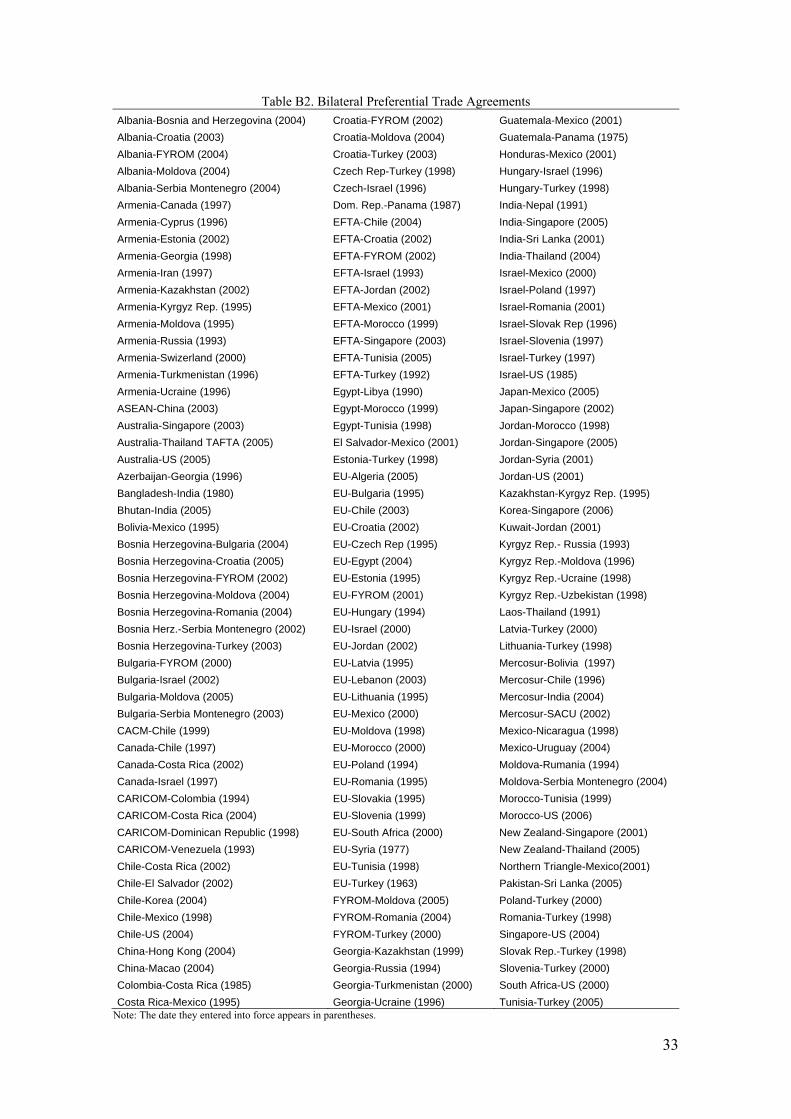
Table B2. Bilateral Preferential Trade Agreements Albania-Bosnia and Herzegovina (2004) Croatia-FYROM (2002) Guatemala-Mexico (2001) Albania-Croatia (2003) Croatia-Moldova (2004) Guatemala-Panama (1975) Albania-FYROM (2004) Croatia-Turkey (2003) Honduras-Mexico (2001) Albania-Moldova (2004) Czech Rep-Turkey (1998) Hungary-Israel (1996) Albania-Serbia Montenegro (2004) Czech-Israel (1996) Hungary-Turkey (1998) Armenia-Canada (1997) Dom. Rep.-Panama (1987) India-Nepal (1991) Armenia-Cyprus (1996) EFTA-Chile (2004) India-Singapore (2005) Armenia-Estonia (2002) EFTA-Croatia (2002) India-Sri Lanka (2001) Armenia-Georgia (1998) EFTA-FYROM (2002) India-Thailand (2004) Armenia-Iran (1997) EFTA-Israel (1993) Israel-Mexico (2000) Armenia-Kazakhstan (2002) EFTA-Jordan (2002) Israel-Poland (1997) Armenia-Kyrgyz Rep. (1995) EFTA-Mexico (2001) Israel-Romania (2001) Armenia-Moldova (1995) EFTA-Morocco (1999) Israel-Slovak Rep (1996) Armenia-Russia (1993) EFTA-Singapore (2003) Israel-Slovenia (1997) Armenia-Swizerland (2000) EFTA-Tunisia (2005) Israel-Turkey (1997) Armenia-Turkmenistan (1996) EFTA-Turkey (1992) Israel-US (1985) Armenia-Ucraine (1996) Egypt-Libya (1990) Japan-Mexico (2005) ASEAN-China (2003) Egypt-Morocco (1999) Japan-Singapore (2002) Australia-Singapore (2003) Egypt-Tunisia (1998) Jordan-Morocco (1998) Australia-Thailand TAFTA (2005) El Salvador-Mexico (2001) Jordan-Singapore (2005) Australia-US (2005) Estonia-Turkey (1998) Jordan-Syria (2001) Azerbaijan-Georgia (1996) EU-Algeria (2005) Jordan-US (2001) Bangladesh-India (1980) EU-Bulgaria (1995) Kazakhstan-Kyrgyz Rep. (1995) Bhutan-India (2005) EU-Chile (2003) Korea-Singapore (2006) Bolivia-Mexico (1995) EU-Croatia (2002) Kuwait-Jordan (2001) Bosnia Herzegovina-Bulgaria (2004) EU-Czech Rep (1995) Kyrgyz Rep.- Russia (1993) Bosnia Herzegovina-Croatia (2005) EU-Egypt (2004) Kyrgyz Rep.-Moldova (1996) Bosnia Herzegovina-FYROM (2002) EU-Estonia (1995) Kyrgyz Rep.-Ucraine (1998) Bosnia Herzegovina-Moldova (2004) EU-FYROM (2001) Kyrgyz Rep.-Uzbekistan (1998) Bosnia Herzegovina-Romania (2004) EU-Hungary (1994) Laos-Thailand (1991) Bosnia Herz.-Serbia Montenegro (2002) EU-Israel (2000) Latvia-Turkey (2000) Bosnia Herzegovina-Turkey (2003) EU-Jordan (2002) Lithuania-Turkey (1998) Bulgaria-FYROM (2000) EU-Latvia (1995) Mercosur-Bolivia (1997) Bulgaria-Israel (2002) EU-Lebanon (2003) Mercosur-Chile (1996) Bulgaria-Moldova (2005) EU-Lithuania (1995) Mercosur-India (2004) Bulgaria-Serbia Montenegro (2003) EU-Mexico (2000) Mercosur-SACU (2002) CACM-Chile (1999) EU-Moldova (1998) Mexico-Nicaragua (1998) Canada-Chile (1997) EU-Morocco (2000) Mexico-Uruguay (2004) Canada-Costa Rica (2002) EU-Poland (1994) Moldova-Rumania (1994) Canada-Israel (1997) EU-Romania (1995) Moldova-Serbia Montenegro (2004) CARICOM-Colombia (1994) EU-Slovakia (1995) Morocco-Tunisia (1999) CARICOM-Costa Rica (2004) EU-Slovenia (1999) Morocco-US (2006) CARICOM-Dominican Republic (1998) EU-South Africa (2000) New Zealand-Singapore (2001) CARICOM-Venezuela (1993) EU-Syria (1977) New Zealand-Thailand (2005) Chile-Costa Rica (2002) EU-Tunisia (1998) Northern Triangle-Mexico(2001) Chile-El Salvador (2002) EU-Turkey (1963) Pakistan-Sri Lanka (2005) Chile-Korea (2004) FYROM-Moldova (2005) Poland-Turkey (2000) Chile-Mexico (1998) FYROM-Romania (2004) Romania-Turkey (1998) Chile-US (2004) FYROM-Turkey (2000) Singapore-US (2004) China-Hong Kong (2004) Georgia-Kazakhstan (1999) Slovak Rep.-Turkey (1998) China-Macao (2004) Georgia-Russia (1994) Slovenia-Turkey (2000) Colombia-Costa Rica (1985) Georgia-Turkmenistan (2000) South Africa-US (2000) Costa Rica-Mexico (1995) Georgia-Ucraine (1996) Tunisia-Turkey (2005)

Note: The date they entered into force appears in parentheses.

33

34

Table B3. Currency Unions Multilateral CUs

Abbreviation Name of CU Stars/ends Member countries

EURO European Monetary Union 1999 Austria, Belgium-Luxembourg, Finland, France, Germany, Ireland, Italy, Netherlands, Portugal, Spain, Greece (joined 2001).

WAEMU/UEMOA West African Economic and Monetary Union

1962 Benin (joined 1984), Burkina Faso, Cotê d'Ivoire, Guinea-Bissau (joined 1996), Mali, Niger, Senegal, Mauritania (left 1995), Togo (joined 1996).

CEMAC/CAEMC (former UDEAC)

Economic and Monetary Union of Central Africa

1999 Cameroon, Central African Republic, Chad (left 1967, joined again 1984), Rep. of the Congo, Equatorial Guinea (joined 1984) and Gabon.

CMA Common Monetary Area 1960 Bostwana (left 1973), Lesotho, Namibia, Swaziland, South Africa.

EASTCARIBEAN East Caribbean Dollar 1965 Antigua and Barbuda, Barbados (left 1974), Dominica, Grenada, Guyana (left 1972), St. Kitts and Nevis, Sta. Lucia, St. Vincent, Trinidad and Tobago (left 1976).

Bilateral CUs

Abbreviation Stars/ends Member countries ARU_NA 1960-1993 Aruba and Netherland Antilles ARG_US 1992-2001 Argentina and United States AUL_KIR 1980 Australia and Kiribati AUL_TON 1960-1990 Australia and Tonga AUL_SOL 1978 Australia and Solomon Islands BAH_US 1966 Bahamas and United States BER_US 1970 Bermuda and United States ECU_US 2001 Ecuador and United States HK_US 1984 Hong Kong and United States IND_BHU 1991 India and Bhutan PAN_US 1904 Panama and United States QAT_UAE 1981 Qatar and United Arab Emirates