io long waves ocean tides the main purpose of this · pdf filewaves and ocean tides around...

IOLong Waves andOcean Tides

Myrl C. Hendershott

10.1 Introduction

The main purpose of this chapter is to summarize whatwas generally known to oceanographers about longwaves and ocean tides around 1940, and then to indi-cate how the subject has developed since then, withparticular emphasis upon those aspects that have hadsignificance for oceanography beyond their importancein understanding tides themselves. I have begun witha description of astronomical and radiational tide-gen-erating potentials (section 10.2), but say no more thanis necessary to make this chapter self-contained. Cart-wright (1977) summarizes and documents recent de-velopments, and I have followed his discussion closely.

The fundamental dynamic equations governing tidesand long waves, Laplace's tidal equations (LTE), re-mained unchanged and unchallenged from Laplace'sformulation of them in 1776 up to the early twentiethcentury. By 1940 they had been extended to allow fordensity stratification (in the absence of bottom relief)and criticized for their exclusion of half of the Coriolisforces. Without bottom relief this exclusion has re-cently been shown to be a good approximation; thedemonstration unexpectedly requires the strong strat-ification of the ocean. Bottom relief appears able tomake long waves in stratified oceans very differentfrom their flat-bottom counterparts (section 10.4); adefinitive discussion has not yet been provided. Finally,LTE have had to be extended to allow for the gravita-tional self-attraction of the oceans and for effects dueto the tidal yielding of the solid earth. I review thesematters in section 10.3.

Laplace's study of the free oscillations of a globalocean governed by LTE was the first study of oceaniclong waves. Subsequent nineteenth- and twentieth-century explorations of the many free waves allowedby these equations, extended to include stratification,have evolved into an indispensible part of geophysicalfluid dynamics. By 1940, most of the flat-bottom so-lutions now known had, at least in principle, beenconstructed. But Rossby's rediscovery and physical in-terpretation, in 1939, of Hough's oscillations of thesecond class began the modem period of studying so-lutions of the long-wave equations by inspired or sys-tematic approximation and of seeking to relate theresults to nontidal as well as tidal motions. Since then,flat-bottom barotropic and baroclinic solutions of LTEhave been obtained in mid-latitude and in equatorialapproximation, and Laplace's original global problemhas been completely solved. The effects of bottom re-lief on barotropic motion are well understood. Signifi-cant progress has been made in understanding the ef-fects of bottom relief on baroclinic motions. I haveattempted to review all those developments in a self-contained manner in section 10.4. In order to treat this

292Myrl C. Hendershott

�1 _·� �IC� _ __��_

vast subject coherently, I have had to impose my ownview of its development upon the discussion. I havecited observations when they appear to illustrate someproperty of the less familiar solutions, but the centraltheme is a description of the properties of theoreticallypossible waves of long period (greater than the buoy-ancy period) and, consequently, of length greater thanthe ocean's mean depth.

Although the study of ocean surface tides was theoriginal study of oceanic response to time-dependentforcing, tidal studies have largely proceeded in isolationfrom modem developments in oceanography on ac-count of the strength of the tide-generating forces, theirwell-defined discrete frequencies, and the proximity ofthese to the angular frequency of the earth's rotation.A proper historical discussion of the subject, althoughof great intellectual interest, is beyond the scope ofthis chapter. To my mind the elements of such a dis-cussion, probably reasonably complete through thefirst decade of this century, are given in Darwin's 1911Encyclopedia Britannica article "Tides." Thereafter,with a few notable exceptions, real progress had toawait modem computational techniques both for solv-ing LTE and for making more complete use of tidegauge observations. Cartwright (1977) has recently re-viewed the entire subject, and therefore I have given adiscussion in section 1].0.5 that, although self-con-tained, emphasizes primarily changes of motivationand viewpoint in tidal studies rather than recapitulatesCartwright's or other recent reviews.

This discussion of tides as long waves continuouslyforced by lunar and solar gravitation logically could befollowed by a discussion of tsunamis impulsivelyforced by submarine earthquakes. But lack of bothspace and time has forced omission of this topic.

Internal tides were first reported at the beginning ofthis century. By 1940 a theoretical framework for theirdiscussion had been supplied by the extension of LTEto include stratification, and their generation was(probably properly) ascribed to scattering of barotropictidal energy from bottom relief. The important devel-opments since then are recognition of the intermittentnarrow-band nature of internal tides (as opposed to thenear-line spectrum of surface tides) plus the beginningsof a statistically reliable characterization of the inter-nal tidal spectrum and its variation in space and time.The subject has recently been reviewed by Wunsch(1975). Motivation for studying internal tides hasshifted from the need for an adequate description ofthem through exploration of their role in global tidaldissipation (now believed to be under 10%) to specu-lation about their importance as energy sources foroceanic mixing. In section 10.6 I have summarizedmodem observational studies and their implicationsfor tidal mixing of the oceans.

Many features of the presentday view of ocean cir-culation have some precedent in tidal and long-wavestudies, although often unacknowledged and appar-ently not always recognized. The question of whichparts of the study of tides have in fact influenced thesubsequent development of studies of ocean circulationis a question for the history of science. In some cases,developments in the study of ocean circulation subse-quently have been applied to ocean tides. In section10.7 I have pointed out some of the connections ofwhich I am aware.

10.2 Astronomical Tide-Generating Forces

Although correlations between ocean tides and the po-sition and phase of the moon have been recognized andutilized since ancient times, the astronomical tide-gen-erating force (ATGF) was first explained by Newton inthe Principia in 1687. Viewed in an accelerated coor-dinate frame that moves with the center of the earthbut that does not rotate with respect to the fixed stars,the lunar (solar) ATGF at any point on the earth'ssurface is the difference between lunar (solar) gravita-tional attraction at that point and at the earth's center.The daily rotation of the earth about its axis carries aterrestrial observer successively through the longitudeof the sublunar or subsolar point [at which the lunar(solar) ATGF is toward the moon (sun)] and then halfa day later through the longitude of the antipodal point[at which the ATGF is away from the moon (sun)]. InNewton's words, "It appears that the waters of the seaought twice to rise and twice to fall every day, as welllunar or solar" [Newton, 1687, proposition 24, theorem19].

The ATGF is thus predominantly semidiurnal withrespect to both the solar and the lunar day. But it isnot entirely so. Because the tide-generating bodies arenot always in the earth's equatorial plane, the terres-trial observer [who does not change latitude whilebeing carried through the longitude of the sublunar(solar) point or its antipode] sees a difference in ampli-tude between the successive semidiumal maxima ofthe ATGF at his location. This difference or "dailyinequality" means that the ATGF must be thought ofas having diurnal as well as semidiurnal time variation.

Longer-period variations are associated with period-icities in the orbital motion of earth and moon. Theastronomical variables displaying these long-periodvariations appear nonlinearly in the ATGF. The long-period orbital variations thus interact nonlinearly bothwith themselves and with the short-period diurnal andsemidiurnal variation of the ATGF to make the localATGF a sum of three narrow-band processes centeredabout 0, 1, and 2 cycles per day (cpd), each processbeing a sum of motions harmonic at multiples 0,1,2 ofthe frequencies corresponding to a lunar or a solar day

293Long Waves and Ocean Tides

plus sums of multiples of the frequencies of long-periodorbital variations.

A complete derivation of the ATGF is beyond thescope of this discussion. Cartwright (1977) reviews thesubject and supplies references documenting its mod-ern development. For a discussion that concentratesupon ocean dynamics (but not necessarily for a prac-tical tide prediction), the most convenient representa-tion of the ATGF is as a harmonic decomposition ofthe tide-generating potential whose spatial gradient isthe ATGF. Because only the horizontal components ofthe ATGF are of dynamic importance, it is convenientto represent the tide-generating potential by its hori-zontal and time variation U over some near-sea-levelequipotential (the geoid) of the gravitational potentialdue to the earth's shape, internal mass distribution,and rotation. To derive the dynamically significant partof the ATGF it suffices to assume this surface spheri-cal. U/g (where g is the local gravitational constant,unchanging over the geoid) has the units of sea-surfaceelevation and is called the equilibrium tide . Its prin-ciple term is (Cartwright, 1977)

,OEt) = U(,O,t)g

= Y (Amcosm4 + B sinm)Pz', (10.1)m=0.12

in which 4A,O are longitude and latitude, the P-() areassociated Legendre functions

P0 = (3 cos2 - 1),

P = 3 sin6 cos ,

the N}'1 are sets of small integers (effectively the Dood-son numbers); and the S,(t) are secular arguments thatincrease almost linearly in time with the associatedperiodicity of a lunar day, a sidereal month, a tropicalyear, 8.847 yr (period of lunar perigee), 18.61 yr (periodof lunar node), 2.1 x 104 yr (period of perihelion), re-spectively.

The frequencies of the arguments XNi' Sj(t) fall intothe three "species"-long period, diurnal, and semidi-urnal-which are centered, respectively, about 0, 1, and2 cpd (N1 = 0,1,2). Each species is split into "groups"separated by about 1 cycle per month, groups are splitinto "constituents" separated by one cyle per year, etc.Table 10.1 lists selected constituents. In the followingdiscussion they are referred to by their Darwin symbol(see table 10.1).

An important development in modern tidal theoryhas been the recognition that the ATGF is not the onlyimportant tide-generating force. Relative to the ampli-tudes and phases of corresponding constituents of theequilibrium tide, solar semidiurnal, diurnal, and an-nual ocean tides usually have amplitudes and phasesquite different from the amplitudes and phases of othernearby constituents. Munk and Cartwright (1966) at-tributed these anomalies in a general way to solar heat-ing and included them in a generalized equilibriumtide by defining an ad hoc radiational potential (Cart-wright, 1977)

UR(+, ,t) = { S(/1) cosa,0,(10.2)

P2 = 3 sin 2 0

of colatitude 8 = (r/2) - 0, and A2m, B 2 are functions oftime having the form

A (t) = EXMics [ N"Si(tJ)]. (10.3)

The MI are amplitudes obtained from Fourier analysisof the astronomically derived time series U(,0O,t)/g;

0 < a < r/2:

7r/2 < a < r:(10.4)

which is zero at night, which varies as the cosine ofthe sun's zenith angle a during the day, and which isproportional to the solar constant S and the sun's par-allax 6 (mean f). Cartwright (1977) suggests that for theoceanic S2 (principal solar) tide, whose anomalous por-tion is about 17% of the gravitational tide (Zetler,1971), the dominant nongravitational driving is by theatmospheric S2 tide. Without entering further into thediscussion, I want to point out that the global form of

Table 10.1 Charactenstlcs of Selected Constituents of the Equilibrium Tide

PeriodDarwin (solar days Amplitude M Spatialsymbol N1, N 2, N3, N 4 or hours) (m) variation

S 0 0 2 0 182.621 d 0.02936Mm 0 1 0 -1 27.55 d 0.03227 ½(3 cos2 - 1)M, 0 2 0 0 13.661 d 0.06300, 1 -1 0 0 25.82 h 0.06752P, 1 1 -2 0 24.07 h 0.03142 3sin0cos0 x sin(wt + k)Kl 1 1 0 0 23.93 h 0.09497N 2 2 -1 0 1 12.66 h 0.01558M2 2 0 0 0 12.42 h 0.08136 3sin28 x cos(w2t + 20)S2 2 2 -2 0 12.00 h 0.03785K 2 2 2 0 0 11.97 h 0.01030


the atmospheric S2 tide is well known (Chapman andLindzen, 1970), so that the same numerical programsthat have been used to solve for global gravitationallydriven ocean tides could easily be extended to allowfor atmospheric-pressure driving of the oceanic S2 tide.

Ocean gravitational self-attraction and tidal solid-earth deformation are quantitatively even more impor-tant in formulating the total tide-generating force thanare thermal and atmospheric effects. They are dis-cussed in the following section, since they bring abouta change in the form of the dynamic equations govern-ing ocean tides.

10.3 Laplace's Tidal Equations (LTE) and the Long-Wave Equations

Laplace (1775, 1776; Lamb, 1932, §213-221) cast thedynamic theory of tides essentially in its modem form.His tidal equations (LTE) are usually formally obtainedfrom the continuum equations of momentum and massconservation (written in rotating coordinates for a fluidshell surrounding a nearly spherical planet and havinga gravitationally stabilized free surface) by assuming(Miles, 1974a)

(1) a perfect homogeneous fluid,(2) small disturbances relative to a state of uniformrotation,(3) a spherical earth,(4) a geocentric gravitational field uniform horizon-tally and in time,(5) a rigid ocean bottom,(6) a shallow ocean in which both the Coriolis accel-eration associated with the horizontal component ofthe earth's rotation and the vertical component of theparticle acceleration are neglected.

The resulting equations are

0- - 2f sin v = --h( ~ - r/g)/a cos0, (10.5a)

-t + 2sinOu = -- ( - /g)/a, (10.5b)

+ 1 (u D) + (vD cos)] = 0. (10.5c)It a cos r0 ce

In these, (, ) are longitude and latitude with corre-sponding velocity components (u, v), the ocean sur-face elevation, F the tide-generating potential, D(0, )the variable depth of the ocean, a the earth's sphericalradius, g the constant gravitational attraction at theearth's surface, and 12 the earth's angular rate of rota-tion.

Two modern developments deserve discussion. Theyare a quanitative formulation and study of the mathe-matical limit process implicit in assumptions (1)through (6), and the realization that assumptions (4)

and (5) are quantitatively inadequate for a dynamicdiscussion of ocean tides.

It has evidently been recognized since the work ofBjerknes, Bjerknes, Solberg, and Bergeron (1933) thatassumption (6) (especially the neglect of Coriolis forcesdue to the horizontal component of the earth's rota-tion) amounts to more than a minor perturbation ofthe spectrum of free oscillations that may occur in athin homogeneous ocean. Thus Stern (1963) and Israeli(1972) found axisymmetric equatorially trapped normalmodes of a rotating spherical shell of homogeneousfluid that are extinguished by the hydrostatic approx-imation. Indeed, Stewartson and Rickard (1969) pointout that the limiting case of a vanishingly thin ho-mogeneous ocean is a nonuniform limit: the solutionsobtained by solving the equations and then taking thelimit may be very different from those obtained by firsttaking the limit and then solving the resulting approx-imate (LTE) equations. Quite remarkably, it is the rein-statement of realistically large stratification, i.e., therelaxation of assumption (1), that saves LTE as an ap-proximate set of equations whose solutions are uni-formly valid approximations to some of the solutionsof the full equations when the ocean is very thin.

The parodoxical importance of stratification for thevalidity of the ostensibly unstratified LTE appears tohave been recognized by Proudman (1948) and byBretherton (1964). Phillips (1968) pointed out its im-portance at the conclusion of a correspondence withVeronis (1968b) concerning the effects of the "tradi-tional" approximation (Eckart, 1960; N. A. Phillips,1966b), i.e., the omission of the Coriolis terms2t cosOw and -2flcosOu, in (10.6)-(10.8) below. Butit was first explicitly incorporated into the limit proc-ess producing LTE by Miles (1974a) who addressed allof assumptions (1) through (6) by defining appropriatesmall parameters and examining the properties of ex-pansions in them. He found that the simplest set ofuniformly valid equations for what I regard as longwaves in this review are

-- 21 sin Ov + 2 cos Ow = p 1at a p 0alcos0 '

v + 2 sin Ou - p Iat O0 poa

Ou 0 2p 1N2w - 21 cos 0A- ip at az at p0 '

au a(v cos ) aw- + + a cos - = 0,'go a6 az

with boundary conditions

w =0 at z = -D,

(for uniform depth D),

(10.6a)

(10.6b)

(10.6c)

(10.6d)

(10.7)


p = - 0 g 0 at z = 0. (10.8)

In these, z is the upward local vertical with associatedvelocity component w, p the deviation of the pressurefrom a resting hydrostatic state characterized by thestable density distribution p,(z), p a constant charac-terizing the mean density of the fluid (the Boussinesqapproximation has been made in its introduction); thebuoyancy frequency

/g Opo g:2\ 121

N{z = ( Po Oz C2) .9)

is the only term in which allowance for compressi-bility ({c is the local sound speed) is important in theocean.

Miles (1974a) further found that when N2(z) >> 42,free solutions of LTE for a uniform-depth (D) oceancovering the globe also solve (10.6)-(10.8) with an errorwhich is of order la/2f1)(412a/g) << 1, where a is thefrequency of oscillation of the free solutions. LTE sur-face elevations are consequently in error by order(D/a)(DN 2 /g)-314 , while LTE velocities u,v may be inerror by (D/a)(D N2 /g)- 4. Miles (1974a) obtained thisresult by taking the (necessarily barotropic) solutionsof LTE as the first term of an expansion of the solutionsof (10.6)-(10.8) in the parameter (a/21f)(4112a/g), whichturns out to characterize the relative importance ofterms neglected and terms retained in making assump-tion (6). The next term in the expansion consists ofinternal wave modes (see section 10.4.3). Because theirfree surface displacements are very small relative tointernal displacements, the overall free surface dis-placement remains as in LTE although in the interiorof the ocean, internal wave displacements and currentsmay well dominate the motion.

The analysis is inconclusive at frequencies or depthsat which the terms assumed to be correction pertur-bations are resonant. Finding expressions for all thefree oscillations allowed by Miles's simplest uniformlyvalid system (10.6)-(10.8) involves as yet unresolvedmathematical difficulties associated with the fact thatthese equations are hyperbolic over part of the spatialdomain when the motion is harmonic in time (Miles,1974a).

Application of this analysis to ocean tides is furthercircumscribed by its necessary restriction to a globalocean of constant depth. I speculate that if oceanicinternal modes are sufficiently inefficient as energytransporters that they cannot greatly alter the energet-ics of the barotropic solution unless their amplitudesare resonantly increased beyond observed levels (sec-tion 10.6), and if they are sufficiently dissipative thatthey effectively never are resonant, then an extensionof this analysis to realistic basins and relief wouldprobably confirm LTE as adequate governors of thesurface elevation. The ideas, necessary for such an

extension, that is, how variable relief and stratificationinfluence barotropic and baroclinic modes, are begin-ning to be developed (see section 10.4.7).

Miles (1974a) discusses assumptions (3)-(5) with ex-plicit omission of ocean gravitational self-attractionand solid-earth deformation. Self-attraction was in-cluded in Hough's (1897, 1898; Lamb, 1932, §222-223)global solutions of LTE. Thomson (1863) evidently firstpointed out the necessity of allowing for solid-earthdeformation. Both are quantitatively important. Thelatter manifests itself in a geocentric solid-earth tide 8plus various perturbations of the total tide-generatingpotential F. Horizontal pressure gradients in LTE (10.5)are associated with gradients of the geocentric oceantide , but it is the observed ocean tide

(10.10)

that must appear in the continuity equation of (10.5c).All these effects are most easily discussed (although

not optimally computed) when the astronomical po-tential U, the observed ocean tide 50, the solid earthtide 8, and the total tide-generating potential r are alldecomposed into spherical harmonic components U,0n, ,, and Fr. The Love numbers k,, h,, ki, h, which

carry with them information about the radial structureof the solid earth (Munk and McDonald, 1960), and theparameter an = (3/2n + l)(ocean/PeartI) then appear nat-urally in the development. The total tide-generatingpotential rF contains an astronomical contribution Un(primarily of order n = 2), an augmentation knUn ofthis due to solid earth yielding to -VU,, an oceanself-attraction contribution ga,,,on, and a contributionkgan;n due to solid-earth deformation by ocean self-attraction and tidal column weight. Thus

rF = (1 + k,,)U + 1 + k)gan<,0,. (10.11)

There is simultaneously a geocentric solid-earth tide8 made up of the direct yielding hnUg of the solidearth to -VUn plus the deformation h'ganon of thesolid earth by ocean attraction and tidal columnweight. Thus

8n = hnU,/g + hngaton. (10.12)

For computation, Farrell (1972a) has constructed aGreen's function such that

{ (1 + k - h)an,,

= ff do' d,' cos 0' G(4 ,'lro)Wolo').ocean

(10.13)

With U = U2 and with (10.13) abbreviated as IffGG,LTE with assumptions (4) and (5) appropriately relaxedbecome


<0 = - 8

au - 2sinOv = [ - - (1 + k2 - h2)U2 gat a cos 0 0a

-| Go] (10.14,Ov gOeV + 2flsinOu = - 1 + k2 - h2)U2/gat ~ a 0

-ff Go], (10.14

du + 1 [a(uD) a(vDcose)] = . (10.14at a cos + : 0. 10.14

10.4 Long Waves in the Ocean

10.4.1 Introduction

a) The first theoretical study of oceanic long waves is dueto Laplace (1775, 1776; Lamb, 1932, §213-221), whosolved LTE for an appropriately shallow ocean coveringa rotating rigid spherical earth by expanding the solu-tion in powers of sin 0. For a global ocean of constantdepth D., Hough (1897, 1898; Lamb, 1932, §222-223)

b) obtained solutions converging rapidly for small

A = 4fQ2a2/gD,

c)

The factor 1 + k2 - h2 = 0.69 is clearly necessary fora quantitatively correct solution. The term fJfGo wasfirst evaluated by Farrell (1972b). I wrote down (10.14)and attempted to estimate the effect of fGCo on aglobal numerical solution of (10.14) for the M2 tide byan iterative procedure which, however, failed to con-verge (Hendershott, 1972). Subsequent computationsby Gordeev, Kagan, and Polyakov (1977) and by Accadand Pekeris (1978) provide improved estimates of theeffects (see section 10.5.3).

With appropriate allowance for various dissipativeprocesses (including all mechanisms that put energyinto internal tides), I regard (10.14) as an adequate ap-proximation for studying the ocean surface tide.Oceanic long waves should really be discussed using(10.6) but allowing for depth variations by putting

w = u'VD at z = -D(,0) (10.15)

in place of (10.7). Miles (1974a) derives an orthogonalityrelationship that could be specialized to (10.6)-(10.8)in the case of constant depth, but even then the non-separability of the eigenfunctions into functions of (, 0)times functions of z has prevented systematic study ofthe problem. Variable relief compounds the difficulty.Most studies either deal with surface waves over bot-tom relief, and thus start with LTE (10.5), or else withsurface and internal waves over a flat bottom. In thelatter case, (10.6)-(10.8) are solved but with the Coriolisterms 2 cos Ow and -212 cos Ou arbitrarily neglected(the "traditional" approximation). Miles' (1974a) re-sults appear to justify this procedure for the formercase, but Munk and Phillips (1968) show that the ne-glected terms are proportional to (mode number) 13 forinternal modes so that the traditional approximationmay be untenable for high-mode internal waves. Thefollowing discussion (section 10.4) of oceanic longwaves relies heavily upon the traditional approxima-tion, but it is important to note that its domain ofvalidity has not yet been entirely delineated.

(sometimes called Lamb's parameter) by expanding thesolution in spherical harmonics PI (sin 0) expi14). Hefound the natural oscillations to be divided into first-and second-class modes whose frequencies r are given,respectively, by

= -+[n(n + l)gD/a 2]1 '2,

= -21ll/[n(n + 1)]

as A- 0. But A - 20 for D. = 4000 m, and is verymuch larger for internal waves (see section 10.4.3). Acorrespondingly complete solution of Laplace's prob-lem, valid for large as well as small A, was given onlyrecently (Flattery, 1967; Longuet-Higgins, 1968a).Physical understanding of the solutions has historicallybeen developed by studying simplified models of LTE.

10.4.2 Long Waves in Uniformly Rotating Flat-Bottomed OceansLord Kelvin (Thomson, 1879; Lamb, 1932, §207) intro-duced the idealization of uniform rotation, at fl, of asheet of fluid about the vertical (z-axis). LTE become

au dt;at f0o --g

av - gat * fou = - g a9Cat - v04 a(uD) a(vD)

+ + = 0.at ax ay

f0, here equal to 2, is the Coriolis parameter. LordKelvin's plane model (10.18) is often called the f-plane.

The solid earth is nearly a spheroid of.equilibriumunder the combined influence of gravity g and centrif-ugal acceleration f12a; the earth's equatorial radius isabout 20 km greater than its polar radius. Withoutwater motion, the sea surface would have a congruentspheroidal shape. Taking the depth constant in LTEmodels this similarity; the remaining error incurred byworking in spherical rather than spheroidal coordinatesis (Miles, 1974a) of order W12a/g = 10- 3. It is correspond-ingly appropriate to take the depth constant in LordKelvin's plane model (10.18) in order to obtain planar


(10.16)

(10.17)

(10.18a)

(10.18b)

(110.18c)

- - -

solutions locally modeling those of LTE with constantdepth. But the laboratory configuration correspondingto constant depth in (10.18c) is a container with aparaboloidal bottom Yfl2 x2 + y2)/g rather than a flatbottom [see Miles (1964) for a more detailed analysis].

Without rotation (fo = 0) and with constant depth(D = D*) Lord Kelvin's plane model reduces to thelinearized shallow-water equations (LSWE). For anunbounded fluid sheet, they have plane gravity-wavesolutions

= a exp(-irot + ilx + iky), (10.19a)

u = (gl/C, (10.lob)

v = (gk/lr), (10.19c)

w =-ir(z/D, + 1)4, (10.19d)a2 = gD(12 + k2), (10.19e)

which are dispersionless [all travel at (gD)112] and arelongitudinal [(u, v) parallel to (1, k)]. Horizontal particleaccelerations are exactly balanced by horizontal pres-sure-gradient forces while vertical accelerations arenegligible. Such waves reflect specularly at a straightcoast with no phase shift; thus

5 = a exp(-io-t + ilx + iky)

+ a exp(-ia-t - ilx + iky)

satisfies u = 0 at the coast x = 0, the angle taof incidence equals the angle of reflection, (complex) reflected amplitude equals the incideplitude a. The normal modes of a closed basiperimeter P are the eigensolutions Z.(x,y)expa(T of

VlZn + (rnlgD*)Zn = 0

with

OZ/dO(normal) = 0 on P.

If P is a constant surface in one of the coordinatems in which V22 separates, then the normal mcmathematically separable functions of the twzontal space coordinates and so are readily disin terms of appropriate special functions. Eveneral basin shapes, the existence and completethe normal modes are assured (Morse and Fes1953).

With rotation, plane wave solutions of (10. 1constant depth D are

5 = a exp(--it + ilx + iky),

u = g[(lar + ikfo)/(r-2 - f)1;,

v = g[(kar - ilfo)/(a2 - fA)],

w = -iozlD, + 1)5,

(10.20)

Ln-(k/l)md thent am-

in with(-iejt),

2 = gD(1 2 + k2 ) + f. (10.23e)

These are often called Sverdrup waves (apparently afterSverdrup, 1926). Rotation has made them dispersiveand they propagate only when ao > f. The group ve-locity cg = (Or/01, 9or/k) is parallel to the wavenumberand rises from zero at or = f0 toward (gD,) 2 as o2 >>

fo. Dynamically these waves are LSW waves perturbedby rotation. Particle paths are ellipses with ratio f/cr ofminor to major axis and with major axis oriented along(1,k). Particles traverse these paths in the clockwisedirection (viewed from above) when f > 0 (northernhemisphere). Sverdrup waves are reflected specularlyat a straight coast but with a phase shift; the sum

5 = a exp(io-t + ilx + iky)

+a[(la + ikfo)I(lr - ikfo)]

x exp (-io-t - ilx + iky) (10.24)

of two Sverdrup waves satisfies u = 0 at the coastx = 0, the angle tan-(k/l) of incidence equals the angleof reflection, and the reflected amplitude differs fromthe incident amplitude by the multiplicative constant(Icr + ikfo)/(la - ikfo), which is complex but of modulusunity. The sum (10.24) is often called a Poincar6 wave.The normal modes of a closed basin with perimeter Pare the eigensolutions Z,(x,y) exp( -iaet), a- of

V2Z. + [(Cr2 - f2o)/gD*]Z = 0

with

-ir,, OZJ/O(normal)

+ fo Znla(tangent) = 0 at P.

(10.25)

(10.26)

On account of the boundary condition (10.26), they are(10.21) not usually separable functions of the two horizontal

space coordinates. The circular basin (Lamb, 1932,§209-210) is an exception. Rao (1966) discusses the

(10.22) rectangular basin, but the results are not easily sum-ite sys- marized. A salient feature, the existence of free oscil-ides are lations with o2 < f2, is rationalized below.

o hori- With rotation, Lord Kelvin (Thomson, 1879; Lamb,;cussed 1932, §208) showed that a coast not only reflects Sver-

in gen- drup waves for which o2 > f, but makes possible aness of new kind of coastally trapped motion for which Ca2 2,.hl. f . This Kelvin wave has the form

U) with1,

8) with

(10.23a)

(10.23b)

(10.23c)

= a exp[-io-t + iky + k(fol/r)x],

u = 0,

v = (gk/or)

w = -iazlD, + 1)4,

a2 =gDk 2

(10.27a)

(10.27b)

(10.27c)

(10.27d)

(10.27e)

(10.23d) along the straight coast x = 0. The velocity normal tothe coast vanishes everywhere in the fluid and not only


�_�__ __ �___II _ I_

at the coast. The wave is dispersionless and propagatesparallel to the shore with speed (gD,)1x2 for 0.2 2 f{ justlike a longitudinal gravity wave but with an offshoreprofile exp[k(fo/o)x] that decays or grows exponentiallyseaward depending upon whether the wave propagateswith the coast to its right or to its left (in the northernhemisphere, f > 0). For vanishing rotation, the offshoredecay or growth scale becomes infinite and the Kelvinwave reduces to an ordinary gravity wave propagatingparallel to the coast. The Kelvin wave is dynamicallyexactly a LSW gravity wave in the longshore directionand is exactly geostrophic in the cross-shore direction.

A pair of Kelvin waves propagating in opposite di-rections along the two coasts of an infinite canal (at,say, x = 0 and x = W) gives rise to a pattern of sea-level variation in which the nodal lines that wouldoccur without rotation shrink to amphidromic points,at which the surface neither rises nor falls and aboutwhich crests and troughs rotate counterclockwise (inthe northern hemisphere) as time progresses. For equal-amplitude oppositely propagating Kelvin waves, theamphidromic points fall on the central axis of the canaland are separated by a half-wavelength (7rk-1). Whenthe amplitudes are unequal, the line of amphidromesmoves away from the coast along which the highest-amplitude Kelvin wave propagates. For a sufficientlygreat difference in amplitudes, the amphidromes mayoccur beyond one of the coasts, i.e., outside of thecanal.

Such a pair of Kelvin waves cannot by themselvessatisfy the condition of zero normal fluid velocity in aclosed canal (say at y = 3). Taylor (1921) showed howthis condition could be satisfied by adjoining to thepair of Kelvin waves an infinite sum of channel Poin-care modes

= [cos(m7rx/W) - (fo/0 )(kW/m7r)

x sin(mrrx/W)] exp[-.iot + iky],

a2 = (m2rT2/W2 + k2)gD, + f2, m = 1, 2,...,

(10.28)

than the channel width W, then the Poincar6 modessum to an appreciable contribution only near the cor-ners of the closure. The Kelvin wave then proceeds upthe channel effectively hugging one coast, turns thecorners of the closure with a phase shift [evaluated byBuchwald (1968) for a single comer], and returns backalong the channel hugging the opposite coast. Now itbecomes apparent that, with allowance for comerphase shifts, closed rotating basins have a class of freeoscillation whose natural frequencies are effectivelydetermined by fitting an integral number of Kelvinwaves along the basin perimeter. Such free oscillationsmay have or2 % f. They are readily identified in Lamb's(1932, §209-210) normal modes of a uniform-depth cir-cular basin.

10.4.3 The Effect of Density Stratification on LongWavesAll of the foregoing solutions are barotropic surfacewaves. Stokes (1847; Lamb, 1932, §231) pointed outthat surface waves are dynamically very much likewaves at the interfaces between fluid layers of differingdensities. Allowance for continuous vertical variationof density was made by Rayleigh (1883). Lord Kelvin'splane model (10.18) must be extended to read

-u fov = 1pat Po ox '

av 1 ap- + fou = ---

1 a2p

Po a at

au av aw- +- +- = 0,ax ay az

with

w =0 at z = -D,

(10.30a)

(10.30b)

(10.30c)

(10.30d)

(10.31)

and

each of which separately has vanishing normal fluidvelocity at the channel walls (x = O, W). These are justthe waveguide modes of the canal. Mode m decaysexponentially away from the closure (is evanescent) if

a2 < f2 + (m2,r2/W2)gD, . (10.29)

If o- is so low, W so small, or D so great that all modesm = 1, 2, . . . are evanescent, then the Kelvin waveincident on the closure has to be perfectly reflectedwith at most a shift of phase. When (10.29) is violatedfor the one or more lowest modes, then some of theenergy of the incident Kelvin wave is scattered intotraveling Poincare modes.

If (10.29) is satisfied for all m and if the decay scale(gD,)l/2/fo of the Kelvin waves is a good deal smaller

P = Og at z = 0. (10.32)

Notation is as in (10.6).For the case of constant depth D,, the principal result

is that the dependent variables have the separable form

(u,v,w,p) = {U(x,y,t), V(x,y,t), W(x,y,t),Z(x,y,t)}

(10.33)

where

W = aZ/at,

F, = F/Ipog = D,, Fw/z,

and

(10.34)


x JF.(z),F.(z),F.,(z ),F,(z ))T

au dZat fo = - x '

ov a =0,+ foU = -g-a--,

at- + aD. + ax 'I

with

2 Fw N2(z}d2 F2g + D Fw = 0,

Fw =0 at z = -D,,

F,,, - D OF,lz = 0 at z = 0. (10.38)

According to (10.35), the horizontal variations of allquantities are exactly as in the homogeneous flat bot-tom case except that now the apparent depth D, isobtained by solving the eigenvalue problem (10.36) forthe vertical structure. Typically (10.36) yields a baro-tropic mode F,,o z + D, Do = D plus an infinitesequence of baroclinic modes F,, characterized by nzero crossings (excluding the one at z = -D) and byvery small equivalent depths D,. Baroclinic WKB ap-proximate solutions (10.36)-(10.38) are

F.wz) = N-112 z) sin [ll /gDn) 112 N(z dz']

D,= [Y N(z')dz'1 (gn272).

These are exact for constant buoyancy frequeiForD, = 4000 m and N0 = 10l1, D, = (0.1/n2 ) mN(z) = No, it is easy to show that

[w at the free surface/interior maximum value

of w] = N&D,/n7rg << 1.

Free surface variation is thus qualitatively anctitatively unimportant for baroclinic modes. T]therefore usually called internal modes.

In a flat-bottomed ocean, stratification is thito make possible an infinite sequence of interrlicas of the barotropic LSW gravity waves, Siwaves, PoincarO waves, Kelvin waves, and basmal modes discussed above. All these except thewaves have a-2 > f,. They must also have a2over part of the water column, although the 1treatment does not make this obvious becauseN2 is always assumed. The horizontal variation creplicas is governed by the equations describibarotropic mode, except that the depth D, is fraction of the actual (constant) depth D. rotation, the speed of barotropic long gravity w(gD,)112 200 m s- in the deep sea. Long intern;ity waves move at the much slower (gD

(10.35a) (l/n) m s-. For comparable frequencies, the internalwaves thus have much shorter wavelength than thesurface wave.

(10.35b) An important point is that the separation of variables(10.33) works in spherical coordinates as well as inCartesian coordinates, provided only that the depth isconstant. The horizontal variation of flow variables isthen governed by LTE with appropriate equivalentdepth D, given by (10.36)-(10.38).

For plane waves of frequency or, relaxation of N 2 >>(10.36) or2 leads to the replacement of (10.36) by

(10.37) a2Fw [N 2(z) - or2]- + Fw = 0.arl

(10.39)

(10.41)6 'en

High-frequency waves, for which [N2(z) - or2] changessign over the water column, are discussed in chapter9.

The simplicity of these flat-bottom results is decep-tive, because they are very difficult to generalize toinclude bottom relief. The reason for this is most easilyseen by eliminating (u,v) from (10.30) for harmonicmotion [exp(-iot)] to obtain a single equation in w:

(10.42)w 2 No ( 02w 0 =02

_ _2 _ + a =.y2

This equation is hyperbolic in space for internal waves(for which f0 < a2 < N2,). Its characteristic surfaces are

z = +(2 + y2 )112(c 2 - o)'2lNo. (10.43)

Solutions of (10.42) may be discontinuous across char-acteristic surfaces, and they depend very strongly uponthe relative slope of characteristics and bounding sur-faces. Without rotation, internal waves of frequency aare solutions of the hyperbolic equation

(10.40) 82p (No- a2) ( 2 p a2p 02 UP i sty2, )nI quan-.1 ...... with the simple condition

Op =0 at solid boundaries.an

(10.44)

(10.45)

For closed boundaries (i.e., a container filled with strat-ified fluid) this is an ill-posed problem in the sense thattiny perturbations of the boundaries may greatly alterthe structure of the solutions. Horizontal boundaries,although analytically tractable, are a very special case.

10.4.4 Rossby and Planetary WavesIn an influential study whose emphasis upon physicalprocesses marks the beginning of the modern period,Rossby and collaborators (1939) rediscovered Hough'ssecond-class oscillations and suggested that they mightbe of great importance in atmospheric dynamics (seealso chapters 11 and 18).


Perhaps of even greater influence than this discoverywas Rossby's creation of a new plane model. It amountsto LTE written in the Cartesian coordinates

x = (a cos 00 )( - o0), y = a(0 - 0o) (10.46)

tangent to the sphere at (o, o0). Rossby's creative sim-plification was to ignore the variation of all metriccoefficients (cos = cos 0) and to retain the latitudevariation of

v = l x, u = -,Oy. (10.52)

The spherical vorticity equation (10.49) has as every-where bounded solutions

= S,(',0'), S.(,0) -PI(sin 0) expl1), (10.53)

where (O', 0') are spherical coordinates relative to a poleP' displaced an arbitrary angle from the earth's pole Pof rotation and rotating about P with angular velocity

f = 2f sin 21 sin Oo + y(2l/a) cos 80(10.47)

only when f is explicitly differentiated with respect toy. Rossby's notation

P - f/lay (10.48)

has since become almost universal. Such Boussinesq-like approximations to the spherical equations are usu-ally called -plane equations.

Rossby's original approximation, which I shall callRossby's ,-plane, further suppressed horizontal diver-gence (1 = 0). It yields rational approximations (Miles,1974b) for second-class solutions of LTE whose hori-zontal scale is much smaller than the earth's radius. Aquite different approximation yielding rational-approx-imations for both first- and second-class solutions ofLTE when they are equatorially trapped is the equa-torial -plane (see section 10.4.5). Both Rossby's 3-plane equations and the equatorial -plane equationsdiffer from those obtained by the often encounteredprocedure of making Rossby's simplification but re-taining divergence. This results in what I shall callsimply the /-plane equations, in conformity with com-mon usage. It is a rational approximation to LTE onlyat low (o2 << f20) frequencies and is otherwise best re-garded as a model of LTE.

Without divergence, the homogeneous LTE (10.30)may be cross-differentiated to yield a vorticity equation

-V-+ 20T =0(10.49)

28a co -a c os ahere written in terms o f a streamfunction de fined by

here written in terms of a streanfunction q, defined by

c = -2fl[n(n + 1)] (10.54)

(Longuet-Higgins, 1964). WhenP' = P, (10.54) is exactlythe second part of (10.17); these are Hough's second-class oscillations. Rossby's ,-plane equivalents are

, = Zn(x - ct, y), VIZ. + XZ. = 0,

where c = -B/X2.Plane Rossby waves are the particular case

i = a exp(-iat + ilx + iky),

or = -l/(12 + k 2 ).

(10.55)

(10.56)

(10.57)

They are transverse [(u, v) perpendicular to (, k)] anddispersive, with the propagation of phases always hav-ing a westward component (ol < 0). Their frequenciesare typically low relative to f. Since or depends bothon wavelength and wave direction, these waves do notreflect specularly at a straight coast. Longuet-Higgins(1964) gives an elegant geometrical interpretation (fig-ure 10.1) of their dispersion relation (10.57) and showsthat it is the group velocity (0o/01, dalk) that reflectsspecularly in this case (figure 10.2).

Rossby-wave normal modes of a closed basin of pe-rimeter P have the form (Longuet-Higgins, 1964)

tI = Z.(x,y) exp[-icrt - i(/2or)x],

. = 81/2Xn

where

VZ,, + A2Z = 0, Z. = 0 on P.

(10.58)

(10.59)

(10.60)

These Rossby-wave normal modes are in remarkablecontrast with the gravity-wave normal modes of thesame basin without rotation:

C. = Z.(x,y) exp(-i.t ), (10.61)

v cos 0 = 0od/, u = -dP/o0. (10.50)

Rossby's -plane approximation to this, obtained bylocally approximating the spherical Laplacian V asthe plane Laplacian and going to the locally tangentcoordinates (10.46), is

vq, oq,8t+ = 0, (10.51)

where

o-a = X,gD, } 12 [OZ,/O(normal) = 0 onP]. (10.62)

The gravity-wave modes have a lowest-frequency (n= 1) grave mode and the spatial scales of higher-fre-quency modes are smaller. The Rossby-wave modeshave a highest frequency (n = 1) mode and the spatialscales of lower frequency modes are smaller.

The physical mechanism that makes Rossby wavespossible is most easily seen for nearly zonal waves(OlOy << 0/x}). Then Rossby's vorticity equation (10.51)becomes

30oLong Waves and Ocean Tides

-- + f3v = 0.ax at

Figure Io.I The locus of wavenumbers k = (k,1) allowed bythe Rossby dispersion relation 110.57)

(I + 1/2(o)2 + k2 = (/2~o)2

is a circle of radius f/2to centered at (-f3/2o, 0). The groupvelocity vector cg =(aOlal, aalr/k) points from the tip of thewavenumber vector toward the center of the circle and hasmagnitude Icgl = 3/(12 + k2).

k

Figure IO.2 A Rossby wave with wavenumber ki is incidenton a straight coast inclined at an angle a to the east-westdirection. The wavenumber kr of the reflected wave is fixedby the necessity that ki and kr have equal projection along thecoast. The group velocity reflects specularly in the coast.

(10.63)

North-south motions v result in changes in the localvorticity av/ax. When the initial north-south motionis periodic inx, then examination (figure 10.3) of (10.63)shows that the additional north-south motion gener-ated by the vorticity resulting from the initial patternof north-south motion combines with that pattern toshift it westward, in accordance with (10.57).

Rossby's vorticity equation (10.51) corresponds tothe plane equations

au 1 apat Po ax

av 1 - apv + fu =- 0p 'at Po y '

au av- + =0,ax ay

f = fo, af/lay = ,

(10.64a)

(10.64b)

(10.64c)

(10.64d)

so that Rossby's solutions are almost geostrophic(o- << fo) and perfectly nondivergent. The absence ofdivergence and vertical velocity is an extreme of thetend.ncy, in quasigeostrophic flow, for the vertical ve-locity to be order Rossby number (<< 1) smaller than ascale analysis of the continuity equation would indi-cate (Burger, 1958). This tendency is absent at planetarylength scales, and Rossby's ,3-plane (10.64) correspond-ingly requires modification.

Remarkably, Rossby and collaborators (1939) pre-faced their analysis with a resume of a different phys-ical mechanism due to J. Bjerknes (1937), a mechanismthat also results in westward-propagating waves but fora different reason, and that supplies the modificationof Rossby's 3-plane required at planetary scales. Theplane equations corresponding to Rossby's summary ofBjerknes' arguments are

v(x,O)

av(x,t)/3tt= = Iev dx- .... -t . I ) x

v(x,At) = v(x,O) + At av/at x

Figure 10.3 The flow v(x, t) evolving from the initial flowv(x, o) - sin(lx) as fluid columns migrate north-south (and soexchange, planetary and! relative vorticity) is a westward dis-placement of the initial flow. Notice that although parcelstake on clockwise-counterclockwise relative vorticity as theyare moved north-south, the westward displacement is not theresult of advection of vorticity of one sign by the flow asso-ciated with the other as is the case in a vortex street.

ag-fv -g ax

fu = -g y

at * au av 0,at *\ax ay/

f =fot aflay = 3.

(10.65a)

(10.65b)

(10.65c)

(10.65d)

By physical arguments (figure 10.4), Bjerknes deducedthat an initial pressure perturbation would alwayspropagate westward. The corresponding analysis of(10.65) is to form an elevation equation

a - gD*3lf) -) = 0at ax (10.66)

and to note that it has the dispersionless solutions


·9-- - _� __ ____

L

k

1

1

= F[x + (gD.l3/f2)t, y],

where F(x,y) is the initial pressure perturbation. Inparticular,

= a exp(-i(ot + ilx + iky),

( = -(gD ,0/fol.

y

(10.67)

(10.68)

All solutions travel westward at (gD(,B/f)1"12. Thesemotions, according to (10.65), are perfectly geostrophicbut divergent.

More complete analysis (Longuet-Higgins, 1964)shows that the two dispersion relations (10.57) ofRossby and (10.68) of Bjerknes are limiting cases of theP-plane dispersion relation

o-= -3/(2 + k2 + fgD*)

A(

Figure I0o.4 If the flow is totally geostrophic but the Coriolisparameter increases with latitude, then the flow at A con-verges because the geostrophic transport between a pair ofisobars south of H is greater than that between the same pairnorth of H. By (10.65c), pressure thus rises at A. Similarly, theflow at B diverges and pressure there drops. The initial patternof isobars is then shifted westward.

(10.69)

for second-class waves displayed in figure 10.5. Iiwould be appropriate to call the two kinds of second.class waves Rossby and Bjerknes waves, respectively,but in practice both are commonly called Rossbywaves. I shall distinguish them as short, nondivergentand long, divergent Rossby waves.

When divergence is allowed, the (constant) depth D.enters the dispersion relation (10.69) in the length scale

aR = (g*/fo) ',

-II.I.

(/2,0)

I.(10.70)

usually called the Rossby radius. There is not oneRossby radius, but rather there are many, since theconstant-depth barotropic second-class waves so fardiscussed have an infinite sequence of baroclinic coun-terparts with D. = D,, n = 1, ... , given by (10.36)-(10.39). Waves longer than the Rossby radius are long,divergent Rossby waves; those shorter than the Rossbyradius are short, nondivergent Rossby waves.

The barotropic Rossby radius aR = (gDo/lf)112 hasDo - D. and is thus the order of the earth's radius.Barotropic Rossby waves are consequently relativelyhigh-frequency (typically a few cycles per month)waves and they are able to traverse major ocean basinsin days to weeks. Baroclinic Rossby radii a =(gDn/fo)1/ 2 are the order of 102 km or less in mid-lati-tudes. Baroclinic mid-latitude Rossby waves are con-sequently relatively low-frequency waves and wouldtake years to traverse major mid-latitude basins. In thetropics, f 0 becomes small and baroclinic Rossby wavesspeed up to the point where they could traverse majorbasins in less than a season. But a different discussionis really necessary for the tropics (see chapter 6).

Rossby advanced his arguments to rationalize themotion of mid-latitude atmospheric pressure patterns.In both atmosphere and ocean, the slowness and rela-tively small scale of most second-class waves mustmake their occurrence in "pure" form very rare.Oceanic measurements from the MODE experiment

k

afo2 /gODn

Figure o.5 The locus of wavenumbers (, k) allowed by the,8-plane dispersion relation (10.69) for second-class waves

(a + /2o}2 + k2 = (/2(r12 - (f gD,)

is a circle( ) whose radius is [(3/2r)2 - fl/gD,)]112 cen-tered at (-31/2r, 0). Dotted circle (... ) is the Rossby dispersionrelation (10.57) for short waves. Dashed line (---1 is theBjerknes dispersion relation (10.68) appropriate for long waves.The scale a. dividing short and long waves is

aR = [2(13/2cr)(of 2lgD.)] -1 2.


- \X

.I

J I

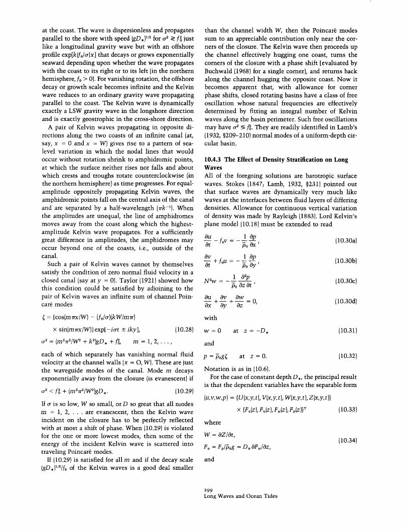
do show, however, characteristics of both short baro-clinic (figure 10.6) and long barotropic (figure 10.7)Rossby waves.

The oscillations having the two dispersion relations(10.23e) with D = D for first-class waves and (10.69)for second-class waves are mid-latitude plane-wave ap-proximations of solutions of LTE. Figure 10.8 plotsthe two dispersion relations together. A noteworthyfeature is the frequency interval between f and({/2f)(gD,) 2 within which no plane waves propagate.Taken at face value, this gap suggests that velocityspectra should show a valley between these two fre-quencies with a steep high-frequency [fo] wall and arather more gentle low-frequency [({/2fo)(gD,)12, n =0,1,2, .. .] wall. Such a gap is indeed commonly ob-served; but the dynamics of the low frequencies arealmost surely more complex than those of the linearp-plane. The latitude dependence implicit in the defi-nition of f and p is consistent with equatorial trappingof low-frequency first-class waves and high-frequencysecond-class waves. This is more easily seen in ap-proximations, such as the following, which better ac-knowledge the earth's sphericity.

)5

7

29

3

25 t

B9 a

'13

'25

37

49

51-300 -150 0 150 300km

Distance East of Centroal Site Mooring

Figure Io.6A Time-longitude plot of streamfunction inferredfrom objective maps of 1500-m currents along 28°N (centeredat 69°49'W) by Freeland, Rhines and Rossby (1975). There isevidence of westward propagation of phases. Currents at thisdepth are not dominated by "thermocline eddies" (section10.4.7) but are representative of the deep ocean.

10.4.5 The Equatorial ,8-PlaneFor constant depth D., the homogeneous LTE (10.5)may be equatorially approximated by expanding all var-iable coefficients in 8 and then neglecting 2,3, . . . .The resulting equatorial ,8-plane equations are

au doat YV= -g

av O~-t + fyu = -gt & y '

Ot ( eaux TY)= 0

(10.71a})

(10.71b)

(10.71c)

where x = a , y = a , and p = 2/a. They govern bothbarotropic and baroclinic motions provided that D, isinterpreted as the appropriate equivalent depth D, de-fined by (10.36)-(10.38). Moore and Philander (1977)and Philander (1978) give modem reviews.

Solutions of these equations can be good approxi-mations to solutions of LTE only when they decay veryrapidly away from the equator. But the qualitative na-ture of their solutions, bounded as y o, closelyresembles solutions of LTE bounded at the poles, even

81

93

105

117

129

141

153

165 S

177 ;-

189

201

213

225

237

249

261Okm

Distance North of Centrol Site Mooring

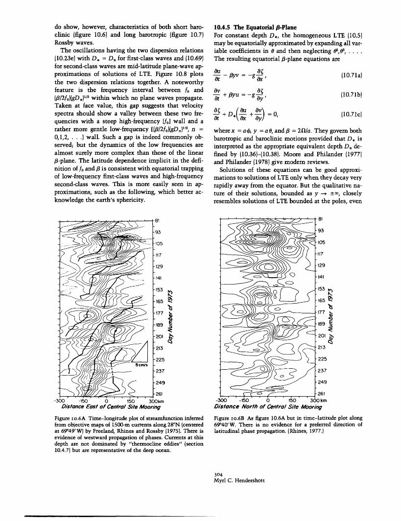
Figure o.6B As figure 10.6A but in time-latitude plot along69°40'W. There is no evidence for a preferred direction oflatitudinal phase propagation. (Rhines, 1977.)


20.. ' ATMOSPHERIC PRESSURE'' '''ATMOSPIERIC PRESSURE

MODE

BERMUDA

SEA LEV

BERMUDA

:, :~~~~~~~~~~~~~~~~~~~~~~~~~~~~~~~~~~~~~~~~~~~~~~~~~~~

' BOTTOM PRESSURE

I /,< BERMUDA S

AOML3

i;/'M E R T > ERD~~AOMLIMER~ REIKO

EDIE

.M.". .h .. ... li1...... ..... ...... .... i i lid

March MWy July

Figure 10.7 Time series of bottom pressure in MODE (Brownet al., 1975). The cluster of named gauges centered at 28°N,69°40'W show remarkable coherence despite 0 (180-km) sep-aration, and all are coherent with the (atmospheric pressurecorrected) sea level at Bermuda 650 km distant, labeled Ber-muda bottom). (Brown et al., 1975.)

\3,IlJ I

SUBSURFACE

when the equatorial approximation is transgressed.Historically these approximate solutions provided agreat deal of insight into the latitudinal variation ofsolutions of LTE.

Most of the solutions are obtainable from the singleequation that results when u,C are eliminated from(10.71). With

(10.72)v = V(y)exp(-iat + ix)

that equation is

,vy _ )-gD y2] V = 0.19y2 gD* ( D(10.73)

It also occurs in the quantum-mechanical treatment ofthe harmonic oscillator. Solutions are bounded asy -, +oo only if

( _ 12 1) = (2m + 1)( +g1) (gD) 11 2 I

m = 0, 1, 2,...,

and they are then

V(y) = Hm,.fl112/(gD ) 1/4] exp[-y 2 ,/2(gD )112],

(10.74)

(10.75)

wherein the H, are Hermite polynomials (Ho(i) = 1,H,(z) = z, ...).

The remaining solution may be taken to be v = 0with m = - 1 in (10.74). It is obtained by solving (10.71)with v = 0. The solution bounded as y -, _oo is

= exp[-iot + ilx - (8lIaby2/2]

-k

Figure IO.8 The f-plane dispersion relation

C"r = f + gD.12 + k2)

for first-class waves allows no waves with a2 < f. The 13-plane dispersion relation

a = -ll'2 + k + folgDj

for second-class waves allows no waves with a >(lf12f0o)gD.n)1 2.

(10.76)

with

I = o/(gD,) 12 (10.77)

[(10.77) is (10.74) with m = -1].The very important dispersion relation (10.74) with

im = -1, 0, 1, ... thus governs all the equatoriallytrapped solutions of (10.71). Introducing the dimen-sionless variables o, , , -1 defined by

o- = o(211A-114), 1 = Xla-'Al4),

Ix, y) = (, )(aA-114),

110.78)

t = [(2n)-'A1/4)

(A = 4 2a2/gD,) allows us to rewrite (10.73) and itssolutions (10.72), (10.75), (10.76) as

C2V + [(,2 - X2 - X/o) - 2]V = 0,

v = Hm,(7) exp(-ioT + iX: - 2/2),

(10.79)

(10.80)

= exp[-ior + i - (Xw/co)r/2], m = -1, (10.81)

while the dispersion relation (10.74) becomes


m�mrr

I

fo

.Dn) /2

1

wo2 - 2 - X/ow = 2m + 1, m =-1, 0, 1,.... (10.82)

These forms allow easy visualization of the solutionsand permit a concise graphical presentation of the dis-persion relation (figure 10.9).

The dispersion relation is cubic in or (or w) for givenvalues of 1 (or X) and m. For m > 1 the three rootscorrespond precisely to two oppositely traveling wavesof the first class plus a single westward-traveling waveof the second class. The case m = 0 (Yanai, or Rossby-gravity, wave) is of first class when traveling eastwardbut of second class when traveling westward. The casem = -1 is an equatorially trapped Kelvin wave, dy-namically identical to the coastally trapped Kelvinwave (10.27) in a uniformly rotating ocean.

The most useful aspect of these exact solutions istheir provision of a readily understandable dispersionrelation [(10.74) or (10.82)]. The latitudinal variation offlow variables is more readily discussed in terms ofWKB solutions of (10.73). One can easily see the salientfeature of the solutions, a transition from oscillatoryto exponentially decaying latitudinal variation as theturning latitudes YT of (10.73) (at which the coefficient[ ] of that equation vanishes), are crossed poleward. Forwaves of the first class, the term lfIro is small relativeto the other terms in the dispersion relation and in thecoefficient []. The corresponding turning latitudes yT)are therefore approximately given by

[y ]2 = (/0)2[l - 12 (gD*)/Cr2 ] I< (l3)2 (10.83)

For waves of the second class, the term r2/gD is smallrelative to the other terms in the dispersion relationand in the coefficient []. The corresponding turninglatitudes yT2 are therefore approximately given by

[Y(2)]2 = (gD*/lf 2)(-12 - 1(/cr) < gD*/4o 2 . (10.84)

Increasingly low-frequency waves of the first class andincreasingly high-frequency waves of the second classare thus trapped increasingly close to the equator.

Only first-class waves having frequency greater thanthe inertial frequency fy penetrate poleward of latitudey [by (10.83)]. Only second-class waves having fre-quency below the cutoff frequency (gD/4y2)112 pene-trate poleward of latitude y [by (10.84)]. This frequency-dependent latitudinal trapping corresponds to the mid-latitude frequency gap between first- and second-classwaves discussed in the previous section and illustratedin figure 10.8. The correspondence correctly suggeststhat trapping and associated behavior characterizeslowly varying in the WKB sense) packets of wavespropagating over the sphere as well as the globallystanding patterns corresponding to the Hermite solu-tions (10.75). Waves thus need not be globally coherentto exhibit trapping and the features associated with it.

Near the trapping latitudes, (10.73) becomes

O2V+ (-23 2 yTgDJ(y - yT)V = 0.

y 2 (10.85)

The change of variable = (2 f 2yT/gD*)113(y - YT) re-duces this to Airy's equation

a2V _ -V = 0, (10.86)

whose solution Ai(l) bounded as -* ox is plotted in( figure 10.10. This solution has two important features:

s (1) gentle amplification (like -vf"4) of the solution asthe turning latitude (* = 0) is approached from the

* equator; and (2) transition from oscillatory to exponen-tially decaying behavior in a region Ar) of order roughly

. ~ unit width surrounding the turning latitude. Conse-quently the interval Ay over which the solution of(10.85) changes from oscillatory to exponential behav-ior is Ay = [2, 2yT/gD * -113 A'v or, since ( = 2l/a andA0 = 1,

Figure Io.9 The equatorial (-plane dispersion relation (10.82)

J2 - 2 _ X / = 2m + 1.

Dimensional wavelengths and frequencies are obtained fromthe scaling (10.78) and are given for the barotropic mode (Do =4000 m, A = 20) and for the first baroclinic mode (Do = 0.1m, A = 106). For all curves but m = 0, intersections withdotted curve are zeros of group velocity.

Ay = a(Aro/2f1)-13

= a(2-' 2A -12or/2 )1/3

(10.87)

(10.88)

for maximally penetrating first- and second-classwaves. For diurnal ( = fl) first-class barotropic (A =20) waves, Ay 0.5a; for diurnal first-class baroclinic(A 106) waves, Ay = 0.013a. For 10-day (o = 0.1)second-class barotropic waves, y 0.25a. For 1-month


baroclinicwavelength

barotropicwavelength

6)

k,a,

I-10o-

0.25

0.13n

0. 67a

__ __.___..____ __ ___ _ ·̂ _

Figure Io.Io The Airy function Ai.

niques for dealing with the spherical problem now exist(section 10.4.8).

10.4.6 Barotropic Waves over Bottom ReliefStokes (1846; Lamb, 1932, §260) had shown that shoal-ing relief results in the trapping of an edge wave whoseamplitude decays exponentially away from the coast,but the motion was not thought to be important.

Eckart (1951) solved the shallow-water equations[(10.18) with fo = 0] with the relief D = ax. Solutionsof the form

= hx)exp(-iot + iky)

are governed by

a2 h Ohx + + [/(ag) - xk2]h = 0.

a ax

(10.89)

,10.90)

(or - .0311) second-class baroclinic waves, Ay = 0.03a.We thus obtain the important result that barotropicmodes are not noticeably trapped (Ay is a fair fractionof the earth's radius and the Airy solution is only qual-itatively correct anyway) but baroclinic modes areabruptly trapped (y is a few percentage points of theearth's radius).

The abrupt trapping of baroclinic waves at their in-ertial latitudes means that the Airy functions may de-scribe quite accurately the latitude variation of near-inertial motions. Munk and Phillips (1968) and Munk(chapter 9) discuss the structure.

The clearest observations of equatorial trapping areby Wunsch and Gill (1976), from whose paper figure10.11 is taken. Longer-period fluctuations at and nearthe equator have been observed, but their relation tothe trapped solutions is not yet clear.

When an equatorially trapped westward-propagatingwave meets a north-south western boundary (at, say,x = 0) it is reflected as a superposition of finite numbersof eastward-propagating waves including the Kelvin(m = -1) and Yanai (m = 0) waves (Moore and Philan-der, 1977). But when an equatorially trapped eastward-propagating wave meets a north-south eastern bound-ary, some of the incident energy is scattered into a pole-ward-propagating coastal Kelvin wave (10.29) and thusescapes the equatorial region (Moore, 1968). In latitu-dinally bounded basins, the requirement that solutionsdecay exponentially away from the equator is replacedby the vanishing of normal velocity at the boundaries.Modes closely confined to the equator will not begreatly altered by such boundaries; modes that haveappreciable extraequatorial amplitude will behave likethe -plane solutions of sections 10.4.1-10.4.4 near theboundaries. A theory of free oscillations in idealizedbasins on the equatorial ,8-plane could be constructedon the basis of such observations, but powerful tech-

Solutions of this are bounded as x - oo only if

c2 =k(2n + l)ag, n = 0, 1,...,

and they are then

h(x) = L,(2kx) exp(-kx),

(10.91)

(10.92)

where the L are Laguerre polynomials [L(z) = 1,L,(z) = z - 1, . . .]. The n = 0 mode corresponds toStokes's (1846) edge wave.

Eckart's solutions are LSW gravity waves refractivelytrapped near the coast by the offshore increase in shal-low water wave speed (gax)12. The Laguerre solutions(10.92) are correspondingly trigonometric shoreward ofthe turning points XT at which the coefficient [] of(10.90) vanishes, and decay exponentially seaward.

Eckart's use of the LSW equations is not entirelyself-consistent, since D = ax increases without limit.Ursell (1952) removed the shallow-water approxima-tion by completely solving

2 + 2 - k 24} = 00z 2 Ox2 (10.93)

subject to

= (or2/g at z = OOz

(10.94)

and

= 0 at z =-axd&9

(10.95)

plus boundedness of the velocity field (0l/Ox, ik,Od/Oz) as x - oc. He found (1) a finite number of coast-ally trapped modes with dispersion relation

o2 = kgsin[(2n + 1) tan-'a],(10.96)

n = 0, 1, . . . < [vr/l4tan-'a)- '2]


Ma.U

1-

E

U)z0

aoMJWzW

SOUTH

(10.11A) LATI

0

E

U)I.zc0

SOUTH

(10.11B) LAT

Q.U

IN",

I.-nzo

zw

SOUTH

(10.11C) LAT

Figure ro.II Energy at periods of 5.6d, m = 1 (A); 4.0d, m =2 (B); 3.0d, m = 4 (C); in tropical Pacific sea-level records asa function of latitude. A constant (labeled BACKGROUND)representing the background continuum has been subtracted

NORTH

TUDE (DEGREES)

NORTH

ITUDE (DEGREES)

NORTH

'ITUDE (DEGREES)

from each value. Error bars are one standard deviation of x2.The solid curves are the theoretical latitudinal structure fromthe equatorial 8/3-plane. (Wunsch and Gill, 1976.)


corresponding, for low n, to Eckart's results, plus (2) acontinuum of solutions corresponding to the coastalreflection of deep-water waves incident from x = oo andcorrespondingly not coastally trapped. Far from thecoast, the continuum solutions have the form =cos(/x + phase) exp[-iat + iky + (12 + k2)112z] and theirdispersion relation must require o2 2 gk. They arefiltered out by the shallow-water approximation. Figure10.12 compares Eckart's (1951) and Ursell's 1952) dis-persion relations.

With rotation fo restored to (10.18), (10.90) becomes(Reid, 1958)

02h Oh +[(o2 -f fk k -k2]x- + _x+[(oa-go _f) _ Ixk~]h = 0. (10.97)

Solutions still have the form (10.89), (10.92) but nowthe dispersion relation is

cr2 - f - fokaglo = k(2n + )ag, (10.98)

which is cubic in a-, whereas with fo = 0 it was quad-ratic. Rotation has evidently introduced a new class ofmotion.

That this should be so is clear from the fl-planevorticity equation [obtained by cross-differentiating(10.30a,b) and with afolOy = 3]:

a (v u fo a fo D fv o IDdt x dy D t D x r D y

n=4n=3

n=2

n=l

n=O

-2 -1 ' '1 '2

Figure o.I2A Eckart's (1951) dispersion relation (10.91)

S2 = K(2n + 1)

for the shallow-water waves over a semi-infinite uniformlysloping, nonrotating beach. For convenience in plotting, s =aef and K = gak/ even though problem is not rotating.

S

n=3n=2n=l

n=O

-2 -1 0 1 2

=0. (10.99)

We have already seen (section 10.4.4) that the term 3vgives rise to short and long Rossby waves (with thevortex-stretching term folD dO/Ot important only for thelatter) when the depth is constant. But in (10.99), thetopographic vortex-stretching term ufo/DVD plays arole entirely equivalent to that of fv = u-Vfo. Hence,we expect it to give rise to second-class waves, bothshort and long, even if / = 0. Such waves are calledtopographic Rossby waves. Over the linear beachD = -ax they are all refractively trapped near thecoast.

The nondimensionalization

Figure Io.12B Ursell's (1952) dispersion relation (10.96)

S2 = Ka-' sin[(2n + 1)tan-' a]

for edge waves, and the continuum

S2 > Ka-'

of deep-water reflected waves. For convenience in plotting, sand K are defined as above. Plot is for a = 0.2.

(10.100)

(10.101)

which is remarkably similar to (10.82) and plotted infigure 10.13.

The linear beach D = ax is most unreal in that thereis no deep sea of finite depth in which LSW planewaves can propagate. When the relief is modified to

(10.102)


s = a/f, K = kaglf2

casts the dispersion relation into the form

S3 -s[1 + (2n + 1)K] -K = 0,

= ax, 0 < x < Doa-1 (shelf)

Do, Doa - 1 <x < oo (sea),

_ _ __A~~~~~~

Figure Io.I3 The dispersion relation 10.91) for edge andquasi-geostrophic shallow-water waves over a semi-infiniteuniformly sloping beach. The dashed curves are the Stokessolution without rotation [(10.91) with n = 0]. Axes are as infigure 10.12. (LeBlond and Mysak, 1977.)

the most important alteration of the dispersion relationis an "opening up" of the long-wavelength part of thedispersion relation to include a continuum analogousto that of Ursell (1952) but now consisting of LSW first-class waves incident from the deep sea and reflectedback into it by the coast and shelf. These waves arenot coastally trapped. They are often called leakymodes because they can radiate energy that is initiallyon the shelf out into the deep sea. There are no second-class counterparts because the deep sea with constantdepth and 3 = 0 cannot support second-class waves.

The dispersion relation corresponding to (10.102) isplotted in figure 10.14. All of Eckart's modes are mod-ified so that cr2 > f2 save one (n = 0, traveling with thecoast to its right), which persists as cr -- 0 and is aKelvin-like mode. The others cease to be refractivelytrapped at superinertial (>fo) individual cutoff frequen-cies bordering the continuum of leaky modes. At sub-inertial frequencies there is an infinite family of re-fractively trapped topographic Rossby waves, alltraveling with the coast to their right (like the Kelvinmode) and all tending toward the constant frequencys = -1/(2n + 1) at small wavelengths. This dispersionrelation is qualitatively correct for most other shelf

shapes. It differs from its equatorial p-plane counter-part (10.82) only in the absence of a mixed Rossby-gravity (Yanai) mode and in the tendency of short sec-ond-class modes to approach constant frequencies.

Topographic vortex stretching plus refraction of bothfirst- and second-class waves are effective over anyrelief. Thus islands with beaches, submerged plateaus,and seamounts can in principal trap both first- andsecond-class barotropic waves (although these topo-graphic features may have to be unrealistically largefor their circumference to span one or more wave-lengths of a trapped first-class wave). A submarine es-carpment can trap second-class waves (then called dou-ble Kelvin waves; Longuet-Higgins, 1968b). Examplesof such solutions are summarized by Longuet-Higgins(1969b) and by Rhines (1969b).

First-class waves trapped over the Southern Califor-nia continental shelf have been clearly observed byMunk, Snodgrass, and Gilbert (1964), who computedthe dispersion relation for the actual shelf profile andfound (figure 10.15) sea-level variation to be closelyconfined to the dispersion curves thus predicted forperiods of order of an hour or less. Both first- andsecond-class coastally trapped waves may be variouslysignificant in coastal tides [Munk, Snodgrass, andWimbush (1970) and section 10.5.2]. At longer periods,a number of observers claim to have detected coastallytrapped second-class modes (Leblond and Mysak, 1977).A typical set of observations is shown in figure 10.16,after R. L. Smith (1978).

10.4.7 Long Waves over Relief with Rotation andStratificationThe two mechanisms of refraction and vortex stretch-ing that govern the behavior of long waves propagatingin homogeneous rotating fluid over bottom relief aresufficiently well understood that qualitatively correctdispersion relations may be found intuitively for quitecomplex relief even though their quantitative con-struction might be very involved. Stratification com-plicates the picture greatly. In this section, emphasisis upon problems with stratification that may be solvedwith sufficient completeness that they augment ourintuition.

By appealing to the quasi-geostrophic approximation,Rhines (1975; 1977) has given a far-reaching treatmentof the interplay between beta, weak bottom slope, andstratification for second-class waves. If equations(10.30a) and (10.30b) are cross-differentiated to elimi-nate pressure, and continuity (10.30d) is then invoked,the result is

(V a do) + fv w 0

in the 13-plane approximation (section 10.4.4) f = f,p = Of/ly. Now this equation is recast as an approxi-

3IoMyrl C. Hendershott

_ .___ . ___ �_�

and is linearized about z = -Do for sufficiently smalla.

With no bottom slope, solutions of (10.103)-(10.105)are

P = cos(Az) exp(-iort + ilx + iky),

= -1/ 2 + k2 + X2f2IoN2o),

with A given by (10.105) as a solution of

sin(XD0 ) = 0

i.e.,

X = nr/Do, n = 0, 1, 2,....

(10.106)

(l0.107)

(10.108)

(10.109)

These correspond to the barotropic (n = 0) and baro-clinic (n = 1, 2,...) Rossby waves of section 10.4.4.

With no beta but with bottom slope, solutions of(10.103)-(10.105) are

0 1 2 3 4 5i i I ~~~~~~~~~~~~~~~~~~~~~~~~~~~~~~~~~~~Ii

-0.5

-1.0 o

Figure IO.I4 The dispersion relation (solid lines) for edge andquasi-geostrophic shallow-water waves over a uniformly slop-ing beach (slope a = 2 x 10-3) terminating in a flat ocean floorat a depth of D = 5000 m. The dotted lines are for the semi-infinite uniformly sloping beach. The shaded region is thecontinuum of leaky modes. Axes are as in figure 10.12. (Le-blond and Mysak, 1977.)

mate equation in p by using (10.30c) plus thegeostrophic approximation to obtain

- 'p2p 0a2

9P 2 f p O ap = )0. (10.103)at X2 + zy2 + f x = -.

This result emerges from a more systematic treatment(Pedlosky, 1964a) as the linearized quasi-geostrophicapproximation. It is here specialized to the case ofconstant buoyancy frequency No. The free surface maybe idealized as rigid without loss of generality; thecorresponding condition on p is

dp = 0 at z =0. (10.104)az

The inviscid bottom boundary condition w = av at thenorth-south sloping bottom z = -Do + ay becomes,in quasi-geostrophic approximation,

d2P N x Op- Op +a--- =0 at z = -D, (10.105)

at Oz fo ax

P = cosh(Xz) exp(-iot + ilx + iky),

x = (No/fo)(12 + k2 )112,

alN2 coth (XD0 )

(10.110)

(10.111)

(10.112)

If ADO << 1, p is virtually depth independent and thedispersion relation (10.112) becomes

O = D-afol l(12 + k2 ). (10.113)

This is a barotropic topographic Rossby wave with vor-tex stretching over the relief playing the role of beta.If ADO >> 1, p decays rapidly away from the bottomand the dispersion relation (10.112) becomes

= Noll(l12 + k 2 )1 12 . (10.114)

Such bottom-trapped motions are of theoretical im-portance because they allow mid-latitude quasi-geo-strophic vertical shear and density perturbations at pe-riods much shorter than the very long ones predictedby the flat-bottom baroclinic solutions (10.106)-(10.109). Rhines (1970) generalizes this bottom-trappedsolution to relief of finite slope and points out that itreduces to the usual baroclinic Kelvin wave at a ver-tical boundary. Figure 10.17 shows what appear to bemotions of this type.

With both beta and bottom slope, solutions of(10.103) and (10.104) are

P = os (hz) exp( -irt + ilx + iky)cosh

r = -ll/(12 + k2 AX2f2IN2),

with A given by (10.105) as

aN 1X tan(AD0) = aNo

(10.1159)

(10.116g)

(10.1 17a)


M 2 _

/ -

,o

i ! i i i

2

Q

CD

CD

0 0.2 0.4 0.6

Cycles per kilometre

Figure IO.I5 Comparison of theoretical and observed disper-sion for the California continental shelf. Heavy lines O-IVcorrespond to theoretical dispersion relations for the first fivetrapped first-class modes. The dashed line bounds the contin-uum of leaky modes. The observed normalized two-dimen-sional cospectrum of bottom pressure is contoured for valuesof 0.03, 0.05, 0.10, 0.25, 0.50, 0.75, and 0.90 with the areaabove 0.05 shaded. (Munk, Snodgrass, and Gilbert, 1964.)

3I2Myrl C. Hendershott

__ _�____�_____ ___ �___

CAL LAOWIND

SAN JUAN'iWIND

15

f--\ \ rr,\ A r_ A1 \N-' V

JUN J RUG1976

'1'L ' L ..... AA -1 ml 1 M a-I

1 GJUN UL Ur

\&\t~,f',ln -\\ / if V

Figure Io.I6 Low-passed wind vectors and sea-level recordsfrom Callao (12°04' S and San Juan (15°20' S), Peru, and currentvectors from Y (80 m below surface off Callao) and from M

for case (a) and

X tanh(XD) = aN° ] (10.117b)

for case (b). Equation (10.117b) has one root X corre-sponding to a bottom-trapped wave for large a and toa barotropic B-wave for vanishing a. For vanishing a,(10.117a) reproduces the familiar flat-bottom baro-tropic and low-frequency baroclinic modes X = nrr/Do,n = 0, 1,.... When a is large the baroclinic roots areshifted toward X - (r/2 + n7r)IDo, so that the pressure(10.115a) and hence the horizontal velocity have a nodeat the bottom. There is thus a tendency for relief toresult in the concentration of low-frequency baroclinicenergy away from the bottom. With more realisticstratification this concentration is increasingly in theupper ocean. Rhines (1977) therefore calls such mo-tions "thermocline eddies" and suggests that they arerelevant to the interpretation of the observations offigure 10.18. It is straightforward to allow for an arbi-

(84 m below surface off San Juan). Sea level and currents showpropagation of events along the coast; wind records do not.(R. L. Smith, 1978.)

trary direction of the bottom slope, but the results arenot easy to summarize. Rhines (1970) gives a completediscussion.

A powerful treatment of second-class motion in arotating stratified fluid over the linear beach D = axhas been provided by Ou (1979), Ou (1980), and Ouand Beardsley (1980). They have generously permit-ted me to make use of their results in this discussion.Neglecting free surface displacement (so that w = 0 atz = 0) and eliminating u,v,w from (10.30) in favor of pyields

02p N 2 { 2p + p + P0-c \O +.yy~/=0,GZ2 -2 -OX d -

P =0 at z = 0,az

(i - +ior f - 0z2 ax y) N2o a

at z = -ax

(10.118)

(10.119)

(10.120)


a-Ic-JN

-10

15

-10

_

.

t

. ./.

I

4911 EU

-2

-4

20

4912 0 - "vlr l l\\ =

-20

4913 o ,

-20

04914

-20L

02AUG

01SEP

01OCT

Figure Io.I7A Currents at 39°10'N, 70°W (site D) at 205,1019, 2030, and 2550 m. The total depth is 2650 m. A "ther-mocline" eddy initially dominates the upper flow.

05 04 04 03 02 02MAY JUN JUL AUG SEP OCT

'73

Figure Io.I7B A high-passed version of figure 10.17A. Thelower layers are now dominated by fast-bottom intensifiedoscillations. (Rhines, 1977.)


20 04MAR APR

04MAY

03JUN

03JUL'73

20

10

U i /AAL\ y 11\

-10

4911 \Eo

4912

4913 '-E

4914

26 05MAR APR

u 1 7�- lK . _CI

· rrlr-·rln·r··r·r···rrrrrrr·rr·r·rrrl.·

1 I

I

ii

4

2

/_ - ///-\I/ \I

'M-cv

0 100 200 kmi . ,

a' is real and all of Ursell's (1952) results are im m edi-ately available. There are thus coastally trapped waveswhose dispersion relation is

o = f0 a'/{(l + a'2)1 12 sin[2n + l)tan-la']}

16

82 dyn cm

(10.127)

as well as a continuum of bottom-trapped waves thathave the form

P = cos(lx' + phase) exp[-iart + iky - (12 + k2 )112Z']

as x' X and that have their dispersion relation in-cluded in

(r = -Nsin(tan-a ) [(12 + k2)12 (10.128)

Figure Io.I8 Time-longitude plot of 501-1500-db dynamicheight along 28'N from MODE showing westward propaga-tion of "thermocline eddies" but at a rate significantly slowerthan that observed in 1500-m currents (figure 10.6). (Rhines,1977.)

The latter are just the bottom-trapped waves (10.110)-(10.112) of Rhines (1970).

Equation (10.128) is their dispersion relation in ahalf-plane bounded by the sloping bottom (Rhines,1970). The frequency may be either sub- or super-inertial. The coastally trapped waves have o >N sin(tan - a) [by analogy with the fact that for Ursell's(1952) edge waves oa2 < gk] and there are a finite num-ber of them:

n = 1,2,... < [r/(4tan-'a') - 1/2]. (10.129)

as the boundary-value problem governing periodic[exp(-it)] second-class and low-frequency first-classinternal) waves over the linear beach. Ou (1979) sawthat the affine transformation

z =3 f2 - r2)l12//No (10.121)

followed by a rotation of coordinates from (x,y,2) to(x', y, z') such that the beach z = -ax now becomesz' = 0 leads to

aop a¥P+ - k 2p = 0, (10.122)oz' O x12

Op kfO a'

On r (1 +a'2)1/2Pat z' = 0,

Op = 0 at z' = a'x' (10.124)On

for motions periodic in y[exp(ky)], and furthermorethat this is exactly Ursell's (1952) problem just turnedupside down; (10.122), (10.123), and (10.124) correspondto (10.93), (10.94), and (10.97). The transformed beachslope a' is given by

a' = aN(f2o - r2)-'/2. (10.125)

For second-class waves

o < f, (10.126)

Note that n = 0 would imply or = f but this does notsolve the full equations (10.30) and associated boundaryconditions.

In the limit of decreasing slope a', (10.129) allowsever more modes, and the dispersion relation (10.127)for coastally trapped waves simplifies to

a- = -fo(2n + 1). (10.130)

This is the low-frequency, short-wavelength second-class limit of the barotropic dispersion relation (10.98).We thus identify Ou's coastally trapped modes as thestratified analog of the already familiar refractivelytrapped second-class topographic Rossby waves.

Over the linear beach, then, stratification limits thenumber of second-class refractively trapped topo-graphic waves and opens up a new continuum of bot-tom-trapped waves. Figure 10.19 compares barotropicand baroclinic dispersion relations when the ocean sur-face is rigid. Further results are given by Ou (1979).

Suppose now that the linear beach terminates in aflat bottom of depth Do, as in (10.102). Ou's (1979)transformation allows us to deal efficiently with thestratified problem. Figure 10.20 summarizes theboundary-value problem and its alteration by Ou'stransformation into an equivalent problem in deep-water waves (figure 10.20D). In this latter problem, thedeep-water continuum that existed for the linear beachmust now be quantized into an infinite family of modesby repeated reflection between the shoaling and the

3I5Long Waves and Ocean Tides

DAY 01 -

125

t 149

173'

- 200 -100! !

Y

s

-0.3

-0.2

0.1

k

Figure Io.g9A The dispersion relation (10.130), viz., s =-1/(2n + 1) for topographic Rossby waves refractively trappedover the linear beach D = -ax beneath rotating homogeneousfluid. There are an infinite number n = 1,2,... of trappedmodes.

0.3

0.2

0.1

s=(N/fo) sin(tan-la)k

Figure Io.g9B The dispersion relation (10.127)

s = a'/{(l + a'2)"'2sin[(2n + 1)tan-la']},

where a' = aNol[fo(l-s2)"12], for topographic Rossby wavesrefractively trapped over the linear beach D = -ax beneathuniformly stratified (buoyancy frequency No) rotating fluid.There are a finite number n = 1,2,... < [r/( 4 tan-'a') - i] oftrapped modes all with frequencies s > Njal sin[tan- a]. Atlower frequencies a continuum of bottom-trapped modes re-flected from x = exists. Sketch is for No = 10fo, a = 10-2.

'\\ *I\

k

Figure Io.I9C Sketch of dispersion relation for topographicRossby waves in rotating stratified fluid over a linear beachthat terminates in a uniform-depth ocean. The continuum ofbottom-trapped modes that existed over the semi-infinitebeach is quantized. All dispersion curves pass through s = 0as k -- 0.

overhanging coasts. Low-mode edge waves have smallamplitude at the overhanging coast and are not muchaffected by it. But higher-mode edge waves have appre-ciable amplitude at the overhanging coast and theyblend smoothly into the infinite family of modes madeup of waves repeatedly reflected between beach andthe overhanging coast. All these results have directanalogs in the original stratified problem (figure10.20A). There are a number of second-class topo-graphic waves that are refractively trapped near thecoast and that have decayed to very small amplitudesat the seaward termination of the beach. The contin-uum of bottom-trapped waves present over the unend-ing linear beach is replaced by an infinite family ofbottom-trapped waves reflected repeatedly between thecoast and the seaward termination of the beach. In thespecial case a = of a perpendicular coast, their dis-persion relations are easily seen to be

oa = NDok/nrr (10.131)

and they then correspond to ordinary internal Kelvinwaves in this case there are no refractively trappedmodes). Other shelf geometries invite similar treat-ment. Figures 10.20E and 10.20F show the equivalentdeep-water wave problem for a step shelf. Deep-waterwaves on surface 1 of figure 10.20F that are shortenough that their particle displacements at the level ofsurface 2 are negligible correspond in the stratifiedproblem (figure 10.20E) to internal Kelvin wavestrapped against the coast. Deep-water waves on surface2 of figure 10.20F correspond to baroclinic counterpartsof the double Kelvin wave that, in homogeneous fluid,may be trapped along a discontinuity in depth (Lon-guet-Higgins, 1968b; see also section 10.4.6).

In general, if the equivalent deep-water wave prob-lem has the waveguide-like dispersion relationso2/g = F.(H,y,k), n = 1, 2, ... , with H,)y as defined infigure 10.20D, then the corresponding stratified shelfproblem must have the dispersion relation

kf a a'(1 = ) F.[((Da'la)2 + Doa-2 )"2

~r {1 + a'2) m'

tan- ' a', k] (10.132)

so that for all the dispersion curves oa - 0 as k - 0.The dispersion relation must thus qualitatively looklike figure 10.19C. Wang and Mooers (1976) have gen-eralized the problem numerically to more complexshelf profiles with nonuniform stratification N(z).

Ou's (1979) transformation is most useful for second-class motions (10.125) because for them the trans-formed coordinates are real. For first-class motionswith a-2 > f2 it still produces Laplace's equation butnow z' is imaginary. Wunsch (1969) has nonethelessbeen able to use it to discuss first-class internal wavesobliquely incident on the linear beach without rota-

3I6Myrl C. Hendershott

n=l

n=2n=3n=4etc.

n=l

n=2n=3n=n=b

-

x r v vr a r r^ F F he >

P,2 O 2

.,... . , + f -fo)} {p -kPz - 0

a{opx-fokp} +t(f 2-v?)/N

2pz - 0

(a)

q xP ' (kfo/)d/(l+a2 ) 1/2p

(c)

\ P2 0

x'

(b)

(d)

change, i.e., provided that the relief does not scatterenergy from one mode into others. Constancy of n isindeed a feature of Wunsch's solutions but it cannotbe expected to hold for more abrupt relief, especiallyif the relief slope exceeds the characteristic slope. Ifthe relief couples modes efficiently, then scatteringinto higher modes allows I to remain real even in deepwater far from shore so that energy is not refractivelytrapped near the coast. In principle, scattering into in-ternal modes thus even destroys the perfect trapping oflong surface gravity waves predicted by LSW theoryover a step shelf, but in practice appreciable trappingis often observed. The efficiency of mode coupling de-pends both on the relief and on the vertical profile N(z)of the buoyancy frequency, so that a general result forinternal waves is difficult to formulate.

(e) Stratified Problem

P1

(f)

Figure Io.2o The deep-water surface-wave analog (d,f) of twoshelf problems involving topographic Rossby waves in uni-formly stratified rotating fluid: (a) stratified problem; (b) resultof affine transformation; (c) result of rotation; (d) equivalentdeep-water problem (velocity potential ); (e) stratified prob-lem; (f) equivalent deep-water problem (atmospheric pressureP, must be maintained lower than P2 for physical realizabil-ity).

tion. This is the stratified analog of Eckart's (1951)nonrotating LSW study of waves over a sloping beach(section 10.4.6).

For beach slopes much smaller than the slope (or/N)of (low-frequency) internal wave characteristics (10.43),Wunsch thus found that internal waves are refractedjust like surface gravity waves by the shoaling reliefand that refractively trapped edge modes occur. Fromthe dispersion relation

o0) 2 (1 2 + k 2 )

for plane internal waves of the form

w = sin( D) exp(-i t + ilx + iky)

over a uniform bottom Do, I must ultimately becomeimaginary if Do is allowed to grow parametrically off-shore while n and k are held fixed. One would thereforeexpect a WKB treatment of internal waves over gentlyshoaling relief to result in refraction and refractivetrapping provided that the mode number n does not

10.4.8 Free Oscillations of Ocean BasinsFinding the free oscillations allowed by LTE in rotatingocean basins is difficult even in the f-plane (section10.4.2). Platzman (1975, 1978) has developed powerfulnumerical techniques for finding the natural frequen-cies and associated flow fields of free oscillations al-lowed by LTE in basins of realistic shape and bottomrelief. The general classification of free oscillations intofirst- and second-class modes characteristic of theidealized cases discussed in sections 10.4.2 and 10.4.5(effectively for a global basin) persists in Platzman's(1975) calculations. For a basin composed of Atlanticand Indian Oceans, there are 14 free oscillations withperiods between 10 and 25 hours. Some of these arevery close to the diurnal and semidiurnal tidal periods,and all of them, being within a few percentage pointsof equipartition of kinetic and potential energies, arefirst-class modes. There are also free oscillations ofmuch longer period, for which potential energy is onlyabout 10% or even less of kinetic energy; they aresecond-class modes.

I know of no extratidal peaks in open-ocean sea-levelrecords that correspond to these free oscillations. Thereis some evidence in tidal admittances for the excitationof free modes but the resonances are evidently not verysharp (see section 10.5.1). Munk, Bryan, and Zetler(private communication) have searched without suc-cess for the intertidal coherence of sea level across theAtlantic that the broad spatial scale of these modesimplies. The modes are evidently very highly damped.

10.5 The Ocean Surface Tide

10.5.1 Why Ocean Tides Are of Scientific InterestThe physical motivation for studying and augmentingthe global ensemble of ocean-tide records has expandedenormously since Laplace's time. In this section I havetried to sketch the motivating ideas without getting


,x

a-upx-rop ' t (fO-O-)/N- } '

io long waves ocean tides the main purpose of this · pdf filewaves and ocean tides around...

Documents