Preliminary and under revision Please do not quote without authors' permission

Investment and q with Fixed Costs: An Empirical Analysis

Andrew B. Abel and Janice C. Eberly*

This version 1999; Revised 2001

Abstract

Optimal investment depends both on expected returns and the costs of acquiring and installing capital. Empirical work using q-theory has emphasized the measurement of expected returns using Tobin's q, while more recent theoretical work focuses on investment costs, particularly fixed costs and irreversibility. This paper uses panel data to estimate a model of optimal investment and disinvestment using q to measure expected returns and allowing for a general "augmented adjustment cost function" -- incorporating fixed, linear, and convex adjustment costs. The results indicate both statistically and economically important nonlinearities, potentially arising from fixed costs, in the relationship between investment/disinvestment and its determinants. Our model suggests that investment and disinvestments should not be netted out empirically, and we find that disinvestment is non-negligible and behaves differently than positive investments. The nonlinearities we find imply that the cross-sectional distribution of q affects aggregate investment, so that the nonlinear model predicts annual aggregate investment substantially more successfully than does the linear model, particularly during large cyclical fluctuations.

* The Wharton School, University of Pennsylvania, and the N.B.E.R, Northwestern University and N.B.E.R. We thank Russell Cooper and seminar participants at the N.B.E.R. Summer Institute, Boston University, the Federal Reserve Banks of Boston and Cleveland, and Harvard University for helpful comments. We are grateful to the National Science Foundation for financial support and to Dale Jorgenson for making his data on capital taxes available to us. We also thank IBES for their data on analyst's earnings forecasts. This work was begun while Eberly was on the faculty of the Wharton School, and Eberly also thanks a Sloan Foundation Research Fellowship.

1

1. Introduction The empirical relationship between investment and q and has been investigated for twenty

years with varying degrees of success. The earliest empirical studies (e.g., Ciccolo (1975), von Furstenburg (1977)) built directly on Tobin's (1969) argument that investment is an increasing function of q, and these studies simply regressed aggregate investment on q, without explicitly specifying the functional link between investment and q. Around that time, Mussa (1977) showed that a version of the q theory can be derived rigorously from a model of investment by a firm facing convex costs of adjustment. The relationship between investment and q is a first-order condition equating the marginal cost of investment, including costs of adjustment, with the appropriate shadow price q. Thus, the estimated investment equations are estimates of the (inverse of the marginal) cost of adjustment function, taking account of purchase costs as well as convex adjustment costs.

Most of the attention over the last twenty years has focused on obtaining better measures of q. Capital income taxes were incorporated into empirical applications of the q theory by Abel (1980), Summers (1981) and Hayashi (1982). Hayashi also presented conditions under which the appropriate (but unobservable) shadow price of capital, sometimes known as marginal q, is identically equal to Tobin's q which is observable and is sometimes known as average q. This demonstration justified the use of securities market valuation of an entire firm for the purpose of assessing the marginal valuation of capital. Abel and Blanchard (1986) explored an alternative measure of q by forecasting future marginal revenue products of capital and future discount rates to estimate q as the expected present discounted value of profits accruing to a marginal unit of capital. These various extensions have all essentially taken as their starting point the equality of the marginal cost of investment and an appropriate measure of q. However, in the presence of fixed costs associated with investment, optimal investment does not always satisfy this first-order condition. For example, if the first-order condition is satisfied by a very small rate of investment, the net benefit to the firm of undertaking such a small rate of investment may not be large enough to overcome the fixed cost.

In a recent paper (Abel and Eberly (1994)), we have explored the theoretical implications of departures from the standard convex adjustment cost framework that underlies the q theory of investment. Even if the adjustment cost function is quadratic, which gives rise to a linear relationship between investment and q in the standard framework that does not include fixed costs, the introduction of fixed costs can introduce nonlinearities--indeed discontinuities--in the relationship between investment and q. In our earlier work we showed that taking account of fixed costs and allowing for a difference between the purchase and sale prices of capital, the optimal investment behavior of the firm can be characterized by potentially three regimes. For values of q above some upper threshold q

2, optimal investment is positive and an increasing

2

function of q. For values of q below some lower threshold q1, optimal investment is negative and

is an increasing function of q. For values of q between q1 and q

2 the optimal rate of investment is

zero, and this range is known as the range of inaction. We also showed that the values of these thresholds, q

1 and q

2, are completely determined by the augmented adjustment cost function

which takes account of the purchase and sale prices of capital, convex adjustment costs, and fixed costs. This finding leads us to focus our attention here on the characteristics of the augmented adjustment cost function.

In this paper we explore the empirical importance of the three regimes identified in our theoretical analysis. Two of the three regimes have nonpositive investment, and clear views of these regimes are obscured by aggregation across firms, across types of capital, and across time. Aggregating across firms to the level of the national economy, we always observe positive gross investment. Despite the fact that the two regimes with nonpositive gross investment are not clearly visible in aggregate investment data, these regimes may have important effects on the level of aggregate investment. Aggregate investment is comprised of the investment of individual firms (which themselves often represent aggregation across plants) which may more clearly display the two regimes of nonpositive investment. Hence we focus our analysis here on the investment of individual firms. Even at the level of firms in the Compustat data that we use, firms undertake some positive gross investment in every year. However, these firms frequently also display negative investment, i.e., they often sell capital even though they buy capital in the same year. The simultaneous purchase and sale of capital (our annual data, of course, aggregate across time, and so the purchase and sale of capital are not necessarily simultaneous) suggests that heterogeneity of capital is important and that firms engage in efforts to rearrange their holding of different types or vintages of capital. We will exploit this (unobserved) heterogeneity to estimate the threshold effects suggested by our more general formulation of augmented adjustment costs.

We find that such threshold effects are important; the data reject the exclusion of these effects at less than the 0.01 percent significance level in both manufacturing and non-manufacturing. Furthermore, the models allowing for a nonlinear relationship between investment and fundamentals produce far more accurate predictions of total investment than the linear model. The differences between the predictions of the different models are sometimes small, but the importance of the nonlinearities is most evident during three episodes: the 1981-82 recession, the subsequent recovery, and the 1990-91 recession. In the first two episodes, the linear model fails to take into account changes in the distribution of q that initially blunted the decline in investment and then led to a strong recovery in 1984. Following the 1990-91 recession, the nonlinear model and the data show investment rates recovering and an associated movement in the distribution of q; the linear model, by failing to account for distributional changes, shows no recovery at all.

3

While a large theoretical literature has emphasized the potential importance of fixed costs and irreversibility of investment,1 the empirical evidence is less extensive. Barnett and Sakellaris (1995) use the Compustat data to test whether the response of investment to Tobin's q depends on the level of q. They allow for three regimes and find (consistent with our results in Section 4.2) that the response of investment to Tobin's q is smaller in the high q regimes than in the low q regime. Doms and Dunne (1994), while not estimating a structural model, use the LRD database to examine investment of manufacturing plants. They find, for example, that more than half of all plants experience a year in which the capital stock rises by at least 37 percent. They characterize their data as evidence of "lumpy investment" at the plant level, and argue that this is consistent with models of nonconvex adjustment costs. Cooper, Haltiwanger, and Power (1995) use the same data to examine the implications of a model of machine replacement, focusing on the extensive investment margin and the age of equipment in place. Their data suggest that aggregate investment is largely determined by aggregate shocks affecting the number of plants investing, while the age distribution of equipment across these plants plays an important role subsequent to large movements in aggregate investment. Caballero, Engel, and Haltiwanger (1995) also use the LRD to estimate an "effective hazard function" relating investment to the gap between the plant's actual capital stock and an estimate of its desired capital stock. They find that the estimated effective hazard function is not flat, but increasing over some range of this gap, indicating that the investment response is nonlinear. Finally, in industry-level data, Caballero and Engel (1994) use two-digit manufacturing data on investment to estimate a model in which firms face stochastic fixed costs of investment. The dynamics evident in industry investment suggest that fixed costs are an important factor in the investment of the underlying firms, and therefore, that incorporating these costs improves the predictive ability of investment models.

Here, in addition to data on investment, we use data on disinvestment and the expected return to capital to estimate a structural model relating investment to its expected returns and costs -- allowing for a general formulation of the costs associated with changing a firm's capital stock. We begin in the next section by reviewing the theoretical model underlying our empirical specification of investment. In Section 3, we describe the data we use to estimate investment and disinvestment. Section 4 has four parts. In Sections 4.1 through 4.3, we report the results of estimating three different specifications of investment: a standard linear model, a nonlinear investment model with homogeneous capital, and a model with fixed costs and capital heterogeneity. Section 4.4 empirically characterizes disinvestment. We examine the aggregate

1 See for example, Pindyck (1988), Bertola and Caballero (1994), Dixit and Pindyck (1994), and Abel and Eberly (1995).

4

implications of our investment specifications in Section 5, and present concluding remarks in Section 6.

2. A Model of Optimal Investment We use the optimal investment policy derived in Abel and Eberly (1994) as the basis for

our empirical approach. In this section we show how optimal investment is related to q and the augmented adjustment cost function, allowing for fixed, linear, and convex adjustment costs.

The firm chooses its capital stock, K, to maximize the expected present value of operating profits, π(K,ε), less the cost of investing; the term ε in the operating profit function allows for stochastic shocks to the profit function2. The total cost of investing, c(I,K), depends on the level of investment, I, and the capital stock; it also depends on the price of capital, b, and a (vector) stochastic shock, ν, but we suppress dependence on these exogenous variables for the moment. This "augmented adjustment cost function" may have three components. First, there are costs proportional to investment, such as the price of the capital itself. This component of the augmented adjustment cost function is (piecewise) linear in investment, and potentially "kinked" at zero investment if the acquisition costs of capital differ from those associated with capital sales -- for example, if the purchase price of capital exceeds its resale price. Second, there are strictly convex costs of adjusting the capital stock, as in traditional q theory. Third, there may be a fixed cost of investing that is independent of the level of investment, though it may depend on the sign of investment. Specifically, the fixed cost of investment may differ from the fixed cost of disinvestment.

We define q as the marginal value to the firm of an additional unit of installed capital, i.e., q is the shadow price of installed capital. When the firm undertakes investment at rate I, the value of the firm increases by qI per unit of time, but the firm incurs a cost c(I,K) per unit of time. The optimal rate of investment I* maximizes the excess of qI over c(I,K), i.e.,

( )[ ]I qI c I K

I

* arg max ,= − (1)

For values of q that are sufficiently high (i.e., higher than a threshold value q2), I* is positive and

is an increasing function of q. For values of q that are sufficiently low (i.e., lower than a threshold value q

1), I* is negative and is an increasing function of q.3 For intermediate values of q, between

the thresholds q1 and q

2, the optimal value of investment, I*, equals zero. For nonzero values of

2Here, the capital stock, K, is a scalar. In section 4.3 we will introduce heterogeneity in the capital stock. 3If the threshold value q1 is nonpositive, then investment is irreversible.

5

I*, the optimal rate of investment is characterized by the first-order condition q = cI(I*,K), where

cI(I*,K) is the marginal cost of investment.4

For empirical implementation, let the augmented adjustment cost function take the following parametric form, now making explicit the dependence of costs on the price of capital, b

t, and the vector of cost shocks, ν

t:

c I K b a K b IIK

K

a K b IIK

K

t t t t t t t t t tt

tt

t t t t t tt

tt

( , , , ) ( )

( )

, ,

(1 )/

, ,

(1 )/

ν = + + + +

+ + + + +

+ + + + + ++

+

+ +

− − − − − −−

−

− +

+ +

− −

11

11

1 2

1 2

ν ν ββ

ν ν ββ

β β

β β

(2)

The "+" and "-" superscripts denote parameters that apply to positive and negative values of gross investment, respectively, the a parameters represent fixed costs, 1t is an indicator variable equal to one when investment is nonzero and zero otherwise, the b parameters represent the purchase and sale prices of capital, and the parameter β > 0 governs the curvature of the adjustment costs. The shocks to the augmented adjustment cost function may be of two types. The first, ν

1 , allows

a (potentially stochastic) shift in the linear component of adjustment costs, while the second, ν2, is

a multiplicative shock to the convex adjustment costs. Notice that the augmented adjustment cost function in equation (2) is linearly homogeneous in investment and the capital stock. Abel and Eberly (1994) show that with such a linearly homogeneous augmented adjustment cost function, and a linearly homogeneous operating profit function, the value of the firm is proportional to its capital stock so that Tobin's (average) q and marginal q are equal. In such a case, q can be measured by the ratio of the value of the firm to the replacement value of its capital stock.

Given the augmented adjustment cost function in equation (2), the optimal rate of investment is

( ) ( )[ ] ( )( ) ( )

( ) ( )[ ] ( )

IK

v q b v q q b v a

q b v a q q b v a

v b v q q q b v a

t

t

t t t t t t t

t t t t t

t t t t t t t

*, , ,

, ,

, , ,

, ,

, , , ,

, ,

=

− + >

− + − <

+ − + + + + +

− − − + + +

− − − − − − −

+ +

− −

2 1 2 1

1 1 2 1

2 1 1 1

0

β β

β β

if

if < <

if

(3)

According to equation (3) when the optimal rate of investment is nonzero, it is a constant elasticity function of the gap between q

t and the linear component of the augmented adjustment

4If there is a wedge between the purchase and sale prices of capital, then there will be some values of q for which no value of I* satisfies this equation. In this case, I* = 0.

6

cost bt + ν

1,t. The thresholds for investing and disinvesting, q

2(.) and q

1(.), may be stochastic, as

may be the response of nonzero investment to q. In the case of quadratic adjustment costs, β=1, and the relationship between investment and q is (piecewise) linear.

This general investment function potentially yields investment "episodes". When the expected returns to capital are high compared to its cost, the firm will invest at a rapid rate. When expected returns fall or costs rise sufficiently, then the firm ceases investing, and may eventually disinvest if returns fall or resale prices rise enough. If high expected returns and low costs are sustained, then high investment will be sustained as well -- generating an investment episode. As we will see below, this feature of our model is reflected in the firm-level data we consider, but is also evident in plant-level data. Using the LRD, Doms and Dunne (1994) find that the second-highest annual investment rate for each plant in their panel typically occurs in the year preceding or the year following the highest annual investment rate at that plant. Cooper, Haltiwanger, and Power (1995) also emphasize this serial correlation in investment by noting (in reference to Doms and Dunne) that "investment episodes are often spread across two (or sometimes three) years" (p.24). This feature is evident in their estimated hazard functions, which show that the highest probability of high investment occurs in the year following a high investment year; the probability subsequently declines, and then increases again.5

5 Cooper, Haltiwanger, and Power (1995) interpret the initially high probability of high investment as evidence of measurement error, in the form of an investment episode being spread over more than one calendar year. This also implies episodic investment at the monthly frequency, since investment is evidently spread over many months.

7

3. The Data and Characteristics of Investment and Disinvestment

We use annual data on publicly traded firms from the Compustat data base. The initial sample is an unbalanced panel of firms for the years 1974 to 1993. We eliminate observations in which the accounting identities governing capital accumulation are violated, or there is evidence of a merger or acquisition. The sample selection procedure is explained in more detail in the data appendix. The remaining sample contains 12075 firm-year observations. Tobin's (average) q is calculated as the value of equity plus debt less inventories, divided by the replacement value of the capital stock. The beginning-of-year equity value is used to obtain the market value of equity, and we construct the replacement value of physical capital using the method of Salinger and Summers (1983). We also constructed a tax-adjusted relative price of capital, p. The tax adjustment subtracts the investment tax credit in effect that year and the tax value of depreciation allowances from the implicit price deflator for capital goods. The relative price is then obtained by dividing this by a two-digit industry measure of the producer-price-index.6

We also utilize data from IBES on analysts' forecasts of earnings. These forecasts are available for a subset of firms in our sample since not all firms are followed by analysts and coverage does not begin until 198x. We use the IBES data on forecasted current year earnings and long-term growth.7 The "Long-Term Growth Forecast generally represents an expected annual increase in operating earnings over the next full business cycle. In general, these forecasts refer to a period of between three to five years."8 Concern about measurement error, particularly in the nonlinear estimation, led us to seek out the forecast data to use as instruments for q. Because of the forward-looking nature of the data, as well as its independent source and data collection method, we expected that the data would meet both criteria of a good instrumental variable: it is correlated with the independent variable, yet uncorrelated with the measurement error. When more than one analyst follows a company, we use the mean forecast.9

Table 1 presents summary statistics for the primary variables of interest. The fact that the mean exceeds the median for all variables (except the tax-adjusted price of capital, p) indicates the

6 In the manufacturing sector, a two-digit PPI is used as the denominator of the relative price of capital, and in the non-manufacturing sector, the PPI for finished goods is used in the denominator of the relative price of capital. 7 We also used data on subsequent year earnings, but later omitted it from the results. Since fewer observations are available on this variable, we found that it limited our sample size without substantially changing the results. 8 I/B/E/S glossary, page 23. 9 Using the median, rather than the mean, had virtually no effect on our results. Using the long-term growth forecast reduced our IBES sample size by more than 25%. We originally matched 2142 firm-years, but for only 1576 of these observations was the long-term growth forecast available. However, since we found that the long-term growth forecast was an excellent predictor of q, we reduced the size of the sub-sample in order to improve instrument quality.

8

positive skewness evident in these data. We examine this result in more detail, focusing on investment and disinvestment, in Table 2.

Table 1: Descriptive Statistics

CompuStat

Manufacturing N=5803

Non-manufacturing N=6272

mean median mean Median Capital, K (millions)

66 (151)

20 77 (153)

26

I+/K 0.15 (0.13)

0.12 0.16 (0.15)

0.12

I-/K 0.02 (0.08)

0.001 0.03 (0.09)

0.002

π/K 0.15 (0.28)

0.14 0.08 (0.22)

0.07

Tobin's q 1.29 (0.70)

0.97 1.23 (1.02)

0.91

tax-adjusted p 0.61 (0.08)

0.64 0.61 (0.07)

0.63

I/B/E/S Manufacturing N=881

Non-manufacturing N=695

Growth Forecast

17.2% (7.8%)

15.0% 18.3% (7.0%)

17.4%

Forecast Earnings/K

0.12 (0.20)

0.11 0.13 (0.17)

0.10

Standard deviations of the data are in parentheses. Dollar values are in 1987 dollars. Capital stock, K, is measured beginning-of-period. Operating profit, πt, is measured at the end of the previous period.

9

Table 2: Investment and Disinvestment Investment and Disinvestment

Manufacturing N=5803

Non-manufacturing N=6272

Rates: standard dev. skewness standard dev. skewness I+ /K 0.13 2.0 0.15 1.8 I- /K 0.08 21.4 0.09 12.3 Levels: mean median mean median I+ , given I+ >0 (millions)

8.5 (19.2)

1.9 13.1 (26.7)

2.7

I- , given I- >0 (millions)

1.2 (4.3)

0.12 2.8 (26.1)

0.28

Disinvestment Occurrence:

Share of observations:

Share of firms: Share of observations:

Share of firms:

Incidence of I->0 0.46 0.79 0.50 0.80 Standard deviations of the data are in parentheses. Dollar values are in 1987 dollars.

The first two rows of Table 2 report higher moments of the firms' investment and

disinvestment rates. The standard deviations are both high (as compared to the means), and the skewnesses of both investment and disinvestment are large and positive in both sectors.10 This positive skewness suggests that investment is temporally concentrated, and the serial correlation pattern confirms this tendency. In 47 percent of the manufacturing firms, the second highest annual rate of investment occurs in either the year immediately preceding or immediately following the year with the maximum investment rate. In non-manufacturing, the two highest annual investment rates occur consecutively in 50 percent of the firms.11 Consistent with the plant level data described in the previous section, these data suggest that investment is episodic: a given firm exhibits a few years of relatively high investment, and these years tend to occur consecutively.12 10 In both cases, the degree of skewness is comparable to that implied by a log-normal distribution with the first and second moments found in our data; the logs of both investment and (positive) disinvestment are slightly negatively skewed in both sectors. This degree of skewness is comparable to that found by Doms and Dunne (1994) for firms in their study of manufacturing plants. They compute the ratio of maximum annual investment to total investment over the sample period as a measure of temporal concentration. In our unbalanced panel, this statistic is less informative. In our data, the ratio of maximum annual investment to average annual investment is 2.5 in manufacturing and 2.6 in non-manufacturing. Care should be taken in interpreting even this statistic, however, since it is not independent of sample size. 11 While in a short time series it is more likely that the peak year of investment will be near the second-highest year of investment, values similar to those reported in the text are found in a subsample of firms for which all 20 years of data are available. In particular, in this subsample, the probability that the two highest investment rates will occur consecutively is 45 percent in manufacturing and 52 percent in non-manufacturing. 12 Serial correlation in investment rates is measured directly by noting that for a given firm in our sample, the correlation between current and lagged investment rates is 0.62 in manufacturing and 0.67 in non-manufacturing.

10

While disinvestment does not occur every period in every firm, it is however, not unusual. The last row of Table 2 indicates that about 80 percent of firms in both manufacturing and non-manufacturing sell capital in at least one year in the sample, and these years account for 46 percent of all observations in manufacturing and 50 percent in non-manufacturing. While many of these disinvestments are small (consistent with the skewness noted above), the mean annual disinvestment is $1.2 million in manufacturing, and more than twice that amount in non-manufacturing. The means are an order of magnitude larger than the medians in each sector. The incidence of investment is not tabulated in Table 2 because positive investment occurs in all of our valid observations. Again consistent with the temporal concentration finding, however, some investments are very small. The lowest annual level of investment recorded in the sample is $1000, undertaken by a small firm (its sales never exceed $1.5 million) in the electrical machinery industry. The 25th percentile of the investment rate (I/K) is 6 percent in manufacturing and 5 percent in non-manufacturing industries.

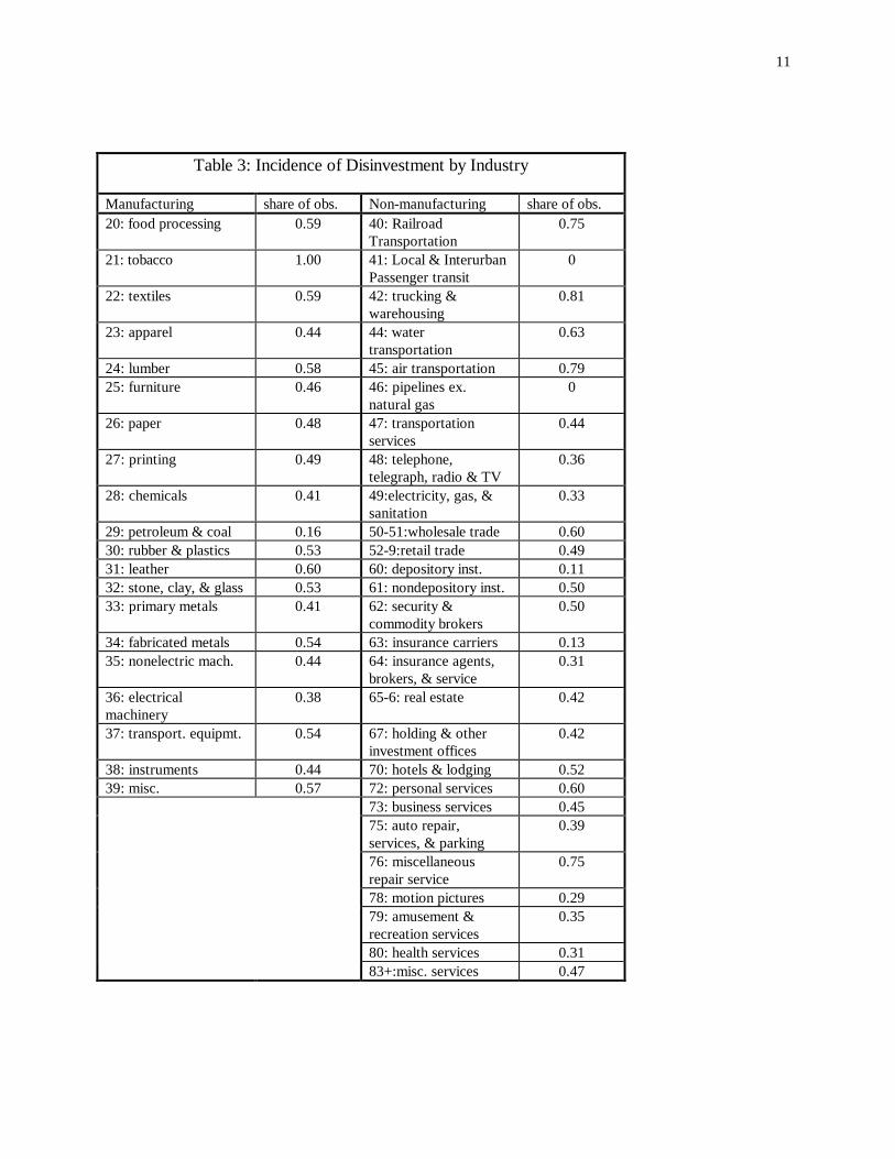
Interestingly, the incidence of disinvestment is not very concentrated by industry. Table 3 cross-tabulates two-digit industries and the incidence of disinvestment. In manufacturing, the incidence of nonzero disinvestment ranges from 16 percent of the observations (in Petroleum & Coal) to 100 percent (in Tobacco), while in non-manufacturing, the incidence of nonzero disinvestment ranges from 0 percent (in Local & Interurban Passenger Transit, and Pipelines except Natural Gas) to 81 percent (in Trucking & Warehousing).

11

Table 3: Incidence of Disinvestment by Industry

Manufacturing share of obs. Non-manufacturing share of obs. 20: food processing 0.59 40: Railroad

Transportation 0.75

21: tobacco 1.00 41: Local & Interurban Passenger transit

0

22: textiles 0.59 42: trucking & warehousing

0.81

23: apparel 0.44 44: water transportation

0.63

24: lumber 0.58 45: air transportation 0.79 25: furniture 0.46 46: pipelines ex.

natural gas 0

26: paper 0.48 47: transportation services

0.44

27: printing 0.49 48: telephone, telegraph, radio & TV

0.36

28: chemicals 0.41 49:electricity, gas, & sanitation

0.33

29: petroleum & coal 0.16 50-51:wholesale trade 0.60 30: rubber & plastics 0.53 52-9:retail trade 0.49 31: leather 0.60 60: depository inst. 0.11 32: stone, clay, & glass 0.53 61: nondepository inst. 0.50 33: primary metals 0.41 62: security &

commodity brokers 0.50

34: fabricated metals 0.54 63: insurance carriers 0.13 35: nonelectric mach. 0.44 64: insurance agents,

brokers, & service 0.31

36: electrical machinery

0.38 65-6: real estate 0.42

37: transport. equipmt. 0.54 67: holding & other investment offices

0.42

38: instruments 0.44 70: hotels & lodging 0.52 39: misc. 0.57 72: personal services 0.60 73: business services 0.45 75: auto repair,

services, & parking 0.39

76: miscellaneous repair service

0.75

78: motion pictures 0.29 79: amusement &

recreation services 0.35

80: health services 0.31 83+:misc. services 0.47

12

4. Estimation

The estimation results below are divided into four sections: the first three sections focus on investment, and the fourth section focuses on disinvestment. The first section presents and estimates a standard linear model of investment (β = 1) that allows comparison to the literature as well as comparison to subsequent nonlinear models. In the second section we relax the assumption that β = 1 and estimate a nonlinear investment equation based on convex adjustment costs that are not quadratic. In the third section we return to the assumption that β = 1, but allow for capital heterogeneity, which leads to a nonlinear relationship between investment of a firm and q. In the fourth section, we switch our attention to disinvestment behavior and estimate a threshold model of disinvestment. In each of the four sections, we first present the econometric specification derived from the general optimal investment and disinvestment policy of Section 2, followed by the estimation results.

4.1 The Linear Investment Specification The standard linear investment function relating investment to Tobin's q and the price of capital is derived under the assumption of quadratic adjustment costs (β = 1). Setting β = 1 in equation (3), assuming that capital is homogeneous and that there are no multiplicative shocks to the adjustment technology (ν

2 is constant), we obtain a linear relationship between investment and its

fundamental determinants. Since q is measured at the beginning of the period and investment occurs over the subsequent year, we allow for the possibility that news about the real interest rate becomes available to the firm subsequent to our measurement of average q. To a first approximation, the true value of an additional unit of capital, q*(t), is given by q*(t) = q(t) - q(t)[r(t)/r - 1], where q(t) is measured beginning-of-period average q, r(t) is the realized real interest rate during period t, and r is the real interest rate embedded in beginning-of-period average q. Thus, for a given value of beginning-of-period q(t), a higher realized real interest rate reduces the true return to investing.13 Using equation (3), the investment equation is therefore14

IK

q p ri t

i tv i t v i t t i t i t

,

,, , ,= − + + + +1

2 2α γ υ υ η . (4)

The true price of capital bi,t

is assumed to be proportional to the measured index, pi,t with factor

of proportionality, α (though we instrument to correct for classical measurement error). The 13 This formula is obtained by a first-order Taylor approximation to the true period t value of q around the beginning-of-period value, taking into account the period t real interest rate innovation. 14In sections 4.1, 4.2, and 4.3 we confine attention to positive investment and we dispense with the superscript "+". In section 4.4, which focuses on disinvestment, we dispense with the superscript "-".

13

parameter γ measures the response of investment to the real interest rate, which we compute as the annual return on 6-month commercial paper less year-over-year inflation in the producer price index.15 The linear cost shocks, ν

1,t, may have a firm-specific component, υ

i, and a year-specific

component, υt, and η

i,t is a mean-zero transformed error term also arising from unobserved

shocks to the price of capital. We estimate equation (4) using fixed-effects to remove the firm-specific component and

also by first-differencing, with very similar results. The fixed-effect regression is also estimated using a quantile (median) regression to demonstrate that our results are not sensitive to outliers in the data. We use instrumental variables estimation both because of concern about classical measurement error and also due to the possibility of "bubbles" on the value of the firm, which is the numerator of average q. Since fundamental q is the expected present value of marginal returns to capital, we use marginal returns as an instrument for q. With a linearly homogeneous operating profit function (as we assumed in Section 2), average and marginal returns are equal, so we use as instruments two lags of average operating profits, π/K.16 The instrument set includes one lag of the tax-adjusted price of capital, as well as time and two-digit industry dummy variables.

The results of the linear estimation in the manufacturing sector are presented in Table 4. They are largely similar to those found in the existing literature, though the coefficients on Tobin's q are slightly larger and more significant than found in some studies. The coefficients are generally robust to the different methods of removing the fixed effect, as well as to the "absolute deviation" criterion utilized by the quantile regression. The magnitude of adjustment costs implied by these coefficients range from 59 percent of total investment up to 545 percent.17 The coefficients on the tax-adjusted price of capital are all negative, and both statistically and economically significant in all of the estimation procedures. The real interest rate has a significant negative effect on investment in all of the specifications. When we allowed the nominal interest rate and the inflation rate to enter the regressions separately, we found however that most of this effect is due to inflation rather than to the nominal interest rate.

Table 5 presents the results of estimating the linear specification in the non-manufacturing sector. Again Tobin's q is statistically significant in all of the regressions. The magnitude of the 15 These values are found in Tables B72 and B67, respectively, of the Economic Report of the President, 1995. 16Note that the use of (lagged) π/K as an instrumental variable for q does not imply the presence of cash flow or liquidity effects; by using π/K as an instrument, it is allowed to affect investment only through its effect on q. This effect is present in a model without financing considerations. 17 These values are obtained by noting from equation (4) that the coefficient on Tobin's q is 1/v2 and noting from equation (3) that the total amount of adjustment costs is given by (v2/2)(I/K)2K. Letting ρdenote the estimated coefficient ( =1/v2), the ratio of total adjustment costs to investment I is (1/2)(1/ρ)(I/K). In light of the skewness in investment rates noted in Table 1, we evaluate (I/K) at its median, which is 0.12 for both manufacturing and non-manufacturing.

14

coefficients on Tobin's q imply a range of total adjustment costs from 46 percent of total investment I to 857 percent. The coefficient on the price of capital is in general statistically significant and less than zero. The real interest rate again has a negative effect on investment, though the effect is not statistically significant in the first-differenced specifications for non-manufacturing.

Table 4: Linear Regression Results Manufacturing

Regressors:

Procedure Tobin's q p r R2 Fixed-effects OLS

0.031 (0.002)

-0.26 (0.03)

-0.16 (0.06)

0.08 (within)

Fixed-effects IV

0.101 (0.006)

-0.25 (0.03)

-0.43 (0.06)

0.05 (within)

1st-difference OLS 0.011 -0.17 -0.18 0.02 (0.004) (0.06) (0.08) 1st-difference IV 0.060 -0.15 -0.25 0.01 (0.008) (0.05) (0.08) Fixed Effects, Quantile regression

0.030 (0.002)

-0.19 (0.02)

-0.14 (0.05)

0.04 (pseudo)

Fixed-effects OLS (IBES Sample)

Fixed-effects IV (IBES Instruments)

Standard errors are in parentheses and are calculated using the White (1980) heteroskedasticity-robust method. Coefficients on year dummies in the fixed effect regressions are not reported. The instrument set includes two lags of π/K, lagged p, the real interest rate and the year dummy variables.

15

Table 5: Linear Regression Results Non-manufacturing

Regressors:

Procedure Tobin's q p r R2 Fixed-effects OLS

0.041 (0.003)

-0.27 (0.03)

-0.34 (0.08)

0.08 (within)

Fixed-effects IV

0.130 (0.012)

-0.19 (0.04)

-0.52 (0.08)

0.05 (within)

1st-difference OLS 0.007 -0.18 -0.07 0.01 (0.004) (0.05) (0.09) 1st-difference IV 0.050 -0.16 -0.11 0.01 (0.010) (0.05) (0.09) Fixed Effects, Quantile regression

0.041 (0.002)

-0.24 (0.02)

-0.32 (0.06)

0.06 (pseudo)

Standard errors are in parentheses and are calculated using the White (1980) heteroskedasticity-robust method. Coefficients on year dummies in the fixed effect regressions are not reported. The instrument set includes two lags of π/K, lagged p, the real interest rate, and the year dummy variables.

16

4.2 Nonlinear Investment Estimation

Now we allow the investment function to be nonlinear by departing from the assumption that the adjustment costs are quadratic. Recall from equation (3) that when q is higher than the upper threshold q

2, a firm's investment is related to Tobin's q and the tax-adjusted price of capital

according to ( ) ( )IK

q bi t

i tt i t i t

,

,, , ,= − −

−ν ν

β β2 1 . Taking logs, substituting αp

i,t for b

i,t, inserting the

interest rate effect as in equation (4), and allowing the multiplicative cost shock ν2,t to have a

firm-specific component, υ i , and a year-specific component, υ t , as well as a log-normal stochastic component, we obtain

( )ln ln,

,, ,,

IK

q p ri t

i ti t t i t i ti t

= − + − + + +β α γ ν υ υ η1 . (5)

The term v1 is taken to be a constant in this specification. This equation is estimated using

nonlinear least squares, taking first-differences to eliminate the firm-specific effects. The results of estimating equation (5) are shown in Table 6. The price of capital again has a negative effect on investment in both manufacturing and non-manufacturing. Interestingly, the curvature parameter is significantly less than one (but significantly positive) in both sectors, suggesting a strongly concave relationship between investment and fundamentals. An F-test rejects the restriction β = 1 at less than 1 percent significance in both manufacturing and non-manufacturing. This result is consistent with Barnett and Sakellaris' (1995) finding of a decreasing response of investment rates to q for higher values of q, even though they use a different econometric approach and data sample than is employed here.

Table 6: Nonlinear Investment Specification

Method: NLLS

Manufacturing R2=0.013

Non-manufacturing R2=0.027

Parameter Coefficient Est. Std. Error Coefficient Est. Std. Error

curvature, β 0.25 (0.02) 0.37 (0.05) price, α 0.93 (0.49) 4.2 (1.33) interest rate, γ -0.01 (1.24) -2.8 (1.08) shock, ν

1 0.63 (0.34) 2.8 (0.95)

The table reports the results of estimating equation (5) in first-differences. The non-manufacturing estimation includes one-digit industry dummy variables.

17

4.3 Estimation with Capital Heterogeneity

In this section we again assume β = 1, but now we allow for heterogeneity in the types of capital purchased by firms. These capital types may differ in their values of q and the linear component of their adjustment costs.18 Indexing types of capital by n (distributed according to the cumulative distribution function F(n) on the support 0,n ), adjustment costs are assumed to

apply separately to each type of capital, so that total convex adjustment costs are of the form19 ν2

2

02IK

K dF nnn

∫ ( ) . We can then write optimal investment in capital of type n (suppressing firm

and time subscripts for now) as

( )IK

q b q q b ann n n n n= − − >1

21 2ν ν ν, , ( , , ) if (6)

Thus, for each type of capital, there is a type-specific investment threshold, which is a function of the type-specific component, ν1,n , of the linear adjustment costs. We do not observe the variation

across n in qn or v

1,n. To deal with the unobserved variation, we assume that q

n = q + ε

n and v

1,n

= v1 + η

n where E{ε

n} = E{η

n} = 0.20 Define ω ε ηn n n≡ − as a scalar that accounts for all

unobserved variation across types of capital in qn - b - v

1,n. Specifically, q

n - b - v

1,n = q - b - v

1 +

ωn. Substituting this expression for q

n - b - v

1,n into equation (6) yields

( )IK

q b q q b ann n= − − + >1

21 2ν ν ω ν if , ( , , ) (7)

The threshold q

2,n that induces investment in capital of type n is found by substituting

equation (7) into the optimality criterion in equation (1) and finding the value of q at which the optimal rate of investment becomes positive. This calculation yields 18 This heterogeneity in the linear component of costs may be due to price heterogeneity or to differences in the linear part of adjustment costs. This distinction is irrelevant for the rate of investment, but we return to it when calculating the level of augmented adjustment costs paid by the firm. It is also possible to allow for heterogeneity in the fixed cost across types of capital. 19 With heterogeneity in types of capital, we aggregate these types using their prices as weights, so that K should be interpreted as the total cost of the firm's capital stock. 20If the operating profit function and the augmented adjustment cost function are both homogeneous of degree one in the stocks and rates of investment of all types of capital, then the value of the firm V is a linearly homogeneous function of all types of capital. Integrating over all types of capital n, we have

qK V V K dF n q K dF nK n

n

n n

n

n≡ = ≡∫ ∫( ) ( )

0 0

. Therefore, ( )q q K K dF nn n

n

= ∫ / ( )0

so that observable average q for the

firm is a weighted average of the unobservable marginal q's specific to each type of capital.

18

q b an n2 1 22, .= + − +ν ω ν (8)

Because ω

n is unobserved and random across types of capital n, the thresholds q

2,n, are

unobserved and random across n. For types with low thresholds, investment will occur at low values of q, whereas the firm will not invest in "high threshold types" until q has reached a similarly high value.

The total investment of the firm is obtained by aggregating equation (7) over types of capital, n, remembering that investment in capital of type n is only nonzero if q

2,n < q. We can

think of ordering the types of capital according to the value of their thresholds, q2,n

, then integrating over investment until q

2,n = q. We therefore integrate investment using the density

function dF(q2,n

) of the thresholds and an upper limit of integration equal to the firm's current value of q. This calculation yields

( ) ( ) ( ) ( ) ( )

( ) ( )( )[ ] ( ) ( ) ( )

IK

q b dF q q b v F q dF q

F q q b q qF q

dF q

n

q

n n

q

n

n

q

n

= − − + = − − +

= − − + ≡

+∫ ∫

∫

1 1

1 1

21

02

21

02

21

02

νν ω

νω

ν ν ω

, ,

,, . where Ψ Ψ (9)

The standard linear investment specification is a special case of this function, with F(q) equal to one and Ψ (q) equal to zero. Taking logs of both sides of equation (9), allowing for the interest rate effect introduced in equation (4) and making explicit the firm and time subscripts, we obtain

( )[ ] ( )( )ln ln ln ,,

,, , , , ,

IK

F q q b r qi t

i ti t i t i t t i t i t i t

= + − + − + + + ++ γ ν υ υ η1 Ψ (10)

where we have allowed the multiplicative shock to adjustment costs, v

2,t, to have a firm-specific

component, υi , as well as a stochastic component which we assume is log-normally distributed -- so that ηi,t is normally distributed. We assume that the firm chooses the types of capital in which it will invest before observing the realization of v

2 , and after observing v

2 optimally chooses the

amount to invest in each type.21 Since v2 is common to all types of capital, this assumption is

21 Since the multiplicative shock, v

2 , and therefore, its stochastic component affects the investment threshold (see equation (8)), the distribution of the thresholds would be stochastic as well. If, as we assume, the firm chooses the extensive margin of investment before the realization of the stochastic term, the distribution F(q2,n) will not be time-varying.

19

similar to a putty-clay specification for the current period's investment: the firm first chooses the factor share of each type of capital and then chooses the scale of investment after observing the value of v

2.22

We now consider the form of the c.d.f. F(q2,n). In the estimation, we assume that ωn is

normally distributed.23 Under these assumptions, q2,n given in equation (8) is a normally distributed random variable across types of capital. Specifically,

( )q N b vn2 1

2, , is + + µ σ (11)

where { }µ ω ν≡ − +E an 2 2 (11b)

and { }σ ω ν222≡ − +var n a (11c)

Thus, the c.d.f. F(q) in equation (10) is cumulative normal, with mean ( )b v+ +1 µ and variance

σ2. We discuss the implications of other distribution functions when we present the results below.

In the estimation, we first-difference equation (10) to eliminate the firm fixed-effect, again allowing for the interest rate effect introduced in equation (4). The estimation equation is therefore

( )[ ] ( )( )∆ ∆ ∆ Ψ ∆ln ln | , , , ln ~ ,,

,, , , , , ,

IK

F q p r q p r qi t

i ti t i t t i t i t t i t t i t

= + − + − + + ++ α γ µ σ α γ ν υ η1 (12)

where ∆ represents the first-difference operator, and % ,ηi t is a transformed (still normally-

distributed) error term. We estimate the parameters µ and σ, and the coefficients α and γ on the relative price of capital and the interest rate, respectively. The estimation is implemented using non-linear least squares. The results of estimating equation (12) for the manufacturing and non-manufacturing sectors are presented in Table 7.24 22 Observe from equation (7) that the realization of v

2 has a proportionate effect on investment in each type of

capital. 23 More fundamentally, we assume that the deviations, εn, of qn from q and the relative price shocks, v1,n , are both normally distributed. These assumptions imply that ωn is normally distributed. It is also possible to have a distribution of fixed costs over n, where the fixed costs are distributed χ2 (1). In this case, the thresholds are still normally distributed and our analysis proceeds as below. This specification, however, requires additional assumptions in the calculation of augmented adjustment costs (since the distribution of fixed costs is then also unobserved) so we choose this simpler specification. 24 Although in this section we have assumed the curvature parameter, β, is one (so that adjustment costs are quadratic), we can test this restriction by estimating β as the coefficient on the term ( )( )ln , , ,q b qi t i t i t− − +ν1 Ψ in

20

For the manufacturing sector, the mean, µ, is positive and significantly greater than zero. The fact that the variance is significantly greater than zero indicates that the c.d.f. term is relevant in the estimation, since by driving the variance to zero, the c.d.f. would become simply a constant term. We consider the implications of the estimated magnitudes of µ and σ below. The coefficient α is significantly positive so the price of capital continues to have a significant negative effect on investment. The interest rate effect, measured by the coefficient γ is large and negative, but not statistically significant. The linear cost shock, ν

1, is significantly negative. We return to

the interpretation of this shock when we calculate adjustment costs below. In non-manufacturing the mean, µ, is again positive and significantly greater than zero. The variance is significant, and indicates the relevance of the c.d.f. term in non-manufacturing data, as well. The price effects continue to be negative and significant in this sector, while the interest rate effect is again negative but insignficant. An F-test rejects the exclusion of the c.d.f. term at less than the 0.01 percent significance level in both manufacturing and non-manufacturing.

Table 7: Investment with Capital and Threshold Heterogeneity

Manufacturing R2=.02

Non-manufacturing R2=.03

Coefficient Est. Std. Error Coefficient Est. Std. Error

mean, µ 7.10 (0.63) 9.14 (0.52) std. Deviation,σ 0.18 (0.02) 1.44 (0.50) price, α 4.02 (0.51) 4.93 (1.59) interest rate, γ -16.38 (15.68) -7.48 (8.60) shock, ν

1 -7.07 (3.01) -9.60 (7.11)

The table reports the results of estimating equation (12). The non-manufacturing estimation includes one-digit industry dummy variables.

the estimation equation (12). In both manufacturing and non-manufacturing the estimated value of β does not differ significantly from one. The other parameters in the estimation do not change appreciably, though the standard errors rise.

21

Implications for the Form and Magnitude of Augmented Adjustment Costs

The implied magnitude of adjustment costs with capital heterogeneity and fixed costs can

be calculated using the results reported in Table 7. We use the estimated adjustment cost parameters to reconstruct the augmented adjustment cost function; we then calculate the total augmented adjustment costs paid by the firm as a share of investment expenditure. More precisely, from the expression describing optimal investment and the investment threshold in equations (7) and (8), the parameters governing augmented adjustment costs are ν1, ν2, a, and ωn. Since ωn is normally distributed with mean zero, the parameters necessary for calculating augmented adjustment costs are ν1, ν2, a, and var(ω). Using the estimation equation (11), we estimated the parameters µ, σ, and ν1 related to adjustment costs. We therefore have a direct estimate of ν1, and also the estimated values of µ and σ to make inferences about the other three parameters, ν2, a, and var(ω). While apparently "one value short" of identifying these three parameters, we show below that the parameters we have estimated are sufficient to identify augmented adjustment costs as a share of investment expenditure.

From the definitions of µ and σ in equations (11b) and (11c) and our earlier assumption that ωn has mean zero, the assumption that the fixed cost is common to all types of capital implies that µ = 2 2av and σ ω2 = var( )n . Therefore, we directly obtain an estimate of var(ω) from our

estimated σ2, and we obtain an estimate of the product of a and ν2 from the estimated value of µ and the expression av2

2 2= µ / . As demonstrated below, only the product (aν2) enters the

expression for augmented adjustment costs as a share of investment expenditure, so additional identifying assumptions are unnecessary for this calculation.

We now calculate total costs as a share of the capital stock as the integral of fixed, linear, and convex adjustment costs over types of capital,

costs/K = a vIK

v IK

dF qn nn

q

+ +

∫ 1

22

20 2

( ), . (13)

Substituting in the expression for optimal investment in capital of type n from equation (7) and simplifying, we obtain

costs/K = aF qvv

q b v dF qv

q b v dF qn n

q

n n

q

( ) ( ) ( ) ( ) ( ), ,+ − − + + − − +∫ ∫1

21 2

0 21

22

0

12

ω ω . (14)

22

The second term on the right-hand side above can be simplified by calculating the mean of a truncated normal distribution, and the last term can be simplified by calculating the expectation of the square of a variable with a truncated normal distribution.25 Using these expressions and defining c q b v≡ − − 1 , we can write total augmented adjustment costs (as a share of the capital

stock) as (15)

{ }

aF qv

v c c F qq b

vdF q

vdF q

aG cv

v c c G cv

q b g cv

G c g c

vv c c G c

n n

q

n n

q

( ) [ ] ( )( )

( ) ( ) ( )

( ) [ ] ( ) ( ) ( ) [ ( ) ( )]

[ ] ( )

, ,+ + + − +

= − + + − − − − + − − −

+ + + − −

∫ ∫1 12

1 12

1

21

12

2

22

0 2

22

0

21

12

2

2

22

2

21

12

2 2 2

ω ω

µ µ σ µ σ µ µ

µ σ µ= [ ]σ µ2

222 1

vq b g c( ) ( ),− + −

where g(.) and G(.) are the density and distribution functions, respectively, of ωn, and in the last line we have substituted µ2/(2ν2) for a, the fixed cost, using the definition of µ.

The investment-capital ratio is obtained similarly, by integrating investment over the types of capital in which investment occurs, yielding the expression

[ ]IK

dF qv

c dF qv

cG c g cnn n n

qq

( ) ( ) ( ) ( ) ( ), ,22

22

2

00

1 1= + = − + −∫∫ ω µ σ µ (16)

Taking the ratio of equations (15) and (16), we obtain an expression for total augmented

adjustment costs as a share of investment,

[ ] [ ]costsI

v c c G c c v g ccG c g c

=+ + + − − + + −

− + −1

12

2 2 2 12

21

2

2 1( ) ( ) ( ) ( )( ) ( )

µ σ µ σ µµ σ µ . (17)

Note that this expression depends only on our estimates of v1, µ, and σ, as well as the price of capital, b = αp, and q.

25 If x is normally distributed with mean 0 and standard deviation s, then xf x dx s f dd

( ) ( )= −− ∞∫ 2 , where F(.) and

f(.) are the distribution and density functions, respectively, of x. Furthermore, the expectation of the square of x

over a truncated normal distribution is given by x f x dx s F d f dd

2 2( ) [ ( ) ( )]= −− ∞∫ .

23

Using our estimates of the parameters from Table 7 and the median values of q and the measured relative price of capital from Table 1, we substitute into the above expression to obtain estimated augmented adjustment costs. This calculation implies that augmented adjustment costs are 1.1 percent of the cost of investment in manufacturing, and 9.7 percent of the cost of investment in non-manufacturing. In contrast to previous estimates of adjustment costs which have been characterized as "unreasonably large" (Chirinko, 1993, p. 1892) these results seem quite plausible. Moreover, these figures actually represent an upper bound on the costs, since in the above calculations we have assumed that all of the variation in linear costs of investing is due to variation across types of capital in the price of capital. If some of this variation is due to differences in the linear adjustment cost, then firms choose to invest in "low cost" types first, so the total adjustment cost is reduced. Making this adjustment in our calculation (details of the calculation are given in the appendix) can reduce the cost even further. If, for example, 5 percent of the variation in linear costs is due to differences in adjustment costs, augmented adjustment costs fall to just 0.7 percent of the cost of investment in manufacturing, and 4 percent of the cost of investment in non-manufacturing.

The Shape of the Investment Function

In this section we have imposed the restriction β =1, which implies that adjustment costs are quadratic. In standard models of adjustment costs, this restriction implies that the relationship between investment and Tobin's q is linear. However, in our formulation the relationship between investment and Tobin's q is nonlinear, even though β = 1. The nonlinearity arises because of the investment thresholds faced by various types of capital. Although the relationship between investment and q is (piecewise) linear for any given type of capital, the aggregation across different types of capital with different threshold values makes the relationship between total investment by the firm and q nonlinear.

We explore the shape of this investment function by calculating the slope and curvature of the investment function in equation (9) with respect to q, yielding

( )[ ]∂

∂ ν ν ω

IKq

f q q b F q

= − − + + >10

21( ) ( ) , (18)

where ω is the value of ω associated with the highest investment threshold, and

24

( )[ ]∂

∂ ν ν ω

2

2

IK

qf q q b f q

= − − + + ><

12 0

21' ( ) ( ) . (19)

Investment is unambiguously increasing in q since all of the terms in equation (18) are positive.26 From equation (19), however, investment may be concave or convex in q depending on the sign of f'(q). For example, if the thresholds are distributed uniformly over [q

l,q

h], then f'(q) is zero and

the investment function is unambiguously convex (actually, quadratic) over this region. There is nothing to prevent q from rising above the highest threshold (q

h) however, so above this point,

F(q) = 1 and investment is linear in q. Such an investment function would have a (piecewise) weakly convex form -- first quadratic, and then linear. Alternatively, if the thresholds follow a distribution with an upper "tail" so that as the thresholds become very high their density falls, then the expression in equation (19) can become negative. The normal distribution, for example, produces a sigmoidal investment function, that is first convex and then concave. This is the form estimated from the results in Table 7. These data suggest an "S-shaped" relationship between investment and Tobin's q , where large changes produce less-than-proportionate effects on investment, whereas small changes near the center of the distribution can have disproportionately large effects on investment.

4.4 Estimation of Disinvestment

We now turn our attention to disinvestment. Recall from equation (3) that

( ) ( )IK

q b q q b at

tt t t t t t t t= − + + ≤

−ν ν

β β2 1 1, , ( , , )if ν , (20)

which is symmetric to the general investment equation examined above. In the case of disinvestment, however, many observations have disinvestment equal to zero (54 percent in manufacturing and 50 percent in non-manufacturing). We first proceed by estimating the linear model (β = 1) allowing for a distribution of disinvestment thresholds, q1,i,t, across firms and over time. The disinvestment threshold for a given firm at a given time is found by substituting equation (20) into equation (1) and finding the value of q at which optimal investment becomes negative. This calculation yields

q b a1 1 22= + −ν ν . (21)

26 Note that the term ( )q b− − +ν ω1

is nonnegative since it is proportional to investment.

25

Since there is a strictly monotonic relationship between disinvestment and q (given prices and cost shocks), using equation (20) we can equivalently write this threshold in terms of the minimum

disinvestment rate, ( )I q K at i t− =1

22

/ ,ν . Using this alternative formulation for the threshold in

equation (21), substituting in the measured price of capital, and allowing for firm-specific and time-specific components of the linear cost shock ν1,t , we obtain

IK

q pI q

Kat

t

t t i t i tt

ti t

− −−

= + + + + >

1 1 22 2 2

0

ν ν να υ υ η , ,

( ), if

otherwise. (22)

Assuming that the component of the linear cost shock η

i,t is normally distributed, equation (22)

can be estimated by censored regression, allowing a different disinvestment threshold for each observation because of the firm- and time-varying fixed costs. If fixed costs are zero for all firms in all years, then this specification reduces to a tobit. These two methods produce results that are identical to the fourth significant digit in these data; we report the results from the censored regression in Table 8. In the manufacturing sector, the coefficient on Tobin's q is negative, as predicted by the model, and significant at the 1 percent level. The coefficient on the price of capital also has the expected sign, but is not statistically significant. If we interpret the coefficient on Tobin's q as the inverse of the adjustment cost parameter, ν2, then this estimate implies a very large value of ν2 , equal to 125 in manufacturing. However, because disinvestment is typically very small, this estimate of ν2 implies total adjustment costs of 37.5 percent of I- (evaluated at median disinvestment, conditional on nonzero disinvestment) or 0.6 percent of the capital stock. In the non-manufacturing data, neither Tobin's q nor the price of capital is a significant determinant of disinvestment; this is true in both the censored regression and the tobit estimation (not shown).

26

Table 8: Estimation of Disinvestment

Method: Censored

Manufacturing χ2(37)=149, sig. level <.0005

Non-manufacturing χ2(57)=314, sig. level <.0005

Variable/Param Coefficient Est. Std. Error Coefficient Est. Std. Error

Tobin's q -.008 (0.002) .0026 (0.0015) price, α .04 (0.08) .04 (0.10)

Probit χ2(37)=452, sig. level <.0005 (pseudo) R2 = 0.06

χ2(57)=618, sig. level <.0005 (pseudo) R2 = 0.07

Tobin's q -.061 (0.006) -.033 (0.005) price, α .38 (0.22) .15 (0.35) The estimation includes a full set of industry and year dummies.

The weak significance of the relationship between disinvestment and Tobin's q (though in manufacturing the relationship is not so weak) and prices could indicate very high convex adjustment costs (as calculated above) or the lack of any convex adjustment costs at all. To see this, consider the implications for optimal investment of setting ν2 = 0. Disinvestment will occur only if

( )− − + + > ⇒ + − >− −−

qI aK b IIK

b q a( ) ,ν ν1 10 . (23)

In this case, the rate of disinvestment without convex costs of adjustment, I-/K, is indeterminate, but the threshold for disinvestment is determinate. Once the difference between the price of capital (inclusive of the shock, ν1) and q becomes sufficiently large to justify payment of the fixed cost, the firm disinvests. The econometric specification of disinvestment implied by this model is

( )Dp q a

i tt i t i t

,, , ,= + − >

10

1if otherwise,

α ν (24)

where the indicator variable, D , is one if disinvestment is positive, and zero if disinvestment is zero.27 Assuming that the price shocks are normally distributed, this is a probit model, where we again allow for industry- and year-specific components of the price shocks. The results of

27 Equation (24) is obtained from equation (23) by noting that if (b+v1 - q) > 0, the firm should optimally sell all of its capital, so I-/K = 1. This clearly counterfactual implication is due to the assumption of homogeneous capital in this subsection and is eliminated if this assumption is relaxed, as we did in Section 4.3.

27

estimating this model are reported in the second panel of Table 8. Here we see that the ability of q and prices to predict disinvestment in the manufacturing sector comes primarily from their ability to predict the event of disinvestment, rather than the amount. Tobin's q has a significant negative effect on probability of disinvestment, P(D=1), indicating that ∂ ∂P D q( ) / .= = −1 061.

The coefficient on the price of capital is less precisely estimated, but is more significant than in the upper panel of Table 8. The probit coefficient on q in the non-manufacturing sector indicates a response of disinvestment to q smaller than that found in manufacturing, but statistically significant and negative. The price effect is quite large in manufacturing, but the standard error of this estimate is similarly large. We suspect that measurement continues to be a serious problem in the non-manufacturing price data.

As a robustness check, we repeated the estimation in the last panel of Table 8 using a logit estimation and a multinomial logit. The first allows for a logistic, rather than normal, distribution of the errors. Using the logit estimation, the coefficients on q and the price of capital increased by a factor of 4, and their significance level was not affected. The other results did not differ significantly from those reported in Table 8. In the multinomial logit, observations of disinvestment were divided into those greater than the median and those less than the median.28 The probability of disinvestment is then allowed to respond differently to the independent variables in the two samples; in our data, however, the estimated coefficients did not statistically differ from each other, nor from those found for the logit estimation. These results imply that the response of the probability of disinvesting to q and the price of capital does not vary with the amount of disinvestment. Thus, they are consistent with marginal adjustment costs that do not depend on the level of investment, that is, fixed and/or (kinked) linear costs.

28 Categorizing the sample based on the mean rather than the median has virtually no effect on the results, but changes the relative subsample size appreciably.

28

5. Aggregate Investment

In the previous sections, our empirical analysis indicated the presence of important nonlinearities in the relationship between investment and its fundamental determinants. In this section, we assess the importance of these nonlinearities for understanding aggregate investment. We use each of the investment models analyzed in sections 4.1 to 4.3 to obtain a predicted value of the investment rate by each firm in each year, and then average over firms in a given year to obtain annual average investment rates as predicted by the linear model, the homogeneous capital nonlinear model, and the heterogeneous capital model. We then compare these predictions to the actual data and to each other. Finally, we show how the inclusion of distributional considerations improves the performance of aggregate linear investment equations -- with economically important implications in the direction indicated by our nonlinear investment model.

5.1 Predictions from the Firm-level Estimation

Figure 1 plots annual averages of the (log) investment-capital ratio for 1977 to 1993 in the manufacturing sector. The actual Compustat data are represented by circles (o) and indicate generally rising investment rates in the late 1970s, falling over the period 1980 to 1983, and then rising sharply in the recovery of 1983-84. Average investment rates subsequently decline steadily -- with sharp declines in 1986 and 1991, followed by an slight increase associated with the subsequent economic recovery. The other two series represent the predictions of the two nonlinear investment models estimated in sections 4.2 and 4.3 above. These two models produce nearly identical predictions of aggregate investment rates, except for the period 1984 to 1986, when the heterogeneous capital model (represented by triangles) outperforms the homogeneous capital model (represented by squares); both models, however, track actual annual investment very closely. The homogenous capital model fails to account for the investment recovery in 1984 and subsequent collapse in 1986 (when the investment tax credit was eliminated).29

The predictions of the two first-differenced linear models (presented in Table 4) are compared to the data in Figure 2; the ordinary-least-squares predictions are represented by triangles and the instrumental variables predictions by squares. The OLS model in general performs better, but the IV estimation correctly predicts a (small) investment recovery in 1984 and decline in 1985; it predicts strong increases in investment in 1986 and 1992, however -- both

29 Appendix figure A1 breaks out the extensive margin (captured by the first term in the right-hand side of equation (12)) from the overall prediction of the heterogeneous model. There, we see the important role played by both the extensive and intensive margins during the 1984 to 1986 period, allowing the heterogeneous model to better capture investment behavior during this period.

29

years of weak investment. Comparing the predictions of the linear model30 to that of the (nonlinear) heterogeneous capital model in Figure 3, the difficulties of the linear model are notable during the last two recessions that occurred during this sample period, and also during 1984. The linear model fails to account for the severity of the 1981 to 1983 reduction in investment rates, and predicts that the recovery occurs in 1985 rather than 1984. The 1986 decline in investment is also delayed through 1987 in the linear model. Finally, the model does not account for the 1993 investment recovery after the most recent recession.

The problems with the predictions of the linear model can be diagnosed by observing annual movements in the underlying fundamentals. Figure 4 plots the deciles of Tobin's q over time in the manufacturing sector, starting from the 10th percentile (near the horizontal axis) up to the 90th percentile. Observe that there is substantial movement in this distribution over time, all of which is irrelevant in the linear model. Several of these episodes are associated with large movements in average investment rates. For example, in 1984 when investment recovers from the recession, all deciles of Tobin's q increase, most notably at the top of the distribution. When investment slumps in 1985, all deciles again fall with the largest movements in the largest values of q. Similarly for the 1990-91 reduction in investment, Tobin's q systematically falls and then rises again in 1992-93 along with investment. The linear model has firm-level q as an independent variable, but by requiring the response of investment to be identical for every firm in every episode, it estimates this response to be very low. The nonlinear models allow the response of investment to q to vary over firms and over time. Finally, Figure 5 demonstrates why, despite increases in the mean of q in 1981 and 1986, investment falls dramatically nonetheless. In 1981 the (ex post) real interest rate jumps from 0.5 to 7.7, while in 1986, the tax adjusted price of capital jumps from 0.52 to 0.66. Both changes represent by far the largest movements in either series during the time period under consideration.

A similar pattern emerges from the predictions of the three models for the non-manufacturing sector, plotted in Figures 6 through 10. Figure 6 shows that again the two nonlinear models track each other and the actual data (represented by circles) very closely; in this case, the two nonlinear models are virtually indistinguishable. The linear model, whether estimated by OLS or instrumental variables, does significantly worse, as demonstrated in Figure 7. It again delays the 1986 decline in investment through until 1987. While both linear models roughly capture the behavior of non-manufacturing investment in the early 1980s, the OLS version misses the most recent recession and recovery by a year, while the IV version understates the strength of the recovery. Figure 8 allows a direct comparison of the linear and the heterogeneous capital models to the data in the non-manufacturing sector.

30 The first-differenced OLS specification is used for the linear model throughout the remaining figures.

30

The distribution of Tobin's q for the non-manufacturing sector is given in Figure 9. The most recent recession, unaccounted for by the linear model, is clearly evident throughout the distribution of q, particularly in its upper tail. Even though the upper tail of q increases in 1981 and again in 1986, Figure 10 shows that increases in the real interest rate and the price of capital (respectively) account for the associated decreases in investment in these years.

Finally, these distributional considerations also explain why the two nonlinear models predict such similar values for annual average investment-capital ratios (in both manufacturing and non-manufacturing), despite their quite distinct structures. The two models differ most dramatically in the relationship between investment and fundamentals at low values of fundamentals. In particular, the homogeneous capital model incorporates a monotonically declining response of investment to fundamentals, starting from an infinite derivative of investment with respect to (q-b) at zero investment. The model with heterogeneous capital, however, predicts that the response of investment to fundamentals should first rise and then fall, as discussed in section 4.3. Thus, the former model predicts that investment should be most responsive to q and the price of capital when investment is very low, while the latter model predicts that the greatest response should occur at intermediate values. However, this difference has little effect on the predictions of the two models for two reasons. First, as evident in Figures 4 and 9, the distribution of q for low values of q is relatively stable in both manufacturing and non-manufacturing. Second, low values of fundamentals are associated with low values of investment in both models. Therefore, in the region over which the two models differ, there is little movement in the distribution of q (which might distinguish the two models) and furthermore, annual investment is not affected very much by the low levels of investment that occur in this region. Therefore, since annual investment is largely determined by high values of investment (associated with high values of fundamentals), and the dynamics of fundamentals also occur in their upper tail, the differences between the two models, which occur in the lower tails of investment and fundamentals, have little impact on predicted annual investment. Thus, both nonlinear models closely track each other, and in fact, both track actual investment.

5.2 Implications for Aggregate Estimation

The previous section suggests that there is information in the distribution of Tobin's q that is useful for predicting aggregate investment, but this information is not efficiently utilized by the linear model. The nonlinear specifications do a substantially better job of taking the macroeconomist from underlying fundamentals to a predictions about aggregate investment. Two possible explanations for this phenomenon arise: (i) the firm-level data are fraught with unobservable shocks (including measurement error) and the nonlinear models might filter these

31

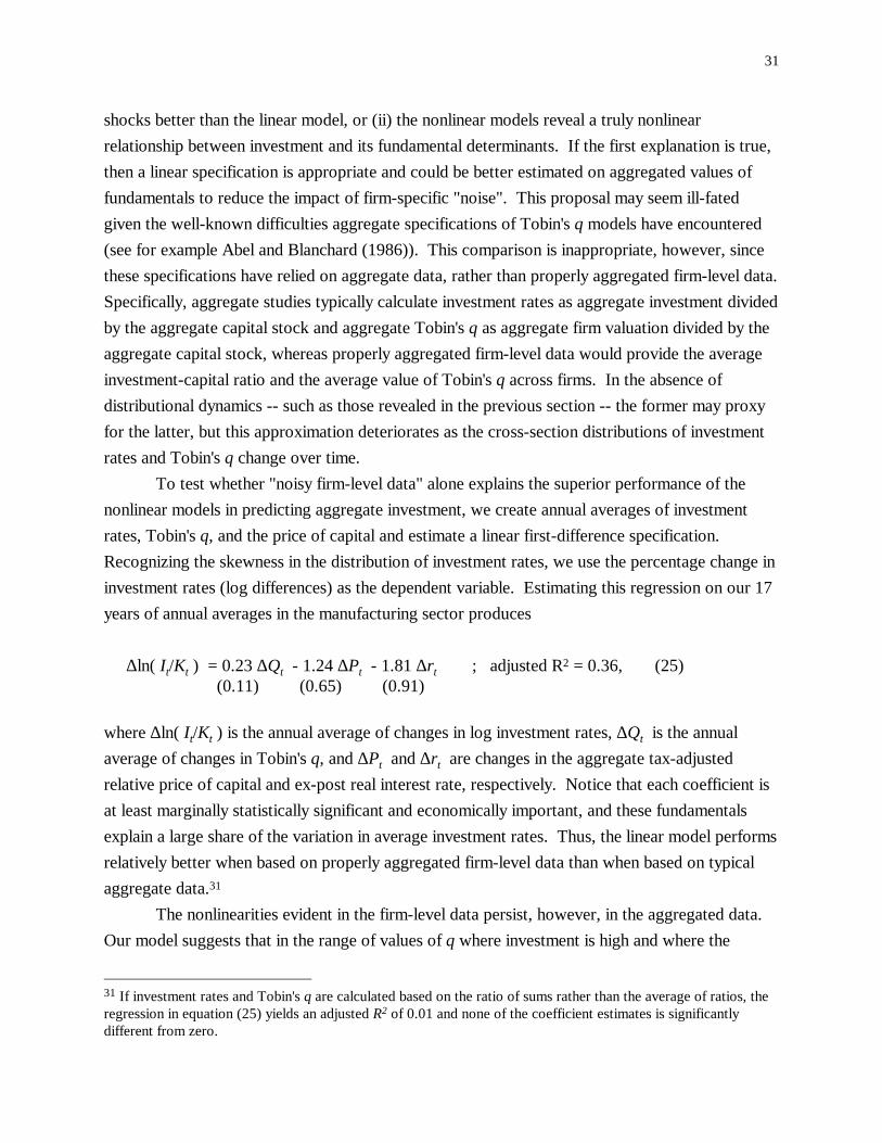
shocks better than the linear model, or (ii) the nonlinear models reveal a truly nonlinear relationship between investment and its fundamental determinants. If the first explanation is true, then a linear specification is appropriate and could be better estimated on aggregated values of fundamentals to reduce the impact of firm-specific "noise". This proposal may seem ill-fated given the well-known difficulties aggregate specifications of Tobin's q models have encountered (see for example Abel and Blanchard (1986)). This comparison is inappropriate, however, since these specifications have relied on aggregate data, rather than properly aggregated firm-level data. Specifically, aggregate studies typically calculate investment rates as aggregate investment divided by the aggregate capital stock and aggregate Tobin's q as aggregate firm valuation divided by the aggregate capital stock, whereas properly aggregated firm-level data would provide the average investment-capital ratio and the average value of Tobin's q across firms. In the absence of distributional dynamics -- such as those revealed in the previous section -- the former may proxy for the latter, but this approximation deteriorates as the cross-section distributions of investment rates and Tobin's q change over time.

To test whether "noisy firm-level data" alone explains the superior performance of the nonlinear models in predicting aggregate investment, we create annual averages of investment rates, Tobin's q, and the price of capital and estimate a linear first-difference specification. Recognizing the skewness in the distribution of investment rates, we use the percentage change in investment rates (log differences) as the dependent variable. Estimating this regression on our 17 years of annual averages in the manufacturing sector produces

∆ln( It/Kt ) = 0.23 ∆Qt - 1.24 ∆Pt - 1.81 ∆rt ; adjusted R2 = 0.36, (25)

(0.11) (0.65) (0.91)

where ∆ln( It/Kt ) is the annual average of changes in log investment rates, ∆Qt is the annual average of changes in Tobin's q, and ∆Pt and ∆rt are changes in the aggregate tax-adjusted relative price of capital and ex-post real interest rate, respectively. Notice that each coefficient is at least marginally statistically significant and economically important, and these fundamentals explain a large share of the variation in average investment rates. Thus, the linear model performs relatively better when based on properly aggregated firm-level data than when based on typical aggregate data.31

The nonlinearities evident in the firm-level data persist, however, in the aggregated data. Our model suggests that in the range of values of q where investment is high and where the

31 If investment rates and Tobin's q are calculated based on the ratio of sums rather than the average of ratios, the regression in equation (25) yields an adjusted R2 of 0.01 and none of the coefficient estimates is significantly different from zero.

32

dynamics in the distribution of q occur, the relationship between investment rates and q is concave. From Jensen's inequality, if this nonlinearity is present, greater cross-section variation in q should ceteris paribus depress investment. We test this implication by adding the annual cross-section standard deviation of q, std(qt), to the regression in equation (25), producing

∆ln( It/Kt ) = 0.34 ∆Qt - 1.46 ∆Pt - 1.62 ∆rt - 0.71 std(qt) ; adjusted R2 = 0.57. (26)

(0.10) (0.54) (0.76) (0.27) Notice that the inclusion of the cross-section standard deviation increases the magnitude and significance of the Tobin's q and capital price effects and increases the R2 by 21 percentage points to 0.57. The standard deviation itself has a significant negative effect on growth in investment rates; the effect is also economically significant (the mean of std(qt) is 1.02 and its standard deviation over time is 0.09). Thus, while using properly aggregated fundamentals and investment rates improves the performance of the linear model, accounting for distributional considerations substantially enhances the fit of the model -- and in the direction predicted by our nonlinear investment model. Since the results of the firm-level estimation emphasize changes in the upper tail of the distribution of q, we also examine the effect of skewness in q on aggregate investment growth rates. In equation (27) we replace the cross-section standard deviation of q by its skewness: ∆ln( It/Kt ) = 0.33 ∆Qt - 2.38 ∆Pt - 1.82 ∆rt - 0.28 skew(qt) ; adjusted R2 = 0.68. (27)

(0.08) (0.56) (0.65) (0.07) Interestingly, our coefficient estimates become more precise (and the capital price effect larger) and the adjusted R2 increases even further -- to 0.68 -- when skewness is used to measure distributional changes; here the adjusted R2 is almost doubled compared to the regression in (25) ignoring distributional effects. When the cross-section standard deviation and skewness are both included in the regression, the adjusted R2 falls (compared to that in (27) above) and the coefficient on the standard deviation becomes only -0.16 and insignificantly different from zero. These results are consistent with our interpretation of the firm-level data -- distributional dynamics occurring in the upper tail of q have an important impact on aggregate rates of investment. In particular, controlling for the mean, more dispersion of q in the upper tail depresses aggregate investment. When the standard deviation is included alone, it captures some of this effect, but skewness is a more focused measure of the dynamics within high values of q.32

32 The results reported in equations (25) through (27) are for the manufacturing sector, but the same pattern of results is obtained for non-manufacturing.

33

6. Conclusions

The literature on the q theory of investment has emphasized that the expected returns to investment are summarized by marginal q, which under certain conditions can be observed using average, or Tobin's, q. For a given investment cost function, q summarizes the incentive of the firm to change its capital stock. More recent, largely theoretical, work has focused on the possibility of irreversibility or fixed costs associated with investment and their effects on investment dynamics. This literature emphasizes the cost component of the optimality condition relating the costs and expected returns to additional capital. In this paper, we utilize essential elements of both strategies: we use Tobin's q to measure the expected returns to investment, and we allow for a general "augmented adjustment cost" function -- including fixed, linear, and convex costs of changing the capital stock. This specification nests the standard linear model, which we estimate as a benchmark, and underlies the two nonlinear investment equations estimated in sections 4.2 and 4.3.

The first nonlinear investment equation recognizes that convex adjustment costs need not be quadratic, so the relationship between investment and its fundamental determinants (q and the price of capital) need not be linear. Our estimates imply that this relationship is in fact concave, so the response of investment to fundamentals is always positive, but monotonically declining. Our second nonlinear investment specification explicitly accounts for capital heterogeneity and fixed costs of investment. Because of the fixed cost, firms do not choose to invest in every type of capital in every period, so the investment decision has both an extensive (which types of capital to buy) and an intensive (how much to invest in each type) margin. When fundamentals are low (that is, returns to capital are low and/or the prices of capital are high), firms choose to invest little and in few types of capital. As fundamentals improve, however, firms invest more in an increasing number of types -- producing a strong response of investment to fundamentals. Eventually, however, the extensive margin is exhausted, so when fundamentals are extremely strong, the response of investment reflects only the intensive margin.

This weakening of the response of investment to fundamentals when fundamentals are strong plays an important role in the predictive power of both nonlinear models. In particular, it implies that the distributions of q and prices affect aggregate investment, while these distributions are irrelevant to the linear model. In section 5, we show that the distribution of q, particularly its upper tail, changes cyclically; the nonlinear models use this information and accurately predict cyclical movements in aggregate investment, while the linear model, ignoring this information, systematically fails to predict these large changes in the investment-capital ratio.

We also consider disinvestment by firms, and find significant evidence of fixed costs. While disinvestment is not uncommon in our data -- 80 percent of the firms in our sample

34

disinvest at some point -- it is zero for about half of the observations. Our empirical analysis shows that disinvestment is associated with low values of q, which is far more successful at predicting the event of disinvestment than the amount. This is consistent with the presence of fixed costs of disinvestment, since returns must be sufficiently low to justify paying a fixed cost, but the quantity of disinvestment is then indeterminate.

These results suggest an important role for nonlinearities, potentially arising from fixed costs of investment, in understanding the relationship between investment and its determinants. The nonlinearities in our data are both statistically and economically significant; the data overwhelmingly reject excluding the nonlinear effects from the estimation procedure, and the nonlinear models systematically outperform the linear model in tracking annual averages of the aggregate investment-capital ratio. Using this criterion, it is difficult to distinguish between the predictions of our two nonlinear models, although these models differ markedly in their behavior at low values of the fundamentals. Data and experiments that highlight this range of data may be more successful in this regard.

35

References Abel, Andrew B., "Empirical Investment Equations: An Integrative Framework", Brunner, Karl and Allan Meltzer, editors, On the State of Macroeconomics, volume 12 of the Carnegie-Rochester Conference Series on Public Policy, 1980, pp. 39-91. Abel, Andrew B. and Olivier J. Blanchard, "The Present Value of Profits and Cyclical Movements in Investment," Econometrica 1986, pp. 249-273. Abel, Andrew B. and Janice C. Eberly, "A Unified Model of Investment Under Uncertainty," American Economic Review, 84, December 1994, pp. 1369-1384. Abel, Andrew B. and Janice C. Eberly, "Optimal Investment with Costly Reversibility," N.B.E.R. Working Paper #5091, April 1995. Barnett, Steven and Plutarchos Sakellaris, "Non-linear Response of Firm Investment to Q: Testing a Model of Convex and Non-convex Adjustment Costs," Mimeo, University of Maryland, August 1995. Bertola, Guiseppe and Ricardo Caballero, "Irreversibility and Aggregate Investment," Review of Economic Studies, 61, 1994, pp. 223-246. Caballero, Ricardo and Eduardo M.R.A. Engel, "Explaining Investment Dynamics in U.S. Manufacturing: A Generalized (S,s) Approach," N.B.E.R. Working Paper #4887, October 1994. Caballero, Ricardo, Eduardo M.R.A. Engel, and John Haltiwanger, "Plant-Level Adjustment and Aggregate Investment Dynamics," forthcoming, Brookings Papers on Economic Activity, 1995:2. Chirinko, Robert S., "Business Fixed Investment Spending: A Critical Survey of Modeling Strategies, Empirical Results, and Policy Implications," Journal of Economic Literature, 31(4), 1993, pp. 1875-1911. Ciccolo, John H., Jr. "Four Essays on Monetary Policy", Unpublished Ph.d. Disseration, Yale University, May 1975. Dixit, Avinash and Robert S. Pindyck, Investment Under Uncertainty, Princeton, NJ: Princeton University Press, 1994. Doms, Mark and Timothy Dunne, "Capital Adjustment Patterns in Manufacturing Plants," Working Paper, U.S. Census Bureau, October 1994. Hayashi, Fumio, "Tobin's Marginal and Average q: A Neoclassical Interpretation," Econometrica, 50(1), January 1982, pp. 213-224. Jorgenson, Dale and Ralph Landau, Tax Reform and the Cost of Capital: an International Comparison, Washington, DC: Brookings Institution, 1993.

36

King, Mervyn and Don Fullerton, The Taxation of Income from Capital: a Comparative Study of the United States, the United Kingdom, Sweden, and West Germany; University of Chicago Press, Chicago, 1984. Mussa, Michael, "External and Internal Adjustment Costs and the Theory of Aggregate and Firm Investment," Economica, 44, May 1977, pp. 163-178. Pindyck, Robert S., "Irreversible Investment, Capacity Choice, and the Value of the Firm," American Economic Review, 78(5), December 1988, pp. 969-985. Salinger, Michael A. and Lawrence Summers, "Tax Reform and Corporate Investment: A Microeconomic Simulation Study," in Martin S. Feldstein, editor, Behavioral Simulation Methods in Tax Policy Analysis, University of Chicago Press, 1983, pp. 247-287. Summers, Lawrence, "Taxation and Corporate Investment: A q-Theory Approach," Brookings Papers on Economic Activity, 1981, pp. 67-127. Tobin, James, "A General Equilibrium Approach to Monetary Theory," Journal of Money, Credit, and Banking, 1, February 1969, pp. 15-29. von Furstenberg, George M., "Corporate Investment: Does Market Valuation Matter in the Aggregate?" Brookings Papers on Economic Activity, 1977, pp. 347-397.

37

A. Data Appendix

A.1 Sample Selection Our data is an unbalanced panel of firms drawn from the Compustat full-coverage data base for the years 1974 through 1993. These data include the publicly traded firms in the Compustat Industrial Data Base, as well as firms traded over-the-counter (OTC). The full data set includes 107,540 firm-year observations. We eliminate all observations for which the data footnotes indicate evidence of a merger, acquisition, or discontinued operation. This reduces the sample size to 100,649 observations. We also require that each observation have no missing data for capital expenditure, the beginning-of-period capital stock, operating profits, and Tobin's q (for capital sales, both reported zeros and missing data are taken to be zero values). This significantly reduces the available sample to 24,746 firm-year observations. We then verify the capital accumulation identity relating the end-of-period capital stock to the beginning-of-period capital stock; observations for which this identity does not hold (to within one percent of the beginning-of-period capital stock) are eliminated from the sample. This requirement eliminates six percent of the remaining sample (many due to missing data on the components of identity), leaving 23,320 observations. We then require that investment and disinvestment take on "sensible" values. Both capital expenditures and capital sales are required to be non-negative, and capital sales may not exceed the reported size of the capital stock. Operating losses may not exceed the value of the firm's capital stock, and operating profits may not exceed 2.5 times the value of the firm's capital stock. These requirements reduce the sample size to 20,225. In our estimation procedures, we also restrict Tobin's q to be positive, but less than 5. While the lower bound is theoretically justified, the upper bound is arbitrarily chosen in an attempt to limit the impact of measurement error. We extended the upper bound to 15 with negligible effects on our results; the difference added only 44 observations to the manufacturing sample and 52 to the non-manufacturing sample. First-differencing the estimation equation reduces the final sample used in statistical analysis to 5803 observations in manufacturing and 6272 observations in non-manufacturing, as indicated in the text tables.

38

A.2 Data Calculation This part of the appendix describes the calculation of variables used in the econometric estimation. Underlying annual data items from the Compustat data base are first listed, followed by the calculations underlying the constructed variables. Sources for non-Compustat items are given in parentheses.

Data used in Section 4: I+, investment: capital expenditures I-, disnvestment: capital sales π, operating profits: operating income after depreciation inventories: total inventories (end of period) debt: long-term debt (end of period) PPE, book value of capital: property, plant, and equipment (beginning of period) Pk, price of capital: implicit price deflator for nonresidential investment, Economic Report of the

President, 1994, Table B-3, p. 272. PPI, two-digit producer price index: Economic Report of the President, 1994, table B-66, p. 345. r, real interest rate: the difference between the annual return on six-month commercial paper

(Economic Report of the President, 1995, table B-72) and year-over-year inflation in the producer price index (Economic Report of the President, 1995, table B-67).

u, investment tax credit: obtained by year for 51 asset classes from Dale Jorgenson. These data were aggregated to the two-digit industry level using the BEA historical cost capital flow matrix (asset by industry by year). Specifically, the weight of asset type n in industry j (in year t) was calculated as w I In j t n j t n j t

n, , , , , ,≡ ∑ . The investment tax credit applied to industry

j in year t, uj,t, was then contructed as the weighted sum: u w uj t j n t j n tn

, , , , ,= ∑ .

z, value of depreciation allowances: obtained by year for 51 asset classes from Dale Jorgenson. These data were aggregated to the two-digit industry level using the BEA historical cost capital flow matrix (asset by industry by year). Specifically, the weight of asset type n in industry j (in year t) was calculated as w I In j t n j t n j t

n, , , , , ,≡ ∑ . The value of depreciation

allowances in industry j in year t, zj,t, was then contructed as the weighted sum: z w zj t j n t j n t

n, , , , ,= ∑ .

τ, corporate tax rate: obtained from King and Fullerton, table 6.4, and Fullerton and Karayannis (in Jorgenson and Landau), p. 343.

market value of equity: closing stock price times number of common shares outstanding (end of period) plus redemption value of preferred stock (end of period).

L, useful life of capital goods: by two-digit industry, the useful life of capital goods is calculated

as LN

PPE DEPR IDEPRj

j

i t i t i t

i ti j≡

+ +− −+

∈∑1 1 1, , ,

,

, where Nj is the number of firms, i, in industry j.

Using the double-declining balance method, the implied depreciation rate for industry j, δj, is 2/Lj.

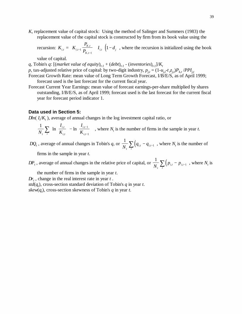
39

K, replacement value of capital stock: Using the method of Salinger and Summers (1983) the replacement value of the capital stock is constructed by firm from its book value using the

recursion: ( )K KP

PIi t i t

K t

K ti t j, ,

,

,,= +

−−

−1

1

1 δ , where the recursion is initialized using the book

value of capital. q, Tobin's q: [(market value of equity)t-1 + (debt)t-1 - (inventories)t-1]/Kt p, tax-adjusted relative price of capital: by two-digit industry, pj,t = (1-uj,t-τtzj,t)Pk,t /PPIj,t Forecast Growth Rate: mean value of Long Term Growth Forecast, I/B/E/S, as of April 1999;

forecast used is the last forecast for the current fiscal year. Forecast Current Year Earnings: mean value of forecast earnings-per-share multiplied by shares

outstanding, I/B/E/S, as of April 1999; forecast used is the last forecast for the current fiscal year for forecast period indicator 1.

Data used in Section 5: ∆ln( It/Kt ), average of annual changes in the log investment capital ratio, or

1 1

1NIK

IKt

i t

i t

i t

i tiln ln,

,

,

,

+−

+

−

−

∑ , where Nt is the number of firms in the sample in year t.

∆Qt , average of annual changes in Tobin's q, or ( )11N

q qt

i t i ti

, ,− −∑ , where Nt is the number of

firms in the sample in year t.

∆Pt , average of annual changes in the relative price of capital, or ( )11N

p pt

i t i ti

, ,− −∑ , where Nt is

the number of firms in the sample in year t. ∆rt , change in the real interest rate in year t . std(qt), cross-section standard deviation of Tobin's q in year t. skew(qt), cross-section skewness of Tobin's q in year t.

40

B. Calculation of Augmented Adjustment Costs In the model with heterogeneous capital in section 4.3, the linear component of investment costs may differ across types of capital. In calculating the implied costs of adjustment, we assumed that all of this variation was due to variation in the acquisition price of capital across types, and none of it due to the linear adjustment cost. In this appendix, we allow a share θ of the variation in the linear component to be due to adjustment costs. Thus, the calculations in the text implicitly imposed θ = 0. In the case with θ > 0, we rewrite the expression for augmented adjustment costs (as a share of the capital stock) in equation (13) according to

costs/K = ( )a vIK

v IK

dF qnn n

n

q

+ − +

∫ 1

22

20 2

θω ( ), . (B.1)

Substituting in the expression for optimal investment in capital of type n from equation (7) and simplifying, we obtain

costs/K =

aF qvv

q b v dF q

vq b v dF q

vq b v dF q

n n

q

n n n

q

n n

q

( ) ( ) ( )

( ) ( ) ( ) ( )

,

, ,

+ − − +

− − − + + − − +

∫

∫ ∫

1

21 2

0

21 2

0 21

22

0

12

ω

θ ω ω ω. (B.2)

This can be simplified by calculating the mean of a truncated normal distribution, and the last two terms can be simplified by calculating the expectation of the square of a variable with a truncated normal distribution. We can thus write total augmented adjustment costs (as a share of the capital stock) as

{ }

[ ]

1

22 1 2

21 1

12 1

2 2 2 21

2

21

vv q b v q b v G q b v

vq b g q b v

( ) [( ) ] ( )

( ) ( ).

− − + − − + + − − − −

− − + + − − −

µ σ θσ µ

σ θµ µ (B.3)

Note that the share, θ, of variability due to adjustment costs unambiguously decreases total adjustment costs. Thus, as noted in the text, the calculations made assuming θ = 0 are an upper bound on adjustment costs.

41