investigation of two diffusion problems using exact...
TRANSCRIPT

Investigation of two diffusion problems using exact
numerical methods:
I) Polymers in gels
II) Anomalous diffusion of particles in gels
by
Justin Boileau
A thesis submitted to
The School of Graduate Studies and Research
In partial fulfillment of the requirements
For the degree of Master of Physics
University of Ottawa
Ottawa, Ontario
May 11, 2004

ii
Summary
The concepts of diffusion and random walk have helped increase our understanding
of the movement of molecules in biological, physical and chemical systems. The scope
of applicability of the theory of diffusion is truly limitless. The theoretical study of
diffusion was initially focussed on the movements of small particles in quenched media.
Although narrow, this field has increased our knowledge concerning the diffusion of
proteins along bio-membranes, the gel electrophoresis of particles for the purpose of
separation, and the development of micro-fabricated devices used to separate molecules.
In the first part of this thesis, we generalize an existing model used to find the exact
diffusion coefficient of small particles among immobile obstacles. The model is
expanded to include small oligomers and allows us to study the non-trivial effects of
molecular architecture on the diffusion of molecules both in solution and in the presence
of immobile obstacles.
The second part of this thesis deals with the short time anomalous diffusion of
particles in disordered media. Historically, the steady state solution of molecular
diffusion was studied and little to no effort was ever made towards an understanding of
how molecules reach steady-state dynamics. An exact enumeration model is proposed to
study the exact short-time dynamics of a particle in 3 dimensional space.

iii
Sommaire L’étude des processus de dérive et des marches aléatoires a amélioré notre
compréhension de la dynamique moléculaire des systèmes biologiques, physiques et
chimiques. Les champs d’applications de la théorie de diffusion sont très vastes.
Initialement, cette théorie visait à expliquer le mouvement de petites particules évoluant
dans des milieux denses. Aujourd’hui, elle nout permet de mieux comprendre plusieurs
phénomène importants, comme par exemple la diffusion des protéines le long des
membranes et l’électrophorèse des particules chargées. Elle facilite également le
dévelopement d’équipement de séparation de molécules à échelle microscopique.
Dans la première partie de cette thèse, nous généralisons un modèle de diffusion qui
nous permet de trouver des valeurs exactes pour la mobilité et le coefficient de diffusion
de particules simples se déplaçant sur un réseau. Nous modifions le modèle existant qui
ne permet que de calculer la mobilité et le coefficient de diffusion de petites molécules.
Cette généralisation nous permet d’étudier certaines conséquences non triviales de
l’architecture moléculaire sur la diffusion des molécles en solution et en présence
d’obstacles.
Dans la deuxième partie de la thèse, nous présentons un nouveau modèle pour l’étude
de la diffusion de particules pour de courts intervalles de temps. Traditionellement,
l’étude de la diffusion visait le mouvement des particles en état stationnaire et très peu
d’importance était accordée aux phénomènes transitoires. Nous proposons un modèle
d’énumération exacte pour l’étude de la diffusion à temps court des particules en trois
dimensions.

iv
Statement of Originality
The work presented in this thesis is, to the best of my knowledge, new and original.
It is my own work except for section 2.3 where I recapitulate an existing model published
by the group of G.W. Slater over the last 8 years. All theoretical advances presented in
this thesis derive from my own work with the helpful guidance of my supervisor. All
analytical and numerical results shown herein have been realized through my own Maple
IV and Fortran 77 codes.
Additionally, most results contained in chapters 2-6 have been published in the
following article:
• J. Boileau and G.W. Slater, “An exactly solvable Ogston model of gel
electrophoresis VI: Towards a theory for macromolecules”,
Electrophoresis, volume 22, pp. 673-683 (2001).
Furthermore, I had the opportunity to present my results at the following meetings:
• J. Boileau and G.W. Slater, “A lattice model of gel electrophoresis: A
theory towards macromolecules”, Poster presentation at the Annual
meeting of the Canadian Association of Physicists (CAP), June 2000,
Toronto.
• J. Boileau and G.W. Slater, “A lattice model of gel electrophoresis”, Oral
presentation at the semi-annual graduate student seminars of the Ottawa-
Carleton Institute for Physics (OCIP), May 2000, Ottawa.
Finally, I also had the opportunity to participate in a review article written jointly by
the group of G. W. Slater:
• Gary W. Slater, Claude Desruisseaux, Sylvain J. Hubert, Jean-François
Mercier, Josée Labrie, Justin Boileau, Frédéric Tessier, Marc P. Pépin,
Theory of DNA electrophoresis: A look at some current challenges,
Electrophoresis, volume 21, pp. 3873-3887 (2000).

v
Acknowledgements
I would first like to thank my supervisor Dr. Gary W. Slater. His constant devotion
to the sciences, his continuous support and generous commitment of time have been key
factors towards the completion of my Masters degree. You have greatly enriched my
commitment to learning and been an inspiration that I can carry forward for the rest of
my life.
I would also like to thank Jean-François Mercier whose previous work and helpful
discussions has been a tremendous asset to the completion of this project. Thank you
Jean-François.
To Frederic Tessier I also give my heartfelt thanks for his help in both theoretical and
computational matters. Your experience and guidance have greatly enhanced the quality
of this work.
To the Department of Physics, both the support and research staff for their kindness
and devotion towards a productive research environment.
Lastly, but certainly not least, I would like to extend my gratitude to my wife, Crystal
Boileau, who has supported and encouraged my throughout. Your persistence, support
and faith in me have allowed me to bring this project to fruition. Thank you for
believing in me, I could not have done it without you.

vi
Table of Contents
Summary ii
Sommaire iii
Statement of Originality iv
Acknowledgements v
Table of Content vi
List of Figures viii
List of Tables xii
PART I:
1. Introduction ……………………………………………………………………………..1
1.1 Introduction to Polymer Physics…………………………………………...….….2
1.2. Molecular Dynamics Simulations……………………………..………..……..…6
1.3. Electrophoresis………………………………………….……………….….........7
1.4. The Ogston or OMRC Model…………………………….………………………8
1.5 Presentation of the Thesis………………………….…………………………….9
2. Numerically Exact Diffusion Coefficients and Electrophoretic Mobilities………..….11
2.1. Introduction…………………………………………….……………….….........11
2.2. Free Diffusion and Drift on a Lattice……………………………………..….…12
2.3. Lattice Model of Gel Electrophoresis……………..….…………………….…..16
2.4. The Bond Fluctuation Model & Polymers………………………….………..…19
2.5 The Generalized Model……………………………………………………….....21
2.6 Enumerating the Phase Space……………………………………………..…….23
3. Polymers in One Dimension………………………………………………….……...26
4. Polymers in Two Dimensions…………………………………………………….….32
4.1 Introduction……………….…..…………………………………………….…...32

vii
4.2. Example 2: Flexible Polymer in a Lattice of Dense Periodic Obstacles……..…33
4.3. Theory…………………………………………………………….………..……35
4.4. Free Macromolecules: Results…………………………………..……………....36
4.4.1 Flexible linear chains……………..……………………….…………….....36
4.4.2 Stiff Chains…………………………..………………….….……………...39
4.4.3 Ring Chains……………………………..………………….……………...40
4.4.4. Star chains…………………………………..……………….…................42
4.5. Conclusion…………………………………….………….…………………44
5. Molecules with the Presence of Obstacles: Results………………………….………45
5.1. Theory…………………………….……………………………………..….…..46
5.2. Periodic Gels…………………………………………………………..………..47
5.3. Anisotropic periodic Gels………………………………………………..……..54
5.4. Tubes…………………………………………………………...................…….58
6. Discussion………………………………………………………………......…...……62
PART II :
7. Anomolous Diffusion…………………………………………………...……..………65
7.1 Introduction……………………………………………………….………..…….65
7.2. Theory…………………………………………………………….……..………66
7.3. The model……………...………………………………………….……..……...70
8. Anomalous Diffusion: Results………………………………………………………...73
8.1 Validation of the Model (ε=0)……………………………………….……...…...73
8.2 Results in the Presence of a Field………………..………………….........……...81
8.2.1 Periodic Fibres………………………………………………………..…....82
8.2.2 A System with Periodic Traps………...………………………...……..…..90
8.3 Discussion………………..………………………………………………….…..99
PART III :
9. Conclusion……………………………………………………………………….……99
References…………………………………………………………...……………..….102

viii
List of Figures 2.1 Illustrative example of a lattice system in 2 dimensions with the
presence of obstacles…………………………………………………...
13
2.2 Schematic representation of the rules governing the bond fluctuation
model as it applies to various types of molecules……………………...
21
2.3 Schematic representation of a linear polymer in a lattice to show how
the enumeration of system states is performed ……………………...
25
3.1 Schematic representation of all system states of a linear one-
dimensional polymer…………………………………………………...
27
3.2 Plot of µ(M), R(M) and µR(M) for a 1D linear chain………………….. 30
4.1 Schematic representation of sample two-dimensional systems that will
be studied……………………………………………………………….
33
4.2A Scaling exponents υ of the end-to-end distance 2h vs M1 ............... 38
4.2B scaling exponent α of the diffusion constant D vs M1 ……................. 39
4.3 log-log plot of the diffusion coefficient D vs. molecular weight M of
the star chain in solution ……………………………………………….
43
4.4 finite-size scaling parameter α(M) vs. molecular weight M……………… 44
5.1 The scaled mobility, µ*, vs the concentration, C, for various molecules
of various molecular sizes……………………………………………...
48
5.2 The square root of the retardation factor, k½ , vs the radius of gyration,
Rg of various molecules……………………………………………….
49
5.3A Ferguson plot ln(µ*) vs the concentration, C, for circular molecules in a
periodic gel…………………………………………………………...
51
5.3B Ferguson plot (ln(µ*) vs Concentration) for flexible linear chains in a
periodic gel……………………………………………………………...
51

ix
5.4A Log-Log plot of the diffusion constant, D, vs the molecular weight, M,
of a flexible linear polymer in a dense lattice of obstacles (P=4)……....
51
5.4B The scaling parameter υ of the end-to-end distance 2h vs M1 for
flexible linear polymers in a dense lattice of periodic obstacles (P=4)...
54
5.4C The scaling parameter, α, of the diffusion constant vs M1 for flexible
linear polymers in a dense lattice of periodic obstacles (P=4)…………
54
5.5 The scaled mobility, µ*, vs the horizontal spacing, Lx, for flexible
linear polymers in a periodic anisotropic lattice of obstacles
(Lx>Ly=4)……………………………………………………………….
55
5.6 Figure 5.6: A schematic depiction of how the orientation factor S is
found for linear polymers……………………………………………...
56
5.7 The orientation factor, S, vs the horizontal spacing, Lx, of a flexible
polymer (M=3) in a periodic anisotropic lattice (Lx>Ly=4)……………
56
5.8 The scaling parameter, α, of the diffusion constant vs M1 for a linear
flexible polymer in a narrow tube (Ly=3)………………………………
58
5.9 Log-Log plot of the diffusion constant, D, vs molecular weight, M, of a
flexible linear polymer confined in a narrow tube interspersed with
confining walls…………………………………………………………
59
5.10 Schematic representation of a polymer in a tube with obstacles that
serve as entropic traps…………………………………………………..
60
5.11 Diffusion scaling parameter α vs. M1 of a flexible polymer in a
narrow tube (Ly=3)……………………………………………………...
60
5.12 Log (µ*) vs Log (M) for the tunnel system…………………………….. 61
7.1 Results of Starchev et al.16 for the scaling of the diffusion constant of a
latex bean in an agarose gel…………………………………………….
69
7.2A)
B)
Results of Starchev et al.16 for the mean displacement of a latex bead in
an agarose gel………………………………………………………...
70
7.3 Schematic representation of the distribution of probabilities in 2-
dimensions………………………………………………………………
71
8.1 Diffusion constant vs. time of a particle in a lattice without obstacles… 74

x
8.2 Log-log plot of the mean square displacement of a particle vs. time in a
lattice without obstacles………………………………………………...
75
8.3 Anomalous diffusion exponent, dw,x vs. time of a particle in a lattice of
periodic obstacles and a schematic representation of lattice……………
76
8.4 Anomalous diffusion exponent, dw,x vs. time of a particle in a lattice of
infinite periodic fibres and a schematic representation of lattice……….
77
8.5A Anomalous diffusion coefficient, dw,x, vs. time in a lattice of infinite
periodic fibres for several periodicities…………………………………
78
8.5B tmax vs. periodicity in a lattice of periodic infinite fibres……………….. 78
8.6 Log-log plot of the mean square displacement vs. time of a particle in a
lattice of infinite periodic fibers (P=3)………………………………….
79
8.7A The anomalous diffusion coefficient, D(t) vs. time of a particle in a
lattice of infinite periodic fibers (P=4)………………………………….
80
8.7B Log-log plot of (D(t)-Do) vs. 1/t of a particle in a lattice of infinite
periodic fibers (P=4)……………………………………………………
80
8.8 (dw-2) vs. 1/t for a particle in a lattice of infinite periodic fibers for
several periodicities……………………………………………………..
81
8.9A Mean displacement of a particle vs. time of a particle in a lattice of
infinite periodic fibers (P=3) in the presence of an external field
(ε=0.38)………………………………………………………………….
82
8.9B Mean square displacement of a particle vs. time of a particle in a lattice
of infinite periodic fibres (P=3) in the presence of an external field
(ε=0.38)………………………………………………………………….
82
8.10 Log-log plot of ( )2xx ∆−∆ and ( )2yy ∆−∆ vs. time of a particle
in a lattice of infinite periodic fibres (P=3) in the presence of an
electric field (ε=0.38)…………………………………………………...
83
8.11 xwd ,2 vs. concentration, C of a particle in a lattice of infinite fibers for
2 values of the external field……………………………………………
85

xi
8.12 xwd ,2 vs. time of a particle in a lattice of periodic fibers (P=3) for
various values of the external field……………………………………..
86
8.13A xwd ,2 vs. time of a particle ina lattice of periodic fibers in the presence
of an external field (ε=0.38) for several periodicities…………………..
87
8.13B xwd ,2 vs. time of a particle ina lattice of periodic fibers in the presence
of an external field (ε=0.30) for several periodicities…………………..
87
8.14 Schematic representation of the periodic funnel shaped lattice………... 90
8.15A xwd ,2 vs. time of a particle in a lattice of periodic traps for various
values of the external field……………………………………………...
91
8.15B ywd ,2 vs. time of a particle in a lattice of periodic funnel-shaped traps
for various values of the external field………………………………….
91
8.16 yx , vs. time of a particle in a lattice of periodic funnel-shaped
traps in the presence of an external field (ε=0.2)……………………….
92
8.17 Log-log plot of 22 , yx vs. time of a particle in a lattice of periodic
funnel-shaped traps in the presence of an external field (ε=0.2)………..
92
8.18 (dw.x-2) vs. t1 of a particle in a lattice of periodic funnel-shaped traps
for several values of the external field………………………………….
93
8.19 Log-log plot of the second moment of displacement (x,y) vs. time of a
particle in a lattice of periodic funnel-shaped traps in the presence of
an external field (ε=0.3)…………………………………………………
94

xii
List of Tables
4.1 Results of a flexible polymer in solution……………………………… 37
4.2 Results of a stiff linear polymer in solution…………………………… 40
4.3 Results of a circular or ring polymer in solution………………………. 41
4.4 Ratio of the radii of gyration of linear and circular polymers in
solution………………………………………………………………….
41
4.5 Results of a star chain in solution……………………………………… 43
5.1 Coefficients of the polynomial expansion of the scaled mobility, µ*,
for various molecules in a lattice of periodic obstacles………………..
47
5.2 Results of a flexible linear polymer in a dense lattice of periodic
obstacles…………………………………...............................................
52
5.3 Results of a flexible chain in a narrow tube……………………………. 60
6.1 Fit values of Ωo and Z of eq (6.1)………………………………............ 64

PART I
Chapter 1
Introduction
The movement of particles and small molecules, including polymers, in viscous and
porous media, has been a topic of considerable interest for many years. The study of
diffusion has helped us to understand many phenomena in chemistry, biology and
physics, ranging from the movement of molecules along cell membranes to protein
folding. These models have also helped to understand the dynamics of molecules in the
presence of a driving field, which has led to the development of sieving devices (e.g.
capillary electrophoresis1,2, ratchet-like devices3 and even DNA prisms4) used to separate
DNA molecules in support of the Human Genome Project. It is realistically a field of
limitless application and deserves all the attention that can be spared to it.
To study these problems, models have been developed such as the Lattice Monte
Carlo (LMC) and the Ogston-Morris-Rodbard-Chrambach (OMRC) models5-7. The
OMRC model is a mean field theory designed to study the movement of charged particles
in a liquid in the presence of an electric field, often referred to as electrophoresis. The
LMC model exploits the Brownian or random motion of particles along the framework of
a lattice to study static and dynamic properties of molecules. This thesis is divided in two
mutually exclusive parts. The first section deals with a model developed by Slater et al.8-
13 designed to find numerically exact diffusion coefficients of particles both in a good
solvent and within a lattice of steric obstacles. In my work, the model was improved to

2
include small polymers in those same conditions. Our study of this new model deals with
the free diffusion of oligomers, reptation problems, and finally entropic trapping devices.
The second part develops a numerical model which studies the short-time anomalous
diffusion of particles in various media. The short time dynamics of particles is a sub-
field of statistical physics that has not received much attention and deserves to be studied
more extensively in order to understand how a molecule reaches a state of steady
movement in its environment.
1.1 Introduction to Polymer physics Polymers are fascinating molecules that are applied and fabricated for virtually all our
day-to-day activities. The diversity with which polymers are used these days is truly
staggering. This section will give the reader enough background information on polymer
physics to allow navigation through this thesis without a great deal of previous expertise
in the field. We will begin by defining polymers and briefly describe their relevant static
and dynamic properties.
What is a polymer? From the most general point of view, any plastics or rubbers are
considered polymers. Your glasses are likely made of polymers. The “ink” on this page
is a polymer. From a scientific point of view the actual definition of a polymer may well
depend on whom you ask. A mathematician will tell you that it is a molecule whose
form is depicted as a random walk. A chemist will say that a polymer is a series of
identical molecules that are covalently bonded to form long chains. A physicist may
compare polymers with a fluid containing fewer degrees of freedom. While these
descriptions are essentially valid, they each provide only a portion of the answer to our
question. By taking each perspective into consideration, we achieve a better
understanding of what a polymer is.
So what makes the study of polymers so attractive? Firstly, polymers can both be
fabricated or found in nature. DNA molecules, for example, are considered polymers.
Secondly, dilute solutions of polymers can be seen as liquids whose molecules are not
strongly correlated to their neighbours. This makes their study far easier than a normal
fluid. For example, since polymers are strongly bonded in long chains, the shape of
individual monomers becomes unimportant on long time scales. In simple fluids,

3
geometrical effect associated with the shape of the molecules strongly affects the
behaviour. With polymers, the knowledge of just a few properties such as stiffness and
size allow us to accurately discern many thermodynamic properties. This inherent
simplicity is exploited to develop applications for use in industry. Let’s discuss some of
the properties polymers possess that we can study.
The number of monomers (M) forming a polymer molecule ranges from just a few
monomers (we then talk about oligomers) to over one million monomers. Typically, the
topology of a polymer is linear but the definition has lately been loosened to include ring
and branched polymers to name but a few. The monomers need not be identical
molecular subunits. A DNA molecule is considered a polymer with 4 different types of
monomer units that coalesce into a very specific structure (double helix). Polymers
whose monomers are identical are termed homopolymers while a polymer that has at
least 2 different monomers is called a heteropolymer.
The shape of a polymer molecule is the first step in understanding its behaviour. The
typical conformation of a linear polymer is much like a random walk, each monomer
positioned randomly in sequence. Several models were developed to study the shape and
size of linear polymers such as the freely jointed chain14. These models mirror the
concept that a polymer is shaped using random walk statistics but fail to account for the
physical dimensions of the individual monomers. This is known as the excluded volume
effect. Simply put, a monomer cannot occupy the same physical space as another
monomer. Taking the excluded volume into account will cause the molecule or
conformation to be larger than predicted by random walk models. This is called the
‘swelling’ of the polymer chain.
There are two popular properties by which the spatial size of a polymer is
characterized. The first is the mean end-to-end distance 2h , where hr
is simply the
(vector) distance between the first and last monomer and the brackets depict an ensemble
average. Another method is the molecule’s mean radius of gyration 2gR , which is an
average of every monomers’ square distance from the polymers’ centre of mass (CM),
mathematically defined by14:

4
( )∑=
−=M
iCMig RR
MR
1
22 1 rr (1.1)
where iRr
and CMRr
are the position of the i-th monomer and the position of the polymer’s
centre of mass, respectively. The values of 2gR and 2h will be a function of the
number and size of monomers and the stiffness imposed by the chemical bonds between
them.
Another aspect that we will study in this paper is the diffusion of polymers. To
understand how a polymer diffuses it would be useful to describe the displacement of a
single particle. The diffusion equation in one-dimension provides an excellent starting
point:
( ) ( )txPx
DtxPt o ,, 2
2
∂∂
=∂∂ (1.2)
where P(x,t) denotes the probability of a particle being at position x at time t and Do is the
diffusion constant. Solving this linear differential equation we obtain the first two
moments of the distribution function P(x,t)15:
tDx
x
o2
02 =
= (1.3)
where 2x is termed the mean square displacement. In d≥1 dimensions, the solution is
easily extrapolated to:
( ) tdDtr o22 = (1.4)
Eq (1.4) can be reordered to provide an expression for the diffusion constant:
( )dt
trDo 2
2
= (1.5)
This last expression defines the diffusion constant whether we are describing the motion
of a single particle or the centre of mass (CM) motion of a larger molecule (including
polymers). However, because one often observes transient effect for short times, it is
common to replace this relationship by:
( )t
tr
dD
to
2
lim21
∞→
= (1.5')

5
It is logical that the mean square displacement of a polymer molecule will be quite
different than that of a single particle. While eq (1.5) provides a universal definition of
the diffusion constant, the value of ( )tr 2 will be a function of the molecule being
studied. The Rouse model14 was developed to describe the dynamics of a polymer
molecule in solution. It is a bead-spring model that replaces solvent interactions with a
friction force, ξ and simulates the movement of the monomers using a stochastic force
fsto. The model considers neither hydrodynamic interactions nor the excluded volume
effect. The resulting equation of motion is called the Langevin equation and it can be
solved using simple mathematics. The Rouse model predicts that the mean square
displacement ( )tr 2 of the molecule’s CM is:
( ) tM
Tkdtr B
ζ22 = (1.6)
where kB is Boltzmann’s constant, T is the temperature, ξ is the friction coefficient of one
monomer and M is the number of monomers. Substituting with eq (1.5) we have for the
free solution diffusion constant:
ζMTkD B
o = (1.7)
or,
1−∝ MDo (1.8)
This model does not correspond well to experimental results since hydrodynamic
interactions are not taken into consideration. Nevertheless, the Rouse model is still very
important and has served as the basis of numerous theoretical investigations of polymer
dynamics in solutions14. Since our model also disregards hydrodynamic interactions, we
will be using the Rouse predictions to test our model’s validity. It is also important to
note that the Rouse model was intended for very long chains where the end effects
imposed by the first and last monomers can be neglected.
Of course, polymer dynamics may deviate from Rouse predictions depending on the
environment. For example, in a polymer melt, linear polymers will typically diffuse
along their backbone. Because of the high density of polymers, transverse diffusion is
inhibited. This type of movement is dubbed reptation and the restriction imposed on the
6
polymers’ degree of freedom will of course decrease the diffusion coefficient of the
polymer. The diffusion coefficient of a polymer chain undergoing reptation14 scales to
the order of: D~1/M2. Another example of an environment affecting diffusion is a
polymer chain inside a gel. Polymers and particles alike may then exhibit anomalous
diffusion due to the disordered nature of the gel-like structure. In other words, molecular
displacement may scale as: βtr ∝2 , where β<1, which does not correspond to
normal diffusion. It is often believed that the “anomalous” diffusion of particles in gels is
due to the fractal nature of the gel although there are no firm indications that the gels are
indeed fractal16. A safer statement would be that the anomalous diffusion of molecules is
linked with the level of disorder in the gel. The disorder will cause the chain to be
trapped in certain areas and flow freely where there is more available free volume. These
are but 2 common examples of situations where the diffusion of molecules may not
correspond to Rouse dynamics. Since molecules invariably diffuse in non-homogeneous
solutions, these special cases are truly relevant.
It is quite astounding that with these simple concepts of polymers such as shape and
movement, described using only basic mathematics and physics, we can predict the
behaviour of polymers in very complex systems. These basic building blocks will allow
a better comprehension throughout this work. The next 2 sections describe the
computational work that was historically accomplished to determine the behaviour of
polymers in quenched disordered systems.
1.2 Molecular Dynamics Simulations Before getting too far ahead of ourselves, let’s examine how the study of the
movement of particles began. By following through some historical notions we can gain
a better appreciation of how our work becomes a stepping stone towards the modelling of
more realistic systems. Brownian motion is the apparent random movement of particles
associated with the bombardment of a molecule with neighbouring particles. Early in the
20th century, Einstein formalised the concept by using statistical arguments and
introducing the random walk problem. The diffusion of particles has since been
modeled and observed as random walks. With the advent of computers, algorithms were
developed to study molecules by simulating their collective random motion. Thus the

7
study of Molecular Dynamics began. Although useful in theory, Molecular Dynamics
simulations require a large commitment of time and processing power. The proper
simulation of molecules requires several interactions to be considered simultaneously and
it can become very time consuming for a molecule to cover enough of phase space to
properly discern thermodynamic properties. It may thus become important to simplify
the models in a manner which do not compromise the physical behaviour of the system.
Randomly moving molecules along a lattice is a popular alternative to Molecular
Dynamics simulation. The Lattice Monte Carlo (LMC) algorithm is such an example.
This model simulates the movement of particles by making random jumps along the
framework of a lattice. The fact that the molecule is constrained in its movement by a
lattice allows the molecule to easily cover its phase space without undermining physical
properties. In other words, we generally retain the proper dynamics and thermodynamic
properties while greatly reducing the number of molecular degrees of freedom. The only
problem with LMC methods is that the fluid, which would be treated explicitly in
Molecular Dynamics simulations, is now replaced by stochastic rules. Consequently, the
precision becomes dependent upon the duration of the simulation, and collective fluid
effects (e.g. hydrodynamics) do not exist. Moreover, we rarely achieve a precision of
greater than 0.1%, which somewhat limits its scope of applicability.
Analytical models have also been developed as alternatives to allow researchers to
quickly and efficiently predict the approximate behaviour of molecules in given systems.
For a long time, the OMRC model (see Section 1.4) was considered one of the leading
methods for predicting the mobility of small molecules during gel electrophoresis.
1.3. Electrophoresis Electrophoresis is the study of the movement of charged particles immersed in a
liquid and subjected to an electric field. Much of the human genome project relied on
electrophoresis for the separation of DNA fragments2. Many sub-fields have been
developed for the electrophoretic separation of molecules. One such field is gel
electrophoresis. Molecules are immersed in a gel to counter electro-osmotic flow and
convection in the fluid. This causes the motion of the molecules to rely solely on the
electric force and their natural diffusion. The gel is usually a solution of cross-linked
8
polymers, like agarose, and molecular species are separated according to their size since
larger molecules collide more frequently with the gel and take longer to elute. Another
subfield is capillary gel electrophoresis2 where molecules are injected in a gel-filled
capillary and then separated. This offers a cheaper and faster alternative for the
separation of molecular (or ionic) species. Although this thesis investigates the
electrophoretic mobility of analytes, our analysis will be limited to very weak applied
fields. In this limit, the mobility is directly proportional to the diffusion coefficient;
therefore, our results are equally valid for the study of standard (zero-field) diffusion
problems.
1.4 The Ogston or OMRC Model The OMRC model, commonly referred to as the Ogston model, was first developed
to explain the sieving effect of the gel on the electrophoretic mobility of small
analytes5,6,17,18. The model was used to predict the electrophoretic mobility of charged
particles in inhomogeneous media such as agarose gels. These cross-linked gels offer a
sieving effect because larger molecules tend to collide more frequently with the gel fibres
thus impeding their motion. The typical quantity sought in electrophoresis experiments
is the mobility µ, defined as the drift velocity acquired by a particle divided by the
magnitude of the applied external field. This model links the electrophoretic mobility of
a solute with the volume available to it:
( ) ( ) )(0
* CFCC ==µµµ (1.9)
where C is the concentration, µ*(C) is the scaled mobility, µ(C) is the mobility, µo is the
mobility of the particle in the absence of a gel (C=0), and F(C) is the fraction of the total
gel volume available to the particle. The fraction µ(C)/µo is called the scaled mobility
(µ*) which is a useful quantity to isolate the effect of obstacles for a given system.
The Ogston model became so widely accepted that much effort was devoted to
finding the fractional available volume F(C). Ogston showed that F(C) for a spherical
particle in an array of randomly oriented fibres is given by an exponential function whose
only parameters are the size of the solute and gel fibres respectively. Indeed, the model
(apparently) correlated rather well to experiments using small molecules in randomly

9
arranged gels of low concentrations (far from the percolation limit). The simplicity of the
model was so attractive that molecular architecture even disappeared from the models. It
wasn’t until recently10,11,19,20 that the Ogston model was challenged for its apparent
lacunae. The OMRC model 5-7,13,17,18,21, shown to be equivalent to a mean field theory,
fails to consider the finer details of molecular interactions and trajectories.
Unfortunately, this model was never successfully verified using experimental
measurements due to the difficulty in measuring the scaled mobility µ*(C) and the
available volume F(C) independently.
The first part of this thesis (chapters 1 through 6) will put the OMRC model to a
continued test (since it was initially tested using rigid isotropic analytes). Of particular
importance is the fact that the OMRC model is still used quite extensively to analyze the
mobility of short polymers. This may appear a little counter-intuitive because the OMRC
model was designed for spherical and rigid molecules whereas a polymer is defined by a
linear sequence of like molecules that are covalently bonded. The reason for the apparent
validity of the OMRC model as applied to linear polymer molecules is because the shape
of a polymer appears to follow a random walk and the final average shape of the polymer
is more or less spherical in situations where gel concentrations are very low. Therefore,
for the purpose of the OMRC model, the polymer is often modelled as a spherical
molecule whose size is given by its radius of gyration, Rg, which is essentially a
reasonably valid mean field statement.
The fact remains that the Ogston model is still a mean field approximation that
disregards molecular details and the measure of disorder in a gel when predicting the
electrophoretic mobility of the molecule. We shall later demonstrate how both of these
factors can play a crucial role in the diffusion of molecules.
1.5 Presentation of the Thesis As mentioned before, this thesis is divided in two separate parts. The first part
studies the electrophoretic mobility of small oligomers in a vanishing electric field and is
subdivided as follows: Chapter 2 introduces the original model and reveals how we
improved the model to include molecular degrees of freedom. Chapter 3 presents and
discusses our results for the mobility of linear polymers in 1 dimension (1D). Chapter 4

10
extends our analysis to the study of polymers in 2D without the presence of obstacles.
Chapter 5 discusses the mobility of analytes in the presence of obstacles and finally,
Chapter 6 contains a discussion of the results obtained thus far. In chapter 7 we introduce
the second part of the thesis. We present a model for the study of the short time
anomalous biased diffusion of a single particle. We use an enumerative method to
analyse the progression of the diffusion constant towards the steady state regime. We
start by introducing theoretical concepts followed by a short introduction to the model.
We then utilize simple systems to validate the model before progressing to more complex
systems whose diffusive behaviour has been difficult to ascertain.

11
Chapter 2
Numerically Exact Diffusion Coefficients and
Electrophoretic Mobilities
2.1. Introduction Over the last few years, a new mathematical model was put forward to compute the
exact diffusion coefficients of rigid isotropic particles in various media8-13. This model
neglected hydrodynamic interactions and intra-molecular degrees of freedom but was
nevertheless an invaluable tool for the study of diffusion in porous media and provided
insight into the future possibilities of this field. Although it was extremely useful for the
study of point particles, it was unable to deal with certain important problems. Amongst
these are the diffusion and electrophoresis of rod-like molecules (viruses, short dsDNA
fragments, etc.), the dynamics of molecules of identical weight but with differing
architecture, the migration of soft globules or vesicles and the effects of conformational
entropy during electrophoresis. In this thesis we present a generalized version of the
model which includes intra-molecular degrees of freedom. This will give us the
opportunity to increase the scope of our study and gain a better understanding of the basic
principles governing the dynamics of polymers.
The purpose of this chapter is to present the model that will be used to study the
properties of small molecules. Since we are presenting an improvement to an existing
model developed by the group of Gary W. Slater, it will be necessary to first present the
original model. In section 2.2 we will discuss in general terms the diffusion constant and
the mobility of a particle in the presence of a weak electric field. We will also describe
how these concepts are applied when using a lattice model. In section 2.3 we will discuss

12
the lattice description that will be used to describe the molecules. The original model will
be presented in section 2.4. This will establish a theoretical foothold that will be
necessary to understand the generalization of the model. Sections 2.5 and 2.6 present the
improved model. We will discuss the necessary changes to the original model necessary
to accomplish the generalization. This new model will allow us to include, for the first
time, intra-molecular degrees of freedom in the electrophoretic study of molecules and
will permit us to study many more problems that were not within its original scope.
2.2. Free Diffusion and Drift on a Lattice We first examine the movement of a particle in a free solution (no obstacles). The
free solution electrophoretic mobility µo of an analyte is defined by the ratio of its
electrophoretic velocity ν to the electric field E15:
Ev
o =µ (2.1)
Typically, the mobility is defined by µ=ν/F. Since we are dealing with the steady state
motion of the particle, the acceleration becomes zero and the mobility is defined by its
terminal averaged velocity, hence µ= ν/E.15 In the absence of a driving force, the spatial
fluctuations of a particle of size R result from its thermal motion and the friction
coefficient f(R) resulting from the fluid’s viscosity. We then have a general expression
for the free solution diffusion constant Do:22
( )RfTkD B
o = (2.2)
The mean drift velocity in the presence of a driving force is given by the ratio of the
applied external force Fext to the friction coefficient f(R):22
( )RfF
v ext= (2.3)
In the special case where the external force is an electric field we have:
)(Rf
QEv = (2.4)
where Q is the charge of the particle. Combining eqs (2.1), (2.2) and (2.4) we have:

13
oB
o QTk
D µ= (2.5)
otherwise known as the Nerst-Einstein relation. The latter links the mobility µo with the
diffusion constant Do. This relation is generally valid only for low field intensities.
The lattice model used to describe the motion of a single particle is depicted in Figure
2.1. The particle can be located on any of the 7 numbered lattice sites and its size
coincides with the dimensions of the lattice sites (a x a). The Brownian time step
associated with each move is given by:
o
B Da
2
2
=τ (2.6)
where Do is the diffusion constant in free solution given by eq 2.2.
To define the probabilities associated with the discretized movement of particles we
will be using an approach developed by Slater and Rousseau23. This approach, which is
reminiscent of the Glauber24 approach, is summarized as follows:
Given a system of one charged particle in one dimension, the probability of jumping
in the ± x-direction in the presence of an electric field is given by:
( )( )3121 εεεε
ε
Oee
ep x +±≅+
= −+
±
± (2.7)
where ε is the scaled dimensionless value of the electric field given by:
Tk
QEa
B
=ε (2.8)
where Q is the charge of the particle. This probability function allows us to increase the
probability of movement in the +x direction and decrease it proportionally in the –x-
direction such that the normalization condition: (p+x+p-x=1) is still satisfied. The time
1
7
6
5
4
3 2
Figure 2.1: Conceptual drawing of the lattice model. The obstacle on the lattice is depicted by the black square. The physical dimensions the individual lattice sites is a x a. The available lattice sites are numbered 1 to 7. We use periodic boundary conditions along both Cartesian axes.

14
step associated with these jumps is thus also changed by the presence of an external
electric field:25
( )Bτε
ετ tanh= (2.9)
or, we can use a dimensionless value of time, defined by:
( )εε
τττ tanh* ==
B
(2.10)
For ε<<1 we can expand eq (2.10):
( )42
*
31 εετ O+−≈ (2.11)
This expansion is of particular importance since it will allow us to simplify the problem.
Note that while the time step, τ*, is a function of the applied electric field, eq (2.11)
reveals that the time step is not perturbed to the first order of ε. This means that the
jumps will be evenly distributed in time regardless of the direction of movement as long
as the second order term of the scaled electric field remains negligeable. We can also
make use of a dimensionless expression for the velocity:
a
v Bτυ = (2.12)
Using eq (2.10) we can derive a dimensionless expression for the velocity of our particle
in terms of probabilities:
( )( )( ) ε
εεετ
ττ
τυ εε
εε
==×+−
=×−
= −+
−+−+
tanhtanh
aeeee
app BBxx (2.13)
Combining (2.13) and eq (2.8) we have a dimensionless expression for zero-field
mobility of a molecule:
.1lim0
==→ ε
υµε
o (2.14)
Using eq (1.9) and the Nerst-Einstein relation (eq 2.5) we can relate the scaled values of
the mobility and the diffusion constant of our particle:
** DDD
oo
===µµµ (2.15)
Note again that this is generally valid only in the ε→0 limit. Defining these scaled
quantities is a useful tool by which we can isolate the effect of obstacles on the mobility

15
and diffusion constants. It can also then be claimed that this model is appropriate for the
study of the zero field diffusion of particles in gels.
Finally, extending our analysis to 2 dimensions and in the limit of small ε we have:
( )32 4
11
11 εεε O
edp x +
±≈
+=± m
41
21
==± dp y (2.16)
where d=2 is the dimensionality.
By now, it has become quite clear that we plan on conducting a dimensionless
analysis of results. This approach allows us to apply our results to a plethora of polymer
systems without having to consider the finer details of a specific polymer system such as
stiffness and individual monomer composition. Consequently, a dimensionless analysis
is more conducive to our goals. Unfortunately, it is also useful to give experimentalists
an idea of how our results can be applied in practice. We will now offer an approximate
analysis of how our results would compare to experimental results by relating the length
and time scales associated with our lattice system.
By linking the contour length oc bML )1( −= of a polymer chain (where M is the
number of monomers and bo~2.89 from the BFM) with the persistence length
cp LhL 22= (where h2=(M-1)b2) we have: lp~5 lattice spacings would be a reasonable
value. Given that the persistence length of a double stranded DNA is 53nm with each
base pair measuring bp~0.38 nm, we have 1 lattice site=30bp~10nm. From here we can
compute the relaxation time through the molecules’ radius of gyration and diffusion
constant through the relations14:
τ
πη
4/
62
gRD
RTkD gB
=
= (2.17)
Isolating for τ we have: Bg kR 46 3πητ = ~10µsec (using typical values of the solution
viscosity and radius of gyration). Linking the relaxation time with the number of Monte
Carlo Steps (MCS)29 we can compute the time step for each MCS. We then arrive at an
approximate solution of τ~1/4 µsec.

16
2.3. Lattice Model of Gel Electrophoresis This section describes the original lattice model of Slater and co-workers. For a more
complete overview of the model along with detailed examples refer to [8-13,21]. Now
that we have defined the probabilities associated with the movement of a particle and the
appropriate dimensionless quantities, we can proceed to explain the details of the lattice
model. Referring once again to Figure 2.1 we see a lattice in two-dimensions containing
S=7 available sites which are numbered for clarity. In this lattice model, we will be using
periodic boundary conditions (PBC). Referring to the lattice system in Figure 2.1, a
particle moving from site number 7 in the +x direction would reappear at site 2.
Likewise, a particle at site 3 moving in the ±y direction would remain at site 3 due to the
obstacle depicted by the blackened square. Using PBC, we can simulate an infinite
volume in which the particle can evolve.
As mentioned, any such lattice will have S available sites in which the particle can be
legally placed (ie: a site which does not have an obstacle). To find the mobility of the
particle in our lattice system we will rewrite eq (2.14) and (2.15) to correspond more
appropriately to our lattice system:
εµ
µε o
nvD lim
0
**
→
== (2.18)
where n is the vector whose elements ni correspond to the probability of the particle
being located at site i=1..S in the steady-state. v is the vector whose elements υi
correspond with the particle's velocity while located at site i=1..S in the steady-state.
Note that we use Dirac notation in this work: bras and kets represent Row and Column
vectors ( n and n ), while uppercase and lower case letters depict matrices and scalars
respectively. The rationale behind eq (2.18) is that the presence of an external field will
create anisotropy in the system causing the probability of occupation of the particle to be
a function of its position (i) within the lattice. Equation 2.18 is simply the weighted
average over all sites.
Using eq (2.16) for the probabilities we can write linear equations of motion
corresponding to the probability of a particle being located on a lattice cell. Generally, we
have for nx,y(t+1):
17
( ) ( ) ( ) ( )tnptnptnptnptn yxyxyxyxyx 1,1,,1,1, )(1 +↓−↑+←−→ +++=+ (2.19)
As an example, for the lattice shown in Figure 2.1 we have for ( )11 +tn :
( ) ( ) ( ) ( )tnptnptnptn 6211 1 →↑→ ++=+ (2.20)
A similar equation can be written for the six other sites. We can rewrite the system of
equations to include all 7 equations as:
( ) ( )1+= tntnT (2.21)
where T is an SxS transition matrix whose elements denote the transition probabilities
from one system state to the next and ( ) ( ) ( ) ( ) tntntntn 721 ,...,,= is the probability
vector. Given that we are dealing with the steady state solution of the mobility we have:
( ) ( )1+= tntn (2.22)
meaning that we can re-write eq (2.20) as:
( ) ( )tntnT = (2.23)
and, by factoring we obtain,
( ) 0=− nIT (2.24)
where I is the Identity matrix and 0 is the null vector.
Before we can solve the system of equations shown in Eq (2.24) we must
acknowledge that eq (2.24) has only (S-1) independent equations. We must then impose
a normalization condition. Replacing the last row (by convention) of the matrix T with
∑ =i
in 1 (2.25)
accounts for the fact that the sum of all probabilities is always 1. Equation (2.24) then
becomes:
bnA = (2.26)
where b = 0, … , 1 and A is the matrix modified by including a normalization
condition to the transition matrix T.
Recall that to find the mobility of the particle we had to link the particle’s velocity
with the local probability (eq. 2.16). The velocity of the particle is defined quite simply.
We have for the components iυ of υ :

18
←←→→ −= LpLpiυ (2.27)
where the probabilities p→,← are defined by eq (2.16) and L→,← = 0 if the jump is
illegal and L→,←=1 is the jump is accepted.
Using eq (2.25) to find probability vector n and eq (2.27) to define the velocity vector
υ we have all that we need to find the particle’s mean mobility. The only remaining
issue is that the probability and mobility equations are a function of the, as yet undefined,
parameter ε. To circumvent having to define a specific numerical value to the scaled
electric field, ε, we use a useful algebraic simplification. Writing each mathematical
object A, n and v as the sum of field-independent and (first order) field-dependent
terms we have:
εεAAA I += (2.28)
εε nnn I += (2.29)
ευευυ += I (2.30)
Replacing eq (2.28) and (2.29) into eq (2.26) we have:
( ) IIIII bnAnAnAnA =+++ εεεε εε 2 (2.31)
To first order in ε we are reduced to 2 equations:
III bnA = (2.32)
II nAnA εε −= (2.33)
The first of the two equations shown above corresponds to the trivial case without the
presence of applied electric field and leads to the homogeneous solution Sni1= .
Equation (2.33) deals with the non-trivial effect of fixed obstacles being introduced into
the system in the presence of a driving force. The presence of obstacles removes the
translation symmetry of the system effectively skewing the probabilities. Since AI, Aε,
and nI are all quantities that can be readily found without calculation we only need to
solve for the vector εn . With this in mind we will go over an identical simplification
done in terms of the particle’s velocity.
Clearly, the velocity of the particle must be a function of the particle’s local
probability of presence. Using eq (2.30) we have:

19
( ) ( )( ) ( )2ευυευ
ευευυυ
εε
εε
Onnn
nnn
IIII
II
+++=
+⋅+== (2.34)
The first term on the right hand side (RHS) of eq (2.34) is zero since it corresponds to the
velocity in the absence of an applied electric field. Ignoring the term in ε2 we are left
with the term in ε1. Finally, using eq (2.18) for the mobility and eq (2.15) the scaled
mobility we have:
( ) ** D
nn
o
II =+
=µ
υυµ εε (2.35)
We see that the value of the low-field scaled mobility is no longer a function of the scaled
electric field! Therefore, using this simplification, we do not have to declare any value of
the scaled electric field to the first order. This simplification can only be used in the
presence of a small electric field where second order terms can be neglected. A stronger
field would force us to consider these second order terms and oblige us to reconsider
using a uniform time step. References [8-13] provide a detailed derivation of these
simplifications and provide useful examples.
So far in this chapter, we have introduced a model that can allow us to compute the
electrophoretic mobility and the diffusion coefficient of a particle in a vanishing electric
field. We have seen that, using a simple probabilistic approach, we can reduce this
seemingly complex problem to solving a system of equations where each unknown
corresponds to the probability of occupation of a lattice site. We also applied an
algebraic simplification that relieved us of the responsibility of having to declare an
arbitrary value of the applied electric field. In the following section I describe the rules
governing the behaviour of polymeric molecules on a lattice. In other words, I will
present that lattice description of my generalized model.
2.4 The Bond Fluctuation Model for Polymers In section 2.3 we described the original model as it pertains to a particle evolving on
the framework of a lattice. Our goal in this thesis is to generalize the model to include
small flexible polymers and molecules. The first step towards this end is to provide a
lattice description of the molecules studied. Several models for the simulation of
polymers already exist. We require a model that properly simulates both the static and

20
dynamic properties of polymers. Additionally, we want a lattice description that allows
for the simulation of both two and three-dimensional polymers. Finally, it is important
that the model be able to study molecules that are not strictly linear. One of the goals of
this project is to study ring and star polymers as well as linear polymers. It would be
fruitless to compare results if we were obligated to use a different lattice description with
different types of molecules. Despite our previous statement that any bond description
could be used with this model our needs have greatly limited the number of descriptors
which were deemed adequate for the purpose of this study.
The Bond Fluctuation Model (BFM)26 was chosen to describe macromolecular
dynamics in this thesis. This model was selected because it represents a self-avoiding
walk and the simulation algorithm is ergodic in two and three dimensions. The model
exhibits proper Rouse dynamics and the radius of gyration scales according to the Flory
exponent in LMC simulations thus exhibiting proper static properties. Moreover, the
variable bond length increases the ‘realism’ of the macromolecule being studied.
Although initially devised with linear polymers in mind the BFM can be used to study
other types of molecules such as ring and branched polymers. For completeness, the
model will be briefly described. Refer to [26] for a more detailed description and
analysis of this lattice model.
The BFM can be used in both 2 and 3 dimensional studies. The precept of the model
is that the bond length between 2 connected monomers is variable. In 2 dimensions, a
maximum bond length of less than l=161/2 was chosen between 2 connected monomers.
This restriction was necessary to avoid bond cutting. Furthermore, the minimum
distance between any two monomers is l=2. This fulfills our excluded volume
requirement since this restriction ensures that 2 monomers do not occupy sites adjacent to
one another. Figure 2.2 shows four two-dimensional systems based on the BFM. This
model's high coordination number in two dimensions (Z=36, meaning that a second
monomer can find itself bound to the first in 36 different positions) can be seen as a
disadvantage because it will greatly limit the size of molecule that we will be able to
study. Nevertheless, we chose this algorithm because of the realism it conveyed with
regards to polymer dynamics and static polymer descriptions.

21
A B
C D
E
The following section will introduce the generalized model.
2.5. The Generalized Model As mentioned, the model discussed in section 2.3 can allow us to compute the exact
diffusion coefficient of a particle evolving in an obstacle-laden environment. It has been
demonstrated that using this model offers many advantages over the more traditional
lattice Monte Carlo algorithms. In this section we will go over the fundamental changes
that were necessary to allow for the study of small flexible molecules. Once we have
developed the generalized model we will be able to study their static and dynamic
properties. Our first challenge to generalize this model is to consider the
conformational phase space of the molecule when enumerating the possible states of the
system. Using the assumption that the molecular conformations and the position of the
molecule are independent quantities will greatly simplify this task. In fact, given that the
system is ergodic, there is no reason to believe that our assumption is false. The model
introduced in section 2.3 enumerated the system states based on position alone. This
Figure 2.2: Four different two-dimensional systems based on the bond fluctuation model. Circles represent the monomers. Arrows show the possible moves of single monomer jumps, the blackened squares represent obstacles, and the shaded area in Figures 1A, 1B and 1C show the allowable positions of the next monomer in the chain following the monomer depicted by a filled circle. A) A free linear chain with M=4 monomers; B) The same chain in a lattice of periodic obstacles representing the densest gel. Obstacle plaquettes are placed periodically with lattice parameters Lx=Ly=4. We see that the obstacles follow the same excluded volume rules as depicted by the bond fluctuation model; C) A semi-rigid linear chain with M=4 monomers in a narrow tube. The angle θ between two consecutive bonds are restricted to |θ| ≤ π/4. D) A linked or circular chain is shown with M=5 monomers. E) A star polymer with all monomers linked to the centre and all branches have only 1 monomer.

22
model will need to include the molecular conformation as well as the position when
determining the states our molecule can have. Molecular states can then be viewed as
possessing two “properties”: The first is position and the second is conformation. The
total number of states, S′, will then be a function of both of these properties and is given
by:
∑=
=′S
kkFS
1 (2.36A)
where S is the number of available sites and Fk is the total number of conformations
allowable on site k. The quantity Fk is a function of the position of the molecule since
interactions with obstacles will limit the allowable number of conformations. Section 2.6
discusses the exact procedure used to enumerate the possible states of the system. They
would be named (k,Ci), where k is the position of monomer 1 and Ci is the conformation
of the molecule. We then clearly have:
∑= LFk (2.36B)
where the summation is over the total number of conformations and L=1 if the
conformation Ci is legal for position k and zero otherwise.
When we presented the original model we discussed how the probabilities associated
with a change of state is based on the Glauber approach. Specifically, eq (2.16) deals
with the probabilities of transition when only 1 particle is used. Clearly, eq (2.16) is no
longer applicable when we have more than one monomer to consider. To account for the
added monomers we must redefine the way the transition is made. Since we define all
monomers as being equally likely to make a move we define our probabilities to account
for the fact that our molecule consists of M monomers:
dM
P2
11,
ε±⋅=→← (2.37)
dMP
211
, ⋅=↓↑ (2.38)
The final step used to generalize the model is defining the velocity of the molecule.
The original model used the simple relation shown in eq (2.27) to find particle velocities.
Our first thoughts towards finding the molecular velocity were to use eq (2.27) and apply
it to each particle in the molecule. Taking the subsequent average is an effective way to

23
ensure the proper velocity is found. Another method to find the molecular velocity was
found which minimizes the computing time. We reasoned that taking a reference
monomer would yield the same result since the reference monomer is restricted to
following the centre of mass (CM) of the molecule. Our reasoning turned out to be
correct (results not shown) and we will be choosing the first monomer of any molecule
by convention when determining both the position and the mean velocity of the molecule.
2.6. Enumerating the Phase Space Having discussed how the probabilities and the velocity equations were modified in
the generalized model, we need only discuss how the enumeration of states is
accomplished. We also discussed how the system states are defined using 2 properties:
the position of the first monomer and the molecule’s conformation. This system state is
annotated: (k,Ci), where k=(x,y) is the position of the molecule on the lattice and Ci
represents the molecule’s conformation.
Obviously, the two properties of the molecule must be considered simultaneously
since the original model’s focus was the determination of probabilities of transition from
one state to the next. To find the probabilities of transition we need to enumerate all the
possible states (k,Ci) of the system. We considered two strategies for finding these
system states.
The first strategy used was to place the first monomer of the molecule in each
available position, i, and then find all legal conformations keeping the reference particle
in the same position. For example, consider a dimer in a lattice containing 2 available
positions. The reference particle (#1 for example) is kept fixed on the lattice site while
the second particle is moved around the first to find all conformations which would not
violate monomer-monomer and monomer-obstacle interactions. Once this is done we
move the reference particle in the second available site and repeat the procedure. In
principle, once we have accomplished the procedure for all available positions, the
system states have all been found and we can start building our transition matrix by
linking one state to the next by using Monte Carlo moves. Once the transition matrix is
built, the process of finding the electrophoretic mobility is done in the same manner as
described in section 2.3.

24
Using this first strategy has certain disadvantages. The first is that building the
transition matrix is a two-step process. The first step is the state finding process and the
second is finding all transitions to build the transition matrix A. It would be more
efficient if both these steps could be accomplished at the same time since this would
greatly reduce the computing time of our simulations. The second disadvantage involves
the manner in which system states are found. Since our conformation search is done
independently of the determination of transitions, certain legal system states are not
linked to any other legal conformation. In other words, all transitions made from this
state lead to some form of violation making it an illegal system state. Consequently, all
transitions are made unto itself. Physically speaking, the state would never be achieved
by the system. This would violate the ergodicity of the lattice system studied. We only
encountered such situations where the obstacle concentration is high and the number of
monomers was greater than 3. Moreover, the existence of such a state will cause a
singularity when solving the system of equations and must therefore be removed.
Therefore, a second strategy for finding all system states and for building the transition
matrix was needed.
The second strategy was specifically designed to ensure that all system states can be
linked to a single initial state. We start with an established legal state defined by C(1,1)
and start making Monte Carlo moves. We make the moves systematically to ensure each
monomer is moved in each of the 2d Cartesian coordinates. Each time a legal move is
made we note the system state and then update the transition matrix. Once we have made
all possible moves from the first legal state we move to the second state and so forth.
Gradually, the number of found states will grow. We will know that we have found all
the legal conformations when there are no longer any conformations to investigate in our
list which was methodically built from the first legal state. Using this strategy offers us
the advantage of finding all legal states and building the transition matrix in one step.
The only difficulty with using the second strategy is that we have to manipulate the
movement of our reference particle to ensure that it stays within the bounds of our lattice.
Figure 2.3 shows how we accomplish this. The lattice shown in Figure 2.3 is two-
dimensional which periodic obstacles. The greyed out area is the base lattice used and
the remainder of the lattice is our depiction of periodic boundary conditions. The particle

25
pictured within this lattice is a trimer (depicted by circles). The reference monomer #1 is
shown in grey. If a move of the reference monomer is made that will place it outside of
the reference lattice we must move it to the other side of the lattice (shown in Figure
2.3B). Failing to ensure the reference monomer stays within the lattice will lead to an
infinite number of states since the molecule is free to explore an infinite volume.
However, it is permitted to have any other particle exit the reference lattice. Figure 2.3C
shows what happens when we make a move that is not legal. In this case, the move
shown in Figure 2.3B places the second particle to a position adjacent to an obstacle.
Such a move is rejected on the basis of monomer-obstacle excluded volume interactions
and the resulting transition is made to the original state. Mathematically speaking, the
diagonal elements of our transition matrix would be updated as a transition made unto
itself.
The next chapter is devoted to the study of linear chains in 1 dimension. Chapter 4 is
dedicated to the study of free polymeric molecules in 2 dimensions. Chapter 5 is the
study of those same molecules in lattices where obstacles are present. Finally, we will be
discussing the global results of this model in chapter 6 before undertaking another topic
in chapter 7.
Figure 2.3: A trimer is shown in a lattice of periodic obstacles. The reference lattice is shown in grey. Obstacles are shown as black squares and the monomers are circles. The reference monomer is depicted by the grey circle. In Figure A we see the reference molecule being moved to a position outside the reference lattice. The resulting system state is shown in Figure B. We clearly see that the reference monomer has been moved to the other side of the reference lattice. From Figure B we move the reference monomer to a position that is adjacent to an obstacle. Since this is a transition to a state that violates monomer-obstacle excluded volume interactions, the resulting transition is then made back to the original system state, shown in Figure C.

26
Chapter 3
Polymers in one dimension
A useful introduction to the diffusion of polymers is the problem of a polymer chain
in one dimension. The purpose of the study of one-dimensional chains is to test the
feasibility of this venue with the added benefit that the polymer chain can be viewed as a
reptation problem (a polymer chain in a narrow tube). Since the constraints imposed in
one dimension are not very realistic we did not expect true reptation behaviour but rather
view this as a first step towards achieving better results. Moreover, a one-dimensional
treatment of this problem serves us well in describing the model more thoroughly.
In this first example we start with a trimer (3 connected monomers) whose 4 available
conformations are shown in Figure 3.1. Equation (2.16) provides the values of P← and
P→ respectively and ni is the probability of the trimer being in conformation i in the
steady state regime. The rules set forth in this problem for polymers are consistent with
the Bond Fluctuation Model discussed in section 2.4. The minimum distance between
monomers is 2 and the maximum distance is 3. In other words, we are forbidding the
monomers from touching (excluded volume) and preventing them from getting too far
thus maintaining the idea behind allowing variable bond lengths in the interest of realism
and consistency. The transition matrix must now be compiled. For example, the
transition equation corresponding to the first trimer conformation (Fig 3.1A) is given by:
nA(t+1)=(2P→ + 2P←)nA(t)+P←nB(t)+P→nC(t) + 0*nD(t) (3.1)

27
We see from Figure 3.1 that, using a polymer containing 3 monomers, we have 6 possible
moves in 1D (2 per monomer). We also see from the first term on the RHS of equation
(3.1) that 4 moves from conformation A lead to an illegal polymer conformation. This is
clearly seen in Figure 3.1A where the end monomers cannot move towards the centre
monomer and the centre monomer cannot move at all since excluded volume interactions
prevent such jumps. Note also that there is no direct path between conformations 1 and 4
because 2 moves are required to make that particular transition. Strictly speaking, this
example does not include any obstacles. Our lattice description is then used for the
purpose of finding molecular conformations only. As such, the system states are solely
defined by the molecules’ conformations. What we define as 'monomers' in Figure 3.1A
are actually a coarse grain description of a polymer. We will be going over more precise
physical parameters later. For the time being, it is sufficient to describe each lattice block
as a predetermined number of monomers that will depend on the Kuhn length of the
polymer. The Kuhn length is a measure of the polymers’ stiffness.14 That being said, we
have a total of four conformations (ie: system states) and the complete 4x4 transition
matrix is given by:
+−−−+−+−++
−−
=
411013111131
0114
εεεεεεεεεε
εε
T (3.2)
To first order in ε, the normalized steady state solution to Eq (2.16) is then:
A
B
C
D
Figure 3.1: The different conformations of our one-dimensional trimer are shown. The bond lengths are restricted to sizes two and three. The conformational phase space has only 4 components.

28
−+
=+=
01
10
8
41
41
41
41
εε εnnn I (3.3)
Separating the zero field and first order field dependent correction terms provides us with
useful insight: in the absence of an electric field the system states are ergodic (equal
probability). Our solution clearly indicates that the application of a small driving force
effectively skews the probabilities making certain system states more probable than
others. For example, state B is more likely than state C as shown by the second and third
row of eq (3.3), respectively. Taking the first monomer as a reference for the velocity
vector and using eq (2.27) we have:
( ) ( )1,1,1,16
1,1,1,161 ευ +−−= (3.4)
The electrophoretic mobility of a one-dimensional trimer is thus given by:
83
81=×=×= M
nM
ευ
µ (3.5)
where the factor M (=3) comes from the fact that one Monte Carlo step (the unit of time
here) actually consists of each monomer attempting a move or state transition (on
average). We have solved this problem for larger oligomers in one-dimension and have
deduced the general (exact) solution:
( ) 2M ,1
1141
≥
−+×=
MMµ (3.6)
We then see that large oligomers (ie: M→∞) are free draining, meaning that their
mobility is size independent (µ→ ¼ as M→∞). The 11
−M correction term is a finite-size
factor due to the ends of the molecule. As mentioned, the Nerst-Einstein relation allows
us to relate the zero field mobility to the diffusion coefficient8-9:
M
D µ= (3.7)
Using eq (3.7) we see that for large M, the diffusion coefficient is reduced to the well-
known D~1/M Rouse scaling law for a free-draining polymer14. This gives us an
indication of the validity of our method.

29
The concept of jump acceptance is a useful tool for making a distinction between
model effects and the actual mobility or diffusion. The mobility of our 1D chain can be
seen as the product of 2 terms:
( ) ( ) ( )MMRM Rµµ ×= (3.8)
where µR(M) is the intrinsic mobility. Equivalently, for the diffusion coefficient we
would have:
( ) ( ) ( )MDMRMD R×= (3.9)
where R(M) is the fraction of the possible jumps that were accepted and µR(M) (or
DR(M)) is the portion of the net mobility (diffusion) that is due to jump acceptance. Most
finite-size and model-dependent effects are included in the R(M) factor while the
fundamental aspects of chain dynamics are mostly restricted to the µR(M) (or DR) factor.
It can easily be shown that for our 1D chain we have,
( )M
MMR4
2+= . (3.10)
Consequently, the intrinsic mobility is given by:
( ) ( )( )21
2
+−=
MMMMRµ . (3.11)
Figure 3.2 shows a plot of Eqs (3.6), (3.10) and (3.11). We see that as M goes from 2 to
infinity the jump acceptance factor goes down from ½ to ¼ and the intrinsic mobility
varies from 1 falls to a minimum at around µR(M)~0.89 (for M=4) and then slowly
reverts to µR(M)=1 for very large M. These results indicate that the mobility of a 1D
analyte is highly correlated to the jump acceptance factor and, at the large M limit, it is
constant (typical of a free-draining chain). The concept of jump acceptance will be
revisited when discussing the same problem in 2 dimensions.

30
0 2 4 6 8 10 12 14 16 18 20
0.25
0.300.35
0.400.45
0.500.55
0.600.65
0.700.75
0.800.85
0.900.951.00
1/4
1
R(M
) µ R(
M)
µ
(M)
M
R(M) µ(M) µR(M)
Another aspect of the 1D chain that can be investigated in the mean end-to-end
distance h , given by:
( ) i
S
iM nxxh ⋅−= ∑
=11 (3.12)
where xi denotes the i-th monomer position and S is the total number of states.
Interestingly, in the example shown above, the mean end-to-end distance calculation
yields the same result as if all conformations were equally likely (which would be the
case in the absence of an applied electric field). This means that, on average, the electric
field has no effect of the chain’s shape. This lends credence to our result that, for large
M, the linear chain in 1D is free draining since no chain deformation is observed.
5
416
8415
8415
414h :fieldWith
5416
415
415
414 :fieldWithout
=
+
−+
++
=
=
+
+
+
=
εε
h (3.13)
As we can see from eq. (3.13), the 2 middle conformations cancel each other out in terms
of their probabilities (probabilities were taken from eq. 3.3).
Unfortunately, not much more can be gleaned from the study of a 1D chain.
Nevertheless, it provided us with a useful example to show how the model is put into
practice. Additionally, we learned how the modelling of a one-dimensional linear chain
followed dynamical behaviour consistent with the Rouse model. Only by studying higher
dimensionalities will we be able to gather more useful and interesting results. In chapter
Figure 3.2: Plots of the mobility, µ(M), the jump acceptance factor R(M) and the intrinsic mobility µR(M) for a 1D linear chain.

31
4 we will extend our analysis to the study of various molecules in two-dimensions in the
absence of obstacles.

32
Chapter 4
Free Macromolecules in
two dimensions
4.1 Introduction This chapter takes our model to its intended area of study: The 2 dimensional
analysis of small oligomers. Using the BFM (Bond Fluctuation Model) already discussed
we will show how our model represents an attractive alternative to the study of
macromolecules and produces exact results more rapidly than Lattice Monte Carlo
(LMC) simulations have ever achieved. We will study various types of molecules,
ranging from flexible oligomers and rod-like molecules to ring and star polymers. The
study of 2 dimensional polymer systems are an important problem in physics. It allows
us to study physical systems such as the diffusion of small DNA fragments confined to
interfaces49 and the lateral diffusion of proteins and lipids along cell membrane50.
Moreover, 2D lattice systems exhibit stronger excluded volume and crowding effects51
which are important considerations in many biological systems. Chapter 4 is further
subdivided into 4 sections: Section 4.2 offers an example of our model in two-dimensions
and provides useful computational details of our calculations. Section 4.3 discusses the
theories on polymer physics that we will be using to analyze our results. Section 4.4
presents our results for the mobility and diffusion of macromolecules in solution (without
obstacles).

33
4.2. A Flexible Polymer in a Lattice of Dense Periodic Obstacles. An example is now shown to illustrate the challenges associated with the
generalization of the model as well as certain computational difficulties that needed to be
overcome. In our example, we use a flexible polymer chain (M=5 monomers) in a lattice
of dense periodic obstacles. Figure 4.1A shows the lattice used as well as our polymer.
We have already discussed the generalization of our model as it deals with the
consideration of the molecular conformation as well as the molecule’s position within the
lattice. We also described how the enumeration of states will take place in parallel to
building the transition matrix T. Figure 4.1B shows another sample model that will be
studied later in an attempt to exploit molecular entropy to sieve analytes using capillary
electrophoresis (CE) and microfluidic devices. There are, however, computational
obstacles that will need to be overcome before we can solve such systems. In this
example, we will discuss the challenges inherent in the study of molecules when the
number of system states makes it impractical, or even impossible, to solve the system of
equations in a traditional manner.
B
A
Figure 4.1A: a flexible polymer is shown in a lattice of periodic obstacles. The circles represent monomers and the obstacles are shown as squares (this is a convention used throughout the thesis). Of note is the fact that monomers and obstacles follow the same excluded volume rules, ie: they are not permitted to be adjacent. Figure 4.1B: a flexible polymer in a tube. This is a system that will be studied in section 5.3. The idea is to create entropic traps within a tube. The walls of the tube as well as the periodic dividing barriers follow the same excluded volume rules as obstacles.

34
Once we have built the transition matrix through the exhaustive process of finding all
legal system states and linking them through transitions, we must solve the relevant
equations. Since the BFM has a high coordination number (Z=36), the number of states
of a system can easily exceed the computational limits when larger molecules are studied.
In our example (Fig. 4.1A) we have 78 920 possible states in the system, meaning that we
would effectively have to solve for a matrix that has over 1011 elements. To help deal
with this issue we exploit the fact that our transition matrix is very sparse, meaning that
few elements are non-zero. To see this, we note that each element of the transition matrix
describes a probability of transition between states. Since every row of our transition
matrix T corresponds to a separate system state, the elements within that row list all
transitions that would lead to the system state corresponding to that row. The upper limit
of the number of transitions is given by 2dM, where d is the dimensionality and M is the
number of monomers. In our example (M=5, d=2), the upper limit is 20. Realistically,
most conformations lead to less than ½ of this upper limit since many moves are rejected
and lead to the original state. Hence, even though 2dM moves were made for each system
state, each move that was deemed illegal will only succeed in updating the diagonal
element of the transition matrix. Hence, for rejected moves, new elements of the
transition matrix beyond the diagonal are not created. Consequently, in this particular
example, each row of our transition matrix has a maximum of 20 non-zero elements,
effectively reducing our system to about 106 non-zero elements. Unfortunately, the
number of elements is still too high for us to solve using conventional methods. To solve
for this system, we use the conjugate gradient method27, which allows us to solve the
system storing only the non-zero elements of our transition matrix by using an iterative
method. The conjugate gradient method was chosen because of its rapidity. Other sparse
techniques exist, however.
In short, using the described method for state enumeration and using the conjugate
gradient method to solve our system of equations, we found an exact mobility of µ=
0.0014886 and a mean square end-to-end distance of 2h =54.537. This was found
using a low-end Pentium computer with 32MB of RAM in about 90 minutes. In section
4.3 we will be discussing certain theoretical predictions that will be used to assist us in

35
the analysis of our results. This will serve as a validation of our model to confirm that it
can be used as an adequate predictor of the static and dynamic properties of
macromolecules.
4.3. Theory The goal in this section is to briefly go over some theoretical and computational
results we will be using throughout as a basis for comparison to determine the validity of
our method. The first point of verification is the mobility of the analyte. This will be
done by comparing published Lattice Monte Carlo results using the BFM. Another
quantity that can be used to verify the validity of the model is the mean end-to-end
distance, 2h defined by:
∑
−=
→→S
iM RR
Sh
2
12 1 (4.1)
where →
MR and →
1R are the position vectors of the last and first momoners, respectively,
and the summation is over all (S) states of the system being examined. In addition to
comparing these actual results, we will also be verifying the scaling properties which
provide us with a means to track the average size of a molecule as the degree of
polymerization increases. The scaling values are very well established for large linear
polymers. We want to ensure that, in the large M limit, we have 14
( ) υ22 1−∝ Mh (4.2)
where (M-1) depicts the number of bonds in a linear chain and υ is the Flory exponent
(υ= ¾ is 2D). Also, for the diffusion constant, the scaling equation is given by:
α−∝ MD (4.3)
where α=1 is the Rouse prediction in all dimensions. Given these well-accepted
parameters we can determine whether this model behaves properly both in the static and
dynamic regimes. Of course, since our model is limited to the study of small oligomers,
we will have to extrapolate results to the large M limit in order to test these scaling
parameters.

36
4.4. Free Macromolecules: Results In this section we will be investigating the properties of small macromolecules in
solution. This means that the solution is homogeneous and there is nothing to obstruct
the migration of our molecules. This is a good place to start since we can easily compare
our results with the static and dynamic scaling properties described in section 4.3. We
will be using four different types of molecules for our investigation. The first is a linear
flexible polymer: particles are linked linearly like a polymer chain as allowed by the
BFM. The second type of molecule is what we call a stiff chain. Similar to the linear
chain, we then impose an additional constraint on the angle, θ, between successive bonds
(-π/4 < θ < π/4); Figure 2.2C illustrates the angular restrictions. Of note is that we did
not consider bending energies between the bonds of the monomers when imposing the
angular restriction. In the absence of an external force, no polymer conformation is
energetically more favourable then the next. These stiff chains make for good models of
rod-like molecules and stiff DNA fragments. The third molecule is the ring chain.
These are linear chains whose first and last bonds are linked together in the same manner
as the other bonds, forming a molecule with a circular geometry. The ring chains can be
a good model for soft round objects (such as vesicles) or circular DNA molecules. Figure
2.2D shows an example of a ring chain. The last molecule studied is the star chain. All
particles in the star chain have a bond to the central monomer. Typically, a star chain
will have more than one monomer per branch but because of the rather extensive
demands on memory imposed by the model we will be limited to the study of small star
chains. Figure 2.2E shows a star chain.
4.4.1 Flexible linear chains
The study of flexible linear chains has a limitless scope of application. Results for
these chains are shown in Table 4.1. We also tested our numerical algorithm using
Monte Carlo (MC) simulations (based on the BFM) 26. For example, these MC
simulations gave D=0.0269(9) and 2h =53.81(6) for a flexible polymer with 5
monomers (M=5). This is in excellent agreement with the data of Table 4.1. Of note is
the fact that our Monte Carlo result required substantially more CPU time than our model
due to the stochastic nature of MC simulations. Also shown in Table 4.1 is the number of

37
conformations a linear polymer chain can yield. For M=5 we have 781,380
conformations using the BFM.
Table 4.1: Results for a flexible chain in solution (no obstacles)
LEGEND: M=# of monomers, D=Diffusion Coefficient, 2h =end-to-end distance, R(M)=jump acceptance
factor, α(M)=scaling exponent for D, αR(M)= scaling exponent for )(MRD× , υ(M)= scaling exponent for 2h
Diffusion exponents 2h Exponent
M D Number of conformations
2h R(M)
α(M+½ ) αR(M+½ ) υ(M+½ ) 2 0.090277 36 8.555 0.772 1.4496 0.92943 1.06943 3 0.050155 1076 20.36 0.6252 1.3125 1.06839 0.97464 4 0.034382 29 436 35.68 0.5828 1.2384 1.04667 0.91718 5 0.026081 781 380 53.72 0.5584 α(∞)=0.97±
0.01αR(∞)=0.97065 ν(∞)=0.73
±0.01
To study the scaling laws (4.2) and (4.3) for these molecules, we define two “local”
effective exponents:
( ) ( )[ ]( )[ ]1log
1log21
++
=
+
MMMDMDMα (4.4)
and,
( ) ( )[ ]
( )[ ]1log2
1log
21
22
+
+=
+
MM
MhMhMυ (4.5)
We use eqs (4.4) and (4.5) to verify the convergence of these scaling parameters to the
large M limit (since eqs (4.2) and (4.3) are only valid in the limit of very large M).
Figures 4.2A and 4.2B show the results of our extrapolation analysis for α(M) and υ(M).
Our extrapolated results for M→ ∞ are also shown in Table 4.1 (last line). In Figure 4.2
we simply used linear fits: we also attempted second order polynomial fits (results not
shown) but the linear fits provided a closer approximation of the expected large M
scaling exponents. Note that it is not our intent to determine the manner in which these
molecules reach the proper Rouse and size scaling parameters since, for small molecules,
it is expected that there will exist some strong finite-size and lattice effects. A better
venue to determine how these scaling parameters are reached would be to study a wide
range of molecular sizes, a study that is not presently feasible using this model due to
computational constraints. Another important consideration is that these extrapolated
values are found using only a few data points. Nevertheless the goal was to foster more

38
confidence into the validity of the model. A goal well achieved by viewing the
extrapolated results of Table 4.1 where we have α→0.97 and ν→0.73 as M→∞, which
are both close to the accepted theoretical results α→1 and υ→¾ for the scaling of
polymers in solution described in section 4.3.14
We already mentioned how the jump acceptance factor R(M) (eq 3.8) can be used to
filter out the lattice and model dependent effects when discussing our results for a one-
dimensional polymer. We can define an intrinsic diffusion coefficient DR(M):
( ))(MR
DMDR = (4.6)
combined with eq (4.3) we have,
RMMDR α
1)( ∝ (4.7)
where αR is the scaling parameter of the intrinsic diffusion coefficient. In principle, we
should have αR=α. The finite-size scaling parameter αR(M) of the intrinsic diffusion
coefficient is also found using eq (4.4). Table 4.1 provides the values of the finite-size
scaling parameter αR(M). From Table 4.1, we see that the convergence of αR(M) to 1 is
just as apparent as the convergence of α(M). In fact, the convergence is also somewhat
faster. The extrapolation, in this case, is done using only the last 2 points.
0.00 0.05 0.10 0.15 0.20 0.25 0.30 0.35 0.40 0.450.70
0.75
0.80
0.85
0.90
0.95
1.00
1.05
1.10
ν(M
+1/2
)
1/(M+1/2)
Figure 4.2A: the scaling exponent of the end-to-end distance, ν(M+½ ) vs. 1/(M+½). The line represents a linear fit of the data. The extrapolated value of the Flory exponent is: υ(∞)=0.73(1)

39
0.0 0.1 0.2 0.3 0.4
0.95
1.00
1.05
1.10
1.15
1.20
1.25
1.30
1.35
1.40
1.45
1.50
α(M
+1/2
)
1/(M+1/2)
4.4.2 Stiff Chains
These chains are characterized by the restriction that the angle θ between 2
consecutive bonds is limited to -π/4<θ<π/4. Figure 2.2C illustrates the angular
constraints between bonds. This restriction allows us to study semi-flexible polymers
with a varying Kuhn segment, or even rod-like molecules. Although we chose an angle
of π/4 it is worthwhile to note that several other angles could have been used with this
model. Furthermore, the limited degree of freedom imposed by the angular restrictions
will effectively reduce the number of conformations a molecule can possess and allow us
to study longer chains. Results are shown in Table 4.2. We see that the scaling of the
diffusion constant and end-to-end distance still approach acceptable theoretical limits
(α→1, υ→¾). Once again, we used linear extrapolations but discounted the results for
the dimer (M=2) since no angular restriction can be imposed between only 2 monomers.
We see that the chain stiffness has no effect on either chain dynamics or its static
properties in the large M limit. This was expected since it can be seen as a consequence
of the central-limit theorem.
We also studied the factor R(M) and note that convergence of ( )MRα →1 is not as
good. We also see that the angular restriction imposed on the polymer has lowered the
asymptotic value of R(M→∞) ≈ 1/3 here. This is expected since the additional restriction
will lead to more moves being rejected.
To be thorough, we describe how polymer states can defined to account for the
energy of bending in the polymer. We can use different energy landscapes to modify the
Figure 4.2B: the scaling exponent of the diffusion coefficient, α(M+½ ) vs. 1/(M+½) . The solid line represents a linear fit of the data. Extrapolated value is α(∞)=0.97(1)

40
probabilities of polymer conformation to account for its stiffness (or persistence length)..
This would accentuate the excluded volume effect and make certain conformations more
probable than others. Note that this would not affect the ergodicity of the system since
each conformation (or system state) would still have a non-zero probability of existence.
Although this would, in principle, pose no problems with the current model, a method
would need to be devised to ensure that the solution is still normalized to 1 (ie: the sum of
all state probabilities must be unity). Otherwise, the system of equations could not be
solved.
Table 4.2: Results for a stiff linear polymer in solution
LEGEND: M=# of monomers, D=Diffusion Coefficient, 2h =end-to-end distance, R(M)=jump acceptance
factor, α(M)=scaling exponent for D, αR(M)= scaling exponent for )(MRD× , υ(M)= scaling exponent for 2h
Diffusion exponents 2h
Exponent
M D Number of conformations
2h R(M)
α(M+½ ) αR(M+½ ) ν(M+ ½) 2 0.090277 36 8.555 0.772 1.8903 1.0338 1.5964 3 0.041948 380 31.221 0.5455 1.7165 1.26531 1.3025 4 0.025601 4020 66.055 0.4791 1.5776 1.20628 1.1713 5 0.018004 42 524 111.41 0.4410 1.4789 1.15349 1.0916 6 0.013749 449 836 165.88 0.4156 α(∞)=1.06
±0.02 αR(∞)=0.94
±0.03 ν(∞)=0.72 ±0.01
4.4.3 Ring Chains
The results for ring chains are shown in Table 4.3. Ring chains, or circular polymers,
are polymers where the first monomer is attached to the last. We see from Table 4.3 that
the values of all scaling exponents (υ(M), α(M) and ( )MRα ) are sporadic and non-
monotonous and the errors associated with their extrapolation to the large M limit are
very large. Consequently, the manner in which we achieve convergence is suspect at best
and doesn’t lead to any firm conclusions Since the ring chains have no ends we relied on
the mean radius of gyration, which scales the same as the 2h , to study the convergence
of the scaling parameter ν. We then have:
υ22 MRg ∝ (4.7)
and,

41
( ) ( ) ( )[ ]( )[ ]MM
MRMRM gg
1log21log
21
22
+
+=+υ (4.8)
Once again, the bond between first and last monomer reduces the freedom of the chain
and allows us to study larger chains (up to M=6). A better test, perhaps, is to study the
ratio of the asymptotic result 28 that 73.0;
; ≈ling
circgR
R . Our data agree with this
prediction in limit of large molecular sizes. Results are shown in Table 4.4. Finally, we
note that the factor R(M) for linear and circular chains lead to the same asymptotic value
for large M (R(M)→0.45) . This was expected since end effects become less relevant
(for linear chains) as the molecular size increases.
Table 4.3: Results for a circular or ring polymer in solution
LEGEND: M=# of monomers, D=Diffusion Coefficient, 2gR =mean radius of gyration squared, R(M)=jump
acceptance factor, α(M)=scaling exponent for D, αR(M)= scaling exponent for )(MRD× , υ(M)= scaling
exponent for 2gR
Diffusion exponents 2gR
Exponent
M Diffusion Coefficient
Number of conformations
2gR R(M)
α(M) αR (M) ν(M) 3 0.038990 192 2.6528 0.5104 1.1254 0.5607 0.74354 4 0.028207 2 300 4.0691 0.4635 1.2745 0.8928 0.65464 5 0.021225 33 580 5.4498 0.4509 1.0282 0.8401 0.69144 6 0.017597 571 548 7.0126 0.4509 α(∞)=1.0±
0.6αR(∞)=1.44
±0.42 ν(∞)=0.56±
0.12
Table 4.4: Radii of gyration of free linear and circular chains with M=3 – 5.
M Rg (Linear)
Rg (Circular)
ling
circgR
R;
;
3 2.0439 1.6287 0.7969
4 2.5566 2.0172 0.7890
5 3.0322 2.3345 0.7700
M→∞ 0.74(2)

42
4.4.4. Star chains
The last molecule studied here is the star macromolecule. Figure 2.2E shows the
macromolecule in question. In practice, a star would have a greater molecular weight
along its arms but due to computational constraints we are limited to arms with a singular
monomer. Results for the diffusion coefficient are shown in Table 4.5 and Figures 4.3
and 4.4. Interestingly, we see an initial increase in the number of conformations as we
increase M until M=8. Greater molecular weights (M>8) show a substantial decrease in
the number of conformations. In fact, we could not study M>10 without violating the
rules of the BFM. Consequently, we expect to encounter very important lattice effects
when studying star chains. In Figure 4.3, we plot the diffusion constant D versus the
molecular weight M. We see a drastic decrease in the diffusion coefficient as we increase
molecular size. It is quite clear from Figure 4.3 that the star macromolecule is not
exhibiting Rouse behaviour. Figure 4.4 illustrates this by plotting the finite-size scaling
parameter α(M) against molecular size M. Unlike the linear and circular chains, the
scaling parameter α(M) diverges from expected results as we increase the molecular size.
These anomalous results are due to lattice effects. Despite the fact that the BFM
provides realistic dynamic results for linear and circular chains, certain molecules are
inadequately simulated. Moreover, a decrease in entropy (# of conformations) as we
increase molecular size is an appropriate warning that results may not correspond
properly to theoretical predictions. These effects are even more pronounced since we are
dealing with molecules in 2 dimensions. We expect to see less serious deviations from
expected results in 3 dimensions.
Despite the fact that our model did not succeed in the simulation of star chains, these
small molecules can become useful in the simulation of soft vesicles where the radius of
gyration can be compressed or extended through entropic effects. We would be
simulating molecules that are circular (or spherical in 3D) in shape.

43
0.6 0.7 0.8 0.9 1.0-4.0
-3.5
-3.0
-2.5
-2.0
-1.5
log
(D)
log (M)
Table 4.5: Results for a star polymer in solution LEGEND: M=# of monomers, D=Diffusion Coefficient, R(M)=jump acceptance factor
2gR =radius of gyration, α(M)= scaling exponent for D, αR(M)= scaling exponent for )(MRD×
M D Number of conformations
R(M) 2gR α(M+½ ) αR(M+½ )
4 0.03151 12 984 0.5764 8.6876 1.87739 1.07947 5 0.02073 81 388 0.5173 8.7688 2.3343 1.45962 6 0.013541 284 520 0.4680 8.8624 3.13179 1.98192 7 0.008356 555 132 0.4145 8.9700 4.63359 3.00643 8 0.004501 573 860 0.3549 9.0917 7.82887 5.36190 9 0.001790 278 152 0.2888 9.2253 18.52107 14.0865
10 0.0002543 48 096 0.2156 9.3663
Figure 4.3: log-log plot of the diffusion coefficient D vs. molecular weight M of the star polymer in solution

44
4 5 6 7 8 9 100
2
4
6
8
10
12
14
16
18
20
α(M
+1/2
), α
R(M
+1/2
)
Molecular Weight (M+1/2)
α(M+1/2) αR(M+1/2)
4.5 Conclusion This concludes our analysis of free macromolecules in solution. The purpose of
section 4.4 was to verify that the static and dynamic properties of molecules correspond
to theoretical predictions and accepted published results in an attempt to validate our
model. We have shown that most molecules obey the Rouse limit extrapolated to large
molecular weights. Furthermore, the conformational sizes (h and Rg) scale according for
the Flory prediction in the asymptotic limit. In addition to proper scaling properties, we
have also shown that our results are consistent with LMC simulations using the BFM.
We were also able to exploit the jump acceptance factor R(M). Using R(M) to filter
lattice-dependent effects we were able to achieve faster convergence to the expected
scaling laws of flexible and semi-rigid polymers. In star macromolecules, the jump
acceptance factor allowed us to see the extent of the lattice effects on our simulations and
provided us with an indication that results may be suspect. The overall results presented
in this chapter are sufficient to convince us of the model’s validity and we can follow on
to more important investigations: the mobility of macromolecules in a non-homogeneous
solution.
Figure 4.4: finite-size scaling parameter α(M+1/2), αR(M+1/2) vs. molecular weight (M+1/2) for a star polymer in solution.

45
Chapter 5
Molecules with the presence of obstacles:
Results Now that we have verified that the model provides accurate results for
macromolecules in homogeneous solutions, we can focus our efforts on the study of these
same molecules in inhomogeneous environments. With the presence of obstacles we
must take into account the actual position of the monomers (e.g., using monomer #1 as
the reference monomer) when enumerating states and building our transition matrix. A
system state will then be defined by its molecular conformation as well as the position of
the first monomer within the lattice. In section 4.2 we dealt with a flexible linear
polymer in a periodic lattice of obstacles and have shown how the static and dynamic
properties agree with LMC simulations, thus demonstrating the validity of our model. In
this chapter we will deal with a variety of toy systems, discovering a plethora of
interesting types of polymer dynamics ranging from reptation to entropic trapping. In our
analysis, we will be using ideas from the original Ogston model as well as from the
theory of polymer physics to examine our results.
This chapter is subdivided into four sections. In section 5.1 we will present some
additional theory that will be used to analyze our results. In Section 5.2, we study
various small oligomers in a lattice of periodic obstacles. Section 5.3 deals with
anisotropic periodic gels where the periodicity is different in each cartesian direction. In
Section 5.4 we study linear polymers in various tube-like systems (or channels).

46
5.1. Theory For our analysis, we will be using the scaled mobility µ*, defined by the ratio of the
molecules’ mobility in the gel with the mobility in a homogeneous solution. We then
have:
( ) ( )( )MC
MCMC,0
,,*
==µµµ (5.1)
where M is the molecular size (number of monomers) and C is the gel concentration.
Recall the premise behind the Ogston model that the scaled mobility was solely a
function of the volume available to the molecule, F(C). Ogston revealed that the
available volume for a spherical analyte of size R in a lattice of long and thin fibres is
given by17:
( ) ( ) ( )[ ]2exp~ fo
RRlCfC+−= πκ
µµ (5.2)
where κ is the fibre concentration (in fibers per unit volume), l is the average fibre length
and Rf is the average fibre radius of the gel. Consequently, semi-log graphs depicting eq.
(5.2), called Ferguson plots, were widely studied to determine the dependence of the
scaled mobility of analytes on the mass concentration (C=κl) during gel electrophoresis.
Moreover, the slope of the Ferguson plot, (R+Rf)2, is called the retardation factor, K, and
can be plotted against the radius of gyration to ascertain the effective fibre radius, Rf.
Despite the popularity of the Ferguson plot, it was determined by Slater and Guo10 that
polynomial fits were better suited to fit the dependence of the scaled mobility on the
concentration. Accordingly, we will also be fitting our data using the polynomial form:
( ) ( )∑−=i
ii CMaMC 1,*µ (5.3)
where we will stop the sum at i=2 and use only low concentration data. In fact, using
these scaled values, we have µ*=D* so the data can be seen as either the zero-field scaled
mobility or the scaled diffusion constant. We will use the first coefficient, a1, of the
polynomial fit to estimate the retardation factor. We then have7:
( )0
*
0
*
1ln
→→
∂
∂−=
∂∂
−==CC CC
aK µµ (5.4)

47
where the last equality stands for small concentrations since µ*(0)=1 (see eq (2.14)).
Therefore, the first coefficient a1 of our polynomial fit also provides the Ferguson
retardation factor K.
5.2. Periodic Gels The simplest system that can be conceived is that of periodically placed obstacles.
We note that obstacles will be following the same excluded volume restriction applied
with the BFM, meaning that they are not allowed to be adjacent to one another.
Therefore, each obstacle effectively blocks 9 sites, and the (v/v) concentration must be
defined as C=9/(LxLy), where Lx and Ly depict the periodicity of the obstacles in the x
and y directions respectively. Figure 5.1 shows our results for isotropic periodic lattices
(Lx=Ly). The actual coefficients of our polynomial fit are depicted in Table 5.1. At first
view of Figure 5.1, we see that larger molecular sizes have lower mobility for all gel
concentrations C. This appears to be a universal phenomenon, regardless of the type of
molecule used and was an expected result. We also note inflection points when larger
concentrations are used. In fact, the M=2 dimer shows evidence of several changes in
curvature.
M Polymer
type
a1 a2
2 F -2.50±0.02 3.3±0.2
3 F -3.29±0.04 5.27±0.36
4 F -3.87±0.02 5.31±0.12
3 C -2.99±0.01 5.60±0.16
4 C -3.97±0.03 7.99±0.41
5 C -4.2±0.4 4.1±2.2
3 S -3.78±0.02 6.69±0.28
4 S -5.01±0.05 9.85±0.37
5 S -6.09±0.11 13.4±0.6
Table 5.1: Coefficients of the polynomial expansion of the scaled mobility, µ*(C), for various molecules in a lattice of periodic obstacles. Legend: M=molecular mass, a1,a2=coefficients in the polynomial expansion F= flexible linear polymer S= stiff linear polymer C= circular polymer

48
0.0 0.2 0.4 0.60.0
0.2
0.4
0.6
0.8
1.0
0.2
0.4
0.6
0.8
1.0
Flexible chain
M =2 M =3 M =4
Stiff chain
M =2 M =3 M =4 M =5
0.2
0.4
0.6
0.8
1.0C ircular chain
Concentration (C)
Scal
ed M
obili
ty (µ
∗ )
M =3 M =4 M =5
We also plotted the square root of the retardation factor, K½, versus the radius of gyration
Rg in Figure 5.2. This is a standard data analysis method suggested by the Ogston
model6,7,10-12. The extrapolated values indicated in Figure 5.2 provide an effective
obstacle radius for our periodic system. We expect an obstacle radius r=1 and for our
circular chain, we achieve a similar result (r≈0.9). However, for linear chains (flexible
and stiff) we have an average value r≈2.8, which is much larger than anticipated. This
could mean that obstacles have a much larger effect on linear chains since they actually
reduce their mobility (translation and rotation) and their entropy even when the molecule
and the obstacles are far apart. This is an important finding since we must now consider
Figure 5.1: Mobility data for the periodic gel system shown in Fig 2.2. The data points are joined for clarity. We see that for the smaller chains (up to M=3), we were able to find the exact diffusion coefficient leading to the 0 concentration limit.

49
the analyte along with the gel used in order to determine the effective obstacle radius. In
other words, certain molecules can approach the obstacles more closely than others
before being dynamically affected. We can understand how this new phenomenon can
occur by considering the average radius of gyration of the molecule. The linear chain,
being less constrained than the circular chain, will see a larger variance in its size and it
may feel the effects of obstacles from further away. These subtle effects would have been
lost in the noise of other stochastically driven algorithms and offer us an opportunity to
better understand polymer dynamics.
0.0 0.5 1.0 1.5 2.0 2.5 3.0 3.5 4.00.0
0.2
0.4
0.6
0.8
1.0
1.2
1.4
1.6
1.8
2.0
2.2
2.4
2.6
0.0 0.5 1.0 1.5 2.00.0
0.5
1.0
1.5
2.0
rL=-2.83
Reta
rdat
ion
Coef
ficie
nt, K
1/2
Radius of Gyration, Rg
rc=-0.92Re
tard
atio
n Co
effic
ient
, K1/
2
Radius of Gyration, Rg
Another common analysis tool used in the Ogston model is the Ferguson plot (ln(µ*)
vs. C). Ferguson plots were a useful tool used to confirm the validity of the Ogston
Figure 5.2: Square root of the retardation factor, K1/2, vs the Radius of Gyration of the analytes is shown for the circular molecule and the linear chains (flexible and stiff). The line joining the 2 points for the circular chain is depicted by the equation: K1/2=(Rg+0.92) x0.678, thus giving an effective fibre radius of rc=0.92. The fit for the flexible/stiff linear molecules is given by: K1/2=(Rg+2.83) x0.37 and the related fibre radius is thus: rL=2.83, as shown.
50
model since the available volume can often be expressed in terms of exponentials (see
Eq. 5.2). It also provided clues to the fibre radius and the retardation factor. However,
several authors8-13,21 have reported that these Ferguson plots are generally not linear and
the available volume to the molecule was not always an accurate predictor of the scaled
mobility. Figure 5.3A shows the Ferguson plot of 2 circular chains (M=3 and M=4)
while Figure 5.3B shows the same plot for flexible linear chains (M=2,3 and 4). We
see that for low concentrations (C<0.2) the data seem to agree with a linear fit. This
apparent linearity is due to the fact that the polynomial coefficients a1, a2 have opposite
signs (shown in Table 5.1). The resulting semi-log graph would then appear somewhat
linear. It was shown previously8-13,21 that these same coefficients have the same sign
when a point-like analyte (M=1) is placed in a ‘random’ gel (obstacles placed randomly
on a lattice). We would then see a more pronounced curvature in random gels. These
facts reveal that Ferguson plots can lead to erroneous conclusions in the presence of
non-negligible error bars. Furthermore, the curvature of the Ferguson plot can provide
clues to the disorder of the system being studied52.

51
0.0 0.1 0.2 0.3-2.4
-2.2
-2.0
-1.8
-1.6
-1.4
-1.2
-1.0
-0.8
-0.6
-0.4
-0.2
0.0
0.2
ln
(µ* )
Concentration (C)
M=3 M=4
0.0 0.1 0.2 0.3 0.4 0.5 0.6-1.3
-1.2
-1.1
-1.0
-0.9
-0.8
-0.7
-0.6
-0.5
-0.4
-0.3
-0.2
-0.1
0.0
0.1
M=2 M=3 M=4
ln(µ
* )
Concentration (C)
The linear fit from Figure 5.3B was obtained using concentrations less than C=0.1. The
Ogston model only applied to gels of low concentration. We can see in Figures 5.3 how
the linear fit fails to account for higher concentration results.
What happens when high concentrations are used? We found in earlier sections that
our model provides good results for the scaling of the diffusion constant, D, and the end-
to-end distance, 2h for polymers in solution. When the concentration of our periodic
Figure 5.3A: Ferguson plot (ln(µ*) vs Concentration) for circular molecules (M=3 and M=4) in a periodic gel. The lines represent linear fits to the data using concentrations C<0.1.
Figure 5.3B: Ferguson plot (ln(µ*) vs Concentration) for flexible linear chains (M=2,3 and 4) in a periodic gel. The lines represent linear fits to the data using concentrations C<0.1.

52
gel becomes very high, linear polymers manoeuvre through the lattice by a process
known as reptation14. Figure 4.1A shows the densest lattice system that can be studied.
We used this gel to see if our model properly simulates reptation dynamics in terms of the
expected scaling parameters. Our results for flexible linear chains in a dense lattice of
obstacles are shown in Table 5.2 and Figure 5.4ABC. In terms of scaling parameters, 2D
reptation dynamics38 should yield:
2
3
1~M
D (5.5)
and, 2
322 ~ MMRg =υ (5.6)
Table 5.2: Results for a flexible linear polymer in a dense lattice of periodic obstacles
LEGEND: M=# of monomers, D=Diffusion Coefficient, 2gR =mean square radius of gyration,
α(M+½) =scaling exponent for D, ν(M+½)= scaling exponent for 2gR
Diffusion exponents
2gR Exponent M Diffusion
Coefficient Number of
conformations2
gR
α(M+½) ν(M+½) 2 0.022418 88 2.0455 4.73134
1.2045
3 0.005748 904 4.0905 3.65236
1.02451
4 0.002544 8584 6.4617 2.93955
0.95572
5 0.001489 78 920 9.1558 2.53722 0.90772
6 0.001007 719 288 12.113
∞ α(∞)=0.71(8) ν(∞)=0.80(6) In Figure 5.4AB we show two representations to find the asymptotic scaling exponent of
the diffusion constant. In Figure 5.4A we see a simple log-log plot of the scaled diffusion
constant D* vs. the molecular mass M. Using the largest 3 values of M, the scaling
parameter depicted by the slope of Figure 5.4A reveals: α=2.29(8) which is higher than
expected (see eq 5.5). However, the curvature indicates that larger molecular sizes would
yield a lower, and hence more appropriate, value of the scaling parameter. A better
approach may be our traditional one where we take consecutive local slope values shown

53
in eqs (4.4) and (4.5). Figure 5.4B shows these results. We see the linear extrapolation
of our large M scaling parameter still does not yield what we would have expected for
reptation dynamics. This lack of correspondence to the theoretical predictions
established in eq. 5.5 and eq. 5.6 is not very surprising since reptation dynamics was only
intended for very large chains. Furthermore, the use of small chains to simulate reptation
dynamics will incur finite-size effects, which are of the order of M1 14. Consequently,
reptation cannot be observed using values M=2,3 and the larger molecules studied in this
lattice would necessarily yield skewed results that cannot be directly compared to any
'reptation-like' regime. In section 5.3 we devise a means to show how reptation dynamics
can be achieved with linear polymers in a tube.
We also studied the mean radius of gyration, 2gR of flexible linear polymers in a
dense periodic lattice of obstacles (shown in Table 5.2 and Figure 5.4C). In Figure 5.4C
we extrapolate the large M scaling exponent by using consecutive (local) slope values
and achieve results that are consistent with the theoretical prediction established in eq.
5.6. We used both a linear extrapolation (solid line) and a 2nd order polynomial fit
(shown by dotted line) to find υ(M→∞) and see that both fits achieve fairly close results.
0.0 0.1 0.2 0.3 0.4 0.5 0.6 0.7 0.8-3.2
-3.0
-2.8
-2.6
-2.4
-2.2
-2.0
-1.8
-1.6
-1.4
-1.2
α~2.29(8)log(
D)
log(M)
Figure 5.4A: Log-Log plot of the diffusion coefficient, D, vs molecular size M of a flexible chain in a dense lattice of periodic obstacles. The slope of the graph gives the scaling α of D(M). We see the value α~2.29 when taking the slope of the last 3 points .

54
0.00 0.05 0.10 0.15 0.20 0.25 0.30 0.35 0.400.0
0.5
1.0
1.5
2.0
2.5
3.0
3.5
4.0
4.5
5.0
α=0.71(8)
α(M
+1/2
)
1/(M+1/2)
0.0 0.1 0.2 0.3 0.4 0.5 0.6 0.7
0.6
0.8
1.0
1.2
1.4
1.6
1.8
νpolynomial fit =0.80(6)νlinear fit =0.65(3)
ν(M
+1/2
)
1/(M+1/2)
5.3. Anisotropic periodic Gels In this obstacle lattice, we retain the same idea of periodicity with an important
difference: The periodicities are not the same in each Cartesian coordinates (Lx≠Ly).
Specifically, we will be keeping the periodicity Ly constant and increase the periodicity in
the x direction. This is shown in Figure 5.5.
Figure 5.4C: The finite-size scaling exponent υ(M+1/2) vs. (M+1/2)-1 of a flexible chain in a dense lattice of periodic obstacles. The y-intercept should yield the large M scaling parameter. We see from the linear fit we achieve relatively close values υ(M→∞).
Figure 5.4B: The finite-size scaling parameter of the end-to-end distance α(M+1/2) according to size of a flexible chain in a dense lattice of periodic obstacles. Once again, we do not achieve desired results due to
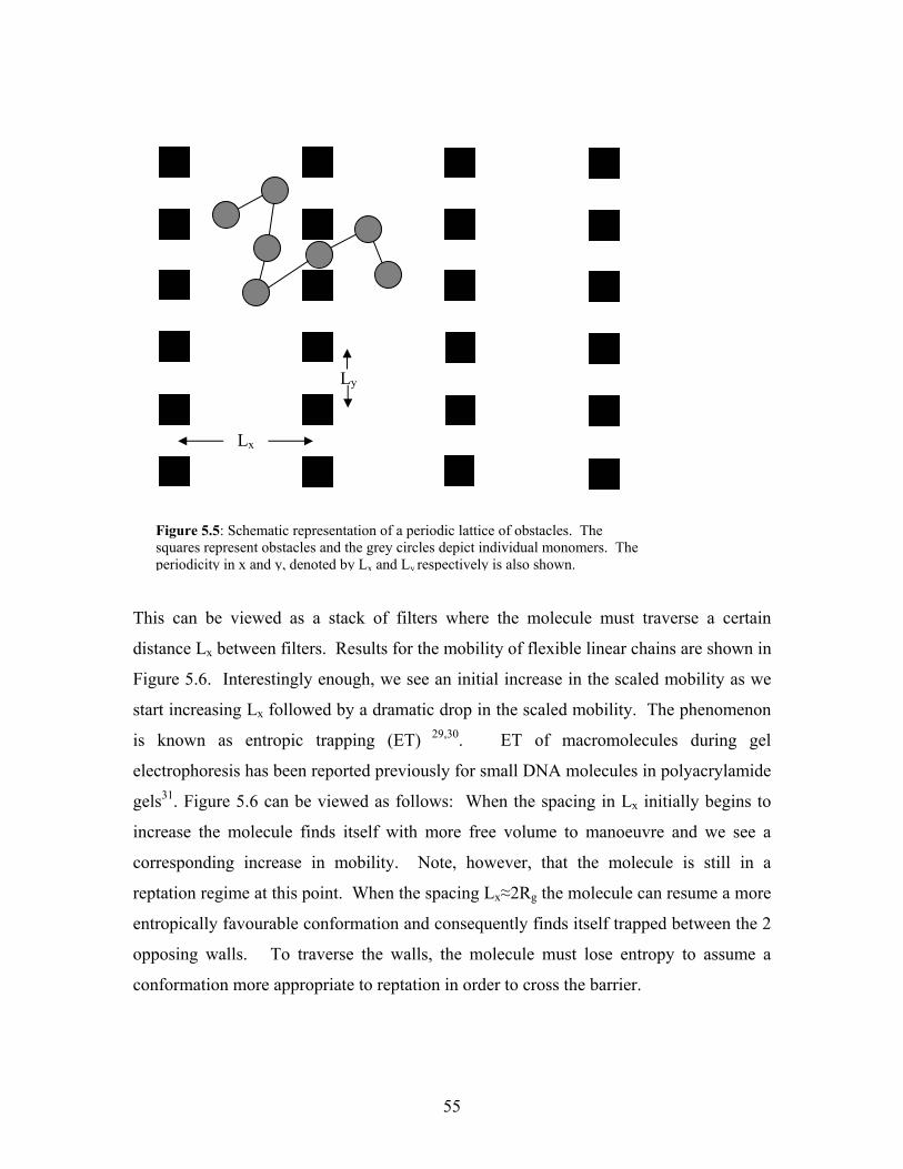
55
This can be viewed as a stack of filters where the molecule must traverse a certain
distance Lx between filters. Results for the mobility of flexible linear chains are shown in
Figure 5.6. Interestingly enough, we see an initial increase in the scaled mobility as we
start increasing Lx followed by a dramatic drop in the scaled mobility. The phenomenon
is known as entropic trapping (ET) 29,30. ET of macromolecules during gel
electrophoresis has been reported previously for small DNA molecules in polyacrylamide
gels31. Figure 5.6 can be viewed as follows: When the spacing in Lx initially begins to
increase the molecule finds itself with more free volume to manoeuvre and we see a
corresponding increase in mobility. Note, however, that the molecule is still in a
reptation regime at this point. When the spacing Lx≈2Rg the molecule can resume a more
entropically favourable conformation and consequently finds itself trapped between the 2
opposing walls. To traverse the walls, the molecule must lose entropy to assume a
conformation more appropriate to reptation in order to cross the barrier.
Ly
Lx
Figure 5.5: Schematic representation of a periodic lattice of obstacles. The squares represent obstacles and the grey circles depict individual monomers. The periodicity in x and y, denoted by Lx and Ly respectively is also shown.
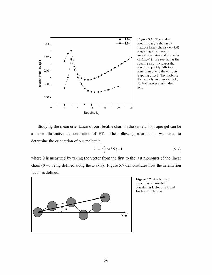
56
0 4 8 12 16 20 24
0.06
0.08
0.10
0.12
0.14
scal
ed m
obilit
y (µ
* )
Spacing Lx
M=3 M=4
Studying the mean orientation of our flexible chain in the same anisotropic gel can be
a more illustrative demonstration of ET. The following relationship was used to
determine the orientation of our molecule:
1cos2 2 −= θS (5.7)
where θ is measured by taking the vector from the first to the last monomer of the linear
chain (θ =0 being defined along the x-axis). Figure 5.7 demonstrates how the orientation
factor is defined.
X=0
Θ
Figure 5.6: The scaled mobility, µ*, is shown for flexible linear chains (M=3,4) migrating in a periodic anisotropic lattice of obstacles (Lx≥Ly=4). We see that as the spacing in Lx increases the mobility quickly falls to a minimum due to the entropic trapping effect. The mobility then slowly increases with Lx for both molecules studied here
Figure 5.7: A schematic depiction of how the orientation factor S is found for linear polymers.

57
An isotropic system gives us S=0 while a molecule predominately oriented along the x
(y) axis would yield values closer to S=1 (S=-1). Figure 5.8 shows our results for the
orientation factor of our flexible chain in a periodic anisotropic gel. As we can see, at
Lx=Ly=4 we have S=0, as expected. Increasing the spacing Lx causes the chain to be
predominately oriented along the y-axis, reaching a minimum orientation value at Lx=7
(S≈-0.14). And, obviously, we have:
0lim =∞→
SxL
(5.8)
Entropic trapping can be viewed as a very effective tool for sieving molecules
according to size since longer chains will require a larger spacing in Lx before trapping
can effectively occur. In fact, our results indicate that it would be possible to have longer
chains elute faster in such a gel than shorter ones. Unfortunately, we could not observe
this in our simulations given the limited size range of our molecules. Another popular
technique for sieving molecules is capillary electrophoresis (including the use of
microchannels). In the next section we will attempt to study this effect by studying the
mobility of molecules in narrow tubes.

58
2 4 6 8 10 12 14 16 18 20 22
-0.15
-0.12
-0.09
-0.06
-0.03
0.00
S=
2<co
s2 (θ)>
-1
periodicity between walls
5.4. Tubes We studied a system based on the principle of capillary electrophoresis. We designed
a narrow channel where our polymer is confined in a narrow tube (Ly=3) of infinite
length. Figure 5.9 shows the lattice used. We expect to see our polymer behave as a
one-dimensional Rouse chain (D~M-α, where α=1). Results are shown in Table 5.3 and
Figure 5.11. A log-log plot of the scaled diffusion constant (D*) vs. molecular mass (M)
reveals a scaling parameter α(M)∼1.41 (Results not shown). This result is higher than
expected but a linear extrapolation of the finite size scaling parameter (eq 4.4) shows that
the value approaches what is expected of a Rouse chain (shown in Figure 5.11). Again,
higher molecular weights will need to be studied before making any definite conclusion
as to the exact value of α. The scaling parameter of the mean square end-to-end distance 2h provides a non-monotonous progression towards the large M limit and we are
Figure 5.8: The orientation factor 1cos2 2 −= θS vs. lattice spacing
Lx for the anisotropic gel system with Ly=4.

59
unable to draw any conclusions as the value of υ(M→∞) from the available results.
Logically, in this case, we would presume that the large M exponent of 2h would be:
∞→→ M|1υ given the one-dimensional aspect of our system (shown below) .
In a second attempt to view ET, we modified the same “channel” by adding obstacles
to create large compartments separated by narrow doors with a small opening. Figure
5.10 shows an example of our gel. The parameters Lx correspond to the length of the
compartment and Ly as its width. The opening is only large enough to permit the passage
of one monomer at a time. Once again, we used flexible linear chains to study this
system. In Figure 5.12 we plotted log(D*) vs. log(M) for various channel lengths Lx.
From Figure 5.12, we see that we have two distinct regimes for the mobility of our
chains. The first is the small M regime where µ~1/Mb, with b>3/2. The scaling
parameter typically associated with ET for large chains are in the range of 3/2<b<3 29-31.
Our results for small chains correspond to these values but more data needs to be
collected to make any firm conclusions about the existence of ET. The second regime is
the large M regime where µ~1/Mc with c<2. In the second regime, we expect the chain to
behave as a one dimensional Rouse chain (D~1/M) and our data seems to be
asymptotically converging towards that result but, once again, more data needs to be
collected to confirm that hypothesis. Therefore, the two regimes correspond to entropic
trapping (small M) and reptation (large M) respectively. We should also mention that to
see any pronounced ET using larger chains we would need to increase the size (Ly>3) of
the gap to allow for our flexible chain to assume its proper ellipsoidal conformation.
(Since the polymer coil is commonly described as a random walk, its shape will not
typically resemble a sphere but rather an ellipsoid because the random walker considers
neither is past nor future. Consequently, the path described by the polymer coil will tend
to explore an area rather thoroughly before moving on to the next area. This causes
Ly=3
Figure 5.9: Schematic representation of a polymer confined in a two-dimensional tube

60
anisotropy in the shape of the polymer that makes it look like an ellipsoid as opposed to a
sphere.)
Table 5.3: Flexible Chain in a narrow tube
LEGEND: M=# of monomers, D=Diffusion Coefficient, 2h =end-to-end distance, α(M)=scaling
exponent of D, υ(M)=scaling exponent of 2h M D Number of
conformations 2h α(M+½ ) ν(M+½ )
2 0.077381 42 7.3810 1.5427 1.12465 3 0.041398 396 18.3737 1.44092 1.18462 4 0.027350 3 224 36.3251 1.29223 1.25483 5 0.020499 24 588 63.5943 1.20643 1.22226 6 0.016451 186 120 99.3068 ∞ 0.95 ± 0.08 N/A
0.0 0.1 0.2 0.3 0.40.90
0.95
1.00
1.05
1.10
1.15
1.20
1.25
1.30
1.35
1.40
1.45
1.50
1.55
1.60
α(M
+1/2
)
1/(M+1/2)
Ly=3 Lx
Figure 5.11: Diffusion scaling exponent α of a flexible polymer in a narrow tube (Ly=3). We see that the linear extrapolation yields near Rouse-like dynamics from the arrow extending the linear fit.
Figure 5.10: Schematic representation of a polymer in a tube with obstacles that serve as entropic traps.

61
0.2 0.3 0.4 0.5 0.6 0.7 0.8 0.9 1.0
-3.0
-2.8
-2.6
-2.4
-2.2
-2.0
-1.8
-1.6
-1.4
-1.2
0.2 0.3 0.4 0.5 0.6 0.7 0.8 0.9 1.0
-3.0
-2.8
-2.6
-2.4
-2.2
-2.0
-1.8
-1.6
-1.4
-1.2
-1.0
0.2 0.3 0.4 0.5 0.6 0.7 0.8 0.9 1.0
-2.5
-2.0
-1.5
0.2 0.3 0.4 0.5 0.6 0.7 0.8 0.9 1.0
-2.5
-2.0
-1.5
A
-1.45
-3.79
log
(D* )
log (M)
Lx=4
-1.52
-4.05
B
log(
D* )log (M)
Lx=5
-1.16
-1.98
C
log(
D* )
log(M)
Lx=6
-1.09
-1.78
D
log
(D* )
log(M)
Lx=7
Figure 5.12: Log (µ*) vs Log (M) for the tunnel system (Fig. 5.10). Lattice spacings are: Lx=4 (A), Lx=5 (B), Lx=6 (C) and Lx=7 (D). Power law fits µ*~Mh are shown, and the exponents h are given.

62
Chapter 6
Discussion In this section we globally discuss our results in general terms in hopes of gaining a
big-picture perspective of what was achieved in this thesis. We will start with a synopsis
of what has been achieved and review the goals set forth at the beginning of this project.
We will then discuss the importance of the OMRC model despite our findings that it may
lead to erroneous assumptions.
In chapters 2 to 6 we successfully improved an existing model and were able to
properly simulate the behaviour of various molecules in solution. With the exception of
the star chains, all our results correspond to expected results. More importantly, we were
able to find proper results without having to resort to stochastic algorithms. This is
significant since we achieved better results in a fraction of the time it would take for, say,
Lattice Monte Carlo simulations.
The first part of this thesis focussed on the exactness of our data and this focus paid
off. We uncovered the extent to which entropic trapping can be useful in separating
molecules. One of the goals of this thesis was to have smaller molecules diffuse more
slowly than larger ones using the right sieving gel. Unfortunately, we were never able to
achieve this but we are confident that it is still a possibility using larger molecular sizes
and appropriate entropic trapping gels. Several papers have subsequently found a use for
entropy using micro fabricated devices. Meller and Branton32 studied diffusion of linear
polymers through a channel and reported that the most probable time of passage, τp,
follows two regimes: One for small molecular sizes and one for larger one. The transition
between regimes seemed to be heavily influenced by the length of the entropic channel
(which in this case was a single passage). We also identified two regimes based on the
size of the molecule with regard to diffusion of linear polymers in tubes separated by
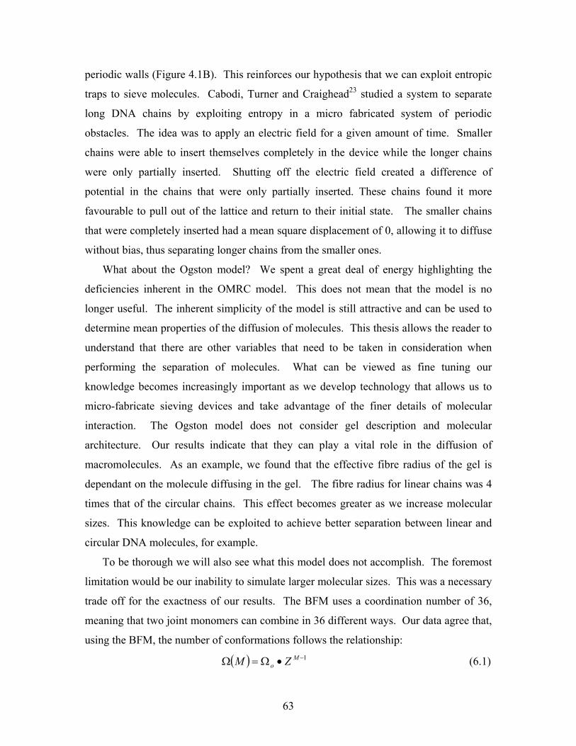
63
periodic walls (Figure 4.1B). This reinforces our hypothesis that we can exploit entropic
traps to sieve molecules. Cabodi, Turner and Craighead23 studied a system to separate
long DNA chains by exploiting entropy in a micro fabricated system of periodic
obstacles. The idea was to apply an electric field for a given amount of time. Smaller
chains were able to insert themselves completely in the device while the longer chains
were only partially inserted. Shutting off the electric field created a difference of
potential in the chains that were only partially inserted. These chains found it more
favourable to pull out of the lattice and return to their initial state. The smaller chains
that were completely inserted had a mean square displacement of 0, allowing it to diffuse
without bias, thus separating longer chains from the smaller ones.
What about the Ogston model? We spent a great deal of energy highlighting the
deficiencies inherent in the OMRC model. This does not mean that the model is no
longer useful. The inherent simplicity of the model is still attractive and can be used to
determine mean properties of the diffusion of molecules. This thesis allows the reader to
understand that there are other variables that need to be taken in consideration when
performing the separation of molecules. What can be viewed as fine tuning our
knowledge becomes increasingly important as we develop technology that allows us to
micro-fabricate sieving devices and take advantage of the finer details of molecular
interaction. The Ogston model does not consider gel description and molecular
architecture. Our results indicate that they can play a vital role in the diffusion of
macromolecules. As an example, we found that the effective fibre radius of the gel is
dependant on the molecule diffusing in the gel. The fibre radius for linear chains was 4
times that of the circular chains. This effect becomes greater as we increase molecular
sizes. This knowledge can be exploited to achieve better separation between linear and
circular DNA molecules, for example.
To be thorough we will also see what this model does not accomplish. The foremost
limitation would be our inability to simulate larger molecular sizes. This was a necessary
trade off for the exactness of our results. The BFM uses a coordination number of 36,
meaning that two joint monomers can combine in 36 different ways. Our data agree that,
using the BFM, the number of conformations follows the relationship:
( ) 1−•Ω=Ω Mo ZM (6.1)

64
Table 6.1 shows our data fits using various molecules in different gel systems. It is
possible to use a lattice description that has a much lower coordination number and allow
us to study molecular sizes as large as M=10 in solution, or M~15 when introducing
obstacles. Unfortunately, this still falls in the realm of very small molecular sizes.
Heudkelum, Barkema and Bisseling34 were able to study reptation dynamics of chains up
to M=15 exploiting symmetries in polymer conformations and using parallel processing
for computation. The coordination number used was Z=6 in 3D and they limited
molecular dynamics to the reptation regime.
Table 6.1: # of Conformations: ( ) 1−•Ω=Ω Mo ZM
Molecule/Lattice Ωo Z Flexible chain/solution 1.34 27.84 Circular chain/solution 0.85 14.41 Stiff chain/solution 3.40 10.57 Flexible chain/ periodic array of obstacles (Lx=Ly=4)
9.73 9.48
A common theme throughout this first part of the thesis is that we make
extrapolations that are based of just a few points. The results of our extrapolations
indicate that the study of larger molecules using this exact model will provide very good
results. Unfortunately, a common goal in the study of polymer physics is to develop
universal relationships. Given the small range of molecular sizes that we studied, it is
unreasonable to make any type of universal assertions. Along those same lines, certain
extrapolations that were presented can be viewed as dubious since they are made using
only 2 or 3 data points. Examples of this are found throughout this work. The fact that,
in several instances, our extrapolations come very close to theoretically accepted results
offers credulity to our methodology even if results were obtained using minimal data.
65
PART II
Chapter 7
Anomalous Diffusion 7.1 Introduction In Part II of this thesis, we study the displacement of a particle in various media
impeding the particle’s movement, or more precisely, its mobility (if a net external field
is applied) and diffusion. Most works concentrate on the long-term effects or steady state
solutions and emphasis is rarely made to study the short-term effects. How does a
particle achieve a steady state? How fast does it achieve this state? Which factors affect
the particles ‘journey’ to a steady state? Is this transient regime something that can be
observed? Can it be exploited in new separation devices? All of these questions lead us
back to the OMRC model and its inability to describe short-term effects due to
inhomogeneity of the medium and the anisotropy of the system caused by the presence of
an external electric field. For example, it was reported39,40 that gels with fractal
geometry41 are much more effective at trapping particles in dead-ends than homogeneous
random gels. An experimental study conducted by Sturm et al.16 was presented to
ascertain the dynamic behavior of latex beads in an agarose gel whose concentration
ranged from 0.6% to 1.4%. Specifically, it was a study of the short-time scaling behavior
of the particle’s mean square displacement. Therefore, it seems appropriate to investigate
these same issues using a theoretical model and to compare our results to those of Sturm
et al.16. In Part II, we will use an exact enumeration method to follow and characterize
the displacement of a particle at various time intervals using a variety of obstacle

66
distributions. In Section 7.2, we will discuss the relevant theory while Section 7.3
introduces the numerical model we will be using.
7.2 Theory Normally, the steady state diffusion of an analyte follows a linear regime with time, t
(eq 1.4):
( ) tdDtr o22 = (7.1)
where d is the dimensionality, Do is the diffusion constant and ( )tr 2 is the mean square
displacement. In the short time regime, on the other hand, we often find that ( )tr 2 is
not a linear function of time because the analyte has not had sufficient opportunity to
fully explore its surroundings. The phenomenon is even more pronounced when the
particle moves in a fractal environment. This is rarely a typical experimental situation,
however, since the fractality of all real systems are limited both at the small and large
length scales. The short-time anomalous diffusion regime can often be described by the
scaling law:35-37
( ) wdtdDtr2
*2 2 ⋅= (7.2)
where dw is the fractal dimension of the walk and is usually greater than 2 due to the
possibility of the particle being impeded within the lattice. The term fractal dimension is
a misnomer. It makes reference to the initial belief that anomalous diffusion can only be
observed in the diffusion of particles in a fractal gels. We will show in this second part
that anomalous diffusion can be observed regardless of whether the distribution of
obstacles is fractal or not. Also, D* is the effective anomalous diffusion coefficient,
valid for the transient regime only. Sturm et al.16 found that dw was independent of the
gel concentration in the absence of an electric field (within error bars). Moreover, Sturm
et al.16 found that the mean square displacement of the particles scales less than linearly
with time when no electric field was applied (dw>2). This result indicated that the
agarose gel is indeed a fractal36,37(at least over the length scales probed by their
experimental system) whose structure is independent of gel concentration. These results

67
are shown in Figure 7.1. Comparing eq (7.1) and eq (7.2) we get the transition time
solving:
*
12
2*22
DD
t
tdDtdD
od
do
w
w
=
=
− (7.3)
or,
w
wd
d
oss D
Dt
−
=
2
* (7.4)
where tss is thus the time of transition between short-time and the steady state diffusion of
particles. Equivalently, substituting eq (7.4) into eq (7.1) we obtain:
ssoss tdDr 2= (7.5)
where rss is the distance at which the transition to steady-state motion of particles will
take place within the system. A system may thus look fractal over length (time) scales
shorter than rss (or tss), and normal otherwise.
Theory holds that an applied field will add a term to eq (7.1). Hence we have16:
( ) 222 6 tvDttr +≈ (7.6)
where v is the mean drift velocity. So far, we have only expressed the movement of
particles in terms of ( )tr 2 . Slater, Guo and Gauthier42,44 have reported that the addition
of an electric field creates an anisotropy in the system causing a difference in the
transverse and longitudinal diffusion constants. To study this anisotropy, we will thus
define the electric field along the x-axis and study the first and second moments of the
displacement in each Cartesian direction. We then have:
( )
( ) ( )
( ) ( )( )dt
txtxdD
ttttxtx
tvtx
tx
d
x
w
22
ss
222
lim21
.for ,
−=
<∝−
=
∞→
(7.7)

68
where ( )tx is the drift of the particle along the x-axis and the
variance ( ) ( ) 22 txtx − behaves as a pure diffusive process for times t>>tss43. The above
equations are equivalent in the y,z-directions with vy=vz=0. In contrast to the field-free
experiments, the value of dw was smaller in the presence of an electric field (10V/cm)
using the same gel. Moreover, dw was an increasing function of the gel concentration.
Figures 7.1 and 7.2 show these results. On the one hand, while the bead is moving
within a gel pore, its dynamics are governed by a drift process (2nd term of eq. 7.6). On
the other hand, once the bead collides with a gel fiber, the bead movement is impeded by
the field pushing the bead against the gel strand. As the concentration increases, the time
between collisions shortens and the bead dynamics are predominantly governed by
collisions (hence by random processes). Consequently, at low concentrations, we expect
the particle’s movement to be dominated by the second term of eq. (7.6) (i.e. drift
process). At higher concentrations, the combination of increased collisions and the
electric field pushing the particle against the gel strands causes the particle’s overall
dynamics to be dominated by a diffusion-like process. This explains why values of dw<2
were obtained for low concentrations and an increase in dw was observed as the
concentration increased.
Using the theoretical elements presented in this section, we will be able to use our
theoretical model to characterize the anomalous diffusion of particles and compare our
results with those found in ref [16]. The next section will introduce the model used to
study the motion of particles on short time scales.

69
Figure 7.1: Results of Ref [16], showing 2/dw vs. gel concentration. The following legend is used: x direction,
E=10V/cm y direction
E=10V/cm x direction
E=0 y direction
E=0

70
7.3 The model As mentioned before, this model will involve an exact enumeration of all particle
trajectories. Using a cubic lattice in 3D, we enumerate all these trajectories of the
particle based on an initial starting point. We can compute probabilities associated with
each trajectory and derive ( ) ( )txtx 2 and (or ( ) ( ) ( ) ( )tztztyty 22 , and , ) for a
given time t. Taking an averaging over all initial conditions (weighted equally) we can
determine those values exactly. To illustrate this exact enumeration approach, Figure 7.3
shows a simple unbiased diffusion problem in 2 dimensions on a lattice without
obstacles:
Figure 7.2A: Results of ref [16] showing the first moment of the mean displacement in the x and y directions vs. time with an applied external field of 10V/cm applied in the x-direction. The lines represent the best linear fit of the data.
Figure 7.2B: Results of ref [16] showing the second moment of the mean displacement in the x and y directions vs. time with an external field of 10V/cm applied in the x-direction. The lines represent the best linear fit of the data.

71
In three dimensions, the probabilities for jumping are given by:
61
=== ±±± zyx ppp (7.8)
The general expression for the probability of presence nxyz(t) on site (x,y,z) at time t is
given by the equation:
( ) ( ) ( ) ( ) +−+−+−= +−−++− yzyxxzyxxzyxxyz ptnptnptntn 111 ,1,,,1,,1 (7.9)
( ) ( ) ( ) zzyxzzyxyzyx ptnptnptn −−+−−+ −+−+− 111 1,,1,,,1,
Using this method we also have the luxury of introducing an electric field (or another
driving force) by modifying the probabilities of transition accordingly. We will use the
same approach discussed in section 2.2. Hence,
εε
ε
−+
±
± +⋅=
eeep x 3
1 (7.10)
Figure 7.3: We show the unbiased distribution of probabilities of a particle in 2D at times t= 0, 1, 2, and 3.

72
where ε is the scaled field defined by eq (2.8). The probabilities in the ±y,z directions
remain unchanged and are given as follows:
61
== ±± zy pp (7.11)
Unlike the model described in chapter 2, this model does not strictly define the electric
field as ‘vanishing’. Therefore, we can choose stronger values of the electric field in our
study. That being said, however, our intent is to learn of the short time dynamics of
particles and is not a study of the drift velocity. Hence, we will be keeping the value of
the electric field relatively small.
The presence of obstacles will, of course, affect the distribution of probabilities and
we need to define a methodology for treating obstacle interactions with regard to the
model: If a move leads to a lattice site containing an obstacle, the move is rejected and
the probability of moving towards the obstacle is then applied to the particle’s initial
location on the lattice. This is standard in Monte Carlo simulations.
The short time dynamics of a particle is incumbent upon many parameters. Foremost
of which is the nature of the obstacles and their distribution. The presence alone of
obstacles may cause anomalous short-time dynamics but if the concentration of obstacles
is small we expect that this effect will be negligible. When the concentration approaches
the percolation limit we expect that the anomalous diffusion will be more prevalent.
Finally, when the array of obstacles becomes fractal we can argue that the particle never
reaches a state of steady motion because the correlation length of the fractal aggregates
diverges, and the long term anomalous diffusion exponent dw would scale to a factor
larger than 2. The extent to which the diffusion is anomalous will likely depend on the
fractal dimension of the obstacle distribution and the length scale over which this fractal
nature applies. We will also investigate how the application of an external field affects
the short-term dynamics of particles. Chapter 8 will focus on validating our model by
studying various lattice systems with and without an applied external field.

73
Chapter 8
Anomalous Diffusion:
Results
8.1 Validation of the model (ε=0) The first step is to verify the enumeration method in the unbiased (no external field)
limit to make certain that it yields proper values of the diffusion constant for long times.
We will start with a particle in solution (no obstructions) and follow through with simple
periodic obstruction schemes. We will compare our values with those found in the
literature to validate our method.
We will start with a particle in free solution. Mercier and Slater13 devised an exact
method of extracting the steady-state diffusion constant of an analyte in 3 dimensions.
We will be using results found in that paper as a basis for our comparison. We expect the
diffusion process to follow the scheme in eq (7.1). The diffusion coefficient of a particle
in free solution is expected to be D=1/6 if we use our notation and dimensionless units.
The results of our simulations using the model presented in Section 7.3 provide identical
values of the diffusion constant (shown in Figure 8.1). Of note is the fact that there is no
transient to the steady-state diffusion constant. This means that the transition to a steady
state regime is only non-trivial when obstacles are present. This is an expected result.

74
0 2 4 6 8 100.00
0.05
0.10
0.15
0.20
0.25
0.30
0.35
0.40
D=<
R2 (t)>/
(6*t)
Time, t
Our results for ( )tx 2 and ( )ty 2 are shown in a different way in Figure 8.2. We
see that in the absence of obstacles and external biases the components are equivalent,
i.e., the system is isotropic for all times 0≥t . Furthermore, the slope is 1 which indicates
that the diffusion coefficient is constant (see eq (7.1)) and that there is no transient
behavior. This was also expected. Moreover, from eq. 7.1, we have:
( )[ ] ( ) )2log(loglog 2 dDttx += (8.1)
which implies that the intercept on the vertical axis should be: 4771.0)2log( −=dD (by
substituting the values d=1 and D= 61 ). In Figure (8.2), we see the plot of eq (8.1) and
find that both slope and y-intercept confirm the fact that there is no transient behavior.
Figure 8.1: Diffusion of a particle in solution (no obstacles) and without bias (ε=0). The solid line represents the steady state solution D=1/6.

75
0.0 0.2 0.4 0.6 0.8 1.0-0.6
-0.4
-0.2
0.0
0.2
0.4
0.6
1
log(<x2(t)>)=log(t)+log(1/3)
log[
<X2 (t)
>]
log
[<Y2 (t)
]
log(time)
We thus conclude that in the absence obstacles, our model provides the expected
(trivial) results. The addition of obstacles in our lattice will cause the particle to undergo
a transient regime where the mean square displacement will not scale linearly with time.
Before presenting our results it would be useful to discuss how the values of D*, Do and
dw are going to be computed. After running several test simulations on a variety of
periodic lattices it became quite clear that, in most cases, the transition from an
anomalous diffusive regime to the steady-state regime is done smoothly and we generally
have:
2→wd as ∞→t (8.2)
Although we knew to expect such a transition we did not anticipate its smoothness. The
value of dw was found by taking consecutive slope values of eq (7.2). In other words,
from eq. (7.2), we have:
( ) wdtdDtr2
*2 2= (8.3A)
( )( ) ( ) ( )td
dDtrw
log22loglog *2 += (8.3B)
( ) ( )( )( )( ) )log(1log
log1log222
1,tt
trtr
dttw −+
−+=
+
(8.3C)
Figure 8.2: Log-log plot of the unbiased (ε=0) mean square displacement vs. time of a particle in solution (no obstacles). We see that both components overlap (the points are absolutely identical) and that the slope is 1, as expected.

76
( )( )
[ ]t
trtr
dttw 11log
1log
22
2
1, +
+
=
+
(8.3D)
From eq. (8.3D), we can easily find the “instantaneous” value of dw for all times t.
Equivalently, we can express eq. (8.3D) in terms of its component in x,y and z. This
becomes necessary when an external field is applied because the effective fractal
dimension, dw, may then be different for each Cartesian coordinates. In fact, we would
have to study the components dw,x, dw,y and dw,z of the fractal dimension for the study of
anisotropic gels. Using the second moment of displacement (eq 7.7) to determine the
value of the fractal dimension of the particle, we will effectively factor out the particle
drift to study the particle’s diffusive properties. To avoid confusion, we will use the
notation: (dw,x, dw,y, dw,z) to distinguish which component of the fractal dimension we are
studying.
Figure (8.3) shows how dw,x evolves for a lattice of periodic obstacles while Figure
(8.4) shows the same graph for a lattice of infinitely long periodic fibers.
0 2 4 6 8 10 12 14 162.001
2.002
2.003
2.004
2.005
2.006
2.007
2.008
2.009
Anom
alou
s Ex
pone
ntd w
,x
time
In a lattice of periodic obstacles, we observe how dw,x monotonously transitions to its
steady state value (dw,x=2), in accordance with eq (8.2). We also note that at t=4 we see
a slight kink in the value of dw,x which corresponds with the obstacle’s periodicity (P=4).
Figure 8.3: Anomalous exponent dw,x vs. time in a lattice of periodic obstacles with an obstacle periodicity, P=4 (shown on the right). The steady-state value is
0.2|, =∞→txwd

77
Since the gel architecture is uniform in all Cartesian coordinates and no external field is
applied we have:
wzwywxw dddd === ,,, (8.4)
In Figure (8.4) we see quite a different picture for the evolution of dw,x vs. time: the value
of dw,x reaches a maximum value before resuming a monotonous decrease towards the
steady-state value. The value of dw,x shown here and in Fig 8.3 is always subdiffusive
(dw>2). This is consistent with the findings of Starchev et al.16 for the short-time
displacement of a particle in the absence of an applied field (see our Fig. 7.1). The
central question of this chapter is whether we will observe any superdiffusion effects
when a field is applied. This will be investigated in the next section. We also observed a
direct correlation between the periodicity of the lattice and the time at which the
maximum value of dw,x is reached. In Figure 8.5A, we see the anomalous exponent, dw,x,
vs. time, t for a particle in a lattice of infinitely long periodic fibres (ε=0) for several
periodicities, P. We see that in most instances, the value of dw,x reaches a maximum
value before making the transition described in eq. (8.2) (the only exception is for P=3
where the value of dw,x starts at a local maximum value). We will call the time at which
this maximum value is reached tmax. In Figure (8.5B) we see a plot of tmax vs. P. Except
for P=3 (this case has 2 maxima), the relationship between tmax and P is linear and exactly
depicted by the following relationship:
3P ,2max >+= Pt (8.5)
0 5 10 15 20 25 30 35 40 45
2.02
2.03
2.04
2.05
2.06
2.07
2.08
2.09
d w,x
time
Figure 8.4: Anomalous diffusion exponent dw,x vs. time for a lattice of infinitely long periodic fibers. The periodicity in this example is P=4 (the lattice is shown on the right with P=9 for clarity). The value of dw,x reaches a maximum before making a monotonous transition to its steady-state value, dw=2.

78
0 2 4 6 8 10 12 14 16 18 20 22 24 26 28 30 32
2.02
2.04
2.06
2.08
2.10
2.12
2.14 P=3 P=4 P=5 P=6 P=7
anom
alou
s ex
pone
ntd w
,x
time, t
3 4 5 6 71
2
3
4
5
6
7
8
9
10
t max
Periodicity, P
Given the various ways in which dw can evolve in time, we are faced with having to
choose a definition of dw which will be used for all systems. To ensure consistency, we
will always choose dw based on the slope of the first 2 times (dw|t=1,2). In other words, we
use eq. (8.3D) using times t=1,2. Consequently, the value of D* will be found by finding
the y-intercept of eq. (8.3B), using only times t=1,2. We illustrate how this is
accomplished in Figure (8.6).
Figure 8.5A: Anomalous diffusion exponent, dw,x vs. time in a lattice of infinite periodic fibers (ε=0) for several periodicities, P. The vertical lines depict the point at which the maximum value of dw,x is obtained.
Figure 8.5B: tmax vs. Periodicity in a lattice of periodic infinite fibers (ε=0). Here, tmax is defined as the time at which the anomalous exponent dw reaches a maximum. We see that after P=3, we have a linear progression of tmax. The linear fit represents the expression:
Pt += 2max

79
Note that we also define the “current” diffusion coefficient ( ) trtD 62= . By
definition, we expect:
( ) ∞→→ tDtD o as (8.5)
0.0 0.2 0.4 0.6 0.8 1.0 1.2 1.4 1.6
-0.2
0.0
0.2
0.4
0.6
0.8
1.0
1.2
1.4
log(<r2(t)>)=-0.09691+0.9386*log(t)log(
<r2 (t)
>)
log(t)
To find the value of the steady-state diffusion constant Do we have two options: The first
was already mentioned and that is to take values of the exact steady-state diffusion
constant (Do=0.1309799) found in ref [37]. The second option is to graph the current
diffusion coefficient D(t) against t1 . Since D(t) is defined as the time evolution of the
diffusion coefficient to its steady-state value, we can extrapolate the two values of D(t)
corresponding to the highest times to find a reasonable approximation of the steady-state
diffusion constant, Do, by taking the y-intercept. In Figure 8.7A, we test this
methodology using a lattice of infinitely long fibers. The thin solid line represents the
linear extrapolation while the thick horizontal solid line is the actual steady state value
reported in ref [37]. Surprisingly, the value found using the linear extrapolation is
exactly the steady-state value reported in ref [37] (to the 7th decimal). In fact, taking a
linear extrapolation of D(t) using t= 30...40 reproduced the value of the Do to the same
precision!! This result shows that after a certain time, D(t) approaches its steady-state
value linearly. We suspect that this transition time is strongly linked to the periodicity of
the system. In Figure 8.7B, we test this linear relationship by plotting (D(t)-Do) vs. (1/t).
If the progression of D(t) towards Do is indeed linear, the slope of the resulting log-log
Figure 8.6: We illustrate the manner in which the value of D* is found. The results shown are for a particle in a lattice of infinite periodic fibres (P=3, ε=0). The equation shown is taken from eq. (8.3B) and the slope is given by eq. (8.3D). The linear extrapolation used to find D*is done using times t=1, 2. In this case, D*=10-0.09691=0.13333 and 2/dw=0.9386.

80
plot should be 1. The linear fit shown in Figure 8.7B is accomplished using the last 3
points. We see that the value of the slope is indeed very near unity indicating a linear
convergence: 1.for )( >>+= ttADtD o
0.0 0.2 0.4 0.6 0.8 1.00.130
0.135
0.140
0.145
0.150
D(t)
1/t
-1.6 -1.4 -1.2 -1.0 -0.8 -0.6 -0.4 -0.2 0.0 0.2-3.0
-2.5
-2.0
-1.5
-1.0
m=0.999
89(2)
log(
D(t)
-Do)
log(1/t)
In this section we presented basic results that were designed to validate the model and we
provided details on how we extract the values of dw, D* and Do. We showed that in the
absence of obstacles there is no transient behavior of the diffusion constant. We also
Figure 8.7A: The unbiased short time diffusion constant, D(t) vs.
t1 in a lattice of infinite periodic fibers (P=4). The black squares represent D while the thin solid line is the linear extrapolation of the last 3 points (D at t=38-40). The extrapolation reveals:
( )213098000.0|)( =∞→ttD The thick horizontal solid line represents the exact steady state value (Do=0.13097999) reported in ref [37].
Figure 8.7B: Log-log plot of (D-Do) vs. 1/t. The slope m~1 indicates that the progression of D to Do does indeed become linear after a certain time. This greatly facilitates the calculation of the steady-state value Do in cases where no exact result exists.
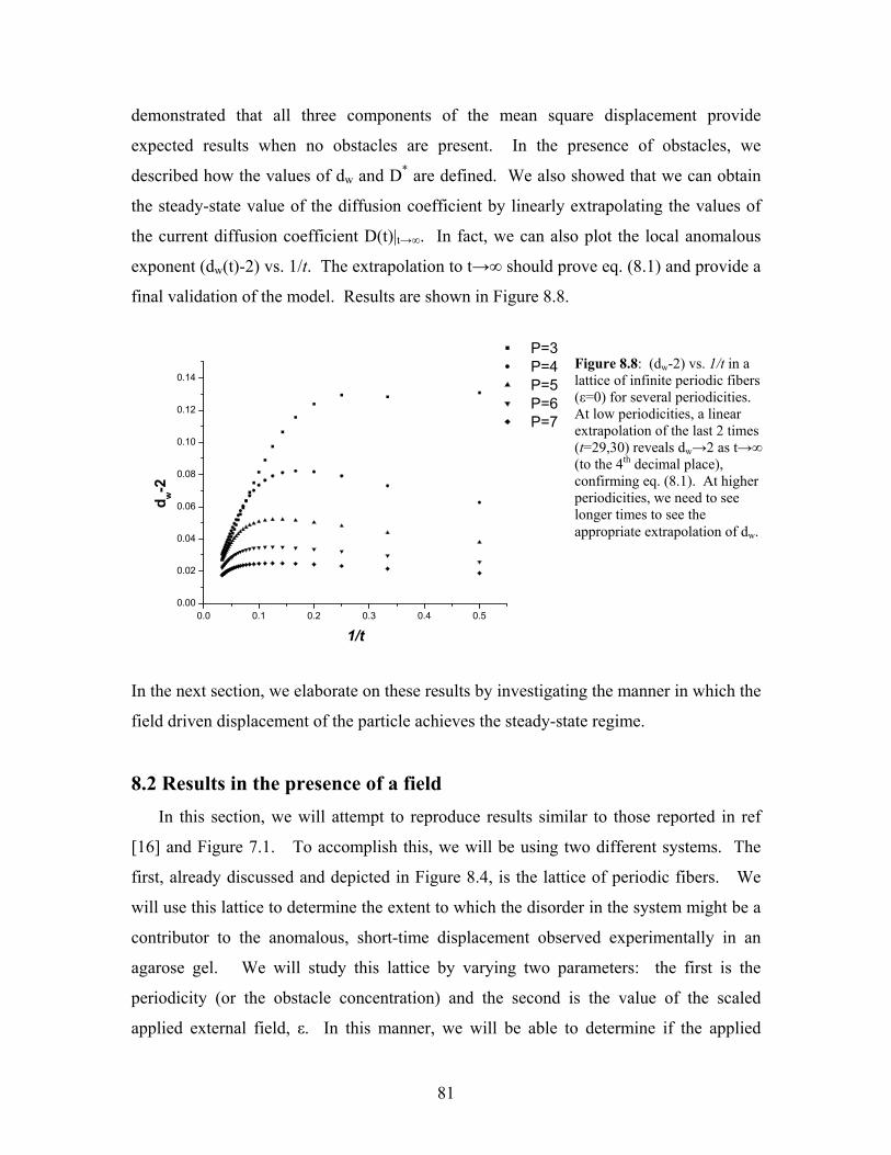
81
demonstrated that all three components of the mean square displacement provide
expected results when no obstacles are present. In the presence of obstacles, we
described how the values of dw and D* are defined. We also showed that we can obtain
the steady-state value of the diffusion coefficient by linearly extrapolating the values of
the current diffusion coefficient D(t)|t→∞. In fact, we can also plot the local anomalous
exponent (dw(t)-2) vs. 1/t. The extrapolation to t→∞ should prove eq. (8.1) and provide a
final validation of the model. Results are shown in Figure 8.8.
0.0 0.1 0.2 0.3 0.4 0.50.00
0.02
0.04
0.06
0.08
0.10
0.12
0.14
P=3 P=4 P=5 P=6 P=7
d w-2
1/t
In the next section, we elaborate on these results by investigating the manner in which the
field driven displacement of the particle achieves the steady-state regime.
8.2 Results in the presence of a field In this section, we will attempt to reproduce results similar to those reported in ref
[16] and Figure 7.1. To accomplish this, we will be using two different systems. The
first, already discussed and depicted in Figure 8.4, is the lattice of periodic fibers. We
will use this lattice to determine the extent to which the disorder in the system might be a
contributor to the anomalous, short-time displacement observed experimentally in an
agarose gel. We will study this lattice by varying two parameters: the first is the
periodicity (or the obstacle concentration) and the second is the value of the scaled
applied external field, ε. In this manner, we will be able to determine if the applied
Figure 8.8: (dw-2) vs. 1/t in a lattice of infinite periodic fibers (ε=0) for several periodicities. At low periodicities, a linear extrapolation of the last 2 times (t=29,30) reveals dw→2 as t→∞ (to the 4th decimal place), confirming eq. (8.1). At higher periodicities, we need to see longer times to see the appropriate extrapolation of dw.

82
external field has a significant impact on the effective anomalous scaling exponent. The
second lattice studied simulates a succession of periodic traps. The obstacles are placed
in a way that will effectively impede the movement of the particle in the direction of the
external field. This lattice will be depicted in Figure 8.12
8.2.1 Periodic Fibres Results for a lattice of infinite periodic fibers in the absence of an electric field have
already been presented while testing the validity of the model (Figures 8.4-8.8). With
ε=0, we actually had the trivial results (not shown):
( ) 2222
0
zyxxx
zyx
===−
=== (8.6)
These relations are intuitive and expected. With the application of a field, eq (8.6) no
longer applies. In Figure 8.9 we show our results with ε=0.38.
-0.2 0.0 0.2 0.4 0.6 0.8 1.0 1.2 1.4 1.6
-0.6
-0.4
-0.2
0.0
0.2
0.4
0.6
0.8
1.0
1.2
m~0.985(
1)
m~0.939
(3)
m~1.44
8(3)
m~0.99(
1)
log(
<x2 >)
, log
(<y2 >)
log(time)
Figure 8.9A, shows the mean displacement along both the x and y-axis. Once averaged
over all initial conditions, the data provide a constant value of the velocity in the x-
direction while showing no bias in the y-direction (ie: 0=y ). Equivalently, we also
0 5 10 15 20 25 30
0.0
0.5
1.0
1.5
2.0
2.5
<X>,
<Y>
time
Figure 8.9A: The mean displacement of a particle against time in a lattice of periodic and infinitely long fibers (P=3) with an applied field parallel to the x-axis (ε=0.38). The squares represent the movement along the x-axis while the circles show the movement along the y-axis.
Figure 8.9B: Log-log plot of the mean square displacement of a particle vs. time in a lattice of periodic and infinitely long fibers (P=3) with an applied field parallel to the x-axis (ε=0.38). The squares represent the movement along the x-axis while the circles show the movement along the y-axis.

83
have 0=z (results not shown). The results of Figure 8.9A are equivalent to those
obtained by Sturm et al. [16] (see our Figure 7.2). In Figure 8.9B, we show a log-log plot
of the mean square displacement against time in both the x and y directions. Recall that
the value of the slope, m, is given by wdm 2= in the zero field limit. In the y-direction,
we see a sub-linear scaling parameter for short times that slowly makes the transition to
the expected linear regime (ie: 12 , =ywd ). The results for the movement in the y-
direction are consistent with those found in the previous section (ε=0) since the applied
external field is perpendicular to the y-axis and should not directly affect displacement in
that direction. In the x-direction, however, our results are consistent with eq (7.6) and
Figure 8.9A. The initial scaling is close to unity and steadily increases with time,
showing a value of m≅ 1.45 at times t=29,30. For larger times, we expect that the scaling
of the mean square displacement, 2x will reach the asymptotic value of m=2, as
predicted by eq (7.6) (the drift regime). While Starchev et al. [16] reported an elaborate
interplay between drift and trapping, we don’t observe this using a lattice of periodic
fibers. This is not a very surprising result since an ordered, periodic lattice is not
expected to generate any trapping mechanism (e.g., dead-ends). We also plotted the
second moment of the displacement in both the x and y-directions. Results are shown in
Figure 8.10.
-0.2 0.0 0.2 0.4 0.6 0.8 1.0 1.2 1.4 1.6-0.8
-0.6
-0.4
-0.2
0.0
0.2
0.4
0.6
0.8
1.0
log(
<X-<
X>>2 ),
log(
<Y-<
Y>>2 )
log (time)
Figure 8.10: The second moment of the displacement in both the x and y directions for a particle in a lattice of periodic fibres (P=3) in the presence of an external field (ε=0.38). The line represents the second moment in the x-directions while the points show the second moment in the y-direction.
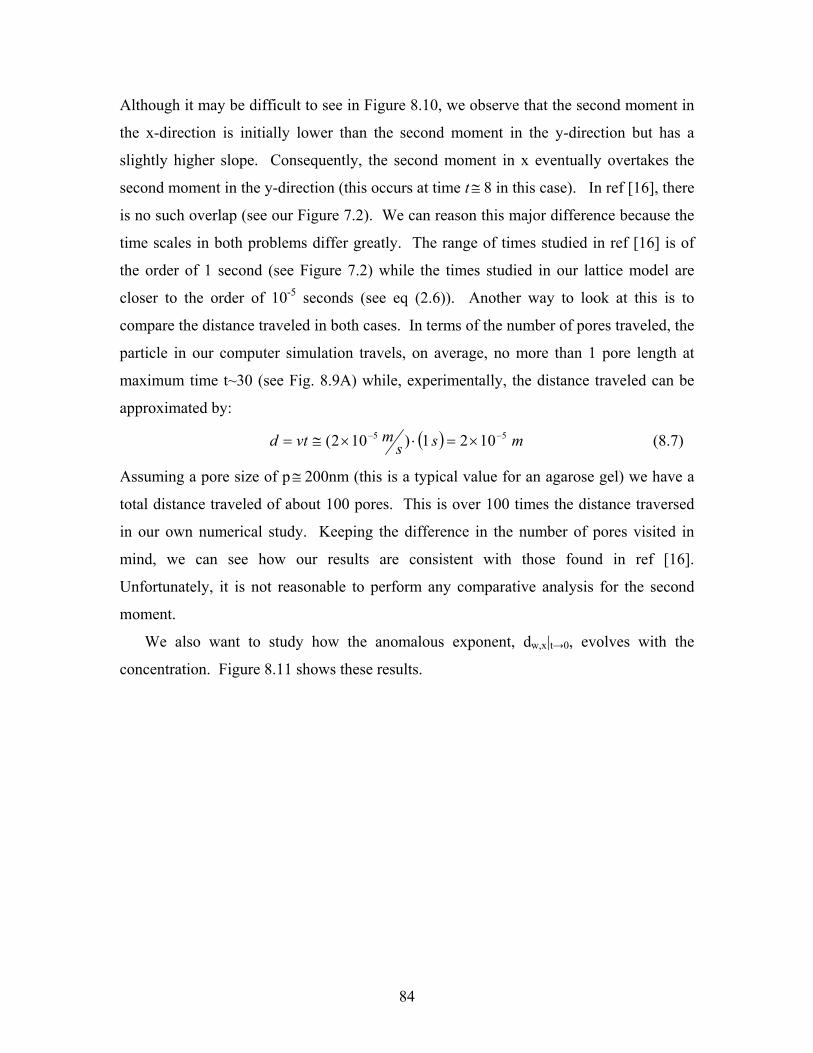
84
Although it may be difficult to see in Figure 8.10, we observe that the second moment in
the x-direction is initially lower than the second moment in the y-direction but has a
slightly higher slope. Consequently, the second moment in x eventually overtakes the
second moment in the y-direction (this occurs at time t≅ 8 in this case). In ref [16], there
is no such overlap (see our Figure 7.2). We can reason this major difference because the
time scales in both problems differ greatly. The range of times studied in ref [16] is of
the order of 1 second (see Figure 7.2) while the times studied in our lattice model are
closer to the order of 10-5 seconds (see eq (2.6)). Another way to look at this is to
compare the distance traveled in both cases. In terms of the number of pores traveled, the
particle in our computer simulation travels, on average, no more than 1 pore length at
maximum time t~30 (see Fig. 8.9A) while, experimentally, the distance traveled can be
approximated by:
( ) mssmvtd 102 1)102( 55 −− ×=⋅×≅= (8.7)
Assuming a pore size of p≅ 200nm (this is a typical value for an agarose gel) we have a
total distance traveled of about 100 pores. This is over 100 times the distance traversed
in our own numerical study. Keeping the difference in the number of pores visited in
mind, we can see how our results are consistent with those found in ref [16].
Unfortunately, it is not reasonable to perform any comparative analysis for the second
moment.
We also want to study how the anomalous exponent, dw,x|t→0, evolves with the
concentration. Figure 8.11 shows these results.

85
0.00 0.05 0.10 0.15 0.20 0.25 0.30
0.94
0.95
0.96
0.97
0.98
0.99
1.00 ε=0 ε=0.38
2/d w
,x
Concentration
The value of the concentration can be expressed in terms of the periodicity by the
relation:
3
23P
PC −= (8.8)
In the absence of an electric field, we observe the expected transition from anomalous
(subdiffusive) behavior ( 12 , <xwd ) to normal diffusion ( 12 , →xwd ) as the
concentration C→0. Although this is consistent with the findings of Sturm et al.16, we do
not achieve the same values of dw,x. In fact, the field has little effect on dw,x|t→0, except at
the highest possible concentration C=7/27 corresponding to P=3. This behavior indicates
that the electric field does inhibit the particle’s diffusion by ‘trapping’ the particle against
the fiber. Note that since the value of dw,x is obtained from times t=1,2, we do not
observe the drift portion of the displacement, which will cause the particle to undergo
greater displacement in the x-direction than either of its transverse directions. To see
this, we plot the time-dependent value of dw,x(t) for various field strengths. This is shown
in Figure 8.12.
Figure 8.11: xwd ,2 is plotted against the concentration, C. Results are shown for a particle in a lattice of infinite fibers. The circles represent results with no bias (ε=0) and the squares represent results with bias (ε=0.38). xwd ,2 was obtained using eq. (8.3D) and times t=1,2.

86
0 5 10 15 20 25 300.93
0.94
0.95
0.96
0.97
0.98
0.99
1.00
1.01
2/d w
,x
time
ε=0 ε=0.1 ε=0.3 ε=0.3 ε=0.38
For low values of the applied external field, we see subdiffusive behavior for times.
Conversely, at higher field strengths, we observe that the exponent eventually goes into a
superdiffusive regime and achieves the nominal, long-term value of dw,x=2 for very long
times. With an applied external field, Starchev et al.16 observed a transition from the
superdiffusive regime to the subdiffusive regime as the concentration increased (see our
Figure 7.1). In Figure 8.13, we plot the anomalous exponent dw,x as a function of time for
a particle in the presence of a strong external field (ε=0.38) for several concentrations.
Figure 8.12: The anomalous exponent 2/dw,x is plotted against time in a lattice of periodic fibers (P=3) for various values of the external field, ε. The horizontal line represents the value dw,x=2 for clarity.
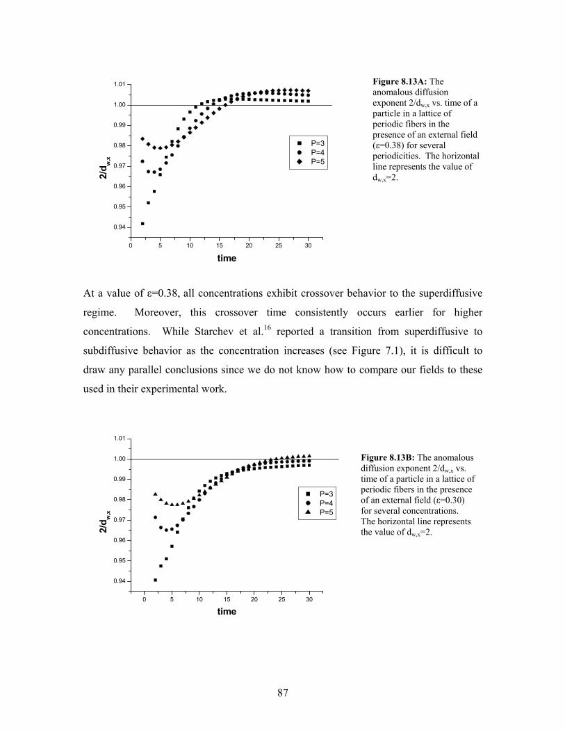
87
0 5 10 15 20 25 30
0.94
0.95
0.96
0.97
0.98
0.99
1.00
1.01
2/d w
,x
time
P=3 P=4 P=5
At a value of ε=0.38, all concentrations exhibit crossover behavior to the superdiffusive
regime. Moreover, this crossover time consistently occurs earlier for higher
concentrations. While Starchev et al.16 reported a transition from superdiffusive to
subdiffusive behavior as the concentration increases (see Figure 7.1), it is difficult to
draw any parallel conclusions since we do not know how to compare our fields to these
used in their experimental work.
0 5 10 15 20 25 30
0.94
0.95
0.96
0.97
0.98
0.99
1.00
1.01
2/d w
,x
time
P=3 P=4 P=5
Figure 8.13A: The anomalous diffusion exponent 2/dw,x vs. time of a particle in a lattice of periodic fibers in the presence of an external field (ε=0.38) for several periodicities. The horizontal line represents the value of dw,x=2.
Figure 8.13B: The anomalous diffusion exponent 2/dw,x vs. time of a particle in a lattice of periodic fibers in the presence of an external field (ε=0.30) for several concentrations. The horizontal line represents the value of dw,x=2.

88
In Figure 8.13B, we show data for a slightly lower field intensity ε=0.30. For higher
concentrations, the long-term behavior of the anomalous diffusion exponent is
subdiffusive for all times. As the concentration decreases however, we now clearly see a
transition from the subdiffusive regime to the superdiffusive regime. Therefore, choosing
an appropriate value of the electric field, we succeeded in reproducing (qualitatively) the
results of ref [16]. This is an important finding because it allows us to theoretically
reproduce experimental results thus validating both the results of ref [16] in addition to
our own model.
In section 8.2.1, we explored the dynamics of a particle in a lattice of periodic
obstacles in the presence of an external field. We presented the trivial results showing
that the mean motion in directions perpendicular to the external field is zero. We also
showed that the mean square displacement of the particle in the direction of the external
field is consistent with eq. (7.6), showing a transition from the diffusion towards the drift
regime. Nevertheless, the study of drift was not strictly the purview of the work so we
can simply resign ourselves to the statement that our results, so far, are consistent with
basic knowledge of diffusion dynamics, and, more to the point, consistent with the
experimental results of Starchev et al.16.
Staying faithful with the work of ref [16], we studied the second moment of
displacement (eq. 7.7) to effectively filter out the drift portion of the displacement in the
direction of the external field and study the diffusive properties of our particle. In doing
so, we studied the anomalous diffusion exponent, dw,x, by changing 2 parameters: the
obstacle concentration and the value of the external field.
By varying the external field, we discovered that the anomalous exponent made the
transition from subdiffusion to superdiffusion as the external field increases (Figure
8.12). Since Starchev et al.16 did not change their value of the external field we have no
basis for comparison. Nevertheless, we do observe for the first time that the electric field
does have an effect on the scaling exponent of the diffusion constant instead of simply
contributing to the particle’s drift. Therefore, when studying the short time displacement
of particles, we have to take this factor into consideration to obtain exact results. By
changing the lattice concentration, we successfully reproduced the results of Starchev et

89
al.16: Using an appropriate value of the external field (Figure 8.13B) we observed a
transition from subdiffusion to superdiffusion as the concentration was decreased.
The overall results reported so far in this section can be viewed as qualitatively
consistent with those found in ref [16]. The quantitative differences between our results
and those of Starchev et al.16 can be explained as follows: Firstly, the lattice used does
not adequately simulate the agarose gel used experimentally. The lattice of periodic
fibers used in this work is significantly different than an agarose gel and so we do not
make any claim to their similarity. Despite this important difference in gel architecture,
we reproduced similar qualitative results. The only remaining difference between our
theoretical results and those of ref [16] is the amplitude of the anomalous diffusion
exponent, dw, (Starchev et al.16 reported values of dw ranging from approximately
dw=1.42 – 3.64) presumably caused by the fractacality of the agarose gel. Secondly, the
disparity in the time and length scales may not allow us to compare results quantitatively.
We can then speculate that the strong anomalous diffusion observed experimentally
might be due either to the disorder of the distribution of obstacles or the trapping that
occurs within the gel due to its fractal nature, or both. To distinguish the importance in
these two factors, we propose a second gel, designed to isolate the trapping effect in
particle displacement while maintaining the idea of periodicity. Our goal is to confirm
whether trapping alone can reproduce results observed experimentally using an agarose
gel. The proposed lattice is shown in Figure 8.14 and the following section presents our
results using this new lattice.

90
8.2.2. A system with periodic traps
In Figure 8.14 we see 2 views of the proposed system. As can be seen, the purpose is
to impede the particle’s movement in the x-direction by introducing a periodic, funnel
shaped and hollow obstacle. In Figure 8.15A, we see the fractal dimension, dw,x, of the
diffusive motion of the particle as a function of time for several values of the external
field. The data shown for the particle without external field is qualitatively similar to
what was obtained in the lattice of periodic fibers. The important distinction, however, is
that convergence to the steady-state values appears to be much slower. Comparing with
Figure 8.5A, we can see that the amplitude of dw,x is indeed greater than what was
observed for the lattice of periodic obstacles and that the anomalous diffusion does
persist for much longer times. In fact, a long intermediate regime exists where
1.12 , >xwd if the field exceeds about ε=0.2. This is a new effect. In Figure 8.15B, we
see the transverse fractal dimension, dw,y. The data shown indicates that for all field
strengths, we have subdiffusive behavior. Ironically, in an attempt to trap a particle’s
movement in the x-direction, we also succeeded in achieving trapping dynamics in the y
and z-directions. For ε≤ 0.2, we can see how dw,y begins the slow transition to dw,y=2 at
Y
X X=7
X=6 X=2,3,4,5
X=0 X=1
Z
Y
Figure 8.14: A cross-section view of the dead-end matrix. On the left side we see the x-y plane. From this view we can see how the obstacles are arranged like a funnel, effectively trapping the molecules in the x-direction. On the right we see the Y-Z plane. The size of the whole cell is 8x8x8=512 lattice sites.

91
the steady-state. Longer times would have to be studied to observe this effect for larger
values of ε.
0 5 10 15 20 25 30
0.95
1.00
1.05
1.10
1.15
1.20
1.25
2/d w
,x
time
ε=0 ε=0.1 ε=0.2 ε=0.4 ε=0.5
0 5 10 15 20 25 30
0.91
0.92
0.93
0.94
0.95
0.96
0.97
0.98
0.99
2/d w
,y
time
ε=0 ε=0.1 ε=0.2 ε=0.4 ε=0.5
In Figures 8.16 and 8.17, we show the mean displacement and the mean square
displacement of a particle with a value of ε=0.2.
Figure 8.15A: xwd ,2 vs. time, t in a lattice of periodic traps for various values of the external field. The horizontal line indicates the value 2/dw,x=1.
Figure 8.15B: ywd .2 vs. time, t in a lattice of periodic traps for various field strengths.

92
-0.2 0.0 0.2 0.4 0.6 0.8 1.0 1.2 1.4 1.6-0.8
-0.6
-0.4
-0.2
0.0
0.2
0.4
0.6
0.8
1.0
m=0.952(
2)
m=0.982
(2)
m=1.17
6(2)
m=0.977
(2)
log(
<X2 >)
, lo
g(<Y
2 >)
log(time)
log(<Y2>) log(<X2>)
Figure 8.16 depicts the same physical behavior as the particle in a lattice of periodic
fibers: the velocity in the direction of the field is constant while the orthogonal velocities
are zero. Results shown in Figure 8.17 for the mean square displacement are interesting.
As in Figure 8.9B, the value of the slopes, m, provide the scaling exponents at t=1-3 and
t=27-30 for the displacement in the x and y directions respectively. We see that, initially,
the scaling exponent for both directions is subdiffusive ( )12 <= wdm . However, the
scaling of the mean square displacement is greater in the y-direction than the x-direction.
As the time increases, the diffusion exponent resumes its expected behavior: in the x-
direction we have a transition to the drift regime caused by the presence of the electric
field. In the y-direction, not only does the scaling remain subdiffusive but it is lower than
its initial value. We observed a much more rapid progression of the value of the scaling
exponent to its characteristic steady-state value (2/dw=1|t→∞) in the lattice of periodic
0 5 10 15 20 25 30
0.0
0.2
0.4
0.6
0.8
1.0
1.2
1.4<x
>, <
y>
time
<X> <Y>
Figure 8.16: The mean displacement of a particle against time in a lattice of periodic funnel-shaped traps with an external field parallel to the x-axis (ε=0.2). The squares represent the movement along the x-axis while the circles show the movement along the y-axis
Figure 8.17: Log-log plot of the mean square displacement of a particle against time in a lattice of periodic funnel-shaped traps with an applied field parallel to the x-axis (ε=0.2). The squares represent the movement along the x-axis while the circles show the movement along the y-axis. The values, m of the slopes for the first and last 3 points of each curve are shown.

93
fibers (see Figure 8.9B). The funnel-shaped lattice depicts a much slower transition to
the expected long-term behavior, as can clearly be seen in both Figures 8.15 and 8.17.
Since the transition to the steady-state regime is so slow, we plotted (dw-2) vs. 1/t in
Figure 8.18 to try to estimate the likely long-term behavior of the displacement of the
particle.
0.0 0.1 0.2 0.3 0.4 0.5
-0.30
-0.25
-0.20
-0.15
-0.10
-0.05
0.00
0.05
0.10
d w,x-2
1/t
The conclusion to be drawn from Figure 8.18 is that much longer times will need to be
studied to determine the way the anomalous exponent converges towards its asymptotic
value 2.
When we studied the lattice of periodic fibers, we plotted the second moment of the
displacement against time and showed how there is a crossover behavior at time t~8
where the second moment in the x-direction overtakes the second moment in the y-
direction. Results for the second moment of a particle in our lattice of periodic traps are
shown in Figure 8.19.
Figure 8.18: (dw,x-2), vs. 1/t of a particle in a lattice of funnel -shaped traps for several values of the external field. The horizontal line represents the value dw=2. The legend is as follows:
Symbol ε 0 0.1 0.2 0.3 0.4

94
-0.2 0.0 0.2 0.4 0.6 0.8 1.0 1.2 1.4 1.6-0.8
-0.6
-0.4
-0.2
0.0
0.2
0.4
0.6
0.8
1.0
m=1.085(1)
m=0.9397(8)
m=0.980(3)m=0.966(2)
log(
X-<X
>)2 , l
og(Y
-<Y>
)2 ))
log(time)
Y X
In the funnel-shaped lattice, the second moment in the x-direction is always greater than
the second moment in the y-direction (ie: ( ) ( ) tyyxx ,22 ∀−>− ). In terms of
their scaling exponent (which is indicated by the slope, m, of Figure 8.19), it is initially
lower in the x-direction and gradually increases in value until it is slightly higher than the
diffusion scaling in the y-direction. Consequently, short-time trapping the molecule in
the direction of the field is observed. As time increases, we see a transition to the super-
diffusive regime in the x-direction while we have sub-diffusion in the y-direction.
8.3 Discussion In this section, we will go over all results obtained in the second part of the thesis to
gain a better appreciation of this new model’s strong and weak points. After the
presentation of the model (Section 7.3), we showed that, in the absence of obstacles, there
is no transient regime and that the diffusion constant is not a function of time (Figure
8.1). Adding the presence of obstacles will cause the displacement of the particle to
undergo a sub-diffusive regime for short times when no external field is present. We call
this regime: ‘anomalous diffusion’. The extent and duration of the anomalous diffusion
regime is a function of the obstacle concentration and their distribution. One of our goals
was to determine how the transition from anomalous to steady-state diffusion is achieved.
Figure 8.19: log-log plot of the second moment of the displacement against time of a particle in a lattice of periodic, funnel-shaped obstacles in the presence of an external field (ε=0.3). Circles and squares represent the displacement in the x and y direction, respectively.

95
In all cases studied, we found that this transition was a smooth function and not strictly
delimited by two distinct regimes of displacement. In fact, we determined that the
progression of the scaling of the diffusion coefficient towards its steady-state value
became a linear function of t1 (Figure 8.8) in a lattice of periodic infinite fibers.
Moreover, we were able to find the mathematical relationship depicting the time, tmax, at
which the maximum value of dw was found (eq. 8.5) for a lattice of periodic infinite
fibers.
The time at which the maximum value of dw,x was achieved and a linear progression
towards the value dw,x=2 was subsequently observed was dependent on the periodicity, or
pore size, in our lattice of periodic infinite fibers. In contrast, no such linear relationship
was found for the lattice of periodic obstacles. Consequently, the relationship between
the gel architecture and the manner in which a particle makes the transition to steady-
state diffusion dynamics is not always easy to determine.
In the absence of an external field, the obstacle distributions that we studied did not
play a large role in the magnitude of dw,x. The maximum value of the fractal dimension
found using infinite periodic obstacles (dw,x=2.131, P=3, Figure 8.12 ) was about the
same as that which was found in a lattice of periodic traps (dw,x=2.132, Figure 8.15A).
Despite similar results with regards to the magnitude of the fractal dimension, the time
spent in an anomalous regime appears to be quite sensitive to the gel architecture. For
example, by comparing Figures 8.12 and 8.15A, we see how the particle spends a much
longer time in a subdiffusive regime in the lattice of periodic traps (dw,x~2.10|t=30) than
the lattice of periodic infinite fibers (dw,x~2.04|t=30). Indeed, the convergence of the
fractal dimension to the steady-state value is much slower in the lattice of periodic traps.
In all gels studied (periodic obstacles, infinite fibers and periodic traps), the value of
the fractal dimension was always close to 2 ( 193.02 −≅wd ) when no external field was
applied. Starchev et al.16 reported values of wd2 ranging from approximately 0.50-0.85
(see our Figure 7.1). Since our lattices do not simulate an agarose gel we can reasonably
state that the fractacality and/or disorder of the gel can also play an important role in the
amplitude of the anomalous diffusion effect.

96
When we consider the movement of the particle under the effect of an external field,
we showed that the initial (t=1-2) scaling exponent, xwd ,2 of the diffusion constant is a
decreasing function of the obstacle concentration (Figure 8.11). We also observed that
in a lattice of periodic obstacles, the particle can exhibit superdiffusive behavior when the
external field is sufficiently high (Figure 8.13A, 8.13B). Starchev et al.16 reported similar
findings. However, for small values of the external field we did not observe any
superdiffusive behavior ( )0.2 , 2, ≤∀> εtd xw . At higher values of the external field, we
initially (i.e. short times) have a subdiffusive regime (dw,x>2) followed by a
superdiffusive regime (dw,x<2). The exact value of the external field at which such a
transition is observed will depend on the obstacle concentration but is typically found to
be in the range 4.02.0 −=ε for the concentrations studied in this work. We predict that
the transition from sub to super-diffusion can be expressed as a function of time. This
new effect was never previously observed either experimentally, or numerically. Since
ref [16] only examined a single value of the external field, they were not able to
recognize how the magnitude of the external field can be significant when studying the
anomalous diffusion of particles. Moreover, the value of dw,x for a particle in a lattice of
periodic fibers was still much smaller than those reported by ref [16] when an external
field was applied. Although superdiffusion was observed, the observed range was
typically: 2.120.1 , << xwd . Starchev et al.16 observed values the were slightly larger
(up to 3.12 , ≅xwd (see our Figure 7.1)).
When we applied an external field to our funnel lattice, the transition to the steady-
state diffusion regime was very slow. If the external field was sufficiently low (ε<0.2),
we observe subdiffusion in all directions. For larger values of the external field (ε>0.2),
we observe a transition from the subdiffusive to the superdiffusive regime in the direction
of the external field (x) and very strong subdiffusive behavior in the other 2 directions
(y,z). The transverse fractal dimension was typically in the range: 0.129.0 , << ywd .
Ref [16] reports values of the transverse fractal dimension to be in the same range as
those found in the absence of an applied external field (i.e.: 0.55-0.85). However, we see
in Figure 8.15B that for larger values of the external field (ε>0.3), the maximum value of
dw,yz has not yet been reached and the transition towards the steady state value was not

97
observed. Therefore, our reported values of the fractal dimensions are somewhat
understated because the study of longer times would obviously indicate larger values of
the fractal dimension. When the external field is sufficiently high our lattice of periodic
funnels acts as an effective trap. Larger times will need to be studied to obtain more
consistent quantitative results.
In summary, we conclude that trapping does indeed play an important role in the
magnitude of dw. Since our reported values of the fractal dimension of the particle were
not as high as those found by Starchev et al.16 (or in the literature for that matter37,47,48)
we can only conclude that while trapping plays an important role in the particle’s short-
time subdiffusive behavior, the disorder and the fractacality of the gel also need to be
considered. A likely next step would be to study the short-time diffusion of particles in
disordered and fractal gels. Regular fractals, with periodic boundary conditions, would
be particularly useful.
The model proposed in the second part to this thesis does have inherent
disadvantages. Firstly, while any enumeration method has the advantage of providing
exact results, we do have to contend with the fact that we were only able to simulate very
short times. Exceeding t~50 becomes extremely time-consuming in three dimensions.
The study of t>50 is better left using stochastic algorithms. Secondly, it is not always
possible to extrapolate steady-state values for the displacement of particles. Although we
were able to find some exact values of the long term diffusion coefficient, we do not yet
have an expression linking the time at which progression towards the steady state value
becomes a linear function of t1 , allowing us to reliably extrapolate our results
to ∞→t
5 416
8415
8415
414h :fieldWith
5 416
415
415
414 :fieldWithout
=
+
−+
++
=
=
+
+
+
=
εε
h
∑= ik CF →∞→ M|1υ M1
01 →t . Moreover, our model will never be able to bridge the gap between anomalous
and steady-state behavior because we are limited to t<50. The studied particle would
have to traverse a distance that is several times greater than its average pore size before
achieving steady-state motion. In our model, being limited to t<50, the average distance

98
traversed by our particle is always of the order of a single pore size, even when the
external field is relatively high. Therefore, the use of exact enumeration models will
have to rely on extrapolation to determine the long term behavior of a particle.

99
PART III
Chapter 9
Conclusion
In this part of the thesis, we conclude by providing a discussion on the broad strokes
of what we accomplished. In each part of the thesis, we introduced a model that studied
various aspects of polymers physics. For each of these parts, we will present a short
synopsis of the model followed by a brief review of our major findings.
In the first part of the thesis we improved upon an existing model which found exact
values of the mobility of particles. We restructured the model to include the study of
small macromolecules. This improvement allowed us to study various new problems
because the molecular architecture is taken into consideration. Since the model was
independent of the molecular lattice description we opted to use the bond fluctuation
model to maximize the precision of our results at the expense of being limited to very
small molecular sizes.
The strong points of this new model is that you can obtain highly precise results for
the mobility (or diffusion coefficient) of a molecule without having to resort to lengthy
stochastic simulation algorithms. Moreover, our method provides complete flexibility
with regard to lattice descriptions, allowing for different rule sets for both molecule-
molecule and molecule-obstacle interactions. In other words, we can alter the lattice
description to suite our needs for the study of molecules in either 2 or 3 dimensions.
To accentuate the usefulness of this model, we will briefly reiterate some of our key
results. Firstly, we were able to clearly show the existence of entropic trapping.
Previous studies only speculated that entropic trapping may be exploited in sieving

100
matrices. In our study, we clearly showed how a molecule can be trapped between 2
walls and that the extent of the trapping will be a function of the molecular size.
Unfortunately, we were not able to study a large enough sample of molecular sizes to
determine how effectively we can sieve molecules using this technique. Secondly, we
used standard Ogston tools25 to determine that the effective gel radius is, in fact, a
function of molecular architecture. This means that the gel fibers will be able to affect
the mobility of the molecule, even when the two are far apart and that we must now
consider the gel along with the molecule to determine how the gel will affect the
mobility of the analyte. These were only two of many dynamic effects that we were
able to investigate using this model.
The model introduced in the first part of the thesis investigated systems in two-
dimensions, using only the bond fluctuation model to describe how the particles interact
with one another. A likely next step would be to study various lattice descriptions in
two-dimensions and compare our results to ascertain the importance of how we describe
our molecular interactions. Since our model can easily accommodate three-dimensional
systems, we can also study analytes in 3D. This would be the next step, especially if we
wish to use this model to aid in the development of experimental sieving systems.
In the second part of the thesis, we focused on the short-time anomalous diffusion of
particles. We proposed an exact enumeration model designed to study the short-time
displacement of point-like molecules. We enumerated all possible particle trajectories
and associated probabilities to each trajectory to determine the exact displacement of the
particle. Quantities that were studied included the time-dependent diffusion constant
D(t) and the fractal dimension, dw, whose value translates directly to the scaling of the
particle’s displacement. We studied these system parameters by varying the obstacle
distribution, concentration (C) and applied (dimensionless) external field (ε) to
determine how these factors affect the manner in which a particle achieved its
characteristic steady-state displacement.
To validate the model, we studied a particle in both solution (ie: C=0, no obstacles)
and by using simple obstruction schemes (ie: periodic obstacles and periodic infinite
fibres). Our results corresponded very well to both theoretical predictions and
comparison with published results. During our validation process, we identified that, in

101
some cases, the long-term steady-state solution to the diffusion constant, Do, can be
extrapololated linearly to 01 →t . Additionally, we were also able to duplicate
(qualitatively) all the results reported by Starchev et al.16. Specifically, we observed
transition from subdiffusive to superdiffusive behavior of the particle in the presence of
an applied external field as the concentration decreases (Figure 8.13B).
We also studied a potential trapping lattice (shown in Figure 8.14) to determine the
extent to which the anomalous diffusion effect is caused by trapping within a gel (as
opposed to gel disorder). We determined that this trapping lattice displayed anomalous
diffusion for much greater times than in a lattice without trapping. In other words, the
transition to the steady state regime was decidedly much slower. We also showed that
for higher values of the external field, the particle in the funnel shaped lattice displayed
significant superdiffusion in the direction of the field while in the y,z directions, we
observed significant subdiffusion. The general theme identified with this lattice was that
much longer times would need to be studied to fully characterize the extent of the
anomalous diffusion for both magnitude and time scales.
In this second part, we showed that the physics involved in the short-time
displacement of particles are indeed significant and deserve to be studied in more detail
to gain a better understanding of the short-time displacement of particles. We only
began this study by showing a few interesting lattice models that were designed to show
the validity and scope of this new model. A more detailed investigation using disordered
gels seems in order. A model that can study longer times would also prove quite useful
to help bridge the gap in our understanding between the short time and steady-state
regimes of displacement.

102
References
1. Stellwagen, N., Gelfi, C., Righetti, P.G., Electrophoresis, 2002, 23, 167-175
2. Krylov, S.N., Dovichi, N.J., Analytical Chemistry, Vol. 72, No. 12, June 15, 2000
3. Marquet, C., Buguin, A., Talini, L., Silberzan, P., Physical Review Letters , Vol
88, No. 16, 22 April 2002
4. Huang, L.R., Tegenfieldt, J.O., Kraeft, J.J., Sturm, J.C., Austin, R.H., Cox, E.C.,
Nature Biotechnology, 2002, 20, 1048-1050
5. Morris, C.J.O.R., in: Peeters, H. (Eds.), Protides of the Biological Fluids,
Elsevier, New York 1967, pp. 543-551.
6. Rodbard, D., and Chrambach, A., Proc. Nat Acad. Sci. USA 1970, 65, 970-977.
7. Tietz, D., in: Chrambach, A., Dunn, M. J., Radola, B. J. (Eds.) Advances in
Electrophoresis Volume 2, VCH Publishers, Weinheim 1988, pp. 109-169
8. Mercier, J,-F., Slater, G. W., J. Chem. Phys. 1999, 110, 6050-6056.
9. Mercier, J,-F., Slater, G. W., J. Chem. Phys. 1999, 110, 6057-6065
10. Slater, G. W., Guo, H. L., Electrophoresis. 1996, 17, 977-988.
11. Slater, G. W., Guo, H. L., Electrophoresis. 1996, 17, 1407-1415.
12. Treurniet, J. R., Slater, G. W., J. Chromatography A 1997, 772, 39-48.
13. Mercier, J.-F., Slater G. W., Electrophoresis 1998, 19, 1560-1565.
14. Doi M., Edwards S. F., The theory of Polymer Dynamics, Clarendon Press,
Oxford 1986
15. R.K. Pathria, Statistical Mechanics 2nd ed. (Butterworth Heinemann, Oxford,
(1996)
16. Starchev, K., Sturm, J., Weill, G., Brogren, C.-H., Journal of Physical Chemistry
B, 1997, 101, 5659-5663
17. Ogston, A.G., Trans. Faraday Soc. 1958, 54, 1754-1757.
18. Ferguson, K. A., Metabolism 1964, 13, 985-1002.
19. Slater, G. W., Guo, H. L., Electrophoresis 1995, 16, 11-15
20. Mercier, J. F., Slater, G. W., Electrophoresis 1998, 18, 1560-1565

103
21. Labrie, J., Mercier, J.-F., Slater, G. W, Electrophoresis 2000, 21, 823-833.
22. Reif, F., Fundamentals of statistical and thermal physics, McGraw-Hill, 1965.
23. G. W. Slater, J. Rousseau and J. Noolandi, Biopolymers 26, 863 (1987).
24. D. W. Heermann, Computer simulation methods, 2nd ed. (Springer-Verlag. 1990)
25. Slater, G.W., “Theory of band broadening for DNA gel electrophoresis and
sequencing” Electrophoresis 14, 1-7 (1993)
26. Carmesin I., Kremer K., Macromolecules 1988, 21, 2819-2823
27. Press, W. H., Flannery, B. P., Teukolsky, S. A., Vetterling, W. T., Numerical
Recipes: The Art of Scientific Computing (fortran version), Cambridge University
Press, Cambridge (1989)
28. Bishop, M., Michels, J. P. J., J. Chem. Phys. 1985, 83, pp. 4791-4792.
29. Nixon, G. I., Slater, G. W., Phys. Rev. E 1999, 60, pp. 3170-3173.
30. Slater, G. W., Nixon, G. I., Physics in Canada 1997, 53, pp. 177-183
31. Rousseau, J., Drouin, G., Slater, G. W., Phys. Rev. Lett. 1997, 79, pp. 1945-1948
32. A. Meller, D Branton, Electrophoresis 2002, 23 pp. 2583-2591
33. Cabodi, M., Turner, S. W. P., Craighead, H., G., Analytical Chemistry, Vol. 74,
No. 20, October 15, 2002
34. Heukelum, A. V., Barkema, G. T., Bisseling, R. H., Journal of Computational
Physics 180, pp. 213-326 (2002)
35. Stauffer, D., Introduction to Percolation Theory: Taylor & Francis: London,
1985: p. 95
36. Havlin, S. Molecular Diffusion and Reactions, In The fractal Approach to
Heterogenous Chemistry; Avnir, D., Ed.; John Wiley & Sons: New York, 1989
37. Havlin, S.; Ben-Avraham, D. Adv. Phy. 1987, 36, pp. 695-798
38. De Gennes, P. G., J. Chem. Phys., 22, 1971, pp. 572-579
39. Saxton, M. J. Biophys. J. 1992, 61, 119-128
40. Saxton, M. J. Biophys. J. 1993, 64, 1053-1062
41. Mandelbrot, The Fractal Geometry of Nature; W.H. Freeman and Co.: New York,
1982.
42. Slater, G. W.; Guo, H. L. Electrophoresis 1995, 16, 11-15.
43. Starchev, K.; Avramov, M.; Radoev, B. Langmuir 1995, 11, 1731-1734.

104
44. Gauthier, M. G., Slater, G. W., J. Chem. Phys., 117, 2002, pp. 6745-6756
45. Slater, G.W.; Wu, Y.S., Phys. Rev. Lett., 1995, 75, 164-167
46. Majid, I., Ben-Avraham, D., Havlin, S., Stanley, H. E., Phys, Review B, 1984, 30,
1626-1628
47. Rampino, N. J, Chrambach, A. J., Chromatogr. 1992, 596, 141-149
48. Havlin, S., Molecular Diffusion and Reactions. In The Fractal Approach to
Heterogeneous Chemistry; Avnir, D., Ed.; John Wiley & Sons: New York, 1989
49. B. Maier and J. O. Radler, Phys Rev. Lett., 1999, 82, 1911
50. P. Cicuta and I. Hopkinson, J. Chem Phys., 114, 2001, pp. 8659
51. Grant I. Nixon, Gary W. Slater, J. Chem. Phys., 117, 2002
52. Mercier, J-F., Slater, G.,W., Macromolecules 2001, 34, 3437-3445