investigation of a multilevel inverter for electric
TRANSCRIPT

Investigation of a Multilevel Inverterfor Electric Vehicle Applications
Oskar Josefsson
Department of Energy and EnvironmentCHALMERS UNIVERSITY OF TECHNOLOGY
Göteborg, Sweden 2015


THESIS FOR THE DEGREE OF DOCTOR OF PHILOSOPHY
Investigation of a Multilevel Inverterfor Electric Vehicle Applications
Oskar Josefsson
Division of Electric Power EngineeringDepartment of Energy and Environment
CHALMERS UNIVERSITY OF TECHNOLOGYGöteborg, Sweden 2015
Investigation of a Multilevel Inverter
for Electric Vehicle Applications
Oskar JosefssonISBN 978-91-7597-174-2
c© Oskar Josefsson, 2015.except where otherwise stated.All rights reserved
Doktorsavhandlingar vid Chalmers tekniska högskolaNy serie nr 3855ISSN 0346-718X
Department of Energy and EnvironmentCHALMERS UNIVERSITY OF TECHNOLOGYSE-412 96 GöteborgSwedenTelephone + 46 (0)31 772 10 00
Printed by Chalmers Reproservice,Gothenburg, Sweden, 2015

To my family
iii

iv

Abstract
Electrified vehicles on the market today all use the classical two-level in-verter as the propulsion inverter. This thesis analyse the potential of usinga cascaded H-bridge multilevel inverter as the propulsion inverter. With amultilevel inverter, the battery is divided into several parts and the invertercan now create voltages in smaller voltage levels than the two-level inverter.This, among other benefits, reduces the EMI spectrum in the phase cablesto the electric machine. It is also shown that these H-bridges can be placedinto the battery casing with a marginal size increase, and some addition ofthe cooling circuit performance. The benefit is that the separate inverter canbe omitted.
In this thesis, measurements and parameterisations of the battery cellsare performed at the current and frequency levels that are present in a mul-tilevel inverter drive system. The derived model shows a great match to themeasurements for different operating points and frequencies.
Further, full drive cycle simulations are performed for the two analysedsystems. It is shown that the inverter loss is greatly reduced with the multi-level inverter topology, mainly due to the possibility to use MOSFETs insteadof IGBTs. However, the battery packs in a multilevel inverter experience acurrent far from DC when creating the AC-voltages to the electric machine.This leads to an increase of the battery loss but looking at the total inverter-battery losses, the system shows an efficiency improvement over the classicaltwo-level system for all but one drive cycle. In the NEDC drive cycle thelosses are reduced by 30 % but in the demanding US06 drive cycle the lossesare increased by 11 % due to the high reactive power demand at high speeddriving. These figures are valid for a plug-in hybrid with a 50 km electricalrange where no filter capacitors are used. In a pure electric vehicle, there isalways an energy benefit of using a multilevel converter since a larger batterywill have lower losses. By placing capacitors over the inputs of the H-bridges,the battery current is filtered. Two different capacitor chemistries are anal-ysed and experimentally verified and an improvement is shown, even for asmall amount of capacitors and especially at cold operating conditions.
v

Keywords
Electric Vehicle (EV), Plug-in Electric Vehicle (PEV), Multilevel Inverter(MLI), Two-level Inverter (TLI), Integrated Charger, Drive Cycle, Efficiency,Battery modelling, LiFePO4.
vi
Acknowledgement
The financial support from the Swedish Energy Agency and Volvo Car Cor-poration is gratefully appreciated.
I would like to direct a very special thank you to my examiner and mainsupervisor Torbjörn Thiringer, the support and discussions are truly appre-ciated. Thank you for taking the time! I would also like to thank SonjaLundmark as co-supervisor and Anders Lindskog for the introduction of theproject.
A big thank you to all the colleges at the division of Electric Power En-gineering, the atmosphere among the colleagues is excellent and it has beena privilege to work here and to just sit down and have a chat in the lunchroom. A sincere thank you to my very special friends and office colleaguesDavid Steen and Elias Hartvigsson for making it a pure joy coming to work.
At last I want to thank my family and friends. It is you who add valueto my life, thank you for being part of it!
Oskar JosefssonGöteborg, February 2015
vii

viii
Contents
Abstract v
Acknowledgement vii
List of Nomenclatures xiii
1 Introduction 1
1.1 Background . . . . . . . . . . . . . . . . . . . . . . . . . . . . 1
1.2 Purpose of work . . . . . . . . . . . . . . . . . . . . . . . . . 4
1.3 Contributions . . . . . . . . . . . . . . . . . . . . . . . . . . . 4
2 Drive system topologies and control 7
2.1 Two-level inverter . . . . . . . . . . . . . . . . . . . . . . . . . 7
2.1.1 PWM . . . . . . . . . . . . . . . . . . . . . . . . . . . 7
2.1.2 Third harmonic injection(THI)-PWM . . . . . . . . . 8
2.2 Cascaded full-bridge multilevel inverter . . . . . . . . . . . . 10
2.2.1 Fundamental Selective Harmonic Elimination (FSHE) 11
2.2.2 Balancing strategy for MLI . . . . . . . . . . . . . . . 16
2.3 Electric machine and torque control . . . . . . . . . . . . . . 16
2.4 Charger . . . . . . . . . . . . . . . . . . . . . . . . . . . . . . 17
3 Inverter loss modeling 21
3.1 Power electronic components . . . . . . . . . . . . . . . . . . 21
3.1.1 MOSFET losses . . . . . . . . . . . . . . . . . . . . . 22
3.1.2 IGBT losses . . . . . . . . . . . . . . . . . . . . . . . . 23
3.1.3 Diode losses . . . . . . . . . . . . . . . . . . . . . . . . 25
ix

3.1.4 Miscellaneous power electronic components . . . . . . 26
3.2 Two level inverter (TLI) . . . . . . . . . . . . . . . . . . . . . 26
3.2.1 Conduction losses . . . . . . . . . . . . . . . . . . . . 27
3.2.2 Switching losses . . . . . . . . . . . . . . . . . . . . . . 28
3.2.3 Total losses . . . . . . . . . . . . . . . . . . . . . . . . 29
3.3 Multilevel inverter (MLI) . . . . . . . . . . . . . . . . . . . . 29
3.3.1 Conduction losses . . . . . . . . . . . . . . . . . . . . 29
3.3.2 Switching losses . . . . . . . . . . . . . . . . . . . . . . 30
3.3.3 Total losses . . . . . . . . . . . . . . . . . . . . . . . . 31
4 Case setup & inverter waveform verification 33
4.1 Small PEV reference vehicle . . . . . . . . . . . . . . . . . . . 33
4.1.1 Electric machine . . . . . . . . . . . . . . . . . . . . . 34
4.1.2 Test vehicle battery . . . . . . . . . . . . . . . . . . . 35
4.1.3 Filter capacitors for the MLI system . . . . . . . . . . 37
4.1.4 Test vehicle power electronic components . . . . . . . 38
4.1.5 Drive cycle presentation . . . . . . . . . . . . . . . . . 39
4.2 Experimental system . . . . . . . . . . . . . . . . . . . . . . . 39
4.3 Experimental base verification . . . . . . . . . . . . . . . . . . 41
4.3.1 Output waveforms and harmonics . . . . . . . . . . . 41
4.3.2 Total Harmonic Distortion . . . . . . . . . . . . . . . . 45
4.3.3 Balancing using the experimental setup . . . . . . . . 46
4.3.4 Battery current verification with the experimental setup 48
5 Small PEV power train loss evaluation 51
5.1 Efficiency calculations . . . . . . . . . . . . . . . . . . . . . . 51
5.1.1 Inverter . . . . . . . . . . . . . . . . . . . . . . . . . . 51
5.1.2 Battery . . . . . . . . . . . . . . . . . . . . . . . . . . 56
5.1.3 Combined inverter and battery losses . . . . . . . . . . 59
5.1.4 Loss comparison . . . . . . . . . . . . . . . . . . . . . 61
5.1.5 Charging . . . . . . . . . . . . . . . . . . . . . . . . . 65
5.2 Drive cycle evaluation . . . . . . . . . . . . . . . . . . . . . . 66
5.2.1 NEDC . . . . . . . . . . . . . . . . . . . . . . . . . . . 66
5.2.2 FTP75 . . . . . . . . . . . . . . . . . . . . . . . . . . . 68
5.2.3 HWFET . . . . . . . . . . . . . . . . . . . . . . . . . . 69
x

5.2.4 US06 . . . . . . . . . . . . . . . . . . . . . . . . . . . . 70
5.2.5 Comparison between proposed topology and classicalinverter . . . . . . . . . . . . . . . . . . . . . . . . . . 71
5.3 40 kWh battery . . . . . . . . . . . . . . . . . . . . . . . . . . 72
5.4 Slim sizing of the inverter semiconductors . . . . . . . . . . . 74
6 Battery loss modeling 77
6.1 Parameter extraction . . . . . . . . . . . . . . . . . . . . . . . 78
6.2 Verification in experimental system . . . . . . . . . . . . . . . 79
6.2.1 Representative operating points for the full scale system 83
6.2.2 Battery model performance in the MLI . . . . . . . . 84
6.3 Drive cycle evaluation for battery losses . . . . . . . . . . . . 86
7 Filter capacitor influence 89
7.1 System overview . . . . . . . . . . . . . . . . . . . . . . . . . 89
7.1.1 Battery cell . . . . . . . . . . . . . . . . . . . . . . . . 89
7.2 Capacitor configurations . . . . . . . . . . . . . . . . . . . . . 92
7.3 Model verification . . . . . . . . . . . . . . . . . . . . . . . . 94
7.4 Frequency analysis . . . . . . . . . . . . . . . . . . . . . . . . 95
7.5 Drive cycle analysis . . . . . . . . . . . . . . . . . . . . . . . . 98
7.6 Cold climate performance . . . . . . . . . . . . . . . . . . . . 102
8 Proposal for packaging of the inverter-battery unit and its
cooling circuit 107
8.1 Two-level inverter . . . . . . . . . . . . . . . . . . . . . . . . . 109
8.2 MOSFET equipped cell voltage monitor modules . . . . . . . 110
8.2.1 Thermal resistance of the MOSFETs . . . . . . . . . . 113
8.2.2 Thermal properties of the PCB . . . . . . . . . . . . . 113
8.2.3 Heat sink for CVMM . . . . . . . . . . . . . . . . . . 113
8.2.4 Cooling circuit temperature increase due to battery losses114
8.2.5 Resulting thermal analysis for the MOSFET-enhancedCVMM system . . . . . . . . . . . . . . . . . . . . . . 114
8.3 Slim sized inverters . . . . . . . . . . . . . . . . . . . . . . . . 115
9 Conclusions 117
10 Future Work 119
xi

References 121
xii

List of Nomenclatures
The following list presents nomenclatures that are used throughout this the-sis:
MLI Multilevel Inverter
TLI Two-level Inverter
THI Third Harmonic Injection
FSHE Fundamental Selective Harmonic Elimination
CVMM Cell Voltage Monitor Module
ESR Equivalent Series Resistance
VCE IGBT collector emitter voltage
IC IGBT collector current
VtIGBTIGBT fixed voltage drop
RonIGBTIGBT resistance
VDS MOSFET drain source voltage
ID MOSFET drain current
RonMOSFETMOSFET resistance
Ton Transistor turn on time
Toff Transistor turn off time
VDiode Diode anode cathode voltage
IDiode Diode anode current
VtDiodeDiode fixed voltage drop
xiii

RDiode Diode resistance
Qrr Diode reverse recovery charge
Krr Diode reverse recovery equivalent loss parameter
ERR Diode reverse recovery energy
Vdrr Diode voltage at reverse recovery
Eon Transistor turn on energy
Eoff Transistor turn off energy
C Capacitance of one MLI H-bridge input capacitor
n Number of H-bridges for one phase in the MLI
N Number of voltage levels one phase can produce
VDCMLInput voltage for each H-bridge in the MLI
VDCTLInput voltage for the TLI
UphaseRMSMAXMaximum phase voltage that can produced by theinverters
UphaseRMSMAXTHIMaximum phase voltage that can produced by theTLI when controlled with third harmonic injec-tion
h Harmonic number
UML(h) Harmonic value at harmonic h for the MLI
α1 Angle where the first H-bridge is turned on
α2 Angle where the second H-bridge is turned on
α3 Angle where the third H-bridge is turned on
Vout(t) Inverter reference output voltage
U Amplitude of inverter reference output voltage
ω Frequency of inverter reference output voltage
ϕ Phase difference of inverter output voltage andcurrent
a Magnitude of third harmonic component
xiv

I Amplitude of inverter output current
ffund Frequency of inverter reference output voltage
Tf Time period of inverter reference output voltage
fsw Switching frequency of the TLI
ma Modulation index
D(t) Duty cycle of the TLI
PcondIGBT1HConduction losses for the upper transistor in theTLI
PcondIGBT1LConduction losses for the lower transistor in theTLI
PcondDiode1HConduction losses for the upper diode in the TLI
PcondDiode1LConduction losses for the lower diode in the TLI
PconductionIGBTs1Average conduction losses for the transistors inone leg in the TLI
PconductionDiodes1Average conduction losses for the diodes in oneleg in the TLI
PswitchIGBT1HSwitching losses for the upper transistor in theTLI
PswitchIGBT1LSwitching losses for the lower transistor in theTLI
PrrDiode1HSwitching losses for the upper diode in the TLI
PrrDiode1LSwitching losses for the lower diode in the TLI
PswitchIGBTs1Average switching losses for the transistors in oneleg in the TLI
PrrDiodes1Average switching losses for the diodes in one legin the TLI
PLossTLIAverage total loss in the TLI
Vdrop Phase voltage drop in the MLI
PconductionMLIConduction losses for the MLI
Eonα1...6Turn on energy at switching instance 1 to 6
xv

Eoffα1...6Turn off energy at switching instance 1 to 6
Errα1...6Reverse recovery energy at switching instance 1to 6
PswitchMLIAverage switching losses in the MLI
PLossMLAverage total loss in MLI
usd Stator voltage in d-direction
usq Stator voltage in q-direction
isd Stator current in d-direction
isq Stator current in q-direction
ψm Magnetic flux density
p Pole pairs
Rs Stator resistance
Ld Inductance in d-direction
Lq Inductance in q-direction
UphaseRMSMachine phase voltage
IphaseRMSMachine phase current
∠ ~us Angle of machine voltage relative to machine po-sition
∠~is Angle of machine current relative to machine po-sition
∆TwaterTLIinverterTemperature rise in water due to the inverter lossesin the TLI case
∆TwaterTLIbatteryTemperature rise in water due to the battery lossesin the TLI case
∆TwaterMLIinverterTemperature rise in water due to the inverter lossesin the MLI case
∆TwaterMLIbatteryTemperature rise in water due to the battery lossesin the MLI case
∆TwaterMLItotalTemperature rise in water due to the combinedbattery and inverter losses in the MLI case
xvi

∆TJ−A Temperature difference between the junctions andambient air for the transistors
TjunctionTLIinverterTemperature of the junctions of the IGBTs in theTLI
PTLIinverter TLI inverter losses used for thermal calculations
PTLIbattery TLI battery losses used for thermal calculations
PMLIinverter MLI inverter losses used for thermal calculations
PH−bridge MLI inverter losses for each H-bridge used forthermal calculations
PMLIbattery MLI battery losses used for thermal calculations
∆V∆t Water flow in cooling circuit
Cp Specific heat capacity of the cooling fluid
ρ Density of the cooling fluid
RthJ−water Thermal resistance from the junctions of the tran-sistors to the cooling water
RthJ−C Thermal resistance from the junctions of the tran-sistors to the case
RthC−H Thermal resistance from the cases of the transis-tors to the heat sink
RthH−A Thermal resistance from the heat sink of the tran-sistors to ambient air
RthJ−A Combined thermal resistance from the junctionsof the transistors to ambient air
xvii

xviii

Chapter 1
Introduction
1.1 Background
Electrified vehicles (EVs) are occupying an increasing part of the market sharefor personal vehicles, both in the form of hybrid electric vehicles (HEVs) butalso pure battery electric vehicles (BEVs). Lately, most focus has been spenton the development of vehicles that can be charged from the network, pluginelectric vehicles(PEVs), with a driving distance of at least 20-30 km on pureelectricity. For the automotive manufacturer, one important challenge is todevelop a PEV with as long driving distance as possible for a given batterysize i.e. high drive train efficiency. A lot of development resources are spenton developing an aerodynamic vehicle which still attracts the customer interms of design and storage capabilities. Additionally, focus has to be spenton optimising the energy conversion from the chemical energy in the battery,through the power electronics as electrical power and finally to mechanicalenergy by the electrical machine.
To be able to optimise all the power conversions in the vehicle, goodunderstanding of the behaviour of the different components are needed. Itis also important to understand the operating points in terms of speed andtorque that the car is operated at, so that the components are optimisednot only at one operating point, but for the average of the whole operatingregion. A lot of research has been done in modeling the efficiency for elec-trified vehicles. Some simulation aspects are shown in [1] and [2], dealingwith both the physical modeling as well as the electrical one. It is shownthat even though it is important to analyse the efficiency of each compo-nent, the different components determine the operation points for each otherand therefore the complete drive train must be incorporated in the vehicleefficiency analysis since it is the combined total efficiency which is of interest.
1
The control strategy used for the power electronics highly affects the lossesin the vehicle as is shown by [3] and [4]. Also, depending on how the vehicleis used, some control strategies show a better performance. Having accuratemodels of the different components, but also how they affect each other de-pending on the control and operating point is of high importance in orderto achieve a good simulation result [5]. Since the car is operated in a widespeed range, simulations of full drive cycles are important to evaluate the ac-tual performance in the whole operating range and not only a few operatingpoints. It is of course also vital that the models are verified against mea-surements and/or empirical data, other models and analytical calculationswherever possible.
To be able to compare how good an electric vehicle drive train is, testprocedures are needed. Different test procedures for EVs are explained in [6]where it is stated that one problem for making accurate testing is to describeequivalent fuel consumptions for an electric vehicle since other vehicles aremeasured in liters of fossil fuel per kilometer. Today, PEVs are often countedas zero-emission vehicles but this might in the future change since a lot of theelectricity is still produced by fossil fuels, and then the energy efficiency inthe electrified vehicles will be of much more importance then today. In orderto compare different electric drive trains it is important to spend the focus tominimizing the drive train losses and thereby get the lowest fuel consumptionfor a given vehicle.
In order to evaluate different topologies of EVs, an analysis of the marketis needed [7]. It is stated by [8] and [9] that all EVs on the market today usethe same power electronic concept; the two-level inverter (TLI). However, itis indicated that an increase in research is expected for the power electronicsused for propulsion to develop competitive EVs [10]. The power electronicsplaced in an EV need to meet some special requirements and is discussed in[11] and [12]. Different power electronic packages, for example, give differentadvantages in terms of cooling which also affect the design of the coolingcircuits and packaging possibilities.
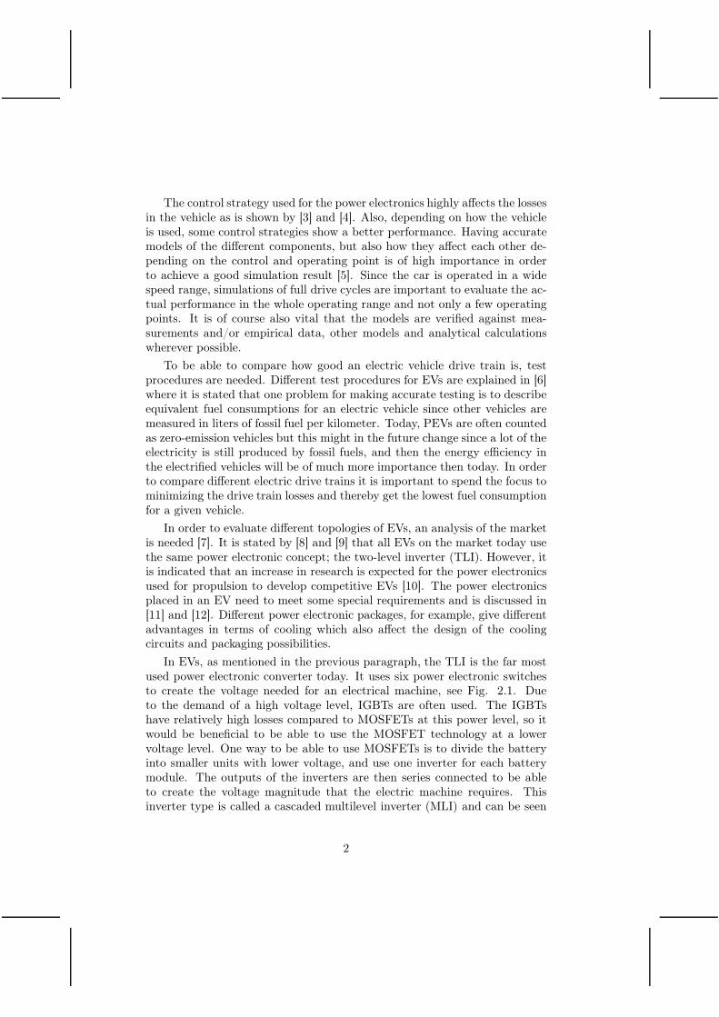
In EVs, as mentioned in the previous paragraph, the TLI is the far mostused power electronic converter today. It uses six power electronic switchesto create the voltage needed for an electrical machine, see Fig. 2.1. Dueto the demand of a high voltage level, IGBTs are often used. The IGBTshave relatively high losses compared to MOSFETs at this power level, so itwould be beneficial to be able to use the MOSFET technology at a lowervoltage level. One way to be able to use MOSFETs is to divide the batteryinto smaller units with lower voltage, and use one inverter for each batterymodule. The outputs of the inverters are then series connected to be ableto create the voltage magnitude that the electric machine requires. Thisinverter type is called a cascaded multilevel inverter (MLI) and can be seen
2
in Fig. 2.4. This converter topology is becoming popular for power systemapplications such as FACTS and HVDC [13]. How suitable this inverter typeis as propulsion inverter in electrified vehicles is however not evaluated so far.
Regarding battery representation, a battery can electrically be describedin many ways, see [14], [15], [16] and [17]. In simulations of electrified vehi-cles, the far most common way is to describe it as a purely resistive voltagesource with an open source voltage that is state of charge(SOC) dependant.However, the battery currents are far from DC [18] when using a MLI to pro-pel the vehicle and these models do not consider the frequency componentsthat the battery modules are subject to in a MLI drive system (1 Hz-10 kHz).Sometimes, in literature, the Randles model is used, [19], [20], [21] and [22],to account for the filtering effects the battery is subjected to during a drivecycle of the car which are in the range of seconds to minutes. A commonway to capture the high frequency behaviour of the battery is to use electro-chemical impedance spectroscopy. A problem with this method is that theparameters are subtracted at very low current levels, and might give differentresults than a substraction made at the operating point at which the batterywill be used in [23].
The PEV must have a charger to be able to charge the battery from thegrid. In the great majority of the electrical vehicles out on the market today,the charger is a stand-alone component. It can be either an on-board chargerthat is located in the vehicle, or it can be an off-board charger located atdifferent locations in the infrastructure. It is advantageous if the propulsionpower electronics can be used also for charging; then the separate powerelectronics in the on board charger is not needed, and space needs as well ascost can be reduced. This has been showed to work with the TLI, see [24],however, the consequences when doing the same with the MLI, is not yetevaluated for a vehicle application.
The advantages and benefits of using a MLI in an electrified vehicle arediscussed in [25] and in [26]. It is stated that the MLI has almost no elec-tromagnetic interference (EMI) and is therefore a safer and more accessiblechoice to have in a vehicle. One other benefit is for example if one batterycell in the battery pack has a lower capacity compared to the rest of the cells,the whole battery pack does not need to be used at the capacity level of thisweakest single cell. In a TLI this is the case but for the MLI only the cellswithin that battery group would need to be used less. The efficiency is alsodiscussed in general terms but without any quantification. The efficiency isonly predicted to be higher than the one for the TLI.
Obviously the MLI has advantages regarding EMI and battery utilisation,however, traceable results of the benefits of using a MLI in electrified vehiclesfrom an energy point of view, and to what extent, is missing.
3

1.2 Purpose of work
A possibility to improve the total electric drive train efficiency and thus toutilize the energy stored in the battery of the electrified vehicle, could be touse the MLI concept as an alternative to the commonly used TLI. However,this needs too be quantified using comparative calculations for these twoinverter topologies, using adequate model representations.
The purpose of this thesis is therefore to analyse the opportunities ofusing a MLI as the propulsion inverter in an electrified vehicle. The mainfocus is made on the energy efficiency when using different drive cycles andcontrol strategies in order to quantify the energy losses. Furthermore, sincethe MLI inverter loads the battery with a current far from DC, an adequateloss model must be parameterized, verified and implemented.
Finally, an important objective is to propose how the MLI could be prac-tically implemented and to make a crude thermal evaluation.
1.3 Contributions
According to the author the following contributions not found in previousavailable literature have been made with this thesis.
• Quantified the losses in an electric power train for the MLI in a completetorque-speed map, and put it in relation to the losses in a TLI. Thisanalysis is done, including the battery energy loss consequences, inorder to determine the difference between the systems for all relevantoperating points of the electric vehicle. Results also presented in [27]and [28].
• Performed an analysis of the electrical losses for the combined battery-inverter systems for different drive cycles in order to be able to quantifythe energy losses for the two systems. Results also presented in [28].
• Presented a proposal of implementation of the MLI system, removingthe discrete inverter, and performed a rough conservative thermal eval-uation of the suitability of such an implementation.
• Derived and quantified the importance of using an adequate batteryrepresentation for the MLI vehicle application, and verified these lossesexperimentally.
• Determined the energy loss consequences when using different typesof capacitors to alleviate the battery cells. This analysis is done boththeoretically and experimentally and the resulting EMI consequencesare also indicated.
4

• Experimentally verified the battery current waveforms from a MLI andexperimentally proved the possibility to balance the battery groupsduring driving.
5

6

Chapter 2
Drive system topologies and
control
To evaluate the performance and efficiency of a multilevel inverter (MLI) usedas the propulsion inverter, knowledge about the system is needed. To drawconclusions about the benefits, a reference system is also needed. Therefore,two different inverter topologies will be studied in this thesis. The cascadedmultilevel inverter (MLI) and the classical two-level inverter (TLI).
2.1 Two-level inverter
The TLI is by far the most common propulsion inverter used in electrifiedvehicles. It consists of six switches divided into three legs, see Fig. 2.1. Ananti-parallel diode is placed in anti-parallel to each switch to allow currentto flow in the reverse direction as well. The battery is connected to the inputof the inverter supplying it with a voltage level of VDCTL
. The inverter canproduce eight different states depending on the control of the six switches,where two are the zero voltage vector.
2.1.1 PWM
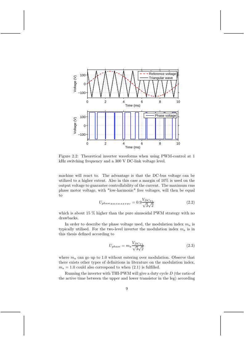
When a TLI is controlled in PWM-mode, three voltage references are createdas can be seen in Fig. 2.2. Observe that in Fig. 2.2 the switching frequencyis very low, only 1 kHz for illustrative purposes, for a PEV it is typicallyaround 10 kHz. These references are compared to a triangular wave with afrequency equal to the switching frequency. When the reference is higher thanthe triangular wave, the upper side switch in that leg is activated (turned
7

IGBT1H
IGBT1L
Diode1H
Diode1L
PMSM
+
VdcTL
-
Figure 2.1: Topology of a two-level inverter (TLI).
on), otherwise the lower side switch is activated. It is also possible to useover modulation, which means that the reference wave is above the peak ofthe triangular wave. This could be for one or several triangle wave periods.During the time the reference wave is above the peak of the triangular wave,no switching instances will occur and low frequency harmonics will be presentwhich is an unwanted feature. However, in a vehicle application it is anywaytypically used at the most high-power operating points in order to get someextra power to the wheels. In this thesis, over modulation is not consideredfor simplicity and noise reasons.
In order to provide a minimum on and off time of the modules, and toaccount for the blanking time and the losses in the inverter a margin of 10%is set on the output voltage to guarantee controllability of the current. Themaximum rms phase motor voltage will then be equal to
UphaseRMSMAX= 0.9
VDCTL
2√2. (2.1)
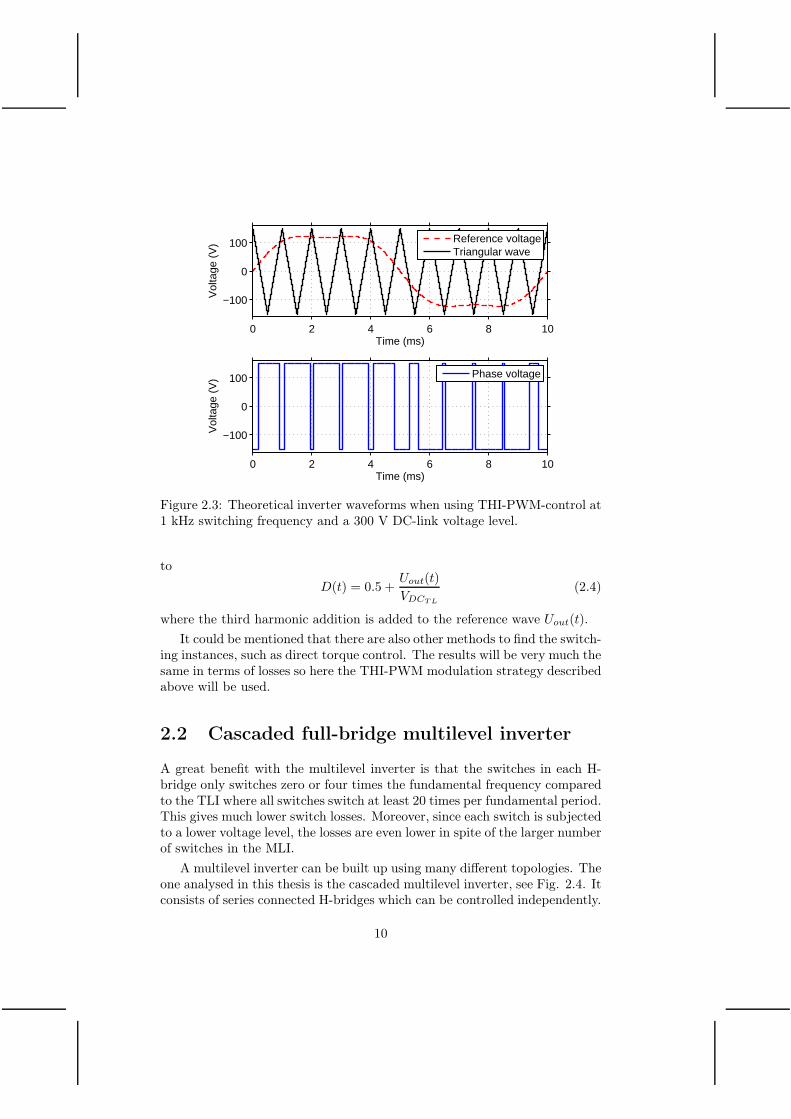
2.1.2 Third harmonic injection(THI)-PWM
When a TLI is controlled in THI-PWM-mode, three voltage references arecreated and compared to a triangular wave with a frequency equal to theswitching frequency in the same way as in the PWM strategy as can be seenin Fig. 2.3. By adding a third harmonic to the voltage references, the neutralpoint of the machine is altered up and down. The machine will not react tothis third harmonic since the neutral point of the machine is not connectedto the inverter neutral point, instead it is the line-to-line voltages that the
8
0 2 4 6 8 10
−100
0
100
Time (ms)
Vol
tage
(V
)
Reference voltageTriangular wave
0 2 4 6 8 10
−100
0
100
Time (ms)
Vol
tage
(V
)
Phase voltage
Figure 2.2: Theoretical inverter waveforms when using PWM-control at 1kHz switching frequency and a 300 V DC-link voltage level.
machine will react to. The advantage is that the DC-bus voltage can beutilized to a higher extent. Also in this case a margin of 10% is used on theoutput voltage to guarantee controllability of the current. The maximum rmsphase motor voltage, with "low-harmonic" free voltages, will then be equalto
UphaseRMSMAXTHI= 0.9
VDCTL√3√2
(2.2)
which is about 15 % higher than the pure sinusoidal PWM strategy with nodrawbacks.
In order to describe the phase voltage used, the modulation index ma istypically utilised. For the two-level inverter the modulation index ma is inthis thesis defined according to
Uphase = maVDCTL√3√2
(2.3)
where ma can go up to 1.0 without entering over modulation. Observe thatthere exists other types of definitions in literature on the modulation index,ma = 1.0 could also correspond to when (2.1) is fulfilled.
Running the inverter with THI-PWM will give a duty cycleD (the ratio ofthe active time between the upper and lower transistor in the leg) according
9
0 2 4 6 8 10
−100
0
100
Time (ms)
Vol
tage
(V
)
Reference voltageTriangular wave
0 2 4 6 8 10
−100
0
100
Time (ms)
Vol
tage
(V
)
Phase voltage
Figure 2.3: Theoretical inverter waveforms when using THI-PWM-control at1 kHz switching frequency and a 300 V DC-link voltage level.
to
D(t) = 0.5 +Uout(t)
VDCTL
(2.4)
where the third harmonic addition is added to the reference wave Uout(t).
It could be mentioned that there are also other methods to find the switch-ing instances, such as direct torque control. The results will be very much thesame in terms of losses so here the THI-PWM modulation strategy describedabove will be used.
2.2 Cascaded full-bridge multilevel inverter
A great benefit with the multilevel inverter is that the switches in each H-bridge only switches zero or four times the fundamental frequency comparedto the TLI where all switches switch at least 20 times per fundamental period.This gives much lower switch losses. Moreover, since each switch is subjectedto a lower voltage level, the losses are even lower in spite of the larger numberof switches in the MLI.
A multilevel inverter can be built up using many different topologies. Theone analysed in this thesis is the cascaded multilevel inverter, see Fig. 2.4. Itconsists of series connected H-bridges which can be controlled independently.
10
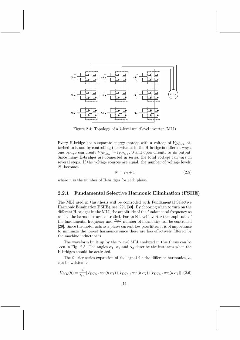
Figure 2.4: Topology of a 7-level multilevel inverter (MLI)
Every H-bridge has a separate energy storage with a voltage of VDCMLat-
tached to it and by controlling the switches in the H-bridge in different ways,one bridge can create VDCML
, −VDCML, 0 and open circuit, to its output.
Since many H-bridges are connected in series, the total voltage can vary inseveral steps. If the voltage sources are equal, the number of voltage levels,N , becomes
N = 2n+ 1 (2.5)
where n is the number of H-bridges for each phase.
2.2.1 Fundamental Selective Harmonic Elimination (FSHE)
The MLI used in this thesis will be controlled with Fundamental SelectiveHarmonic Elimination(FSHE), see [29], [30]. By choosing when to turn on thedifferent H-bridges in the MLI, the amplitude of the fundamental frequency aswell as the harmonics are controlled. For an N-level inverter the amplitude ofthe fundamental frequency and N−3
2 number of harmonics can be controlled[29]. Since the motor acts as a phase current low pass filter, it is of importanceto minimize the lowest harmonics since these are less effectively filtered bythe machine inductances.
The waveform built up by the 7-level MLI analyzed in this thesis can beseen in Fig. 2.5. The angles α1, α2 and α3 describe the instances when theH-bridges should be activated.
The fourier series expansion of the signal for the different harmonics, h,can be written as
UML(h) =4
h π[VDCML
cos(h α1)+VDCMLcos(h α2)+VDCML
cos(h α3)] (2.6)
11

0 π/2 π 3π/2 2π
Vol
tage
Angle [Rad]
←
←
←
α1
α2
α3
3UDC
ML
2UDC
ML
UDC
ML
0
−1UDC
ML
−2UDC
ML
−3UDC
ML
Phase voltagePhase current
Figure 2.5: Simulated phase voltage from 7-level MLI.
according to [29] when assuming that the DC-voltages are equal for all theH-bridges. Setting the amplitude of harmonic 5 and 7 to zero in the aboveequation system, the switching angles and resulting harmonic spectrum canbe calculated for different amplitudes of the fundamental frequency. For theMLI operated with FSHE, the modulation index ma is defined according to
Uphase = maVDCML
· n√2
. (2.7)
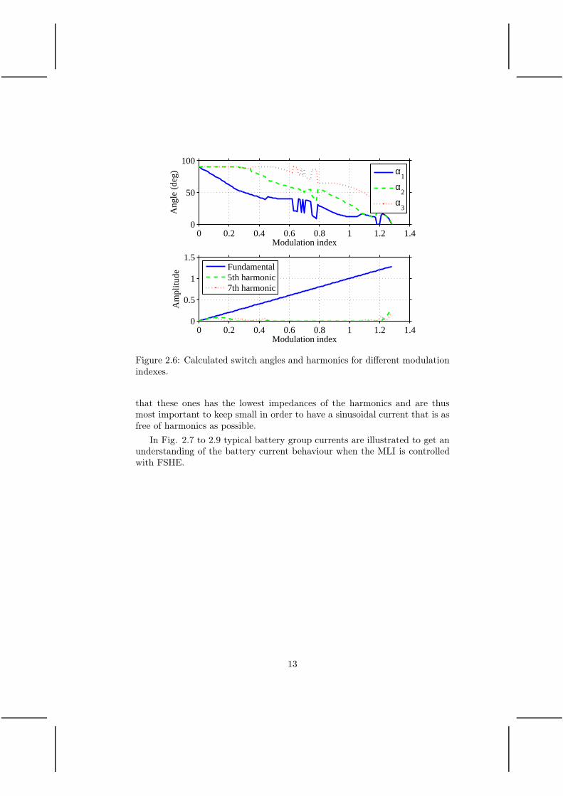
The resulting angles for this case can be seen in Fig. 2.6. The reason forthe discontinuities in the curves are due to that for some operating pointsmore than one solution exist, see [29], and that the solver tracks two differentcurves during the sweep of ma and randomly returns one from each curve.However, it can be seen that the 5th and 7th harmonics are eliminated for allmodulation indexes in this range. The modulation index can go up to 1.07without loosing the control to eliminate the 5th and 7th harmonic. Usinga modulation index below 0.5, the control over the harmonics are also lostbut are minimized with a prioritization on the 5th harmonic. The maximumvoltage the inverter can produce with a margin of 10% can accordingly beexpressed as
UphaseRMS MAX= 0.9 · 1.07VDCML
· n√2
. (2.8)
The reason for selecting the 5th and 7th harmonic to be eliminated is
12
0 0.2 0.4 0.6 0.8 1 1.2 1.40
50
100
Modulation index
Ang
le (
deg)
α
1
α2
α3
0 0.2 0.4 0.6 0.8 1 1.2 1.40
0.5
1
1.5
Modulation index
Am
plitu
de
Fundamental5th harmonic7th harmonic
Figure 2.6: Calculated switch angles and harmonics for different modulationindexes.
that these ones has the lowest impedances of the harmonics and are thusmost important to keep small in order to have a sinusoidal current that is asfree of harmonics as possible.
In Fig. 2.7 to 2.9 typical battery group currents are illustrated to get anunderstanding of the battery current behaviour when the MLI is controlledwith FSHE.
13

0 π/2 π 3π/2 2π
Cur
rent
in b
atte
ry 1
[A]
Angle [Rad]
←
α1
I
0
−I
Battery current without CBattery current with C
Figure 2.7: Theoretical current waveform through the battery module con-trolled with α1.
0 π/2 π 3π/2 2π
Cur
rent
in b
atte
ry 2
[A]
Angle [Rad]
←
α2
I
0
−I
Battery current without CBattery current with C
Figure 2.8: Theoretical current waveform through the battery module con-trolled with α2.
14
0 π/2 π 3π/2 2π
Cur
rent
in b
atte
ry 3
[A]
Angle [Rad]
←
α3
I
0
−I
Battery current without CBattery current with C
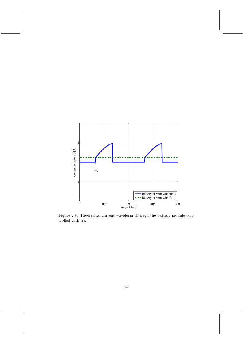
Figure 2.9: Theoretical current waveform through the battery module con-trolled with α3.
15

2.2.2 Balancing strategy for MLI
To ensure that the State of Charge (SOC) is equal among the battery packs,the control system needs to control the use of each H-bridge with respect tothe SOC. By programming the controller to use the battery with the highestvoltage as the one controlled with α1 and the one with the lowest voltagewith α3, the voltage distribution can be kept equal over time.
In the MLI, the balancing between the battery groups comes automati-cally in the control. A small balancing circuit is needed within each batterygroup but this only needs to balance the cells within this group. In the TLI,the balancing has to be done within the whole battery pack where a muchlarger difference in SOC needs to be balanced.
Here a great advantage is that if the cells slowly degrade in a differentpace, they can still be utilised in their own best individual performance withineach battery group. A TLI on the other hand, must always be operated atthe performance level of the most degraded cell.
2.3 Electric machine and torque control
Many different electric machine topologies suitable for EVs exist. The switchedreluctance machine, SRM, is discussed in [31] where it is stated that it canbe a good choice for electrified vehicles, especially for high speeds. How-ever, worries exist that the SRM creates audible noise, so it might not bethe best choice for EVs. The Tesla Roadster uses an asynchronous machine,AM [32]. Both the SRM and the AM are very interesting due to high and un-certain magnetic prices. Another magnet-free candidate is the synchronousreluctance machine [33]. The most commonly used machine is anyway thepermanent magnet synchronous machine, PMSM. Since it is the most com-mon choice it will be the one analyzed in this thesis. Electric machines usedin EVs has to be able to produce enough torque at a large speed range togive a good enough performance to the vehicle. In order to keep the machinesize down it is typically used 2-3 times above its continuous operating ratingfor 5-20 seconds, see [34], [35] and [36].
In order to calculate the losses in the inverter, the waveforms of the cur-rents and voltages to the electric machine need to be known. The electricmachine used in this thesis is a permanent magnet synchronous machine,PMSM, with a different inductance in the d and q direction. This gives thepossibility to produce a reluctance torque as well as a magnetic torque. ThePMSM machine is modeled in steady state with amplitude invariant trans-
16

formations with the following equations when neglecting the magnetic losses,
usd = Rsisd − ωelLqisq (2.9)
usq = Rsisq + ωelLdisq + ωelψm (2.10)
Te =3
2p[ψmisq + (Ld − Lq)isqisd] (2.11)
UphaseRMS=
√
u2sd + u2sq2
(2.12)
IphaseRMS=
√
i2sd + i2sq2
(2.13)
ϕ = ∠ ~us − ∠~is (2.14)
Neglecting the magnetic losses are considered acceptable since the effi-ciency of the electric machine will not be dependant on whether the machineis operated with the TLI or the MLI. It will however affect the operatingpoints for the inverters but only to a minor extent and since it affects theanalysis of both inverters in the same way, it is also considered to be accept-able.
The machine is controlled with MTPA (Maximum Torque Per Ampere)control and with a phase voltage limitation and a current limitation. Whenthe voltage limit is reached, the machine is controlled with field weakeninguntil the maximum current is reached according to the procedure describedin [35]. At the highest speeds the machine might not be able to operateat maximum current depending on the machine parameters, and must theninstead be operated along the maximum torque per voltage line (MTPV) [37].
The chosen current vector when using MTPA is presented in Fig. 2.10.It can be seen that the MTPA line is followed for low speeds (up until almost3000 rpm), but at higher speeds, the field weakening region has to be entered.The higher the speed, the earlier the field weakening region has to be enteredand at 12000 rpm the machine needs to be operated with field weakeningeven at zero current (zero torque) due to the high back EMF that is presentat these high speeds.
2.4 Charger
In [24], different topologies for on board chargers are discussed. An advantagewith an on-board charger is that the already existing propulsion inverter canbe used as a charger. Some topologies even use the inductances in the electricmachine as filter components during charging operation. The requirementsfor a charger for an electric vehicle are widely discussed for instance in [38].
17

−250 −200 −150 −100 −50 0 50 100 150−200
−150
−100
−50
0
50
100
150
2002000 rpm
4000 rpm
6000 rpm 8000 rpm 12000 rpm
isdRMS
(A)
isq R
MS(A
)
Motor operationGenerator operation
Figure 2.10: Resulting current vector when using MTPA.
It is stated that power factor control is needed, as well as the importanceto make sure that the SOC distribution in the battery is constant duringcharging. In the same way as for the TLI, an advantage with the MLI is thatit can be controlled to have a power factor close to unity when rectifying ACto DC during charging operation [39]. In [40] the infrastructure perspectiveof the charging of EVs are discussed, where a need for bidirectional chargersare stated. This functionality comes from the need of the power system.First, the vehicles can act as energy storages, and then secondly, emergencypower can be fed from the vehicles out to the grid if large production unitsshut down. Both the MLI and the TLI systems have this feature. It is shownthat the charger can be built up by already existing components in the EVswith good results, see [41], [42] and [43]. Therefore, using the MLI and theTLI as a charger, as is addressed in this thesis, seems thus to be a beneficialchoice from many perspectives.
To be able to have control over the current during charging, the voltagethe inverter can produce needs to be higher than the grid voltage. In thisthesis, the voltage the inverter can produce is designed to match the selected,rather standard, electric machine and is lower than the grid voltage, hence atransformer is needed for both the TLI and the MLI system. Worth noticingis that this could be redesigned in the future, without any bigger drawback,making it possible to eliminate the transformer. The transformer used in thiswork is modeled as an ideal transformer without losses, see Fig. 2.11. The
18

losses in the transformer are neglected since it is assumed that the currentwaveforms for both the MLI as well as the TLI are almost the same andtherefore the transformer losses will be approximately the same for bothsystems.
For the three phase charging, the transformer is assumed to supply themaximum voltage the inverter can produce, with a margin of 10 %.
GR
ID
IN
VE
RT
ER
VR Grid VR Inverter
VS Grid
VT Grid
VS Inverter
VT Inverter
VN InverterVN Grid
Protective Earth
V
Figure 2.11: Charging transformer.
19

20

Chapter 3
Inverter loss modeling
In order to evaluate the benefits of using a multilevel inverter (MLI) in elec-trified vehicles, it is compared to a reference classical two-level inverter (TLI)system in terms of efficiency. To calculate the losses for different operatingpoints, both models of the inverter components as well as the inverter topolo-gies and control strategies are needed.
3.1 Power electronic components
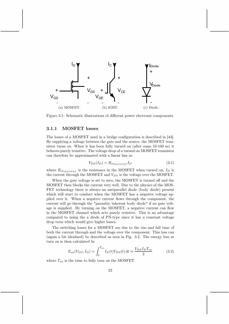
To be able to calculate the losses in different inverter topologies, informationabout the components are needed. In the TLI, IGBTs are used due to theirhigh voltage blocking ability, see Fig. 3.1b, together with diodes, see Fig.3.1c.
In the MLI, MOSFETs will be used due to the lower blocking voltagerequirement for the MLI H-bridge modules, see Fig. 3.1a. This is an impor-tant advantage since MOSFETs usually have much lower losses mainly dueto that they have a purely resistive voltage drop. Moreover, a benefit of aMOSFET is that it has a built in body diode that sometimes is sufficient asa freewheeling diode. In this thesis, this is the case, so no external diodeswill be used in this analysis. In addition, the MOSFETs can conduct in thereverse direction with lower conduction losses than the conduction losses ofa good external diode or its internal body diode.
21
+
VDS
-
+
VGS
-
ID
(a) MOSFET.
+
VCE
-
+
VGE
-
IC
(b) IGBT.
+
V Diode
IDiode
-
(c) Diode.
Figure 3.1: Schematic illustrations of different power electronic components.
3.1.1 MOSFET losses
The losses of a MOSFET used in a bridge configuration is described in [44].By supplying a voltage between the gate and the source, the MOSFET tran-sistor turns on. When it has been fully turned on (after some 10-100 ns) itbehaves purely resistive. The voltage drop of a turned on MOSFET transistorcan therefore be approximated with a linear line as
VDS(ID) = RonMOSFETID (3.1)
where RonMOSFETis the resistance in the MOSFET when turned on, ID is
the current through the MOSFET and VDS is the voltage over the MOSFET.
When the gate voltage is set to zero, the MOSFET is turned off and theMOSFET then blocks the current very well. Due to the physics of the MOS-FET technology there is always an antiparallel diode (body diode) presentwhich will start to conduct when the MOSFET has a negative voltage ap-plied over it. When a negative current flows through the component, thecurrent will go through the "parasitic/inherent body diode" if no gate volt-age is supplied. By turning on the MOSFET, a negative current can flowin the MOSFET channel which acts purely resistive. This is an advantagecompared to using the a diode of PN-type since it has a constant voltagedrop term which would give higher losses.
The switching losses for a MOSFET are due to the rise and fall time ofboth the current through and the voltage over the component. This loss can(again a bit idealized) be described as seen in Fig. 3.2. The energy loss atturn on is then calculated by
Eon(VDS , ID) =
∫ Ton
0
ID(t)VDS(t) dt ≈VDSIDTon
2(3.2)
where Ton is the time to fully turn on the MOSFET.
22

The energy loss at turn off will in the same way be equal to
Eoff (VDS , ID) =
∫ Toff
0
ID(t)VDS(t) dt ≈VDSIDToff
2(3.3)
where Toff is the time to fully turn off the MOSFET.
0 10 20 30 40 50 60 700
50
100
150
Time (ns)
VD
S, ID
vDS
ID
0 10 20 30 40 50 60 70
0
5
10
Time (ns)
P loss
[kW
]
Figure 3.2: Simplified illustration of the turn on losses for MOSFET, switch-ing times approximated for a 100 V MOSFET.
Although the switching waveforms in a MOSFET are simpler to describethan those of the IGBT, they are still very hard to describe, not only dueto the mathematical description, but also since circuit and component par-asitics strongly influence the behaviour. In this work, this is no problemsince the switching frequency is very low, so switching losses give a marginalcontribution to the total losses.
3.1.2 IGBT losses
The losses in an IGBT are described in [45] when used in a bridge configura-tion. It is often assumed that the voltage drop of the IGBT is approximatedwith two straight lines when it is operated in on-state. The two lines areexpressed as
VCE(IC) = VtIGBT+ RonIGBT
IC IC > 0
IC = 0 VCE < VtIGBT(3.4)
23

0 50 100 150 2000
50
100
150
200
250
Time (ns)
VC
E, IC
vCE
IC
0 50 100 150 2000
10
20
30
40
Time (ns)
P loss
[kW
]
Figure 3.3: Simplified illustration of the turn on loss for an IGBT, switchingtimes approximated for a 600 V IGBT.
where RonIGBTis the resistance when fully turned on, VtIGBT
is the constantvoltage drop in the IGBT, IC is the current through the IGBT and VCE isthe voltage over the IGBT.
When turned off, the IGBT current becomes
IC = 0. (3.5)
The switching losses for an IGBT occur when switching from the on stateto the off state and vice versa. During the time the IGBT is switching, theoccurrence of both voltage and current is present in and over the device whichis causing a much higher power loss compared to when the IGBT is in theon state. However, the time when this power loss occurs is very short butsince it occurs around 10 000 times every second, it greatly contributes tothe inverter losses. This phenomena can (a bit idealized) for a turn on of theIGBT be seen in Fig. 3.3.
The energy loss at turn on is then for this simplified case calculated as
Eon(VCE , IC) =
∫ Ton
0
IC(t)VCE(t) dt ≈VCEICTon
2(3.6)
where Ton is the time to fully turn on the IGBT.
The energy loss at turn off can in the same way be roughly approximated
24
as
Eoff (VCE , IC) =
∫ Toff
0
IC(t)VCE(t) dt ≈VCEICToff
2(3.7)
where Toff is the time to fully turn off the IGBT.
However, in reality the switching losses can not be accurately predictedusing algebraic expressions, not even sufficiently using even more complexity.Therefore, if more accurate results are needed, tables from the data sheetsare commonly used. In the data sheet, the switching loss is usually plottedas a function of current at a certain blocking voltage. When linearising thisloss it can be written as
Eon(VCE , IC) = KonVCEIC (3.8)
andEoff (VCE , IC) = KoffVCEIC (3.9)
where Kon and Koff are the parameters that describe the linearisation ofthe data sheet.
If (3.6) and (3.8) are compared and (3.7) and (3.9) are compared, it canbe noticed that the parameters Ton and Toff can be calculated from the datasheets according to
Ton = 2Kon (3.10)
andToff = 2Koff . (3.11)
In this work the dc-link voltage is always constant, if the dc-link voltagevaries, it is a good idea to modify (3.6) and (3.7) with a non-linear voltageterm, since the switching losses rise more than linearly as a function of dc-linkvoltage level.
3.1.3 Diode losses
The losses of a diode used in a bridge configuration is discussed in both [45]and in [44]. The voltage drop of the diode is approximated with two straightlines as
VDiode(IDiode) = VtDiode+RDiodeIDiode IDiode > 0
IDiode = 0 VDiode < VtDiode(3.12)
where RDiode is the resistance in the diode, VtDiodeis the constant voltage
drop in the diode (typically around 1 V), IDiode is the current through the
25

diode and VDiode is the voltage over the diode between the anode and thecathode.
The switching loss of a diode is assumed to be zero at turn on since itis very low [45], but at turn off the diode has to deplete the charges thatare stored in the junction from when it vas forward biased. This will createa current in the reverse direction for a short period of time and the energythat is released becomes a loss in both the diode and the opposing switchwhen connected in a leg configuration. The charge that has to be depletedis current dependent and is for simplicity assumed to be proportional to thecurrent that flew in the diode at the instant right before turn off. The totalenergy loss can according to [45] be written as
ERR =QrrVdrr
4=Qrr(−VDiode)
4(3.13)
where Qrr is the charge stored in the diode at the time of the reverse recovery.
If the charge that is stored in the diode can be considered to be pro-portional to the current, the reverse recovery energy loss can be rewrittenas
ERR = Krr(−VDiode)IDiode (3.14)
where Krr is the loss factor. The loss factor Krr is taken from the datasheet where the reverse recovery loss is often specified at a certain blockingvoltage and current. Sometimes, they are also specified for a certain currentderivative.
Again, in reality, ERR is a complicated parameter to determine and datasheets values with non-linear relations are typically used. However, for theloss calculations made in this thesis, (3.14) is used.
3.1.4 Miscellaneous power electronic components
Other components in the inverter also affect the losses in the power train.Here, they are assumed ideal but for example a bad PCB design can have aninfluence on the losses. To switch the transistors, a driver circuit is needed.In the following work the driver circuit for the transistors is assumed to belossless. Also, the losses in the dc-link capacitors are ignored, except forChapter 7.
3.2 Two level inverter (TLI)
To be able to calculate the losses in the TLI, information about the operatingpoints used and the control strategy used is needed. The TLI will in this
26
analysis be controlled with THI-PWM. The reference output voltage for thefirst phase is described as
Vout(t) = U [sin(ωt+ ϕ) + a sin(3ωt+ 3ϕ)] (3.15)
and the current asIout(t) = I sin(ωt) (3.16)
where U is the amplitude of the phase voltage, ω is the electric frequency, ϕis the phase difference between voltage and current and I is the amplitudeof the phase current. The amplitude of the third harmonic component ashould be selected to 0.19 for maximum utilization of the DC-voltage, [46].Although a slightly higher modulation can be reached by using more har-monic components on the reference wave, (3.15) is the wave-shape used forthe loss determination in this thesis.
3.2.1 Conduction losses
The losses are calculated for one phase of the inverter and are then scaled tobe valid for three phases. During the time when the current is positive, thecurrent will go through IGBT1H and Diode1L, see Fig. 2.1. The losses in theother pair, IGBT1L and Diode1H , will be equal to the loss in the first pairwhen the current is negative. If the frequency of the sine wave is assumed tobe much smaller than the switching frequency, the current and the referencevoltage can be assumed to be constant during one switching period. Theaverage conduction loss for one switching event in IGBT1H and Diode1L canthen be expressed as
PcondIGBT1H(Iout, D) =
1
Tsw
∫ Tsw
0
VDS(ID)ID dt =
DIoutVtIGBT+DRonIGBT
I2out (3.17)
and
PcondDiode1L(Iout, D) =
1
Tsw
∫ Tsw
0
VDiode(IDiode)IDiode dt =
(1−D)IoutVtDiode+ (1 −D)RonDiode
I2out (3.18)
using (3.4) and (3.12).
To calculate the average conduction losses for one phase, one can chooseto study the positive part of the current, knowing that the current onlygoes through IGBT1H and Diode1L. Knowing that the same losses will begenerated in IGBT1L and Diode1H during the negative part of the current,
27

the average losses of one leg can then, by combining (3.17) and (2.4), bewritten as
PconductionIGBTs1=
∫ Tf
0 PcondIGBT1H(t) + PcondIGBT1L
(t) dt
Tf=
∫ Tf/2
0PcondIGBT1H
(t) dt
Tf/2=
IVtIGBT(1
π+U cosϕ
2VDCTL
) +RonIGBTI2(
1
4+
4U cosϕ
3πVDCTL
− 2a · cos(3ϕ)15π
). (3.19)
The losses in the diode can be calculated in the same way using (3.18)and (2.4) which gives
PconductionDiodes1=
∫ Tf
0 PcondDiode1H(t) + PcondDiode1L
(t) dt
Tf=
∫ Tf/2
0PcondDiode1L
(t) dt
Tf/2=
IVtDiode(1
π− U cosϕ
2VDCTL
) +RonDiodeI2(
1
4− 4U cosϕ
3πVDCTL
+2a · cos(3ϕ)
15π). (3.20)
3.2.2 Switching losses
The switching losses for the IGBTs can be calculated with the assumptionthat the fundamental frequency is much lower than the switching frequency.If the leg would operate in DC-mode, the average switching loss for IGBT1Hcan be described as
PswitchIGBT1H(Iout) = [Eon(Iout) + Eoff (Iout)]fsw =
(Ton + Toff)VDCTLIoutfsw
2. (3.21)
For the diodes, the turn on losses are neglected but the reverse recoverycan have a significant contribution to the losses. It can be written as
PrrDiode1L(Iout) = Err(Iout)fsw = KrrVDCTL
Ioutfsw (3.22)
using (3.14).
28

Operating the converter in AC mode, the switch losses for the IGBTs inone leg can then be calculated as
PswitchIGBTs1=
∫ Tf/2
02(Ton+Toff )VDCTL
Iout(t)fsw2 dt
Tf=
2(Ton + Toff)VDCTLfsw ˆIout
π(3.23)
and the diode losses as
PrrDiodes1=
∫ Tf/2
02KrrVDCTL
Iout(t)fsw dt
Tf=
2KrrVDCTLˆIoutfsw
π. (3.24)
3.2.3 Total losses
The total losses for a TLI running in AC-mode will therefore be the sum ofthe losses in one leg multiplied with the number of legs which gives
PLossTLI= 3(PconductionIGBTs1
+ PconductionDiodes1+
PswitchIGBTs1+ PrrDiodes1
) (3.25)
using (3.19), (3.20), (3.23) and (3.24).
3.3 Multilevel inverter (MLI)
To be able to calculate the losses in the MLI, information about the operatingpoint is needed as well as the control strategy. In this analysis, it will becontrolled with Fundamental Selective Harmonic Elimination, FSHE. TheMLI is assumed to be operating at an output voltage expressed as
Vout(t) = U(sin(ωt+ ϕ)) (3.26)
and the current asIout(t) = I sin(ωt). (3.27)
3.3.1 Conduction losses
The current will always flow through two transistors for each H-bridge. Thevoltage drop for one MOSFET can be written according to (3.1). The totalvoltage drop will therefore be equal to
Vdrop = 2nIout(t)RonMOSFET(3.28)
29

independently of the current direction assuming that the MOSFET is turnedon when conducting in the reverse direction.
The conduction power loss for all three phases of the MLI can thereforebe calculated as
PconductionMLI= 6nI2outRMS
RonMOSFET= 3nI2RonMOSFET
. (3.29)
3.3.2 Switching losses
The switching losses can be described as a sum of the energy losses duringone cycle. When controlled with FSHE, the switching occurs very seldom, seeFig. 2.5. During the first three switching instances, the inverter switches theH-bridges to create a positive voltage. Depending on the current directionthis will result in either a turn on or a turn off loss. The loss for the MOSFETand diode can therefore at the first three switching instances be written as
Eonα1,2,3=VdcML
I(α1,2,3)Ton2
I(α1,2,3) ≥ 0
Eonα1,2,3= 0 I(α1,2,3) < 0 (3.30)
Eoffα1,2,3= 0 I(α1,2,3) ≥ 0
Eoffα1,2,3=VdcML
I(α1,2,3)Toff2
I(α1,2,3) < 0 (3.31)
Errα1,2,3= VdcML
I(α1,2,3)Krr I(α1,2,3) ≥ 0
Errα1,2,3= 0 I(α1,2,3) < 0. (3.32)
For the fourth, fifth and sixth switching instances the inverter switchesto create zero volts for the inverters. This gives a loss according to
Eonα4,5,6= 0 I(α4,5,6) ≥ 0
Eonα4,5,6=VdcML
I(α4,5,6)Ton2
I(α4,5,6) < 0 (3.33)
Eoffα4,5,6=VdcML
I(α4,5,6)Toff2
I(α4,5,6) ≥ 0
Eoffα4,5,6= 0 I(α4,5,6) < 0 (3.34)
Errα4,5,6= 0 I(α4,5,6) ≥ 0
Errα4,5,6= VdcML
I(α4,5,6)Krr I(α4,5,6) < 0. (3.35)
During switching occasion 7 to 12 the losses will be equal to the lossduring switch 1 to 6. Therefore the losses can be calculated as
PswitchMLI= 3 · 2 · ffund
6∑
n=1
(Eonαn+ Eoffαn
+ Errαn). (3.36)
30

3.3.3 Total losses
The total losses for the multilevel inverter can be written as
PLossML= PconductionMLI
+ PswitchMLI(3.37)
using (3.29) and (3.36).
31

32
Chapter 4
Case setup & inverter
waveform verification
To make a comparison between the TLI and the MLI, some boundary con-ditions has to be established. This chapter presents the chosen componentsnecessary to build up the drive system as well as defining appropriate oper-ating conditions for performing energy consequence studies. For the furtheranalysis, a 25 C temperature is assumed unless otherwise stated.
First, the system used for the main analysis is presented Section 4.1. Thenthe experimental small scale system is described in Section 4.2 and used inSection 4.3 for a verification of the theory from Chapter 2.
4.1 Small PEV reference vehicle
The vehicle analyzed is a small compact PEV with the data given in Table4.1. It is made small to match the rating of the electric machine so thatall operating points for the analysed drive cycles can be achieved. It hasan electric driving range of around 50 km, but some analysis is later madewith the same vehicle but a four times bigger battery size. In this thesis, thevehicle does not incorporate regenerative breaking. However, since all theanalysis is done in the same way the differences between various results areconsidered to be valid.
33

Table 4.1: Car parameters.
Parameter Value Unit
Weight 1100 kgA · Cd 0.45 Nv−2
Friction coefficient 0.01 NWheel radius 0.33 mGearbox ratio 11.5Gearbox efficiency 90 %Top speed 130 kmh−1
4.1.1 Electric machine
The electric machine used for the analysis in this thesis is a PMSM machinewith parameters according to Table 4.2. The magnetic losses have beenignored.
Table 4.2: Parameters of the electric machine.
Parameter Value Unit
Ld 150 µHLq 300 µHRs 20 mΩPole pairs 5ψm 33 mWbMaximum transient phase voltage 106 VRMS
Maximum transient phase current 212 ARMS
Maximum transient torque 109 NmMaximum transient power 49 kW
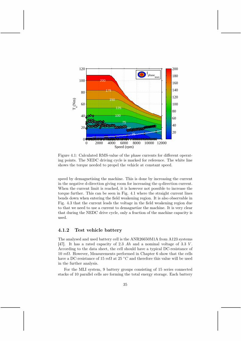
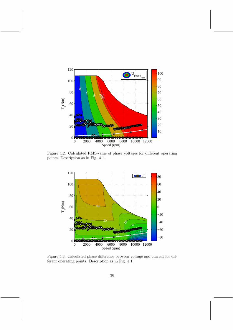
Operating the electric machine at different torques and speeds gives theoperation points according to Fig. 4.1 to 4.3 using (2.9) to (2.14) when usinga DC-voltage of 260 V to account for control margin and battery voltage drop.In the figures, the operation points of the NEDC drive cycle (which will bepresented in section 4.1.5) is also given as a reference of where the electricmachine is typically used. In Fig. 4.2 it can be seen that the voltage increaseswith speed up to the field weakening region. When the maximum voltagegoverned by the battery is reached, the machine can continue to increase its
34
Speed (rpm)
Te(N
m)
200
175
150
125
100
75
50
25
0 2000 4000 6000 8000 10000 120000
20
40
60
80
100
120
20
40
60
80
100
120
140
160
180
200Iphase
RMS
Figure 4.1: Calculated RMS-value of the phase currents for different operat-ing points. The NEDC driving cycle is marked for reference. The white lineshows the torque needed to propel the vehicle at constant speed.
speed by demagnetising the machine. This is done by increasing the currentin the negative d-direction giving room for increasing the q-direction current.When the current limit is reached, it is however not possible to increase thetorque further. This can be seen in Fig. 4.1 where the straight current linesbends down when entering the field weakening region. It is also observable inFig. 4.3 that the current leads the voltage in the field weakening region dueto that we need to use a current to demagnetize the machine. It is very clearthat during the NEDC drive cycle, only a fraction of the machine capacity isused.
4.1.2 Test vehicle battery
The analysed and used battery cell is the ANR26650M1A from A123 systems[47]. It has a rated capacity of 2.3 Ah and a nominal voltage of 3.3 V .According to the data sheet, the cell should have a typical DC-resistance of10 mΩ. However, Measurements performed in Chapter 6 show that the cellshave a DC-resistance of 15 mΩ at 25 C and therefore this value will be usedin the further analysis.
For the MLI system, 9 battery groups consisting of 15 series connectedstacks of 10 parallel cells are forming the total energy storage. Each battery
35
Speed (rpm)
Te(N
m)
25
50 75 100106
0 2000 4000 6000 8000 10000 120000
20
40
60
80
100
120
10
20
30
40
50
60
70
80
90
100Uphase
RMS
Figure 4.2: Calculated RMS-value of phase voltages for different operatingpoints. Description as in Fig. 4.1.
Speed (rpm)
Te(N
m)
40
30
20 20
10
10
0−10
−20
0 2000 4000 6000 8000 10000 120000
20
40
60
80
100
120
−80
−60
−40
−20
0
20
40
60
80ϕ
Figure 4.3: Calculated phase difference between voltage and current for dif-ferent operating points. Description as in Fig. 4.1.
36
group will have a nominal voltage of 49.5 V . The nominal energy content ofall 9 groups sums up to a total capacity of 10.25 kWh.
For the TLI system, one big battery pack is formed consisting of 90 seriesconnected stacks of 15 parallel connected cells, building up a total capacityof 10.25 kWh at a nominal voltage of 297 V .
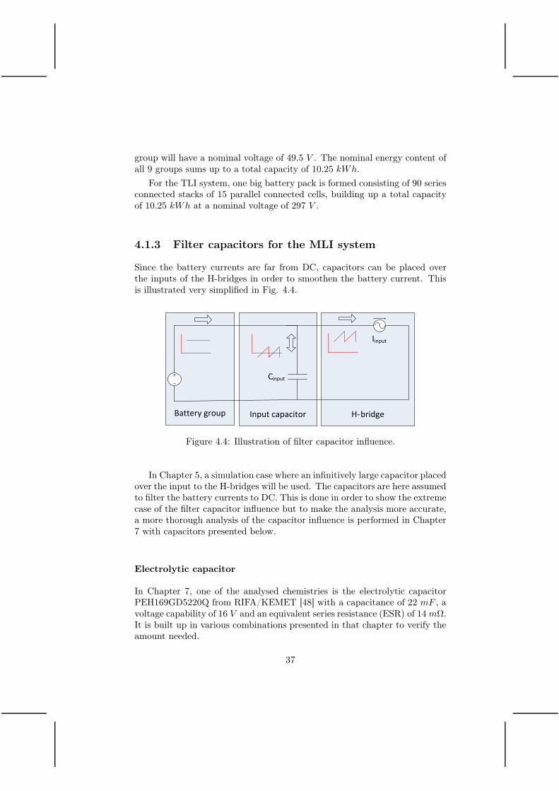
4.1.3 Filter capacitors for the MLI system
Since the battery currents are far from DC, capacitors can be placed overthe inputs of the H-bridges in order to smoothen the battery current. Thisis illustrated very simplified in Fig. 4.4.
Input capacitor
Cinput
H-bridge
Iinput
Battery group
Figure 4.4: Illustration of filter capacitor influence.
In Chapter 5, a simulation case where an infinitively large capacitor placedover the input to the H-bridges will be used. The capacitors are here assumedto filter the battery currents to DC. This is done in order to show the extremecase of the filter capacitor influence but to make the analysis more accurate,a more thorough analysis of the capacitor influence is performed in Chapter7 with capacitors presented below.
Electrolytic capacitor
In Chapter 7, one of the analysed chemistries is the electrolytic capacitorPEH169GD5220Q from RIFA/KEMET [48] with a capacitance of 22 mF , avoltage capability of 16 V and an equivalent series resistance (ESR) of 14mΩ.It is built up in various combinations presented in that chapter to verify theamount needed.
37
Super capacitor
The second chemistry analysed in Chapter 7 is the super capacitor. It isin that analysis built up by different combinations of the super capacitorRSC2R7107SR from Ioxus [49] with a capacitance of 100 F , a voltage capa-bility of 2.7 V and an ESR of 4.6 mΩ. In the same way as for the electrolyticcapacitor, the capacitor is scaled to various amounts to look at the capacitorinfluence.
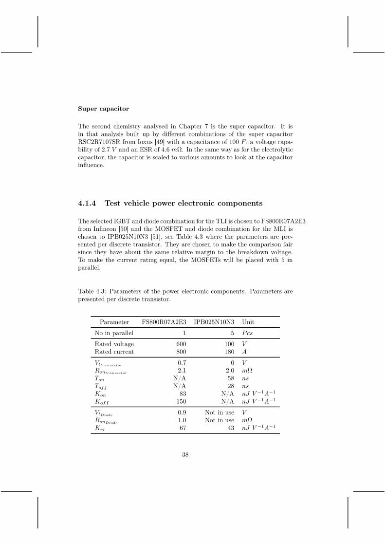
4.1.4 Test vehicle power electronic components
The selected IGBT and diode combination for the TLI is chosen to FS800R07A2E3from Infineon [50] and the MOSFET and diode combination for the MLI ischosen to IPB025N10N3 [51], see Table 4.3 where the parameters are pre-sented per discrete transistor. They are chosen to make the comparison fairsince they have about the same relative margin to the breakdown voltage.To make the current rating equal, the MOSFETs will be placed with 5 inparallel.
Table 4.3: Parameters of the power electronic components. Parameters arepresented per discrete transistor.
Parameter FS800R07A2E3 IPB025N10N3 Unit
No in parallel 1 5 Pcs
Rated voltage 600 100 VRated current 800 180 A
Vttransistor0.7 0 V
Rontransistor2.1 2.0 mΩ
Ton N/A 58 nsToff N/A 28 nsKon 83 N/A nJ V −1A−1
Koff 150 N/A nJ V −1A−1
VtDiode0.9 Not in use V
RonDiode1.0 Not in use mΩ
Krr 67 43 nJ V −1A−1
38

4.1.5 Drive cycle presentation
When analyzing energy consumption of vehicles in various driving situations,different drive cycles are used in order to perform comparisons. In this thesis,four different drive cycles are used, see Fig. 4.5 and Table 4.4. The drivecycles are used to determine the losses in both the battery and in the inverter,in order to evaluate the performance over a range of operating points.
The first is the New European Driving Cycle, NEDC. The NEDC is de-signed to represent the way vehicles are used in Europe and was introduced1990. It is made up from four repetitions of the city drive cycle ECE15,and one high speed drive cycle, EUDC. The average speed of the vehicle is33 km/h and the maximum speed is 120 km/h. This drive cycle is typicallyused to classify the fuel consumption i Europe, however, the drive cycle hasreceived much critic lately since it does not represent the way cars are used.Modern vehicles have much more power than 20 years ago and are drivenwith steeper accelerations.
The second drive cycle is the EPA Federal Test Procedure, FTP75. Thisdrive cycle is used in the United states to specify the fuel consumption of avehicle. It has the same average speed as NEDC but the top speed is muchlower, only 91 km/h. This drive cycle has also gotten criticism for not beingaggressive enough and is therefore complimented with the US06, describedmore below.
The third drive cycle analyzed is the EPA Highway Fuel Economy Cycle,HWFET. This drive cycle aims at light duty trucks and is included in thisthesis to show the behavior of the multilevel inverter for small trucks. TheHWFET is a much less dynamic drive cycle than the other.
The last drive cycle is the US06 Supplemental Federal Test Procedure,US06. It is a very aggressive drive cycle compared to the others; the accel-erations are harder and the top speed goes up to 129 km/h. It is used as acompliment to the FTP75 to show a more realistic way of the usage of thevehicle.
4.2 Experimental system
To verify the waveforms created by the MLI an experimental setup is de-signed. The inverter will be used to verify the wave shapes used in theanalytical analysis. The experimental MLI can be seen in Fig. 4.6. In theexperimental MLI, the MOSFET IRF1324S-7PPbF from Infineon is used [52].The on resistance (RonMOSFET
) of this MOSFET is only maximum 1 mΩ.
39

0 200 400 600 800 1000 1200 1400 1600 18000
50
100
Time (s)
NE
DC
(km
/h)
0 200 400 600 800 1000 1200 1400 1600 18000
50
100
Time (s)
FT
P75
(km
/h)
0 200 400 600 800 1000 1200 1400 1600 18000
50
100
Time (s)
HW
FE
T (
km/h
)
0 200 400 600 800 1000 1200 1400 1600 18000
50
100
Time (s)
US
06 (
km/h
)
Figure 4.5: Speed profiles of the drive cycles.
Table 4.4: Drive cycle parameters
Drive Speed Speed Time Distance Energy Energycycle avg max regen no regen
[km/h] [km/h] [s] [km] [Wh/km] [Wh/km]
NEDC 33 120 1180 10.9 54 82FTP75 34 91 1874 17.8 44 80HWFET 78 96 766 16.5 68 76US06 78 129 596 12.9 83 117
40

Figure 4.6: Laboratory setup of the 7-level multilevel inverter. The 3 phasesconsist of 3 H-bridges each. The battery inputs are shown in the upper partof the picture, the outputs are on the right side of the groups and the commonY-connection point is shown on the left side of each phase leg.
To each input the same battery cell as for the test vehicle presented inSection 4.1.2 is used, but here only 4 cells are connected in series and 1 inparallel.
As an inverter load, both a small asynchronous machine as well as acontrollable RL-load is used.
4.3 Experimental base verification
4.3.1 Output waveforms and harmonics
Figs. 4.7 to 4.9 show the output voltage from the MLI at ma = 0.5, ma =1.0 and ma = 1.2. It can be seen that the first harmonic in the line toline voltage is number 11 for ma = 0.5 and ma = 1.0. Accordingly theharmonic elimination strategy is fully successful for the first to cases. Whenoperating at ma = 1.2 the possibility to eliminate harmonic 5 and 7 is nolonger present. The result is clearly visible in the measured curves where aset of low-frequency harmonic now have emerged, as can be noted in Fig. 4.9.
41

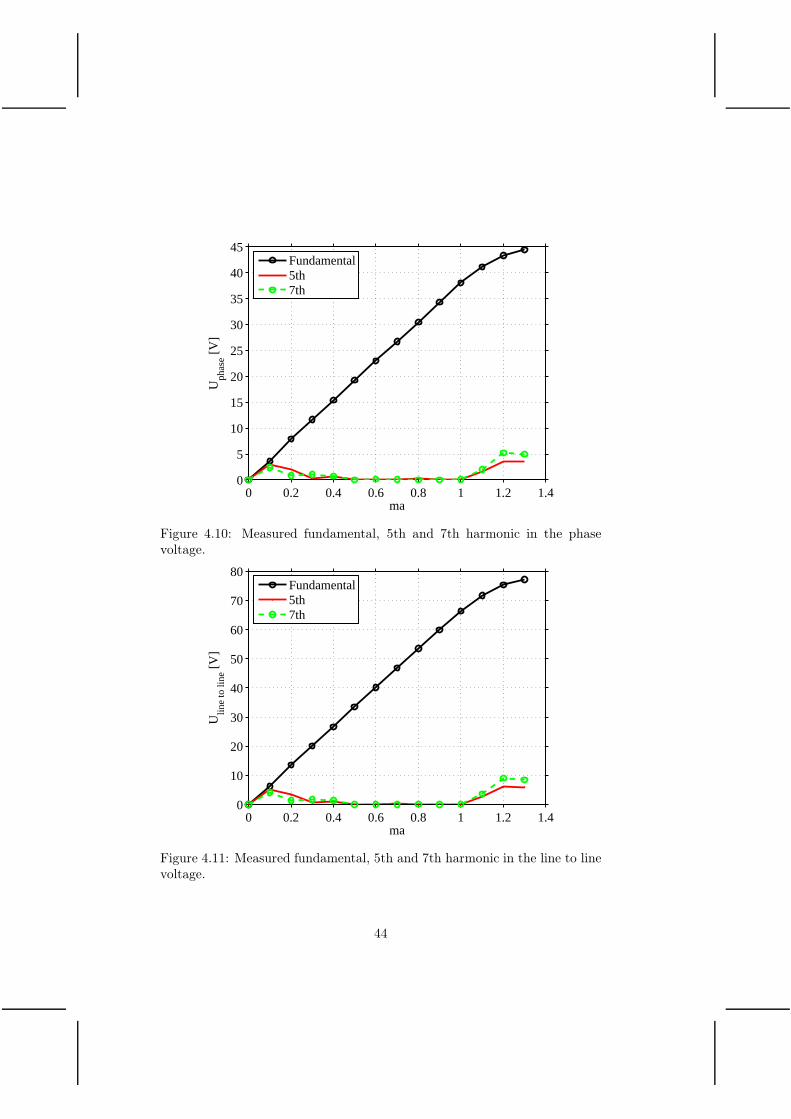
In Fig. 4.10 and 4.11 the 5th and the 7th harmonic are plotted for differentma. It shows a good match with the analytical calculations presented in Fig.2.6.
0 π/2 π 3π/2 2π−50
0
50
Time [s]
Uph
ase
0 10 200
10
20
30
40
50
Harmonic [n]U
phas
e
0 π/2 π 3π/2 2π
−50
0
50
Time [s]
Ulin
e to
line
0 10 200
20
40
60
80
Harmonic [n]
Ulin
e to
line
Figure 4.7: Measured voltage output and harmonic content at ma = 0.5.Dashed lines show the fundamental components. The load is a resistor witha resistance of 1 kΩ.
42

0 π/2 π 3π/2 2π−50
0
50
Time [s]
Uph
ase
0 10 200
10
20
30
40
50
Harmonic [n]
Uph
ase
0 π/2 π 3π/2 2π
−50
0
50
Time [s]
Ulin
e to
line
0 10 200
20
40
60
80
Harmonic [n]
Ulin
e to
line
Figure 4.8: Measured voltage output and harmonic content at ma = 1.0.Dashed lines show the fundamental components. The load is a resistor witha resistance of 1 kΩ.
0 π/2 π 3π/2 2π−50
0
50
Time [s]
Uph
ase
0 10 200
10
20
30
40
50
Harmonic [n]
Uph
ase
0 π/2 π 3π/2 2π
−50
0
50
Time [s]
Ulin
e to
line
0 10 200
20
40
60
80
Harmonic [n]
Ulin
e to
line
Figure 4.9: Measured voltage output and harmonic content at ma = 1.2.Dashed lines show the fundamental components. The load is a resistor witha resistance of 1 kΩ.
43
0 0.2 0.4 0.6 0.8 1 1.2 1.40
5
10
15
20
25
30
35
40
45
ma
Uph
ase [V
]
Fundamental5th7th
Figure 4.10: Measured fundamental, 5th and 7th harmonic in the phasevoltage.
0 0.2 0.4 0.6 0.8 1 1.2 1.40
10
20
30
40
50
60
70
80
ma
Ulin
e to
line
[V]
Fundamental5th7th
Figure 4.11: Measured fundamental, 5th and 7th harmonic in the line to linevoltage.
44
4.3.2 Total Harmonic Distortion
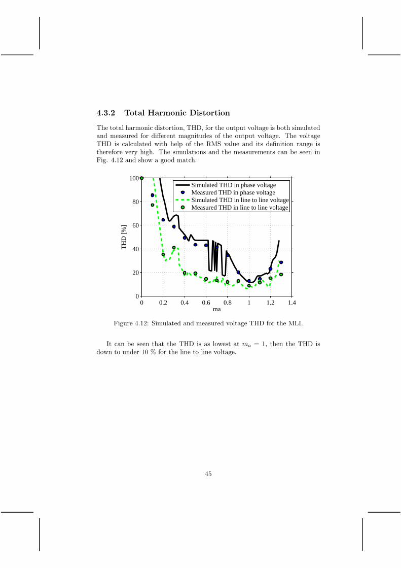
The total harmonic distortion, THD, for the output voltage is both simulatedand measured for different magnitudes of the output voltage. The voltageTHD is calculated with help of the RMS value and its definition range istherefore very high. The simulations and the measurements can be seen inFig. 4.12 and show a good match.
0 0.2 0.4 0.6 0.8 1 1.2 1.40
20
40
60
80
100
ma
TH
D [%
]
Simulated THD in phase voltageMeasured THD in phase voltageSimulated THD in line to line voltageMeasured THD in line to line voltage
Figure 4.12: Simulated and measured voltage THD for the MLI.
It can be seen that the THD is as lowest at ma = 1, then the THD isdown to under 10 % for the line to line voltage.
45

4.3.3 Balancing using the experimental setup
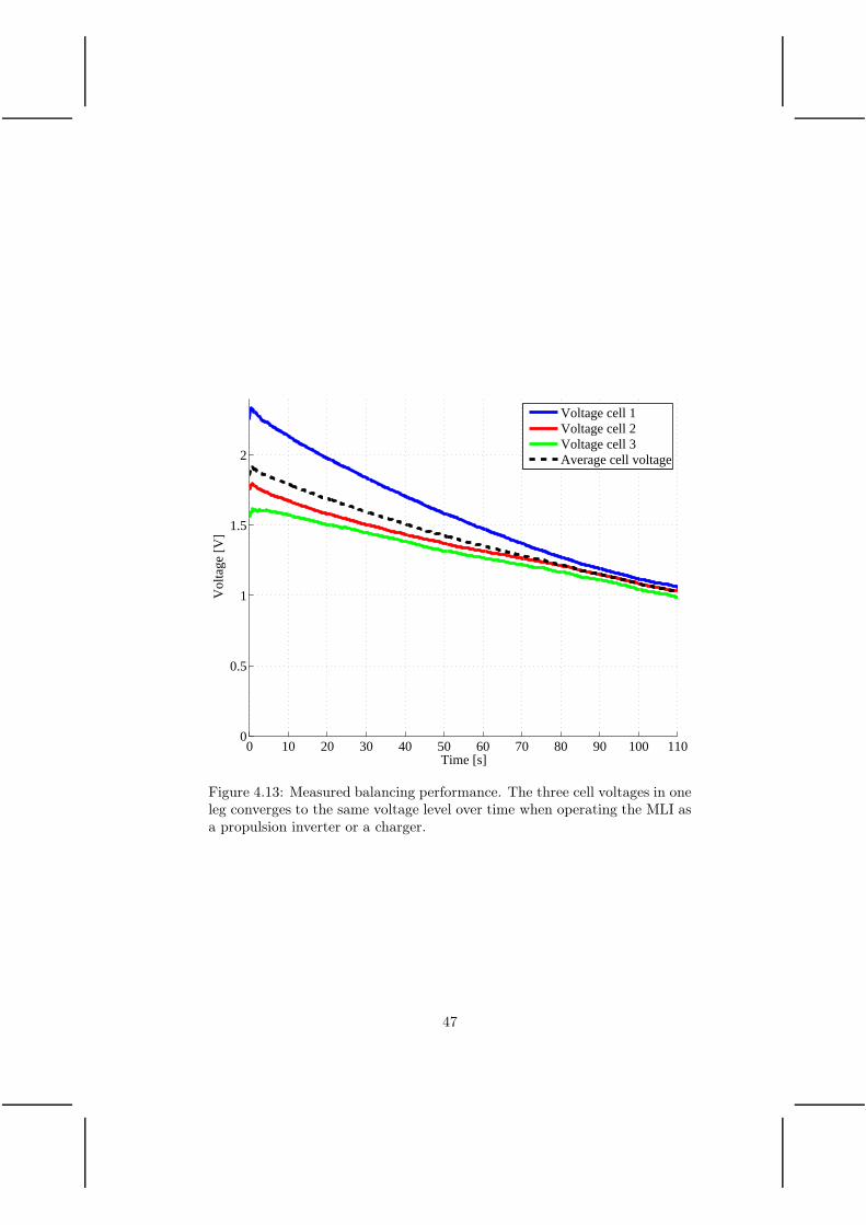
The possibility to balance the battery cells is evaluated with the MLI ex-perimental setup. For this test, the energy sources is chosen to small supercapacitors with a capacitance of 10 F each in order to quickly see the balanc-ing behaviour. The three capacitors in one leg are charged to 1.6 V , 1.8 Vand 2.3 V . The inverter is then operated at ma = 1 to a resistive load toverify that the inverter will balance the cells during sine wave operation. Itis operated at ma = 1 since this case uses all cells most equal amount and istherefor the most demanding case. The control strategy is to use the inverterwith the highest voltage as the inverter controlled with α1, and the inverterwith the lowest voltage as the one controlled with α3.
In Fig. 4.13 the super capacitor voltages are plotted over time, it canbeen seen that the capacitors will have about the same voltage after around90 s. It can also be noted that the voltages never get exactly the same. Thereason for this is that the resolution of the A/D-converters are very poor.For this specific test, when the control system measures that the cells areequal (balanced), it always uses the first H-bridge (green curve) which is theone that is controlled with α1 (since this H-bridge has to output power thelongest time), the second (red curve) with α2 and the third (blue curve) withα3.
This unfortunately causes the cells to never be totally balanced in thissetup, they will stay unbalanced to a level matching the resolution of theA/D-converter. Anyway, up until the A/D-conversion limit, the balancingworks very well.
46
0 10 20 30 40 50 60 70 80 90 100 1100
0.5
1
1.5
2
Vol
tage
[V]
Time [s]
Voltage cell 1Voltage cell 2Voltage cell 3Average cell voltage
Figure 4.13: Measured balancing performance. The three cell voltages in oneleg converges to the same voltage level over time when operating the MLI asa propulsion inverter or a charger.
47

4.3.4 Battery current verification with the experimentalsetup
In Fig. 4.14 the inverter is operated at ma = 1 and ffundamental = 50 Hz.The load consists of an RL load with R = 11 Ω and L = 36 mH . The currentin the battery groups can be seen in Fig. 4.15 to 4.17. These waveforms canbe compared with the theoretical ones presented in Fig. 2.7 to 2.9. Byperforming this comparison, it can be noted that the agreement is very good.
0 π/2 π 3π/2 2π−40
−20
0
20
40
Vol
tage
[V]
Angle [rad]0 π/2 π 3π/2 2π
−4
−2
0
2
4
Cur
rent
[A]
Figure 4.14: Measured output phase voltage and current. Solid blue curveshows the voltage and the green dashed curve shows the current.
48
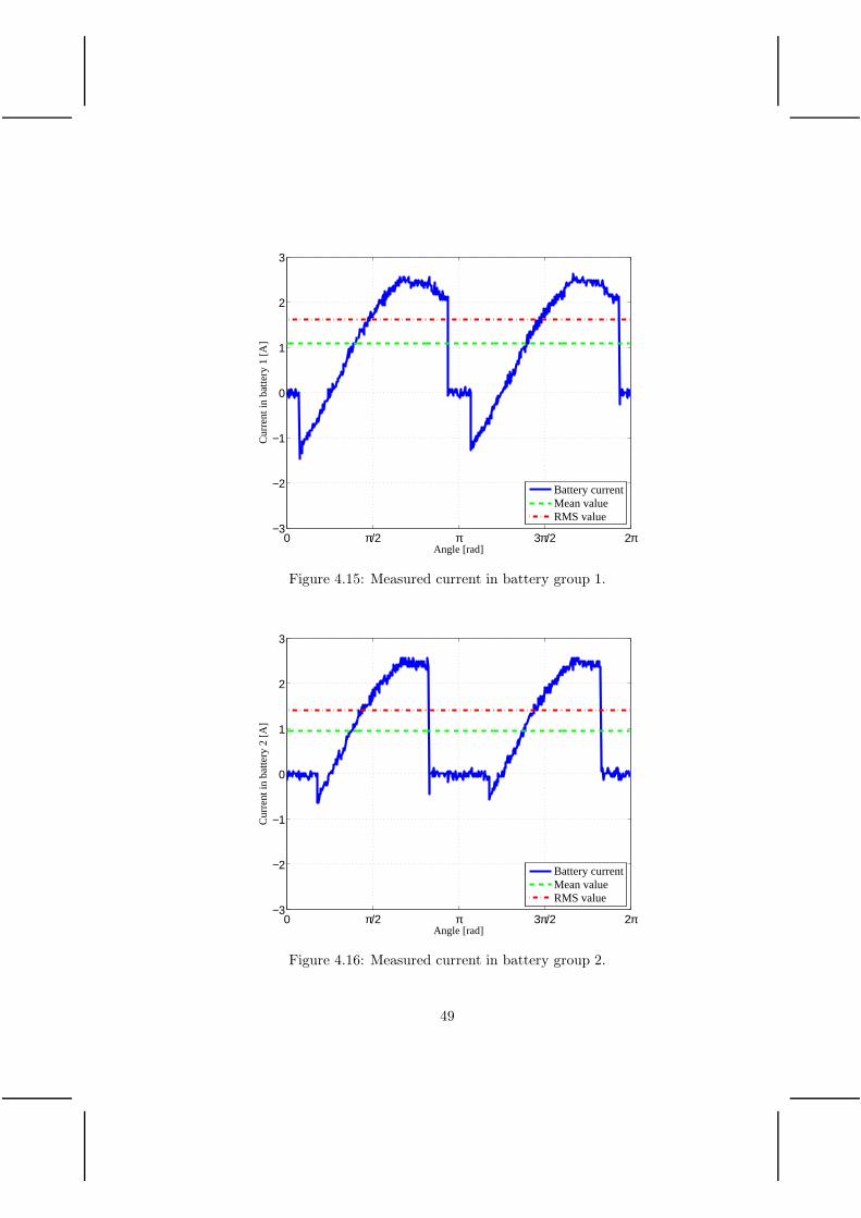
0 π/2 π 3π/2 2π−3
−2
−1
0
1
2
3
Angle [rad]
Cur
rent
in b
atte
ry 1
[A]
Battery currentMean valueRMS value
Figure 4.15: Measured current in battery group 1.
0 π/2 π 3π/2 2π−3
−2
−1
0
1
2
3
Angle [rad]
Cur
rent
in b
atte
ry 2
[A]
Battery currentMean valueRMS value
Figure 4.16: Measured current in battery group 2.
49
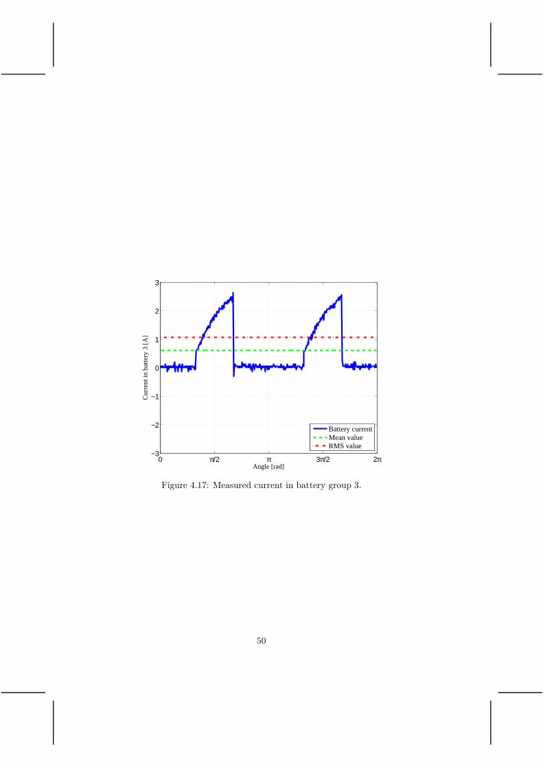
0 π/2 π 3π/2 2π−3
−2
−1
0
1
2
3
Angle [rad]
Cur
rent
in b
atte
ry 3
[A]
Battery currentMean valueRMS value
Figure 4.17: Measured current in battery group 3.
50

Chapter 5
Small PEV power train loss
evaluation
5.1 Efficiency calculations
When an inverter is used to supply the electric machine in an electric vehicle,the losses of the inverter are dependant on the operating points of the car.Based on the operating points given in Fig. 4.1 to 4.3, the losses in theinverter and in the battery are calculated according to Chapter 3 for therespective systems.
The analysis will mainly be done using the 50 km PEV while at end,results for a 200 km EV will also be presented.
5.1.1 Inverter
The losses in the two different inverters are calculated assuming that thecurrent to the electrical machine is equal for the two cases and that theharmonic levels are low and can accordingly be ignored in the loss calculationsfor the inverters.
Two level inverter
The power loss for the TLI using IGBTs is calculated for different torquesand speeds and is shown in Fig. 5.1 for a switching frequency of 10 kHzusing (3.25). It can be seen that the losses increase quite proportionally tothe current and so does also the torque. The losses are not speed dependentsince the magnetic losses in the the machine are neglected. However, when
51
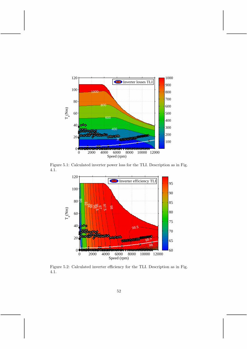
Speed (rpm)
Te(N
m)
1000
800
600
400
200
0 2000 4000 6000 8000 10000 120000
20
40
60
80
100
120
100
200
300
400
500
600
700
800
900
1000Inverter losses TLI
Figure 5.1: Calculated inverter power loss for the TLI. Description as in Fig.4.1.
Speed (rpm)
Te(N
m)
80 92 94 95 9696.597
97.5
98
98.5
98.5
98
0 2000 4000 6000 8000 10000 120000
20
40
60
80
100
120
60
65
70
75
80
85
90
95Inverter efficiency TLI
Figure 5.2: Calculated inverter efficiency for the TLI. Description as in Fig.4.1.
52

the field weakening region in entered, a current to demagnetize the machineis needed which increase the losses at higher speeds.
The efficiency of the inverter is shown in Fig. 5.2. Since the losses andthe output power both increase proportionally to the torque, the efficiency ofthe inverter is not particulary dependant of the torque. Since the losses arenot dependant on the speed but the output power is, it can be seen that theefficiency increases with speed. At high speeds and low torques the outputpower is low but the inverter has relatively high losses. These losses are dueto that the inverter needs to supply a current to demagnetise the machine inthe field weakening region (i.e. reactive current), and the inverter efficiencytherefore drops at high speeds.
Multilevel inverter
The inverter losses with the MLI at different speeds and torques producedby the electrical machine can be seen in Fig. 5.5 for the MLI presented inTable 4.3. The conductive loss, using (3.19) and (3.20), and the switch loss,using (3.23) and (3.24), can be seen in Fig. 5.3 and Fig. 5.4. It can benoted that the conductive loss in the MOSFETs totally dominates the lossessince the inverter is only switched at the fundamental frequency. Even at themaximum speed, the switching losses never exceeds 15 W for the inverter.Since the conductive loss in a MOSFET is proportional to the square of thecurrent, the loss increases with the square of the torque in the region withoutfield weakening. In the field weakening region the losses increase for a certaintorque as the speed increases, since extra current is needed to demagnetizethe machine.
The efficiency of the MLI can be seen in Fig. 5.6. Since the power loss isproportional to the square of the torque and the output power is proportionalto the torque, this means that at a certain speed the efficiency drops for highertorques. When increasing the speed, the output power increases and the lossremains fairly constant for a certain torque. This causes the efficiency toincrease at higher speeds. When entering the field weakening region, theefficiency drops since more current is needed to demagnetize the machine.
53

Speed (rpm)
Te(N
m)
200
100
50
25
0 2000 4000 6000 8000 10000 120000
20
40
60
80
100
120
0
200
400
600
800
1000Inverter conduction loss MLI
Figure 5.3: Calculated inverter conduction loss for the MLI. Description asin Fig. 4.1.
Speed (rpm)
Te(N
m)
1
2
5
10
0 2000 4000 6000 8000 10000 120000
20
40
60
80
100
120
0
200
400
600
800
1000Inverter switch loss MLI
Figure 5.4: Calculated inverter switch loss for the MLI. Description as in Fig.4.1.
54

Speed (rpm)
Te(N
m)
200
100
50
25
0 2000 4000 6000 8000 10000 120000
20
40
60
80
100
120
0
200
400
600
800
1000Inverter losses MLI
Figure 5.5: Calculated inverter power loss for the MLI. Description as in Fig.4.1.
Speed (rpm)
Te(N
m)
9797
.598
.599
99.5
0 2000 4000 6000 8000 10000 120000
20
40
60
80
100
120
50
60
70
80
90
100Inverter efficiency MLI
Figure 5.6: Calculated inverter efficiency for the MLI. Description as in Fig.4.1.
55

5.1.2 Battery
The battery loss for the car when using a TLI is shown in Fig. 5.7 forthe battery presented in Section 4.1.2. Since the whole battery supplies thepower to the electric machine and the voltage in the battery is assumed tobe constant, the battery current becomes proportional to the active powersupplied to the machine. The losses in the battery then become proportionalto the square of the electric machine power. This can be seen in Fig. 5.7for all operation points. Due to that the TLI balances the reactive power inthe separate phases already in the inverter and also smoothens a very highfrequency ripple with its DC-link capacitor, the battery utilization becomesas good as it can be with the TLI. When switching to a MLI the question is,how much extra losses will be added.
Speed (rpm)
Te(N
m)
250
500
1000
2000
0 2000 4000 6000 8000 10000 120000
20
40
60
80
100
120
0
1000
2000
3000
4000
5000
6000Battery losses TLI
Figure 5.7: Calculated losses in the battery when using a TLI. Descriptionas in Fig. 4.1.
In this chapter, two battery loss investigation will be performed. Onewith no filter capacitors over the battery groups and on with an extremelylarge capacitor. This is done in order to provide the complete loss range thatthe battery in the MLI can be exposed to. In Chapter 7 a more throughinvestigation of the capacitor influence will be performed where a variationof capacitor sizes and chemistries will be used.
The battery losses when operating the vehicle with infinity large capaci-tors to the input of a MLI can be seen in Fig. 5.8. The battery loss will be
56
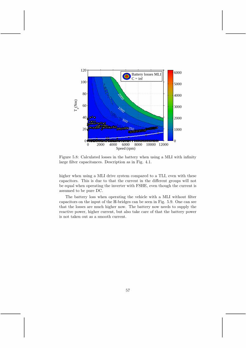
Speed (rpm)
Te(N
m)
250
500
1000
2000
0 2000 4000 6000 8000 10000 120000
20
40
60
80
100
120
0
1000
2000
3000
4000
5000
6000Battery losses MLIC = inf
Figure 5.8: Calculated losses in the battery when using a MLI with infinitylarge filter capacitances. Description as in Fig. 4.1.
higher when using a MLI drive system compared to a TLI, even with thesecapacitors. This is due to that the current in the different groups will notbe equal when operating the inverter with FSHE, even though the current isassumed to be pure DC.
The battery loss when operating the vehicle with a MLI without filtercapacitors on the input of the H-bridges can be seen in Fig. 5.9. One can seethat the losses are much higher now. The battery now needs to supply thereactive power, higher current, but also take care of that the battery poweris not taken out as a smooth current.
57

Speed (rpm)
Te(N
m)
250
500
1000
2000
3000
4000
5000
0 2000 4000 6000 8000 10000 120000
20
40
60
80
100
120
0
1000
2000
3000
4000
5000
6000Battery losses MLIC = 0
Figure 5.9: Calculated losses in the battery when using a MLI without filtercapacitances. Description as in Fig. 4.1.
58

5.1.3 Combined inverter and battery losses
The total inverter-battery losses that are analysed and presented below, con-sist of the inverter losses and the battery losses. The machine losses areassumed to be equal for the two inverters and are therefore excluded in thisanalysis.
For the TLI, the total losses of the battery and the inverter are shown inFig. 5.10.
Speed (rpm)
Te(N
m)
250
500
1000
2000
3000
0 2000 4000 6000 8000 10000 120000
20
40
60
80
100
120
0
1000
2000
3000
4000
5000
6000Total losses TLI
Figure 5.10: Calculated inverter and battery losses for the TLI. Descriptionas in Fig. 4.1.
For the MLI with large capacitors in parallel to the input of the H-bridges,the losses are shown in Fig. 5.11, and for the MLI without input capacitorsthe losses are shown in Fig. 5.12. The drive system with the MLI with largecapacitors shows an advantage over the TLI drive system at all operatingpoints. For the MLI system without capacitors, as expected, the losses be-come larger than for the TLI systems at high speeds and high output power.Only at the lowest speed range there is a benefit for the MLI system alsofor high torques. In order to evaluate the accumulated loss picture, drivecycle analysis must be performed. The result of such a study is presented inSection 5.2.
59

Speed (rpm)
Te(N
m)
250
500
1000
2000
0 2000 4000 6000 8000 10000 120000
20
40
60
80
100
120
0
1000
2000
3000
4000
5000
6000Total losses MLIC = inf
Figure 5.11: Calculated inverter and battery losses for the MLI with capaci-tors. Description as in Fig. 4.1.
Speed (rpm)
Te(N
m)
250
500
1000
2000
3000
40005000
6000
0 2000 4000 6000 8000 10000 120000
20
40
60
80
100
120
0
1000
2000
3000
4000
5000
6000Total losses MLIC = 0
Figure 5.12: Calculated inverter and battery losses for the MLI without ca-pacitors. Description as in Fig. 4.1.
60

5.1.4 Loss comparison
In the 2D-contours in the previous section, it was not easy to make a compar-ison between the loss maps. Therefore the loss comparison will be performedusing graphs for fixed torques instead.
The losses in the inverters for different speeds and a fixed torque of 10Nmare shown in Fig. 5.13, and for a torque of 60 Nm in Fig. 5.14. It can beseen that the MLI has lower inverter losses for all operating points. It canalso be noticed that the inverter losses for both the MLI and the TLI increasea lot when entering the field weakening region.
The losses in the battery for different speeds and a fixed torque of 10 Nmare shown in Fig. 5.15, and for a torque of 60 Nm in Fig. 5.16. The lossesin the battery for the TLI are lowest for all speeds. This is due to thatthe current out from the battery is a pure DC. The battery losses for theMLI with infinitely large capacitors to the inputs of the H-bridges are a bithigher. The batteries do not supply the uneven current from the reactivepower demand of the electric machine, but some of the battery modules havea higher current than other ones, even though they have a pure DC current.The losses for the MLI without capacitors are higher for all speeds, especiallywhen entering the field weakening region. The batteries must then supplythe waveforms to form the increased reactive power needed by the electricmachine at this region and this increases the losses due to a higher batterycurrent.
The total losses for the drive systems for different speeds and a fixedtorque of 10 Nm is shown in 5.17, and in Fig. 5.18 the total losses are shownfor a torque of 60 Nm. When operating the machine at low torques, thelosses for the MLI drive system are lower for low speeds. When enteringthe field weakening region the battery losses increase drastically for the MLIdrive system since the uneven waveforms needed to form the reactive powerneeded by the electric machine can not be supplied from the capacitors andinstead must come from the battery. For higher torques the TLI drive systemshows lower losses for almost all speeds, if one does not have the possibilityto filter out the reactive power and the harmonic content from the batteryin the MLI drive system. As mentioned before, the electric machine will onthe other hand not operate at this high torque very often which makes theenergy efficiency to be potentially higher for the MLI system. This calls fora complete drive cycle analysis.
61

0 2000 4000 6000 8000 10000 120000
50
100
150
200
250
300
Speed (rpm)
Pow
er lo
ss (
W)
Inverter loss with TLIInverter loss with MLI
Figure 5.13: Calculated inverter power loss for T=10 Nm.
0 2000 4000 6000 8000 10000 12000100
200
300
400
500
600
700
800
900
Speed (rpm)
Pow
er lo
ss (
W)
Inverter loss with TLIInverter loss with MLI
Figure 5.14: Calculated inverter power loss for T=60 Nm.
62
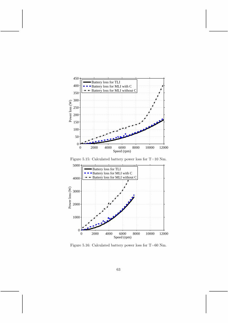
0 2000 4000 6000 8000 10000 120000
50
100
150
200
250
300
350
400
450
Speed (rpm)
Pow
er lo
ss (
W)
Battery loss for TLIBattery loss for MLI with CBattery loss for MLI without C
Figure 5.15: Calculated battery power loss for T=10 Nm.
0 2000 4000 6000 8000 10000 120000
1000
2000
3000
4000
5000
Speed (rpm)
Pow
er lo
ss (
W)
Battery loss for TLIBattery loss for MLI with CBattery loss for MLI without C
Figure 5.16: Calculated battery power loss for T=60 Nm.
63
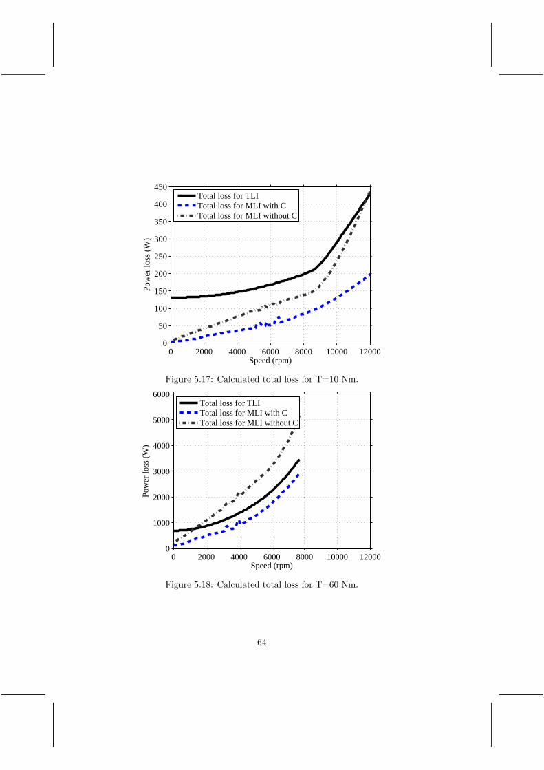
0 2000 4000 6000 8000 10000 120000
50
100
150
200
250
300
350
400
450
Speed (rpm)
Pow
er lo
ss (
W)
Total loss for TLITotal loss for MLI with CTotal loss for MLI without C
Figure 5.17: Calculated total loss for T=10 Nm.
0 2000 4000 6000 8000 10000 120000
1000
2000
3000
4000
5000
6000
Speed (rpm)
Pow
er lo
ss (
W)
Total loss for TLITotal loss for MLI with CTotal loss for MLI without C
Figure 5.18: Calculated total loss for T=60 Nm.
64
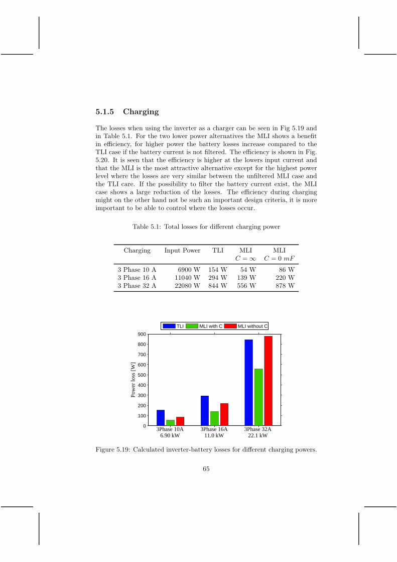
5.1.5 Charging
The losses when using the inverter as a charger can be seen in Fig 5.19 andin Table 5.1. For the two lower power alternatives the MLI shows a benefitin efficiency, for higher power the battery losses increase compared to theTLI case if the battery current is not filtered. The efficiency is shown in Fig.5.20. It is seen that the efficiency is higher at the lowers input current andthat the MLI is the most attractive alternative except for the highest powerlevel where the losses are very similar between the unfiltered MLI case andthe TLI care. If the possibility to filter the battery current exist, the MLIcase shows a large reduction of the losses. The efficiency during chargingmight on the other hand not be such an important design criteria, it is moreimportant to be able to control where the losses occur.
Table 5.1: Total losses for different charging power
Charging Input Power TLI MLI MLIC = ∞ C = 0 mF
3 Phase 10 A 6900 W 154 W 54 W 86 W3 Phase 16 A 11040 W 294 W 139 W 220 W3 Phase 32 A 22080 W 844 W 556 W 878 W
0
100
200
300
400
500
600
700
800
900
3Phase 10A6.90 kW
3Phase 16A11.0 kW
3Phase 32A22.1 kW
Pow
er lo
ss [W
]
TLI MLI with C MLI without C
Figure 5.19: Calculated inverter-battery losses for different charging powers.
65

90
92
94
96
98
100
3Phase 10A6.90 kW
3Phase 16A11.0 kW
3Phase 32A22.1 kW
Effi
cien
cy [%
]
TLI MLI with C MLI without C
Figure 5.20: Calculated inverter-battery efficiency for different chargingpower
5.2 Drive cycle evaluation
The accumulated energy loss for the battery and the inverter are now ana-lyzed using the NEDC, the FTP75, the HWFET and the US06 drive cyclesfor the vehicle presented in Table 4.1.
5.2.1 NEDC
The torque and speed profile for the NEDC drive cycle are shown in Fig.5.21 and in Fig. 4.5.
The battery and inverter accumulated losses for the three different setupsare shown in Fig. 5.22. One can see that the accumulated losses for the TLIdrive system becomes the worst ending up at 43Wh. The MLI that does nothave capacitors to filter out the reactive power and harmonic content uses30Wh. This is an improvement over the TLI and as can be seen in Fig. 5.29,the inverter losses have been reduced substantially. The battery losses areincreased but the sum is reduced. When having a large enough capacitor tothe input of the H-bridges the reactive power supply is assumed to be takenfrom these capacitors instead of the battery. The losses in the battery arethen reduced to only 13 Wh instead of 27 Wh. The total losses are thenreduced to 16 Wh.
66

Speed (rpm)
Te(N
m)
0 2000 4000 6000 8000 10000 120000
20
40
60
80
100
120
Figure 5.21: Operation points of the electric machine during NEDC
0 200 400 600 800 1000 12000
5
10
15
20
25
30
35
40
45
Time (s)
Acc
umul
ated
loss
es (
Wh)
TLIMLI with CMLI without C
Figure 5.22: Losses during the NEDC drive cycle
67
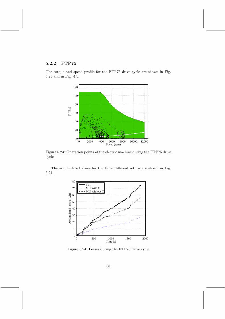
5.2.2 FTP75
The torque and speed profile for the FTP75 drive cycle are shown in Fig.5.23 and in Fig. 4.5.
Speed (rpm)
Te(N
m)
0 2000 4000 6000 8000 10000 120000
20
40
60
80
100
120
Figure 5.23: Operation points of the electric machine during the FTP75 drivecycle
The accumulated losses for the three different setups are shown in Fig.5.24.
0 500 1000 1500 20000
10
20
30
40
50
60
70
80
Time (s)
Acc
umul
ated
loss
es (
Wh)
TLIMLI with CMLI without C
Figure 5.24: Losses during the FTP75 drive cycle
68

5.2.3 HWFET
The torque and speed profile for the HWFET drive cycle are shown in Fig.5.25 and in Fig. 4.5.
Speed (rpm)
Te(N
m)
0 2000 4000 6000 8000 10000 120000
20
40
60
80
100
120
Figure 5.25: Operation points of the electric machine during the HWFETdrive cycle
The accumulated losses for the three different setups are shown in Fig.5.26.
0 200 400 600 8000
5
10
15
20
25
30
35
40
Time (s)
Acc
umul
ated
loss
es (
Wh)
TLIMLI with CMLI without C
Figure 5.26: Losses during the HWFET drive cycle
69

5.2.4 US06
The torque and speed profile for the US06 drive cycle are shown in Fig. 5.27and in Fig. 4.5.
Speed (rpm)
Te(N
m)
0 2000 4000 6000 8000 10000 120000
20
40
60
80
100
120
Figure 5.27: Operation points of the electric machine during the US06 drivecycle
The accumulated losses for the three different setups are shown in Fig.5.28.
0 100 200 300 400 500 6000
10
20
30
40
50
60
70
80
Time (s)
Acc
umul
ated
loss
es (
Wh)
TLIMLI with CMLI without C
Figure 5.28: Losses during the US06 drive cycle
70
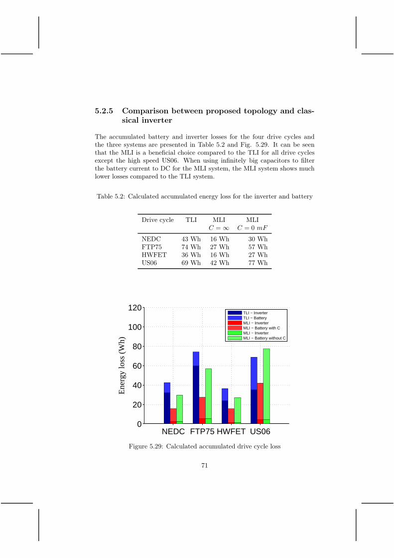
5.2.5 Comparison between proposed topology and clas-sical inverter
The accumulated battery and inverter losses for the four drive cycles andthe three systems are presented in Table 5.2 and Fig. 5.29. It can be seenthat the MLI is a beneficial choice compared to the TLI for all drive cyclesexcept the high speed US06. When using infinitely big capacitors to filterthe battery current to DC for the MLI system, the MLI system shows muchlower losses compared to the TLI system.
Table 5.2: Calculated accumulated energy loss for the inverter and battery
Drive cycle TLI MLI MLIC = ∞ C = 0 mF
NEDC 43 Wh 16 Wh 30 WhFTP75 74 Wh 27 Wh 57 WhHWFET 36 Wh 16 Wh 27 WhUS06 69 Wh 42 Wh 77 Wh
NEDC FTP75 HWFET US060
20
40
60
80
100
120
Ene
rgy
loss
(W
h)
TLI − InverterTLI − BatteryMLI − InverterMLI − Battery with CMLI − InverterMLI − Battery without C
Figure 5.29: Calculated accumulated drive cycle loss
71

5.3 40 kWh battery
A 40 kWh battery gives an approximate driving of 200 km, a suitable choicefor a pure electric vehicle. When increasing the battery size for the vehicle,the battery resistance is lowered. Therefore the battery losses compared to asmaller battery is lowered. In Fig. 5.30, the battery loss when using a 40 kWhbattery is shown. It can be noticed that the battery loss for all operatingpoints are lowered by a factor of 4 compared to the previously used 10 kWhbattery shown in Fig. 5.7.
Speed (rpm)
Te(N
m)
250
500
0 2000 4000 6000 8000 10000 120000
20
40
60
80
100
120
0
500
1000
1500Battery losses TLI
Figure 5.30: Calculated losses in the 40 kWh battery when using a TLI.Description as in Fig. 4.1.
The same energy content is also placed in the MLI setup giving a resultingloss map shown in Fig. 5.31. The losses for this setup is also lowered with afactor of 4 compared to the 10 kWh system shown in Fig. 5.9.
When operating the vehicle with the 40 kWh batteries in drive cycles, thebattery loss part of the accumulated loss is lowered by a factor of 4, see Fig.5.32. For the TLI system, this has a minor influence since the inverter losswas dominant already in the 10 kWh case. For the MLI case, the situation isthe opposite. In the 10 kWh case the battery loss was the dominant part ofthe accumulated loss during the drive cycles. By increasing the battery packto 40 kWh, the battery loss is lowered and thereby the accumulated drivecycles loss is very much reduced. It can be noted that the MLI setup is nowbeneficial from a loss perspective for all the analysed drive cycles.
72
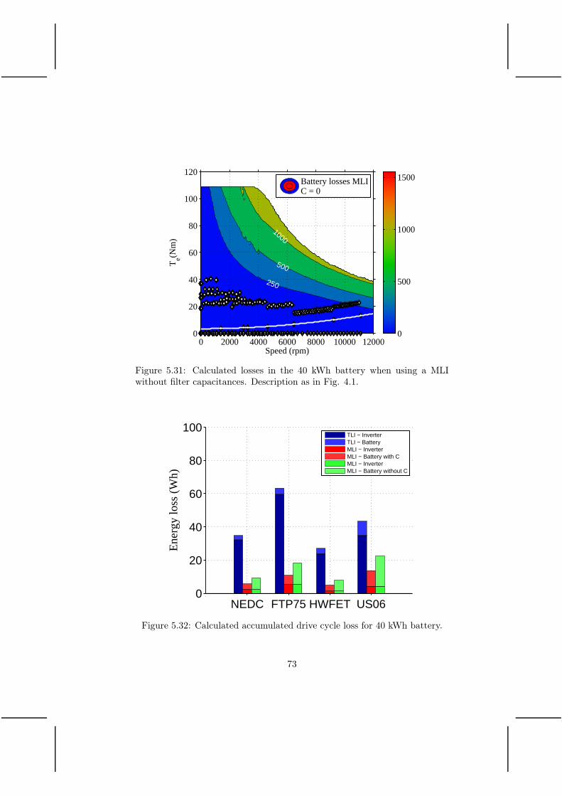
Speed (rpm)
Te(N
m)
250
500
1000
0 2000 4000 6000 8000 10000 120000
20
40
60
80
100
120
0
500
1000
1500Battery losses MLIC = 0
Figure 5.31: Calculated losses in the 40 kWh battery when using a MLIwithout filter capacitances. Description as in Fig. 4.1.
NEDC FTP75 HWFET US060
20
40
60
80
100
Ene
rgy
loss
(W
h)
TLI − InverterTLI − BatteryMLI − InverterMLI − Battery with CMLI − InverterMLI − Battery without C
Figure 5.32: Calculated accumulated drive cycle loss for 40 kWh battery.
73

5.4 Slim sizing of the inverter semiconductors
The selected IGBT for the previous analysis is the FS800 from Infineon.It has a maximum current of 800 A meaning about 400 A rms current asmaximum value. If instead the FS400 module is selected, the losses are notincreased much, see Fig. 5.33 compared to Fig. 5.1. The fixed voltage dropstill exists, the resistance is increased, but the switching losses are decreased abit. If the FS400 is used instead of the FS800 the losses in the TLI thereforeremains quite constant, however, this module can not dissipate the sameamount of power loss so a degradation of the performance might be neededduring specific conditions.
Speed (rpm)
Te(N
m)
1000
800
600
400
200
0 2000 4000 6000 8000 10000 120000
20
40
60
80
100
120
100
200
300
400
500
600
700
800
900
1000Inverter losses TLI
Figure 5.33: Calculated inverter power loss for the slim sized TLI. Descriptionas in Fig. 4.1.
The current rating of the IGBT module for the TLI system in Fig. 5.33 isreduced to half. To make a fair comparison the amount of semiconductors inthe MLI system is decreased to half, putting an equivalent of 2.5 MOSFETsin parallel for each switch position in the H-bridge. The equivalent resistancefor the MOSFETs are thereby doubled and since the switching losses for theMLI system are almost neglectable, the losses are quite simply doubled, seeFig. 5.34 compared to Fig. 5.5.
Operating the vehicle with the slim sized inverter in drive cycles, theaccumulated loss for the TLI system is marginally changed. For the MLIsystem, the inverter loss is about doubled but since the battery loss for this
74

Speed (rpm)
Te(N
m)
400
200
100
5025
0 2000 4000 6000 8000 10000 120000
20
40
60
80
100
120
0
200
400
600
800
1000
Inverter losses MLI
Figure 5.34: Calculated inverter power loss for the slim sized MLI. Descrip-tion as in Fig. 4.1.
system is dominant, it does not influence the accumulated loss very much.The MLI system is still the beneficial choice compared to the TLI system forall analysed drive cycles except the US06 drive cycle.
75

NEDC FTP75 HWFET US060
20
40
60
80
100
120
Ene
rgy
loss
(W
h)
TLI − InverterTLI − BatteryMLI − InverterMLI − Battery with CMLI − InverterMLI − Battery without C
Figure 5.35: Calculated accumulated drive cycle loss for the slim sized sys-tems.
76

Chapter 6
Battery loss modeling
To be able to calculate the battery loss and performance, a suitable model ofthe battery is needed. Since the multilevel inverter stresses the battery witha pulsed current which has a frequency of twice the fundamental electric ma-chine frequency, the models and parameters commonly used for simulationsof hybrid electric vehicles might not be suitable. In particular the method ofusing a pure resistance, which might be a function of SOC and temperature,as well as current direction. The battery cell is here modelled using the Ran-dles model, see [19], with three time constants and can be seen in Fig. 6.1.The model is chosen to include three time-constants to be able to cover allthe frequency domains that the battery is operated at. R0 to R3 and C1 toC3 describe the dynamic performance, and VOCV is the open circuit voltagewhich is dependant on the SOC. Since the frequency range is below a coupleof kHz, the battery inductance is assumed to be neglectable in the furtheranalysis.
Battery cell
R0
VOCV
R1
C1
+
VCell
-
R2
C2
R3
C3
Figure 6.1: The three time constants Randles model of the battery cell
77

6.1 Parameter extraction
Cell measurements are done on a ANR26650M1A cell from A123 systems fordifferent SOCs at a temperature of 25 C. A resistive load is connected tothe output of one H-bridge and one cell is used as input. The cell voltage andcurrent is measured with an oscilloscope. The H-bridge is then controlled tostress the battery cell with a pulsed current of different magnitudes (28 Aand 49 A) and various frequencies (1-100 Hz).
The three time constants Randles model shown in Fig. 6.1 has an impedancethat is mathematically described as
Zcell(s) =b3s
3 + b2s2 + b1s+ b0
s3 + a2s2 + a1s+ a0(6.1)
or with its corresponding poles, p3, p2 and p1, and zeros, z3, z2 and z1 as
Zcell(s) = b3(s− z3)(s− z2)(s− z1)
(s− p3)(s− p2)(s− p1). (6.2)
The corresponding electrical parameters can be calculated from the least-square fit impedance model knowing the transfer function and its correspond-ing poles. From the poles, the system time constants are calculated accordingto
τ3τ2τ1
= −
1/p31/p21/p1
. (6.3)
Knowing the time constants, a matrix A is created according to
A =1
τ1τ2τ3·
τ1τ2τ3 0 0 0τ1τ2 + τ1τ3 + τ2τ3 τ2τ3 τ1τ3 τ1τ2
τ1 + τ2 + τ3 τ2 + τ3 τ1 + τ3 τ1 + τ21 1 1 1
(6.4)
which can be used to calculate the resistances as
R3
R2
R1
R0
= A−1
b3b2b1b0
. (6.5)
The capacitances can now be calculated as
C3
C2
C1
=
τ3 0 00 τ2 00 0 τ1
1/R3
1/R2
1/R1
. (6.6)
78
If the Randles system instead is a two or one time-constant system, theleast-square system is calculated in a corresponding way.
The impendence is determined using a least-square fit on the measureddata and a part of one measurement can be seen in Fig. 6.2. Apart from the3p3z model, a 2p2z and a 1p1z as well as a resistive model is parameterised.It can be noted that the 2p2z, 1p1z and resistive model does not fit the highfrequency behaviour very well, but show a great match for lower frequencieswhere the pulsed waveform goes towards steady state. However, the 3p3z fitshows a great fit for the whole curve with a normalized root mean squaredeviation of 99.49 %.
The resulting Bode plot for the least-square curve fits for the 3p3z modelfor different measurements are shown in Fig. 6.3. First, it can be noted thatthe magnitude fit is excellent when using the model with three poles andthree zeros. Moreover it can be observed that the impedance becomes a bithigher at higher currents when comparing the four measurements in Fig. 6.3.An EIS sweep has also been performed in the frequency range of 10 mHz to10 kHz using the network analyser "Gamry reference 3000".
The resulting parameters and normalized root mean square deviation ofthe curve fits can be seen in Table 6.1. For the further analysis the data set’meas 3.23V 1Hz 28A’ is chosen due to that it matches the measurements atboth low and high frequencies, see Fig. 6.2.
Moreover, it can be noted that a DC resistance of 15 mΩ much betterrepresents the battery cell compared to the 10mΩ specified in the data sheet.
6.2 Verification in experimental system
To verify the theory assumptions and to demonstrate the concept correctness,the small scale experimental system seen in Fig. 4.6 is utilised. The batterypack consists of 4 cells in series, connected to each H-bridge, which gives anominal voltage of 13.2 V for each H-bridge, and a total inverter capacity of270 Wh. This gives a scale in voltage as
VLargeScale = 3.8 · VSmallScale (6.7)
and a scale in current as
ILargeScale = 9.7 · ISmallScale. (6.8)
When four cells are connected into a battery pack, busbars and/or cablesare needed to connect the battery to the inverter. In order to account forthis additional resistance, a resistance Rcable is modeled in series with the
79
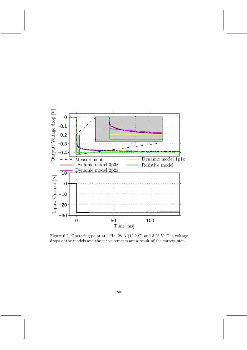
−0.4
−0.3
−0.2
−0.1
0
Output:
Voltage
drop[V]
0 50 100−30
−20
−10
0
10
Time [ms]
Input:
Current[A]
MeasurementDynamic model 3p3zDynamic model 2p2z
Dynamic model 1p1z
Resistive model
Figure 6.2: Operating point at 1 Hz, 28 A (12.2 C) and 3.23 V. The voltagedrops of the models and the measurements are a result of the current step.
80
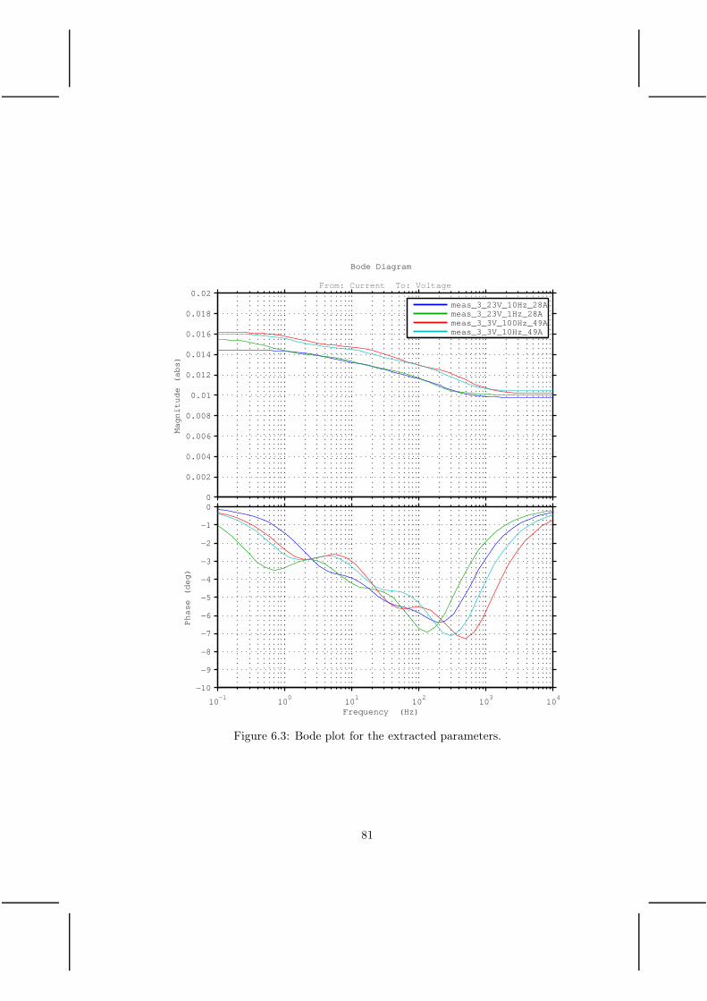
0
0.002
0.004
0.006
0.008
0.01
0.012
0.014
0.016
0.018
0.02From: Current To: Voltage
Ma
gn
itud
e (
ab
s)
10−1
100
101
102
103
104
−10
−9
−8
−7
−6
−5
−4
−3
−2
−1
0
Ph
ase
(d
eg
)
Bode Diagram
Frequency (Hz)
meas_3_23V_10Hz_28Ameas_3_23V_1Hz_28Ameas_3_3V_100Hz_49Ameas_3_3V_10Hz_49A
Figure 6.3: Bode plot for the extracted parameters.
81
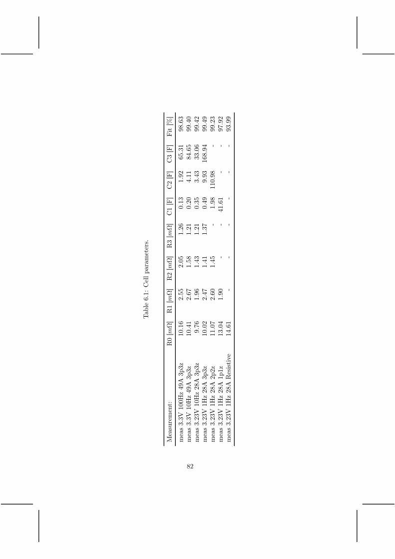
Tab
le6.
1:C
ellpa
ram
eter
s.
Mea
sure
men
t:R
0[m
Ω]
R1
[mΩ
]R
2[m
Ω]
R3
[mΩ
]C
1[F
]C
2[F
]C
3[F
]Fit
[%]
mea
s3.
3V10
0Hz
49A
3p3z
10.1
62.
552.
051.
260.
131.
9265
.31
98.6
3m
eas
3.3V
10H
z49
A3p
3z10
.41
2.67
1.58
1.21
0.20
4.11
84.6
599
.40
mea
s3.
23V
10H
z28
A3p
3z9.
761.
961.
431.
210.
353.
4333
.06
99.4
2m
eas
3.23
V1H
z28
A3p
3z10
.02
2.47
1.41
1.37
0.49
9.93
168.
9499
.49
mea
s3.
23V
1Hz
28A
2p2z
11.0
72.
601.
45-
1.98
110.
98-
99.2
3m
eas
3.23
V1H
z28
A1p
1z13
.04
1.90
--
41.6
1-
-97
.92
mea
s3.
23V
1Hz
28A
Res
istive
14.6
1-
--
--
-93
.99
82

Cable H-b
Iinput
Battery cell
+
V
-
Br ell
Br ell
Br ell
+
VD
-
Rc
Figure 6.4: Model of a battery pack, the cable and the optional input filterfor the small scale system.
battery pack and was measured to 9.17 mΩ. The system, when connected tothe multilevel inverter, can be seen in Fig. 6.4.
It should be noted that the battery cable resistance is unreasonable highin the small scale system. In the full scale system it is scaled according to thebattery cells and becomes lower, unfortunately not as low as a commercialvehicle would have.
6.2.1 Representative operating points for the full scalesystem
A vehicle operates in a wide range of speeds and torques, resulting in a widespeed-torque region for the electric drive system [53]. In order to cover therepresentative operating range of an electrified vehicle, detailed analysis ofthe battery performance was performed at six representative points takenfrom Fig. 4.1. The corresponding 6 inverter operating points for the smallpersonal vehicle presented in Table 4.1 with the PMSM machine presentedin Table 4.2 are shown in Table 6.2.
Table 6.2: Analysed operating points for the test vehicle system.
Case nr: n T Irms Uphase ϕ f
1 1000 RPM 30 Nm 78 Arms 17 Vrms 25 deg 83 Hz2 1000 RPM 60 Nm 137 Arms 22 Vrms 36 deg 83 Hz3 1000 RPM 90 Nm 185 Arms 28 Vrms 42 deg 83 Hz4 5000 RPM 30 Nm 78 Arms 77 Vrms 27 deg 417 Hz5 5000 RPM 60 Nm 137 Arms 103 Vrms 40 deg 417 Hz6 10000 RPM 30 Nm 101 Arms 106 Vrms 1 deg 833 Hz
83

To get the same operating points for the small scale system the operatingpoints are translated according to (6.7) and (6.8) and these are shown inTable 6.3.
Table 6.3: Analysed operating points for the experimental lab setup.
Case nr: n T Irms Uphase ϕ f
1 1000 RPM 30 Nm 8 Arms 4 Vrms 25 deg 83 Hz2 1000 RPM 60 Nm 14 Arms 6 Vrms 36 deg 83 Hz3 1000 RPM 90 Nm 19 Arms 7 Vrms 42 deg 83 Hz4 5000 RPM 30 Nm 8 Arms 20 Vrms 27 deg 417 Hz5 5000 RPM 60 Nm 14 Arms 27 Vrms 40 deg 417 Hz6 10000 RPM 30 Nm 10 Arms 28 Vrms 1 deg 833 Hz
6.2.2 Battery model performance in the MLI
The same measurement procedure is now made with the experimental inverter-battery MLI system for the six different operating points. The desired outputvoltage from Table 6.3 is recalculated to switching instances and an RL-loadis controlled to achieve the desired current and fundamental phase lag. InFig. 6.5, the battery current and voltage for case no 5 are shown for a smallperiod of time where both the measurement, the dynamic models and theresistive model are shown. It can thus be seen that the 3p3z dynamic modelfollows the measurement very well both for higher frequencies but also forthe lower ones. The 2p2z model agrees quite well with the measurementas well, and only overestimates the voltage drop with a few percents. The1p1z and the resistive model do however not agree well with the measure-ments and overestimate the voltage drop when a current is flowing in thecell (higher losses) and underestimates the voltage drop when no current isflowing through the cell. The resistive model is therefore only valid whena pure DC-current is flowing in the cells. However, this never occurs in amultilevel inverter drive system. Interesting to notice is that the EIS modelunderestimates the voltage drop and therefore the losses. The reason for thisis that the parameters are subtracted at a very low magnitude of current,and the battery impedance is in this case slightly lower at these low currentlevels.
The resulting losses for case no 5, as was displayed in Fig. 6.5, as well asthe other five cases are shown in Fig. 6.6 and the relative maximum voltagedrop compared to the measurements can be seen in Table 6.4. It can benoted that the dynamic model and the measurements agree very well and
84

−1
−0.5
0O
utpu
t: V
olta
ge d
rop
[V]
0 0.2 0.4 0.6 0.8 1 1.2 1.4 1.6
−15
−10
−5
0
Time [ms]
Inpu
t: C
urre
nt [A
]
MeasurementDynamic model 3p3zDynamic model 2p2z
Dynamic model 1p1zResistive modelEIS model
Figure 6.5: Battery current for operation point five when no input capacitoris used.
that the resistive model always overestimates the losses and the EIS modelunderestimates the losses. It can also be noted that the resistive model showssomewhat better agreement at lower frequencies (operating point one, twoand three) compared to higher frequencies (operating point six).
85

Table 6.4: Maximum voltage drop for the six operating points relative to themeasurement.
Case nr: 1 2 3 4 5 6
Measurement 100 % 100 % 100 % 100 % 100 % 100 %3p3z 98 % 101 % 98 % 101 % 100 % 102 %2p2z 98 % 101 % 101 % 105 % 104 % 108 %1p1z 107 % 111 % 112 % 119 % 118 % 123 %
Resistive 118 % 122 % 124 % 131 % 130 % 136 %EIS 91 % 94 % 91 % 94 % 93 % 95 %
1 2 3 4 5 60
2
4
6
8
10
12
Battery
pow
erloss
[W]
Operating point
95.3
%129.2
%
98.4
% 130.2
%
99.6
%132.2
%
100.0
%132.3
%
100.8
%146.5
%
100.4
%139.6
%
MeasurementModelResistive model
Figure 6.6: Calculated loss comparison between measurements, the dynamicmodel and a purely resistive model.
6.3 Drive cycle evaluation for battery losses
The five different battery models are now used in a drive cycle evaluation.The reference vehicle is used to calculate the operating points for the inverterfor the NEDC cycle. The resulting total battery loss can be seen in Fig. 6.7
86

NEDC FTP75 US06 HWFET0
10
20
30
40
50
60
70
80
90
100
110
Ene
rgy
stor
age
loss
for
the
who
le b
atte
ry [W
h]
Drive cycle
Dynamic model with 3 poles and 3 zerosDynamic model with 2 poles and 2 zerosDynamic model with 1 pole and 1 zeroResistive modelEIS model
Figure 6.7: Calculated loss comparison between the models for different drivecycles.
together with the three other investigated drive cycles. It can be noted thatthe same behaviour is shown for all the drive cycles even though the caroperates at very different speeds and accelerations in the four drive cycles.In the same way as for the single operating point verification, the resistivemodel shows a higher loss compared to the 3p3z dynamic model and the EISmodel provides a lower loss prediction.
87

88

Chapter 7
Filter capacitor influence
As described in Section 4.1.3, capacitors can be put over the battery groupsin order to alleviate the battery cells to some extent from ripply currents. InChapter 5 two "end-point options" were tested but here a more through anal-ysis of the capacitor influence is performed where various amounts are anal-ysed. The impact will also be analysed for two different capacitor chemistriesand the loss effect will be quantified.
7.1 System overview
To be able to analyse the impact of capacitors connected to the input of theH-bridges in a multilevel inverter, the experimental system is utilised whereit is possible to connect various combinations of capacitors to the inputs.It should be mentioned that there are always capacitors located over theH-bridges in the experimental system to supply and absorb energy duringthe switching instances in order to avoid voltage spikes on the transistorsHowever, here the amount is increased above what is needed for the circuit tooperate properly. Actually, since the switching instances occur very seldom,it is possible to switch more slowly and then these small capacitors are notneeded. The further analysis is performed at 25 C.
7.1.1 Battery cell
The battery cell is modeled with the three time-constant Randles model pre-sented in Fig. 6.1. The parameters used are derived through measurementsand are presented under model "meas 3.23V 1Hz 28A 3p3z" in Table 6.1 butcan also be seen below in Table 7.1.
89

For the full scale system the battery is described in Table 7.2 for eachH-bridge to get an understanding of the physical dimensions of the system.
90

Tab
le7.
1:C
ellpa
ram
eter
s.
Mea
sure
men
t:R
0[m
Ω]
R1
[mΩ
]R
2[m
Ω]
R3
[mΩ
]C
1[F
]C
2[F
]C
3[F
]Fit
[%]
3.23
V1H
z28
A10
.02
2.47
1.41
1.37
0.49
9.93
168.
9499
.49
Tab
le7.
2:B
atte
ryco
nfigu
ration
.Val
ues
per
H-b
ridg
e.
Nr
ofce
llsin
seri
esN
rof
cells
inpa
ralle
lD
C-r
esis
tanc
e[m
Ω]
Wei
ght
[kg]
Vol
ume
[L]
1510
22.9
12.5
5.28
91

7.2 Capacitor configurations
Eight configurations of capacitances are selected together with one configu-ration without any input capacitances. Four of the configurations are basedon a super capacitor chemistry and four configurations are based on an elec-trolytic chemistry. The parameters for configuration 1-8 and the case withoutany capacitances (configuration 0), are shown in Table 7.3. For verificationpurposes, configuration 0, configuration 4 and configuration 8 are scaled downto fit the experimental system. It should be noted that the electrolytic config-uration (configuration 1-4) has about the same mass and volume as the supercapacitance configuration (configuration 5-8). Accordingly, the capacitanceis a consequence of this selection.
92

Tab
le7.
3:C
apac
itor
confi
gura
tion
s,va
lues
per
H-b
ridg
e.
Con
figur
atio
n:C
olor
:So
rt:
Cap
acitan
ce[m
F]
Res
ista
nce
[mΩ
]W
eigh
t[k
g]Vol
ume
[L]
0N
/A-
--
-1
Ele
ctro
lytic
capa
cito
r5.
8752
.50.
550.
372
Ele
ctro
lytic
capa
cito
r23
.513
.12.
21.
53
Ele
ctro
lytic
capa
cito
r41
.17.
53.
92.
64
Ele
ctro
lytic
capa
cito
r58
.75.
255.
53.
75
Super
capa
cito
r44
4010
40.
460.
366
Super
capa
cito
r17
800
25.9
1.8
1.4
7Su
per
capa
cito
r31
100
14.8
3.2
2.5
8Su
per
capa
cito
r44
400
10.4
4.6
3.6
0 SS
(Sm
allSc
ale)
N/A
--
--
4 SS
(Sm
allSc
ale)
Ele
ctro
lytic
capa
cito
r22
140.
140.
098
8 SS
(Sm
allSc
ale)
Super
capa
cito
r16
700
27.6
0.12
0.09
4
93

7.3 Model verification
As in the previous chapter, the six operating points presented in Table 6.3are used to perform measurements in the small scale system and the configu-rations 0, 4 and 8 are scaled down and called configuration 0SS, 4SS and 8SS ,see Table 7.3 (SS stands for small scale). The voltage drop and current aresampled to be able to calculate the losses. The current is also used as inputto the models to calculate a simulated loss. These waveforms are presentedfor operating point 1 in Fig. 7.1.
−0.8
−0.6
−0.4
−0.2
0
Out
put:
Vol
tage
dro
p [V
]
0.5 1 1.5 2 2.5 3
−15
−10
−5
0
Time [ms]
Inpu
t: C
urre
nt [A
]
Config. 8ss measurementConfig. 0ss measurementConfig. 4ss measurement
Config. 8ss modelConfig. 0ss modelConfig. 4ss model
Figure 7.1: Simulations and measurements of the models in the small scalesystem for operating point 1.
It can be noted that the waveforms agree very well between the simula-tions and the measurements for each configuration. Almost the same currentwas used for the three measurements but as can be noticed in Fig. 7.1, thereare some small variations so a loss comparison between the setups could notbe specifically obtained by studying the figure even though the behaviourof the setups are very clearly illustrated. However, from the voltage-currentrelations the models could be verified individually.
94

The highest voltage drop is observed without the capacitances (configu-ration 0SS) while the electrolytic capacitance (configuration 4SS) holds thevoltage very good in the beginning of the pulse due to their low resistance.Since the electrolytic capacitor does not have a very high capacitance, thevoltage drop starts to increase quite quickly at the low frequency that op-erating point 1 has. The super capacitor configuration (8SS) shows a bitdifferent behaviour since it has higher resistance but more capacitance. Itshows a higher voltage drop in the beginning of the pulse compared to theelectrolytic configuration but holds this voltage drop since the capacitance isvery high.
The losses are calculated for all six operating points with all three con-figurations and compared with its measurements and presented in Table 7.4.Since the calculated losses agree within a few percents of the measurements,the models are concluded to be valid. Therefore the models will be used infurther calculations of the losses during different drive cycles.
Table 7.4: Loss comparison between models and measurements for six oper-ating points.
Configuration Op1 Op2 Op3 Op4 Op5 Op6
0SS 98.9 % 100.8 % 100.2 % 102.4 % 102.0 % 103.8 %4SS 100.4 % 99.4 % 99.7 % 101.5 % 102.2 % 102.8 %8SS 102.5 % 99.6 % 99.9 % 100.5 % 99.7 % 100.2 %
7.4 Frequency analysis
Operating point 1 and 6 are now selected for a more detailed harmonic anal-ysis and simulations are performed for several configurations. In Fig. 7.2 theharmonic spectrum of the battery pack voltage and current are shown forconfiguration 0 (pure battery) and configuration 4 (big electrolytic capaci-tor) at operating point 1. It should be noted that the capacitors suppress theharmonic content in the battery to a very large extent, lowering the secondharmonic with a factor of around 4 for both the voltage and current.
In Table 7.5, the harmonic content of the second, forth and highest har-monic above 9 kHz are shown. The 9 kHz frequency is chosen as the lowerlimit due to that some EMI requirement reach down to this frequency [54].For operating point 1 the super capacitors show the biggest improvementof the harmonic content due to the low frequency at operating point 1. At
95

0 2000 4000 6000 8000 10000 120000
0.2
0.4
0.6
0.8
Frequency [Hz]
|Vbatt|[V
]
0 2000 4000 6000 8000 10000 120000
10
20
30
40
Frequency [Hz]
|Ibatt|[A
]
(a) Configuration 0
0 2000 4000 6000 8000 10000 120000
0.2
0.4
0.6
0.8
Frequency [Hz]
|Vbatt|[V
]
0 2000 4000 6000 8000 10000 120000
10
20
30
40
Frequency [Hz]
|Ibatt|[A
]
(b) Configuration 4
Figure 7.2: Harmonic spectrum of the battery waveforms for operating point1. Units in amplitude
96

operating point 6 the frequency is much higher, therefore the electrolyticcapacitors show the best performance at operating point 6.
From an EMI perspective, it is important to minimize the voltage swings/ripplein the DC cables and all ’conducting surfaces’, since these are the sources forradiated emissions. The maximum amplitude at frequencies above 9 kHz isreduced significantly for both chemistries of capacitors at operating point 1,leading to an improved EMI situation. For operating point 6, the electrolyticcapacitors show the best improvement.
Table 7.5: Calculated harmonic content of the battery pack voltage for vari-ous filter capacitor configurations.
OP Config. 2nd harmonic 4th harmonic Highest above 9 kHz
OP1
0 866 mV 586 mV 17 mV1 827 mV 529 mV 13 mV4 480 mV 223 mV 4 mV5 729 mV 505 mV 15 mV8 297 mV 211 mV 6 mV
Mix 1 and 5 776 mV 518 mV 14 mVMix 4 and 8 389 mV 229 mV 5 mV
OP6
0 1179 mV 274 mV 30 mV1 634 mV 209 mV 23 mV4 194 mV 63 mV 7 mV5 714 mV 238 mV 27 mV8 302 mV 101 mV 11 mV
Mix 1 and 5 672 mV 222 mV 25 mVMix 4 and 8 238 mV 78 mV 9 mV
In Table 7.6, the second, forth and sixth harmonic for the battery cur-rent are shown. Here it can be noted that there is a clear reduction of thecurrent pulses stressing the battery with configuration 1-8 compared to con-figuration 0. For the low speed operating point 1, the second harmonic isfiltered best with the super capacitors due to its low frequency. the forthand sixth harmonic are lowered with around the same amount for the twocapacitor chemistries. At operating point 6, the electrolytic capacitors showa much better improvement for all harmonics due to the higher frequency atthis operating point.
97

Table 7.6: Calculated harmonic content of the battery pack current for vari-ous filter capacitor combinations.
OP Config. 2nd harmonic 4th harmonic 6th harmonic
OP1
0 43 A 31 A 16 A1 41 A 28 A 13 A4 24 A 12 A 5 A5 36 A 27 A 13 A8 15 A 11 A 6 A
Mix 1 and 5 39 A 27 A 13 AMix 4 and 8 19 A 12 A 5 A
OP6
0 45 A 15 A 6 A1 34 A 11 A 4 A4 10 A 3 A 1 A5 39 A 13 A 5 A8 16 A 5 A 2 A
Mix 1 and 5 36 A 12 A 5 AMix 4 and 8 13 A 4 A 2 A
7.5 Drive cycle analysis
Configurations 1-8 from Table 7.3 and a mix between the chemistries arenow used in simulations of the four drive cycles NEDC, FTP75, US06 andHWFET to be able to compare the performance. The battery current, ca-pacitor current and voltage drop are shown in Fig. 7.3 to 7.5 for a small partof the drive cycle HWFET at t = 260 s for configuration 0, 4, 8 and a mixbetween 4 & 8. The weight and volume of configuration 4 and 8 are verysimilar (a bit more for the electrolytic case) but the relation between the re-sistance and the capacitance are very different between the two chemistries.From the figures it can be seen that the electrolytic capacitor (configuration4) has less resistance than the super capacitor (configuration 8) and holds thevoltage well in the first period of time after the current is applied. Howeverthe capacitance is much smaller in configuration 4 compared to configura-tion 8 and after some hundreds of microseconds the voltage has dropped toa level lower than the super capacitor. Depending on the operating speed(frequency) of the car, the two chemistries have different advantages.
The total loss accumulation for the drive cycles are presented in Fig. 7.6.It can be noted that a substantial decrease of the accumulated battery lossoccurs when placing capacitors to the input of the H-bridges of a multilevel
98
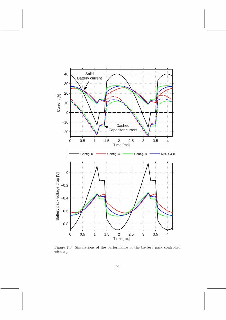
0 0.5 1 1.5 2 2.5 3 3.5 4
−0.8
−0.6
−0.4
−0.2
0
Bat
tery
pac
k vo
ltage
dro
p [V
]
Time [ms]
0 0.5 1 1.5 2 2.5 3 3.5 4
−20
−10
0
10
20
30
40
Cur
rent
[A]
Time [ms]
Config. 0 Config. 4 Config. 8 Mix. 4 & 8
SolidBattery current
DashedCapacitor current
Figure 7.3: Simulations of the performance of the battery pack controlledwith α1.
99

0 0.5 1 1.5 2 2.5 3 3.5 4
−0.8
−0.6
−0.4
−0.2
0
Bat
tery
pac
k vo
ltage
dro
p [V
]
Time [ms]
0 0.5 1 1.5 2 2.5 3 3.5 4
−20
−10
0
10
20
30
40
Cur
rent
[A]
Time [ms]
Config. 0 Config. 4 Config. 8 Mix. 4 & 8
SolidBattery current
DashedCapacitor current
Figure 7.4: Simulations of the performance of the battery pack controlledwith α2.
100

0 0.5 1 1.5 2 2.5 3 3.5 4
−0.8
−0.6
−0.4
−0.2
0
Bat
tery
pac
k vo
ltage
dro
p [V
]
Time [ms]
0 0.5 1 1.5 2 2.5 3 3.5 4
−20
−10
0
10
20
30
40
Cur
rent
[A]
Time [ms]
Config. 0 Config. 4 Config. 8 Mix. 4 & 8
SolidBattery current
DashedCapacitor current
Figure 7.5: Simulations of the performance of the battery pack controlledwith α3.
101

inverter used in electrified vehicles. The configurations with electrolytic ca-pacitors (configuration 1-4) show slightly lower accumulated loss comparedto the configurations with super capacitors (configurations 5-8) but they alsohave a bit higher mass.
With configurations 4 and 8 a reduction of the battery losses with around30 % is achieved. However, we have now added a mass of around 5 kg perH-bridge to a battery pack weighing 12.5 kg per H-bridge. In Fig. 7.7 the lossreduction as a function of added weight is plotted. It can be noted that addingcapacitors is always an advantage compared to adding more batteries for thefour drive cycles unless a large increase of the energy storage is conducted.For all of the four drive cycles it is an advantage from a loss perspective to adda certain mass of electrolytic capacitors instead of adding super capacitors.Adding a mix of the two chemistries show a similar effect where the lossesare at a level in between the super capacitor cases and the electrolytic cases.
If the mass of the capacitors were instead replaced with more batterycells, the losses in the battery would also be lowered, however, to a lowerextent unless a large increase is conducted.
To sum up, the most realistic case is with the lowest amount of capacitors.Since lifetime issues are not analysed and the EMI performance is only brieflyexamined, maybe even less capacitors than configuration 1 and 5 could bethe best choice.
7.6 Cold climate performance
For a cold battery it is of utmost important to avoid cyclings since the lifetime loss is substantial when the temperature goes to 0 deg C and belowaccording to [55]. At cold temperatures the battery increases its resistancevery much, an increase of approximately 400 % if the temperature drops from25C to 0C. The here used capacitors does not increase their resistance inthe same amount, roughly 20 % for the same temperature drop.
Operating point 1-6 are now simulated where the battery resistance isincreased 400 % and the capacitor resistance is increased 20%. The resultinglosses for configuration 0 (pure battery), 1 (small electrolytic capacitors)and 5 (small super capacitors) can be seen in Table 7.7. The loss reduction issignificantly improved even for these small capacitors, about 2.5 times greaterreduction for 0 deg C compared to 25 deg C. It can also be observed that theharmonic content is significantly reduced when adding these small capacitors.
102
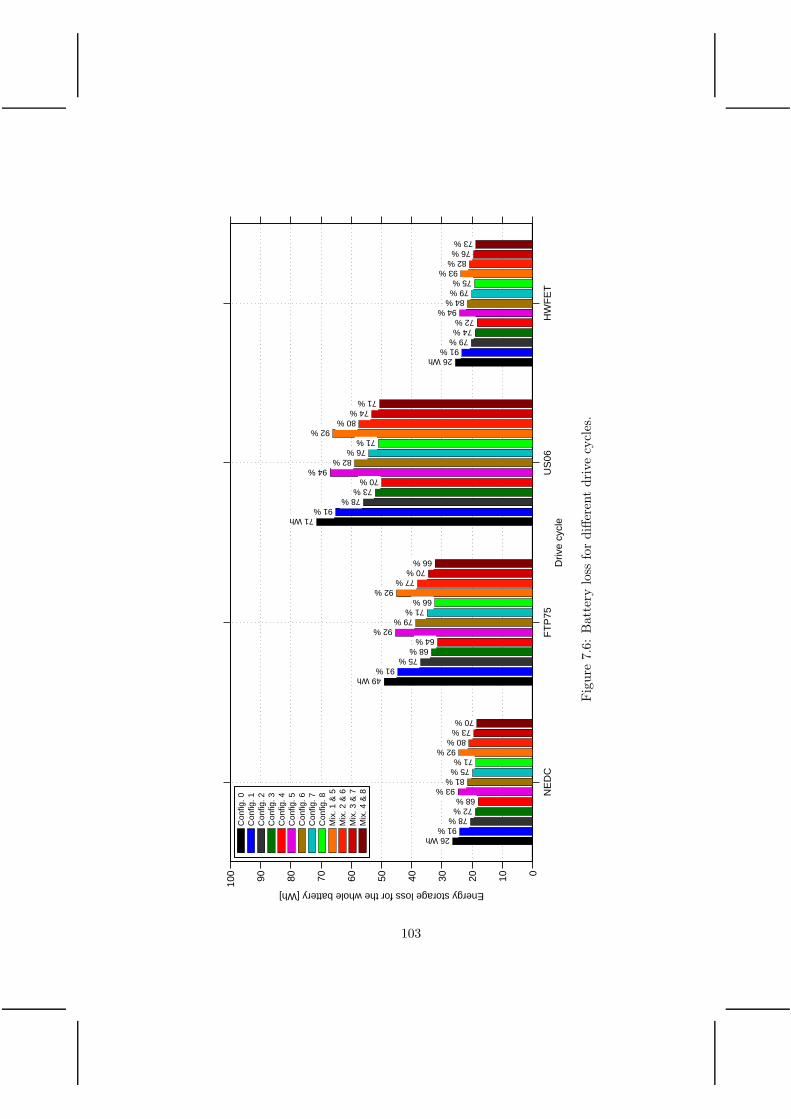
NE
DC
FT
P75
US
06H
WF
ET
0102030405060708090100
Energy storage loss for the whole battery [Wh]
Driv
e cy
cle
26 Wh91 %
78 %72 %
68 %93 %
81 %75 %
71 %92 %
80 %73 %
70 %
49 Wh91 %
75 %68 %
64 %92 %
79 %71 %
66 %92 %
77 %70 %
66 %
71 Wh91 %
78 %73 %
70 %94 %
82 %76 %
71 %92 %
80 %74 %
71 %
26 Wh91 %
79 %74 %72 %
94 %84 %
79 %75 %
93 %82 %
76 %73 %
Con
fig. 0
Con
fig. 1
Con
fig. 2
Con
fig. 3
Con
fig. 4
Con
fig. 5
Con
fig. 6
Con
fig. 7
Con
fig. 8
Mix
. 1 &
5M
ix. 2
& 6
Mix
. 3 &
7M
ix. 4
& 8
Fig
ure
7.6:
Bat
tery
loss
for
differ
ent
driv
ecy
cles
.
103
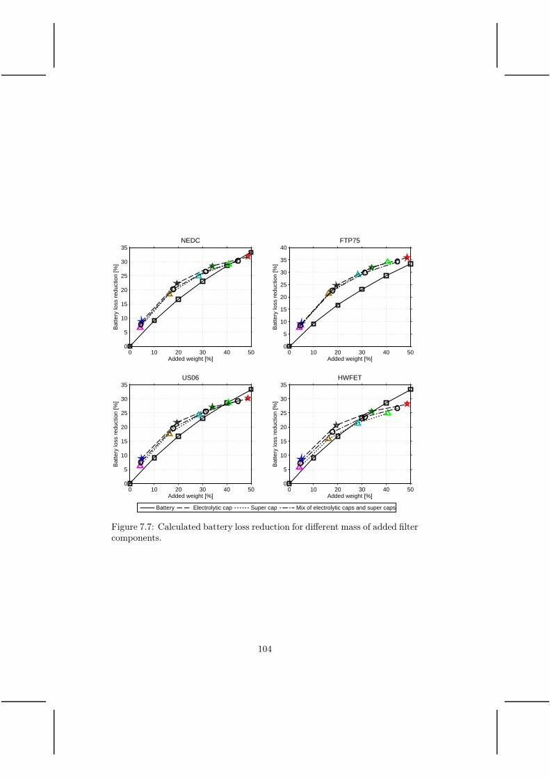
0 10 20 30 40 500
5
10
15
20
25
30
35NEDC
Added weight [%]
Bat
tery
loss
red
uctio
n [%
]
0 10 20 30 40 500
5
10
15
20
25
30
35
40FTP75
Added weight [%]
Bat
tery
loss
red
uctio
n [%
]
0 10 20 30 40 500
5
10
15
20
25
30
35US06
Added weight [%]
Bat
tery
loss
red
uctio
n [%
]
0 10 20 30 40 500
5
10
15
20
25
30
35HWFET
Added weight [%]
Bat
tery
loss
red
uctio
n [%
]
Battery Electrolytic cap Super cap Mix of electrolytic caps and super caps
Figure 7.7: Calculated battery loss reduction for different mass of added filtercomponents.
104
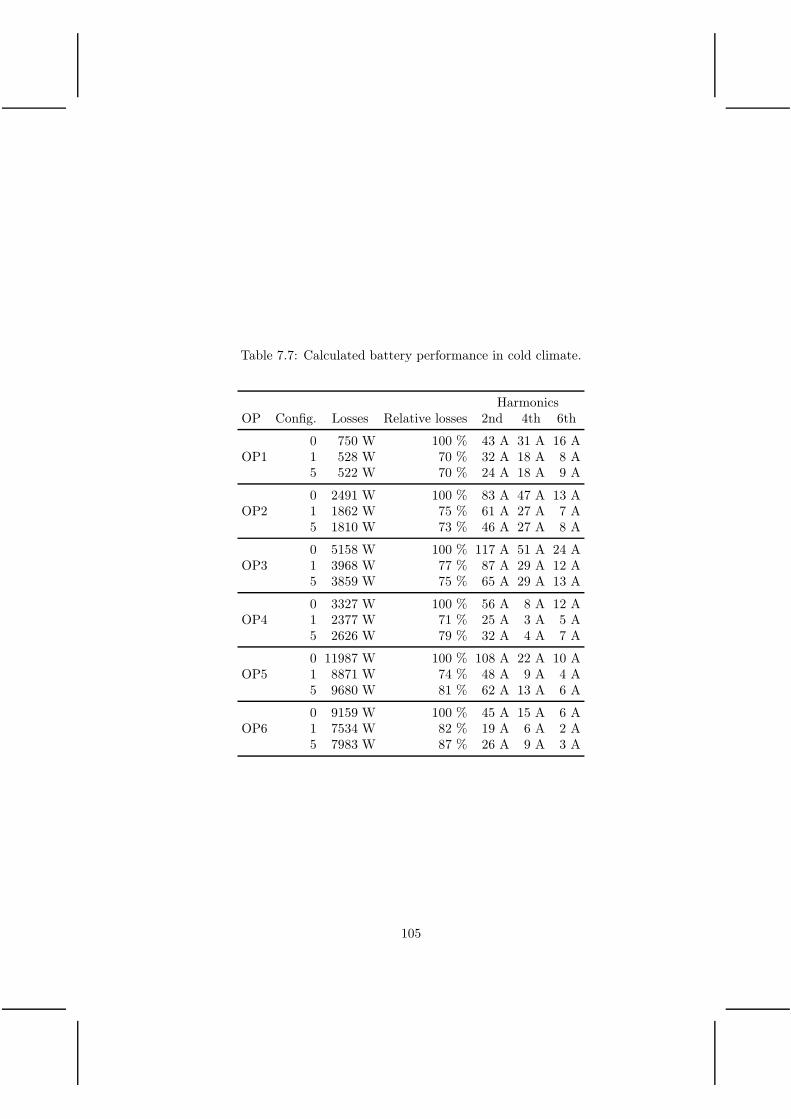
Table 7.7: Calculated battery performance in cold climate.
HarmonicsOP Config. Losses Relative losses 2nd 4th 6th
OP10 750 W 100 % 43 A 31 A 16 A1 528 W 70 % 32 A 18 A 8 A5 522 W 70 % 24 A 18 A 9 A
OP20 2491 W 100 % 83 A 47 A 13 A1 1862 W 75 % 61 A 27 A 7 A5 1810 W 73 % 46 A 27 A 8 A
OP30 5158 W 100 % 117 A 51 A 24 A1 3968 W 77 % 87 A 29 A 12 A5 3859 W 75 % 65 A 29 A 13 A
OP40 3327 W 100 % 56 A 8 A 12 A1 2377 W 71 % 25 A 3 A 5 A5 2626 W 79 % 32 A 4 A 7 A
OP50 11987 W 100 % 108 A 22 A 10 A1 8871 W 74 % 48 A 9 A 4 A5 9680 W 81 % 62 A 13 A 6 A
OP60 9159 W 100 % 45 A 15 A 6 A1 7534 W 82 % 19 A 6 A 2 A5 7983 W 87 % 26 A 9 A 3 A
105

106
Chapter 8
Proposal for packaging of
the inverter-battery unit and
its cooling circuit
Traditionally, the inverter and battery are placed separately in the vehicle.Two separate cooling circuits are often used to cool the inverter and thebattery since the battery should be operated at a cooler temperature. Whenusing a multilevel inverter, a suggestion here is to place the inverter insidethe battery and incorporate it into the already existing CVMM (Cell VoltageMonitoring Module), which are already in place in an electrified vehicle tomonitor and balance the battery cells but also to measure the temperature.
The thermal impedance of the battery pack has a very long time constant,therefore it is not the peak battery loss that is of interest but the severalminute average loss. Here, an average of one minute is used to find themaximum battery cooling need. This time constant is on the shorter side,so the analysis is made to be on the safe side. When designing the system,to ensure that the drive system does not get over heated, the vehicle shouldnot be operated at high loads for a too long time period, see Fig. 8.1. If thisoccurs, then either the requirements of the vehicle must be reduced or theelectrical components must be enlarged. To determine the maximum averagebattery loss, the US06 drive cycle is used since it is the most demandingamong the four drive cycles analysed. The one minute base average batteryloss during this drive cycle can be seen in Fig. 8.2.
As expected from Chapter 5, it can be noted that the MLI has substan-tially higher battery losses compared to the TLI for the 50 km driving rangetest vehicle.
107
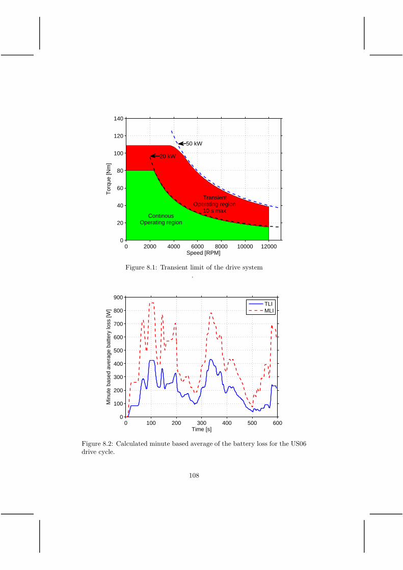
0 2000 4000 6000 8000 10000 120000
20
40
60
80
100
120
140
Speed [RPM]
Tor
que
[Nm
]
20 kW
50 kW
TransientOperating region
10 s maxContinous
Operating region
Figure 8.1: Transient limit of the drive system.
0 100 200 300 400 500 6000
100
200
300
400
500
600
700
800
900
Time [s]
Min
ute
base
d av
erag
e ba
ttery
loss
[W]
TLIMLI
Figure 8.2: Calculated minute based average of the battery loss for the US06drive cycle.
108
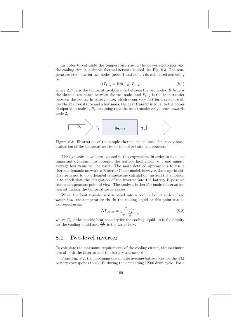
In order to calculate the temperature rise in the power electronics andthe cooling circuit, a simple thermal network is used, see Fig. 8.3. The tem-perature rise between two nodes (node 1 and node 2)is calculated accordingto
∆T1−2 = Rth1−2 · P1−2 (8.1)
where ∆T1−2 is the temperature difference between the two nodes, Rth1−2 isthe thermal resistance between the two nodes and P1−2 is the heat transferbetween the nodes. In steady state, which occur very fast for a system withlow thermal resistance and a low mass, the heat transfer is equal to the powerdissipated in node 1, P1, assuming that the heat transfer only occurs towardsnode 2.
T1 T2RT 1-21
Figure 8.3: Illustration of the simple thermal model used for steady stateevaluation of the temperature rise of the drive train components.
The dynamics have been ignored in this expression. In order to take oneimportant dynamic into account, the battery heat capacity, a one minuteaverage loss value will be used. The more detailed approach is to use athermal dynamic network, a Foster or Cauer model, however, the scope in thischapter is not to do a detailed temperature calculation, instead the ambitionis to check that the integration of the inverter into the battery is possiblefrom a temperature point of view. The analysis is therefor made conservative,overestimating the temperature increases.
When the heat transfer is dissipated into a cooling liquid with a fixedwater flow, the temperature rise in the cooling liquid at this point can beexpressed using
∆Twater =Pwater
Cp · ∆V∆t · ρ
(8.2)
where Cp is the specific heat capacity for the cooling liquid , ρ is the densityfor the cooling liquid and ∆V
∆t is the water flow.
8.1 Two-level inverter
To calculate the maximum requirements of the cooling circuit, the maximumloss of both the inverter and the battery are needed.
From Fig. 8.2, the maximum one minute average battery loss for the TLIbattery corresponds to 433W during the demanding US06 drive cycle. For a
109
water flow of 6 liters per minute, the temperature rise in the battery coolingcircuit is given by
∆TwaterTLIbattery=PTLIbattery
Cp · ∆V∆t · ρ
= 1.1 K (8.3)
where Cp = 3770 Jkg K , ρ = 1.036 kg/l and ∆V
∆t = 0.1 l/s for a mixtureconsisting of 50 % water and 50 % ethylene glycol.
For the IGBT inverter used for the TLI system, which has a very smallmass and has to be able to dissipate the loss immediately (on a second basis)to the cooling fluid, the maximum loss is equal to 1180 W and can be notedin the loss map for the TLI system, see Fig. 5.1. With the same water flow,the temperature increase for the water cooling circuit at the inverter wouldbe equal to
∆TwaterTLIinverter=PTLIinverter
Cp · ∆V∆t · ρ
= 3.0 K (8.4)
at the worst operating point.
For a standard electrified vehicle, the cooling circuit for the electric ma-chine and power electronics typically hace a macimum temperature of 65 C.According to the data sheet of the IGBT module, the thermal resistance perIGBT leg is equal to 0.1 K/W . With a water temperature of 65 C thejunction temperature in the IGBT modules would be
TjunctionTLIinverter= RthJ−water ·
PTLIinverter
3+ 65 = 105 C (8.5)
which is an acceptable temperature, 20 C below the maximum recommendedvalue.
8.2 MOSFET equipped cell voltage monitor mod-
ules
When using a MLI instead of a TLI, the inverter consists of several modulesthat do not have to be placed as one unit. It is chosen here to place theH-bridges inside the battery, and the battery must of course be made slightlylarger to support the additional H-bridges. In addition, the cooling circuitof the battery has to be upgraded with a higher flow, in order to handle theincreased battery loss level.
A simple sketch of the proposed H-bridge inverter is shown in Fig. 8.4.In this picture, only the MOSFETs, the PCB and a heat sink is shown.In a real H-bridge inverter additional hardware is of course needed such asconnectors, gate drivers and a processor etc. It is assumed that they can be
110

fitted between the MOSFETS. In Fig. 8.5 the H-bridge module from Fig.8.4 is mounted on the already existing CVMM. It can be noted that the sizeincrease is moderate compared to the original CVMM. The volume of the 9added inverters is equal to 1.4 l (calculated from the measurements in Fig.8.5), to be compared with over 100 l for a 10 kWh battery. Even though theyare to be incorporated into the already existing battery circuit, the volumemust be somewhat more increased due to an additional cooling need in thebattery compartment. The extra cooling need will be determined in Section8.2.5.
It should be noted that even though the MOSFETs do not have a massto low pass filter the power loss, the PCB board and heat sink does. Inthe following analysis the PCB and heat sink is assumed to have a very lowmass to be on the safe side in the analysis. This means that the maximuminstantaneous (over one fundamental period) inverter loss is considered whencomparing the temperature rise from junction to heat sink.
Figure 8.4: Proposed H-bridge inverter together with air cooled heat sink,one out of nine in the battery. Five MOSFETs are placed at each switchlocation, resulting in a total of 20 MOSFETs for each H-bridge.
Figure 8.5: CVMM module with incorporated inverter and added heat sink.
111

Figure 8.6: CVMM module with incorporated inverter together with batterymodule (150 cells).
112

8.2.1 Thermal resistance of the MOSFETs
The thermal resistance from the junction of the transistors to the case isaccording to the data sheet 0.5 K/W . Since 20 transistors share the sameloss (average over one fundamental period), the H-bridge equivalent thermalresistance from the junctions to the PCB board becomes
RthJ−C = 0.025 K/W (8.6)
when referring to the total H-bridge loss.
8.2.2 Thermal properties of the PCB
From the bottom side of the PCB, the heat flow must go through the wholePCB towards the heat sink. According to [56], the design of the copperlayer has a very small influence of the thermal conductivity through thePCB, which instead is totally dominated by the glass fiber. Usually thePCB used is often FR4. According to the measurements done by [56] thethermal resistivity for heat conduction through an FR4 PCB is 0.29 W
m Kwhich would be too much for the design configuration illustrated in Fig.8.4. However, if Metal-Core PCB (MCPCB) is used instead, the thermalresistivity is reduced significantly. In [57], the thermal resistance through a1.5 mm PCB is calculated to 0.2 K/W for a board of 270 mm2. The boardin Fig. 8.4 has an area of 12500 mm2, a factor of 46 higher, resulting in athermal resistance of
RthC−H = 0.004 K/W (8.7)
between the equivalent transistor cases and the backside of the PCB.
8.2.3 Heat sink for CVMM
If the inverter loss would be dissipated through an air cooled heat sink, aheat sink is placed to cover the whole backside of the PCB. To calculate thethermal resistance of such a heat sink, data from a smaller available heat sinkis used and extrapolated to the right geometry. Here, the heat sink "ICKSMD B 10 SA" from Fischer Elektronik GmbH is used [58] with a thermalresistance of 35 K/W for an area of 190 mm2. The heat sink in Fig. 8.4 hasan area of 12500mm2, a factor of 66 higher, resulting in a thermal resistanceof
RthH−A = 0.53 K/W (8.8)
from the back side of the PCB to ambient air.
If instead the water cooling circuit of the battery is used to dissipate theheat from the power electronic, the thermal resistance would be even lower
113

than the air cooled heat sink, this would lead to a temperature rise from thejunction of the transistors relative to the cooling water temperature of onlya few degrees, which would be no problem at all, since the cooling fluid in abattery is typically low, at maximum 40 C. Similarly as in (8.3), the watertemperature would due to the MOSFET losses only rise
∆TwaterMLIinverter=PMLIinverter
Cp · ∆V∆t · ρ
= 0.7 K (8.9)
since the inverter loss are very low for the multilevel inverter case.
8.2.4 Cooling circuit temperature increase due to bat-tery losses
The worst case battery loss when using a multilevel inverter without any filtercapacitances to propel the vehicle is according to Fig. 8.2 equal to 860 Wwhen considering the minute based average. The temperature rise for a waterflow of 6 liters per minute can then be calculated in the same way as in (8.3)and corresponds to
∆TwaterMLIbattery=PMLIbattery
Cp · ∆V∆t · ρ
= 2.2 K (8.10)
for the MLI case.
8.2.5 Resulting thermal analysis for the MOSFET-enhancedCVMM system
The total thermal resistance from the junction of the transistors to ambientair becomes
RthJ−A = 0.025 + 0.004 + 0.53 = 0.56 K/W (8.11)
when considering the total H-bridge loss for an air cooled inverter. The max-imum inverter loss is according to Fig. 5.5 equal to 280 W . This means thatevery H-bridge has to dissipate of 280/9 = 31 W , the junction temperaturewill rise above ambient temperature with
∆TJ−A = RthJ−A · PH−bridge = 0.56 · 31 = 18 K (8.12)
which is such a low temperature increase the it can be considered to be onthe edge of over dimensioning.
A worst case scenario could be that one H-bridge has to deliver all thepower. This happens if there is a very serious unbalance in the battery pack,
114

and the control system decides to use one H-bridge more than the others.If the output voltage is low at this instance, it could be that one H-bridgehas to deliver all the power since only one H-bridge should be activated tocreate the desired voltage. That would lead to that the junction temperatureincreases to 18 · 3 = 54 K above the ambient temperature in the batterycompartment, which is still fully acceptable.
When using a water cooled inverter mounted at the battery, the loss fromboth systems increases the water temperature. The temperature differencebetween the input and output will for this case be equal to
∆TwaterMLItotal= ∆TwaterMLIbattery
+∆TwaterMLIinverter= 2.9 K (8.13)
using (8.10) and (8.9) for the worst operating points.
8.3 Slim sized inverters
If the slim sized inverters presented in Section 5.4 are to be used, both thelosses and the thermal performance of the system would change. For theslim sized TLI using the FS400 IGBT module, the inverter losses remainquite constant compared to the TLI with the FS800. However, the thermalresistance from the junction to the water is increased from RthJ−water =0.1 K/W to RthJ−water = 0.2 K/W according to the data sheet. Thiswould according to (8.5) result in a junction temperature of roughly
TjunctionTLIinverter= RthJ−water ·
PTLIinverter
3+ 65 = 144 C (8.14)
which is an unacceptable continuous temperature for the inverter if a goodreliability is to be guaranteed. A degrading of the vehicle performance wouldhave to be incorporated for some extreme occasions.
For the slim sized MLI case, the number of semiconductors is halved at thesame time as the losses are about doubled. The equivalent thermal resistancefrom the junction of the 10 MOSFETs placed on each PCB then becomes
RthJ−C = 0.05 K/W. (8.15)
Since the PCB and heat sink has the same size and performance the re-sulting thermal resistance from the junctions of the 10 MOSFETs to ambientair becomes
RthJ−A = 0.05 + 0.004 + 0.53 = 0.59 K/W. (8.16)
which is just a slight increase since the thermal resistance from the heatsink to ambient air is the dominating part. With a worst case power loss of
115

PH−bridge = 560/9 = 62 W per H-bridge, the junction temperature rise fromambient air temperature would be
∆TJ−A = RthJ−A · PH−bridge = 0.59 · 62 = 36 K. (8.17)
This is definitely acceptable even if the ambient air is very warm. One shouldalso keep in mind that the heat sink has a thermal mass due to its size. Sincethe largest part of the thermal resistance is between the heat sink and ambientair, the MLI setup can withstand much higher losses for a short period oftime than the steady state calculated ones.
116

Chapter 9
Conclusions
The investigation of using multilevel inverters (MLI) in electrified vehicles(EVs) shows that this inverter type has a great potential from an efficiencypoint of view. By reducing the voltage steps applied to the electric machine,as well as the switching frequency and slew rates, the EMI in the motor phasecables are reduced. The power loss in the power electronics is reduced due tothe possibility to use the MOSFET technology and a system where the powerelectronics is placed in the already existing battery voltage measurementmodules is proposed. These modules are placed inside the battery casingbut since the losses are low, the heat dissipation of the power electronics caneasily be dealt with either with internal air cooling and/or conduction intothe already existing water cooling circuit for the battery.
Due to three separate single-phase systems, the battery modules are sub-ject to a current with the second harmonic of the motor frequency. Thisincreases the losses in the battery, especially at operating points where a lotof reactive power flowing in the electric machine is present. The drive cycleanalysis shows that during most drive cycles the MLI drive system is thebeneficial choice from a loss perspective compared to the TLI. In the com-monly used NEDC the total inverter-battery losses are reduced with 30 %and in the in USA commonly used FTP75 by 23 % when using a batterywith an energy content of only 10 kWh and without any filter capacitors.Only during the highly dynamic US06, the accumulated loss energy is larger(by 11 %) for the MLI system compared to the classical two-level invertersystem.
If a larger battery with an energy content of 40 kWh is used, the batteryloss is reduced, and the MLI system shows an even greater performance andpotential due to that the battery losses are no longer dominant. For theNEDC drive cycle, the loss reduction is now as large as 75 % and for the
117

demanding US06 around 47 % when using the MLI system without filtercapacitors compared to the TLI system for the combined battery-inverterlosses.
Since the MLI forces very uneven waveforms in the battery it was neededto use a more detailed battery model compared with the case when a TLIsystem is investigated. Several models has been developed, parameterisedand verified and by using a Randles model consisting of three poles andthree zeros, the best accuracy was achieved. The selected battery model wasexperimentally verified and shows a good match to the measurements overa wide range of operating points. For the MLI system, a 30 % reduction ofthe predicted battery loss is achieved compared to using a purely resistivebattery model. This is mainly due to the filtering effect of the double layercapacitance in the battery cell.
By placing capacitors to the input of the H-bridges in the MLI system,the battery current ripple is reduced. For low speed driving, super capaci-tors improves the performance more than using electrolytic capacitors, andat high speed driving the low resistance electrolytic capacitors are the mostbeneficial choice for a certain added mass. In the investigated examples, froma loss perspective, it is always beneficial to add a certain mass of capacitorscompared to adding more battery cells (up to extreme limits), which could fa-cilitate the cooling of the battery in addition to enhancing the driving range.For a cold battery the advantages are even larger since capacitors does notincrease their inner resistance at all as much compared to the increase in thebattery cells. This leads to that the performance at cold climate is signifi-cantly improved, even with a small amount of filter capacitors. Furthermore,worth mentioning is that by adding capacitors, the EMI spectrum from thebattery cable and cells is also significantly lowered.
To sum up, from the energy efficiency point of view as well as from thepackaging point of view, the MLI system shows a good potential comparedto the TLI system.
118

Chapter 10
Future Work
This thesis has addressed and analysed some aspects of the possibility to usea multilevel inverter in electrified vehicles instead of the two-level unverter.However, some aspects and topics need further investigations in order todetermine the suitability of the system. Following is a list of proposed inves-tigations.
• With a MLI the possibility to take out other voltage levels can bemade. One level can for example directly supply the 12 V systemand the MLI could still make sure that this level is balanced with theremaining levels. The vehicle could then be made cheaper, since noDC/DC converter would be needed. The need for galvanic insulationin this case could on the other hand be a problem and needs furtherinvestigation.
• Investigate how the performance of a MLI would be when using morelevels. What is the optimum for different drive cycles and car sizes?
• At low frequencies or at 0 Hz, the machine can not operate with selec-tive harmonic elimination due to that the motor current would not besinusoidal. Investigation about when it is necessary to start using PWMis accordingly needed. Since the MOSFETs has much lower switchinglosses, it could be beneficial use PWM at all speeds, without increasingthe losses very much.
• The MLI has the opportunity to control from which modules the energyshould be taken from, it can therefore also be used to control where thelosses takes place. If one inverter or battery becomes too hot the MLIcan be controlled to use this level less. Investigation about how thiscontrol can be made, and the benefits from it can be of interest.
119

• If a switch and/or in the MLI malfunctions, and is detected, the invertercan be controlled to keep operating without using that level, makingthe MLI a fault tolerant system. In vehicles this is a very importantfeature and investigation about the subject is of great interest.
• Investigation about different modulation strategies is of great impor-tance. Reference [59] and [60] for example, show that space vectormodulation is an alternative for MLI and shows good performance.
• Since the MLI can choose from which battery groups the energy shouldbe taken from, it could be beneficial to compose the battery storagefrom different sorts of batteries and maybe even super capacitors. Forvery urban drive cycles it could be beneficial to use the super capacitorsfor acceleration and deceleration, and use the batteries as the averageenergy supply, reducing the losses.
• The economical analysis as well as life cycle analysis of having a MLIsystem instead of a TLI system are needed.
120

References
[1] R. Roy and J. Ghouili, “Numerical simulation of a multipowered onboarddrive train,” in Electrical and Computer Engineering, 2004. CanadianConference on, vol. 4, may 2004, pp. 2069 – 2072 Vol.4.
[2] S. Imai, N. Takeda, and Y. Horii, “Total efficiency of a hybrid electricvehicle,” in Power Conversion Conference - Nagaoka 1997., Proceedingsof the, vol. 2, aug 1997, pp. 947 –950 vol.2.
[3] M. Ceraolo, A. di Donato, and G. Franceschi, “A general approach toenergy optimization of hybrid electric vehicles,” Vehicular Technology,IEEE Transactions on, vol. 57, no. 3, pp. 1433 –1441, may 2008.
[4] N. Mutoh, Y. Hayano, H. Yahagi, and K. Takita, “Electric brakingcontrol methods for electric vehicles with independently driven frontand rear wheels,” Industrial Electronics, IEEE Transactions on, vol. 54,no. 2, pp. 1168 –1176, april 2007.
[5] D. Gao, C. Mi, and A. Emadi, “Modeling and simulation of electric andhybrid vehicles,” Proceedings of the IEEE, vol. 95, no. 4, pp. 729 –745,april 2007.
[6] J. Wu, A. Emadi, M. Duoba, and T. Bohn, “Plug-in hybrid electric vehi-cles: Testing, simulations, and analysis,” in Vehicle Power and Propul-sion Conference, 2007. VPPC 2007. IEEE, sept. 2007, pp. 469 –476.
[7] P.-S. Kim, “Cost modeling of battery electric vehicle and hybrid electricvehicle based on major parts cost,” in Power Electronics and Drive Sys-tems, 2003. PEDS 2003. The Fifth International Conference on, vol. 2,nov. 2003, pp. 1295 – 1300 Vol.2.
[8] C. Chan, “The state of the art of electric, hybrid, and fuel cell vehicles,”Proceedings of the IEEE, vol. 95, no. 4, pp. 704 –718, april 2007.
[9] C. Chan and Y. Wong, “The state of the art of electric vehicles tech-nology,” in Power Electronics and Motion Control Conference, 2004.IPEMC 2004. The 4th International, vol. 1, aug. 2004, pp. 46 –57 Vol.1.
121

[10] C. Chan and K. Chau, “Power electronics challenges in electric vehicles,”in Industrial Electronics, Control, and Instrumentation, 1993. Proceed-ings of the IECON ’93., International Conference on, nov 1993, pp. 701–706 vol.2.
[11] J. Miller, “Power electronics in hybrid electric vehicle applications,” inApplied Power Electronics Conference and Exposition, 2003. APEC ’03.Eighteenth Annual IEEE, vol. 1, feb. 2003, pp. 23 –29 vol.1.
[12] Z. Shen and I. Omura, “Power semiconductor devices for hybrid, electric,and fuel cell vehicles,” Proceedings of the IEEE, vol. 95, no. 4, pp. 778–789, april 2007.
[13] F. Peng, W. Qian, and D. Cao, “Recent advances in multilevel con-verter/inverter topologies and applications,” in Power Electronics Con-ference (IPEC), 2010 International, 2010, pp. 492–501.
[14] M. Jongerden and B. Haverkort, “Which battery model to use?” Soft-ware, IET, vol. 3, no. 6, pp. 445 –457, december 2009.
[15] M. Einhorn, F. Conte, C. Kral, and J. Fleig, “Comparison, selection,and parameterization of electrical battery models for automotive appli-cations,” Power Electronics, IEEE Transactions on, vol. 28, no. 3, pp.1429–1437, March 2013.
[16] G. Plett, “High-performance battery-pack power estimation using a dy-namic cell model,” Vehicular Technology, IEEE Transactions on, vol. 53,no. 5, pp. 1586–1593, Sept 2004.
[17] B. Enache, E. Lefter, and C. Stoica, “Comparative study for generic bat-tery models used for electric vehicles,” in Advanced Topics in ElectricalEngineering (ATEE), 2013 8th International Symposium on, May 2013,pp. 1–6.
[18] Z. Zheng, K. Wang, L. Xu, and Y. Li, “A hybrid cascaded multilevelconverter for battery energy management applied in electric vehicles,”Power Electronics, IEEE Transactions on, vol. 29, no. 7, pp. 3537–3546,July 2014.
[19] R. Kroeze and P. Krein, “Electrical battery model for use in dynamicelectric vehicle simulations,” in Power Electronics Specialists Conference,2008. PESC 2008. IEEE, june 2008, pp. 1336 –1342.
[20] A. Shafiei, A. Momeni, and S. Williamson, “Battery modeling approachesand management techniques for plug-in hybrid electric vehicles,” in Ve-hicle Power and Propulsion Conference (VPPC), 2011 IEEE, sept. 2011,pp. 1 –5.
122

[21] A. Hentunen, T. Lehmuspelto, and J. Suomela, “Electrical battery modelfor dynamic simulations of hybrid electric vehicles,” in Vehicle Power andPropulsion Conference (VPPC), 2011 IEEE, Sept 2011, pp. 1–6.
[22] L. Y. Wang, M. P. Polis, G. Yin, W. Chen, Y. Fu, and C. Mi, “Batterycell identification and soc estimation using string terminal voltage mea-surements,” Vehicular Technology, IEEE Transactions on, vol. 61, no. 7,pp. 2925–2935, Sept 2012.
[23] J. Groot, State-of-Health Estimation of Li-ion Batteries: Cycle Life TestMethods. Licentiate Thesis, Chalmers University of Technology, 2012.
[24] S. Haghbin, K. Khan, S. Lundmark, M. Alaküla, O. Carlson, M. Leksell,and O. Wallmark, “Integrated chargers for ev’s and phev’s: examples andnew solutions,” in Electrical Machines (ICEM), 2010 XIX InternationalConference on, sept. 2010, pp. 1 –6.
[25] L. Tolbert, F. Peng, and T. Habetler, “Multilevel inverters for electricvehicle applications,” in Power Electronics in Transportation, 1998, oct1998, pp. 79 –84.
[26] A. Verma, P. Thakura, K. Jana, and G. Buja, “Cascaded multilevelinverter for hybrid electric vehicles,” in Power Electronics (IICPE), 2010India International Conference on, jan. 2011, pp. 1 –6.
[27] O. Josefsson, A. Lindskog, S. Lundmark, and T. Thiringer, “Assessmentof a multilevel converter for a phev charge and traction application,”in Electrical Machines (ICEM), 2010 XIX International Conference on,sept. 2010, pp. 1 –6.
[28] O. Josefsson, T. Thiringer, S. Lundmark, and H. Zelaya, “Evaluationand comparison of a two-level and a multilevel inverter for an ev usinga modulized battery topology,” in IECON2012, 2012.
[29] M. Dahidah and V. Agelidis, “Selective harmonic elimination multilevelconverter control with variant dc sources,” in Industrial Electronics andApplications, 2009. ICIEA 2009. 4th IEEE Conference on, may 2009,pp. 3351 –3356.
[30] E. Guan, P. Song, M. Ye, and B. Wu, “Selective harmonic eliminationtechniques for multilevel cascaded h-bridge inverters,” in Power Elec-tronics and Drives Systems, 2005. PEDS 2005. International Conferenceon, vol. 2, nov. 2005, pp. 1441 – 1446.
[31] W. Shuanghong, Z. Qionghua, M. Zhiyuan, and Z. Libing, “Implementa-tion of a 50 kw 4-phase switched reluctance motor drive system for hev,”in Electromagnetic Launch Technology, 2004. 2004 12th Symposium on,may 2004, pp. 518 – 522.
123

[32] (2013, Feb.) Tesla motors. [Online]. Available: http://www.teslamotors.com/roadster/technology/motor
[33] Y. Guan, Z. Zhu, I. Afinowi, J. Mipo, and P. Farah, “Design of syn-chronous reluctance and permanent magnet synchronous reluctance ma-chines for electric vehicle application,” in Electrical Machines and Sys-tems (ICEMS), 2014 17th International Conference on, Oct 2014, pp.1853–1859.
[34] M. Ehsani, K. Rahman, and H. Toliyat, “Propulsion system design ofelectric and hybrid vehicles,” Industrial Electronics, IEEE Transactionson, vol. 44, no. 1, pp. 19 –27, feb 1997.
[35] J. Lindström, Development of an ExperimentalPermanent-Magnet Mo-tor Drives. Licentiate Thesis, Chalmers University of Technology, 1999.
[36] J. Hellsing, Design and Optimization of a Permanent Magnet Motor fora Hybrid Electric Vehicle. Licentiate Thesis, Chalmers University ofTechnology, 1998.
[37] C. Du-Bar, Design of a fault-tolerant fractional slot PMSM for a vehicleapplication. Licentiate Thesis, Chalmers University of Technology, 2014.
[38] I. Khan, “Battery chargers for electric and hybrid vehicles,” in PowerElectronics in Transportation, 1994. [Proceedings], oct 1994, pp. 103 –112.
[39] L. Tolbert, F. Z. Peng, T. Cunnyngham, and J. Chiasson, “Charge bal-ance control schemes for cascade multilevel converter in hybrid electricvehicles,” Industrial Electronics, IEEE Transactions on, vol. 49, no. 5,pp. 1058 – 1064, oct 2002.
[40] M. Yilmaz and P. T. Krein, “Review of battery charger topologies, charg-ing power levels, and infrastructure for plug-in electric and hybrid vehi-cles,” Power Electronics, IEEE Transactions on, vol. 28, no. 5, pp. 2151–2169, may 2013.
[41] L. Wang, J. Liang, G. Xu, K. Xu, and Z. Song, “A novel battery chargerfor plug-in hybrid electric vehicles,” in Information and Automation(ICIA), 2012 International Conference on, june 2012, pp. 168 –173.
[42] F. Lacressonniere and B. Cassoret, “Converter used as a battery chargerand a motor speed controller in an industrial truck,” in Power Electronicsand Applications, 2005 European Conference on, 0-0 2005, pp. 7 pp. –P.7.
124

[43] D.-G. Woo, G.-Y. Choe, J.-S. Kim, B.-K. Lee, J. Hur, and G.-B. Kang,“Comparison of integrated battery chargers for plug-in hybrid electricvehicles: Topology and control,” in Electric Machines Drives Conference(IEMDC), 2011 IEEE International, may 2011, pp. 1294 –1299.
[44] P. Haaf and J. Harper, “Diode reverse recovery and its effect on switchinglosses,” unpublished. [Online]. Available: http://www.fairchildsemi.com/onlineseminars/diodeReverseRecoverySwitchingLosses.pdf
[45] D. Graovac and M. Pürschel, “Igbt power losses calculationusing the data-sheet parameters,” unpublished. [Online]. Available:http://www.element14.com/community/servlet/JiveServlet/download/20553-1-3493/IGBT\%20Power\%20Losses\%20Calculation\%20using\%20the\%20Data\%20Sheet\%20Parameters.pdf
[46] J. Jose, G. Goyal, and M. Aware, “Improved inverter utilisation usingthird harmonic injection,” in Power Electronics, Drives and Energy Sys-tems (PEDES) 2010 Power India, 2010 Joint International Conferenceon, dec. 2010, pp. 1 –6.
[47] A123Systems, “Datasheet, battery cell anr26650m1a,” unpublished.[Online]. Available: http://e-motion.lt/wp-content/uploads/2010/01/ANR26650M1A_Datasheet.pdf
[48] RIFA/KEMET, “Datasheet, electrolytic capacitor peh169gd5220q,”unpublished. [Online]. Available: http://www.kemet.com/
[49] Ioxus, “Datasheet, super capacitor rsc2r7107sr,” unpublished. [Online].Available: http://www.ioxus.com/
[50] Infineon, “Datasheet, fs800r07a2e3,” unpublished. [Online]. Avail-able: http://www.infineon.com/dgdl/Infineon-FS800R07A2E3-DS-v03_00-en_de.pdf?fileId=db3a304320d39d590121b0581fc82d8d
[51] ——, “Datasheet, ipb025n10n3g,” unpublished. [Online]. Avail-able: http://www.infineon.com/dgdl/Infineon-IPB025N10N3G-DS-v02_03-en.pdf?fileId=db3a30431ce5fb52011d1ab1d9d51349
[52] I. Rectifier, “Datasheet, irf1324s-7ppbf,” unpublished. [Online].Available: http://www.irf.com/product-info/datasheets/data/irf1324s-7ppbf.pdf
[53] V. Schwarzer and R. Ghorbani, “Drive cycle generation for design opti-mization of electric vehicles,” Vehicular Technology, IEEE Transactionson, vol. 62, no. 1, pp. 89–97, Jan 2013.
125

[54] General Administration of Quality Supervision, “GB/T 18387-2008:Limits and test method of electric and magnetic field strength fromelectric vehicles, 9 kHz to 30 MHz,” National Standard of the People’sRepublic of China, China, Standard, Sept 2008.
[55] A. Narula, “Modeling of ageing of lithium-ion battery at low temperat-uras,” 2014, 60.
[56] K. Azar and J. Graebner, “Experimental determination of thermal con-ductivity of printed wiring boards,” in Semiconductor Thermal Measure-ment and Management Symposium, 1996. SEMI-THERM XII. Proceed-ings., Twelfth Annual IEEE, Mar 1996, pp. 169–182.
[57] I. Cree, “Optimizing pcb thermal performance for cree R© xlamp R©leds,” unpublished. [Online]. Available: www.cree.com/xlamp_app_notes/pcb_thermal
[58] F. E. GmbH, “Datasheet, ick smd b 10 sa,” unpublished. [Online].Available: http://www.fischerelektronik.de/
[59] X. Hou, Y. Li, and Y. Liu, “A novel general space vector modulationalgorithm for multilevel inverter based on imaginary coordination,” inPower Electronics and Drive Systems, 2003. PEDS 2003. The Fifth In-ternational Conference on, vol. 1, nov. 2003, pp. 392 – 396 Vol.1.
[60] Y. Li, Y. Gao, and X. Hou, “A general svm algorithm for multilevel con-verters considering zero-sequence component control,” in Industrial Elec-tronics Society, 2005. IECON 2005. 31st Annual Conference of IEEE,nov. 2005, p. 6 pp.
126