Investigating the Suitability of UV/Vis Spectrophotometric Methods for Analyzing Arsenic in Urban Soils for use in Undergraduate Laboratory Courses

A Senior Honors Thesis

Presented in Partial Fulfillment of the Requirements for graduation with research distinction in Chemistry in the undergraduate colleges of The Ohio State University

by

Christine Pellegrini

The Ohio State University June 2010

Project Advisor: Assistant Professor Ted M. Clark, Department of Chemistry

ABSTRACT

Quantifying the concentration of arsenic in soil samples is important for many

environmental chemistry investigations, including those characterizing heavy metal in

urban settings and examining anthropogenic contributions. Although several approaches

for quantifying arsenic in environmental samples have been reported, many of these are

poorly suited for use in undergraduate teaching laboratories. The use of UV-Vis

spectrophotometric methods are, for both logistical and pedagogical reasons, well-suited

for inclusion in the chemistry curriculum. Within this investigation two UV-Vis

spectrophotometric methods have been examined to ascertain their applicability for use at

the undergraduate level. Criteria for inclusion in chemistry courses, such as time

constraints, reproducibility, reagent stability, and dynamic range have been considered

for a method employing a Leuco-malachite green dye (Revanasiddappa, 2007) or a

method involving a Rhodamine B dye (Pillai, 2000). These two methods were examined

in conjunction with two different soil digestion procedures for the analysis of soil

samples collected from Columbus, OH. An investigation of the Leuco-malachite green

method strongly suggests that it is ill-suited for the analysis of arsenic Columbus’ soil

due to interference from iron. The Rhodamine B method, in contrast, is less affected by

iron or chromium interferrents and statistical analysis indicates good agreement between

this method and X-ray fluorescence spectrophotometric analysis. However, poor

precision in the Rhodamine B method, attributed in part to the digestion scheme,

indicates that additional work is required before this method is included in undergraduate

courses.

1

ACKNOWLEDGEMENTS

To my advisor, Dr. Ted M. Clark, thank you for letting me have the opportunity

to pursue this project. Thank you for your willingness to offer great scientific insight and

for your generous approachability. Finally, thank you for your enthusiasm which

encouraged me to continue on with the project even when I felt frustrated.

I would also like to thank Brittany Poast, whose listening ear, resourcefulness,

and encouragement was invaluable. Without you, I also would probably not felt as

inclined to clean up after myself in the lab.

I also owe a great deal of thanks to the REEL research group, especially

undergraduates Jason Eng, Jason Stybel, and Steven Kiracofe, as well as the participating

students. You not only provided me with over 300 soil samples to work with, but an

extra pair of hands in the lab.

2

TABLE OF CONTENTS ABSTRACT 1

Page

ACKNOWLEDGEMENTS 2 TABLE OF CONTENTS 3 LIST OF FIGURES & TABLES 4

Chapter 1 – INTRODUCTION 1.1 – Overview 6 1.2 – Project Description 9

Chapter 2 – EXPERIMENTAL METHODS 2.1 – Malachite Green Procedure 18 2.2 – Rhodamine B Procedure 19 2.3 – Soil Sample Preparation 19 2.4 – UV-Vis Analysis 21 Chapter 3 – RESULTS & DISCUSSION 3.1 – Overview 22 3.2 – Malachite Green Calibration 23 3.3 – Rhodamine B Calibration 26 3.4 – Identifying Potential Contaminants 32 3.5 – Iron Interference in Malachite Green Procedure 33 3.6 – Chromium Interference in Malachite Green Procedure 34 3.7 – Masking Effects of EDTA 35 3.8 – Iron Interference in Rhodamine B Procedure 37 3.9 – Soil Digestion Comparison with Rhodamine B 38 3.10 – Limiting Variation within Cherian Method 42 3.11 – Soil Digestion Parameters for Cherian Method 43 Chapter 4 – CONCLUSIONS 45 Chapter 5 – FUTURE WORK 47 APPENDICES: SUGGESTED CLASSROOM PROCEDURES Appendix A – Malachite Green 48 Appendix B – Rhodamine B 50 Appendix C – Cherian Soil Digestion 52 Appendix D – EPA Method 3050b 53 REFERENCE LIST 54

3

4

LIST OF FIGURES Page

Fig. 1 Distribution of soil collection sites in Greater Columbus, OH. 10

Fig. 2 Histograms showing Fe, Ti, Pb, Zn, and As concentrations 12

Fig. 3 Leuco-malachite green reaction mechanism 14

Fig. 4 Azure B reaction mechanism 15

Fig. 5 Rhodamine B reaction mechanism 15

Fig. 6 Absorption Spectra for Malachite green 24

Fig. 7 Malachite green calibration from 0.05 to 10 ppm 25

Fig. 8 Malachite green calibration from 0.09 to 1.2 ppm 26

Fig. 9 Three calibration curves of Rhodamine B 27

Fig. 10 Rhodamine absorption and pH effect 30

Fig. 11 The degradation of the Rhodamine B curve 32

Fig. 12 Malachite green and iron interference at low ppm 33

Fig. 13 Malachite green and iron interference at high ppm 34

Fig. 14 Malachite green and chromium interference 35

Fig. 15 The binding of EDTA to metals. 36

Fig. 16 Rhodamine B and iron interference 37

Fig. 17 Variability of Cherian soil digestion method 41

Fig. 18 Bulk and surface analysis of Pb with XRF and FAAS. 42

LIST OF TABLES Page

Table 1. Descriptive statistics of analytes present in top-soil 12

collected from urban parks as determined by XRF.

Table 2. Acceptable analytical mediums as tested by the methods 16

of Revanasiddappa, Pillai, and Cherian.

Table 3. Criteria for inclusion of an analytical method in a testing 23

laboratory versus a classroom.

Table 4. Accepted tolerance values for selected instrumentation 28

and glassware.

Table 5. Individual uncertainties within Rhodamine B method. 29

Table 6. Percent relative uncertainty for individual flasks of Rhodamine 29

B Calibration.

Table 7. Effects of HCl amount used and reflux duration on amount 44

of arsenic extracted.

5

INTRODUCTION 1.1 – OVERVIEW

Arsenic is found in more than 200 different inorganic minerals, occurs frequently

as trivalent (arsenite) or pentavalent (arsenate) ions, and can bind to organic material

commonly present in the environment. Arsenic is mobile and found in the Earth’s

sediment, soil, and water. In addition to being present at naturally occurring levels,

arsenic is frequently found at higher concentrations due to anthropogenic contributions,

including pesticides, herbicides, industrial waste, and the burning of fossil fuels (Mandal,

2002; Mattschullat, 2000). The health concerns associated with arsenic are well known

and, in the general public, the word arsenic is readily associated with a poison. Chronic

exposure to arsenic, which occurs most commonly though contaminated drinking water,

has serious health effects including gastrointestinal damage, and skin and internal

cancers. Among its various forms, inorganic arsenic species are known to be more toxic

than the organic ones, and As(III) is more toxic than As(V) (Quaghebeur, 2005; Alvarez-

Benedi, 2005).

The level of arsenic in uncontaminated soils from various countries range from

0.01 to 40 mg kg-1 (ppm), but varies considerably among geographic regions

(Mattschullat, 2000). Researchers have investigated arsenic at different types of sites,

including locations with identified anthropogenic contamination (Chirenje, 2003),

locations that are representative urban environments (Craul, 1985), and locations that

represent minimal anthropogenic contributions, i.e. background concentrations (Chen,

2001).

6

Given the importance of arsenic in the environment, various instrumental

approaches have been used to determine its concentration, including atomic absorption

spectroscopy, X-ray fluorescence spectroscopy, neutron activation analysis, and

inductively coupled plasma (Mandal, 2002). In addition to these techniques, which are

costly and require trained analysts, researchers are interested in developing alternate

methods that make use of ultraviolet or visible (UV/Vis) light spectroscopy (Cherian,

2005; Pillai, 2000; Revanasiddappa, 2007). These alternate UV/Vis spectroscopic

methods utilize the same inexpensive instrumentation but differ with respect to the

chemical reactions completed in the procedure, e.g. the use of Leuco-malachite green,

Azure-B, or Rhodamine B are all possible dyes that may be used.

Although UV/Vis spectroscopic methods have many potential advantages

including ease of use, low-cost, etc., it has not been determined if a UV/Vis spectroscopic

method is suitable for the determination of arsenic in urban soils that exhibit diverse

compositions. This is a major shortcoming since such samples are of great interest for

many “real world” investigations, particularly those in the developing world (Mandal,

2002).

UV/Vis spectroscopic methods, in addition to widespread use in quantitative

testing methods, are of course extremely common in undergraduate and high school

chemistry laboratory courses. Indeed, UV/Vis spectroscopy is a workhorse approach that

is well-suited for both commonplace (Casey and Tatz, 2007) and innovative (Grannas

and Lagalante, 2010) laboratory experiments. UV/Vis spectrometers are robust, relatively

inexpensive, and frequently used to introduce students to many topics, e.g. Beer’s Law

(Muyskens and Sevy, 1997), color (Suding and Buccigross, 1994) instrument calibration

7

and spectroscopy (Casey and Tatz, 2007), that it is difficult to envision introductory

chemistry laboratory courses without their inclusion. In recently published general

chemistry textbooks UV/Vis spectrometers are also described, although their inclusion

here often occurs in passing (1 page being the norm) and in quite different topic areas

such as the Bohr atom (Petrucci, 2007), chemical kinetics (Tro, 2008; Brown, LeMay,

Bursten, 2006), and spectrophotometric measurements (Silberberg, 2006). In some

textbooks this material is relegated to an appendix (Zumdahl and Zumdahl, 2009) or not

explicitly described (Brady and Senese, 2009; Burdge, 2009; Masterton and Hurley,

2009). Overall, this suggests a scenario in which UV/Vis spectrometers play an

important role in chemistry laboratory courses but with varied treatment in the lecture

portion of their respective courses.

Beyond their inclusion in traditional laboratory courses, UV/Vis spectroscopic

methods have also proven to be highly valued in courses that include an in-class research

component. In the Research Experiences to Enhance Learning (REEL) program, for

example, a very wide variety of environmentally relevant soil and water samples have

been analyzed by UV/Vis spectroscopic methods and dozens of these in-class student-led

projects have been communicated at REEL symposia and at the Central Regional

American Chemical Society (CERMACS) conference over the last four years.

The inclusion of a UV/Vis spectrophotometric method for the determination of

arsenic in soil samples requires consideration of multiple factors since criteria for

incorporating an analysis methodology in a teaching laboratory may differ from those

accompanying its incorporation in an analytical testing laboratory. Although several

UV/Vis spectrophotometric methods have appeared in the literature it is not clear if any

8

of them are suitable for use by a large number of novice users in an in-class research

setting in which the research results “count”, i.e. the research results are intended to be of

research quality and suitable for dissemination online, in posters, papers, etc., and are not

simply learning exercises.

The primary goal of this investigation is to investigate the suitability of different

reported analytical chemistry protocols for the analysis of arsenic in urban soils with the

intention of incorporating an optimized protocol in undergraduate courses (such as

general chemistry or analytical chemistry) that may be involved in in-class environmental

research projects. Both the construction of external calibration curves and the digestion

of soil samples will be considered. Attention will be given to those factors that support

or inhibit the inclusion of such a procedure on a very large scale, i.e. 200-300 students in

a 3 week period. In addition, an overview of the characteristics of soil in Greater

Columbus, OH will be provided since particular soil attributes (such as the presence of

interferrents) may deleteriously affect a given analysis procedure.

1.2 – PROJECT DESCRIPTION

An extensive suite of soil samples has been collected throughout the Greater

Columbus area by students in the REEL program. These soil samples have been

collected from sites intended to either represent the baseline anthropogenic contribution

in this area or to answer student-specific research questions. In a typical spring quarter

more than 300 samples are collected, processed, and analyzed by X-ray fluorescence

spectroscopy (XRF). As shown in Figure 1, the level of contamination (in this case for

lead) often has a spatial correlation that is most likely related to historical patterns of land

use.

9

10

Low lead (<80 ppm)

Moderate lead (80 to 150 ppm)

High lead (> 150 ppm)

Fig. 1 Distribution of soil collection sites in Greater Columbus, OH. Relative Pb concentrations are shown. Area shown encompasses approximately 50 mi2.

X-ray fluorescence spectroscopy is very well-suited for the analysis of soil

samples since it provides a rapid analysis of multiple elements in a non-destructive

manner. Portable X-ray fluorescence units are now available in a price range ($20k to

$40k) that makes their inclusion in educational settings feasible. Table 1 includes

descriptive statistics for analytes present in soil samples collected from parks by students

in the REEL program as determined by XRF.

Histograms showing the concentration of elements Fe, Ti, Pb and Zn present in

these urban park samples are included in Figure 2. These histograms indicate that

elements like Fe and Ti are well above the detection limit of this XRF spectrometer,

while elements like Pb and Zn are near their detection limit; the limit of detection for Pb

and Zn are both near 10-15 ppm.

Several important analytes that may be present in soils samples are, unfortunately,

are not easily analyzed by a portable XRF spectrometer. Arsenic, for example, has a

limit of detection near 15-20 ppm when analyzed by an Innov-X Alpha XRF

spectrometer. In addition, the signal from lead and arsenic overlap making analysis

problematic when lead is present in appreciable quantities (like the soil samples described

here). As shown in Figure 2, the concentration of arsenic in soils collected in Greater

Columbus is very near the limit of detection and in a typical suite more than 50% of the

samples are unable to be analyzed by XRF.

11

Table 1. Descriptive statistics of analytes present in top-soil collected from urban parks as determined by XRF. Samples collected in spring of 2009, N~200. Element (ppm) Mean Median St.

dev. Range Minimum Maximum Skewness Kurtosis

Fe 29809 29718 7402 75884 9712 85596 2.211 15.876 Ti 4247 4276 837 5888 858 6746 -0.629 2.059 Mn 461 439 186 955 136 1091 0.730 0.555 Zr 237 236 51 316 61 377 -0.255 0.592 Zn 210 151 304 3088 60 3148 6.687 53.682 Sr 125 113 52 448 86 644 6.460 54.618 Rb 85 87 14 100 25 125 -0.786 2.248 Pb 79 42 139 1592 16 1609 7.683 76.237

Fig. 2. Histograms showing the concentration of Fe, Ti, Pb, Zn, and As in urban park soil collected in Greater Columbus, OH and analyzed by XRF spectroscopy.

Iron

0

0.05

0.1

0.15

0.2

0.25

0.3

0.35

10 20 30 40 50 60 70 80 90 100

Fe (%), 5% bin size

No

rma

lize

d F

req

uen

cy

Titanium

0

0.02

0.04

0.06

0.08

0.1

0.12

0.14

0.16

0.18

500 1500 2500 3500 4500 5500 6500

Ti (ppm), 250 ppm bin size

No

rma

lize

d F

req

ue

ncy

Arsenic

0

0.05

0.1

0.15

0.2

0.25

0.3

0.35

0.4

0.45

20 30 40 50

As (ppm), 5 ppm bin size

No

rma

lize

d F

req

ue

ncy

Lead

0.00

0.10

0.20

0.30

0.40

0.50

0.60

0 50 100 150 200 250 300 350 400 450

Pb (ppm), 25 ppm bin size

No

rma

lize

d F

requ

ency

Zinc

0

0.05

0.1

0.15

0.2

0.25

0.3

0.35

0 200 400 600 800 1000 1200

Zn (ppm), 50 ppm bin size

No

rma

lize

d F

req

ue

ncy

12

When testing samples for heavy metals a common instrumental alternative to

XRF analysis is the use of a flame atomic absorption spectrophotometer (FAAS). For

FAAS measurements the sample is introduced into a flame and atomized. The fuel used

in FAAS is usually a combination of air and acetylene, and the flame reaches

temperatures between 2100-2400 degrees C. A light beam is directed through the flame

and reaches a detector that determines the amount of light that was absorbed by the

atomized element in the flame. Each element has a characteristic absorption wavelength

and a radiation source (a hollow-cathode lamp) that produces the light with the desired

wavelength. In the case of arsenic, radiation in the ultraviolet region of the

electromagnetic spectrum at 193.7 nm is used. Although the instrument sensitivity of

FAAS is capable of determining arsenic at the part per million (ppm) level, it has a

limited dynamic range and displays a Beer’s Law relationship between approximately 0.5

and 25 ppm. For this reason, significant sample dilution and optimization is often

required (Skoog, 1998).

The fact that arsenic’s wavelength with maximum absorption is 193.7 nm is

unfortunate since an air-acetylene flame intensely absorbs ultraviolet radiation thereby

reducing the instrument’s sensitivity. For this reason an alternate approach is often

adopted, i.e. converting arsenic to arsine gas, AsH3 (g), which is then swept into a quartz

cell and heated by the flame. The air-acetylene flame is still used but it now only serves

as a convenient source of heat. Although this approach offers the possibility of increased

sensitivity, considerable instrument optimization is required and this approach is not

included in any undergraduate laboratory courses in the Chemistry department at OSU

and appears ill-suited for use in general chemistry courses. For these reasons the current

13

investigation has considered UV/Vis spectroscopy as an alternative to both FAAS and

XRF.

A common feature of many UV/Vis protocols (for arsenic other analtyes) is to

have a reagent react quantitatively with the analyte so that a colored compound is formed.

Often, for a dilute solution, a Beer’s Law relationship will then be present in which the

amount of the analyte (in this case arsenic) and the resulting absorbance of light at a

specific wavelength are directly correlated. Since the measurement of this absorbance is

readily accomplished with a UV/Vis spectrometer, the key step in this procedure is the

manner in which the reagent (often a dye) reacts with the analyte.

A procedure that uses Leuco-malachite green (LMG) in UV/Vis arsenic

determinations has been reported (Revanasiddappa, 2007). The structure of LMG is

shown in Figure 3. In this procedure, arsenic (III) reacts with potassium iodate in

hydrochloric acid medium to liberate iodine quantitatively. The liberated iodine

selectively oxidizes LMG to the Malachite green dye (MG), which is blue green in color.

Fig. 3 Proposed reaction mechanism for conversion of Leuco-malachite green to Malachite green (from Revanasiddappa, 2007).

A procedure that employs azure B in UV/Vis arsenic determinations has also been

developed (Cherian, 2005). This method also involves the liberation of iodine by the

reaction of arsenic (III) with potassium iodate in an acidic medium. The liberated iodine

14

then bleaches the violet color of azure B, as measured at 644 nm. The proposed reaction

is shown in Figure 4.

15

Another closely related procedure has been proposed by Pillai and co-workers

(Pillai, 2000). In their work arsenic (III) is once again reacted with acidified potassium

iodate to liberate iodine. The liberated iodine bleaches the pinkish red color of

Rhodamine-B, which is measured spectrophotometrically at 556 nm. The proposed

reaction is shown in Figure 5.

Fig. 4 Proposed reaction mechanism for conversion of Azure B (from Cherian, 2005).

Fig. 5 The reaction pathway for the bleaching of Rhodamine B (from Pillai, 2000).

Each of methods has reported usage with environmentally and/or biologically

relevant samples. The results from such method validation investigations are typically

reported either as the concentration determined or as a percent recovery. In situations

where the original amount of arsenic is zero or near zero, the sample is spiked by adding

a known amount of arsenic to the matrix. The amount recovered is then expressed as a

percent recovery based on the amount determined relative to the amount added. In

samples containing a quantifiable amount of arsenic, samples are commonly tested

without additional analyte being introduced, although in some situations these samples

are also spiked with a known amount and a percent recovery calculated. A description of

different samples examined by the three spectrophotometric methods noted above is

included in Table 2. Among these findings, most relevant for the current investigation is

the analysis of soil samples. As shown in Table 2, the Azure B method has been applied

for soil samples with arsenic present at the low ppm-level, the Rhodamine-B method

applied for soil samples with approximately 10-15 ppm arsenic, and the Leuco-malachite

green methods applied for soil samples with close to 200 ppm arsenic.

Table 2. Acceptable analytical matrices for arsenic and UV-Vis Spectrophotometry (Revanasiddappa, 2007; Pillai, 2000; and Cherian, 2005).

Method

Matrix Leuco-malachite green Azure B Rhodamine B

Conc. (ppm)

% Recovery

Conc. (ppm)

% Recovery Conc. (ppm) %

Recovery Ground Water

0.385 spiked with 0.2 100 ---- ---- 0.298-0.503

spiked with 0.2-0.4 98.9

Polluted Water

0.544 spiked with 0.2 99.5 1.05-2.04 ---- 0.300-0.514

spiked with 0.2-0.4 98.9

Soil 187.2 spiked with 50 99.8 1.36-1.58 ---- 11.0-14.2 ----

Spinach Leaves

49.1 spiked with 25 99.6 ---- ---- 14.1-16.2 ----

Tomato Leaves

50.7 spiked with 25 100.2 ---- ---- 15.1-17.6 ----

Hair ---- ---- 3.00-7.00 99.5 2.00-4.00 96.7 Nail ---- ---- 2.00-4.00 98.9 2.00-4.00 96.5

Urine ---- ---- 3.00-7.00 99.5 2.00-4.00 97.5 Serum ---- ---- 3.00-7.00 99.7 2.00-4.00 96.0

Zinc Ore ---- ---- ---- ---- 0.29-0.40 98.0

16

Although these reported procedures have been refined in earlier investigations, an

unsettled question is their sensitivity when interfering ions also present, especially those

(shown in Table 1) prevalent in the soils of Columbus. As will be discussed below, the

effectiveness of a particular methodology in terms of probable interferrents is but one

criterion applicable for determining the utility of an analytical approach prior to its

inclusion in a classroom setting.

17

EXPERIMENTAL METHODS

2.1 – MALACHITE GREEN PROCEDURE

A 0.05% stock solution of Leuco-malachite green (LMG) was prepared by adding

25 mg of LMG ([4-((4-(dimethylamino)phenyl)(phenyl)methyl)-N,N-dimethyl

benzenamine]), 100 mL distilled water and 1.5 mL of 85% phosphoric acid to a 500 mL

volumetric flask with shaking until the dye dissolved. The contents were then brought to

volume. Stock solutions of 2% potassium iodate and 0.45M hydrochloric acid were

created from solid potassium iodate and a certified 3M solution of hydrochloric acid. An

acetate buffer with a pH of 4.5 was created by dissolving 13.6 g of sodium acetate

trihydrate in distilled water in a 100 mL volumetric flask, with pH adjustments made by

acetic acid. A 4 ppm stock solution of sodium arsenite was created through dilution from

a 1000 ppm certified sodium arsenite solution.

In 50 mL volumetric flasks, aliquots of arsenic (III) ranging from 0.08 ppm to 1.2

ppm were added for the production of a calibration curve or a 1 mL of digested sample

for soil analysis, followed by 5 mL of 0.45M hydrochloric acid and 2.5 mL of potassium

iodate. After two minutes of gentle shaking, 2.5 mL of 0.05% LMG was added followed

by 10 mL of acetate buffer.

All solutions were certified to be at a pH of 4.5 ± 0.2 with a pH meter. Any

corrections to pH were made with dilute sodium hydroxide or 0.45M hydrochloric acid.

The solutions were heated to 40 degrees C in a water bath for five minutes to hasten

complete color development. Once the solutions were cooled to room temperature they

were brought to volume with distilled water. All absorbance measurements were made at

617 nm.

18

2.2 – RHODAMINE B PROCEDURE

A 0.2% solution of Rhodamine B ([9-(2-carboxyphenyl)-6-diethylamino-3-

xanthenylidene]-diethylammonium chloride) was prepared by dissolving 2.5 mg of

Rhodamine B in distilled water in a 100 mL volumetric flask. Stock solutions of 2%

potassium iodate and 0.45M hydrochloric acid were prepared from solid potassium iodate

and a certified 3M solution of hydrochloric acid. A 4 ppm stock solution of sodium

arsenite was prepared by diluting a 1000 ppm certified sodium arsenite solution.

In 50 mL volumetric flasks, aliquots of arsenic (III) ranging from 0.08 ppm to 1.2

ppm were added for the construction of a calibration curve followed by 1 mL of 0.45M

hydrochloric acid and 2 mL of potassium iodate. For soil samples, 1 mL of the digested

sample was mixed with 2 mL of potassium iodate. After two minutes of gentle shaking,

the pH was taken with a pH meter. The pH was adjusted with dilute sodium hydroxide

and 0.45M hydrochloric acid so that the pH was 6.5 ± 2.0. Then, 2 mL of 0.2%

Rhodamine B was added. The solutions were allowed to stand for 20 minutes to ensure

complete color development. The solutions were then brought to volume and analyzed at

556 nm.

2.3 – SOIL SAMPLE PREPARATION

The majority of the soil samples utilized were collected from a variety of local

parks in the city of Columbus, Ohio. The remaining soil samples used were certified by

the Resource Technology Corporation to contain a known amount of arsenic, catalog

numbers CRM022, CRM028, CRM030, CRM033, and CRM034.

An abbreviated soil digestion method proposed by Cherian (Cherian & Narayana,

2005) was followed by adding 5 mL of concentrated hydrochloric acid to a 1 g sample of

19

soil that had been dried and finely ground. The extract was removed and three more 5

mL portions of hydrochloric acid were added with subsequent removals of the extract.

The extract was refluxed for 30 minutes and cooled to room temperature. The extract

was added to a 50 mL volumetric flask containing 15 mL of distilled water. Drops of

10% KI were added to the solution until the presence of excess iodine is evidenced by the

production of a reddish brown color. Any excess iodine is destroyed by the addition of

ascorbic acid. The solution was brought to volume and stored in a cool and dark place

when not in use.

The second digestion method was followed in accordance with EPA Method

3050b. A 1 g dried and finely ground soil sample is mixed with 10 mL of concentrated

nitric acid and refluxed at about 95 degrees C for 10-15 minutes. Additional 5 mL

portions of concentrated nitric acid are added to the cooled sample and refluxed at 95

degrees C for 30 minutes until the addition of nitric acid does not produce brown fumes

as evidence of continuing oxidation. The solution is then refluxed for two hours. Once

the solution has been cooled to room temperature, 2 mL of distilled water and 3 mL of

30% hydrogen peroxide are added and the solution is warmed until effervescence ceases.

Additional 1 mL portions of hydrogen peroxide are added followed by heating until the

effervescence upon addition ceases or becomes negligible. No more than 10 mL of

hydrogen peroxide is added in total. The solution is refluxed for an additional two hours

and allowed to cool. 10 mL of concentrated hydrochloric acid is added followed by 15

minutes of refluxing. After the solution cools to room temperature, it is filtered through

no. 41 Whatman Filter paper into a 100 mL volumetric flask and brought to volume with

distilled water.

20

2.4 – UV-VIS ANALYSIS

For the Malachite green calibration, a Jenway 6320D digital spectrophotometer

was used to record the absorbance in 1.0 cm quartz cells. For all other absorbance

measurements, including the Rhodamine B calibration, interference testing, and soil

analysis an OceanOptics ISS/UV-Vis spectrophotometer was utilized in tandem with

OceanOptics software using 1.0 cm quartz cells. The absorbance spectrum was recorded

from 300-890 nm.

21

RESULTS AND DISCUSSION

3.1 – OVERVIEW

Methods for the determination of analytes in environmentally relevant samples

should meet certain standards, e.g. high reproducibility and short analysis time, when

situated in testing laboratories. When used in classroom settings, however, the criteria

for judging an analytical methodology must take into account additional constraints.

When including authentic research experiences in undergraduate courses key

considerations for analytical methods include laboratory logistics, the quality of student

results, pedagogical value, and student engagement and decision-making. In terms of the

analytical method examined here, i.e. the determination of arsenic in soil samples by

UV/Vis spectroscopy, these concerns manifest themselves in three areas, including 1)

construction of a calibration curve, 2) the effect of likely interferrents, and 3) the

digestion of soil samples. As shown in Table 3, criteria for inclusion of an analytical

method in a testing laboratory, i.e. a facility operated by trained technicians, are not

identical with those for a classroom.

22

Table 3. Criteria for inclusion of an analytical method in a testing laboratory versus a classroom.

Topic Testing Laboratory Criteria Classroom Criteria

General

considerations

1. Reproducibility 2. Time (high throughput) 3. Safety 4. Cost 5. Waste

1. Reproducibility 2. Time (suitable for constrained

class time) 3. Safety 4. Cost 5. Waste

Construction of calibration curve

6. Wide dynamic range 7. Sufficient sensitivity, limit

of detection 8. Stability of calibration

curve.

6. Wide dynamic range. Deviations from Beer’s law are problematic if a very low concentration is required.

7. Sufficient sensitivity, limit of detection

8. Preparation and stability of reagents on a weekly or bi-weekly schedule since classes may meet only once or twice each week.

Interferrents

9. Chemical pre-treatment to remove interferrents must be feasible. Instrumental separations must be adequate.

9. Chemical pre-treatment to remove interferrents must be feasible and sufficient. Instrumental separation approaches are unlikely to be used.

Soil digestion

10. Quantitative extraction of desired analyte.

10. Quantitative extraction of desired analyte.

11. Time. 12. Safety.

3.2 – MALACHITE GREEN CALIBRATION

According to the Beer-Lambert Law, absorbance is linear with concentration

where A = εbc with ε and b representing the molar absorptivity and pathlength,

respectively. The molar absorptivity describes the amount of light absorbed at a

particular wavelength for a given substance. A greater molar absorptivity results in a

greater absorbance of the substance. The linear relationship between concentration and

23

absorbance is most applicable with dilute solutions (≤0.01 M). At higher concentrations

a significant deviation from linearity is commonly observed as shown by a gradual

saturation in a calibration curve. This is held to occur because molecules in solution

cease to behave independently of each other as concentration increases. Complications

can also arise when the range of linearity occurs at extremely low concentrations due to

sensitivity issues. This is an important consideration in classroom settings that are more

prone to contamination of glassware at the low ppm-level.

The Malachite green solutions are blue-green in color and have a peak absorbance

at 617 nm. The peak associated with Malachite green is easily distinguished, as shown in

Figure 6 when a solution that is 0.8 ppm in arsenic is compared with distilled water.

0

0.05

0.1

0.15

0.2

0.25

0.3

500 520 540 560 580 600 620 640 660 680 700

Wavelength (nm)

Abs

orba

nce

a b

Fig. 6 Absorption Spectra for distilled water (a) and the Malachite gdye (b) in 0.8 ppm arsenic (III) solution.

reen

The calibration curve of Malachite green is consistent with a Beer’s Law

relationship when the arsenic concentration is quite low (<0.5 ppm) and has dynamic

range extending to approximately 1.5 ppm. At concentrations greater than 1.2 ppm there

24

is clear deviation from a linear response as displayed in Figure 7, which shows the

absorbance of malachite green solutions containing 0.05-10 ppm of arsenic at a

wavelength of 617 nm. A closer examination Figure 8 more closely displays the range of

linearity at the same wavelength. Yet even this example of the linear range shows

significant negative deviation from Beer’s Law. This attests to the inherent sensitivity of

the method which shows signs of saturation even at an absorbance of 0.33 and

concentration up to 1.2 ppm (1.6 x 10-8 M). This would be problematic in a classroom

because the sensitivity is high and the calibration curve could be easily nullified by any

small errors made by undergraduate students.

Fig. 7 Absorbance of Malachite green from 0.05 to 10 ppm at 617 nm.

25

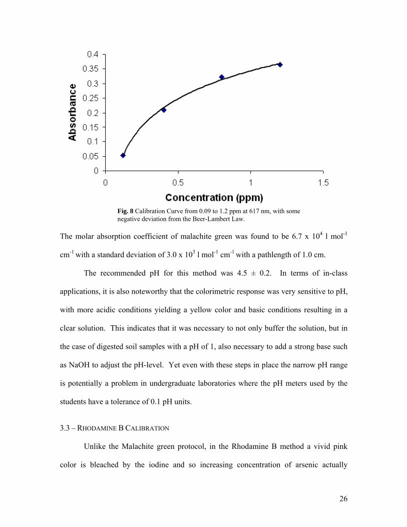
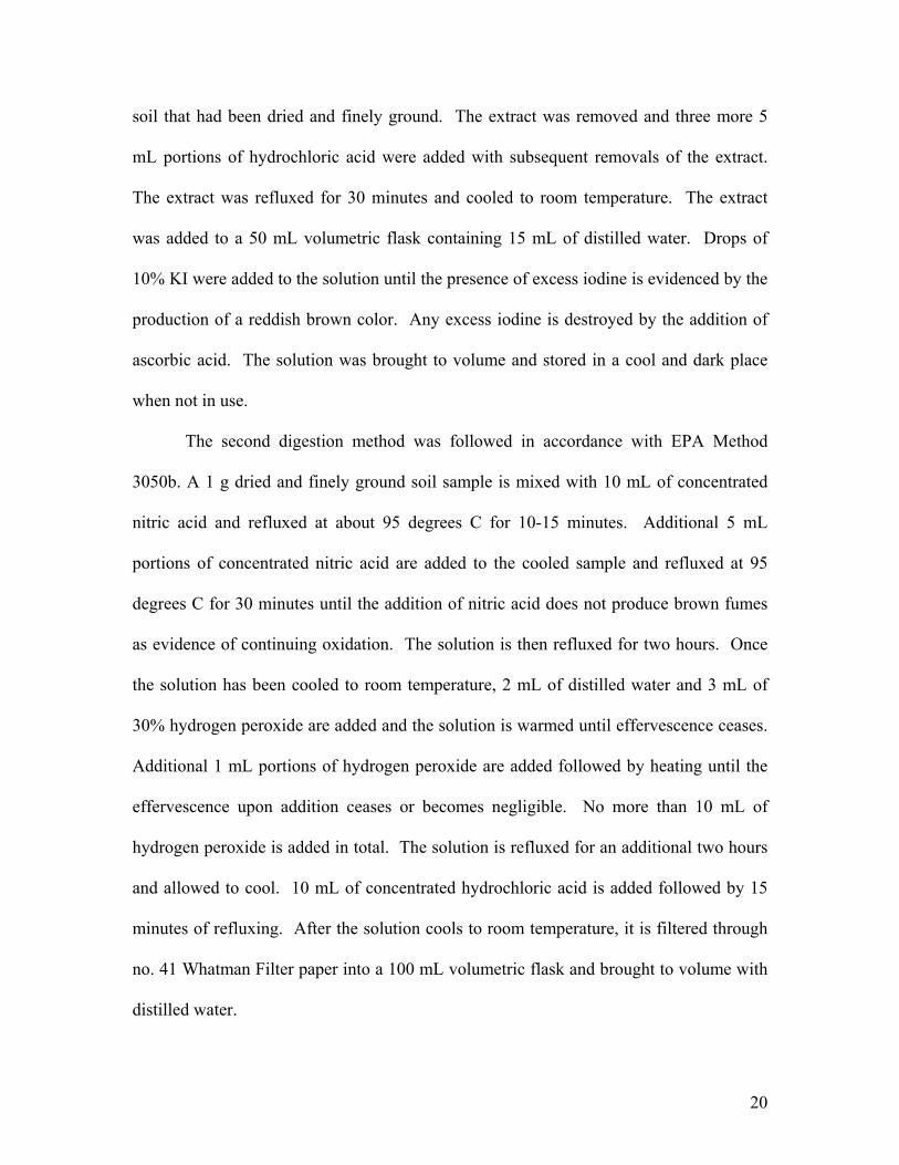
Fig. 8 Calibration Curve from 0.09 to 1.2 ppm at 617 nm, with some negative deviation from the Beer-Lambert Law.

The molar absorption coefficient of malachite green was found to be 6.7 x 104 l mol-1

cm-1 with a standard deviation of 3.0 x 103 l mol-1 cm-1 with a pathlength of 1.0 cm.

The recommended pH for this method was 4.5 ± 0.2. In terms of in-class

applications, it is also noteworthy that the colorimetric response was very sensitive to pH,

with more acidic conditions yielding a yellow color and basic conditions resulting in a

clear solution. This indicates that it was necessary to not only buffer the solution, but in

the case of digested soil samples with a pH of 1, also necessary to add a strong base such

as NaOH to adjust the pH-level. Yet even with these steps in place the narrow pH range

is potentially a problem in undergraduate laboratories where the pH meters used by the

students have a tolerance of 0.1 pH units.

3.3 – RHODAMINE B CALIBRATION

Unlike the Malachite green protocol, in the Rhodamine B method a vivid pink

color is bleached by the iodine and so increasing concentration of arsenic actually

26

decreases the absorbance of Rhodamine B. While this behavior is somewhat unusual, it

does not mean that the Beer Law does not apply; the absorbance is still proportional to

the concentration of analyte in solution. It should be noted that the bleaching of the

Rhodamine B is not able to be witnessed visually, since the decrease in absorbance is

slight and the original color is very vibrant.

The calibration curve for Rhodamine B was found to have a range of linearity

from about 0.08 ppm to 0.4 ppm. The method proposed by Pillai suggested a range of

0.04 ppm to 0.4 ppm, but it was observed here that concentrations below 0.08 ppm were

below the limit of detection. To investigate the robustness of this method multiple

calibration curves were prepared. As shown in Figure 9, the calibration curves are linear

between approximately 0.15 and 0.4 ppm and, like the Malachite green method, exhibit a

narrow dynamic range that may prove problematic when situated in a classroom setting.

Fig. 9 Three independently created calibration curves of Rhodamine B at 556 nm showing the percent relative uncertainty in concentration and the inherent uncertainty of the spectrometer.

27

The degree of reproducibility was examined more closely by calculating error

bars applicable for each datum shown in Figure 9. Within Figure 9, the y-axis error bars

demonstrate the uncertainty inherent in the spectrometer. The x-axis error bars included

in Figure 9 reflect a 2% relative uncertainty in the concentration of arsenic, which is

higher than the actual value for the sake of visibility. The percent relative uncertainty is

determined based on the uncertainty of both arsenic and Rhodamine. Unlike other

scenarios where the only relevant uncertainty is in the analyte concentrations, the

uncertainty present in the concentration of the dye is also relevant considering that the

dye is bleached rather than activated by the analyte. The uncertainty in the

concentrations of arsenic and Rhodamine B is attributable to the tolerances of the

glassware and analytical balance used in the preparation. Table 4 shows the tolerances of

the glassware and balance.

Table 4. Accepted tolerance values for selected instrumentation and glassware.

Instruments Tolerance Class 1 Analytical Balance ±0.01 mg Class A Volumetric Flasks

50 mL ±0.05 mL 100 mL ±0.08 mL

Class A Transfer Pipets 1 mL ±0.006 mL 2 mL ±0.006 mL 5 mL ±0.01 mL 25 mL ±0.03 mL

The percent relative uncertainty of each measurement is determined by the

division of the tolerance by the amount measured multiplied by 100. The percent relative

28

uncertainty is useful when propagating error from calculations requiring multiplication or

division. The individual uncertainties from the procedure are shown in Table 5.

Sources of Error % Relative Uncertainty Rhodamine Stock Solution Mass Uncertainty 0.40 Transfer Uncertainty 0.31 Arsenic Stock 1.00 Arsenic Stock Dilution 0.62 Arsenic Dilution in 0.08 ppm 0.61 Arsenic Dilution in 0.16 ppm 0.32 Arsenic Dilution in 0.24 ppm 0.30 Arsenic Dilution in 0.36 ppm 0.22 Arsenic Dilution in 0.40 ppm 0.22

The total uncertainty in a series of measurements is calculated by the following

formula, where e represents the individual uncertainties.

% total error = √Σ(%e2)

The total percent error for each flask of arsenic is shown in Table 6.

Table 5. Individual uncertainties within Rhodamine B method.

Table 6. Percent relative uncertainty for individual flasks of Rhodamine B Calibration.

Total % Uncertainty 0.08 ppm flask 1.42 0.16 ppm flask 1.32 0.24 ppm flask 1.31 0.32 ppm flask 1.30 0.40 ppm flask 1.30

By these calculations the percent uncertainty for each sample of arsenic is less than 1.5%.

This supports the high degree of reproducibility demonstrated in Figure 9. In fact, the

tolerance of the UV-Vis Spectrometer has a greater uncertainty than the concentration of

29

each sample. The high degree of reproducibility is very important in a classroom setting

where multiple students are creating calibration curves in the same environment and with

the same samples. Obviously, it is necessary to have a method that shows uniformity

from student to student.

The molar absorptivity for Rhodamine B was calculated to be 9.3 x 104 l mol-1

cm-1 with a standard deviation of 2.0 x 103 l mol-1 cm-1. The maximum absorbance

occurred near 556 nm. The reported method suggested a suitable pH range of 6.5 ± 2.0

which is much wider than the range required for malachite green suggesting easier

implementation for use in undergraduate courses. All samples were adjusted to this range

with NaOH.

Since the digested soil samples are highly acidic, the absorbance spectra of a 0.16

ppm solution of arsenic in Rhodamine B were compared at pH readings of 1.4, 1.7, 2.0,

and within the suggested pH range. As shown in Figure 10, the maximum absorbance

peak shifts to the right and decreases the signal slightly.

Fig. 10 Absorbtion spectra for the effect of acidic pH on Rhodamine B.

30

This is visually observed with the Rhodamine B solution taking on a more violet hue.

Therefore, a student could experience significant error within a calibration curve if the

pH did not fall within the recommended range. However, the shift of the peak

absorbance should signal this potential error.

Perhaps the most salient criterion distinguishing the undergraduate and testing

labs is the time available to complete a given task. In instructional labs numerous

logistical complications arise if tasks are not completed in the provided time allotment.

Stability of solutions from one period to the next is, therefore, a very important concern,

especially if the solution requires considerable preparation time. For the methods

examined here, this concern is very applicable for standard solutions used to construct a

calibration curve as students will inevitably ask “is this solution still ok?”

To address this question, the stability of the Rhodamine B calibration curve was

examined as a function of time. It was found that, although the standard solutions were

stable for approximately 24 hours, they did begin to degrade (“fade”) after this time even

with preventive measures taken, i.e. stored in a cool dark place (refrigerator). Figure 11

shows the difference in calibration curves at 556 nm after more than 24 hours. The x-

axis error bars demonstrate an uncertainty of 2% relative uncertainty, calculated in the

same manner as explained previously. The y-axis error bars are based on the uncertainty

inherent in the spectrometer. After 24 hours, the curve yielded by the calibration shows

a molar absorptivity that is reduced by over 50%. At lower concentrations the decrease is

more evident. The ramifications of this imply that a fresh stock solution of Rhodamine B

must be created on the day of analysis.

31

Fig. 11 The degradation of the Rhodamine B curve after more than 24 hours at 556 nm. After 24 hours, the slope reduces significantly.

3.4 – IDENTIFYING POTENTIAL CONTAMINANTS

Contamination at the ppm-level will certainly be a greater concern in a teaching

laboratory when compared with a testing laboratory. Standard laboratory practices that

are crucial for removing ppm-level contamination, such as acid-washing glassware or,

better yet, using designated glassware for specific protocols, are frequently impractical in

undergraduate courses. Beyond these sources of error, it is also crucial to note that “soil”

is a complex mixture with many potential interferrents, such as iron (II), iron (III),

chromium (III), chromium (V), and many others. Both species of iron can reach levels in

the tens of thousands of ppm and chromium is commonly found in the hundreds of ppm.

Therefore, a method that is robust enough to tolerate the presence of ions such as these is

crucial.

32

3.5 – IRON INTERFERENCE IN MALACHITE GREEN METHOD

Varying concentrations of iron (III) nitrate was added to 50 mL flasks that were

0.8 ppm in arsenic (III). The concentrations of iron (III) nitrate ranged from 0 ppm to

almost 3 x 104 ppm. The resulting peaks at 617 nm were compared to determine the

impact these spikes had on the absorbance of the Malachite green signal. At higher

concentrations the absorbance spectrum from 300-890 nm was compared in order to

visually ascertain the manner in which iron cations interfered with the desired signal. As

shown in Figure 12, the presence of iron in the sample clearly decreased the peak at 617

nm, with significant and disproportionate reduction at concentrations below 25 ppm.

Fig. 12 Absorption Spectra for the interference of iron (III) at concentrations below 150 ppm in 0.8 ppm arsenic (III) solution with malachite green.

33

Fig. 13 Absorption Spectra for the interference of iron (III) at concentrations greater than 1.0 x 104 ppm in 0.8 ppm arsenic (III) solution with malachite green.

This phenomenon is also shown in Figure 13. Here it is demonstrated that, at

concentrations of 1.2 x 104 ppm or greater, the peak attributed to arsenic disappears

altogether. This result is problematic for the analysis of soil samples since iron is

typically present at the weight-% level, not at the ppm-level!

3.6 – CHROMIUM INTERFERENCE IN MALACHITE GREEN METHOD

Like iron, even ppm-level concentrations of chromium have the potential to

degrade the signal attributed to arsenic in the Malachite green method. To investigate, a

series of chromium (III) nitrate spiked solutions (ranging from 0 ppm to 200 ppm) were

prepared that also contained 0.8 ppm in arsenic (III). These samples were processed and

the spectra collected, with the peak at 617 nm examined to determine the affect the spikes

34

had on the analyte’s signal. As shown in Figure 14, the Malachite green method is clearly

very sensitive to the presence of chromium (III) impurities.

Fig. 14 Absorption spectra for chromium (III) interference in 0.8 ppm arsenic (III) solution with malachite green.

Even when present at only 1 ppm, chromium (III) begins to affect the arsenic

signal. Once again, this finding seriously undermines the applicability of the Malachite

green method for use with environmentally relevant samples that may contain chromium.

3.7 – MASKING EFFECTS OF EDTA

The investigators that developed the Malachite green method, being cognizant

that impurities may present in many samples, did note that the interference of iron and

chromium could be a concern inherent with this procedure. However it was also

suggested such interferrents could be masked by the addition of EDTA

(ethylenediaminetetraacetic acid) up to an EDTA concentration of 4,000 ppm. EDTA is

35

known to successfully sequester metals through the reaction below and as shown in

Figure 15.

[M(H2O)6]3+ + H4EDTA [M(EDTA)]- + 6 H2O + 4 H+

EDTA is known to form especially strong

complexes with Fe(III), Pb(II), Co(III), Cu(II) and

Mn(II) (Holleman, 2001). The ability of EDTA to

bind to arsenic is much weaker, which is why

EDTA is not known to be a successful extraction

method for arsenic (De Gregori, 2004).

In this investigation, samples with a large

amount of iron (more than 30,000 ppm) were

examined in the presence of 4000 ppm EDTA. As expected, this approach did serve to

reduce the affect of excessive iron on the arsenic signal. However, despite the addition of

EDTA, iron still degraded to arsenic signal in an unacceptable manner. The obvious plan

of increasing the amount of EDTA was then investigated. Unfortunately, it was then

determined that at higher EDTA concentrations the EDTA itself began to degrade the

arsenic signal. These findings strongly suggest that the Malachite green method is ill-

suited for the analysis of samples that contain appreciable amounts of iron.

Fig. 15 The binding of EDTA to metals.

However, since many soil samples contain more than 30,000 ppm of Fe3+ or Fe2+

alone, even a diluted sample could overpower the masking effects of EDTA. At

concentrations of greater than 4 x 103 ppm, EDTA considerably reduces the absorbance

of the malachite green. As a result, it was determined that the Malachite green method is

clearly unsuitable for testing arsenic in soil when the iron concentration is above 30,000

36

ppm. It should be noted that this level of iron is not excessive, suggesting that the

Malachite green method will have limited suitability for soil samples of any kind.

3.8 – IRON INTERFERENCE IN RHODAMINE B METHOD

Although the Rhodamine B method claims no interference issues with common

cations, a procedure similar to the iron interference test for Malachite green was followed

using concentrations of 1 x 103 ppm, 5 x 103 ppm, and 1.5 x 104 ppm of iron (III) nitrate.

However, since it was necessary to keep the pH near 6.5 the formation of iron (III)

hydroxide became problematic. Therefore NaOH could not be used to adjust the pH in

this analysis. Figure 16 show the resulting spectra from this procedure; however the

samples containing iron had a pH closer to 1.0.

37

0 ppm Fe

15000 ppm Fe

1000 ppm Fe

5000 ppm Fe

0

0.1

0.2

0.3

0.4

0.5

0.6

0.7

500 520 540 560 580 600

Wavelength (nm)

Ab

rbce

soan

Fig. 16 Iron (III) interference on Rhodamine B without pH adjustment.

While it is clear that high concentrations of iron do interfere, concentrations around 1 x

103 ppm or lower either not interfere or the reduction in absorbance may be attributable

to the low pH. More work in this area would be helpful in determining whether iron truly

hampers the applicability of this method.

3.9 – SOIL DIGESTION COMPARISON WITH RHODAMINE B

In order to analyze the concentration of metals and metalloids in soil rigorous

digestion procedures are first used to extract the desired analytes from the soil matrix.

Most of these procedures typically require the use of concentrated acids. The EPA has

published several different methods of which method 3050b is the most applicable for the

current investigation since it is used for the digestion of soils, sludge, and sediment

samples. This method is not specifically optimized for UV-Vis analysis but is considered

suitable for arsenic extraction. An advantage of this digestion method in a classroom

setting is that it serves to extract many metals in addition to arsenic and could therefore

be used with other analytical tests. However, a significant limitation is that the full EPA

method 3050b requires approximately 8 hours to complete and therefore provides

excessive logistical constraints for an undergraduate laboratory. An abbreviated method

has also been proposed by Cherian intended primarily for arsenic extraction with the

extraction of other metals a secondary concern.

To investigate the issue of soil digestion, representative urban soil samples were

first analyzed by XRF and a subset containing a relatively large concentration or arsenic

(>20 ppm) noted. From this subset, six soil samples were selected, digested by either the

Cherian method or the EPA method 3050A, and then analyzed using the Rhodamine-B

method. This approach was done in triplicate. Each sample, therefore, had an XRF-

38

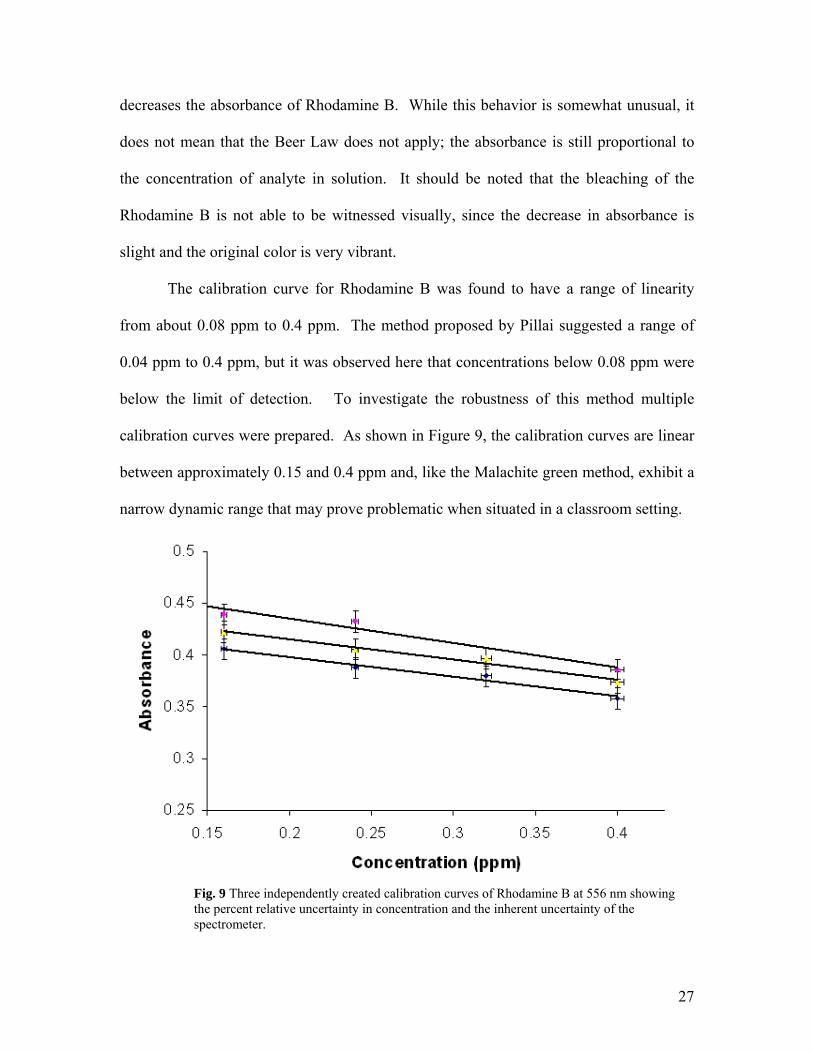
determined arsenic value that could be compared with a value obtained for one of two

different digestion methods. The sets of data were then statistically examined using a

paired t-test in order to determine whether the arsenic concentrations for each sample

were significantly different when determined by these two methods of analysis. The null

hypothesis inherent within the paired t-test is that the mean difference is zero, while the

alternative hypothesis is that the results are significantly different and that the mean

difference is greater than zero. The difference (di) between each paired value was

calculated followed by the mean difference and the standard deviation of the mean

difference. The tcalc value is equal to the following:

(│d│/ sd) * √n

If the tcalc is less than the ttable value, the null hypothesis is proved correct. If the tcalc is

greater than the ttable value, the alternative hypothesis is proved correct. In comparing the

Cherian soil digestion method with the data provided by the XRF, tcalc was calculated to

be 1.648, with a corresponding ttable value of 2.120 at the 95% confidence interval for 16

degrees of freedom. In this instance the null hypothesis was proven to be correct, and the

difference between the two data sets is NOT significant. For the EPA digestion method

3050b and the XRF data, tcalc was calculated to be 6.396 with a ttable value of 2.110 at the

95% confidence interval with 17 degrees of freedom. In this case, the alternative

hypothesis stands and the difference between the two data sets is significantly different.

These latter results are not surprising considering that the EPA method was not

able to recover much arsenic from the sample, never exceeding 25 ppm on samples which

had been analyzed using an XRF to contain over 100 ppm. This determinate error

suggests that this method is liberating other ions that can interfere with the reaction

39

pathway between either arsenic and iodate, or iodine and Rhodamine B. Either bias

would reduce the concentration for arsenic calculated for the Rhodamine B method

because less iodine would be available to react with Rhodamine B. It is also possible that

the amount of measured arsenic was reduced since the EPA method does not contain a

step that converts As (V) to As (III).

Although the abbreviated digestion scheme of Cherian was statistically

indistinguishable from the XRF results, the precision for the method was quite poor. For

example, within each triplicate data set, a range of over 50 ppm was common. Some

variation within each sample was not unexpected because the soil samples are not, of

course, entirely homogenous. Consistent with the EPA-approved procedure for soil

analysis by XRF, each sample was finely ground and passed through a fine 60-mesh

sieve (250 micron) to improve homogeneity. However, soil digestions are a bulk analysis

of the sample whereas the XRF is limited to the surface of each sample. This potential

limitation of the XRF was explored previously by analyzing aliquots taken from about

500 g of soil that had been passed through a 60-mesh sieve. The relative standard

deviations for selected ions ranged from 2-10% (Pb, 7%; Ti, 9%; Fe, 2%; Zn, 4%; Rb,

4%; and Sr, 3%). Arsenic was not included since it often falls below the limit of

detection on the XRF. Yet even by assuming a deviation of 7%, the scatter in the UV-

Vis determined results is still considerable. This is shown in Figure 17.

40

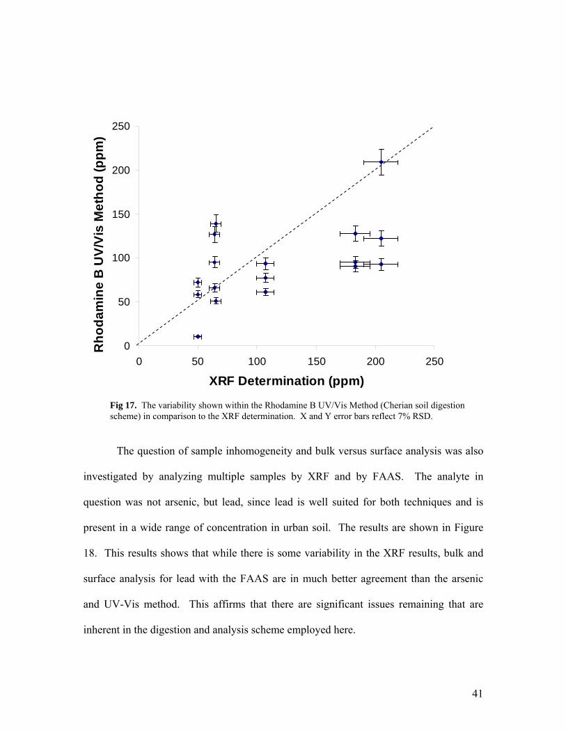
Fig 17. The variability shown within the Rhodamine B UV/Vis Method (Cherian soil digestion scheme) in comparison to the XRF determination. X and Y error bars reflect 7% RSD.

0

50

100

150

200

250

0 50 100 150 200 250

XRF Determination (ppm)

Rho

dam

ine

B U

V/Vi

s M

etho

d (p

pm)

The question of sample inhomogeneity and bulk versus surface analysis was also

investigated by analyzing multiple samples by XRF and by FAAS. The analyte in

question was not arsenic, but lead, since lead is well suited for both techniques and is

present in a wide range of concentration in urban soil. The results are shown in Figure

18. This results shows that while there is some variability in the XRF results, bulk and

surface analysis for lead with the FAAS are in much better agreement than the arsenic

and UV-Vis method. This affirms that there are significant issues remaining that are

inherent in the digestion and analysis scheme employed here.

41

Fig. 18. Comparison of bulk and surface analysis of Pb with XRF and FAAS.

3.10 – LIMITING VARIATION WITHIN CHERIAN METHOD

The Rhodamine B method is clearly capable of producing a reliable calibration

curve for arsenic determinations. However, it is not clear at all whether the Cherian

digestion procedure may be joined with the Rhodamine B method to determine the

amount of arsenic present in the soil found in Columbus, OH. To examine the digestion

procedure more closely, several different experimental parameters in the Cherian

procedure were investigated in an effort to improve the overall precision. In addition,

such an approach serves to investigate the inherent variability that will inevitably occur

should this procedure be used in an instructional setting. If one parameter in particular

did result in substantial variation, this could be a significant issue for students. Potential

sources of variability within the method alone could be caused by the color of solution

prior to adding Rhodamine B, which would affect the intensity of the peak; the amount of

42

HCl used in extraction, and the amount of time spent refluxing. The latter two could

have potential implications in the amount of arsenic brought into solution.

3.11 – DIGESTION PARAMETERS

It was observed that some soil digestion samples turned brown either after

refluxing for 30 min or the addition of potassium iodide according to the Cherian method.

This is most likely due to the formation of triiodide (Wells, 1984). The proposed reaction

is

This endergonic reaction is known to occur in the presence of dichromate and iron

cations which are common in soil. This reaction not only darkens the solution color, it

also alters the amounts of I2 available to bleach the Rhodamine B. This could potentially

attribute for the difference of concentrations measured within the three trials from a

single soil site. The reaction can be slowed by storing it in the dark and preferably in a

cool place.

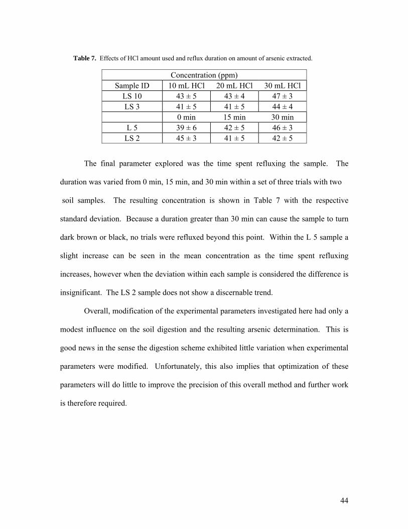
The second parameter that was explored was the amount of HCl used in the soil

digestion. It was necessary to determine whether different amounts of acid would

significantly decrease or increase the amount of arsenic extracted in order to improve the

poor precision yielded by the Cherian method. Two different soil samples were digested

in sets of three, containing 10, 20 and 30 mL of HCl. There was no other variable

introduced amongst each sample. The results are shown in Table 7. There is no

significant difference between the amounts of HCl used, considering that each value lies

within the others’ range.

43

44

Concentration (ppm) Sample ID 10 mL HCl 20 mL HCl 30 mL HCl

LS 10 43 ± 5 43 ± 4 47 ± 3 LS 3 41 ± 5 41 ± 5 44 ± 4

0 min 15 min 30 min L 5 39 ± 6 42 ± 5 46 ± 3

LS 2 45 ± 3 41 ± 5 42 ± 5

Table 7. Effects of HCl amount used and reflux duration on amount of arsenic extracted.

The final parameter explored was the time spent refluxing the sample. The

duration was varied from 0 min, 15 min, and 30 min within a set of three trials with two

soil samples. The resulting concentration is shown in Table 7 with the respective

standard deviation. Because a duration greater than 30 min can cause the sample to turn

dark brown or black, no trials were refluxed beyond this point. Within the L 5 sample a

slight increase can be seen in the mean concentration as the time spent refluxing

increases, however when the deviation within each sample is considered the difference is

insignificant. The LS 2 sample does not show a discernable trend.

Overall, modification of the experimental parameters investigated here had only a

modest influence on the soil digestion and the resulting arsenic determination. This is

good news in the sense the digestion scheme exhibited little variation when experimental

parameters were modified. Unfortunately, this also implies that optimization of these

parameters will do little to improve the precision of this overall method and further work

is therefore required.

CONCLUSIONS

There are several areas within the suggested methods of analysis that are either

problematic or contain potential problems for an undergraduate laboratory. The Leuco-

malachite green method would be a poor application in a classroom due to the narrow

dynamic range present within the calibration curve. Low concentrations are required, and

the resulting high sensitivity causes noticeable deviation. Malachite green’s sensitivity to

common ions in soil such as iron and chromium immediately rule out the method for soil

analysis since these interferrents are not able to be masked or removed from solutions.

The Rhodamine B method is more resistant to interferrents and for this reason

cannot be excluded from soil analysis like Leuco-malachite green. However, the method

has a narrow range of linearity at low concentrations which could prove problematic for

students. While the calibration curve appears to be reproducible, it would be necessary to

first test the method in a classroom and assess how robust the procedure truly is when

used by undergraduate students.

The Rhodamine B does have several logistical concerns, the most prominent

being reagent stability of less than 24 hours. This means that students would have to

complete analysis for all samples within one lab period. Since most lab periods (at OSU)

have a duration of two to four hours this may prove problematic if the sample count is

high or if mistakes are made. Additional concerns include the hazardous nature of

Rhodamine B, which is not only a soluble and strong organic dye but also a carcinogen.

Students would need to take appropriate precautions by wearing gloves and be extra

cautious in avoiding spills on skin or clothing.

45

Both of the proposed soil digestion procedures are unacceptable for application in

an undergraduate lab. Neither method was successful in quantitatively arsenic extraction.

The EPA Method 3050b appears to have a determinate error biased the arsenic analysis in

this study. This method also has a problematic time requirement that necessitates

multiple lab periods for sample digestion. In contrast, Cherian’s abbreviated method

does not include a determinate error. However, it did exhibit an unacceptably poor level

of precision and so considerable work is required before this method is suitable for

classroom use. In addition, in terms of safety considerations within the laboratory, both

of these methods require the use of concentrated acids in substantial quantities. This has

further implications due to potential space constraints since all digestions must be

completed underneath a fume hood.

In summary, the Rhodamine B method has potential for use in the UV-Vis

spectrophotometric determination of arsenic in soil samples. Logistical issues, such as

reagent stability and sample throughput, and laboratory safety concerns are not

insurmountable. Most important, however, is the need to validate a digestion procedure

capable of quantitative arsenic extraction from urban soils. With such a procedure, the

combined method would prove valuable in assessing arsenic concentration in an

inexpensive manner as well as provide a new application for UV-Vis spectroscopy in

undergraduate laboratories.

46

FUTURE WORK

This thesis provides a foundation for further work on the development of a

spectrophotometric procedure for undergraduate students aiming to determine the

concentration of arsenic in urban soils. While the Malachite green method is too

problematic for soil analysis, the Rhodamine B method still holds considerable potential.

If future research shows that Rhodamine B is not suitable for use in an undergraduate lab,

the azure B method is another possibility worth investigating. It would be most

beneficial, however to further explore a soil digestion method that fulfills the established

criteria and does not share the pitfalls of the two methods tested in this project. The EPA

has published other methods that appear promising and are based upon the same general

outline as the Cherian procedure examined here. It would be interesting to see what

further investigation along these fronts might yield.

47

48

APPENDIX A: SUGGESTED MALACHITE GREEN PROCEDURE FOR STUDENTS

MATERIALS

3M HCl 3M NaOH 2% KIO3 4 ppm Na AsO2 0.05% Leuco-malachite green Acetate buffer (pH 4.5) Previously digested soil samples Distilled water

pH 4 and pH 7 standard solutions pH meter Assorted glassware Analytical Balance Cuvettes UV-VIS Spectrometer Hot water bath

PROCEDURE:

Part A: Preparation of Stock Solutions & Calibration of pH meter

1) From the stock solutions of HCl and NaOH, prepare a 0.45M HCl solution and a second 0.45M NaOH solution in 100 mL volumetric flasks.

2) Calibrate the pH meter using the pH 4 and pH 7 standards, rinsing the probe with distilled water in between solutions. Do not dispose of the standards until the end of the lab.

Part B: Development of Calibration Curve

3) In a small beaker add 1 mL of 4 ppm NaAsO2.

4) Add 5.00 mL of 0.45M HCl and 2.50 mL of 2% KIO3 to the beaker containing the arsenic mix well for one minute.

5) Add 2.50 mL of LMG with gentle shaking, then add 10.00 mL of acetate buffer.

6) Check the pH of the solutions to make sure it falls between 4.3 and 4.7. If it is outside of this range, adjust the pH using the 0.45M NaOH or 0.45M HCl.

7) Transfer the pH adjusted solution to a 50 mL volumetric flask and bring to volume using distilled water.

8) Repeat steps 4-7 four more times choosing volumes between 2 and 15 mL of NaAsO2. There should be five flasks in total with arsenic concentrations between 0.08 and 1.2 ppm.

Part C: Preparation of Soil Samples

9) Using soil samples that were previously digested, add 1 ppm of the solution to a small beaker.

10) Add 2.50 mL of KIO3 to the beaker and mix well for one minute.

11) Check the pH of the solution in the beaker. It will be very acidic after the soil digestion. Elevate the pH using NaOH so that the ending pH is between 4 and 5. It is advisable to use 3M NaOH initially, using 0.45M NaOH when solution is close to a pH of 4.

12) Add 2.50 mL of LMG with gentle shaking, followed by 10.00 mL of acetate buffer. Ensure that the pH is now between 4.3 and 4.7.

13) Transfer the pH adjusted solution to a 50 mL flask and bring the solution to volume with distilled water. The solution should be a bluish green color.

14) Repeat steps 9-13 with each soil sample collected.

Part D: UV-VIS Analysis

15) Using distilled water as a blank, set up the spectrometer for the malachite green calibration. Take the absorbance readings at about 617 nm where the absorbance is at a maximum. Lastly, take the absorbance readings of each of the soil samples treated with LMG.

49

50

APPENDIX B: SUGGESTED RHODAMINE B PROCEDURE FOR STUDENTS

MATERIALS:

3M HCl 3M NaOH 2% KIO3 4 ppm NaAsO2 Rhodamine B Previously digested soil samples Distilled water

pH 4 and pH 7 standard solutions pH meter Assorted glassware Analytical Balance Cuvettes UV-VIS Spectrometer

PROCEDURE:

Part A: Preparation of Stock Solutions & Calibration of pH meter

1) Prepare a 0.2% solution of Rhodamine B by weighing out 0.0025 g of Rhodamine B on an analytical balance and add it to a 100 mL volumetric flask. Bring to volume with distilled water and mix well.

2) From the stock solutions of HCl and NaOH, prepare a 0.45M HCl solution and a second 0.45M NaOH solution in 100 mL volumetric flasks.

3) Calibrate the pH meter using the pH 4 and pH 7 standards, rinsing the probe with distilled water in between solutions. Do not dispose of the standards until the end of the lab.

Part B: Development of Calibration Curve

4) In a small beaker add 1 mL of 4 ppm NaAsO2.

5) Add 2.00 mL of 0.45M HCl and 2.00 mL of 2% KIO3 to the beaker containing the arsenic mix well for one minute.

6) Check the pH of the solutions to make sure it falls between 4.5 and 8.5. If it is outside of this range, adjust the pH using the 0.45M NaOH or 0.45M HCl.

7) Transfer the pH adjusted solution to a 50 mL volumetric flask. Add 2.00 mL of 0.2% Rhodamine B, mix well, and bring to volume using distilled water.

8) Repeat steps 4-7 with 2, 3, 4, and 5 mL of NaAsO2. There should be five flasks in total with arsenic concentrations of 0.08, 0.16, 0.24, 0.32, and 0.40 ppm.

Part C: Preparation of Soil Samples

9) Using soil samples that were previously digested, add 1 ppm of the solution to a small beaker.

10) Add 2.00 mL of KIO3 to the beaker and mix well for one minute.

11) Check the pH of the solution in the beaker. It will be very acidic after the soil digestion. Elevate the pH using NaOH so that the ending pH is between 4.5 and 8.5. It is advisable to use 3M NaOH.

12) Transfer the pH adjusted solution to a 50 mL flask and add 2.00 mL of 0.2% Rhodamine B. Bring the solution to volume with distilled water. The solution should be a vibrant pink color. If the solution appears violet or orange, check the pH once more to ensure that it is within the proper range. If a precipitate is present, the solution may need to be within the high end of the pH range, around 8 or 8.5.

13) Repeat steps 9-12 with each soil sample collected.

Part D: UV-VIS Analysis

14) Using distilled water as a blank, set up the spectrometer for the Rhodamine B calibration. Take the absorbance readings at about 556 nm where the absorbance is at a maximum. Lastly, take the absorbance readings of each of the soil samples treated with Rhodamine B.

51

52

APPENDIX C: SUGGESTED CHERIAN SOIL DIGESTION PROCEDURE FOR STUDENTS

MATERIALS:

Finely ground soil samples Conc. HCl 10% KI Ascorbic Acid Distilled Water

Hot plate Analytical Balance Whatman Filter Paper Glass Funnel Assorted Glassware

PROCEDURE:

Part A: HCl Extraction

1) Weigh out approximately 1 g of soil that has been finely ground and sieved into a 100 mL beaker.

2) Under a hood, slowly add 5.0 mL of concentrated HCl. Wait several minutes for the reaction to occur with occasional swirling; there may be some fizzing and gas produced.

3) Pour off the liquid into the funnel containing the filter paper, collecting the liquid in a beaker.

4) Repeat steps 2 and 3 two more times.

5) With a final 5.0 mL portion of HCl, rinse the remaining soil in the beaker and the filter paper.

6) Reflux the HCl extract on a hot plate for about 30 min. If the extract begins to turn chocolate brown or black after refluxing for only 20 min or so, remove it from the heat source. Allow the solution to cool to room temperature.

Part B: Treatment of Digestion Extract

7) Transfer the extract to a 50 mL volumetric flask that contains 15 mL of distilled water.

8) Add 10% KI dropwise to reduce any arsenic (V) to arsenic (III) until the presence of excess iodine is seen. This is evidenced by a reddish brown color. This requires about 5-15 drops.

9) Add 1 mL of ascorbic acid to destroy the excess iodine. Continue to add in 1 mL portions until the reddish brown color caused by the iodine disappears.

10) Bring the solution in the flask to volume with distilled water.

NOTE: After adding KI the solutions must be kept in a cool, dark place. If it will be several days before the solutions are used for testing, it may be best to stop after completing step 7, and finishing 8-10 on the day analysis is performed.

APPENDIX D: SUGGESTED SOIL DIGESTION PROCEDURE FOR STUDENTS (EPA 3050B)

MATERIALS

Finely ground soil samples Conc. HCl Conc. HNO3 30% H2O2 Assorted glassware

Hot Plate Glass funnel Whatman Filter Paper Analytical Balance Distilled Water

PROCEDURE:

1) Weigh out approximately 1 g of a finely ground and sieved soil sample into a 100 mL beaker.

2) Under a hood, add 10 mL of concentrated HNO3 to the beaker. Cover with a watch glass and reflux for 10-15 min. Allow the sample to cool.

3) Add an additional 5 mL of concentrated HNO3, replace the cover, and reflux for 30 min.

4) If brown fumes are generated in step 3, repeat step 3 over and over until no brown fumes are seen. Reflux for two additional hours. Allow sample to cool.

5) To cooled sample, add 2 mL H2O and 3 mL of 30% H2O2. Cover the solution with a watch glass and warm the solution until effervescence ceases. If effervescence becomes vigorous, reduce the temperature.

6) Continue to add 1 mL of 30% H2O2 with warming until the effervescence ceases or becomes minimal following the addition. Do not add more than a total of 10 mL of H2O2. Reflux for an additional two hours. Allow solution to cool.

7) To a cooled solution, add 10 mL of concentrated HCl and reflux for an additional 15 minutes. Cool to room temperature.

8) Filter cooled solutions using gravity filtration into a 100 mL volumetric flask. Bring to volume using distilled water.

53

REFERENCES Alvarez-Benedi, J., Boado, S., Cancillo, I., Calvo, C., and Garcia-Sinovas, D., (2005). Adsorption-desorption of arsenate in three Spanish soils. Vadose Zone Journal, 4, 282-290. Brady, J.E. and Senese, F. Chemistry: Matter and its Changes (5th edition). John Wiley & Sons, 2009. Brown, T.L., LeMay Jr,, H.E., Bursten, B.E. Chemistry: The Central Science (10th edition). Pearson Prentice Hall. 2006. Burdge, J. Chemistry. McGraw-Hill, 2009. Casey, J., and Tatz, R. Absorbance Spectra, General Chemistry Laboratory Experiments Vol. 3, Hayden-McNeil Publishing, 1997. Chen, M., Ma, L.Q., Hoogeweg, C.G., and Harris, W.G. (2001). Arsenic background concentrations in Florida, U.S.A. surface soils: Determination and interpretation. Environmental Forensics, 2, 117-126. Cherian, T., Narayana, B. (2005). A new spectrophotometric method for the determination of arsenic in environmental and biological samples. Analytical Letters 38, 2207-2216. Chirenje, T., Ma, L., Clark, C., and Reeves, M. (2003). Cu, Cr and As distribution in soils adjacent to pressure-treated decks, fences and poles. Environmental Pollution, 124, 407-417. Craul, P.J. (1985). A description of urban soils and their desired characteristics. J. Arboriculture, 11, 330-339. De Gregori, I., Fuentes, E., Olivares, D., and Pinochet, H. (2004). Extractable copper, arsenic and antimony by EDTA solution from agricultural Chilean soils and its transfer to alfalfa plants. Journal of Environmental Monitoring, 6, 38-47. EPA Method 3050B: Acid digestion of sediments, sludges, and soils. EPA Method 3051: Microwave assisted acid digestion of sediments, sludges, soils, and oils. Grannas, A.M. and Lagalante, A.F. (2010). So these numbers really mean something? A role playing scenario-based approach to the undergraduate instrumental laboratory. J. Chem. Ed. 87(4), 416-4-18. Holleman, A. F.; Wiberg, E. (2001). Inorganic Chemistry. San Diego: Academic Press.

54

55

Mandal, B.K., and Suzuki, K.T. (2002). Arsenic round the world: A review. Talanta, 58, 201-235. Masterton, W.L., and Hurley, C.N. Chemistry: Principles and Reactions (6th edition). Brooks/Cole 2009. Mattschullat, J. (2000). Arsenic in the geosphere- A review. Sci. Total. Environ. 249, 297-312. Muyskens, M. A., and Sevy, E.T. (1997). The remarkable resilience of Beer’s Law. J. Chem. Ed. 74(9), 1138. Petrucci, R.H., Harwood, W.S., Herring, F.G., and Madura, J.D., General Chemistry: Principles and Applications (9th edition). Pearson Prentice Hall. 2007. Pillai, A., Sunita, G., and Gupta, V.K. (2000) A new system for the spectrophotometric determination of arsenic in environmental and biological samples. Analytica Chimica Acta 408, 111-115. Quaghebeur, M., Rate, A., Rengel, Z., and Hinz., C. (2005). Heavy metals in the environment. Desorption kinetics of arsenate from Kaolinite as influenced by pH. J. Environ. Qual. 34, 479-486. Revanasiddappa, H.D., Dayananda B.P., Kumar T.N.K. (2007) A sensitive spectrophotometric method for the determination of arsenic in environmental samples. Environ. Chem. Letters 5, 151-155. Silberberg, M.S. Chemistry: The Molecular Nature of Matter and Change (5th edition). McGraw-Hill, 2006. Skoog, D.A., Holler, F.J., and Nieman, T.A. Principles of Instrumental Analysis (Fifth Edition). Brooks/Cole, 1998. Suding, H.L. and Buccigross, J.M. (1994). A simple lab activity to teach subtractive color and Beer’s Law. J. Chem. Ed. 71(9), 798-799. Tro, N.J. Chemistry: A Molecular Approach. Pearson Prentice Hall. 2007. Wells, A.F., Structural Inorganic Chemistry, Oxford: Clarendon Press, 1984. Zumdahl, S.S. and Zundahl, S.A. Chemistry (7th edition). Houghton Miflin, 2009.