Investigating the Impact of Tollson High-Occupancy-Vehicle LanesUsing Managed Lanes

Mark W. Burris, David H. Ungemah, Maneesh Mahlawat,and Mandeep Singh Pannu

For nearly 40 years, high-occupancy-vehicle (HOV) lanes have beenused to combat congestion. These lanes allow only vehicles with multipleoccupants and generally offer a free-flow trip, unlike adjacent generalpurpose lanes. In theory, this encourages additional carpooling, reducesoverall vehicle miles of travel, and improves the commute trip. However,as a result of the underutilization of some of these lanes, some HOVlanes are migrating to high-occupancy-toll (HOT) lanes, where HOVsmay travel free of charge but lower-occupancy vehicles can pay a toll touse the lane. This research investigated the impacts of offering preferen­tial treatment for HOVs on these lanes. To determine the impact of dif­ferent HOT lane operating strategies on their travel behavior, freewaytravelers in the Houston and Dallas metropolitan areas ofTexas were sur­veyed. A nested logitmodel was developed to estimate the mode choice fortravelers. This model was used to predict the impact of converting anHOV lane to a HOT lane on which all travelers pay a toll. It was foundthat the overall percentage of HOV2 and HOV3+ vehicles in the trafficstream decreased by only a small amount when a toll was required forthem to use the HOV lane. However, that decrease did represent a signifi­cant portion of those modes (more than 9%) and resulted in more than a10% increase in HOT lane revenue. Therefore, elimination of preferen­tial treatment for these vehicle types has significant implications andbecomes a difficult policy decision-not just a straightforward choice.

The concept of tolling on managed lanes (MLs) has evolved sincethe first iterations in the early 1990s. Initially conceived as the per­mission for previously prohibited vehicles to use high-occupancy­vehicle (HOV) lanes in exchange for the payment ofa fee, otherwiseknown as high occupancy toll (HOT) lanes, managed lanes haveexpanded in scope to include a variety of implementations, gener­ally called express toll lanes (BTL), and are without any inherentpolicy concerning HOVs.

HOV lanes have a longer history ofoperation in North America thanHOT lanes and ETL facilities. First implemented on Virginia's Shirley

M. W. Burris, CE/lT1 Building Room 301G, and M. S. Pannu, CE/TTI BuildingRoom 3031, Zachry Department of Civil Engineering, Texas A&M University,3136 TAMU, College Station, TX 77843-3136. D. H. Ungemah, Austin Office,Texas Transportation Institute, Texas A&M University System, 1106 ClaytonLane, Suite 300E, Austin, TX 78723. M. Mahlawat, Baez Consulting, LLC, 4925Greenville Avenue, Suite 1300, Dallas, TX 75206. Corresponding author: M. W.Burris, mburris@tamu.edu.

Transportation Research Record: Journal of the Transportation Research Board,No. 2099, Transportation Research Board of the National Academies, Washington,D.C., 2009, pp. 113-122.001: 10.3141/2099-13

113

Highway busway facility (1-395) in 1969, HOV lanes provided anincentive to carpool or vanpool. Although the magnitude oftravel-timesavings offered by HOV lanes has been studied, the role ofHOV-lane­related incentives relative to other incentives to carpool has rarelyreceived the same attention. Nationally, since 1993, vehicle nules trav­eled have increased by 25%, while the percentage use and absolutenumber of carpools and vanpools for commute trips has declined to a30-year low: 10,057,000 trips in 2003, down from 11,852,000 in 1993(1). In nearly the same 10-year time frame, HOV lane miles have morethan doubled, from approximately 1,300 lane miles in 1995 to morethan 2,500 in 2000 and 3,100 in 2005. The majority ofthese HOV lanemiles are located in California (1,000), Georgia (400), and Texas (300)(2). In the HOV corridors, carpooling rates have increased significantly(more than 100%) even as carpool rates nationwide have declined(30%) during the past two decades (3). However, severe congestion inthe general purpose lanes has tended to cause animosity on the part ofthe general public toward HOV lanes if they are underutilized (3). Asa means of mitigating the "empty lane syndronle," HOT lanes havebeen promoted as an effective way of utilizing the excess capacitywithout reducing the HOV lanes' travel~time advantages (4).

In addition to HOT lanes, which imply maintenance of HOV oper­ations, ETL concepts have also been promoted as a means ofenhanc­ing mobility in congested corridors and regions. First implemented inOrange County, California, as the privately built and operated StateRoute 91 (SR-91) express toll corridor, BTL facilities provide thesame benefits ofHOT lanes (exclusive tight-of-way with congestion­free trips along the length of the corridor), but they did not originallycarry the same implied benefit to carpools and vanpools. During its10 years ofoperation, the SR-91 express toll facility has, at times, pro­vided free use by three-people-or-more (HOV-3+) carpools, but atother times required partial toll payment by these users. AlthoughSR-91 is the only ETL facility currently ill; operation, BTL conceptsmay be increasingly attractive for those' transportation agenciesseeking enhanced sources of revenue and ease of enforcement.

As managed lanes are considered throughout more than 25 NorthAmerican cities, there is a need for research and guidance defining therole of carpools in ETLs and the trade-offs between carpool exemp­tions and other project objectives. Increasingly, project objectives arereflecting not only mobility concerns but also funding deficiencies andthe need to generate revenue. As a result, allowing discounted-toll ortoll-exempt users such as carpools requires an evaluation of revenueimpacts as well as mobility interests.

The Texas Department ofTransportation commissioned the TexasTransportation Institute and University ofTexas at Arlington to studythe proper role of incentives to carpoolers in managed lane facilities.Using more than 4,600 responses to an adaptive stated-preference

114

survey of regional travelers in Dallas and Houston, the researchteam developed a model for examining the core question of the com­missioned research: what are the benefits and drawbacks of providingcarpools with discounted or toll-free use of managed lane facilities?This paper describes the survey's data collection methodology andspecialized weighting methodology used to analyze the core researchquestion.

LITERATURE REVIEW

HOY lanes and carpooling have an overlapping purpose: encouragegreater person throughput through greater vehicle occupancies. Byencouraging people to rideshare, particularly during peak periods,person throughput on congested corridors can increase without acorresponding significant increase in capacity. Since 1969 HOY laneshave been implemented with the explicit purpose ofencouraging theformation of new carpools and enhancing the performance of transitthrough a significant, reliable travel time incentive.

Although distinction is made between regular carpools (recurring,scheduled carpools) and occasional carpools (situational carpoolsonly), the basics of carpooling on HOY lanes has remained the samefor 35 years-a minimum of two or three people with common com­mute patterns share one vehicle for their trip on an exclusive facility.Carpooling itself requires no public investment because the decisionto carpool remains a private one. However, advocates for govern­mental and commercial encouragements to carpool rationalize that"every person added to a carpool means another congestion- andpollution-causing car is taken off the road" (5). As practice holds, ifcommuters are presented with a large enough incentive to switchfrom driving alone to carpooling, they may form a carpool either for­mally (through a matching service or agreement) or causally (throughsituational agreement). Travel time savings from HOY lanes haveconstituted a large portion of that incentive.

Studies have shown that there are three main reasons com­muters switch from driving alone to ridesharing (either carpoolsor vanpools):

• Travel time. Research has shown that commuters are likely toalter their commute choice if it reduces their commute time. Becausedriving alone is typically the quickest means from home to work(or the reverse), total travel time is one factor that makes drivingalone attractive to drivers (6-9). HOY lanes have been shown toreduce travel time, thereby making carpooling more appealing andcounteracting the disposition toward driving alone (9-11).

• Convenience. Studies have also confirmed that convenience is afactor in determining mode choice. Driving alone is seen as the mostconvenient mode for most commuters. However, this can change ifemployers or municipalities have carpooling incentives in place mak­ing carpooling more suitable for their needs, such as convenientlylocated parking spaces reserved for carpoolers (6-8, 12, 13).

• Cost. Although many commuters do not use the most cost­effective commute choice, it is an influential factor. Cost savings canbe realized simply through the sharing of costs between driver andpassenger(s), although additional financial incentives and subsidiesmay be offered by governmental or employer entities or both. Thisis true especially with vanpool programs (9, 12, 13). Researchersnote that free or low-cost parking tends to influence a greater use ofsingle-occupant vehicles (12).

Benefits from carpooling, which HOY lanes endeavor to encour­age, can be articulated for users and society. User benefits include

Transportation Research Record 2099

personal cost savings and perceived quality of life enhancements.Many commuters underestimate the true cost of driving alone to andfrom work. The cost of commuting may be significantly reducedwhen carpoolers or vanpoolers share the costs. This is true especiallyin situations with added costs, such as parking fees and tolls, in addi­tion to fuel (14,15). Commutes are increasingly becoming too con­gested and stressful, which can be carried over into professional andsocial situations. Carpooling enables riders to relax and allows themto arrive at their destination without the stress of driving (14, 16).

Societal benefits are most typically associated with reduction invehicular use (and corresponding reduction in vehicle miles traveled)and a resulting improvement in air quality. In areas of serious air qual­ity concerns, carpooling and HOY lanes together constitute importantelements in achieving conformity with air quality targets (17). Cou­pled with the perception of HOY lanes and carpooling as enablingbroader environmental objectives (including favorable land use andfuel consumption goals), a significant stakeholder community hasformed around their continued use and promotion.

However, further investigation into current carpooling trends indi­cates that the majority of carpools are family oriented, a type of car­pooling called "fampools" (18). Only 26% of surveyed travelers inHouston in 2001 taking a work tour carpool involved a non-householdmember, compared with 74% involving a family member (19). Criticshave argued that the extensive amount of household-member-onlycarpooling for work trips belies the premise behind the investment inHOY lanes-that it will encourage the formation ofcarpools betweentwo drivers, explicitly to take advantage of the travel time savings inthe HOY lanes (18).

That fampooling does not take cars off the street is evident partic­ularly when HOY lanes are used by drivers whose passenger is some­one who, for a variety of reasons, would not be driving anyhow. Forexample, it is certainly convenient for a parent driving with a son ordaughter to use the carpool lane, but as long as the son or daughter isunder the legal driving age, this sort ofcarpool does not spare the roadfrom an extra car (18).

Fampooling criticism implies that family members who carpoolwould do so with or without the presence of HOY lanes and otherincentives. However, a counterargument suggests that familial car­pools (particularly involving two or more adults) are perfectly legit­imate to the extent that those family members would otherwise driveseparately.

With the decline in HOY travel in general (but an increase inHOY travel in areas with HOY lanes), the significant presence offampools, the need to maximize the use of existing infrastructure,and transportation funding shortfalls, it is imperative that the bene­fits and disbenefits of providing preferential treatment for carpoolson exclusive facilities (such as ETLs) be examined.

DATA COLLECTION

To better estimate the potential impacts ofeliminating or reducing thepreferential treatment of HaYs on HOY lanes, a survey of travelerswas undertaken. The survey was performed in two Texas metropoli­tan areas (Houston and Dallas) that have high levels ofcongestion andnumerous HOY lanes. The survey focused on people who regularlytraveled on one or more of those cities' major roadways. A list of31 major roadways and tollways in the two cities, including all thosewith HOY lanes, was developed for use in the survey. Thus, manyof the respondents already traveled on a roadway with a toll or anHOY lane, and the rest traveled on roadways on which an HOY,HOT, or managed lane might be added at a future date.

Burris, Ungemah, Mahlawat, and Pannu

The survey was administered via the Internet in both English andSpanish from May to July 2006. Many Houston and Dallas trans­portation organizations helped in announcing and providing Internetlinks to the survey. A couple of local news stations also announcedthe survey, helping to generate 4,280 responses via the Internet. Addi­tional survey efforts were required because those 4,280 respondentsdid not accurately reflect the socioeconomic characteristics of peoplein Houston and Dallas. Survey crews administered paper-and laptop­based surveys at community centers and driver's license offices inlow-income and minority neighborhoods. This effort garnered anadditional 354 surveys, many from underrepresented groups. Unfor­tunately, the 4,634 total respondents still did not reflect the ethnicand economic makeup ofthe two cities, so a weighting process wasundertaken (see the next section).

115

used to calculate replicate weights begins with dividing the sampleinto subsamples. The same 16 subsamples or strata (per city) wereused with the replicate weights as were developed for the pweights.Next, the estimate of interest is calculated from the subsample andthe full sample. The difference between the estimates of interest inthe full sample and each of the subsamples is used to determine thestandard error of the estimate.

For example, assume Sis the full-sample estimate of some popu­lation parameter S, for example, the mean. The variance estimationQ"2(f) is given by

(2)

where hg is the factor specific to JK-n methodology and/g is the finitepopulation correction factor.

The finite population correction factor (/g) is estimated usingEquation 4 (21). In both Houston and Dallas this value was extremelyclose to 1.

where

8g = estimate of S based on the observations included in the gthreplicate (subsample);

G = total number of subsamples (or replicates formed);c = constant depending on the replication method (20); for Jack­

knife-n, C = 1; andg = replicate number.

Different methods ofcreating subsamples yield different kinds ofreplicate weights. Because this survey of ML travelers had morethan two primary sampling units per stratum (Houston road, Dallasroad, neither of the given roads in Houston or Dallas, or missinglocation), the Jackknife-n (JK-n) method was the only appropriatemethod. For the JK-n method, the formula for variance estimationis modified as shown in Equation 3.

SURVEY DATA ANALYSIS

Replicate Weighting Process

The sampling design for this survey of ML travelers was simple ran­dom sampling (SRS) followed by poststratification. Because of thisdata collection method, the statistical formulas and methods developedfor survey analyses on SRS data were inappropriate. SRS would implythat for each stratum, the proportion of respondents in the sample wasthe same as the proportion in the population. The sample proportionsfor this survey were not equal to population proportions for eachstratum, necessitating a weighting process using replicate weights.

In SRS, the sampling weights are fixed depending on the propor­tions ofeach stratum in the population. Ifthe sampling plan is not SRS,the sampling weights (pweights) developed poststratification dependon the given sample size. In other words, the sampling weights are ran­dom. They cannot be used like fixed weights to conduct tests of pro­portions or for testing other hypotheses. The reason is that a non-SRSmethodology results in higher standard errors (SEs) for the estimates.An assumption of fixed weights (with SRS) would imply lower SE.Thus, using fixed weights may lead to some results from non-SRSsurveys being found statistically significant when in fact they are not.

To address that issue, replicate weights were calculated using post­stratification weights as the input. Income (four groups), ethnicity(four groups), and toll-road use (two groups) were used as the criteriafor computing the poststratification weights (pweight). The formulafor the pweight calculation is FPC = [(N -n)/(N -I)t

(3)

(4)

% poppweight= I

% sample;(I)

where N is total population and n is total sample size.The number of replicates, G, is equal to

where

% pop; = percentage of population in stratum i,% sample; = percentage in survey sample in stratum i, and

stratum; = group (or stratum) of the survey.

For example, one stratum could be Caucasians with annual house­hold incomes less than $25,000 who traveled on a toll road.

The poststratification weights for the survey were computed usingan iterative procedure. The final pweights were used to adjust thesurvey sample from each city (Houston and Dallas) to match thatcity's population (based on the 2005 American Community Surveydata and average annual daily traffic volumes) in all 16 strata (fourincome groups by four ethnic groups).

Next, replicate weights were used to calculate a better approxima­tion of the standard error of the full sample estimates. The method

(5)

where L equals number of strata (16 in this case) andnh (varies from2 to 4) equals number ofprimary sampling units in stratum h. G totaled39 for this survey.

The methodology for replicate weight creation is given in detailin WesVar Manual (21): "For computation of first replicateweight, the full sample of observations in the first stratum andfirst primary sampling unit (PSU) are given a weight of zero andthe weights associated with the other PSU in the same stratum areadjusted by

116

[in this case often 2] to account for reducing the sample. The weightsfor observations in all the other strata are not changed. The remain­ing replicates for the stratum (weights and 8g) are formed in the samemanner by systematically dropping each ofthe remaining PSUs forthat stratum and computing the replicate weights in a manner simi­lar to computation of the first replicate weight." Then each stratumis done in a similar manner.

Descriptive Analysis of the Data

Next, descriptive statistics were developed using the replicate weightsand the fixed (or P) weights. This information was used to help deter­mine what variables would most likely be included in the mode choicemodel (discussed below) and to provide some insight into the impactof using replicate weights. The analysis divided the sample into twogroups: (a) respondents who selected a managed lane option in atleast one of the four stated preference questions (approximately71 % of respondents) and (b) respondents who never chose an MLoption. The results ofthis analysis are provided in Table 1. Significantp-values indicate that respondents with that characteristic selectedan ML option significantly more or less than respondents with theother characteristics. For example, travelers with a trip purpose of"other" were significantly less likely to choose an ML option thanall other travelers combined.

As shown in Table 1, the means calculated using the replicate andfixed weights are the same; it is the standard deviations that change.In general, the standard deviations calculated by the replicate weight­ing method were larger, and therefore the probability (p-values) wasalso larger, indicating a lower likelihood that the differences observedwere statistically significant. In the categories listed in Table 1,13 were found to be significantly different using P weights, but thecorrect method, using replicate weights, found only six significantdifferences. The differences were not surprising, and respondentsmore likely to choose an ML option:

• Were not on a trip purpose categorized as "other,"• Were younger than 65 years old,• Were traveling on a Dallas toll road,• Had one vehicle per household, and• Had a household income between $25,000 and $49,999 or greater

than $100,000.

Mode Choice Model Development

A mode choice model based on respondents' answers to the statedpreference questions was then developed. All six mode options wereavailable in the model:

• Single-occupant vehicle (SOV) on the managed lanes (MLs),• Two-person vehicle (HOV2) on the MLs,• Three-or-more-person vehicle (HOV3+) on the MLs,• SOY on the general purpose lanes (GPLs),• HOV2 on the GPLs, and• HOV3+ on the GPLs.

Although transit was available in many ofthese corridors, it was notincluded as a mode choice. It was felt that an additional mode wouldadd too much complexity to the choice set, and previous researchshowed transit riders to be loyal to the bus mode (19).

Transportation Research Record 2099

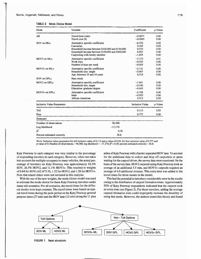
Nested and random parameter logit models were estimated for modechoice modeling using the maximum likelihood method in LIMDEP.Several utility equations with varied combinations of parameters wereexamined. The utility function of the nested logit model shown inTable 2 was found to have best fit and explanatory ability. The nest isshown in Figure 1. One side of the nest contains respondents whochose a toll option, including SOY on the MLs and most of the HOV2son the ML. The other side of the nest includes non-toll-paying travel­ers on the GPLs and most ofthe HOV3+ travelers on the MLs. Becauseof the random features built into the stated preference questions, 1,078stated preference questions of 17,176 included HOV2s who paid notoll on the ML or HOV3+ travelers who paid a toll on the ML. Thesewere removed before model estimation for this nest. Driving alone onthe GPLs was taken to be the base mode.

All variables used in the model were significant at the 95% con­fidence level (see Table 2). Apart from its statistical significance,each variable in the model was examined for its sign and magnitude.All parameters used in the model seemed reasonable on the basis ofthe literature review and the survey descriptive statistics. For exam­ple, work-related trips and adults living alone were less likely to car­pool. Conversely, Caucasians with high incomes were more likelyto use the MLs as an SOY, whereas fampools were much less likelyto break up and use the ML as an SOY. From the model, the value oftime for travelers was found to be $12.60 per hour. This value seemsreasonable as compared with other studies and national guidance, inwhich the value generally is in the $15/h range.

HOV LANE VERSUS MANAGEDLANE SIMULATION

This survey of travelers and the mode choice model developed inthe previous section were designed to better understand the impactof preferential treatment for carpoolers on managed lanes. This sec­tion of the paper presents one-example of how these data may beused to accomplish that objective. In this section, the mode choicemodel was applied to Katy Freeway automobile travelers, and theirmode choices due to varying toll levels were investigated.

Katy Freeway Travelers as the Test Group

Katy Freeway was chosen as an example corridor to use in this sim­ulation because this freeway already has an HOV lane and many ofthe travelers along the freeway already carpool. This provided a sig­nificant number of carpool respondents (130) of the many total sur­vey respondents (498) who regularly traveled that freeway. This highpercentage of carpoolers was us.eful when the model was applied. Ifthe percentage of carpoolers was too small, the model may not haveproperly estimated the impact oftolls and travel times on this group'smode choice.

However, to simulate the impact of preferential toll treatment oncarpoolers on Katy Freeway another set of weights was developed.These weights adjusted the average weights by the ratio of surveyedto actual SOV, HOV2, and HOV3+ travelers on the Katy corridor dur­ing the 3-h peak period. Survey respondents who traveled by auto­mobile on the Katy Freeway were primarily in SOVs (73.9%),followed by HOV2 carpools (17.5%), and then HOV3+ carpools(8.6%). Actual percentages of these groups on Katy Freeway wereobtained from average vehicle occupancy counts on the main lanes,frontage roads, and HOV lane. The actual percentage of vehicles on

Burris, Ungemah, Mahlawat, and Pannu

TABLE 1 Descriptive Stetistics of Survey Respondents

Replicate Weights PWeightsCharacteristic N Choose ML (%) p-Value (%) Choose ML (%) p-Value (%)

Trip Purpose

Commute 2,364 71.6 0.40 71.6 0.40

Recreational 651 74.8 0.26 74.8 0.18

Work-related 582 69.4 0.33 69.4 0.30

School 154 77.0 0.31 77.0 0.29

Other" 93 52.5 O.Ola 52.5 O.04a

Road

Houston: Beltway 8 (only Houstontoll road in list) 106 79.3 0.13 79.3 0.03a

Houston: all other roads listed 2,178 72.2 0.35 72.2 0.32

Dallas: George Bush Turnpikeand Dallas North Tollway(only Dallas toll roads in list) 219 80.0 0.00" 80.0 0.00"

Dallas: all other roads listed 1,203 67.1 0.10 67.1 O.Ola

No road selected 182 78.7 0.22 78.7 0.16

Time of Travel (multiple answers allowed)

Early a.m. (midnight-6 a.m.) 513 68.8 0.29 68.8 0.26

Peak a.m. (6 a.m.-9 a.m.) 2,190 72.1 0.37 72.1 0.36

Midday (9 a.m.--4 p.m.) 1,080 71.9 0.40 71.9 0.40

Peak p.m. (4 p.m.-6:30 p.m.) 1,929 73.2 0.24 73.2 0.16

Late p.m. (6:30 p.m.-midnight) 649 74.4 0.29 74.4 0.23

Typical Trip Length

Short (0-3 miles) 140 65.4 0.31 65.4 0.24

Medium (4--9 miles) 582 70.4 0.38 70.4 0.34

Long (10-20 miles) 1,736 72.1 0.39 72.1 0.38

Very long (more than 21 miles) 1,206 72.7 0.37 72.7 0.34

Pay to Park at Destination

Yes 599 68.1 0.26 68.1 0.17

No 3,266 72.4 0.26 72.4 0.17

Number of People in the Vehicle

One 2,374 70.5 0.27 70.5 0.20

Two 515 76.3 0.20 76.3 0.08

Three or more 239 77.1 0.30 77.1 0.19

Vanpool, train, bus, or motorcycle 572 69.2 0.26 69.2 0.29

Number of Trips per Week

lor2 311 72.7 0.40 72.7 0.39

3 to 5 1,183 72.1 0.40 72.1 0.40

6t09 490 68.4 0.32 68.4 0.25

10 1,205 72.5 0.38 72.5 0.37

More than 10 568 72.8 0.39 72.8 0.38

Travel Companion (only for carpoolers)

Coworker (nearby office) 164 78.4 0.39 78.4 0.37

Adult family member 338 72.9 0.24 72.9 0.13

Child 136 78.8 0.38 78.8 0.37

Other 87 86.1 0.12 86.1 0.11

(continued on next pagel

117

,I118 Transportation Research Record 2099

! I, I TABLE 1 (continued] Descriptive Statistics of Survey Respondents

Replicate Weights PWeightsCharacteristic N Choose ML (%) p-Value (%) Choose ML (%) p-Value (%)

Age

16 to 24 years old 481 79.9 0.12 79.9 0.02a

25 to 34 years old 1,280 75.1 0.15 75.1 0.05a

35 to 44 years old 914 72.4 0.39 72.4 0.38

45 to 54 years old 784 64.6 0.06 64.6 0.00-

55 to 64 years old 361 68.8 0.33 68.8 0.25

More than 65 years olda 94 50.5 O.03a 50.5 0.00-

Gender

Male 2,033 73.0 0.24 73.0 0.18

Female 1,873 70.0 0.24 70.0 0.18

Ethnicity

Caucasian 1,908 73.6 0.18 73.6 0.10

Afro-American 602 72.7 0.39 72.7 0.37

Hispanic 860 71.1 0.40 71.1 0.39

Other 556 64.9 0.08 64.9 0.09

Household Type

Single adult 1,160 70.9 0.39 70.9 0.37

Unrelated adults (e.g., roommates) 273 79.5 0.15 79.5 0.07

Married without child 704 73.9 0.28 73.9 0.21

Married with child(ren) 1,270 71.3 0.40 71.3 0.39

Other 468 66.0 0.14 66.0 0.13

Household Size

One 776 66.8 0.10 66.8 O.04a

Two 1,169 73.2 0.33 73.2 0.30

Three 695 72.4 0.39 72.4 0.39

Four 652 75.0 0.20 75.0 0.18

Five or more 447 72.7 0.39 72.7 0.39

Number of Vehicles

None 41 65.8 0.35 65.8 0.38

One 1,097 67.2 0.03a 67.2 0.02a

Two 1,692 74.0 0.19 74.0 0.09

Three or more 986 73.6 0.30 73.6 0.26

Occupation

Professional 1,624 71.8 0.40 71.8 0.39

Technical 469 70.4 0.37 70.4 0.37

Administrative 602 68.7 0.31 68.7 0.24

Sales, service, manufacturing,student, and self-employed 755 76.7 0.10 76.7 0.05a

Stay-home, unemployed,retired, and others 403 67.4 0.30 67.4 0.22

Education

High school graduate or less 654 69.5 0.31 69.5 0.31

Some college, vocational 1,245 70.5 0.34 70.5 0.33

College graduate 1,337 74.0 0.18 74.0 0.10

Postgraduate degree 675 70.9 0.39 70.9 0.38

Income

Less than $24,999 978 74.3 0.18 74.4 0.23

$25,000 to $49,999 1,099 66.4 O.01 a 66.4 0.01"

$50,000 to $99,999 1150 71.7 0.40 71.7 0.40

More than $100,000- 700 76.0 O.01 a 76.0 O.Ola

aStatistically significant at 95%.

Burris, Ungemah, Mahlawat, and Pannu

TABLE 2 Mode Choice Model

119

Mode

All

SOVonMLs

HOV20nMLs

HOV3+on MLs

SOVonGPLs

HOV20nGPLs

HOV3+ on GPLs

Inclusive Value Parameters

Toll

Free

Summary

Number of observations

Log likelihoodp2Percent estimated correctly

Variable

Travel time (min)Travel cost ($)

Alternative specific coefficientCaucasianHousehold income between $100,000 and $150,000Household income between $150,000 and $200,000Carpooling with family member

Alternative specific coefficientWork tripsNumber of trips per week

Alternative specific coefficientHousehold size: singleAge: between 35 and 44 years

Base mode

Alternative specific coefficientHousehold size: singleEducation: graduate degree

Alternative specific coefficientMaleAfrican American

96,588

-17,170

0.30

36.8

Coefficient

-0.0077-0.0365

-6.5700.1650.3330.907

-1.655

-7.173-0.533-0.055

-2.131-0.907

0.518

-1.841-0.450-0.443

-2.728-0.953

0.312

Inclusive Value

0.113

0.777

p-Value

0.000.00

0.020.030.000.000.00

0.010.000.00

0.000.000.00

0.000.000.00

0.000.000.03

p-Value

0.03

0.00

NOTE: Inclusive value parameters for toll inclusive value of 0.113 and p-value of 0.03; for free inclusive value of 0.777 andp-value of o. Number of observations =96,588; log likelihood =-17,170; j52 =0.30; percent estimated correctly =36.8.

Katy Freeway in each category was very similar to the percentageof responding travelers in each category. However, when one takesinto account the multiple occupants in many vehicles, the actual per­centage of travelers on Katy Freeway was approximately 62.4%SOV, 26.5% HOV2, and ILl% HOV3+. This resulted in weightsof 0.84 for SOYs (62.4/73.9), 1.52 for HOV2, and 1.28 for HOV3+.Note that transit riders were not included in this analysis.

With the use of the new weights, the mode choice model was usedto estimate the mode choice for these Katy Freeway travelers undermany toll scenarios. For all scenarios, the travel times for the differ­ent modes were kept constant. The travel times were based on typi­cal travel times during the peak period on the Katy Freeway generalpurpose lanes (27 min) and the HOV lane (12 min) along the 11 plus

miles of Katy Freeway with a barrier-separated HOV lane. To accountfor the additional time to collect and drop off carpoolers or spentwaiting for the carpool driver, the survey data were examined. On thebasis of the survey data, HOV2 carpools using Katy Freeway took anaverage of an additional 5.5 min, and HOV3+ carpools required anaverage of 6.0 additional minutes. This extra time was added to thetravel times for those modes in the model.

This had the potential to introduce considerable error in the resultsowing to the distribution ofcarpool formation times. Approximately50% of Katy Freeway respondents indicated that the carpool tookno extra time (see Figure 2). For th~se travelers, adding the averagecarpool formation time could im,Properly increase the disutility ofusing that mode. However, the authors tested this theory and found

FIGURE 1 Nest structure.

120 Transportation Research Record 2099

60 -.-----------------------• Katy HOV2

• Katy HOV3+50 +-1.---------------------=----All HOV2

IIIg 40Do..IIIo'0 30GlCI.l!!c::GlU~ 20l1.

10

o

• All HOV3+

o 1 to 2 3 to 5 6 to 9 10 to 11 12 to 15 20 or more

Time Required to Form Carpool (min.)

FIGURE 2 Distribution of carpool formation timas.

only small differences in outcome when reducing the carpool forma­tion time for many carpoolers in the simulation runs. That result maybe due to the fact that 89.3% ofKaty Freeway carpoolers who requiredno extra carpool formation time were fampools and were thereforelikely to choose carpooling even with added travel time disincentive.

Scenarios Modeled

The first scenario examined allowed HOV3+ vehicles to travel free ofcharge on the MLs. SOYs paid a price as noted in Figure 3, and HOV2spaid half the SOY price. Travel times on the MLs and GPLs were setas noted above. The mode choice for Katy Freeway survey respon­dents was then predicted by the use of the mode choice modeldescribed in the previous section. The percentage of travelers choos­ing each mode is shown in Figure 3. As expected, as the toll increasesfor SOVs the percentage of those vehicles on the MLs decreases.

Somewhat surprising is that the change is rather small-indicating aninsensitivity to price. Very little change in HOV2 and HOV3+ modeswas observed. The percentage of travelers on the MLs ranged from38.3 to 38.9.

The next scenario (Scenario 2) investigated the removal of the pricediscount for HOV2s. The toll for SOYs was set at $8 and HOV3+ vehi­cles traveled toll free. The toll for HOV2s varied from $2 to $10 (seeFigure 4). As expected, when the toll for HOV2 vehicles increasedtheir use of the ML decreased, from 8.9% of vehicles to 7.3%. At thesame time, there was a small inerease in SOYs on the MLs. In total,only a small decrease in average vehicle occupancy (AVO) was foundas a result of increasing the HOV2 ML toll. The percentage of travel­ers on the MLs ranged from 38.3 to 38.5. When similar models fromScenarios I and 2 were compared (in which SOY toll = $8 and HOV3+toll = $0), when the HOV2 toll increased from $4 to $8 the use ofHOV2 on the ML dropped from 8.4% to 7.6%. Although this repre­sents just over 0.5% of total trips, it is a 9.5% reduction in this mode

70.0

Gl 60.0"'00~ 50.0J:UIII 40.0w.5~ 30.0 -t--------------------.l!!c::~ 20.0Gl

l1. 10.0 it===::iiiIIi===:a:==~I====I!-0.0 +------,,...----.....,-----,------,

"'-SOV-ML

__ HOV2-ML

-.- HOV3+-ML

~AIIGPL

2 4 6

Toll (SQV ML) ($)

8 10HOV2 Toll = 50%HOV3+ Toll = $0

['

,il

FIGURE 3 Mode choice of Katy Freeway travelers: Scenerio 1.

BUN'is, Ungemah, Mahlawat, and Pannu 121

70.0 "r-._..__...•_..••....__•.-~-..•_-_.._ .._ __.._ __................•....-

..GI 60.0~===~===~===~===~

"C

~ 50.0+~-----------------­~U

~ 40.0 +----------'------------.58, 30.0 +---..........--------------­Sc:~ 20.0

~10.01====tI==~t=--.-;;;;4- - - -

-+-SOV-ML

-"HOV2-ML

-lr- HOV3+-ML

~AIIGPL

0.0 -f------,-------;r----..,-------,

2 4 6Toll (SOV ML) ($)

8 10SOVToll =$8HOV3+ Toll = $0

FIGURE 4 Mode choice of Kety Freeway travelers: Scenario 2.

choice. The total number ofcarpools (HOV2 and HOV3+) on both theGPLs and MLs dropped from 23.7% to 23.0%, a drop of 3.0%.

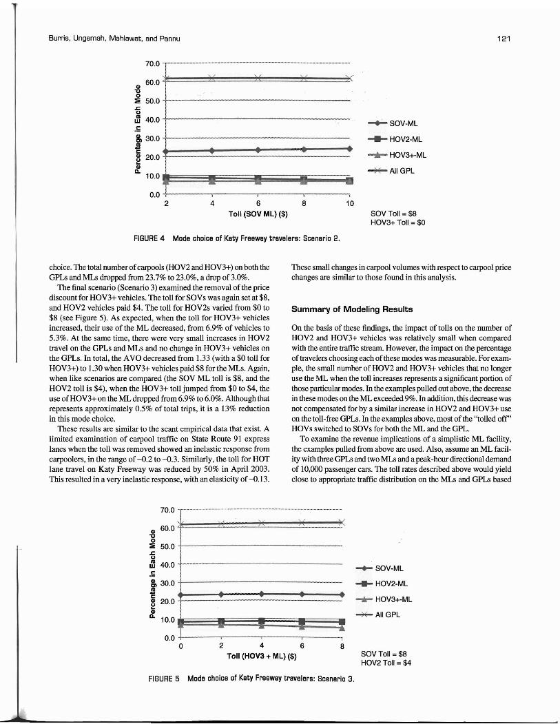
The final scenario (Scenario 3) examined the removal of the pricediscount for HOV3+ vehicles. The toll for SOYs was again set at $8,and HOV2 vehicles paid $4. The toll for HOV2s varied from $0 to$8 (see Figure 5). As expected, when the toll for HOV3+ vehiclesincreased, their use of the ML decreased, from 6.9% of vehicles to5.3%. At the same time, there were very small increases in HOV2travel on the GPLs and MLs and no change in HOV3+ vehicles onthe GPLs. In total, the AVO decreased from 1.33 (with a $0 toll forHOV3+) to 1.30 when HOV3+ vehicles paid $8 for the MLs. Again,when like scenarios are compared (the SOY ML toll is $8, and theHOV2 toll is $4), when the HOV3+ toll jumped from $0 to $4, theuse ofHOV3+on the ML dropped from 6.9% to 6.0%. Although thatrepresents approximately 0.5% of total trips, it is a 13% reductionin this mode choice.

These results are similar to the scant empirical data that exist. Alimited examination of carpool traffic on State Route 91 expresslanes when the toll was removed showed an inelastic response fromcarpoolers, in the range of -0.2 to -0.3. Similarly, the toll for HOTlane travel on Katy Freeway was reduced by 50% in April 2003.This resulted in a very inelastic response, with an elasticity of -0.13.

These small changes in carpool volumes with respect to carpool pricechanges are similar to those found in this analysis.

Summary of Modeling Results

On the basis of these findings, the impact of tolls on the number ofHOV2 and HOV3+ vehicles was relatively small when comparedwith the entire traffic stream. However, the impact on the percentageof travelers choosing each of these modes was measurable. For exam­ple, the small number of HOV2 and HOV3+ vehicles that no longeruse the ML when the toll increases represents a significant portion ofthose particular modes. In the examples pulled out above, the decreasein these modes on the ML exceeded 9%. In addition, this decrease wasnot compensated for by a similar increase in HOV2 and HOV3+ useon the toll-free GPLs. In the examples above, most of the "tolled off"HOVs switched to SOYs for both the ML and the GPL.

To examine the revenue implications of a simplistic ML facility,the examples pulled from above are used. Also, assume an ML facil­ity with three GPLs and two MLs and a peak-hour directional demandof 10,000 passenger cars. The toll rates described above would yieldclose to appropriate traffic distribution on the MLs and GPLs based

70.0 -.' -- 0 •••••••• 0 .

GI 60.0 ~==~::::=::::=~~~~~~~~"Ca::! 50.0 .,---------------­~U

~ 40.0 +-----------------.58, 30.0 +-----------------

E ~===~===~===~~==~GI 20.0':;~

~

10.0 f===~-I====-I====t:_===!_

-+- SOV-ML

.... HOV2-ML

..... HOV3+·ML

~AIIGPL

SOVToll =$8HOV2TolI=$4

8246

Toll (HOV3 + ML) ($)

0.0 +-----r-----.------r---,o

FIGURE 5 Mode choice of Katy Freeway travelers: Scenario 3.

1/

122

on this model. In Scenario 1 (with SOY toll of $8, HOV2 toll of $4,and HOV3+ toll of $0) the peak-hour revenues are $21,848 (2310 x$8 + 842 x $4 + 690 x $0). In Scenario 2 (with SOY toll of $8, HOV2toll of$8, and HOV3+toll of$0) the peak-hour revenues are $25,136(2,379 x $8 + 763 x $8 + 694 x $0), a 15.0% increase. In Scenario 3(with SOY toll of $8, HOV2 toll of $4, and HOV3+ toll of $4) thepeak-hour revenues are $24,436 (2,326 x $8 + 853 x $4 + 604 x $4),an 11.2% increase with respect to revenue generated in Scenario 1modeling.

CONCLUSIONS

This research examined the potential impacts of removing or reducingthe preferential treatment for carpools in HOV lanes. The impetusfor this is the potential for additional revenue from selling the capac­ity on the HOV lanes. However, this benefit must be weighed againstthe negative impacts on the number oftravelers who choose to carpool.

To investigate this potential impact, a survey ofHouston and Dal­las travelers was undertaken. Despite efforts to obtain a survey sam­ple that was representative of the populations of the two cities, thesurvey sample contained too few minority and low-income respon­dents. To adjust results to better reflect the population, a replicateweighting process was used. When responses were analyzed by thisweighting process, the same mean values but different standarddeviations were obtained when compared with a simple weightingprocess. This provided more accurate results when the data were exam­ined for significant differences. The survey responses were also usedto develop a mode choice model.

This mode choice model was used to predict the impact of con­verting an HOV lane to a HOT lane, where all travelers pay a toll.The model found that travelers were relatively insensitive to price.It was found that the overall percentage of HOV2 and HOV3+ vehi­cles in the traffic stream decreased by only a small amount when atoll was required for them to use the HOV lane. However, this didrepresent a significant portion of those modes (more than 9% in thespecific scenarios examined) and did result in increased HOT lanerevenue (more than 10% in the specific scenarios examined). There­fore, elimination of preferential treatment for these vehicle types hassignificant implications and becomes a difficult policy decision­not just a straightforward choice.

ACKNOWLEDGMENTS

This paper is based on research sponsored by the Texas Departmentof Transportation. The authors thank the agency for sponsorship ofthe research on which this paper is based. It was performed by theTexas Transportation Institute ofthe Texas A&M University Systemand the University of Texas at Arlington. The authors thank projectdirector Matt MacGregor and the many researchers who worked onthis project for their leadership and guidance, as well as the anonymousreviewers for their insightful comments and suggestions.

REFERENCES

1. Bureau ofTransportation Statistics. National Transportation Statistics:2005. U.S. Department of Transportation, 2005. www.bts.dot.gov/publications/national_transportation_statistics/2005/.

2. Fuhs, C., and J. Obenberger. HOV Facility Development: A Review ofNational Trends. Transportation Research Board HOV Systems Com-

Transportation Research Record 2099

mittee. Jan. 2002. www.hovworld.comlPDFslFuhs_Obenberger-final%20paper.pdf.

3. Stockton, W. R, G. Daniels (Goodin), D. Skowronek, and D. Fenno.The ABC's ofHOV: The Texas Experience. Texas Transportation Insti­tute, Texas A&M University. Sept. 1999. www.hovworld.comlPDFs/I353-Lpdf.

4. Swisher, M., W. Eisele, D. Ungemah, and G. D. Goodin. Life Cycle Graph­ical Representation ofManaged HOV Lane Evolution. Committee onHigh Occupancy Vehicle Systems, 11th International HOV Conference.Oct. 2002. www.hovworld.comlPDFs/TRB2oo3-oo2I38.pdf.

5. The Rideshare Company. Carpools: A Simple Way to Save Time, Money,and the Environment. www.commutersregister.comlctlarticles/9905/rslocal.htm.

6. Turnbull, K. F., P. A. Turner, and N. F. Lindquist. Investigation ofLandUse, Development, and Parking Policies to Support the Use of High­Occupancy Vehicles in Texas. Report No. I361-lF. Texas TransportationInstitute, College Station, 1995.

7. Crain and Associates. San Bernardino Freeway Busway EvaluationofMixed-Mode Operations. California Department of Transportation,Los Angeles, 1978.

8. Valdez, R, and C. Arce. Comparison of Travel Behavior and Attitudesof Rideshare, Solo Drivers, and the General Commuter Population. InTransportation Research Record: Journal ofthe Transportation ResearchBoard, No. 1285, TRB, National Research Council, Washington, D.C.,1990, pp. 105-108.

9. Cervero, R., and B. Griesenbeck. Factors Influencing Commuting Choicesin Suburban Labor Markets: A Case Study of Pleasanton, California.Transportation Researcher, Vol. 22A, No.3, 1998, pp. 151-161.

10. Bullard, D. L. An Assessment of Carpool Utilization of the Katy High­Occupancy Vehicle Lane and the Characteristics ofHouston's HOV LaneUsers and Nonusers. Report No. 484-14F. Texas Transportation Institute,College Station, 1991.

11. Turnbull, K. F. An Assessment ofHigh-Occupancy Vehicle Facilitiesin North America: Executive Report. Report No. 925-5F. TexasTransportation Institute, College Station, 1992.

12. Turnbull, K. F. High-Occupancy Vehicle Project Case Studies: HistoricalTrends and Project Experience. Report No. 925-4. Texas TransportationInstitute, College Station, 1992.

13. Strgar-Roscoe-Fausch, Inc. 1-394 Phase III Evaluation-Final Report.Minnesota Department of Transportation, Minneapolis, 1995.

14. Model Transportation Demand Management Program. Explore YourCommute Options: It's the SMART Thing to Do. Detailed ProgramDescription and Policy Guidelines. Washington State Department ofTransportation, Olympia. June 15, 1996. www.wsdot.wa.gov/tdrnltripreductionldownloadlCTR_Manual.pdf. Accessed May 2006.

15. Littman, T. TDM Encyclopedia: Ridesharing. Victoria Transport PolicyInstitute. Victoria, British Columbia, Canada. Dec. 14,2005. www.vtpi.orgltdrnltdm34.htm. Accessed May 2006.

16. Pollution Probe. S-M-A-R-T Movement: Save Money and the Air by Reduc­ing Trips. Pollution Probe Inc. Toronto, Ontario, Canada. Oct. 2001.www.pollutionprobe.orglReports/SMART.pdf. Accessed May 2006.

17. Poole, R., and T. Balaker. Virtual Exclusive Busways: ImprovingUrban Transit While Relieving Congestion. Policy Study 337. ReasonFoundation. Sept. 2005. www.reason.orglps337.pdf.

18. McGuckin, N., and N. Srinivasan. Journey to Work in the Context ofDailyTravel. Transportation Research Board. Census Data for TransportationPlanning Conference. May 2005. www.trb.orglconferenceslcensusdata/Resource-Journey-to-Work.pdf.

19. Chum, G. L., and M. W. Burris. Potential Mode Shift from Transit toSingle-Occupant Vehicle on a High-Occupancy-Toll Lane. In Trans­portation Research Record: Journal of the Transportation ResearchBoard, No. 2072, Transportation Research Board of the National Acad­emies, Washington, D.C., 2008, pp. 10-19.

20. Brick, J. M., D. Morganstein, and R Valliant. Analysis of ComplexSamples Using Replication. www.westat.comlwesvar/techpapers/ACS­Replication.pdf. Accessed Feb. 14,2007.

21. WesVar 4.2 Manual. User's Guide. www.westat.comlwesvar/aboutlWV4.2%20Manual.pdf. Accessed Feb. 18,2007.

The contents of this paper reflect the views of the authors, who are responsiblefor the facts and the accuracy of the data. The contents do not necessarily reflectthe official views or polices ofFHWA or the Texas Department of Transportation.

The HifIJ-Dccupancy Vehicle, Hii/l-Dccupancy Toll, and Managed Lanes Committeesponsored publication of this paper.