investigating power capping toward energy-efficient
TRANSCRIPT
Received: 2 October 2017 Revised: 15 December 2017 Accepted: 19 February 2018
DOI: 10.1002/cpe.4485
S P E C I A L I S S U E P A P E R
Investigating power capping toward energy-efficient scientificapplications
Azzam Haidar1 Heike Jagode1 Phil Vaccaro1 Asim YarKhan1
Stanimire Tomov1 Jack Dongarra1,2,3
1Innovative Computing Lab, University of
Tennessee, Knoxville, TN, USA2Oak Ridge National Laboratory, USA3University of Manchester, UK
Correspondence
Azzam Haidar, Innovative Computing Lab,
University of Tennessee, Knoxville, TN, USA.
Email: [email protected]
Funding information
National Science Foundation NSF,
Grant/Award Number: 1450429 and 1514286;
Exascale Computing Project, Grant/Award
Number: 17-SC-20-SC
Summary
The emergence of power efficiency as a primary constraint in processor and system design poses
new challenges concerning power and energy awareness for numerical libraries and scientific
applications. Power consumption also plays a major role in the design of data centers, which may
house petascale or exascale-level computing systems. At these extreme scales, understanding
and improving the energy efficiency of numerical libraries and their related applications becomes
a crucial part of the successful implementation and operation of the computing system. In this
paper, we study and investigate the practice of controlling a compute system's power usage, and
we explore how different power caps affect the performance of numerical algorithms with dif-
ferent computational intensities. Further, we determine the impact, in terms of performance and
energy usage, that these caps have on a system running scientific applications. This analysis will
enable us to characterize the types of algorithms that benefit most from these power manage-
ment schemes. Our experiments are performed using a set of representative kernels and several
popular scientific benchmarks. We quantify a number of power and performance measurements
and draw observations and conclusions that can be viewed as a roadmap to achieving energy
efficiency in the design and execution of scientific algorithms.
KEYWORDS
energy efficiency, high performance computing, Intel Xeon Phi, Knights landing, PAPI,
performance analysis, performance counters, power efficiency
1 INTRODUCTION
A fundamental challenge in the effort to reach exascale performance levels is striking the right balance between performance and power efficiency
at the appropriate software and hardware levels. In this paper, we discuss strategies for power measurement and power control to offer scientific
application developers the basic building blocks required to develop dynamic optimization strategies while working within the power constraints of
modern and future high-performance computing (HPC) systems.
Applications with high data bandwidth requirements, commonly referred to as “memory-bound” applications, have very different impli-
cations for power consumption compared to “compute-bound” problems that require heavy CPU throughput. From an energy perspective,
compute-bound workloads result in high CPU power consumption, while memory-bound workloads primarily consume power through the main
dynamic random-access memory (DRAM). In the latter case, the CPU may not need to consume power at peak levels because the main DRAM's
latency and bandwidth serve as a bottleneck. This dynamic suggests that small decrements to the CPU power limit may reduce power consumption
over time with minimal-to-no performance degradation, which ultimately results in significant energy savings.
To investigate potential power savings, a power management framework must be used for dynamic power monitoring and power capping. Ana-
lyzing how hardware components consume power at run time is key in determining which of the aforementioned categories an application fits into.
As the computing landscape evolved, hardware vendors began offering access to their energy monitoring capabilities. For example, beginning with
the introduction of the Sandy Bridge architecture, Intel incorporates the running average power limit (RAPL) model in their CPU design to provide
Concurrency Computat Pract Exper. 2018;e4485. wileyonlinelibrary.com/journal/cpe Copyright © 2018 John Wiley & Sons, Ltd. 1 of 14https://doi.org/10.1002/cpe.4485

2 of 14 HAIDAR ET AL.
estimated energy metrics. Similarly, AMD recently began incorporating power-related functionality, which is very similar to the Intel RAPL inter-
face, for modern AMD architectures. As a result, users have increasingly broad access to technology that allows them to dynamically allocate and
adjust the power consumption1 of hardware components residing within the CPUs running on their systems. These power adjustments can be based
on system-level settings, user settings, and/or the performance characteristics of the current computational workload. In general, power manage-
ment can improve the user experience under multiple constraints to increase throughput-performance and responsiveness when demanded (burst
performance) while improving things like battery life, energy usage, and noise levels when maximum performance is not required.
The primary goal of this paper is to propose a framework for understanding and managing power usage on a computer system running scientific
applications. To identify opportunities for improving the efficiency of an entire application, we study and analyze power consumption as it relates to
the computational intensity of the individual algorithms on which these kinds of applications run. Our intent is to enable energy-aware algorithmic
implementations that can execute with near-minimal performance loss. Below is a brief overview of each contribution provided in this work.
• We discuss the development of the Performance Application Programming Interface's (PAPI's) “powercap” component, which uses the Linux
powercap interface to expose the RAPL settings to user-space. This new powercap component has an active interface to allow writing values
in addition to reading them. This is a significant change from the RAPL-based components provided in previous versions of PAPI, which had
an entirely passive read-only interface. Having this power capping functionality available through the de facto standard PAPI interface pro-
vides portability and is beneficial to many scientific application developers, regardless of whether they use PAPI directly or use third-party
performance toolkits.
• We present a study of the correlation between power usage and performance for three different types of numerical kernels that are representative
of a wide range of real scientific applications. This study provides us with a clear understanding of the factors that contribute to energy savings
and performance. We are using the proposed power control mechanism because we are interested not only in reducing power usage, but also,
perhaps more importantly, we are interested in exploring energy savings with minimal impact on an application's execution time.
• We extend our study of power usage and performance from numerical kernels to mini apps and scientific applications in order to validate our
observations of power capping's effectiveness.
• This paper goes beyond performance and power measurements by also providing a detailed analysis of the capping techniques and present-
ing a collection of lessons that will enable researchers to understand and develop their own computational kernels in a simple and efficient
energy-aware fashion. We introduce a framework for power information and power capping and describe the path to an energy-aware model
that will enable developers to predict the likely performance/energy efficiency of their kernels using a structured approach.
• To our knowledge, this is the first paper that evaluates the power efficiency and power capping as it relates to the algorithmic intensity on
Intel's Knights Landing (KNL) architecture, and we aim to provide information that will enable researchers to understand and predict what
to expect from managing power on this architecture and from using high-bandwidth multi-channel DRAM (MCDRAM) memory over standard
fourth-generation double data rate (DDR4) synchronous DRAM memory.
The rest of the paper is organized as follows. Section 2 describes the power management mechanisms that we propose and use. Next, in Section 3,
we present our experimental approach, followed by experimental results and discussion on kernels and selected mini-apps (in Section 4). Section 5
is on related work. Finally, Section 6 is on conclusions, summarizing the contributions of this paper.
2 POWER MANAGEMENT
Various techniques exist for monitoring and limiting power that take advantage of recent hardware advances. Each technique is known to have
unique implications regarding accuracy, performance overhead, and ease of use, and there are two basic aspects that make up a power monitoring
framework. First, there is an underlying model that specifies the mechanics for how power is measured and how power limits are applied through
the hardware counters. Second, a software package is employed that interfaces with a given model to provide users with a means for interacting
with the various power controls provided. In general, the monitoring capabilities (reporting power measurements) are standard across the range of
options. However, there is a distinction when examining how the various frameworks apply power limits on systems. For this work, we chose RAPL,
which estimates energy metrics with decent accuracy and has enjoyed the most popularity in the computing community.
2.1 RAPL, powercap, and power-limiting mechanisms
Dynamic voltage and frequency scaling (DVFS) is a common technique used to exercise control over a hardware component's power consumption.
For instance, lowering the clock frequency of a processor results in a reduced number of instructions that the processor can issue in a given amount
of time, but since the frequency at which the circuit is clocked determines the voltage required to run it, a decrease in the voltage supply allows a
corresponding decrease in the clock frequency. This voltage decrease can yield a significant reduction in power consumption but not necessarily
energy savings, owing to rising static power consumption and reduced dynamic power range.2

HAIDAR ET AL. 3 of 14
RAPL, the primary interface used to interact with power controls on Intel hardware, provides power meter capabilities through a set of counters
that estimate energy and power consumption rates based on an internal software model. RAPL provides power-limiting capabilities on processor
packages and memory by enabling a user to dynamically specify average power consumption over a user-specified time period. There are two power
constraints that can be set: (1) a short-term power constraint that corresponds to burst responsiveness and (2) a long-term power constraint that
corresponds to throughput performance. Under the hood, the RAPL capping capability uses DVFS scaling. At low power levels, however, RAPL uses
clock cycling modulation or duty cycling modulation to force the components inside the physical package into an idle state. This modulation is done
because DVFS can lead to degradations in performance and accuracy at power levels significantly below the thermal design point (TDP) of a given
processor. It is also worth noting that using the RAPL interfaces has security and performance implications and would require applications to have
elevated privileges in most cases.
The most recent addition to the array of power monitoring options is the powercap Linux kernel interface. The purpose of this interface is to
expose the RAPL settings to the user. Powercap exposes an intuitive sysfs tree representing all of the power “zones” of a processor. These zones
represent different parts of a processor that support power monitoring capabilities. The top level zone is the CPU package that contains “subzones,”,
which can be associated with core, graphics, and DRAM power attributes. Depending on the system, only a subset of the subzones may be avail-
able. For example, Sandy Bridge processors have two packages, each having core, graphics, and DRAM subzones, which, in addition, allows for the
calculation of uncore (last level caches, memory controller) power by simply subtracting core and graphics from package. On the other hand, KNL
processors have a single package containing only core and DRAM subzones. Power measurements can be collected, and power limits enforced, at
the zone or the subzone level. Applying a power limit at the package level will also affect all of the subzones in that package.
2.2 PAPI: The Performance API
The PAPI performance monitoring library provides a coherent methodology and standardization layer to performance counter information for a
variety of hardware and software components, including CPUs,3 graphics processing units (GPUs),4 memory, networks,5,6 I/O systems,3 power
systems,7,8 and virtual cloud environments.9PAPI can be used independently as a performance monitoring library and tool for application analysis;
however, PAPI finds its greatest utility as a middleware component for a number of third-party profiling, tracing, and sampling toolkits (eg, CrayPat,10
HPCToolkit,11 Scalasca,12 Score-P,13 TAU,14 Vampir,15 PerfExpert16), making it the de facto standard for performance counter analysis. As a middle-
ware, PAPI handles the details for each hardware component to provide a consistent application programming interface (API) for the higher-level
toolkits. PAPI also provides operating system-independent access to performance counters within CPUs, GPUs, and the system as a whole.
2.3 Adding a powercap component to PAPI
Energy consumption has been identified as a major concern for extreme-scale platforms,17 and PAPI offers a number of components for different
architectures that enable transparent monitoring of power usage and energy consumption through different interfaces. In the past, the PAPI power
components only supported reading power information from the hardware. However, PAPI now includes a newly developed component that extends
its power measurements by wrapping around the Linux powercap kernel interface, which exposes RAPL functionality through thesysfs directory
tree. This new powercap component provides a simple interface that enables users to monitor and limit power on supported Intel processors. The
component accomplishes this by dynamically discovering the available power attributes of a given system and exposing (to the user) the ability to
read and set these attributes. This component provides an advantage over using other PAPI components for power (eg, RAPL) because it does not
require root access in order to read power information. This increases the ease of use for those who wish to obtain control over power attributes
for high-performance applications.
The powercap component exposes power attributes that can be read to retrieve their values and a smaller set of attributes that can be
written to set system variables. All power attributes are mapped to events in PAPI, which matches its well-understood format. A user can employ our
component to collect statistics from all or some of these attributes by specifying the appropriate event names. A user could also write a small test
application that uses the component to poll the appropriate events for energy statistics at regular intervals. This information could then be logged
for later analysis. Also, a user can create a test program that applies power limits at any of the power “zones” discussed in the previous section by
specifying the appropriate event names in the component. For example, one could apply separate power limits for DRAM than for core events on a
CPU package. Alternatively, a power limit could be applied one level up in the hierarchy at the CPU package level. With this added flexibility, which is
the result of our development on this component, the powercap component can aid a user in finding opportunities for energy efficiency within each
application. For instance, the component can help a user choose between several different algorithmic implementations of an operation, enabling
the user to find the most energy-efficient algorithms for a given application.8,17
Although power optimization opportunities may not be present in every algorithm, PAPI with its powercap component can provide the infor-
mation that a user or developer needs to make that determination (eg, read power consumption, FLOPS computed, memory accesses required by
tasks), and it provides the API that allows an application to control power-aware hardware.

4 of 14 HAIDAR ET AL.
Even though the research presented in this work focuses on Intel CPUs, it is generally applicable to other architectures. In fact, although the Linux
powercap sysfs interface has only been implemented for Intel processors, it could be extended to other architectures in the future. Additionally,
PAPI provides other components that enable users to access power metrics on other architectures. For example, on AMD Family 15h machines,
power can be accessed with the PAPI lmsensors component; for IBM BlueGene/Q, PAPI provides the emon component; and for NVIDIA GPUs,
PAPI provides the nvml component. These components are currently accessed as read only, but PAPI can enable power capping should the vendor
provide such capability.
3 EXPERIMENTAL APPROACH
The goal of this work is to gain insight into the effects that dynamic power adjustments have on HPC workloads. Our intent is to understand and pro-
vide lessons on how we can enable an application to execute with near-minimal performance loss with improved energy efficiency. Applications with
high data bandwidth requirements, commonly referred to as memory-bound applications, have very different implications for power consumption
compared to compute-bound problems that require heavy CPU throughput. From an energy perspective, compute-bound workloads result in high
CPU power consumption, while memory-bound workloads primarily consume power based on the throughput of the main dynamic random-access
memory (DRAM). In the latter case, the CPU may not need to consume power at peak levels because the main DRAM's latency and bandwidth serve
as a bottleneck. This dynamic suggests that small decrements to the CPU power cap may reduce power consumption over time with minimal-to-no
performance degradation, which ultimately results in significant energy savings. we would like to propose a framework for understanding and man-
aging the power use of scientific applications in order to provide energy awareness. To identify opportunities for improving the efficiency of an
application, a study on analyzing power consumption is key to determining into which of the aforementioned categories it fits. Thus, since the power
consumption is correlated to the computational intensity of the individual kernels on which these kinds of applications run, we carefully perform our
study through a set of representative examples from linear algebra that exhibit specific computational characteristics and from a set of well-known
scientific benchmarks that are representatives of many real life applications.
Many hardware vendors offer access to their energy monitoring capabilities in terms of measurement or management. As a result, users have
increasingly broad access to technology that allows them to allocate and adjust the power of hardware components residing within the CPUs run-
ning on their systems. To gain access to a power management interface, we use the PAPI powercap component mentioned in the previous section.
This interface enables a user to easily instrument an application with power monitoring and power capping functionality. To execute tests, a probing
framework was designed using the PAPI powercap API, which takes in an arbitrary program, starts collecting power measurements, applies a power
limit, executes the test program, resets the power limit to the default value, and then stops collecting power measurements. This data is then used
as the basis for the analysis.
3.1 Testing environment
Tests were conducted on an Intel Xeon Phi KNL 7250 processor with 68 cores and two levels of memory. The larger primary memory (DDR4) has a
capacity of up to 384 GB, and the second high-speed memory (MCDRAM) has a capacity of up to 16 GB. The primary distinction between the two
is that MCDRAM resides on the processor die itself and its data transfer rate outperforms DDR4 by a factor of four. This is important because KNL
processors have the ability to be configured in one of three memory modes: cache, flat, or hybrid. Cache mode treats the MCDRAM as a traditional
cache (last-level cache, to be precise), which is used transparently by the cores on the non-uniform memory access (NUMA) node. In flat mode,
NUMA node 0 houses the DDR4 memory and all of the CPU cores, and NUMA node 1 contains the high-speed MCDRAM, where data is explicitly
allocated by the user. In hybrid mode, NUMA node 0 houses the DDR4 along with half (8 GB) of the MCDRAM as cache, and NUMA node 1 holds
the remaining half (8 GB) of the MCDRAM to be allocated and managed explicitly.
Note that, for the cache mode, the data must be allocated to the DDR4 initially; however, if the data is less than 16 GB it will be retained in the
cache (in the MCDRAM) after it has been used, and it will behave as if the operation was running in flat mode with the data allocated to the MCDRAM
thereafter. For hybrid mode, there are two options for allocating the data: in the MCDRAM or in the DDR4. When data is allocated in the MCDRAM,
the hybrid mode operates in a similar fashion as flat mode. When data is allocated in the DDR4, and its size is less then 8 GB, it will behave roughly
as if it was allocated in the MCDRAM using flat mode because it will be cached; however, if the data exceeds 8 GB, there will be about 8 GB of data
held in cache (in the MCDRAM), which makes it very difficult to study the behavior of the DDR4. For flat mode, the data is either in the MCDRAM
or in the DDR4 and is allocated and managed explicitly in one of those locations.
All of the experiments in this work were carried out using memory in flat mode because the performance behavior of flat mode sufficiently repre-
sents the performance seen in the rest of the memory modes. If the data is less that 8 GB and is allocated to the MCDRAM, then flat mode behaves
like cache mode or hybrid mode after the first touch. If a large amount of data is allocated in the DDR4, then the flat mode memory behavior is con-
strained by the DDR4's performance characteristics and will be similar in all memory modes. To explore the energy implications of different NUMA

HAIDAR ET AL. 5 of 14
TABLE 1 Power metrics available on Intel's KNL
Power Attributes and Descriptions
PACKAGE_ENERGY(R):
Energy consumption of the entire CPU (ie, cores subsystem, MCDRAM, memory controller,
2-D mesh interconnect), not including the DDR4 memory.
PACKAGE_SHORT_TERM_POWER_LIMIT(R/W):
Upper average power bound within the package short-term time window.
PACKAGE_LONG_TERM_POWER_LIMIT(R/W):
Upper average power bound within the package long-term time window.
PACKAGE_SHORT_TERM_TIME_WINDOW(R/W):
Time window associated with package short-term power limit.
PACKAGE_LONG_TERM_TIME_WINDOW(R/W):
Time window associated with package long-term power limit.
DRAM_ENERGY(R):
Energy consumption of the off-package memory (DDR4).
DRAM_LONG_TERM_POWER_LIMIT(R/W):
Upper average power bound within the DRAM long-term time window.
DRAM_LONG_TERM_TIME_WINDOW(R/W):
Time window associated with DRAM long-term power limit.
nodes, the numactl command line tool is used to specify a NUMA node for memory allocation before the tests are executed. This tool forces the
memory to be allocated on the DDR4 or MCDRAM residing on the specified NUMA node.
3.2 Power attributes
Table 1 provides a list of events that a user can choose from to obtain energy/power readings for an application running on the Intel Xeon Phi KNL
processor. The two power domains supported on KNL are power for the entire package (PACKAGE_ENERGY) and power for the memory subsystem
(DRAM_ENERGY). As mentioned in Section 3.1, the MCDRAM is an on-package memory that resides on the processor die. For that reason, energy
consumption for the MCDRAM is included in the PACKAGE_ENERGY domain, while DDR4 is accounted for in DRAM_ENERGY domain. To have a
consistent set of tests, power measurements and power limits were collected and applied at thePACKAGE level in the hierarchy. When a power limit
is applied at the PACKAGE level, there is an implicit power limit adjustment applied at the DRAM since it is a “child” of PACKAGE in the powercap
semantics. All other writable power attributes are left to their default values for the duration of testing. However, power measurements are collected
for analysis at both thePACKAGE andDRAM levels. Note that, according to the Intel MSR documentation,18(p37) the PACKAGE domain has two power
limit/widows (a short and a long term), while the DRAM domain has only the long term one. In our experiments, as mentioned above, we left the
power limit (short and long) as well as the power windows (short and long) to their default values. We also note that the sampling rate used in our
experiment is 100 ms. A deviation of less than 3% in the power measurement was observed between different runs of the same experiment.
4 DISCUSSION
Representative workloads with specific computational characteristics were chosen from linear algebra routines and well-known scientific bench-
marks. The linear algebra routines chosen were dgemm, dgemv, and daxpy. Other workloads that represent larger scientific applications are the
Jacobi algorithm, a Lattice Boltzmann benchmark, the XSBench kernel from a Monte Carlo neutronics application, and the High Performance Con-
jugate Gradient (HPCG) benchmark. Each of these workloads is instrumented with power measurement and power limiting capabilities using the
probing framework outlined in Section 3.
4.1 Representative kernel study
To study and analyze the effect of real applications on power consumption and energy requirements, we chose kernels that can be found in HPC
applications and that can be distinctly classified by their computational intensity. The idea is that, through this analysis, we will be able to draw
lessons that help developers understand and predict the possible trade offs in performance and energy savings of their respective applications. We
decided to perform an extensive study that covers several linear algebra kernels and basic linear algebra subroutines (BLAS) in particular because
they are at the core of many scientific applications (eg, climate modeling, computational fluid dynamics simulations, materials science simulations).

6 of 14 HAIDAR ET AL.
BLAS routines are available through highly optimized libraries on most platforms and are used in many large-scale scientific application codes.
These routines consist of operations on matrices and vectors (eg, vector addition, scalar multiplication, dot products, linear combinations, and matrix
multiplication) and are categorized into three different levels, determined by operation type. Level 1 addresses scalar and vector operations, level 2
addresses matrix-vector operations, and level 3 addresses matrix-matrix operations.
First, we study the daxpy level-1 BLAS routine, which multiplies a scalar 𝛼 with a vector x and adds the results to another vector y such that y =𝛼x+ y. For the 2n floating point operations (FLOPs) (multiply and add), daxpy reads 2n doubles and writes n doubles back. On modern architectures,
such an operation is bandwidth/communication limited by the memory. An optimized implementation of daxpy might reach the peak bandwidth for
large vector sizes, but, in terms of computational performance, it will only reach about 5%-10% of a compute system's theoretical peak. Usually,
the linear algebra community prefers to show attainable bandwidth in gigabytes per second (GB/s) rather than floating point operations per second
(FLOPS/s).
Second, we examine the dgemv level-2 BLAS routine, which is a matrix-vector operation that computes y = 𝛼Ax + 𝛽y; where A is a matrix; x, y are
vectors; and𝛼, 𝛽 are scalar values. This routine performs 2n2 FLOPs on (n2+3n) ∗ 8 bytes for read and write operations, resulting in a data movement
of approximately (8n2 + 24n)∕2n2 = 4 + 12∕n bytes per FLOP. When executing a dgemv on matrices of size n, each FLOP uses 4 + 12∕n bytes of
data. With an increasing matrix size, the number of bytes required per FLOP stalls at 4 bytes, which also results in bandwidth-bound operations. The
difference here, compared to daxpy, is that when the processor slows too much, the performance of dgemv might be affected more than the daxpy.
The third routine we study is the dgemm level-3 BLAS routine, which performs a matrix-matrix multiplication computing C = 𝛼AB + 𝛽C; where
A,B,C are all matrices; and 𝛼, 𝛽 are scalar values. This routine performs 2n3 FLOPs (multiply and add) for 4n2 data movements, reading the A,B,C
matrices and writing the results back to C. This means that dgemm has a bytes-to-FLOP ratio of (4n2 ∗ 8)∕2n3 = 16∕n. When executing a dgemm
on matrices of size n, each FLOP uses 16∕n bytes of data. This routine is characterized as compute-intensive and is bound by the computational
capacity of the hardware and not by the memory bandwidth. As the size of the matrix increases, the number of bytes required per FLOP decreases
until the peak performance of the processor is reached. The dgemm has a high data reuse, which allows it to scale with the problem size until the
performance is near the machine's peak.
All plots in this section adhere to the following conventions for displaying data. To quantify the effect of power capping on performance and to
study the behavior of each routine, we fixed the problem size (eg, matrix or vector size) and ran each experiment for 10 iterations. For each iteration,
we dropped the power in 10 or 20 Watts steps, starting at 220 Watts and bottoming out at 120 Watts. The plotted data includes the applied power
cap (black curve), the processor's clock frequency (orange curve), the package power that includes the MCDRAM power (green curve), and the
DRAM power (cyan curve). Thus, each “step" shown in the graph reflects a new power limit that was applied before the execution of the operation.
Note that the plotted power limit (black curve) is collected using the instrumentation tool after it is explicitly set by the powercap component. This
serves as a sanity check to verify that a power limit applied through the powercap component is actually accepted and enforced by the Linux kernel.
4.2 Study of the dgemm routine
Figure 1 shows the power data collected from a dgemm operation that was instrumented with the PAPI powercap tool. Figure 1A shows executions
with data allocated to NUMA node 0 (DDR4), and Figure 1B shows executions with data allocated to NUMA node 1 (MCDRAM). Since the dgemm
Time (sec)0 10 20 30 40 50 60 70 80 90 100 110
Ave
rag
e p
ow
er (
Wat
ts)
020406080
100120140160180200220240260280300320
1991
8.22
1383
1901
8.36
1341
1785
8.58
1314
1615
8.57
1325
1340
8.02
1419
1154
7.36
1562
971
6.66
1715
785
5.81
1982
575
4.64
2489
Performancein Gflop/s
Gflops/Watts
Joules
Accelerator Power Usage (PACKAGE)Memory Power Usage (DDR4)Max power limit set
MH
z
0 200 400 600 800 100012001400160018002000
Frequency
(A)Time (sec)
0 10 20 30 40 50 60 70 80 90 100 110
Ave
rag
e p
ow
er (
Wat
ts)
020406080
100120140160180200220240260280300320
1997
8.82
1303
1904
8.92
1279
1741
8.95
1267
1589
9.04
1253
1328
8.47
1345
1137
7.73
1480
956
6.95
1661
773
6.03
1904
560
4.72
2443
Performancein Gflop/s
Gflops/Watts
Joules
Accelerator Power Usage (PACKAGE)Memory Power Usage (DDR4)Max power limit set
MH
z
0 200 400 600 800 100012001400160018002000
Frequency
(B)
FIGURE 1 Average power measurements (Watts on y axis) of the dgemm level-3 BLAS routine when the KNL is in FLAT mode. The dgemmroutine is run repeatedly for a fixed matrix size of 18 000 × 18 000. For each iteration, we dropped the power in 10-Watt or 20-Watt decrements,starting at 220 Watts and bottoming out at 120 Watts. The processor clock frequency, as measured at each power level, is shown on the right axis.A, FLAT mode: dgemm: data allocated to DDR4; B, FLAT mode: dgemm: data allocated to MCDRAM

HAIDAR ET AL. 7 of 14
routine is known to be compute intensive and underclocking and undervolting the processor is part of our energy-saving strategy, we did not expect
to obtain any energy savings without a corresponding drop in performance. In both graphs, we can see that the performance of the dgemm routine
drops as the power limit is set lower. Also, as Figure 1 illustrates, the performance of a compute-intensive routine is independent of the data-access
bandwidth; in fact, we observe that both data allocations provide roughly the same performance. This is because the FLOPs-to-bytes ratio for
compute-intensive routines is high, which allows such an implementation to efficiently reuse the low-level caches, thereby hiding the bandwidth
costs associated with transferring the data to/from memory.
Moreover, Figure 1 provides valuable information for three observations:
1. Results like these are a clear indication that this type of routine is skewed toward high algorithmic intensity rather than memory utilization.
Understanding that a given application has high algorithmic intensity could prompt exploration into possible optimizations that trade execution
time for power.
2. This figure provides confirmation that the powercap component, which uses RAPL, achieves its power limiting though DVFS scaling. This
evidence can be seen in the frequency value, which, as it drops, corresponds to a decrease in power.
3. Finally, we can confirm that the power consumption of the MCDRAM on KNL processors is not reported in the DRAM power values (cyan curve).
This can be confirmed by comparing the cyan curves representing DRAM power consumption in both Figure 1A and Figure 1B. When data is
allocated to the DDR4, the power consumed by the DRAM is high, around 22 Watts (Figure 1A). However, when the data is allocated to the
MCDRAM, the power consumed by the DRAM is only 6 Watts (Figure 1B).
Additionally, in Figure 1, we show the GFLOP/s per Watt efficiency rate at each power cap value (yellow numbers). For someone more interested in
energy efficiency than performance, we can see that even though dgemm is a compute-intensive kernel, sometimes, a lower power cap can provide
similar or even a slightly higher GFLOP/s per Watt rate. For example, setting the power limit at 220 Watts, 200 Watts, or 180 Watts will provide a sim-
ilar GFLOP/s per Watt ratio. Note, however, that a very low power cap will dramatically affect the performance and efficiency of compute-intensive
routines like dgemm.
4.3 Study of the dgemv routine
Bandwidth-limited applications are characterized by memory-bound algorithms that perform relatively few FLOPs per memory access. For these
types of routines, which have low arithmetic intensity, the floating-point capabilities of the processor are generally not important, rather, the mem-
ory latency and bandwidth limit the application's performance. We performed a set of experiments similar to our dgemm investigation to analyze
the power consumption and the performance behavior of the dgemv level-2 BLAS kernel. It is useful to show the bandwidth achieved with different
power limits since bandwidth is the key factor that determines the performance. When the peak hardware bandwidth is achieved, there is no addi-
tional performance to gain because the hardware itself will be at its theoretical peak. Since dgemv reads n2 elements to perform 2n2 operations, the
peak performance, a highly optimized implementation of dgemv in double precision (8 bytes), can reach is bandwidth∕4, where bandwidth is approx.
90 GB/s for DDR4 and ∼425 GB/s for MCDRAM.
Unlike dgemm, the majority of the execution time in dgemv is spent on memory operations, as depicted in Figures 2A and 2B. In Figure 2B, we
observe that capping the power from 220 Watts down to 180 Watts does not affect the performance of dgemv. This results in a power saving of
Time (sec)0 11 22 33 44 55 66 77 88 99 110 121 132 143 154
Ave
rag
e p
ow
er (
Wat
ts)
020406080
100120140160180200220240260280300320
2185
0.12
2588
2185
0.12
2623
2185
0.12
2639
2185
0.12
2664
2185
0.12
2661
2184
0.13
2558
2182
0.13
2432
2082
0.14
2305
1978
0.14
2240
Performancein Gflop/sAchievedBandwidth GB/sGflops/Watts
Joules
Accelerator Power Usage (PACKAGE)Memory Power Usage (DDR4)Max power limit set
MH
z
0 200 400 600 800 100012001400160018002000
Frequency
(A)Time (sec)
0 4 8 12 16 20 24 28 32 36 40 44 48 52 56 60 64
Ave
rag
e p
ow
er (
Wat
ts)
020406080
100120140160180200220240260280300320
8433
50.
3981
5
8333
10.
3980
5
8232
80.
4271
7
7931
70.
4568
6
6526
10.
4274
5
5622
50.
3882
2
4718
80.
3490
9
3815
00.
2910
77
2811
10.
2413
61
Performancein Gflop/sAchievedBandwidth GB/sGflops/Watts
Joules
Accelerator Power Usage (PACKAGE)Memory Power Usage (DDR4)Max power limit set
MH
z
0 200 400 600 800 100012001400160018002000
Frequency
(B)
FIGURE 2 Average power measurements (Watts on y axis) of the dgemv level-2 BLAS routine when the KNL is in FLAT mode. The dgemv routine isrun repeatedly for a fixed matrix size of 18 000 × 18 000. For each iteration, we dropped the power cap in 10-Watt or 20-Watt decrements, startingat 220 Watts and bottoming out at 120 Watts. A, FLAT mode: dgemv: data allocated to DDR4; B, FLAT mode: dgemv: data allocated to MCDRAM

8 of 14 HAIDAR ET AL.
40 Watts while maintaining the same performance (GFlop/s) and the same time to solution. Similarly, this trend can be noted in the energy efficiency
values (numbers in yellow or black), where a power limit between 220 Watts and 180 Watts renders in approx. 15% of energy saving with a negligible
performance penalty (of less than 5%). Moving the cap below 180 Watts, however, significantly degrades the performance.
Figure 2A shows the dgemv results with the data allocated to the DDR4 memory. Since dgemv is memory bound, we expect a different behavior
when allocating data to the DDR4 versus MCDRAM given that the two memory types have very different bandwidths. Compared to Figure 2B (data
in MCDRAM), it is clear in Figure 2A that even when the power limit is set above 160 Watts, the DDR4 bandwidth slows the CPU performance to
the point that the CPU only needs about 160 Watts to continue successful and meaningful computation.
For DDR4, we observed an average power consumption of around 35 Watts on our KNL machine. The cyan curve in Figure 2A shows that the
DDR4 was being utilized at maximum power during the entire execution. This results in lower CPU utilization and power consumption since the
DDR4 performance is the primary bottleneck. The data shown in the Figure clarifies a historical misconception that capping power consumption
always provides a benefit for memory-bound kernels. If the CPU's power consumption is already low, then power capping will not have any effect
unless it is set lower than the CPU's internal throttling. For our dgemv DDR4 allocation case, setting the power level above 180 Watts does not
make any difference and will not render any change in energy usage. On the other hand, once we reach the point where forcing a power limit has an
effect (lower than 180 Watts), we observe characteristics similar to our MCDRAM allocation case. For example, neither the performance nor the
bandwidth are affected as we move the power cap from 180 Watts down to 140 Watts; however we do start to see appreciable energy savings here,
around 10% savings at 140 Watts. Furthermore, capping the power at 120 Watts results in 17% energy savings with some performance degradation
(∼8%).
When comparing the two storage options overall, the performance is very different. For MCDRAM data allocations, the performance is about 4×higher compared to DDR4 data allocations. This is expected since MCDRAM provides a bandwidth of about 425 GB/s, whereas DDR4 provides only
about 90 GB/s. In terms of total energy (DRAM + PACKAGE energy), the 4× increase in performance results in a more than 3× benefit in energy
savings when using MCDRAM over DDR4.
Based on our experiment with a memory-bound routine, we learned that it is possible to obtain significant energy savings without any real loss
in performance. Overall, capping the package power at around 40 Watts below the (observed) power draw of the default setting provides about
15%-17% energy savings without any significant reduction in the time to solution.
Note that capping DRAM power (below its default power consumption) for dgemv (memory bound kernels) will affect the time-to-solution of the
memory bound kernel, however, most likely not in a beneficial way that allows for energy savings. For that, we do not perform DRAM capping in this
paper.
4.4 Study of the daxpy routine
To complete our examination of all three levels of BLAS routines, a similar set of experiments was performed for the daxpy level-1 BLAS routine.
We observed similar outcomes with daxpy as we did with the dgemv kernel. The performance of the MCDRAM option is on average approx. 4×higher than the DDR4 option, for the same reason: MCDRAM provides about 4× higher memory bandwidth. As shown in both graphs of Figure 3,
the power limits used for these tests started at 220 Watts and were stepped down to 120 Watts in 20- or 10-Watt decrements.
Time (sec)0 8 16 24 32 40 48 56 64 72 80 88 96 104 112 120
Ave
rag
e p
ow
er (
Wat
ts)
020406080
100120140160180200220240260280300320
787
0.04
2080
787
0.04
2076
787
0.04
2098
787
0.04
2094
785
0.04
1993
784
0.04
1871
784
0.04
1802
782
0.05
1700
666
0.04
1951
Performancein Gflop/sAchievedBandwidth GB/sGflops/Watts
Joules
Accelerator Power Usage (PACKAGE)Memory Power Usage (DDR4)Max power limit set
MH
z
0 200 400 600 800 100012001400160018002000
Frequency
(A)Time (sec)
0 3 6 9 12 15 18 21 24 27 30 33 36 39 42 45 48
Ave
rag
e p
ow
er (
Wat
ts)
020406080
100120140160180200220240260280300320
3542
00.
1551
235
416
0.16
465
3441
00.
1742
529
344
0.16
443
2226
30.
1454
5
1922
60.
1361
4
1518
50.
1168
6
1214
40.
0984
4
910
50.
0710
65
Performancein Gflop/sAchievedBandwidth GB/sGflops/Watts
Joules
Accelerator Power Usage (PACKAGE)Memory Power Usage (DDR4)Max power limit set
MH
z
0 200 400 600 800 100012001400160018002000
Frequency
(B)
FIGURE 3 Average power measurements (Watts on y axis) of the daxpy level-1 BLAS routine when the KNL is in FLAT mode. The daxpy routine isrun repeatedly for a fixed vector of length 106 per step. At each iteration, we dropped the power cap in 10-Watt or 20-Watt decrements, startingat 220 Watts and bottoming out at 120 Watts. A, FLAT mode: daxpy: data allocated to DDR4; B, FLAT mode: daxpy: data allocated to MCDRAM

HAIDAR ET AL. 9 of 14
The primary takeaway from the data shown in Figure 3B is that, for MCDRAM storage, the execution times for power limits of 220-180 Watts,
are all nearly identical. Below 180 Watts, the performance begins to degrade; again, this is similar to the dgemv results. These findings show that
when running a dgemv or daxpy memory-bound routine with data allocated to the MCDRAM, performance is unchanged when power is capped
anywhere in the 220-180–Watt range. When the data is allocated to DDR4; however, the power can be capped at 130 Watts without significantly
affecting performance, as can be observed from Figure 3A.
Ultimately, this lower power cap can provide significant energy savings if many instances of these memory-bound workloads are needed (eg,
iterative simulation schema or computational fluid dynamics simulations where a Jacobi or Lattice Boltzmann iteration must be used). This infor-
mation validates the notion that energy savings for memory-bound computational workloads can be attained relatively easily by applying modest
power caps.
4.5 Benchmarks and mini-applications
To confirm the findings that we observed during our experiments with the three levels of BLAS kernels, all of which have different computational
intensities, we ran tests (with power caps) on a number of larger benchmark applications and other mini-apps that are more representative of
real-world scientific applications. These benchmarks and mini-apps include the Jacobi application, the Lattice Boltzmann (LBM) benchmark, the
High Performance Conjugate Gradient (HPCG) benchmark, the XSBench mini-app, and the Stream benchmark.
To evaluate the power efficiency and gain for every application described here, we launch the application under a power cap limit and mea-
sure its performance (the mean elapsed time required for completion) and its power consumption (CPU package). For each application, two sets of
experiments are performed: (1) with the data allocated to the DDR4 and (2) with the data allocated to the MCDRAM. Every graph consists of 5-6
experiments where we solve the same problem with a different power cap. We used the same problem size for each experiment so that the x axis
(time) reflects the real computation time, which allows us to compute the percentage of power gain and/or time delay that occurs. Our findings for
each application are presented in the following subsections.
4.5.1 Jacobi application
The Jacobi application used in our testing solves a finite difference discretization of the Helmholtz equation using the Jacobi iterative method. The
Jacobi method implements a 2-D, five-point stencil that requires multiple memory accesses per update. This means that the application has a high
memory bandwidth and has a low computational intensity. This application is comparable to daxpy, and we expect that the lessons learned from our
experiments with daxpy will enable us to find power savings for the Jacobi application.
Figure 4 presents the power consumption of the CPU package when running the Jacobi algorithm on a 12 800 × 12 800 grid with data allocated
to the DDR4 (left) and the MCDRAM (right). The x axis represents the time required to finish the computation, which reflects the achievable per-
formance for each power cap. The experiments show that, when data is allocated to the MCDRAM (Figure 4B), the power cap can range from 205
Watts down to 170 Watts without any loss of performance. That means, at 170 Watts, the application's time to solution does not change, but the
application consumes around 14% less energy. Dropping the cap to 155 Watts renders only a slight increase in the time to solution but saves even
Time (sec)0 2 4 6 8 10 12 14 16 18 20 22 24 26 28 30 32
Ave
rag
e p
ow
er (
Wat
ts)
020406080
100120140160180200220240260280300
2770 joules2878 joules2689 joules2438 joules2137 joules
2731 joules
DDR_215WattsDDR_200WattsDDR_180WattsDDR_160WattsDDR_140WattsDDR_120Watts
(A)
Time (sec)0 1 2 3 4 5 6 7 8 9 10 11 12 13 14 15 16 17 18 19 20 21 22
Ave
rag
e p
ow
er (
Wat
ts)
020406080
100120140160180200220240260280300
826 joules842 joules
724 joules
803 joules
1066 joules
1865 joules
MCDRAM_215WattsMCDRAM_200WattsMCDRAM_180WattsMCDRAM_160WattsMCDRAM_140WattsMCDRAM_120Watts
(B)
FIGURE 4 Average power measurements (Watts on y axis) of Jacobi algorithm on a 12 800 × 12 800 grid for different power caps. DDR4 on theleft. MCDRAM on the right. A, FLAT mode: data allocated to DDR4; B, FLAT mode: data allocated to MCDRAM
10 of 14 HAIDAR ET AL.
Time (sec)0 4 8 12 16 20 24 28 32 36 40 44 48 52 56 60 64 68
Ave
rag
e p
ow
er (
Wat
ts)
020406080
100120140160180200220240260280300
9064 joules9196 joules9194 joules9178 joules9005 joules8084 joules
8467 joules
DDR_270wattsDDR_215wattsDDR_200wattsDDR_180wattsDDR_160wattsDDR_140wattsDDR_120watts
(A)
Time (sec)0 3 6 9 12 15 18 21 24 27 30 33 36 39 42 45 48 51 54
Ave
rag
e p
ow
er (
Wat
ts)
020406080
100120140160180200220240260280300
3050 joules
2981 joules
2872 joules
3043 joules3383 joules
4033 joules5734 joules
MCDRAM_270wattsMCDRAM_215wattsMCDRAM_200wattsMCDRAM_180wattsMCDRAM_160wattsMCDRAM_140wattsMCDRAM_120watts
(B)
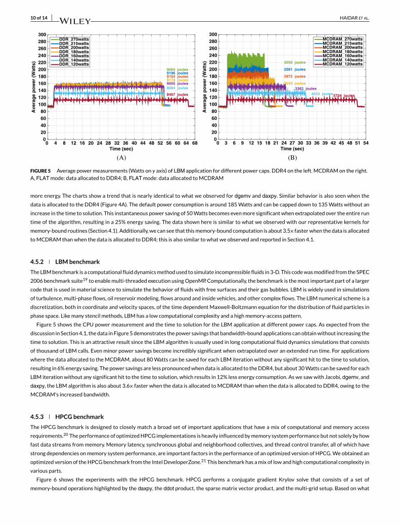
FIGURE 5 Average power measurements (Watts on y axis) of LBM application for different power caps. DDR4 on the left. MCDRAM on the right.A, FLAT mode: data allocated to DDR4; B, FLAT mode: data allocated to MCDRAM
more energy. The charts show a trend that is nearly identical to what we observed for dgemv and daxpy. Similar behavior is also seen when the
data is allocated to the DDR4 (Figure 4A). The default power consumption is around 185 Watts and can be capped down to 135 Watts without an
increase in the time to solution. This instantaneous power saving of 50 Watts becomes even more significant when extrapolated over the entire run
time of the algorithm, resulting in a 25% energy saving. The data shown here is similar to what we observed with our representative kernels for
memory-bound routines (Section 4.1). Additionally, we can see that this memory-bound computation is about 3.5× faster when the data is allocated
to MCDRAM than when the data is allocated to DDR4; this is also similar to what we observed and reported in Section 4.1.
4.5.2 LBM benchmark
The LBM benchmark is a computational fluid dynamics method used to simulate incompressible fluids in 3-D. This code was modified from the SPEC
2006 benchmark suite19 to enable multi-threaded execution using OpenMP. Computationally, the benchmark is the most important part of a larger
code that is used in material science to simulate the behavior of fluids with free surfaces and their gas bubbles. LBM is widely used in simulations
of turbulence, multi-phase flows, oil reservoir modeling, flows around and inside vehicles, and other complex flows. The LBM numerical scheme is a
discretization, both in coordinate and velocity spaces, of the time dependent Maxwell-Boltzmann equation for the distribution of fluid particles in
phase space. Like many stencil methods, LBM has a low computational complexity and a high memory-access pattern.
Figure 5 shows the CPU power measurement and the time to solution for the LBM application at different power caps. As expected from the
discussion in Section 4.1, the data in Figure 5 demonstrates the power savings that bandwidth-bound applications can obtain without increasing the
time to solution. This is an attractive result since the LBM algorithm is usually used in long computational fluid dynamics simulations that consists
of thousand of LBM calls. Even minor power savings become incredibly significant when extrapolated over an extended run time. For applications
where the data allocated to the MCDRAM, about 80 Watts can be saved for each LBM iteration without any significant hit to the time to solution,
resulting in 6% energy saving. The power savings are less pronounced when data is allocated to the DDR4, but about 30 Watts can be saved for each
LBM iteration without any significant hit to the time to solution, which results in 12% less energy consumption. As we saw with Jacobi, dgemv, and
daxpy, the LBM algorithm is also about 3.6× faster when the data is allocated to MCDRAM than when the data is allocated to DDR4, owing to the
MCDRAM's increased bandwidth.
4.5.3 HPCG benchmark
The HPCG benchmark is designed to closely match a broad set of important applications that have a mix of computational and memory access
requirements.20 The performance of optimized HPCG implementations is heavily influenced by memory system performance but not solely by how
fast data streams from memory. Memory latency, synchronous global and neighborhood collectives, and thread control transfer, all of which have
strong dependencies on memory system performance, are important factors in the performance of an optimized version of HPCG. We obtained an
optimized version of the HPCG benchmark from the Intel DeveloperZone.21 This benchmark has a mix of low and high computational complexity in
various parts.
Figure 6 shows the experiments with the HPCG benchmark. HPCG performs a conjugate gradient Krylov solve that consists of a set of
memory-bound operations highlighted by the daxpy, the ddot product, the sparse matrix vector product, and the multi-grid setup. Based on what

HAIDAR ET AL. 11 of 14
Time (sec)0 2 4 6 8 10 12 14 16 18 20 22 24 26 28 30 32 34
Ave
rag
e p
ow
er (
Wat
ts)
020406080
100120140160180200220240260280300
3915 joules3957 joules3940 joules3710 joules3300 joules
3158 joules
DDR_215wattsDDR_200wattsDDR_180wattsDDR_160wattsDDR_140wattsDDR_120watts
(A)
Time (sec)0 2 4 6 8 10 12 14 16 18 20 22 24 26 28 30
Ave
rag
e p
ow
er (
Wat
ts)
020406080
100120140160180200220240260280300
1522 joules1504 joules
1468 joules
1486 joules
1728 joules
2390 joules
MCDRAM_215wattsMCDRAM_200wattsMCDRAM_180wattsMCDRAM_160wattsMCDRAM_140wattsMCDRAM_120watts
(B)
FIGURE 6 Average power measurements (Watts on y axis) of HPCG benchmark on a 192 × 192 × 192 (3-D) grid with varying power caps. DDR4on the left. MCDRAM on the right. A, FLAT mode: data allocated to DDR4; B, FLAT mode: data allocated to MCDRAM
was studied and presented above, one might expect that, with appropriate power caps, applications that use these techniques would see significant
power savings without any negative hit to the time to solution. In fact, Figure 6B shows that a savings of about 30 Watts can be obtained, with the
data allocated to the MCDRAM, while maintaining the same time to solution (5% energy saving). Similarly, Figure 6A shows a savings of 40 Watts,
with the data allocated to DDR4, for a shifted range of power capping levels, which results in approximately 17% less energy consumption.
4.5.4 XSBench mini-app
XSBench represents a key computational kernel of the OpenMC Monte-Carlo neutron transport application. The purpose of this benchmark is to
evaluate the performance of a node's memory subsystem. This is a single-node benchmark that uses OpenMP for node-level parallelism. XSBench
was obtained from the Collaborative Oak Ridge Argonne Livermore (CORAL) benchmark codes website.22 XSBench stresses the system through
memory capacity, random memory access, memory latency, threading, and memory contention, and it is expected to have high memory requirements
and a low computational intensity.
Figure 7 shows a Monte-Carlo neutron transport application characterized by the XSbench suite. In this experiment, we investigated the effect
of our proposed power capping module on a real scientific application. Our results show that significant energy savings can be obtained when using
our power capping technique. In fact, dropping the power cap to around 50-60 Watts below default resulted in a energy savings of roughly 5% for
Time (sec)0 10 20 30 40 50 60 70 80 90 100 110 120 130 140
Ave
rag
e p
ow
er (
Wat
ts)
020406080
100120140160180200220240260280300
19901 joules19796 joules19676 joules17763 joules
16003 joules
13432 joules
DDR_215WattsDDR_200WattsDDR_180WattsDDR_160WattsDDR_140WattsDDR_120Watts
(A)
Time (sec)0 6 12 18 24 30 36 42 48 54 60 66 72 78 84 90 96
Ave
rag
e p
ow
er (
Wat
ts)
020406080
100120140160180200220240260280300
9175 joules8955 joules
8702 joules
8724 joules
10078 joules
MCDRAM_215WattsMCDRAM_200WattsMCDRAM_180WattsMCDRAM_160WattsMCDRAM_140Watts
(B)
FIGURE 7 Average power measurements (Watts on y axis) of XSbench Monte-Carlo neutron transport application for varying power caps. DDR4on the left. MCDRAM on the right. A, FLAT mode: data allocated to DDR4; B, FLAT mode: data allocated to MCDRAM

12 of 14 HAIDAR ET AL.
Time (sec)0 3 6 9 12 15 18 21 24 27 30 33 36 39 42 45 48 51 54
Ave
rag
e p
ow
er (
Wat
ts)
020406080
100120140160180200220240260280300
84 84 84 8484
81
AchievedBandwidth GB/s
Accelerator Power Usage (PACKAGE)Memory Power Usage (DDR4)Max power limit set
MH
z
0 200 400 600 800 100012001400160018002000
Frequency
(A)Time (sec)
0 1 2 3 4 5 6 7 8 9 10111213141516171819202122232425
Ave
rag
e p
ow
er (
Wat
ts)
020406080
100120140160180200220240260280300
392
385
372
316
225
129
AchievedBandwidth GB/s
Accelerator Power Usage (PACKAGE)Memory Power Usage (DDR4)Max power limit set
MH
z
0 200 400 600 800 100012001400160018002000
Frequency
(B)
FIGURE 8 Average power measurements (Watts on y axis) of the Stream benchmark using a vector of size 6.7108 for varying power caps. DDR4on the left. MCDRAM on the right. A, FLAT mode: data allocated to DDR4; B, FLAT mode: data allocated to MCDRAM
MCDRAM and 30% for DDR4. This result confirms that applications with memory-bound workloads can achieve impressive power savings while
maintaining the same time to solution.
4.5.5 Stream benchmark
Stream is a simple synthetic benchmark program designed to measure sustainable memory bandwidth (in MB/s) and the computation rate for simple
vector kernels (ie, copy, scale, add, and triadd).23 As a benchmark, the sustainable memory bandwidth is easy to understand and is likely to be well
correlated with the performance of applications with low computational intensity and limited cache reuse. For our experiments on KNL, we used a
version of Stream that included the Intel-recommended compile optimizations for the KNL architecture.
We evaluated the Stream benchmark23 with a range of power capping levels. For a fixed problem size, the benchmark is called repeatedly; we
capped the power at 20 Watts below default for each call. Figure 8A shows the results obtained during this experiment when the data was allocated
to the DDR4. Figure 8B shows the results obtained when the data was allocated to the MCDRAM. As shown in these graphs, the Stream benchmark
achieves close to the peak bandwidth when running at the default power level. The attainable bandwidth is roughly the same when the power
cap is dropped about 30-40 Watts, regardless of whether the data is allocated to DDR4 or MCDRAM, presenting a significant power savings with
little-to-no performance degradation.
5 RELATED WORK
There are multiple related works that focus on power measurement and the use of power-capping controls for scientific applications. The Power-
Pack project24 provides an interface for measuring power from a variety of external power sources. The API also provides routines for starting and
stopping data collection on the remote machine, and the framework is designed to attribute power consumption to specific devices. PowerPack is
also used to study the efficiency of DVFS.
Global Extensible Open Power Manager (GEOPM)25 is a power management framework targeting high-performance computing that is designed
to be extended using plugins that implement new algorithms and features. Power information is queried via Model Specific Registers (MSRs), and
control policy is also applied via the MSRs. An example plugin manages a power budget for a whole system, minimizing the time-to-solution while
remaining within the power budget.
The READEX (Run-time Exploitation of Application Dynamism for Energy-efficient Exascale computing) project26,27 is a EU Horizon 2020 effort
that is creating tools to achieve efficient execution on Exascale systems. These tools use automatic analysis to identify dynamism in an application,
then a lightweight runtime library is used to perform runtime tuning actions during the application's execution.
Adagio is a runtime system that makes dynamic voltage scaling (DVS) practical for complex scientific applications.28 Adagio shares our goal
of incurring negligible penalty to an application's time to solution while achieving energy savings. This is accomplished by using a history-based
scheduling mechanism that executes tasks at different power caps (DVS) based on the “energy slack” observed in previous executions.
Kimura et al29 examine slack in unbalanced work distributions generated from distributed DAG executions and use DVFS to adapt the exe-
cution speed for tasks in order to balance the execution without increasing the overall execution time. Bhalachandra et al30 use several system
metrics (eg, TOR Table-Of-Requests occupancy) to characterize memory behavior and apply coarse-grained and fine-grained power policies
HAIDAR ET AL. 13 of 14
implemented using DVFS. They demonstrate substantial power savings on mini-apps with minimal performance change using these system metrics.
Porterfield et al31 present experiments on distributed memory applications, enforcing power limits from within MPI communication libraries when
collective operations are occurring. This approach is capable of saving energy for large-scale applications with minimal costs to execution time.
Additionally, the Linux kernel has begun to expose RAPL-based power management via the sysfs powercap interface, which provides simpler
and safer access to the low-level power controls. The Linux perf command-line interface has begun exposing and managing some of the hardware
counters, but the power management is still handled by accessing the sysfs powercap file system.
Finally, there's PUPiL,32 which is a hardware/software power capping framework that uses hardware controls like DVS in combination with flex-
ible software to enable capping in applications in such a way that PUPiL can be considered a replacement for RAPL as a transparent power-capping
framework.
6 CONCLUSION
Designing numerical libraries and scientific applications with energy consumption as a primary constraint presents significant challenges for devel-
opers. This paper presents results of a study where PAPI's new power control functionality was used to limit the power consumption in a set of
representative kernels on the Intel KNL computing platform. PAPI's new powercap component extends the current PAPI interface from a passive
read-only interface to an active interface that allows writing values in addition to reading them. This means that users and third-party tools need only
a single hook to PAPI in order to access any hardware performance counters across a system, including the new power-capping functionality.
This paper demonstrates how PAPI enables power tuning to reduce overall energy consumption without, in many cases, a loss in performance. We
present a detailed analysis of the performance of different kernels and the power consumption of various hardware components when subjected to
a range of power caps. The kernels in these experiments were chosen not only because they represent a significant fraction of real-world scientific
workloads but also because they have different computation-to-memory-traffic ratios. All experiments were performed on KNL configured in flat
mode (ie, the MCDRAM is used as addressable memory), and for each case, studies were performed with data allocated to the MCDRAM and to
the DDR4.
Our experiments show that, depending on the computational density of the kernel and the speed of the memory used to store the data, the power
consumption of some of these kernels could be limited using PAPI in ways that led to an overall reduction of energy consumption (up to 30%) without
reducing the performance of the kernel. This demonstrates that the usefulness of the powercap component, which allows applications to control
the power limit of the hardware, is not only theoretical but can be used in the libraries and kernels that will drive the software stack of tomorrow's
supercomputers.
ACKNOWLEDGMENTS
This material is based upon work supported in part by the National Science Foundation NSF under grants 1450429 “Performance Application
Programming Interface for Extreme-scale Environments (PAPI-EX)” and grant 1514286. A portion of this research was supported by the Exascale
Computing Project (17-SC-20-SC), a collaborative effort of the U.S. Department of Energy Office of Science and the National Nuclear Security
Administration.
ORCID
Azzam Haidar http://orcid.org/0000-0002-3177-2084
Heike Jagode http://orcid.org/0000-0002-8173-9434
REFERENCES
1. Rotem E, Naveh A, Ananthakrishnan A, Weissmann E, Rajwan D. Power-management architecture of the Intel microarchitecture code-named SandyBridge. IEEE Micro. 2012;32(2):20-27.
2. Le Sueur E, Heiser G. Dynamic voltage and frequency scaling: The laws of diminishing returns. Paper presented at: International Conference on PowerAware Computing and Systems; 2010; Berkeley, CA.
3. Terpstra D, Jagode H, You H, Dongarra J. Collecting Performance Data with PAPI-C. Paper presented at: International Workshop on Parallel Tools forHigh Performance Computing; 2009; Dresden, Germany.
4. Malony AD, Biersdorff S, Shende S, et al. Parallel performance measurement of heterogeneous parallel systems with GPUs. Paper presented at:International Conference on Parallel Processing; 2011; Washington, DC.
5. McCraw H, Terpstra D, Dongarra J, Davis KRM. Beyond the CPU: Hardware performance counter monitoring on blue Gene/Q. Paper presented at:International Supercomputing Conference; 2013; Leipzig, Germany.
6. Cray Inc. Using the PAPI Cray NPU Component. 2013. http://docs.cray.com/books/S-0046-10//S-0046-10.pdf

14 of 14 HAIDAR ET AL.
7. McCraw H, Ralph J, Danalis A, Dongarra J. Power monitoring with PAPI for extreme scale architectures and dataflow-based programming models. Paperpresented at: Workshop on Monitoring and Analysis for High Performance Computing Systems Plus Applications; 2014; Madrid, Spain.
8. Jagode H, Yar Khan A, Danalis A, Dongarra J. Power Management and Event Verification in PAPI. Paper presented at: 9th International Workshop onParallel Tools for High Performance Computing; 2016; Dresden, Germany.
9. Johnson M, Jagode H, Moore S, et al. PAPI-V: Performance monitoring for virtual machines. Paper presented at: CloudTech-HPC Workshop; 2012;Pittsburgh, PA.
10. Cray Inc. The CrayPat performance analysis tool. http://docs.cray.com/books/S-2315-50/html-S-2315-50/z1055157958smg.html
11. Adhianto L, Banerjee S, Fagan M, et al. HPCTOOLKIT: tools for performance analysis of optimized parallel programs. Concurr Comput Pract Exp.2010;22(6):685-701.
12. Geimer M, Wolf F, Wylie BJN, Ábrahám E, Becker D, Mohr B. The Scalasca performance toolset architecture. Concurr Comput Pract Exp.2010;22(6):702-719.
13. Schlütter M, Philippen P, Morin L, Geimer M, Mohr B. Profiling hybrid HMPP applications with Score-P on heterogeneous hardware. In: Bader M,Bode A, Bungartz HJ, Gerndt M, Joubert G, Peters F, eds. Parallel Computing: Accelerating Computational Science and Engineering (CSE). IOS Press:Amsterdam, Netherlands; 2014:773-782. Advances in Parallel Computing; vol 25. https://doi.org/10.3233/978-1-61499-381-0-773
14. Shende SS, Malony AD. The tau parallel performance system. Int J High Perform Comput Appl. 2006;20(2):287-311.
15. Brunst H, Knüpfer A. Vampir. In: Padua D, ed. Encyclopedia of Parallel Computing. New York, NY: Springer; 2011:2125-2129. https://doi.org/10.1007/978-0-387-09766-4_60
16. Burtscher M, Kim BD, Diamond J, McCalpin J, Koesterke L, Browne J. PerfExpert: An easy-to-use performance diagnosis tool for HPC applications. Paperpresented at: ACM/IEEE International Conference for High Performance Computing, Networking, Storage and Analysis; 2010; Washington, DC
17. Lucas R, Ang J, Bergman K, et al. Top ten exascale research challenges. DOE ASCAC Subcommittee Report; 2014.
18. Intel Corporation. Intel. Intel 64 and IA-32 Architectures Software Developer's Manual Volume 3B: System Programming Guide, Part 2. 2016. https://www.intel.com/content/dam/www/public/us/en/documents/manuals/64-ia-32-architectures-software-developer-vol-3b-part-2-manual.pdf
19. Henning JL. Spec CPU2006 Benchmark Descriptions. ACM SIGARCH Comput Archit News. 2006;34(4):1-17.
20. Dongarra J, Heroux MA, Luszczek P. High-performance conjugate-gradient benchmark: a new metric for ranking high-performance computing systems.Int J High Perform Comput Appl. 2016;30(1):3-10.
21. Intel Corporation. Intel I. Intel Math Kernel Library Benchmarks (Intel® MKL Benchmarks). https://software.intel.com/en-us/articles/intel-mkl-benchmarks-suite
22. Laboratory LLN. Coral benchmark code collection. https://asc.llnl.gov/CORAL-benchmarks/
23. McCalpin J. Stream: Measuring sustainable memory bandwidth in high performance computers. 1996. http://www.cs.virginia.edu/stream
24. Ge R, Feng X, Song S, Chang HC, Li D, Cameron KW. Powerpack: energy profiling and analysis of high-performance systems and applications. IEEE TransParallel Distributed Syst. 2010;21(5):658-671.
25. Eastep J, Sylvester S, Cantalupo C, et al. Global Extensible Open Power Manager: A Vehicle for HPC Community Collaboration on Co-Designed EnergyManagement Solutions. Cham, Switzerland: Springer International Publishing; 2017;394-412. https://doi.org/10.1007/978-3-319-58667-0_21
26. Schuchart J, Gerndt M, Kjeldsberg PG, et al. The READEX formalism for automatic tuning for energy efficiency. Computing. 2017;99(8):727-745.
27. Oleynik Y, Gerndt M, Schuchart J, Kjeldsberg PG, Nagel WE. Run-time exploitation of application dynamism for energy-efficient exascale computing(readex). Paper presented at: 18th International Conference on Computational Science and Engineering; 2015; Porto, Portugal.
28. Rountree B, Lownenthal DK, de Supinski BR, Schulz M, Freeh VW, Bletsch T. Adagio: Making DVS practical for complex HPC applications. Paper presentedat: 23rd International Conference on Supercomputing; 2009; Yorktown Heights, NY.
29. Kimura H, Sato M, Hotta Y, Boku T, Takahashi D. Empirical study on reducing energy of parallel programs using slack reclamation by DVFS in apower-scalable high performance cluster. Paper presented at: 2006 IEEE International Conference on Cluster Computing; 2006; Barcelona, Spain.
30. Bhalachandra S, Porterfield A, Olivier SL, Prins JF, Fowler RJ. Improving energy efficiency in memory-constrained applications using core-specific powercontrol. Paper presented at: 5th International Workshop on Energy Efficient Supercomputing; 2017; Denver, CO.
31. Porterfield A, Fowler R, Bhalachandra S, Rountree B, Deb D, Lewis R. Application runtime variability and power optimization for exascale computers.Paper presented at: 5th International Workshop on Runtime and Operating Systems for Supercomputers; 2015; Portland, OR.
32. Zhang H, Hoffmann H. Maximizing performance under a power cap: A comparison of hardware, software, and hybrid techniques. Paper presented at:21st International Conference on Architectural Support for Programming Languages and Operating Systems; 2016; Atlanta, GA.
How to cite this article: Haidar A, Jagode H, Vaccaro P, YarKhan A, Tomov S, Dongarra J. Investigating power capping toward
energy-efficient scientific applications. Concurrency Computat Pract Exper. 2018;e4485. https://doi.org/10.1002/cpe.4485