investigating key techniques to leverage the functionality

University of VermontScholarWorks @ UVM

Graduate College Dissertations and Theses Dissertations and Theses

2017

Investigating Key Techniques to Leverage theFunctionality of Ground/Wall Penetrating RadarYu ZhangUniversity of Vermont

Follow this and additional works at: https://scholarworks.uvm.edu/graddis

Part of the Electrical and Electronics Commons

This Dissertation is brought to you for free and open access by the Dissertations and Theses at ScholarWorks @ UVM. It has been accepted forinclusion in Graduate College Dissertations and Theses by an authorized administrator of ScholarWorks @ UVM. For more information, please [email protected].

Recommended CitationZhang, Yu, "Investigating Key Techniques to Leverage the Functionality of Ground/Wall Penetrating Radar" (2017). Graduate CollegeDissertations and Theses. 799.https://scholarworks.uvm.edu/graddis/799

https://scholarworks.uvm.edu?utm_source=scholarworks.uvm.edu%2Fgraddis%2F799&utm_medium=PDF&utm_campaign=PDFCoverPages

https://scholarworks.uvm.edu/graddis?utm_source=scholarworks.uvm.edu%2Fgraddis%2F799&utm_medium=PDF&utm_campaign=PDFCoverPages

https://scholarworks.uvm.edu/etds?utm_source=scholarworks.uvm.edu%2Fgraddis%2F799&utm_medium=PDF&utm_campaign=PDFCoverPages

https://scholarworks.uvm.edu/graddis?utm_source=scholarworks.uvm.edu%2Fgraddis%2F799&utm_medium=PDF&utm_campaign=PDFCoverPages

http://network.bepress.com/hgg/discipline/270?utm_source=scholarworks.uvm.edu%2Fgraddis%2F799&utm_medium=PDF&utm_campaign=PDFCoverPages

https://scholarworks.uvm.edu/graddis/799?utm_source=scholarworks.uvm.edu%2Fgraddis%2F799&utm_medium=PDF&utm_campaign=PDFCoverPages

mailto:[email protected]

INVESTIGATING KEY TECHNIQUES TO LEVERAGE THE FUNCTIONALITY OF

GROUND/WALL PENETRATING RADAR

A Dissertation Presented

by

Yu Zhang

to

The Faculty of the Graduate College

of

The University of Vermont

In Partial Fulfillment of the Requirements

for the Degree of Doctor of Philosophy

Specializing in Electrical Engineering

October, 2017

Defense Date: August 14, 2017

Dissertation Examination Committee:

Tian Xia, Ph.D., Advisor

Dryver R. Huston, Ph.D., Chairperson

Kurt E. Oughstun, Ph.D.

Mads R. Almassalkhi, Ph.D.

Cynthia J. Forehand, Ph.D., Dean of the Graduate College

ABSTRACT

Ground penetrating radar (GPR) has been extensively utilized as a highly efficient

and non-destructive testing method for infrastructure evaluation, such as highway rebar

detection, bridge decks inspection, asphalt pavement monitoring, underground pipe

leakage detection, railroad ballast assessment, etc. The focus of this dissertation is to

investigate the key techniques to tackle with GPR signal processing from three

perspectives: (1) Removing or suppressing the radar clutter signal; (2) Detecting the

underground target or the region of interest (RoI) in the GPR image; (3) Imaging the

underground target to eliminate or alleviate the feature distortion and reconstructing the

shape of the target with good fidelity.

In the first part of this dissertation, a low-rank and sparse representation based

approach is designed to remove the clutter produced by rough ground surface reflection

for impulse radar. In the second part, Hilbert Transform and 2-D Renyi entropy based

statistical analysis is explored to improve RoI detection efficiency and to reduce the

computational cost for more sophisticated data post-processing. In the third part, a back-

projection imaging algorithm is designed for both ground-coupled and air-coupled

multistatic GPR configurations. Since the refraction phenomenon at the air-ground

interface is considered and the spatial offsets between the transceiver antennas are

compensated in this algorithm, the data points collected by receiver antennas in time

domain can be accurately mapped back to the spatial domain and the targets can be

imaged in the scene space under testing. Experimental results validate that the proposed

three-stage cascade signal processing methodologies can improve the performance of

GPR system.

ii

CITATIONS

Material from this dissertation has been published in the following form:

Zhang, Y. and Xia, T.. (2016). In-Wall Clutter Suppression based on Low-Rank and

Sparse Representation for Through-the-Wall Radar. IEEE Geoscience and Remote

Sensing Letters, 13(5), 671-675.

Zhang, Y., Venkatachalam, A. S. and Xia, T.. (2015). Ground-penetrating radar

railroad ballast inspection with an unsupervised algorithm to boost the region of interest

detection efficiency. SPIE Journal of Applied Remote Sensing, 9(1), 1-19.

Zhang, Y., Candra, P., Wang, G. and Xia, T.. (2015). 2-D Entropy and Short-Time

Fourier Transform to Leverage GPR Data Analysis Efficiency. IEEE Transactions on

Instrumentation and Measurement, 64(1), 103-111.

AND

Material from this dissertation has been submitted for publication to IEEE Transactions

on Geoscience and Remote Sensing on August 07, 2017 in the following form:

Zhang, Y., Burns, D., Orfeo, D., Huston, D. and Xia, T.. Air Coupled Ground

Penetrating Radar Clutter Mitigation for Rough Surface Sensing. IEEE Transactions on

Geoscience and Remote Sensing.

iii

ACKNOWLEDGEMENTS

First, I would like to express my deepest gratitude to my PhD advisor, Dr. Tian Xia.

For the past five years, he has been not only an advisor in research, but also a mentor

and a good friend in life. Without his generous mentorship, guidance, encouragement

and support, I could not achieve so much. His inexhaustible passion in research and

dedication to students have set up an inspirational model for me.

Second, a special thanks to Dr. Dryver Huston, my co-advisor and committee

chairperson, for his continuous guidance and insightful suggestions during our five

years’ collaborative research. I can always learn great ideas from him on our group

meeting every Friday morning. I would like to extend my gratitude to my dissertation

committee, Dr. Kurt Oughstun and Dr. Mads Almassalkhi, for their precious time in

reviewing my dissertation and their valuable suggestions. I would also like to thank Dr.

Gagan Mirchandani, for serving on my PhD comprehensive exam committee and

teaching the philosophy of matrix theory in his course. I would also like to thank Dr.

Yuanchang Xie, for his help on our collaborative research and GPR field testing in

Summer 2013.

Third, I would like to thank my colleagues, especially Dr. Dylan Burns, Dan Orfeo,

Wenzhe Chen, Lixi Tao, Amr Ahmed, and Taian Fan. Thank you for all the help and

friendship during my five years’ PhD journey. A special thanks to Anbu

Venkatachalam, the best officemate, badminton partner and friend for generous help on

iv

both research and life when I was a freshman at UVM. Again, to all my colleagues, it

was an honor working with all of you at UVM and I really hope that our roads will

cross again in future.

Fourth, I would like to express my gratitude to the people who offered their help during

my job-hunting period. Thanks to Mr. John Carulli for his “tips & tricks” on preparing

the resume and insightful suggestions on choosing career path from the perspective of a

UVM alumni. Thanks to Dr. Hamid Ossareh for his insightful advices on negotiating

the job offer in automotive industry.

Fifth, I would like to thank the staff members of the College of Engineering and

Mathematical Sciences, especially Karen Bernard, Katarina Khosravi, Pattie McNatt,

and Sharon Sylvester, and the staff members of Graduate College, especially Kimberly

Hess, Sean Milnamow and Bethany Sheldon, for all the help they provided over these

years.

Finally, I would love to thank my parents. Their unconditional love and support are

invaluable to me. I am proud to be their son. I would also express my deep gratitude to

my girlfriend, Dr. Tianxin Miao, who is going to be another Dr. Zhang soon. We built

our first home together at UVM Apartment Family Housing with all our plush animal

friends. She has been giving me bottomless love and infinite tolerance of my increasing

collection of transformer action figures.

v

TABLE OF CONTENTS

Page

ACKNOWLEDGEMENTS ............................................................................................ iii

LIST OF TABLES ........................................................................................................... x

LIST OF FIGURES ........................................................................................................ xi

CHAPTER 1: INTRODUCTION .................................................................................... 1

1.1. Non-destructive Testing Problem .......................................................................... 1

1.2. Background of Ground Penetrating Radar ............................................................ 3

1.2.1. History and Applications .................................................................................. 3

1.2.2. Operating Mechanism ....................................................................................... 5

1.2.3. System Architecture: Impulse Radar, SFCW Radar and FMCW Radar .......... 7

1.2.4. Height of Antenna: Ground-Coupled GPR and Air-Coupled GPR ................ 10

1.2.5. Spatial Offset between Antennas: Monostatic, Bistatic and Multistatic ........ 11

1.2.6. Critical Specifications ..................................................................................... 12

1.3. GPR Signal Processing Problems and Methodologies ........................................ 15

1.3.1. Trace Editing and Rubber-banding ................................................................. 15

1.3.2. Dewow ............................................................................................................ 16

1.3.3. Time-zero correction ...................................................................................... 17

1.3.4. Range Filtering and Cross-Range Filtering .................................................... 17

1.3.5. Deconvolution ................................................................................................. 20

1.3.6. Migration ........................................................................................................ 20

1.3.7. Attribute Analysis ........................................................................................... 24

1.3.8. Gain Adjustment ............................................................................................. 25

1.3.9. Image analysis ................................................................................................ 27

1.3.10. Region of Interest Detection ......................................................................... 28

vi

1.3.11. Summary ....................................................................................................... 28

1.4. Objective and Scope ............................................................................................ 29

1.5. References............................................................................................................ 31

CHAPTER 2: IN-WALL CLUTTER SUPPRESSION BASED ON LOW-

RANK AND SPARSE REPRESENTATION FOR THROUGH-THE-WALL

RADAR.......................................................................................................................... 45

Abstract ....................................................................................................................... 45

2.1. Introduction ......................................................................................................... 45

2.2. Low-Rank and Sparse Representation ................................................................. 49

2.3. In-Wall Clutter Suppression for See-through-wall Radar ................................... 50

2.4. Experimental results ............................................................................................ 53

2.4.1. Experiment with the Synthetic Data ............................................................... 53

2.4.2. Experiment with the Field Test Data .............................................................. 56

2.5. Conclusions ......................................................................................................... 60

2.6. References............................................................................................................ 60

CHAPTER 3: AIR COUPLED GROUND PENETRATING RADAR

CLUTTER MITIGATION FOR ROUGH SURFACE SENSING ................................ 63

Abstract ....................................................................................................................... 63

3.1. Introduction ......................................................................................................... 63

3.2. GPR B-Scan Image Model .................................................................................. 66

3.3. Low-Rank and Sparse Decomposition Based Clutter Removal .......................... 68

vii

3.4. Experimental results ............................................................................................ 72

3.4.1. Simulation Data 1: Oblique Ground Surface .................................................. 72

3.4.2. Simulation Data 2: Rough Ground Surface .................................................... 75

3.4.3. Experiment with Lab Test Data ...................................................................... 78

3.4.4. Quantitative Analysis on the Processed Data ................................................. 80

3.5. Conclusions ......................................................................................................... 81

3.6. References............................................................................................................ 81

CHAPTER 4: 2-D ENTROPY AND SHORT-TIME FOURIER TRANSFORM

TO LEVERAGE GPR DATA ANALYSIS EFFICIENCY .......................................... 84

Abstract ....................................................................................................................... 84

4.1. Introduction ......................................................................................................... 84

4.2. Data Acquisition .................................................................................................. 88

4.2.1. System Setup .................................................................................................. 88

4.2.2. Test Setups ...................................................................................................... 89

4.2.3. GPR Data Pre-Processing ............................................................................... 91

4.3. Computational algorithms: 2-D Entropy and Short-Time Fourier

Transform ................................................................................................................... 93

4.3.1. Windowing 2D Entropy Method .................................................................... 93

4.3.2. Entropy Curve Smoothing Using Moving Average ....................................... 96

4.3.3. Adaptive Entropy Threshold Determination .................................................. 96

4.3.4. Short Time Fourier Transform (STFT) ........................................................... 99

4.4. Experiment Results and Discussion..................................................................... 99

4.4.1. Rebar Test Results .......................................................................................... 99

4.4.2. Ballast Test Results ....................................................................................... 108

viii

4.5. Conclusions ....................................................................................................... 111

4.6. References.......................................................................................................... 112

CHAPTER 5: GROUND PENETRATING RADAR RAILROAD BALLAST

INSPECTION WITH AN UNSUPERVISED ALGORITHM TO BOOST THE

REGION OF INTEREST DETECTION EFFICIENCY ............................................. 114

Abstract ..................................................................................................................... 114

5.1. Introduction ....................................................................................................... 115

5.2. GPR System Configuration ............................................................................... 118

5.3. Unsupervised GPR ROI Detection Method ....................................................... 120

5.3.1. Pre-processing ............................................................................................... 120

5.3.2. Power Information Characterization ............................................................. 122

5.3.3. Identification of Ballast Region .................................................................... 123

5.3.4. B-Scan Image Enhancement ......................................................................... 125

5.3.5. Entropy Based Region of Interest (ROI) Detection ...................................... 125

5.4. Lab Experiment ................................................................................................. 128

5.4.1. Test Configuration ........................................................................................ 128

5.4.2. ROI Detection ............................................................................................... 129

5.5. Inspection of Railroad Ballast ........................................................................... 133

5.5.1. Test Configuration ........................................................................................ 133

5.5.2. ROI Detection ............................................................................................... 136

5.6. Discussion and Conclusions .............................................................................. 139

5.7. References.......................................................................................................... 140

ix

CHAPTER 6: MULTISTATIC GROUND PENETRATING RADAR

IMAGING USING BACK-PROJECTION ALGORITHM ........................................ 142

6.1. Introduction ....................................................................................................... 142

6.2. Stolt Migration Algorithm and Back-Projection Algorithm .............................. 144

6.2.1. SMA for Ground-Coupled Monostatic GPR ................................................ 144

6.2.2. Improved SMA for Ground-Coupled Bistatic GPR ..................................... 147

6.2.3. BPA for Ground-Coupled Monostatic GPR ................................................. 152

6.2.4. Comparison between SMA and BPA ........................................................... 158

6.3. Ground-Coupled Multistatic GPR Imaging Methodology ................................ 160

6.3.1. System Configuration ................................................................................... 160

6.3.2. BPA for Ground-Coupled Multistatic GPR Imaging ................................... 161

6.4. Air-Coupled Multistatic GPR Imaging Methodology ....................................... 165

6.5. Experimental Results ......................................................................................... 171

6.5.1. Ground-Coupled GPR Imaging Experiments ............................................... 171

6.5.2. Air-Coupled GPR Imaging Experiments ...................................................... 179

6.6. Conclusions ....................................................................................................... 182

6.7. References.......................................................................................................... 182

CHAPTER 7: CONCLUSIONS AND FUTURE WORKS ......................................... 185

7.1. Conclusions ....................................................................................................... 185

7.2. Future Work ....................................................................................................... 185

7.3. References.......................................................................................................... 187

BIBLIOGRAPHY ........................................................................................................ 189

x

LIST OF TABLES

Table Page

Table 1.1: Antenna frequency, approximate depth penetration and appropriate

application [66]. ............................................................................................................. 14

Table 3.1: SCR of each B-Scan Image. ......................................................................... 80

Table 5.1: Air-coupled Impulse GPR System Specifications. ..................................... 119

Table 5.2: Key Parameters Used in the GPR Field Tests. ........................................... 133

xi

LIST OF FIGURES

Figure Page

Figure 1.1: GPR explored in various case studies for non-destructive

underground infrastructure inspection: (a) asphalt pavement inspection; (b)

bridge deck inspection [19]; (c) rebar detection; (d) underground utilities

mapping for smart city; (e) railroad ballast condition assessment. .................................. 3

Figure 1.2: Model depicting the various scattered signals in impulse ground

penetrating radar and the scattered signals shown in time domain [56] .......................... 6

Figure 1.3: Block diagram of basic impulse GPR system [57]. ...................................... 8

Figure 1.4: Block diagram of SFCW radar system [58]. ................................................. 8

Figure 1.5: Simplified block diagram of a coherent linear FMCW radar system

[57]. .................................................................................................................................. 9

Figure 1.6: GPR antenna configuration: (a) GSSI SIR-30 ground-coupled GPR

system; (b) UVM air-coupled impulse GPR system. ..................................................... 10

Figure 1.7: Antenna configuration of monostatic GPR, bistatic GPR and

multistatic GPR. ............................................................................................................. 12

Figure 1.8: Hyperbolic distortion in GPR image: (a) geometrical layout of GPR

inspection; (b) hyperbolic distortion in GPR B-Scan image [112]. ............................... 21

Figure 2.1: TWR imaging scenario ................................................................................ 51

Figure 2.2: Synthetic data: (a) Geometry structure; (2) Raw TWR image. ................... 54

Figure 2.3: Processed synthetic data: (a) Pre-processing – stationary background

removal; (b) In-wall clutter removal with low-rank and sparse representation

technique. ....................................................................................................................... 55

Figure 2.4: Processed simulation data using pattern matching. ..................................... 56

Figure 2.5: Field test data: (a) A hard disk attached on the wall; (b) TWR

scanning from the other side of the wall; (c) MALA concrete imaging system;

(d) Raw TWR image. ..................................................................................................... 57

xii

Figure 2.6: Processed field test data: (a) Pre-processing – stationary background

removal; (b) In-wall clutter suppression. ....................................................................... 58

Figure 2.7: Processed field test data using pattern matching. ........................................ 59

Figure 3.1: Ground clutter removal process .................................................................. 71

Figure 3.2: Synthetized oblique ground surface: (a) Geometry data; (b) Raw B-

scan image; (c) Average subtraction from raw B-Scan. ................................................ 74

Figure 3.3: Synthesized oblique ground surface: A-Scan trace at various

locations along scan axis. ............................................................................................... 74

Figure 3.4: Synthetic oblique ground surface: (a) Aligned B-Scan; (b) Clutter

removal using average subtraction; (c) Clutter removal using proposed method. ........ 75

Figure 3.5: Synthetic rough ground surface: (a) Geometry data; (b) Raw B-scan

image; (c) Average subtraction from raw B-Scan. ........................................................ 76

Figure 3.6: Synthesized rough ground surface: A-Scan trace at various locations

along scan axis. .............................................................................................................. 77

Figure 3.7: Synthetic rough ground surface: (a) Aligned B-Scan; (b) Clutter

removal using average subtraction; (c) Clutter removal using the proposed

method............................................................................................................................ 77

Figure 3.8: Lab sandbox test: (a) Geometry data; (b) Raw B-scan image; (c)

Average subtraction from raw B-Scan. .......................................................................... 79

Figure 3.9: Lab sandbox test: (a) Aligned B-Scan; (b) Clutter removal using

average subtraction; (c) Clutter removal using the proposed method. .......................... 79

Figure 4.1: GPR system diagram: (a) High Speed UWB GPR System; (b) UWB

Pulse Generator; (c) UWB Horn Antenna; (d) Reflection Loss of the UWB

Horn Antenna. ................................................................................................................ 89

Figure 4.2: Measurement setup (a) rebar in air; (b) rebar in concrete; (c) Two

horn antennas. ................................................................................................................ 90

Figure 4.3: Ballast Test Configuration: (a) Test Platform; (b) Subsurface

Construction. .................................................................................................................. 91

Figure 4.4: Raw B-scan images of (a) rebar in air; (b) Two rebars in a concrete

slab. ................................................................................................................................ 91

xiii

Figure 4.5: Rebar-in-Air B-scan images after preprocessing: (a) Reference trace

subtraction and a LPF filtering; (b) Reference trace subtraction, LPF filtering

and trace averaging operations. ...................................................................................... 92

Figure 4.6: B-Scan images for ballast setup: (a) Raw B-Scan image; (b) B-Scan

image upon preprocessing.............................................................................................. 93

Figure 4.7: Pulse peak point shift on different trace index = 1000, 1200, 1400,

1600, 1800, 2000, 2200.................................................................................................. 95

Figure 4.8: Entropy data of One Rebar in Air B-Scan. .................................................. 96

Figure 4.9: Entropy analysis along pulse time index (Y-axis) of rebar in-air data:

(a) B-Scan image; (b) Entropy data. ............................................................................ 101

Figure 4.10: Entropy analysis along trace index (X-axis) of rebar in air B-scan:

(a) B-Scan image; (b) Entropy data. ............................................................................ 102

Figure 4.11: 2D entropy analysis for B-scan images of a) rebar in air and b)

rebars in concrete. ........................................................................................................ 103

Figure 4.12: STFT analysis to correct the singular region detection: (a) STFT

result of one rebar data at x=1.1m; (b) STFT result of two rebar data at x=1.5m. ...... 104

Figure 4.13: Final singular region for B-scan images of a) rebar in air and b)

two rebars in concrete. ................................................................................................. 104

Figure 4.14: (a) Rebar in air B-scan image; 2D entropy and STFT analysis

results of traces at (b) left side, (c) middle and (d) right side of rebar area. ................ 105

Figure 4.15: (a) Rebars in concrete B-scan image; 2D entropy and STFT

analysis at (b) left rebar and (c) right rebar. ................................................................. 107

Figure 4.16: Entropy analysis of ballast data: (a) Entropy along Travel time

index (Y-axis); (b) Entropy along Scan Axis (X-axis). ............................................... 108

Figure 4.17: 2-D entropy analysis for B-Scan image of ballast platform. ................... 109

Figure 4.18: STFT analysis result of trace at x = 2.5 m. ............................................. 110

Figure 4.19: Final moisture region detection result based on entropy and STFT

analysis. ........................................................................................................................ 110

Figure 5.1: GPR system diagram: (a) High Speed UWB GPR System; (b)

Digitizer Configured in SAR Mode; (c) UWB Pulse Generator; (d) UWB

Antenna. ....................................................................................................................... 118

xiv

Figure 5.2: Unsupervised algorithm for detecting region of interest in ballast

layer.............................................................................................................................. 120

Figure 5.3: Amplitude spectrum of GPR A-Scan trace. .............................................. 121

Figure 5.4: Hilbert transform for signal power characterization: (a) GPR A-Scan

trace; (b) GPR A-Scan envelope. ................................................................................. 123

Figure 5.5: Signal decomposition for identification of backscattering from

different sources: (a) Direct coupling signal; (b) 1st backscattering pulse; (c)

2nd backscattering pulse. ............................................................................................. 125

Figure 5.6: Railroad ballast lab test configuration: (a) Test platform; (b)

Subsurface structure. .................................................................................................... 128

Figure 5.7: B-Scan image from lab tests: (a) Raw B-Scan image; (b) Pre-

processed B-Scan image. ............................................................................................. 129

Figure 5.8: Signal Magnitude Characterization through Hilbert Transform: (a)

B-Scan image plotted using signal magnitude data; (b) Systematic background

signals identified through decomposition method; (c) A sample A-Scan trace

waveform. .................................................................................................................... 130

Figure 5.9: B-Scan image for ballast layer: (a) Ballast layer; (b) Enhanced

ballast layer. ................................................................................................................. 131

Figure 5.10: Entropy analysis of ballast data of Figure 5.8(b): (a) Entropy along

Travel time index (y-axis); (b) Entropy along Scan Axis (x-axis). ............................. 132

Figure 5.11: 2D entropy analysis of the B-Scan image collected from the test

platform. ....................................................................................................................... 132

Figure 5.12: GPR System configuration during field tests. ......................................... 134

Figure 5.13: Site pictures: (a) Metro St. Louis MetroLink Blue line; (b) Railroad

ballast. .......................................................................................................................... 135

Figure 5.14: (a) Field test raw B-Scan image; (b) Pre-processed B-Scan image. ....... 136

Figure 5.15: (a) Field test B-Scan image obtained from signal magnitude ; (b)

cross-tie marked by signal decomposition; (c) A-Scan signal at x = 3.8 m................. 136

Figure 5.16: B-Scan image for ballast layer: (a) Ballast layer; (b) Enhanced

ballast layer. ................................................................................................................. 137

xv

Figure 5.17: Entropy analysis of ballast data of Figure 5.15(b) along: (a) Travel

time axis and (b) Scan Distance axis. .......................................................................... 138

Figure 5.18: Automatic suspicious fouled ballast regions marked by white

rectangle. ...................................................................................................................... 139

Figure 6.1: One pair of transceiver antennas in multi-static GPR configuration. ........ 148

Figure 6.2: WST-SMA Migration Flow Chart. ........................................................... 151

Figure 6.3: Principle of BPA for monostatic GPR: (a) Distance between antenna

and target in scene space; (b) Wave propagating time from antenna to target; (c)

Time domain data points back projected to scene space. ............................................ 152

Figure 6.4: Implementation of BPA for ground-coupled monostatic GPR ................. 154

Figure 6.5: Ground-coupled multistatic GPR configuration. ....................................... 161

Figure 6.6: Ground-coupled multistatic GPR imaging. ............................................... 162

Figure 6.7: Air-coupled multistatic GPR configuration. ............................................. 165

Figure 6.8: Air-coupled multistatic GPR imaging. ...................................................... 166

Figure 6.9: Ground-coupled multistatic GPR testing setup – three buried targets. ..... 172

Figure 6.10: Ground-coupled multistatic GPR raw B-Scan – three buried

targets: (1) Tx1-Rx1 pair; (2) Tx1-Rx5 pair. ............................................................... 173

Figure 6.11: Ground-coupled multistatic GPR migrated B-Scan – three buried

targets: (1) Tx1-Rx1 pair; (2) Tx1-Rx5 pair. ............................................................... 174

Figure 6.12: Ground-coupled multistatic GPR migrated B-Scan using proposed

multistatic imaging method – three buried targets ....................................................... 175

Figure 6.13: Ground-coupled multistatic GPR testing setup – three buried

targets. .......................................................................................................................... 176

Figure 6.14: Ground-coupled multistatic GPR raw B-Scan – congested pipes:

(1) Tx1-Rx1 pair; (2) Tx1-Rx5 pair. ............................................................................ 177

Figure 6.15: Ground-coupled multistatic GPR migrated B-Scan – congested

pipes: (1) Tx1-Rx1 pair; (2) Tx1-Rx5 pair. ................................................................. 178

Figure 6.16: Ground-coupled multistatic GPR migrated B-Scan using proposed

multistatic imaging method – congested pipes. ........................................................... 178

xvi

Figure 6.17: Air-coupled multistatic GPR testing setup – three buried targets. .......... 179

Figure 6.18: Air-coupled multistatic GPR migrated B-Scan using proposed

multistatic imaging method – three buried targets ....................................................... 180

Figure 6.19: Air-coupled multistatic GPR migrated B-Scan upon clutter removal

– three buried targets .................................................................................................... 180

Figure 6.20: Air-coupled multistatic GPR testing setup – congested pipes. ............... 181

Figure 6.21: Air-coupled multistatic GPR migrated B-Scan using proposed

multistatic imaging method – congested pipes. ........................................................... 181

Figure 6.22: Air-coupled multistatic GPR migrated B-Scan upon clutter removal

– congested pipes. ........................................................................................................ 182

1

CHAPTER 1: INTRODUCTION

1.1. Non-destructive Testing Problem

According to a 2012 Federal Transit Administration report [1], one-third of the

nation’s transit assets are at or have exceeded their expected useful life. More than 40%

of bus assets and 25% of rail transit assets are in marginal or poor conditions. The level

of capital investment required to attain a state of good repair in the nation’s transit assets

is projected to be $77.7 billion. Rail transit assets exceeding their useful life can result in

asset failures, which can increase the risk of catastrophic accidents, disrupt service, and

strain maintenance departments.

The United States also contains a road network dating to 1940 with more than

570,000 bridges in service. With 3.8 trillion vehicle-kilometers per year, the US roadway

infrastructure is considered one of the largest in the world [2]. The average interstate

bridge is roughly 40 years old while most bridges are more than 50 years old. In 2013

American Society of Civil Engineering (ASCE) report [3], the accumulated GPA of

America’s Infrastructure is rated as D + only, which indicates that “the infrastructure is

in poor to fair condition and mostly below standard, with many elements approaching

the end of their services life. A large portion of the system exhibits significant

deterioration. Condition and capacity are of significant concern with strong risk of

failure”. It is also reported that one in nine of the nations’ bridges are rated as structurally

deficient. By 2030, that number will double without substantial bridge replacement. The

Federal Highway Administration (FHWA) estimates that to eliminate the nation’s bridge

deficient backlog by 2028, $20.5 billion annually investment is needed, while only $12.8

2

billion is being spent currently. For roads improvements, $170 billion in capital

investment would be needed on an annual basis, while the current level is only $91

billion.

Infrastructure can suffer from various defects, such as cracks, spalling, scaling,

honeycomb, voids, delamination, insufficient cover, corrosion of rebar, etc. Early and

accurate detection, localization and assessment of damages or defects in infrastructure

are of great values for scheduling maintenance and rehabilitation activities, and can

significantly reduce the damage progression and maintenance costs. To secure the

transportation infrastructure safety and cut the maintenance cost, it is critically important

to develop effective and efficient testing technologies for the infrastructure structural

condition inspections.

Conventional techniques for infrastructure condition assessment, including

drilling testing, core sampling, corrosion (half-cell) potentials, acoustic/hammer testing

and chloride ion measurements, etc., are destructive, low efficient, low coverage, labor

intensive, time consuming, and disturbing to normal traffic. These drawbacks limit their

applications for infrastructure inspection during the construction and lifetime

maintenance.

Presently, innovative non-destructive testing (NDT) technologies are

increasingly adopted by many transportation agencies. Among all non-destructive testing

(NDT) techniques, Ground Penetrating Radar (GPR) is deemed as one of the most

effective and promising tools enabling subsurface structural characterizations [4]-[5]. As

an easily deployed and highly efficient NDT methodology, GPR has been explored in

3

various case studies, such as rebar detection [6]-[7], bridge deck inspection [8]-[9], soil

moisture assessment [10]-[11], railroad ballast monitoring[12]-[14], underground utility

mapping [15]-[16], asphalt pavement inspection [17]-[18], etc. Figure 1.1 shows some

testing scenarios of GPR applications for transportation infrastructure inspection.

(a) (b) (c)

(d) (e)

Figure 1.1: GPR explored in various case studies for non-destructive underground infrastructure

inspection: (a) asphalt pavement inspection; (b) bridge deck inspection [19]; (c) rebar detection;

(d) underground utilities mapping for smart city; (e) railroad ballast condition assessment.

1.2. Background of Ground Penetrating Radar

1.2.1. History and Applications

GPR is a geophysical method that uses radar pulses to image the subsurface [20].

The most common form of GPR measurements deploys a transmitter and a receiver in a

fixed geometry, which are moved over the surface to detect reflections from subsurface

features [4].

4

The first use of electromagnetic signals to determine the presence of remote

terrestrial metal objects is generally attributed to Hiilsmeyer in 1904. The first patent for

a system designed to use continuous-wave radar to locate buried objects was submitted

by Leimbach, G. and Löwy, H. in 1910 [21]. A patent for a system using pulsed

techniques rather than continuous waves was filed in 1926 by Hülsenbeck [22], leading

to improved depth resolution. A glacier's depth was measured using GPR in 1929 by

Stern, W. [23].

Pulsed radar were further developed from the 1930s as a subsurface sensing

methodology for glacier [24], ice [25], salt deposits [26], desert formation [27], tunnel

rocks [28] and coal layer [29]. Renewed interests and developments in this field were

generally starting from the 1970s, when military applications began driving research and

the lunar investigations were in progress. From the 1970s until the present day, the range

of applications has been expanding steadily. Commercial applications followed and the

first affordable consumer equipment was sold in 1985 [23].

Recent research progress has been continuously driving and expanding the

applications of GPR. Now the GPR techniques and methodologies have been used widely

in the following applications: archaeological investigations [30], borehole inspection

[31], bridge deck analysis [32], building condition assessment [33], detection of buried

mines (anti-personnel and anti-tank) [34]-[37], evaluation of reinforced concrete [38],

geophysical investigations [39], earthquake and snow avalanche victims detection [40]-

[42], underground utilities detection and mapping [43]-[46], planetary exploration [47],

5

rail track and bed inspection [48], road condition survey[49], security applications [50]-

[51], snow, ice and glacier [52]-[53], timber condition [54], tunnel linings [55], etc.

1.2.2. Operating Mechanism

In GPR’s operation, the GPR transmitter antenna radiates the electromagnetic

(EM) wave into the subsurface structure under testing. The EM wave traveling velocity

in the structure is determined primarily by the permittivity or dielectric constant of the

subsurface material. When the EM wave hits features or objects that have electrical

properties differing from the surrounding medium, it will be reflected and received by

the receiver antenna. The reflection coefficient at the interface of two media is 𝑅21, which

equals the ratio of the electrical fields of the reflection wave and the incident wave. The

𝑅21 value is determined by the following equation [5]:

𝑅21 = √𝜀1−√𝜀2

√𝜀1+√𝜀2 (1.1)

where 𝜀1 is the dielectric constant of the upper media and 𝜀2 is the dielectric constant of

the lower media. The dependence of signal traveling velocity and amplitude on the

material electrical properties will result in different reflection waveforms. By analyzing

the reflection signals, the subsurface structural features can be effectively characterized.

6

Figure 1.2: Model depicting the various scattered signals in impulse ground penetrating radar and

the scattered signals shown in time domain [56]

An example is illustrated in Figure 1.2. GPR signal transmitted from a transmitter

antenna penetrates into the underground media consisting of two layers, a surface layer

and a base layer. The reflection signal back from the media is picked up by a receiver

antenna. At each interface between two adjacent layers, some of the signal is reflected,

while some of the signal penetrates into the next layer. The reflection signal in this

example comprises of following four types of echoes:

𝐴0: the signal directly propagates from the transmitter antenna to the receiver

antenna, which is called direct coupling signal or end reflection signal.

𝐴1: the signal reflected from the top surface of the first layer or the surface layer.

𝐴2: the signal reflected from the interface between the surface layer and the base

layer.

𝐴3: the signal reflected from the bottom surface of the base layer.

7

The amplitude and the time delay of the various reflection pulses 𝐴1, 𝐴2 and 𝐴3

are determined by the dielectric constant and thickness of the media. Therefore, by

measuring the amplitude and time delay of different echoes, the dielectric constant of the

material, thickness of the layer and depth of the target can be calculated.

During the GPR inspection, the transmitter antenna and receiver antenna move

over the underground target. At each scanning position, the receiver antenna collects a

1-D signal. This 1-D signal is called A-Scan trace. As the GPR inspection goes on, a

group of A-Scan traces is collected along the scanning direction. Upon assembling all

the A-Scan traces, a B-Scan image is produced. Finally, if multiple parallel B-Scan

images are collected when moving the antennas over a regular grid, a 3-D data matrix

can be recorded, which is called a C-Scan.

1.2.3. System Architecture: Impulse Radar, SFCW Radar and FMCW Radar

From GPR imaging scheme aspect, impulse radar, stepped frequency continuous

wave (SFCW) radar and frequency modulation continuous wave (FMCW) radar are three

typical architectures for GPR system [56].

Figure 1.3 shows a basic diagram of an impulse radar system. An ultra-wideband

(UWB) pulse is generated by UWB pulse generator and transmitted out of the transmitter

antenna (TX). The pulse penetrates into the ground and reaches out to the target. Some

of this pulse scatters back from the target and travels back to the receiver antenna (RX).

The received pulse is amplified by a low noise amplifier (LNA) and sampled by an

analog-to-digital converter (ADC) unit, such as oscilloscope or digitizer. The digital GPR

pulse is then stored and processed by a host computer. By measuring the time difference

8

between the time instances of transmitting the pulse and receiving the pulse, the down

range of the target can be calculated.

Figure 1.3: Block diagram of basic impulse GPR system [57].

Figure 1.4: Block diagram of SFCW radar system [58].

Figure 1.4 illustrates the block diagram of SFCW radar system. Continuous wave

radar transmits a frequency sweep over a fixed bandwidth. In frequency domain, the

9

continuous wave changes by fixed step ∆𝑓. The received signal is acquired as a function

of frequency by the data acquisition unit. To achieve an ultra-wide bandwidth, all the

frequencies are swept from a set beginning to an end frequency. The amplitude and phase

of the received signal at each frequency tone are compared with the transmitted signal to

obtain the frequency response of the underground targets. Then the frequency response

data is processed by a window function and transformed to time domain signal by inverse

Fourier transformation.

Figure 1.5: Simplified block diagram of a coherent linear FMCW radar system [57].

Figure 1.5 depicts the simplified block diagram of a FMCW radar system. The

FMCW radar transmits the continuous wave which is frequency modulated with a linear

sweep. The sweeping carrier frequency is controlled by a voltage-controlled oscillator

(VCO) over a chosen frequency range. At the receiver end, the backscattered wave is

mixed with the emitted wave. The difference in frequency between the transmitted and

received wave is a function of the depth of the target. By characterizing the frequency

difference, the range to the target can be calculated.

10

1.2.4. Height of Antenna: Ground-Coupled GPR and Air-Coupled GPR

From the height of antennas aspect, GPR system can be classified as ground-

coupled GPR and air-coupled GPR.

For the ground-coupled GPR system, antennas are installed at close proximity to

the ground surface. For this type of GPR, it has higher detecting sensitivity and low signal

loss. However, the antennas may hit the ground obstacles and even may not be

deployable for hazardous areas like landmine detection scenario. Figure 1.6(a) shows the

GSSI SIR-30 GPR system [59] under ground-coupled configuration as an example of

ground-coupled GPR.

(a)

(b)

Figure 1.6: GPR antenna configuration: (a) GSSI SIR-30 ground-coupled GPR system; (b) UVM

air-coupled impulse GPR system.

11

For the air-coupled GPR system, large standoff distance exists between the

antennas and ground surface. Such configuration makes the system’s movement has

higher flexibility, so the air-coupled GPR is easily deployed and good for high-speed

survey. Moreover, since the antennas do not touch the ground, the risk of entering

dangerous or hazardous areas for radar operators is reduced. However, due to the large

standoff distance above the ground surface, the signal loss is large during the propagation

in the air. Figure 1.6(b) provides an example of air-coupled GPR system, an air-coupled

high-speed dual-channel impulse ground penetrating radar [60] designed by UVM.

1.2.5. Spatial Offset between Antennas: Monostatic, Bistatic and Multistatic

From the number of antennas and separation distance between antennas aspect,

the GPR system can be categorized as monostatic GPR, bistatic GPR and multistatic

GPR.

Figure 1.7 illustrates the antenna configuration of those three types of GPR

systems. Monostatic GPR is a GPR system in which the transmitter and receiver are

collocated [61]. Bistatic radar is the GPR system comprising a transmitter antenna and a

receiver antenna that are separated by a distance [62]. The separation distance should be

comparable to the expected target distance, otherwise such bistatic GPR can be simplified

to a monostatic GPR. Multistatic GPR system contains multiple spatially diverse

monostatic radar or bistatic radar components with a shared area of coverage [63]. For

example, the multistatic GPR shown in Figure 1.7 has two transmitter antennas and two

receiver antennas, so it contains 2 × 2 = 4 components pairs. Each of the components

pairs involves a different bistatic angle and target radar cross section. Upon the data

12

fusion between each component pair, the spatial diversity afforded by the multistatic

GPR system allows for different aspects of a target being viewed simultaneously.

Information gained from various antenna pairs and multiple radar cross sections can give

rise to a number of advantages over conventional monostatic or bistatic GPR systems

[64], such as higher signal-to-noise ratio (SNR), lower shadowing effects, high detection

rate, better robustness, etc.

Figure 1.7: Antenna configuration of monostatic GPR, bistatic GPR and multistatic GPR.

1.2.6. Critical Specifications

Range resolution and penetrating depth are two critical specifications for a GPR

system.

Range resolution for a GPR system is defined as the minimum detectable or

observable distance difference between two targets [57]. For the impulse radar system,

targets separated by half of the pulse width time 𝑇𝑝 can be distinguished. The theoretical

range resolution of an impulse GPR system can be calculated by:

𝜌𝑟 =𝑣𝑒𝑙𝑜𝑐𝑖𝑡𝑦×𝑇𝑝

2=

𝑐𝑇𝑝

2√𝜀𝑟 (1.2)

13

where 𝑐 is the speed of light in air and 𝜀𝑟 is the dielectric constant of the subsurface

media. Therefore, the narrower the width of the pulse is, the better range resolution an

impulse GPR system has.

For a continuous wave (SFCW or FMCW) GPR system, the range resolution is

determined by the bandwidth 𝐵𝑊𝑡𝑥 of the transmitting signal instead of the pulse width,

which can be calculated by the following equation:

𝜌𝑟 =𝑣𝑒𝑙𝑜𝑐𝑖𝑡𝑦

2𝐵𝑊𝑡𝑥=

𝑐

2𝐵𝑊𝑡𝑥√𝜀 (1.3)

Therefore, a GPR system with larger signal bandwidth has a better range resolution.

Furthermore, according to Eq. (1.2) and Eq. (1.3), for a specific GPR system, the

same transmitting signal has a better resolution when the subsurface media has a larger

dielectric constant. Thus, when scanning a subsurface region with larger dielectric

constant, to decrease the hardware cost while achieve the certain range resolution, a GPR

system with smaller bandwidth can be deployed.

The second critical specification of a GPR system is the penetrating depth, which

is determined by central frequency of the GPR system. According to EM wave theory, if

the GPR signal’s frequency is high, the penetrating depth is low. On the contrary, if the

GPR signal’s frequency is low, the penetrating depth increases. Therefore, the tradeoff

between the range resolution and penetrating depth exists when choosing the GPR signal

and antennas.

The higher the frequency of the GPR signal and the antenna, the shallower into

the ground it will penetrate, while it can see smaller targets, for instance, the rebar in

bridge deck. Conversely, a GPR system with low frequency signal and antenna is good

14

for deep but big targets, such as underground utility pipes. Thus, choice of antenna and

signal frequency is one of the most important factors in GPR survey design. Table 1.1

provides a reference for various transportation infrastructure applications and

corresponding appropriate choices of GPR signal and antenna.

Table 1.1: Antenna frequency, approximate depth penetration and appropriate application [66].

Appropriate Application

Primary

Antenna

Choice

Secondary

Antenna

Choice

Depth Range

(Approximate)

Structural Concrete, Roadways,

Bridge Decks 2600 MHz 1600 MHz 0-0.3 m (0-1.0 ft)





Concrete, Shallow Soils,

Archaeology 900 MHz 400 MHz 0-1 m (0-3 ft)

Shallow Geology, Utilities,

UST's, Archaeology 400 MHz 270 MHz 0-4 m (0-12 ft)

Geology, Environmental,

Utility, Archaeology 270 MHz 200 MHz 0-5.5 m (0-18 ft)

Geology, Environmental,

Utility, Archaeology 200 MHz 100 MHz 0-9 m (0-30 ft)

Geologic Profiling 100 MHz MLF (16-80

MHz) 0-30 m (0-90 ft)

Geologic Profiling MLF (16-80

MHz) None

Greater than 30 m

(90 ft)

15

1.3. GPR Signal Processing Problems and Methodologies

In this section, general and conventional GPR signal processing problems and

methodologies are introduced. Methodologies that are more sophisticated will be

described and discussed in further chapters when specific GPR signal processing

problems are addressed and investigated.

Cassidy, N. J. in 2009 [67] summarized the typical GPR data processing flow by

11 steps. Considering the GPR research has kept progressing since 2010s and the focus

of this dissertation is GPR signal processing instead of general data processing, we

emphasized a few of the steps in Cassidy’s flow, added some new steps into it and

reorganized the sequence with each of the steps in their most relevant order as: (1) Editing

and Rubber-banding; (2) Dewow; (3) Time-zero correction; (4) Range Filtering and

Cross-Range Filtering; (5) Deconvolution; (6) Migration; (7) Attribute analysis; (8) Gain

Adjustment; (9) Image analysis; (10) Region of Interest Detection. Each of these signal

processing steps will be elaborated in this chapter.

1.3.1. Trace Editing and Rubber-banding

In GPR survey, caused by overenthusiastic triggering, external noise sources,

equipment failure or malfunction, occasional traces may be corrupted or missed.

Existence of bad traces will impair the processing results of further GPR signal

processing steps. The “editing” is to correct the bad or poor data and reorganize the A-

Scan traces in the data file. Interpolation between good traces is often performed to

compensate the missed traces or replace the corrupted traces [68]-[69].

16

Similarly to trace editing, rubber-banding is also a process to modify the A-Scan

traces, which corrects the GPR data to ensure spatially uniform increments in GPR

scanning direction. For distance triggered GPR system, equidistant data collection is

required for subsequent signal processing steps, such as migration. To ensure the good

data registration, a series of marker points at know distances are recorded during the GPR

survey. If the traces corruption or missing happens, the corrupted section is interpolated

between to known marker points and then resampled to produce a good section with

equally spaced traces [70]-[72].

1.3.2. Dewow

‘Wow’ is caused by the swamping or saturation of the recorded signal by the

strong direct coupling wave or air-ground surface reflection signal. If the DC signal bias

exists in the A-Scan trace, the low-frequency component will distort the spectrum of the

A-Scan in frequency domain, which affects the subsequent spectral processing steps in

frequency domain [73]. Dewowing step reduces the DC bias or the low-frequency

components from the GPR signal and adjusts the mean of the A-Scan trace to zero. This

process can be implemented in two ways. In the first way, the DC bias or component is

calculated as the average of the data points on the A-Scan trace and then subtracted from

the A-Scan trace. Alternatively, a high-pass filter with a cut-off frequency that is below

the bandwidth of the recorded signal is performed to filter out the low frequency or DC

component in the A-Scan trace [74]-[75].

17

1.3.3. Time-zero correction

If the antenna platform is fixed, the arrival time instance of direct coupling signal

in each A-Scan trace should be identical. However, thermal drift, electronic instability,

cable length differences and variations in antenna air-gap can cause shifting in the time

instance of direct coupling signal [76]. The misalignment of the time-zero correction has

an effect on the position of the ground surface reflection and the target reflection, thus,

it is necessary to adjust the A-Scan traces to a common time-zero position before

subsequent processing steps are performed. Typically, the direct coupling signal in one

A-Scan trace is chosen as the reference. The time shifting between the direct coupling

waves in different A-Scan traces are calculated by cross-correlation [77]-[78]. Then the

time shifting is compensated to each A-Scan trace so that all the A-Scan traces are

matching with a common time-zero position.

1.3.4. Range Filtering and Cross-Range Filtering

Generally, GPR filtering can be classified into two types: range filtering along

individual A-Scan trace and cross range filtering across a number of A-scan traces.

The goal of the range filtering is removing the noises in A-Scan traces to improve

the SNR of GPR signal. Moving average filter [79] is one of the typical temporal filters.

The moving average is calculated as the weighted mean of data points within a specified

window. The moving average filter is good for removing excessive higher-frequency

noise from the data such as radio frequency interference from communication devices

[67]. Median filter [80]-[82] is a nonlinear digital filtering technique, often used to

remove spikes and salt and pepper noise from GPR A-Scan trace. The median filter runs

18

through the signal point by point, replacing each data point with the median of its

neighboring data points across a specified window. While moving average filter and

median filter are both attempted in time domain, low-pass filter (LPF), high-pass filter

(HPF) and band-pass filter (BPF) are the other type of range filter along A-Scan traces

performing in frequency domain [83]-[86]. The LPF can remove the high-frequency

noise, and the HPF can suppress the DC bias and low frequency noise. The BPF can be

considered a cascade combination of the LPF and HPF performing on the GPR A-Scan

signal. The cutoff frequency of each filter can be determined based on bandwidth of the

transmitting signal. Joint time-frequency (JTF) analysis [87]-[88] is also applied to

suppress the noise components in GPR A-Scan trace. As one of the JTF analysis methods,

wavelet transform [89] decomposes the GPR A-Scan into the combination of various

signal atoms, eliminates the noise components and reconstructs the GPR signal with the

residual signal components.

Radar clutter is the undesired receiving signal other than the scattering signal

from the target. Cross-range filtering is aiming to improve the signal-to-clutter ratio

(SCR) of GPR signal by suppressing the radar clutter in GPR image. Time gating [90]-

[92] is one of the earliest clutter removal methods. In the time gating method, a

windowing function is defined to null the signal segments over the time intervals where

different signal traces exhibit a high similarity, which facilitates clutter signal removal.

Average (or background) subtraction [93]-[94] is a widely used method to remove the

ground reflection. Assuming the clutter in each A-Scan shows high similarity, the

average subtraction method calculates the average of the first several A-Scan waveforms

19

as the background and then subtracts this average value from the B-Scan image. Spatial

filtering method [95]-[96] utilizes the same assumption to filter out the clutter data

corresponding to the ground surface reflection. Considering the reflection signal from

the buried object with limited spatial extent varies in different A-scan traces, a spatial

filter is thus applied along the antenna moving direction to mitigate the spatial zero-

frequency and low-frequency components corresponding to clutter. Principal component

analysis (PCA) [97]-[99] and independent component analysis (ICA) [100]-[101] are

also conventional clutter removal methods. PCA and ICA uses the mathematical

modeling principle to decompose the signal into different components, and then finds out

the components corresponding to object and clutter respectively. The subspace projection

approach [102] is based on the reflection energy difference between the ground surface

and the buried object. Singular value decomposition (SVD) is performed on the data

matrix to identify and remove the ground surface electromagnetic signature.

Differing from the aforementioned GPR signal processing steps (editing, rubber-

banding, dewow, time-zero correction and range filtering) which already have well-

developed conventional methodologies, the cross-range filtering or clutter removal

filtering is still an open research problem. On the other hand, since the SCR of the GPR

data is the key to target detection, while GPR signal is heavily contaminated by clutter,

clutter removal is also one of the primary objectives in GPR signal processing [21].

Therefore, exploring of clutter removal methodologies that can efficiently and effectively

eliminate or suppress the clutter signal component under complex GPR testing scene is

still a challenge research topic.

20

1.3.5. Deconvolution

Deconvolution is a temporal process that removes the effect of the source wavelet

from the recorded A-Scan trace and compresses the recorded GPR wavelet into a narrow

and distinct form [103]-[105], which is similar to the idea of pulse compression in general

radar signal processing [106]. The deconvolution can effectively improve the resolution

of the reflection signal if two primary assumptions can be met extremely. The first

assumption is the subsurface is horizontally layered and homogeneous. The second one

is the propagating signal should be plane-wave. For GPR testing scene, these are very

restricting assumptions as the subsurface is complex and usually inhomogeneous.

Moreover, the GPR is a short-range system [57] when scanning some shallowly buried

targets, so the GPR signal propagates in near field and can not be modeled as plane-wave.

Therefore, the effectiveness of deconvolution technique is not assured if no special

handling is performed [107]-[108]. Regularized deconvolution with calibration testing

on directly coupling signal [109], metal plate reflection signal in free space [110], and

attenuation model [111] is more practical for GPR inspection scene.

1.3.6. Migration

Since the GPR antenna receives the field scattering while moving above the

buried object along the inspection direction, the EM waves reflecting back from the same

object have different travel times to the GPR antennas at different positions. For instance,

as demonstrated in Figure 1.8, for a ground-coupled monostatic GPR system, when the

antenna is at location 1, the distance between the target and the antenna is 𝑅1.

Correspondingly, the two-way travel time for the EM wave is 𝑡1 = 2𝑅1 𝑣⁄ , where 𝑣 =

21

𝑐/√𝜀𝑟 is the propagation velocity of the EM wave in subsurface media. While antenna

moves to the position right above the target, its range to the target is 𝑅2 and the two-way

signal travel time is 𝑡2 = 2𝑅2 𝑣⁄ . In GPR B-scan image, the object pattern shows a

hyperbolic distortion, which impairs the shape of buried target and decreases the cross-

range resolution of the GPR B-Scan image. Therefore, one of the most important GPR

signal processing steps is to migrate the distorted GPR image to a focused one and

reconstruct the true shapes and locations of buried targets.

Figure 1.8: Hyperbolic distortion in GPR image: (a) geometrical layout of GPR inspection; (b)

hyperbolic distortion in GPR B-Scan image [112].

22

The concept of migration was originally proposed for processing seismic images

[113]-[114], and introduced to the GPR imaging thanks to the likenesses between the

acoustic and EM wave equations [112]. Conventional migration methods for GPR

imaging include the hyperbolic summation, Kirchhoff’s migration, phase-shift

migration, frequency-wavenumber (𝜔-𝑘) migration, and back-projection migration.

Hyperbolic summation (HS) migration [115] is a GPR version of the diffraction

summation method [116] that has been successfully applied in seismic data processing.

The HS migration method assumes the B-Scan image can be modeled as the contribution

of finite number of hyperbolas that correspond to different points on the targets. It is

implemented as a summation of the diffraction energies along a hyperbolic trajectory

operating on spatial domain [117].

Kirchhoff’s migration [118] is also known as reverse-time wave equation

migration whose aim is to find the Kirchhoff solution of the wave equation within the

propagating medium based on Huygen’s principle [119]-[120]. The Kirchhoff’s

migration can produce a good reconstructed radar image for monostatic GPR setup.

However, the Kirchhoff’s migration is derived from the zero-offset exploding reflector

model [121], so it does not account for the spatial offset between the transmitter antenna

and receiver antenna, which make it infeasible for bistatic GPR or multistatic GPR.

Phase-shift migration [122] method iteratively compensates a phase-shift to

migrate the wave field to the exploding time of 𝑡 = 0 such that all the scattered waves

are mapped back to target scene. The main objective of the phase-shift migration method

is to calculate the wave field at 𝑡 = 0 by extrapolating the EM wave in range direction

23

with a phase factor [112]. The concept and assumption of the phase-shift migration is

similar to Kirchhoff’s migration [123], therefore, it is only designed to work for

monostatic GPR configuration.

Frequency-wavenumber (𝜔-𝑘) migration technique is based on the phase-shift

migration algorithm, which was first proposed for seismic imaging applications [124]

and then adapted to the synthetic aperture radar (SAR) imaging [125]-[130]. This

algorithm is also called as seismic migration algorithm, 𝑓-𝑘 migration algorithm, or Stolt

migration algorithm (SMA) by different researchers. For simplicity, we call it SMA in

this dissertation. The main idea of the SMA is the interpolation operation in the

wavenumber-wavenumber domain to obtain the reconstructed image in the scene space.

The SMA works faster than the aforementioned migration techniques. Unfortunately, the

traditional SMA also fails to consider the spatial offset between the transmitter antenna

and receiver antenna, so it can only work for monostatic GPR imaging. Some modified

or improved SMAs were proposed in [131]-[132] for multiple-input multiple output

(MIMO) radar system claiming the separation between the transmitter antenna and

receiver antenna was considered, nevertheless, those modified SMAs are formulated

from the models of transmitted signals in air or free space medium. Thus, they do not

perform well in subsurface lossy medium [133] for GPR applications.

Back-projection algorithm (BPA) was first introduced as a seismic migration

method [113] and then further developed for SAR imaging applications [134]-[137]. The

BPA algorithm characterizes the differences in the two-way EM wave propagating

distance at different antenna locations and projects the collected data points from the

24

recorded time instances back to their true spatial locations in scene space. The primary

advantage of BPA is its flexibility in handling the configuration of radar systems.

Theoretically, once the exact location of the antenna is measured and the propagating

path of the EM wave is determined, BPA can reconstructed the target from the radar

image. Therefore, BPA has the potential to be extended to air-coupled bistatic and

multistaic GPR system. Secondly, since each of the A-Scan traces is serially processed

and back-projected to the entire GPR image independently, the BPA does not require a

straight and uniformly sampled synthetic scan aperture [112]. This “independently

processing” property of BPA also implies its capability of the real-time imaging as the

GPR scanning is undergoing. Thirdly, the BPA can project the GPR time-domain data

points back to a specific sub-region of the scene space. For GPR applications where the

approximate location of the buried target or the region of interest (RoI) is a priori-

knowledge, the BPA can directly imaging the RoI instead of the whole subsurface region.

Therefore, using some RoI detection algorithms as the pre-processing, the GPR imaging

efficiency of BPA can be improved dramatically.

1.3.7. Attribute Analysis

Attribute analysis extracts the information about the relative reflectivity,

amplitude, frequency, phase relationships and statistical features to aid GPR data

interpretation.

The basic attribute analysis is performed on the whole A-Scan signal, e.g. mean

amplitude, peak amplitude and time delay between two peaks, which can be used for

many GPR applications, such as, estimating the dielectric constant of the subsurface

25

media [5], [138], the density of the asphalt pavement [139]-[141], the thickness of the

asphalt pavement [142]-[143]. Some attribute analysis methods operate on the data points

within a time window, e.g. instantaneous amplitude, instantaneous phase and

instantaneous frequency. Those instantaneous features have been utilized for estimation

of water content [144], detection of subsurface contaminant [145]-[146], detection of

fouling railroad ballast [147], etc. Recently, joint time-frequency techniques considering

both the temporal features and frequency features have been explored for analyzing and

interpreting GPR data, which include empirical mode decomposition (EMD) [148]-

[151], short-time Fourier Transform (STFT) [152]-[154], wavelet transform [155]-[157]

and curvelet transform [158]-[159], etc.

1.3.8. Gain Adjustment

Gain adjustment modifies the signal amplitude to improve the visualization of the

GPR image. Since the data values are manipulated, the relative amplitudes information

or phase relationships within the GPR image are changed. Therefore, we would like to

perform the gain adjustment as the last GPR signal processing step.

To eliminate the signal attenuation during transmitting in subsurface media and

enhance the target scattering signal, a scaling function 𝐴(𝑑) is multiplied to the

amplitudes of received signal at different depths. Typically, a deeper 𝑑 corresponds to a

larger value of 𝐴(𝑑). Theoretically, for the visual purpose, the scaling function 𝐴(𝑑) can

be arbitrary function defining by the GPR operator or user. However, we have to admit

that gain adjustment manipulates the data values, so the bias from GPR operator is

26

inevitable. Moreover, since the gain is applied to all the data points in the GPR image,

both the target signal and noises are amplified simultaneously in an indiscriminate way.

Here, a practical gain function based on characterizing the signal propagating

loss in the subsurface media [10], [13] is described as an example. For the signal

penetration in a uniform or homogeneous media, the attenuation is linearly proportional

to the penetrating depth. The gain function of signal transmitted in the media can be

characterized as

𝑔(𝑚) = 𝑔(1) +𝑔(𝑀)−𝑔(1)

𝑀−1(𝑚 − 1), 𝑚 = 1,2, … , 𝑀 (1.4)

where 𝑚 represents the index of the sample along the range direction (penetrating depth)

in B-Scan image while 𝑔(𝑚) (unit: dB) indicates signal attenuation. Assuming the

incident signal voltage amplitude at the ground surface is 𝑉(0) and the voltage amplitude

at depth 𝑑 is 𝑉(𝑑), we have

20 log (𝑉(0)

𝑉(𝑑)) = 𝛼 · 𝑑 (1.5)

where 𝛼 is the attenuation coefficient (unit dB/meter) and 𝑑 is the penetrating depth.

𝑉(𝑑) can be derived as

𝑉(𝑑) = 𝑉(0) × 10−𝛼·𝑑

20 (1.6)

The value of 𝛼 can be determined by [160]:

𝛼 = 𝜔√𝜀𝜇 {1

2[√1 + (

𝜎

𝜔𝜀)

2− 1]}

1 2⁄

(1.7)

where 𝜎 is the electrical conductivity of the media, 𝜇 is the permeability of the media,

𝜇 = 𝜇0 = 4𝜋 × 10−7henry/m, 𝜔 = 2𝜋𝑓, 𝜀 is the dielectric permittivity.

27

When the penetrating depth increases by 𝑑 meters, the signal round trip

transmission distance increases by 2𝑑 meters. If the signal attenuation/transmitting

distance ratio is 𝛼 dB/meter, the round trip signal attenuation is thus 2𝛼 dB. An

exponential parameter 𝐴(𝑑) can be multiplied to 𝑉(𝑑) to compensate signal transmission

attenuation and make it outstanding from the background. The scaling function 𝐴(𝑑) can

be derived based on Eq. (1.6):

𝐴(𝑑) = 102𝛼𝑑

20 = 10𝛼𝑑

10 (1.8)

1.3.9. Image analysis

Recently, computer vision techniques have drawn the attention of GPR research

community for analyzing, interpreting and understanding the GPR image. Machine

learning techniques were adopted for buried target detection [161]-[163] and signal

classification [164]-[165]. Pattern recognition techniques [166]-[167] were utilized to

detect the hyperbolas representing the buried targets in the GPR image. The popular and

sparking deep learning methodologies were also explored by GPR researchers for buried

target detection [168]-[172] and classification in GPR image [173]-[175]. The accuracy

of the detection and classification by machine learning or deep learning techniques is

primarily dependent on the amount of the training data. However, differing from

computer vision applications, the images or datasets for radar applications are not often

open to the academia community. Therefore, the limitation of the data source as training

dataset could be an obstacle to the transition of deep learning application from computer

vision to radar imaging.

28

1.3.10. Region of Interest Detection

For the aforementioned GPR signal processing steps, the algorithm

computational cost is always an issue, especially for GPR field test data whose data size

could be extremely large. In a large radargram, the targets or the scatters of interests are

typically distributed sparsely in the imaging region. Therefore, reducing the data scope

to sporadically distributed singular regions or region of interest (RoI) can facilitate

sophisticated post-processing. The RoI detection can be integrated into any GPR signal

processing steps as a pre-processing. Then the specific algorithm is only performed on

the sub-regions of the GPR image, which can leverage the computation efficiency and

minimize the space cost of the algorithm. For instance, for back-projection imaging

algorithm, if the RoI is a prior knowledge, the BPA can just be performed on the RoI as

the scene space instead of the whole GPR scanning region.

1.3.11. Summary

In this section, the typical GPR signal problems are introduced and the

corresponding methodologies are reviewed. Among those problems, trace editing,

rubber-banding, time-zero correction and gain adjustment already have standard

processing methodologies and protocols. They have already been standardized and

integrated into some commercial GPR signal processing software products, such as

RADAN by GSSI [179], ObjectMapper by MALA [180], etc. For dewow, deconvolution

and attribute analysis, even though no so-called standard algorithm or methodology

exists, the state-of-the-art research results can already handle these problems well. Most

of well functional methodologies have already been implemented and included in a free

29

GPR data processing tool, the MATGPR [181]. However, the clutter removal filtering,

region of interest detection and image migration are still open questions lacking of very

effective and efficient methodologies. Therefore, they are the major GPR signal

processing problems that will be addressed in the following chapters of this dissertation.

Please note, image analysis is actually a problem more relevant to computer vision and

machine learning research areas, so it is not included in the topics of this dissertation

even though it is essential and challenging.

1.4. Objective and Scope

The objective and focus of this dissertation is to investigate the key techniques to

tackle with GPR signal processing from three perspectives: (1) Removing or suppressing

the radar clutter signal; (2) Detecting the region of interest (RoI) in the GPR image; (3)

Imaging the underground target to eliminate or alleviate the hyperbolic distortion and

reconstructing the shape of the target with good fidelity.

The first part of this dissertation, consisting of Chapter 2 and Chapter 3, tackles

with the clutter removal problems in through-the-wall radar (TWR) imaging and GPR

imaging respectively. In Chapter 2, for TWR imaging, in-wall clutter data from rebars or

pipes inside the wall is modeled as a low-rank matrix, while the data from the foreground

target under testing is modeled as a sparse matrix that lies on top of the in-wall clutter.

The in-wall clutter suppression problem for TWR image processing is then transformed

into a low-rank and sparse representation optimization problem. A low-rank and sparse

representation method is explored and developed to mitigate the in-wall structure

reflection so as to leverage behind-wall object detection effectiveness in TWR image

30

processing. In Chapter 3, this low-rank and sparse representation based approach is

improved and extended to remove the clutter produced by rough ground surface

reflection for GPR imaging applications. For rough or non-flat ground surface, the

surface clutter components in different A-Scan traces are not aligned on the depth axis.

To compensate for the misalignments and facilitate clutter removal, the A-Scan traces in

a GPR data matrix are aligned using cross-correlation method. The low-rank and sparse

representation technique is then developed to decompose the aligned GPR data matrix

into two sub-matrices: a low-rank matrix whose column data records the ground clutter

in A-Scan traces, and a sparse matrix that features the subsurface object.

The second part, consisting of Chapter 4 and Chapter 5, explores the methodology

for detecting the region of interest (RoI) in the GPR image. Chapter 4 proposes the

utilization of two-dimensional (2-D) entropy analysis to narrow down the data scope to

the interested regions, which can considerably reduce the computational cost for

sophisticated post data processing steps. Joint time-frequency analysis using Short Time

Fourier Transform (STFT) is then performed for singular region location detection and

refinement. Chapter 5 improves the entropy-based algorithm to automate and facilitate

the detection of suspicious fouling ballast regions or Regions of Interest (ROI) within big

GPR survey data sets. An analytic method using Hilbert Transform is developed to

extract the pulse signal envelope and characterize the scattering signal power.

Furthermore, an automatic layer identification method based on signal decomposition is

implemented to detect and isolate the ballast region from the ground surface. Finally, the

2-D entropy analysis is performed on the scattering data corresponding to ballast region.

31

Such data processing approaches leverage the performance of 2-D entropy analysis and

eliminate the need of STFT for singular region identification. The improved

methodology can effectively facilitate the post processing and interpretation for large

volume of GPR ballast inspection data.

In the third part, Chapter 6, a back-projection imaging algorithm is designed for

both ground-coupled multistatic GPR and air-coupled multistatic GPR configurations.

Since the refraction phenomenon at the air-ground interface is considered and the spatial

offsets between the transceiver antennas are compensated in this algorithm, the data

points collected by receiver antennas in time domain can be accurately mapped back to

the spatial domain and the targets can be imaged in the scene space with good fidelity.

Comparing to the monostatic GPR imaging and bistatic GPR imaging, the multistatic

GPR imaging can produce higher signal-to-noise ratio (SNR), lower shadowing effects,

high detection rate and better robustness for GPR infrastructure inspection applications.

Chapter 7 concludes that the proposed three-stage cascade signal processing

methodologies can improve the performance of GPR system. The further work based on

this dissertation is also remarked in Chapter 7.

1.5. References

[1] Federal Transit Administration Asset Management Guide, October 2012, FTA

Report No. 0027:

https://www.transit.dot.gov/sites/fta.dot.gov/files/docs/FTA_Report_No._0027.p

df

[2] Bettigole, N. and Robinson, R., “Bridge Decks,” American Society of Civil

Engineers, New York, (1997).

[3] 2013 Report Card for America’s Infrastructure, American Society of Civil

Engineers: http://2013.infrastructurereportcard.org/

[4] Jol, H.M., “Ground penetrating radar theory and applications,” Elsevier, (2008).

https://www.transit.dot.gov/sites/fta.dot.gov/files/docs/FTA_Report_No._0027.pdf


http://2013.infrastructurereportcard.org/

32

[5] Huston, D., “Structural sensing, health monitoring, and performance evaluation”,

CRC Press, 117 (2010).

[6] Xia, T., Xu, X., Venkatachalam, A. and Huston, D., “Development of a High

Speed UWB GPR for Rebar Detection,” Proceedings of IEEE International

Conference on Ground Penetrating Radar (GPR) (2012).

[7] Xu, X., Xia, T., Venkatachalam, A., and Huston, D., “Development of high-speed

ultrawideband ground-penetrating radar for rebar detection,” Journal of

Engineering Mechanics, 139(3), 272-285 (2012).

[8] Alani, A. M., Aboutalebi, M., and Kilic, G., “Applications of ground penetrating

radar (GPR) in bridge deck monitoring and assessment,” Journal of Applied

Geophysics, 97, 45-54 (2013).

[9] Wang, Z. W., Zhou, M., Slabaugh, G. G., Zhai, J., and Fang, T., “Automatic

detection of bridge deck condition from ground penetrating radar images,” IEEE

Transactions on Automation Science and Engineering, 8(3), 633-640 (2011).

[10] Zhang, Y., Burns, D., Huston, D. and Xia, T., “Sand moisture assessment using

instantaneous phase information in ground penetrating radar data,” Proc. SPIE

9437, 943726 (2015).

[11] Huisman, J. A., Hubbard, S. S., Redman, J. D., and Annan, A. P., “Measuring soil

water content with ground penetrating radar,” Vadose Zone Journal, 2(4), 476-491

(2003).

[12] Al-Qadi, I.L., Xie, W., Roberts, R. and Leng, Z., “Data Analysis Techniques for

GPR used for Assessing Railroad Ballast in High Radio-Frequency Environment,”

Journal of Transportation Engineering, ASCE, 136(4), 392–399 (2010).

[13] Zhang, Y., Venkatachalam, A.S., Xia, T., Xie, Y., and Wang, G., “Data analysis

technique to leverage ground penetrating radar ballast inspection performance,”

2014 IEEE Radar Conference, 463-468 (2014).

[14] Zhang, Y., Venkatachalam, A.S. and Xia, T., “Ground-penetrating radar railroad

ballast inspection with an unsupervised algorithm to boost the region of interest

detection efficiency,” Journal of Applied Remote Sensing, 9(1), 1-19 (2015).

[15] Gamba, P., and Lossani, S., “Neural detection of pipe signatures in ground

penetrating radar images,” IEEE Transactions on Geoscience and Remote Sensing,

38(2), 790-797 (2000).

[16] Huston, D., Xia, T., Zhang, Y., Fan, T., Orfeo, D., and Razinger, J., “Urban

underground infrastructure mapping and assessment,” In SPIE Smart Structures

and Materials+ Nondestructive Evaluation and Health Monitoring, (2017).

[17] Loizos, A., and Plati, C., “Accuracy of pavement thicknesses estimation using

different ground penetrating radar analysis approaches,” NDT & e International,

40(2), 147-157 (2007).

[18] Liu, H., Birken, R., and Wang, M. L., “Automatic pavement layer identification

with multichannel ground penetrating radar at traffic speed,” Journal of Applied

Remote Sensing, 10(4), (2016).

33

[19] Ground Penetrating Radar for Bridge Deck Inspection, Geophysical Survey

Systems, Inc.: http://www.geophysical.com/bridgeinspection.htm

[20] Ground Penetrating Radar: https://en.wikipedia.org/wiki/Ground-

penetrating_radar

[21] Daniels, D. J. (ed.), “Ground Penetrating Radar (2nd ed.),” Institution of

Engineering and Technology (IET), (2004).

[22] Hulsenbeck, et al., German Pat. No. 489434, (1926).

[23] History of Ground Penetrating Radar (GPR):

https://www.obonic.de/article/ground-peentrating-radar-history/

[24] Steenson, B. O., “Radar methods for the exploration of glaciers,” PhD Thesis,

Calif. Inst. Tech., Pasadena, CA, USA, (1951)

[25] Evans, S., “Radio techniques for the measurement of ice thickness,” Polar Record,

11(73), 406-410 (1963).

[26] Unterberger, R. R., “Radar and sonar probing of salt,” 5th Int. Symp. On Salt,

Hamburg (Northern Ohio Geological Society), 423-437 (1979).

[27] Kadaba, P. K., “Penetration of 0.1 GHz to 1.5 GHz electromagnetic waves into the

earth surface for remote sensing applications,” In Engineering in a Changing

Economy, 48-50 (1976).

[28] Cook, J. C., “Radar transparencies of mine and tunnel rocks,” Geophysics, 40(5),

865-885 (1975).

[29] Roe, K. C., and Ellerbruch, D. A., “Development and testing of a microwave

system to measure coal layer thickness up to 25 cm,” Report No. FE-8881-1; SR-

723-8-79, National Bureau of Standards, Boulder, CO (USA). Electromagnetic

Fields Div., (1979).

[30] Basile, V., Carrozzo, M. T., Negri, S., Nuzzo, L., Quarta, T., and Villani, A. V.,

“A ground-penetrating radar survey for archaeological investigations in an urban

area (Lecce, Italy),” Journal of Applied Geophysics, 44(1), 15-32 (2000).

[31] Slob, E., Sato, M., and Olhoeft, G., “Surface and borehole ground-penetrating-

radar developments,” Geophysics, 75(5), 75A103-75A120 (2010).

[32] Maser, K. R., “Integration of ground penetrating radar and infrared thermography

for bridge deck condition evaluation,” In Non-Destructive Testing in Civil

Engineering Conference, Nantes, France, June 30th-July 3rd, (2009).

[33] Tarussov, A., Vandry, M., and De La Haza, A., “Condition assessment of concrete

structures using a new analysis method: Ground-penetrating radar computer-

assisted visual interpretation,” Construction and Building Materials, 38, 1246-

1254 (2013).

[34] Wilson, J. N., Gader, P., Lee, W. H., Frigui, H., and Ho, K. C., “A large-scale

systematic evaluation of algorithms using ground-penetrating radar for landmine

detection and discrimination,” IEEE Transactions on Geoscience and Remote

Sensing, 45(8), 2560-2572 (2007).

http://www.geophysical.com/bridgeinspection.htm

https://en.wikipedia.org/wiki/Ground-penetrating_radar

https://en.wikipedia.org/wiki/Ground-penetrating_radar

https://www.obonic.de/article/ground-peentrating-radar-history/

34

[35] Gader, P., Lee, W. H., and Wilson, J. N., “Detecting landmines with ground-

penetrating radar using feature-based rules, order statistics, and adaptive

whitening,” IEEE Transactions on Geoscience and Remote Sensing, 42(11), 2522-

2534 (2004).

[36] Torrione, P., and Collins, L. M., “Texture features for antitank landmine detection

using ground penetrating radar,” IEEE Transactions on geoscience and remote

sensing, 45(7), 2374-2382 (2007).

[37] Zhang, Y., Orfeo, D., Burns, D., Miller, J., Huston, D., and Xia, T., “Buried

nonmetallic object detection using bistatic ground penetrating radar with variable

antenna elevation angle and height,” In SPIE Smart Structures and Materials+

Nondestructive Evaluation and Health Monitoring, (2017).

[38] Maierhofer, C., “Nondestructive evaluation of concrete infrastructure with ground

penetrating radar,” Journal of Materials in Civil Engineering, 15(3), 287-297

(2003).

[39] Benson, A. K., “Applications of ground penetrating radar in assessing some

geological hazards: examples of groundwater contamination, faults, cavities,”

Journal of applied Geophysics, 33(1-3), 177-193 (1995).

[40] Grazzini, G., Pieraccini, M., Parrini, F., Spinetti, A., Macaluso, G., Dei, D., and

Atzeni, C., “An ultra-wideband high-dynamic range GPR for detecting buried

people after collapse of buildings,” In Ground Penetrating Radar (GPR), 2010

13th International Conference on. IEEE, (2010)

[41] Fruehauf, F., Heilig, A., Schneebeli, M., Fellin, W., and Scherzer, O.,

“Experiments and algorithms to detect snow avalanche victims using airborne

ground-penetrating radar,” IEEE Transactions on Geoscience and Remote

Sensing, 47(7), 2240-2251 (2009).

[42] Liu, L., and Liu, S., “Remote detection of human vital sign with stepped-frequency

continuous wave radar,” IEEE Journal of Selected Topics in Applied Earth

Observations and Remote Sensing, 7(3), 775-782 (2014).

[43] Ni, S. H., Huang, Y. H., Lo, K. F., and Lin, D. C., “Buried pipe detection by ground

penetrating radar using the discrete wavelet transform,” Computers and

Geotechnics, 37(4), 440-448 (2010).

[44] Zhang, Y., Huston, D., and Xia, T., “Underground object characterization based

on neural networks for ground penetrating radar data,” SPIE Smart

Structures/NDE 2016, (2016).

[45] Lester, J., and Bernold, L. E., “Innovative process to characterize buried utilities

using ground penetrating radar,” Automation in Construction, 16(4), 546-555

(2007).

[46] Lambot, S., Slob, E. C., van den Bosch, I., Stockbroeckx, B., and Vanclooster, M.,

“Modeling of ground-penetrating radar for accurate characterization of subsurface

electric properties,” IEEE transactions on geoscience and remote sensing, 42(11),

2555-2568 (2004).

35

[47] Degenhardt, J. J., and Giardino, J. R., “Subsurface investigation of a rock glacier

using ground‐penetrating radar: Implications for locating stored water on Mars,”

Journal of Geophysical Research: Planets, 108(E4) (2003).

[48] Narayanan, R. M., Jakub, J. W., Li, D., and Elias, S. E., “Railroad track modulus

estimation using ground penetrating radar measurements,” NDT & E

International, 37(2), 141-151 (2004).

[49] Saarenketo, T., and Scullion, T., “Road evaluation with ground penetrating radar,”

Journal of applied geophysics, 43(2), 119-138 (2000).

[50] Daniels, D. J., “Surface penetrating radar for industrial and security applications,”

Microwave Journal, 37(12), 68-76 (1994).

[51] Withington, P., Fluhler, H., and Nag, S., “Enhancing homeland security with

advanced UWB sensors,” IEEE Microwave magazine, 4(3), 51-58 (2003).

[52] Murray, T., Booth, A., and Rippin, D. M., “Water-content of glacier-ice:

Limitations on estimates from velocity analysis of surface ground-penetrating

radar surveys,” Journal of Environmental & Engineering Geophysics, 12(1), 87-

99 (2007).

[53] Machguth, H., Eisen, O., Paul, F., & Hoelzle, M., “Strong spatial variability of

snow accumulation observed with helicopter‐borne GPR on two adjacent Alpine

glaciers,” Geophysical research letters, 33(13) (2006).

[54] Rodríguez-Abad, I., Martínez-Sala, R., García-García, F., and Capuz-Lladró, R.,

“Non-destructive methodologies for the evaluation of moisture content in sawn

timber structures: ground-penetrating radar and ultrasound techniques,” Near

Surface Geophysics, 8(6), 475-482 (2010).

[55] Zhang, F., Xie, X., and Huang, H., “Application of ground penetrating radar in

grouting evaluation for shield tunnel construction,” Tunnelling and Underground

Space Technology, 25(2), 99-107 (2010).

[56] Venkatachalam, A. S., “RF Circuit Development for Ultra-wideband Ground

Penetrating Radar Evaluating Highway Pavement and Bridge Deck Subsurface

Conditions,” (Master Thesis, University of Vermont), (2013).

[57] Charvat, G. L., “Small and short-range radar systems,” CRC Press, (2014).

[58] Scheers, B., “Ultra-wideband ground penetrating radar with application to the

detection of anti-personnel landmines,” Royal Military Academy, Brussels, (2001).

[59] Ground Penetrating Radar Data Acquisition Unit – SIR 30 – GSSI:

http://www.geophysical.com/sir30.htm

[60] Venkatachalam, A. S., Xu, X., Huston, D., & Xia, T., “Development of a new high

speed dual-channel impulse ground penetrating radar,” IEEE Journal of Selected

Topics in Applied Earth Observations and Remote Sensing, 7(3), 753-760 (2014).

[61] Monostatic radar – Wikipedia: https://en.wikipedia.org/wiki/Monostatic_radar

[62] Nezlin, D. V., Kostylev, V. I., Blyakhman, A. B., Ryndyk, A. G., & Myakinkov,

A. V., “Bistatic radar: principles and practice,” John Wiley & Sons, (2007).


https://en.wikipedia.org/wiki/Monostatic_radar

36

[63] Chernyak, V. S., “Fundamentals of multisite radar systems: multistatic radars and

multistatic radar systems,” CRC Press, (1998).

[64] Multistatic radar – Wikipedia: https://en.wikipedia.org/wiki/Multistatic_radar

[65] Radar Basics – Range Resolution:

http://www.radartutorial.eu/01.basics/Range%20Resolution.en.html

[66] What is GPR: A Brief Description by GSSI, Geophysical Survey Systems, Inc.:

http://www.geophysical.com/whatisgpr.htm

[67] Cassidy, N. J., “Ground penetrating radar data processing, modelling and

analysis,” Ground penetrating radar: theory and applications, 141-176 (2009).

[68] Pipan, M., Baradello, L., Forte, E., Prizzon, A., and Finetti, I., “2-D and 3-D

processing and interpretation of multi-fold ground penetrating radar data: a case

history from an archaeological site,” Journal of Applied geophysics, 41(2), 271-

292 (1999).

[69] Hodson, T., Gooch, D. L., & Stuart, G. W., “Structures within the surge front at

Bakaninbreen, Svalbard, using ground-penetrating radar,” Annals of Glaciology,

24, 122-129 (1997).

[70] Leckebusch, J., “Ground‐penetrating radar: a modern three‐dimensional

prospection method,” Archaeological prospection, 10(4), 213-240 (2003).

[71] Sower, G., Eberly, J., and Christy, E., “GSTAMIDS ground-penetrating radar:

hardware description,” In Proc. SPIE (Vol. 4394, p. 652) (2001).

[72] Safont, G., Salazar, A., Rodriguez, A., and Vergara, L., “On recovering missing

ground penetrating radar traces by statistical interpolation methods,” Remote

Sensing, 6(8), 7546-7565 (2014).

[73] Gerlitz, K., Knoll, M. D., Cross, G. M., Luzitano, R. D., and Knight, R.,

“Processing ground penetrating radar data to improve resolution of near-surface

targets,” In 6th EEGS Symposium on the Application of Geophysics to Engineering

and Environmental Problems, (1993).

[74] Huisman, J. A., Sperl, C., Bouten, W., and Verstraten, J. M., “Soil water content

measurements at different scales: accuracy of time domain reflectometry and

ground-penetrating radar,” Journal of Hydrology, 245(1), 48-58 (2001).

[75] Turesson, A., “Water content and porosity estimated from ground-penetrating

radar and resistivity,” Journal of Applied Geophysics, 58(2), 99-111 (2006).

[76] Nobes, D. C., “Geophysical surveys of burial sites: a case study of the Oaro

urupa,” Geophysics, 64(2), 357-367 (1999).

[77] Bano, M., Marquis, G., Nivière, B., Maurin, J., and Cushing, M., “Investigating

alluvial and tectonic features with ground-penetrating radar and analyzing

diffractions patterns,” Journal of Applied Geophysics, 43(1), 33-41 (2000).

[78] Sun, J., & Young, R. A., “Recognizing surface scattering in ground-penetrating

radar data,” Geophysics, 60(5), 1378-1385 (1995).

https://en.wikipedia.org/wiki/Multistatic_radar



37

[79] Hintz, K. J., “SNR improvements in NIITEK ground-penetrating radar,” In

Defense and Security, International Society for Optics and Photonics, 399-408

(2004)

[80] Torrione, P., Collins, L., Clodfelter, F., Frasier, S., and Starnes, I., “Application of

the LMC algorithm to anomaly detection using the Wichmann/NIITEK ground-

penetrating radar,” In Proceedings of SPIE, 5089, 1127-1136 (2003).

[81] Ho, K. C., Carin, L., Gader, P. D., and Wilson, J. N., “An investigation of using

the spectral characteristics from ground penetrating radar for landmine/clutter

discrimination,” IEEE transactions on Geoscience and Remote Sensing, 46(4),

1177-1191 (2008).

[82] Torrione, P. A., Throckmorton, C. S., and Collins, L. M., “Performance of an

adaptive feature-based processor for a wideband ground penetrating radar

system,” IEEE Transactions on Aerospace and Electronic Systems, 42(2), 644-

658 (2006).

[83] Fisher, E., McMechan, G. A., and Annan, A. P., “Acquisition and processing of

wide-aperture ground-penetrating radar data,” Geophysics, 57(3), 495-504 (1992).

[84] Xia, T., Venkatachalam, A., Zhang, Y., Burns, D., and Huston, D., “Performance

Enhanced High Speed UWB GPR System for Buried Rebar Detection,” In

Symposium on the Application of Geophysics to Engineering and Environmental

Problems 2013, Society of Exploration Geophysicists and Environment and

Engineering Geophysical Society, 301-310 (2013).

[85] Cardimona, S. J., Clement, W. P., and Kadinsky-Cade, K., “Seismic reflection and

ground-penetrating radar imaging of a shallow aquifer,” Geophysics, 63(4), 1310-

1317 (1998).

[86] Benson, A. K., “Applications of ground penetrating radar in assessing some

geological hazards: examples of groundwater contamination, faults, cavities,”

Journal of applied Geophysics, 33(1-3), 177-193 (1995).

[87] Lai, W. L., Kind, T., and Wiggenhauser, H., “Using ground penetrating radar and

time–frequency analysis to characterize construction materials,” NDT & E

International, 44(1), 111-120 (2011).

[88] Sun, Y., and Li, J., “Time–frequency analysis for plastic landmine detection via

forward-looking ground penetrating radar,” IEE Proceedings-Radar, Sonar and

Navigation, 150(4), 253-261 (2003).

[89] Baili, J., Lahouar, S., Hergli, M., Al-Qadi, I. L., and Besbes, K., “GPR signal de-

noising by discrete wavelet transform,” NDT & E International, 42(8), 696-703

(2009).

[90] Salvati, J. L., Chen, C. C., and Johnson, J. T., “Theoretical study of a surface

clutter reduction algorithm,” In Geoscience and Remote Sensing Symposium

Proceedings, 1998. IGARSS'98. 1998 IEEE International, 3, 1460-1462 (1998).

[91] R. Solimene, and A. Cuccaro, “Front Wall Clutter Rejection Methods in TWI,”

IEEE Geoscience and Remote Sensing Letters, 11(6), 1158-1162 (2014).

38

[92] Solimene, R., and D'Alterio, A., “Entropy-based clutter rejection for intrawall

diagnostics,” International Journal of Geophysics, (2012).

[93] Olhoeft, G. R., “Maximizing the information return from ground penetrating

radar,” Journal of Applied Geophysics, 43(2), 175-187 (2000).

[94] Bourgeois, J. M., and Smith, G. S., “A fully three-dimensional simulation of a

ground-penetrating radar: FDTD theory compared with experiment,” IEEE

Transactions on Geoscience and Remote Sensing, 34(1), 36-44 (1996).

[95] D. Potin, E. Duflos, and P. Vanheeghe, “Landmines Ground-Penetrating Radar

Signal Enhancement by Digital Filtering,” IEEE Transactions on Geoscience and

Remote Sensing, 44(9), 2393-2406 (2006).

[96] Y. Zhang, A. S. Venkatachalam, D. Huston, and T. Xia, “Advanced signal

processing method for ground penetrating radar feature detection and

enhancement,” Proc. SPIE, 9063, 906318 (2014).

[97] Verma, P. K., Gaikwad, A. N., Singh, D., and Nigam, M. J., “Analysis of clutter

reduction techniques for through wall imaging in UWB range,” Progress In

Electromagnetics Research B, 17, 29-48 (2009).

[98] Karlsen, B., Larsen, J., Sorensen, H. B. D., and Jakobsen, K. B., “Comparison of

PCA and ICA based clutter reduction in GPR systems for anti-personal landmine

detection,” In Statistical Signal Processing, 2001. Proceedings of the 11th IEEE

Signal Processing Workshop on, 146-149 (2001).

[99] Tjora, S., Eide, E., and Lundheim, L., “Evaluation of methods for ground bounce

removal in GPR utility mapping,” In Ground Penetrating Radar, 2004. GPR 2004.

Proceedings of the Tenth International Conference on, 379-382 (2004).

[100] B. Karlsen, H. B. Sorensen, J. Larsen, and K. B. Jakobsen, “Independent

component analysis for clutter reduction in ground penetrating radar data,” Proc.

SPIE 4742, 378-389 (2002)

[101] Collins, L. M., Torrione, P. A., Munshi, V. S., Throckmorton, C. S., Zhu, Q. E.,

Clodfelter, J. F., and Frasier, S., “Algorithms for landmine detection using the

NIITEK ground penetrating radar,” In Proc. SPIE, 4742, 709-718 (2002).

[102] F. H. C. Tivive, A. Bouzerdoum, and M. G. Amin, “A Subspace Projection

Approach for Wall Clutter Mitigation in Through-the-Wall Radar Imaging,” IEEE


[103] Goodman, D., “Ground-penetrating radar simulation in engineering and

archaeology,” Geophysics, 59(2), 224-232 (1994).

[104] Yilmaz, Ö., “Seismic data analysis: Processing, inversion, and interpretation of

seismic data,” Society of exploration geophysicists, (2001).

[105] Irving, J. D., and Knight, R. J., “Removal of wavelet dispersion from ground-

penetrating radar data,” Geophysics, 68(3), 960-970 (2003).

[106] Richards, M. A., Scheer, J., Holm, W. A. and Melvin, W. L., “Principles of modern

radar,” SciTech Pub., (2010).

39

[107] Annan, A. P., “Practical processing of GPR data,” Sensors and software, Ontario,

(1999).

[108] Conyers, L. B., “Ground-penetrating radar for archaeology,” AltaMira Press,

(2013).

[109] Malagodi, S., Orlando, L., and Piro, S., “Approaches to increase resolution of radar

signal,” In Proceedings of 6th international conference on ground penetrating

radar. Tohoku University, Sendai, 283-288 (1996).

[110] Savelyev, T. G., Kobayashi, T., Feng, X., and Sato, M., “Robust target

discrimination with UWB GPR,” In Ultra-Wideband, Short-Pulse

Electromagnetics 7, 732-739, Springer New York, (2007).

[111] Turner, G., “Subsurface radar propagation deconvolution,” Geophysics, 59(2),

215-223 (1994).

[112] Özdemir, C., Demirci, Ş., Yiğit, E., and Yilmaz, B., “A review on migration

methods in B-scan ground penetrating radar imaging,” Mathematical Problems in

Engineering, 2014, (2014).

[113] Schneider, W. A., “Developments in seismic data processing and analysis (1968–

1970),” Geophysics, 36(6), 1043-1073 (1971).

[114] Gazdag, J., and Sguazzero, P., “Migration of seismic data,” Proceedings of the

IEEE, 72(10), 1302-1315 (1984).

[115] Ozdemir, C., Demirci, S., Yigit, E., and Kavak, A., “A hyperbolic summation

method to focus B‐scan ground penetrating radar images: An experimental study

with a stepped frequency system,” Microwave and Optical Technology Letters,

49(3), 671-676 (2007).

[116] Yilmaz, O., “Seismic data processing, volume 2 of Investigations in Geophysics,”

Society of Exploration Geophysicists, (1987).

[117] Ozdemir, C., Demirci, S., and Yigit, E., “Practical algorithms to focus B-scan GPR

images: Theory and application to real data,” Progress In Electromagnetics

Research B, 6, 109-122 (2008).

[118] Schneider, W. A., “Integral formulation for migration in two and three

dimensions,” Geophysics, 43(1), 49-76 (1978).

[119] Bleistein, N., “On the imaging of reflectors in the earth,” Geophysics, 52(7), 931-

942 (1987).

[120] Miller, D., Oristaglio, M., and Beylkin, G., “A new slant on seismic imaging:

Migration and integral geometry,” Geophysics, 52(7), 943-964 (1987).

[121] Claerbout, J. F., “Imaging the Earth's interior,” Geophysical Journal International,

86(1), 217-217 (1986).

[122] Gazdag, J., “Wave equation migration with the phase-shift method,” Geophysics,

43(7), 1342-1351 (1978).

[123] Lecomte, I., Hamran, S. E., and Gelius, L. J., “Improving Kirchhoff migration with

repeated local plane‐wave imaging? A SAR‐inspired signal‐processing approach

in prestack depth imaging,” Geophysical Prospecting, 53(6), 767-785 (2005).

40

[124] Stolt, R. H., “Migration by Fourier transform,” Geophysics, 43(1), 23-48 (1978).

[125] Cafforio, C., Prati, C., and Rocca, F., “SAR data focusing using seismic migration

techniques,” IEEE transactions on aerospace and electronic systems, 27(2), 194-

207 (1991).

[126] Cafforio, C., Prati, C., and Rocca, F., “Full resolution focusing of SEASAT SAR

images in the frequency-wave number domain,” International Journal of Remote

Sensing, 12(3), 491-510 (1991).

[127] Milman, A. S., “SAR imaging by ω—κ migration,” International Journal of

Remote Sensing, 14(10), 1965-1979 (1993).

[128] Gunawardena, A., and Longstaff, D., “Wave equation formulation of synthetic

aperture radar (SAR) algorithms in the time-space domain,” IEEE transactions on

Geoscience and Remote Sensing, 36(6), 1995-1999 (1998).

[129] Gu, K., Wang, G., and Li, J., “Migration based SAR imaging for ground

penetrating radar systems,” IEE Proceedings-Radar, Sonar and Navigation,

151(5), 317-325 (2004).

[130] Gilmore, C., Jeffrey, I., and LoVetri, J., “Derivation and comparison of SAR and

frequency-wavenumber migration within a common inverse scalar wave problem

formulation,” IEEE transactions on geoscience and remote sensing, 44(6), 1454-

1461 (2006).

[131] Zhuge, X., and Yarovoy, A., “Frequency-wavenumber domain focusing under

linear MIMO array configurations,” In Geoscience and Remote Sensing

Symposium (IGARSS), 2012 IEEE International, 2125-2128 (2012).

[132] Zhuge, X., and Yarovoy, A. G., “Three-dimensional near-field MIMO array

imaging using range migration techniques,” IEEE Transactions on Image

Processing, 21(6), 3026-3033 (2012).

[133] Yang, H., Li, T., Li, N., He, Z., and Liu, Q. H., “Efficient near-field imaging for

single-borehole radar with widely separated transceivers,” IEEE Transactions on


[134] Munson, D. C., O'Brien, J. D., and Jenkins, W. K., “A tomographic formulation

of spotlight-mode synthetic aperture radar,” Proceedings of the IEEE, 71(8), 917-

925 (1983).

[135] Nilsson, S., and Andersson, L. E., “Application of fast back-projection techniques

for some inverse problems of synthetic aperture radar,” In Aerospace/Defense

Sensing and Controls, International Society for Optics and Photonics, 62-72

(1998).

[136] Soumekh, M., “Synthetic aperture radar signal processing (Vol. 7),” New York:

Wiley, (1999).

[137] Desai, M. D., and Jenkins, W. K., “Convolution backprojection image

reconstruction for spotlight mode synthetic aperture radar,” IEEE Transactions on

Image Processing, 1(4), 505-517 (1992).

41

[138] Le Bastard, C., Wang, Y., Baltazart, V., and Derobert, X., “Time delay and

permittivity estimation by ground-penetrating radar with support vector

regression,” IEEE Geoscience and Remote Sensing Letters, 11(4), 873-877 (2014).

[139] Kassem, E., Chowdhury, A., Scullion, T., and Masad, E., “Application of ground-

penetrating radar in measuring the density of asphalt pavements and its

relationship to mechanical properties,” International Journal of Pavement

Engineering, 17(6), 503-516 (2016).

[140] Pinel, N., Le Bastard, C., Baltazart, V., Bourlier, C., and Wang, Y., “Influence of

layer roughness for road survey by ground penetrating radar at nadir: theoretical

study,” IET radar, sonar & navigation, 5(6), 650-656 (2011).

[141] Shangguan, P., Al-Qadi, I., Leng, Z., Schmitt, R., and Faheem, A., “Innovative

approach for asphalt pavement compaction monitoring with ground-penetrating

radar,” Transportation Research Record: Journal of the Transportation Research

Board, 2347, 79-87 (2013).

[142] Willett, D. A., Mahboub, K. C., and Rister, B., “Accuracy of ground-penetrating

radar for pavement-layer thickness analysis,” Journal of Transportation

Engineering, 132(1), 96-103 (2013).

[143] Lahouar, S., and Al-Qadi, I. L., “Automatic detection of multiple pavement layers

from GPR data,” NDT & e International, 41(2), 69-81 (2008).

[144] Lambot, S., Weihermüller, L., Huisman, J. A., Vereecken, H., Vanclooster, M.,

and Slob, E. C., “Analysis of air‐launched ground‐penetrating radar techniques to

measure the soil surface water content,” Water resources research, 42(11), (2006).

[145] Cassidy, N. J., “Evaluating LNAPL contamination using GPR signal attenuation

analysis and dielectric property measurements: Practical implications for

hydrological studies,” Journal of Contaminant Hydrology, 94(1), 49-75 (2007).

[146] Li, J., Zollinger, D., and Lytton, R., “Detection of delamination in concrete

pavements using ground-coupled ground-penetrating radar technique,”

Transportation Research Record: Journal of the Transportation Research Board,

2087, 68-77 (2008).

[147] Al-Qadi, I. L., Xie, W., and Roberts, R., “Scattering analysis of ground-penetrating

radar data to quantify railroad ballast contamination,” NDT & E International,

41(6), 441-447 (2008).

[148] Addison, A. D., Battista, B. M., and Knapp, C. C., “Improved hydrogeophysical

parameter estimation from empirical mode decomposition processed ground

penetrating radar data,” Journal of Environmental & Engineering Geophysics,

14(4), 171-178 (2009).

[149] Battista, B. M., Knapp, C., McGee, T., and Goebel, V., “Application of the

empirical mode decomposition and Hilbert-Huang transform to seismic reflection

data,” Geophysics, 72(2), H29-H37 (2007).

[150] Han, J., and van der Baan, M., “Empirical mode decomposition for seismic time-

frequency analysis,” Geophysics, (2013).

42

[151] Ghose, R., and Slob, E. C., “Quantitative integration of seismic and GPR

reflections to derive unique estimates for water saturation and porosity in subsoil,”

Geophysical Research Letters, 33(5) (2006).

[152] Lai, W. L., Kind, T., and Wiggenhauser, H., “Using ground penetrating radar and

time–frequency analysis to characterize construction materials,” NDT & E

International, 44(1), 111-120 (2011).

[153] Leng, Z., and Al-Qadi, I., “Railroad Ballast Evaluation Using Ground-Penetrating

Radar: Laboratory Investigation and Field Validation,” Transportation Research

Record: Journal of the Transportation Research Board, 2159, 110-117 (2010).

[154] Liu, L., Liu, Z., & Barrowes, B. E. (2011). Through-wall bio-radiolocation with

UWB impulse radar: Observation, simulation and signal extraction. IEEE Journal

of Selected Topics in Applied Earth Observations and Remote Sensing, 4(4), 791-

798.

[155] Lester, J., and Bernold, L. E., “Innovative process to characterize buried utilities

using ground penetrating radar,” Automation in Construction, 16(4), 546-555

(2007).

[156] Jeng, Y., Lin, C. H., Li, Y. W., Chen, C. S., and Yu, H. M., “Application of sub-

image multiresolution analysis of Ground-penetrating radar data in a study of

shallow structures,” Journal of Applied Geophysics, 73(3), 251-260 (2011).

[157] Shangguan, P., Al-Qadi, I., & Leng, Z., “Development of wavelet technique to

interpret ground-penetrating radar data for quantifying railroad ballast

conditions,” Transportation Research Record: Journal of the Transportation

Research Board, 2289, 95-102 (2012).

[158] Terrasse, G., Nicolas, J. M., Trouvé, E., and Drouet, É., “Application of the

curvelet transform for pipe detection in GPR images,” In Geoscience and Remote

Sensing Symposium (IGARSS), 2015 IEEE International, 4308-4311, (2015, July).

[159] Tzanis, A., “The Curvelet Transform in the analysis of 2-D GPR data: Signal

enhancement and extraction of orientation-and-scale-dependent information,”

Journal of Applied Geophysics, 115, 145-170 (2015).

[160] Leucci, G., “Ground penetrating radar: the electromagnetic signal attenuation and

maximum penetration depth,” Scholarly research exchange, 2008, (2008).

[161] Williams, R. M., Ray, L. E., Lever, J. H., and Burzynski, A. M., “Crevasse

detection in ice sheets using ground penetrating radar and machine learning,”

IEEE Journal of Selected Topics in Applied Earth Observations and Remote

Sensing, 7(12), 4836-4848 (2014).

[162] Torrione, P. A., Morton, K. D., Sakaguchi, R., and Collins, L. M., “Histograms of

oriented gradients for landmine detection in ground-penetrating radar data,” IEEE


[163] Zhang, X., Bolton, J., and Gader, P., “A new learning method for continuous

hidden Markov models for subsurface landmine detection in ground penetrating

radar,” IEEE Journal of Selected Topics in Applied Earth Observations and

Remote Sensing, 7(3), 813-819 (2014).

43

[164] Shao, W., Bouzerdoum, A., and Phung, S. L., “Signal classification for ground

penetrating Radar using sparse kernel feature selection,” IEEE Journal of Selected

Topics in Applied Earth Observations and Remote Sensing, 7(12), 4670-4680

(2014).

[165] Camilo, J. A., Malof, J. M., and Collins, L. M., “A feature learning approach for

classifying buried threats in forward looking ground penetrating radar data,” In

Proc. SPIE, 9823, (2016).

[166] Maas, C., and Schmalzl, J., “Using pattern recognition to automatically localize

reflection hyperbolas in data from ground penetrating radar,” Computers &

geosciences, 58, 116-125 (2013).

[167] Jiankui, Z., Zishu, H., Sellathurai, M., and Hongming, L., “Modified Hough

transform for searching radar detection,” IEEE Geoscience and Remote Sensing

Letters, 5(4), 683-686 (2008).

[168] Besaw, L. E., and Stimac, P. J., “Deep learning algorithms for detecting explosive

hazards in ground penetrating radar data,” In Proc. SPIE, 9072, (2014).

[169] Sakaguchi, R. T., Morton, K. D., Collins, L. M., and Torrione, P. A., “Recognizing

subsurface target responses in ground penetrating radar data using convolutional

neural networks,” SPIE Defense+ Security, 9454, 94541A, (2015).

[170] Bralich, J., Reichman, D., Collins, L. M., and Malof, J. M., “Improving

convolutional neural networks for buried threat in ground penetrating radar using

transfer learning via pretraining,” In SPIE Defense+ Security (pp. 101820X-

101820X). International Society for Optics and Photonics, (2017).

[171] Aydin, E., and Yüksel, S. E., “Buried target detection with ground penetrating

radar using deep learning method,” In Signal Processing and Communications

Applications Conference (SIU), 2017 25th (pp. 1-4). IEEE, (2017).

[172] Mason, E., Yonel, B., and Yazici, B., “Deep learning for radar,” In Radar

Conference (RadarConf), 2017 IEEE (pp. 1703-1708). IEEE, (2017).

[173] Besaw, L. E., and Stimac, P. J., “Deep convolutional neural networks for

classifying GPR B-scans,” In SPIE Defense+ Security (pp. 945413-945413).

International Society for Optics and Photonics, (2015).

[174] Becker, J., Havens, T. C., Pinar, A., and Schulz, T. J., “Deep belief networks for

false alarm rejection in forward-looking ground-penetrating radar,” In SPIE

Defense+ Security (pp. 94540W-94540W). International Society for Optics and

Photonics, (2015).

[175] Sudha, S., Vidhyalakshmi, M., Pavithra, K., Sangeetha, K., and Swaathi, V., “An

automatic classification method for environment: Friendly waste segregation

using deep learning,” In Technological Innovations in ICT for Agriculture and

Rural Development (TIAR), 2016 IEEE (pp. 65-70). IEEE, (2016).

[176] Suksmono, A. B., Bharata, E., Lestari, A. A., Yarovoy, A. G., and Ligthart, L. P.,

“Compressive stepped-frequency continuous-wave ground-penetrating radar,”

IEEE geoscience and remote sensing letters, 7(4), 665-669 (2010).

44

[177] Zhang, Y., Wang, G., and Xia, T., “Compressive orthogonal frequency division

multiplexing waveform based ground penetrating radar,” In Radar Conference

(RadarCon), 2015 IEEE, 0684-0689 (2015).

[178] Zhang, Y., and Xia, T., “Frequency domain clutter removal for compressive

OFDM ground penetrating radar,” In Circuits and Systems (ISCAS), 2016 IEEE

International Symposium on, 962-965 (2016).

[179] RADAN® - GPR Software by GSSI: http://www.geophysical.com/software.htm

[180] GPR Processing Software – MALA Ground Penetrating Radar – GPR:

http://www.malagpr.com.au/gpr-processing-software.html

[181] MATGPR Home: http://users.uoa.gr/~atzanis/matgpr/matgpr.html

http://www.geophysical.com/software.htm


http://users.uoa.gr/~atzanis/matgpr/matgpr.html

45

CHAPTER 2: IN-WALL CLUTTER SUPPRESSION BASED ON LOW-RANK

AND SPARSE REPRESENTATION FOR THROUGH-THE-WALL RADAR

Abstract

For Through-the-Wall radar (TWR) signal processing, there exist extensive

studies on removing the wall surface reflection signal, while how to eliminate/alleviate

the in-wall structure reflection is not well addressed. In many building structures, a layer

of reinforced steel bars and utility pipes exist inside the wall which can cause strong

clutter to overwhelmingly mask the reflection signal from the targets under test behind

the wall. Such clutter cannot be mitigated using the conventional wall clutter removal

methods. Thus, a new effective technique to remove the strong inside-wall rebar or pipe

reflection is indispensable. Considering the correlated features of the in-wall rebar or

pipes, and the spatial sparsity of the behind-wall targets under test, a low-rank and sparse

representation model based in-wall clutter suppression algorithm is developed in this

letter for target feature enhancement and detection. Experiments on both simulation data

and field test data are performed for performance evaluation and validation.

Keywords: Through-the-wall radar; in-wall clutter suppression; low-rank

representation; sparse representation.

2.1. Introduction

Through-the-Wall radar (TWR) system is widely used to detect the targets behind

walls or map the structure of a building. It allows security agents, rescue personnel, first

responders, and defense forces to detect, identify, classify and track the whereabouts of

humans and moving objects [1]-[4].

46

In the TWR imaging, the strong clutter due to wall reflection often overwhelms

reflection signal from the stationary targets under test behind the wall or inside the

building. Many methods have been developed to mitigate the wall clutter, including

subspace projection approach [5], time gating based on entropy criterion [6], spatial

filtering [7]-[9], etc. The subspace projection approach [5] is based on the strength

difference between the exterior wall reflection and the behind-wall targets reflection. It

applies singular value decomposition to the data matrix to identify the wall subspace.

Orthogonal subspace projection is then performed to remove the wall electromagnetic

signature from the data matrix. Ref. [6] observes that the field reflected from a layered

background medium has a strong similarity over different sensor positions. Then, an

entropy-based windowing function is defined as to null the signal over instants of time

where different traces exhibit high similarity. Spatial filtering method [7], [9] utilizes the

strong similarity between wall EM responses from different antennas. Considering that

reflection signal from targets with limited spatial extent vary from sensor to sensor, a

spatial filter across the antenna scan axis is applied to mitigate the spatial zero-frequency

and low-frequency components which correspond to wall reflections.

The above wall clutter removal methods are generally based on two assumptions:

(1) The wall surface responses are much stronger than that of the behind-wall targets; or

(2) The wall surface reflection are relatively constant signals at each antenna scan

position while the target reflection is a varying signal. However, for many building

structures, a layer of reinforced steel bars or utility pipes exist inside the wall, which also

produce strong clutters. Such strong interference reflection may overwhelmingly mask

47

the reflection signal from the targets under test behind the wall. However, such clutters

are stronger than target responses while weaker than wall clutter. It is infeasible to

determine a perfect threshold for the subspace projection approach [5] without any prior-

knowledge. On the other hand, such type of clutters is also varying at each scan position,

thus it cannot be distinguished from the behind-wall targets through entropy based time

gating [6] or spatial filtering [7]-[9]. Therefore, a new effective method to remove the

strong in-wall rebar and pipe reflection is necessary and valuable for TWR image

processing.

In TWR scan, the wall surface clutter forms the stationary background signal

while the behind wall target signal is considered as the foreground signal. Multiple rebars

or pipes inside the wall generally show similar image patterns that are highly correlated

among each other, which is the correlated background signal and named the in-wall

clutter in this letter. The objective of this study is to investigate how to mitigate the in-

wall clutter and enhance the feature of targets in a TWR image.

As the conventional TWR wall clutter removal methods are not effective for the

in-wall clutter mitigation, the possibilities of several foreground image feature

enhancement or detection methods that have been developed for ground penetrating radar

(GPR) and TWR imaging systems are examined. In Ref. [10]-[11], an exponential scaling

method is developed to compensate for the signal attenuation loss along the radar scan

range. However, if the target is closely attached to the wall, the reflection signal of the

target behind the wall and the clutter reflection due to the in-wall object are both

enhanced, which inadvertently increases the difficulty of feature isolation. A pattern

48

matching method based on the calculation of cross-correlation [12] in the TWR image

can deal with the difficult case when targets and the in-wall clutter overlap in time

domain. In the data processing, the signature image pattern of the in-wall object, such as

rebar, is utilized as the reference for correlated matching pattern search and

identification. However, when the target under test is a cylinder object of similar size

with the rebar or pipes inside the wall, it results in a similar image pattern that is hard to

be isolated in the detection. 2D entropy analysis [13], [14] is developed to detect the

abnormal region in the radar image by characterizing the statistical distribution of the

reflection signal energy distribution assuming rebars or pipes are regularly and uniformly

located in the region under inspection. However, for tests where such assumptions do not

hold, the effectiveness of 2D entropy analysis is degraded.

The latest mathematic theory low-rank and sparse representation [15]-[16] is able

to decompose a matrix 𝐷 as a superposition of a low-rank matrix 𝐿 (few non-zero singular

values) and a sparse matrix 𝑆 (few non-zero entries). It has been applied to some research

areas, such as hyperspectral image denoising [17], hyperspectral image classification

[18], batch image alignment [19], and foreground extraction in video surveillance [20],

etc. In TWR imaging scheme, the in-wall clutter data from rebars or pipes inside the wall

forms a low-rank matrix, while the data from the foreground target under test produces a

sparse matrix that lies on top of the in-wall clutter. The in-wall clutter suppression

problem for TWR image processing can be transformed into a low-rank and sparse

representation optimization problem. In this letter, we explore to utilize and develop low-

49

rank and sparse representation algorithm to mitigate the in-wall structure reflection so as

to leverage behind-wall object detection effectiveness in TWR image processing.

The reset sections of this chapter are organized as: Section 2.2 describes the

principle of low-rank and sparse representation. Section 2.3 models the in-wall clutter

suppression in TWR imaging as a low-rank and sparse representation. Section 2.4

demonstrates experiments on both the simulation data and field test TWR data. Section

2.5 summarizes the concluding remarks.

2.2. Low-Rank and Sparse Representation

The low-rank and sparse representation interprets the observed data matrix 𝐷 ∈

ℝ𝑚×𝑛 as a superposition of a low-rank matrix 𝐿 ∈ ℝ𝑚×𝑛 and a sparse matrix 𝑆 ∈ ℝ𝑚×𝑛,

where 𝐿 represents the correlated background, while 𝑆 models the foreground target

features on top of the correlated background. The mathematical expression is 𝐷 = 𝐿 +

𝑆.

Decomposing the test data matrix 𝐷 into 𝐿 and 𝑆 is an optimization problem [15].

Through Lagrangian reformulation, it can be expressed as:

min𝐿,𝑆

𝑟𝑎𝑛𝑘(𝐿) + 𝜆‖𝑆‖0 𝑠. 𝑡. 𝐷 = 𝐿 + 𝑆 (2.1)

According to Ref. [12], in the general rectangular case, where 𝑚 ≥ 𝑛, if

𝑟𝑎𝑛𝑘(𝐿) ≤ 𝜌𝑟𝑛

(log 𝑚)2 (2.2)

and

‖𝑆‖0 ≤ 0.1 ∗ 𝑚𝑛 (2.3)

with the probability at least 𝑝 = 1 − 𝑐𝑚−10, matrix 𝐿 and 𝑆 can be uniquely recovered

by solving Eq.(2.1). In Eq. (2.2) and (2.3), 𝜌𝑟 and c are positive numerical constant

50

coefficients. Eq. (2.2) restricts the rank of the matrix 𝐿, while Eq. (2.3) defines the

sparsity requirement for the matrix 𝑆. In other words, Eq. (2.2) and Eq. (2.3) specify the

conditions of the matrix decomposition in Eq. (2.1).

Unfortunately, Eq. (2.1) is a highly nonconvex optimization problem with no

efficient solutions. In essence, Eq. (2.1) subsumes both the low rank matrix completion

problem and the 𝑙0-minimization problem, both of which are NP-hard [21]. By replacing

the 𝑙0-norm with the 𝑙1-norm, and the rank of 𝐿 with the nuclear norm ‖𝐿‖∗ = ∑ 𝜎𝑖(𝐿)𝑖 ,

a tractable optimization problem can be obtained [15]

min𝐿,𝑆

‖𝐿‖∗ + 𝜆‖𝑆‖1 𝑠. 𝑡. 𝐷 = 𝐿 + 𝑆 (2.4)

where ‖𝐿‖∗ is the nuclear norm or sum of singular values of matrix 𝐿, ‖𝑆‖1 is the 𝑙1-

norm or sum of absolute values of the entries of 𝑆, and 𝜆 is a tuning parameter that

balances the contribution of the 𝑙1-norm term relative to the nuclear norm term. The

mathematical analysis in [16] proves that the choice of 𝜆 = 1 √max (𝑚, 𝑛)⁄ for matrices

of size 𝑚 × 𝑛 is universal for solving the optimization problem in Eq. (2.4).

The solution of the optimization problem in Eq. (2.4) is unique and the problem

is well posed if the low-rank component is not sparse, and vice versa if the sparse

component does not have low rank [16]. Such condition indicates the incoherence

between the matrix 𝐿 and 𝑆. Under such condition, the optimization problem in Eq. (2.4)

can be solved utilizing the mathematical toolbox TFOCS [22].

2.3. In-Wall Clutter Suppression for See-through-wall Radar

The TWR imaging scenario is depicted in Figure 2.1. The transceiver antennas

move along the wall for imaging the object behind the wall. Generally, four types of

51

reflection signals are collected by the receiver antenna. As shown in Figure 2.1, 𝑎1 is the

reflection signal from the exterior wall surface, 𝑎2 is the reflection signal from the rebar

or pipes inside the wall, 𝑎3 is the reflection signal from the interior wall surface, and 𝑎4

is the reflection signal from the object. Typically, the wall is modeled as a laterally

homogeneous layer in TWR imaging scheme [6]. Thus, both the reflection signals 𝑎1 and

𝑎3 are both stationary background signals. The rebars or utility pipes inside the wall

produce similar image patterns, while their distributions along the antenna scanning axis

can be irregular. The reflection signal 𝑎2 is called the in-wall clutter in this letter.

Figure 2.1: TWR imaging scenario

Based on above description, the signal collected at the 𝑛th observation position

can be modeled as

𝑥𝑛(𝑡) = 𝑏𝑛(𝑡) + 𝑙𝑛(𝑡) + 𝑠𝑛(𝑡) (2.5)

where 𝑏𝑛(𝑡) is the static background signal reflected from the wall, 𝑙𝑛(𝑡) is the correlated

background signal produced from the in-wall rebar or pipes, and 𝑠𝑛(𝑡) is the object signal

under detection. In TWR researches [5]-[9], various clutter removal methods have been

developed to mitigate or remove the background signal 𝑏𝑛(𝑡). The resulting signal model

upon clutter removal can be expressed as

52

𝑑𝑛(𝑡) = 𝑙𝑛(𝑡) + 𝑠𝑛(𝑡) (2.6)

In this chapter, a low-rank and sparse representation based approach is investigated to

suppress the correlated background signal, i.e. in-wall clutter 𝑙𝑛(𝑡) so as to enhance the

object signal 𝑠𝑛(𝑡).

For TWR data processing, 𝑑𝑛(𝑡), 𝑙𝑛(𝑡) and 𝑠𝑛(𝑡) are recorded as 𝑀 × 1 vectors

𝒅𝒏, 𝒍𝒏, and 𝒔𝒏 respectively. 𝑀 is the number of samples collected at each scan position.

Assembling the data of all 𝑁 scan positions lead to the following 𝑀 × 𝑁 data matrices:

𝑫 = [𝒅𝟏, 𝒅𝟐, 𝒅𝟑, … , 𝒅𝑵] (2.7)

𝑳 = [𝒍𝟏, 𝒍𝟐, 𝒍𝟑, … , 𝒍𝑵] (2.8)

𝑺 = [𝒔𝟏, 𝒔𝟐, 𝒔𝟑, … , 𝒔𝑵] (2.9)

According to Eq. (2.6),

𝑫 = 𝑳 + 𝑺 (2.10)

Since 𝑳 contains the correlated background data, the rank of 𝑳 matrix is low.

While for the object data matrix 𝑺, the object features are spatially sparse, therefore 𝑺 is

a sparse matrix. As shown in Figure 2.1, the object behind the wall is at different range

distance from the rebar or pipes inside wall, the data matrix 𝑫 can thus be inherently

represented as a superposition of the low-rank matrix 𝑳 and the sparse matrix 𝑺. Based

on the analysis elaborated in Section 2.2, as long as the target is sparser than the in-wall

clutter, the object signal 𝑺 can be extracted through suppressing the correlated

background signal 𝑳 by solving Eq. (2.4). The procedures are summarized below:

1. Pre-processing: Remove the stationary exterior and interior wall background signal

using a 2-D high pass filter [9].

53

2. Decompose the processed TWR data matrix 𝑫 ∈ ℝ𝑀×𝑁 into a low-rank matrix 𝑳 ∈

ℝ𝑀×𝑁 and a sparse matrix 𝑺 ∈ ℝ𝑀×𝑁 by solving Eq. (2.4) with tuning parameter

𝜆 = 1 √max (𝑀, 𝑁)⁄ .

3. Extract the object matrix 𝑺 after in-wall clutter suppression.

2.4. Experimental results

In order to validate the proposed TWR in-wall clutter suppression using low-rank

and sparse representation technique, experiments are conducted. The test utilizes the data

set synthesized with the simulation program GprMax [23], and field test data collected

utilizing a commercial MALA CX radar system.

2.4.1. Experiment with the Synthetic Data

The geometry structure set up for producing the synthetic data is shown in Figure

2.2(a), where the TWR transceiver antennas are 2.5 cm distant from the exterior surface

of the wall. The wall is modeled as a homogeneous layer of 15 cm thickness which

contains 8 rebars of 1.25 cm radius unevenly placed inside. The target behind the wall is

another cylinder object of 1.25 cm radius. The distance between the target and interior

wall surface is 5 cm.

In the FDTD simulation, the TWR radiation signal is generated as a Ricker

waveform (i.e. the normalized second derivative of a Gaussian pulse) with its center

frequency being 900 MHz. During the scan, TWR data at 115 positions are uniformly

collected from left to right along the horizontal direction in Figure 2.2(a). The raw B-

scan image is plotted as Figure 2.2(b) and the size of the data matrix is 2036 × 115. In

the raw image, the exterior wall reflection shows as a horizontal line, and the rebars inside

54

the wall show hyperbolic features. In this setup, the hyperbolas in TWR image are

repeatedly but not periodically distributed. The reflection signal from the target is

invisible in the raw TWR image for being masked by the strong background signal.

(a) (b)

Figure 2.2: Synthetic data: (a) Geometry structure; (2) Raw TWR image.

After applying the stationary background removal [9], the wall surface reflection

signal is eliminated, and the pre-processed TWR is shown as Figure 2.3(a) where the

target is still not visible.

For this test data processing, the tuning parameter in Eq. (2.4) is calculated as

𝜆 = 1 √max (2036, 115) ≈ 0.022⁄ , and the sparse object matrix is extracted from the

pre-processed TWR data. The processed TWR image upon the in-wall clutter

suppression is depicted as Figure 2.3(b), where the target feature clearly stands out.

55

(a) (b)

Figure 2.3: Processed synthetic data: (a) Pre-processing – stationary background removal; (b) In-

wall clutter removal with low-rank and sparse representation technique.

To quantitatively evaluate the performance of the in-wall clutter suppression

method, signal-to-clutter ratio (SCR) is used as a metric for characterizing the power

ratio between the backscattering signal from the targets under test and the clutter. Let 𝑐𝑡,𝑛

be the in-wall clutter data at the time index 𝑡 and scan axis 𝑛, and 𝑠𝑡,𝑛 be the target

reflection data at the time index 𝑡 and scan axis 𝑛. The in-wall clutters are within the

region 𝑅𝑐 = {(𝑡, 𝑛)|𝑡 ∈ (𝑡1, 𝑡2), 𝑛 ∈ (𝑛1, 𝑛2)}, and the target reflection signals are within

the region 𝑅𝑠 = {(𝑡, 𝑛)|𝑡 ∈ (𝑡3, 𝑡4), 𝑛 ∈ (𝑛1, 𝑛2)}. The SCR is calculated as

SCR = 20 log10∑ ‖𝑠𝑡,𝑛‖

2𝑅𝑠

∑ ‖𝑐𝑡,𝑛‖2

𝑅𝑐

(2.11)

For the pre-processed TWR image in Figure 2.3(a) consisting of correlated

background and object signal, the SCR is calculated as -4.22 dB. While for the correlated

background removed TWR image in Figure 2.3(b), the SCR is improved to 26.36 dB.

To further evaluate the algorithm performance, comparison with the cross-

correlation based pattern matching method [12] is made on the synthetic data. Figure 2.4

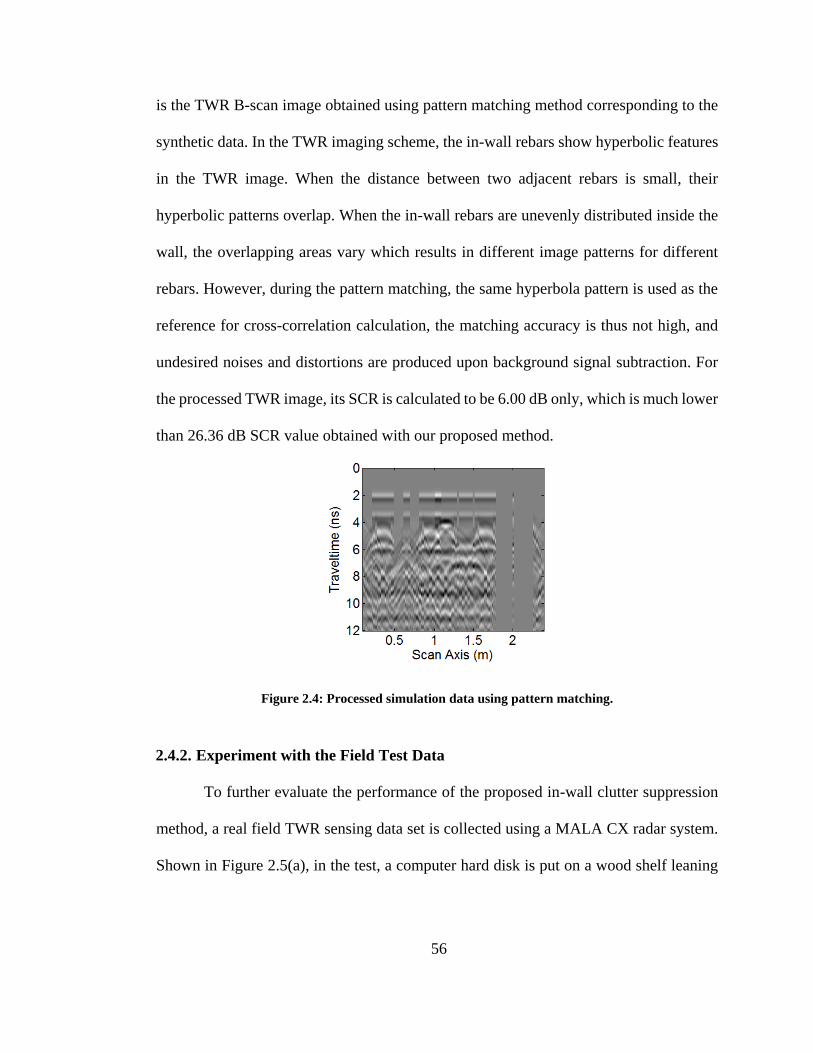
56

is the TWR B-scan image obtained using pattern matching method corresponding to the

synthetic data. In the TWR imaging scheme, the in-wall rebars show hyperbolic features

in the TWR image. When the distance between two adjacent rebars is small, their

hyperbolic patterns overlap. When the in-wall rebars are unevenly distributed inside the

wall, the overlapping areas vary which results in different image patterns for different

rebars. However, during the pattern matching, the same hyperbola pattern is used as the

reference for cross-correlation calculation, the matching accuracy is thus not high, and

undesired noises and distortions are produced upon background signal subtraction. For

the processed TWR image, its SCR is calculated to be 6.00 dB only, which is much lower

than 26.36 dB SCR value obtained with our proposed method.

Figure 2.4: Processed simulation data using pattern matching.

2.4.2. Experiment with the Field Test Data

To further evaluate the performance of the proposed in-wall clutter suppression

method, a real field TWR sensing data set is collected using a MALA CX radar system.

Shown in Figure 2.5(a), in the test, a computer hard disk is put on a wood shelf leaning

57

to the interior surface of a wall as the detection target. As depicted in Figure 2.5(b), the

TWR scan is performed on the other side of the wall.

(a) (b)

(c) (d)

Figure 2.5: Field test data: (a) A hard disk attached on the wall; (b) TWR scanning from the other

side of the wall; (c) MALA concrete imaging system; (d) Raw TWR image.

The radar system used in the test is MALA Concrete Imaging System coupled

with a MALA 2.3 GHz HF Antenna, which is shown in Figure 2.5(c). TWR data are

uniformly collected along the exterior wall surface at every 2.54 mm space. The raw

TWR image is plotted in Figure 2.5(d). The data matrix size is 312 × 884. In the raw

TWR image, the exterior wall reflection shows as a horizontal line at 1 ns, and the rebars

inside the wall are displayed as hyperbolic features locating between 1 ns and 3 ns. The

58

reflection signal from the hard disk at cross-section of 3 ns and 0.5 m is barely visible in

the raw TWR image for being masked by the strong background signal.

The pre-processed TWR is shown as Figure 2.6(a). In the pre-processed TWR

image, the wall surface reflection has been removed, however, the hard disk object

feature is still obscure comparing with the strong in-wall clutter, i.e. the repeated

hyperbolic features.

To solve the low-rank and sparse representation optimization problem to suppress

the correlated background data, tuning parameter 𝜆 = 1 √max (312, 884) ≈ 0.034⁄ is

substituted into Eq. (2.4). As shown in Figure 2.6(b), the target feature is enhanced upon

in-wall clutter suppression.

(a) (b)

Figure 2.6: Processed field test data: (a) Pre-processing – stationary background removal; (b) In-

wall clutter suppression.

To quantitatively analyze the in-wall clutter suppression result, SCRs of the TWR

images in the field test are calculated. For the pre-processed TWR image in Figure 2.6(a)

consisting of correlated background and object signal, the SCR is -18.20 dB. While for

59

the correlated background suppressed TWR image in Figure 2.6(b), the SCR becomes

17.75 dB. Apparently, the low-rank and sparse representation based in-wall clutter

removal method improves SCR by 35.95 dB comparing with the pre-processed TWR

image. The quantitative analysis results corroborate the effectiveness of the low-rank and

sparse representation based in-wall clutter suppression in TWR data processing.

Similar to the simulation data processing, the field test data in Figure 2.6(a) is

processed by the pattern matching method as well. The resulting image is plotted in

Figure 2.7. Due to the unevenly distribution of the in-wall clutter and the test

environmental noises, the in-wall clutter cannot be mitigated effectively utilizing the

pattern matching approach. The SCR of the processed TWR image is as low as -13.41

dB.

Figure 2.7: Processed field test data using pattern matching.

In sum, the proposed in-wall clutter suppression method based on low-rank and

sparse representation is more robust to the uneven distribution of the in-wall rebars or

pipes. Further, the proposed method does not produce fake scattering and undesired

image distortion comparing with the cross-correlation based pattern matching method.

60

2.5. Conclusions

In this letter, the correlated TWR image background suppression using low-rank

and sparse representation algorithm has been investigated, where the distribution of

targets under test is significantly sparser than that of the in-wall clutter. The proposed

method can automate the suppression of in-wall clutter, without the need of prior

knowledge about the target under test. Also, comparing with the conventional cross-

correlation based background subtraction methods, the proposed approach is insensitive

to the distribution of the correlated background matrix, which makes it effective for

practical use. Experiments with both the synthetic data and the field test data indicate

that the proposed in-wall clutter suppression technique can effectively improve the SCR

of the TWR image.

2.6. References

[1] M.G. Amin, “Through-the-Wall Radar Imaging,” CRC Press, 2011.

[2] A.S. Venkatachalam, X. Xu, D. Huston, and T. Xia, “Development of a New High

Speed Dual-Channel Impulse Ground Penetrating Radar,” IEEE Journal of

Selected Topics in Applied Earth Observations and Remote Sensing, vol. 7, no. 3,

pp. 753-760, Mar. 2014.

[3] Y. Zhang, G. Wang, and T. Xia, “Compressive orthogonal frequency division

multiplexing waveform based ground penerating radar,” 2015 IEEE Radar

Conference (RadarCon), pp. 684-689, 2015.

[4] A. Ahmed, Y. Zhang, D. Burns, D. Huston, and T. Xia, “Design of UWB Antenna

for Air-Coupled Impulse Ground-Penetrating Radar,” IEEE Geoscience and

Remote Sensing Letters, vol. 13, no. 1, pp. 92-96, 2016.

[5] F.H.C. Tivive, A. Bouzerdoum, and M.G. Amin, “A Subspace Projection


Transactions on Geoscience and Remote Sensing, vol. 53, no. 4, pp. 2108-2122,

Apr 2015.

[6] R. Solimene and A. Cuccaro, “Front Wall Clutter Rejection Methods in TWI,”

IEEE Geoscience and Remote Sensing Letters, vol. 11, no. 6, pp. 1158-1162, Jun

2014.

61

[7] Y.S. Yoon and M.G. Amin, “Spatial Filtering for Wall-Clutter Mitigation in

Through-the-Wall Radar Imaging,” IEEE Transactions on Geoscience and

Remote Sensing, vol. 47, no. 9, pp. 3192-3208, Sep 2009.

[8] Y. Zhang, A.S. Venkatachalam, D. Huston, and T. Xia, “Advanced signal


enhancement,” SPIE Smart Structures and Materials +Nondestructive Evaluation

and Health Monitoring, pp. 1-14, 2014.



Remote Sensing, vol. 44, no. 9, pp. 2393-2406, Sep 2006.

[10] Y. Zhang, A.S. Venkatachalam, T. Xia, Y. Xie, and G. Wang, “Data analysis

technique to leverage ground penetrating radar ballast inspection performance,”

2014 IEEE Radar Conference, Cincinnati, OH, pp. 463-468, May 2014.

[11] L. Li, A.E. Tan, K. Jhamb, and K. Rambabu, “Buried Object Characterization

Using Ultra-Wideband Ground Penetrating Radar,” IEEE Transactions on

Microwave Theory and Techniques, vol. 60, no. 8, pp. 2654 – 2664, Aug 2012.

[12] M. Richards, “Fundamentals of Radar Signal Processing,” McGraw-Hill

Education, 2005.

[13] Y. Zhang, P. Candra, G. Wang, and T. Xia, “2-D Entropy and Short-Time Fourier

Transform to Leverage GPR Data Analysis Efficiency,” IEEE Transactions on

Instrumentation and Measurement, vol. 64, no. 1, pp. 103-111, Jan 2015.

[14] Y. Zhang, A.S. Venkatachalam, and T. Xia, “Ground-penetrating radar railroad


detection efficiency,” Journal of Applied Remote Sensing, vol. 9, no. 1, pp. 1-19,

2015.

[15] J. Wright, Y. Peng, Y. Ma, A. Ganesh, and S. Rao, “Robust Principal Component

Analysis: Exact Recovery of Corrupted Low-Rank Matrices by Convex

Optimization,” Advances in Neural Information Processing Systems, pp. 2080-

2088, 2009.

[16] E.J. Candes, X. Li, Y. Ma, J. Wright, “Robust Principal Component Analysis?,”

Journal of the ACM, vol. 58, no. 3, article 11, pp. 1-37, May 2011.

[17] Y. Zhao and J. Yang, “Hyperspectral Image Denoising via Sparse Representation

and Low-Rank Constraint,” IEEE Transactions on Geoscience and Remote

Sensing, vol. 53, no. 1, pp. 296-308, Jan 2015.

[18] S. Jia, X. Zhang, and Q. Li, “Spectral-Spatial Hyperspectral Image Classificatin

Using 𝑙1/2 Regularized Low-Rank Representation and Sparse Representation-

Based Graph Cuts,” IEEE Journal of Selected Topics in Applied Earth

Observations and Remote Sensing, vol. 8, no. 6, pp. 2473-2484, Jun 2015.

[19] Y. Peng, A. Ganesh, J. Wright, W. Xu, and Y. Ma, “RASL: Robust Alignment by

Sparse and Low-Rank Decomposition for Linearly Correlated Images,” IEEE

Transactions on Pattern Analysis and Machine Intelligence, vol. 34, no. 11, pp.

2233-2246, Nov 2012.

62

[20] C. Dang and H. Radha, “RPCA-KFE: Key Frame Extraction for Video Using

Robust Principal Component Analysis,” IEEE Transactions on Image Processing,

vol. 24, no. 11, pp. 3742-3753, Nov 2015.

[21] E. Amaldi and V. Kann, “On the approximability of minimizaing nonzero

variables or unsatisfied relations in linear systems,” Theoretical Computer

Science, vol. 209, no. 1-2, pp. 237-260, Dec 1998.

[22] S.R. Becker, E.J. Candes, and M.C. Grant, “Templates for convex cone problems

with applications to sparse signal recovery,” Mathematical Programming

Computation, vol. 3, no. 3, pp. 165-218, Sep 2011.

[23] A. Giannopoulos, “Modeling ground penetrating radar by GprMax,” Construction

and Building Materials, vol. 19, no. 10, pp. 755-762, 2005.

63

CHAPTER 3: AIR COUPLED GROUND PENETRATING RADAR CLUTTER

MITIGATION FOR ROUGH SURFACE SENSING

Abstract

Ground penetrating radar (GPR) is a non-destructive evaluation technique

specifically effective for detecting buried objects. Due to the signal propagation loss, the

scattering from buried objects is much weaker than the clutter signal produced by the

ground surface. To extract the weak scattering from the subsurface object, removal of the

strong ground surface clutter is an issue of predominance. This chapter explores a low-

rank and sparse representation based signal decomposition technique to remove the

clutter produced by rough ground surface for air-coupled GPR, where the time instance

and the amplitude of surface clutter components in each A-Scan trace vary. The

performance of the proposed clutter removal method is evaluated through simulations

and laboratory experiments.

Keywords: ground penetrating radar, clutter removal, low-rank representation, sparse

representation, cross-correlation, non-destructive evaluation.

3.1. Introduction

GPR is a non-destructive evaluation technique specifically effective for detecting

buried objects [2]-[5]. Based on antenna configurations, GPR system can be typically

classified as ground-coupled GPR and air-coupled GPR. Comparing with the ground-

coupled GPR system, the air-coupled GPR sensing provides the benefit of high survey

speed due to the large standoff distance between the antennas and the ground surface.

Whereas the large standoff distance leads to significant propagation losses [1], the

64

reflection signal amplitude from the subsurface object is greatly reduced. In order to

extract the weak scattering from the subsurface object, removal of the strong ground

surface clutter is an issue of predominance for air-coupled GPR signal processing.

Many clutter removal methods have been investigated in the literature, which

generally deal with relatively flat ground surfaces. These methods include average

subtraction [7], spatial filtering [8]-[9], etc. Assuming the clutter in each A-Scan shows

high similarity, the average subtraction method calculates the average of different A-

Scan traces as the background signal, which is then subtracted from each A-Scan to

remove the clutter while enhance the target scattering signal. Spatial filtering method

utilizes the same assumption to filter out the clutter data corresponding to the ground

surface reflection. Considering the reflection signal from the buried object with limited

spatial extent varies in different A-scan traces, a spatial filter is thus applied along the

antenna moving direction to mitigate the spatial zero-frequency and low-frequency

components corresponding to clutter. When the ground surface conditions are

complicatedly rough, the effectiveness of average subtraction and spatial filtering clutter

removal algorithms is degraded. Some other clutter removal methods can deal with rough

ground surfaces, such as subspace projection approach [5], principal component analysis

(PCA) [11], independent component analysis (ICA) [12], time gating [13], etc. The

subspace projection approach is based on the reflection energy difference between the

ground surface and the buried object. Singular value decomposition (SVD) is performed

on the data matrix to identify and remove the ground surface electromagnetic signature.

Unfortunately, it is infeasible to determine an appropriate threshold value for the

65

subspace projection when no prior-knowledge about the underground structure is

available. PCA and ICA methods also decompose the GPR data into subspace

components, and then select a subset of components containing buried object

information. However, the components selection process is performed with intensive

human interventions. In the time gating method, a windowing function is defined to null

the signal segments over the time intervals where different signal traces exhibit a high

similarity, which facilitates clutter signal removal. However, the accuracy of time gating

method is low when the target is shallowly buried where the ground clutter and target

scattering overlap.

To tackle such problems, in this chapter, a low-rank and sparse representation

based signal decomposition technique is explored to remove the clutter produced by

rough ground surface reflection. The low-rank and sparse representation method has been

proved to be effective in modeling the ground clutter data in GPR B-Scan images [14]-

[18]. Those methods assume the clutter components in A-Scan signals are at the same

depth level. In other words, they only deal with relatively flat ground surface. For rough

or non-flat ground surface, the surface clutter components in different A-Scan traces are

not aligned on the depth axis. To compensate for the misalignments so as to facilitate the

clutter removal, in this chapter, the A-Scan traces in a GPR data matrix are aligned using

cross-correlation method. The low-rank and sparse representation technique is then

developed to decompose the aligned GPR data matrix into two sub-matrices: a low-rank

matrix whose column data record the ground clutter in A-Scan traces, and a sparse matrix

that features the subsurface object. This chapter is an extension of the work presented in

66

a previous SPIE conference [19], where the preliminary study was performed. In this

chapter, a Renyi entropy based analysis is developed to fine tune the clutter removal.

More quantitative analysis on the methodology and experimental results are also

conducted. Simulations and actual lab measurements are performed to evaluate the

effectiveness of the proposed method.

The rest sections of the chapter are organized as followings. Sec. 3.2 models the

clutter on rough ground surface as a low-rank and sparse representation problem, and

Sec. 3.3 describes the proposed clutter removal methodology. In Sec. 3.4, the

effectiveness of the proposed method is evaluated using finite-difference time-domain

(FDTD) simulation and real lab experiments. Sec. 3.5 summarizes the concluding

remarks.

3.2. GPR B-Scan Image Model

In GPR survey, the signal collected at the 𝑛th observation position can be modeled

as

𝑑𝑛(𝑡) = 𝑙𝑛(𝑡) + 𝑠𝑛(𝑡) (3.1)

where 𝑑𝑛(𝑡) is the received A-Scan signal, 𝑙𝑛(𝑡) is the clutter due to ground surface

reflection, and 𝑠𝑛(𝑡) is the reflection signal from the buried target.

For GPR imaging, 𝑑𝑛(𝑡), 𝑙𝑛(𝑡) and 𝑠𝑛(𝑡) are recorded as 𝑀 × 1 vectors 𝒅𝒏, 𝒍𝒏,

and 𝒔𝒏 respectively. 𝑀 is the number of samples collected at each scan position.

Assembling the data of all 𝑁 scan positions leads to the following 𝑀 × 𝑁 data matrices:

𝑫 = [𝒅𝟏, 𝒅𝟐, 𝒅𝟑, … , 𝒅𝑵] (3.2)

𝑳 = [𝒍𝟏, 𝒍𝟐, 𝒍𝟑, … , 𝒍𝑵] (3.3)

67

𝑺 = [𝒔𝟏, 𝒔𝟐, 𝒔𝟑, … , 𝒔𝑵] (3.4)

In Eq. (3.2) – Eq. (3.4), 𝑫 ∈ ℝ𝑀×𝑁 is the observed GPR B-Scan image data matrix, 𝑳 ∈

ℝ𝑀×𝑁 is the data matrix featuring the ground clutter, and 𝑺 ∈ ℝ𝑀×𝑁 is the data matrix

featuring the buried target, where 𝑀 represents the number of data points in each A-Scan

trace, and 𝑁 represents the total number of A-Scan traces. According to Eq. (3.1), it has

𝑫 = 𝑳 + 𝑺 (3.5)

For rough or non-flat ground surface, the surface clutter components

𝒍𝟏, 𝒍𝟐, 𝒍𝟑, … , 𝒍𝑵 in different A-Scan traces 𝒅𝟏, 𝒅𝟐, 𝒅𝟑, … , 𝒅𝑵 are not aligned on the depth

axis. To compensate for these misalignments so as to facilitate clutter removal, the cross-

correlation technique is applied.

The first A-Scan signal 𝑑1(𝑡) is selected as the reference trace, and the cross-

correlation between 𝑑1(𝑡) and 𝑑𝑛(𝑡) is calculated to specify the time offset between the

ground reflection of 𝑑𝑛(𝑡) and 𝑑1(𝑡) on the depth axis [20]. Assuming the optimal time

offset computed from the cross-correlation analysis is ∆𝑡𝑛, the alignment operation on

the 𝑛th A-Scan trace can be defined as

𝑑𝑛′ (𝑡) = 𝑑𝑛(𝑡 − ∆𝑡𝑛) (3.6)

Substituting Eq. (3.6) into the signal model in Eq. (3.1), the resulting signal model upon

alignment can be expressed as

𝑑𝑛′ (𝑡) = 𝑙𝑛

′ (𝑡) + 𝑠𝑛′ (𝑡) (3.7)

In this transformed model, 𝑙𝑛′ (𝑡) is the clutter signal upon alignment adjustment, and

𝑠𝑛′ (𝑡) is the target scattering upon alignment adjustment. Since the alignment adjustment

is a linear operation, the following relation between 𝑠𝑛(𝑡) and 𝑠𝑛′ (𝑡) exists:

68

𝑠𝑛′ (𝑡) = 𝑠𝑛(𝑡 − ∆𝑡𝑛) (3.8)

In this chapter, the low-rank and sparse representation technique is utilized to separate

the correlated background clutter 𝑙𝑛′ (𝑡) and the target signature 𝑠𝑛

′ (𝑡).

Upon the alignment adjustment, the corresponding GPR B-Scan image model in

Eq. (3.5) can be expressed as

𝑫′ = 𝑳′ + 𝑺′ (3.9)

Since each column of 𝑳′ is the ground clutter upon alignment adjustment, the rank of

matrix 𝑳′ is low. For the buried small and spatially sparse targets, it results in 𝑺′ being a

sparse matrix.

3.3. Low-Rank and Sparse Decomposition Based Clutter Removal

The low-rank and sparse representation [21] interprets the data matrix 𝑫′ as a

superposition of a low-rank matrix 𝑳′̂ ∈ ℝ𝑀×𝑁 and a sparse matrix 𝑺′̂ ∈ ℝ𝑀×𝑁, where 𝑳′̂

represents the correlated clutter, while 𝑺′̂ models the target features on top of the

correlated clutter. The mathematical expression is 𝑫′ = 𝑳′̂ + 𝑺′̂.

Decomposing the data matrix 𝑫′ into 𝑳′̂ and 𝑺′̂ is an optimization problem.

Through Lagrangian reformulation, it can be expressed as:

min𝐿,𝑆

𝑟𝑎𝑛𝑘(𝑳′̂) + 𝜆‖𝑺′̂‖0

𝑠. 𝑡. 𝑫′ = 𝑳′̂ + 𝑺′̂ (3.10)

Unfortunately, Eq. (3.10) is a highly nonconvex optimization problem subsuming both

the low rank matrix completion and the 𝑙0-minimization, which are both NP-hard. By

replacing 𝑙0-norm with 𝑙1-norm, and the rank of 𝐿 with the nuclear norm ‖𝐿‖∗ =

∑ 𝜎𝑖(𝐿)𝑖 , a tractable optimization problem can be obtained [21]:

min𝐿,𝑆

‖𝑳′̂‖∗

+ 𝜆‖𝑺′̂‖1

𝑠. 𝑡. 𝑫′ = 𝑳′̂ + 𝑺′̂ (3.11)

69

where ‖𝑳′̂‖∗ is the nuclear norm or sum of singular values of matrix 𝑳′̂, ‖𝑺′̂‖

1 is the 𝑙1-

norm or sum of absolute values of the entries of 𝑺′̂, and 𝜆 is a tuning parameter that

balances the contribution of the 𝑙1-norm term relative to the nuclear norm term. Choice

of 𝜆 = 1 √max (𝑀, 𝑁)⁄ is universal for solving the optimization problem in Eq. (3.11).

According to Ref. [22], in the general rectangular case, where 𝑀 ≥ 𝑁, if

𝑟𝑎𝑛𝑘(𝑳′) ≤ 𝜌𝑟𝑁

(log 𝑀)2 (3.12)

and

‖𝑺′‖0 ≤ 0.1 ∗ 𝑀𝑁 (3.13)

matrix 𝑳′ and 𝑺′ can be uniquely reconstructed by solving Eq. (3.11), which means 𝑳′ =

𝑳′̂ and 𝑺′ = 𝑺′̂. In Eq. (3.12), 𝜌𝑟 is a positive constant coefficient, which means the rank

of 𝑳′ is of the order of 𝑁

(log 𝑀)2.

Upon the decomposition, the matrix 𝑳′ contains the clutter and some subsurface

background information. The subsurface background information are of interest for GPR

applications, such as pavement subsurface characterization [2],[23], layer thickness

measurement [24]-[25], subsurface dielectric property analysis [26], soil moisture

estimation [27], etc. Since the proposed clutter removal method only aims to eliminate

the clutter produced by the ground surface, the subsurface background information can

be preserved and extracted in conjunction with the sparse target matrix 𝑺′.

A Renyi entropy-based time gating method [5],[13],[28] is applied to extract the

ground surface clutter components in the matrix 𝑳′. In the low-rank matrix 𝑳′, the signal

envelope along the range direction is calculated with the Hilbert Transform and the

70

produced envelope matrix is denoted as 𝐿𝑒. The data in 𝐿𝑒 are normalized alone the radar

cross-range direction (or the GPR scanning direction) as:

�̃�𝑒(𝑚, 𝑛) =|𝐿𝑒(𝑚,𝑛)|2

∑ |𝐿𝑒(𝑚,𝑛)|2𝑁𝑛=1

(3.14)

Upon the normalization, the Renyi’s entropy [29] along the radar cross-range

direction is calculated as:

𝐸𝛼(𝑚) =1

1−𝛼log𝑒(∑ �̃�𝑒(𝑚, 𝑛)𝛼𝑁

𝑛=1 ) (3.15)

where 𝐸𝛼(𝑚) is the entropy quantification and 𝛼 is the entropy order. According to the

experiments and analysis in Ref. [5], 𝛼 = 3 is the optimal configuration for GPR

applications. As the ground surface clutter signal components have similar shapes, they

result in large values of 𝐸𝛼(𝑚) [13],[28]. Therefore, a windowing along the range

direction that marks the ground surface clutter signals region can be determined as [28]:

𝑊(𝑚, 𝑛) = {0, 𝑖𝑓 𝐸𝛼(𝑚) ≥ 𝛽 log𝑒 𝑁1, 𝑒𝑙𝑠𝑒𝑤ℎ𝑒𝑟𝑒

(3.16)

𝛽 is the tuning parameter that accounts for the measurement noise in the GPR signal,

which is optimized at 𝛽 = 0.97 for radar applications according to the analysis in Ref.

[28]. Denoting the window function 𝑊(𝑚) ranges between time instance 0 and 𝑡𝑑, based

on the entropy analysis, the signals of time instances within 0 and 𝑡𝑑 are considered as

the ground surface clutter signals, whose values are set as zero, and the resulting matrix

is recorded as 𝑳𝒔𝒖𝒃′ :

𝑳𝒔𝒖𝒃′ (𝑚) = 𝑳′(𝑚, 𝑛)𝑊(𝑚, 𝑛) (3.17)

In this way, the nulling is only performed on matrix 𝑳′ featuring the clutter signal,

while the matrix 𝑺′ featuring the buried object scattering is preserved. Comparing to

71

traditional time gating [13] method that nulls the whole data matrix 𝑫′, the proposed

method does not smear the scattering data of the buried object when the object is close

to the ground surface.

The overall subsurface data matrix can be expressed as:

𝑺𝒑𝒓𝒐𝒄′ = 𝑺′ + 𝑳𝒔𝒖𝒃

′ (3.18)

Once matrix 𝑺𝒑𝒓𝒐𝒄′ is obtained, the matrix of the original object matrix𝑺 can be

reconstructed by reversing the alignment adjustment process using the time offset value

obtained with Eq. (3.8).

Figure 3.1: Ground clutter removal process

Finally, the clutter removal procedures for rough ground surface are summarized

below:

1. Alignment: Align each A-Scan trace in the B-Scan image 𝑫 using cross-correlation

criterion to obtain a processed B-Scan image 𝑫′.

72

2. Decompose the processed GPR B-Scan data matrix 𝑫′ ∈ ℝ𝑀×𝑁 into a low-rank

matrix 𝑳′ ∈ ℝ𝑀×𝑁 and a sparse matrix 𝑺′ ∈ ℝ𝑀×𝑁 by solving Eq. (3.11) with tuning

parameter 𝜆 = 1 √max (𝑀, 𝑁)⁄ .

3. Calculate the envelope of the signal in matrix 𝑳′ along the range direction. Determine

and null the clutter region whose depth is above 𝑡𝑑 based on Renyi entropy analysis

to obtain matrix 𝑳𝒔𝒖𝒃′ as illustrated in Figure 3.1.

4. Compensate the subsurface medium information in matrix 𝑳𝒔𝒖𝒃′ to the sparse matrix

𝑺′ following Eq. (3.18).

5. Revere time alignment adjustment of the sparse matrix 𝑺𝒑𝒓𝒐𝒄′ to reproduce the buried

target features in the B-Scan image.

3.4. Experimental results

To evaluate the proposed clutter removal method for rough ground surface

inspection, experiments are conducted with two sets of test data. The first set of data is

synthesized with the GPR simulation tool GprMax [30] while the second one is the

laboratory experimental data collected using a step-frequency continuous wave radar

(SFCW) system. The optimization problem in Eq. (3.11) is solved utilizing the

mathematical toolbox TFOCS [31].

3.4.1. Simulation Data 1: Oblique Ground Surface

In this section, two sets of simulation data are created using GprMax program. In

the first simulation setup: the ground is modeled as a homogeneous layer with oblique

surface whose dielectric constant is 6.0. The slope of the oblique surface is 5°. The buried

target is modeled as a cylinder of 1.25 cm radius with 4.0 dielectric constant. The test

73

geometry detail for this test case is depicted in Figure 3.2(a). The GprMax program is

developed with FDTD technique. In our simulation, the GPR waveform is generated as

a Ricker waveform (i.e. negative normalized second derivative of a Gaussian pulse) with

its center frequency being 900 MHz. GPR A-Scan traces are collected uniformly from

left to right along the horizontal direction every 2 cm distance in air-coupled mode. The

standoff distance between the transceiver antennas and the ground surface is 30 cm. The

separation distance between the transmitter antenna and the receiver antenna is 2.5 cm.

The size of the data matrix is 962 × 46.

The raw GPR B-scan image is plotted in Figure 3.2(b), in which the strongest

reflection between 0.5 ns and 1.3 ns time interval is the clutter due to the ground surface

reflection, and the weak hyperbolic curve at 2.5 ns is the reflection signal from the buried

target. Correspondingly, some A-Scan traces selected at different scan positions from the

B-Scan image are plotted in Figure 3.3. As shown, the strongest peak in each A-Scan

trace is the ground surface clutter, whose time index shifts among different traces. For

these misaligned ground surface clutter signals in A-Scan traces, they cannot be

eliminated using traditional clutter removal method, i.e. average subtraction [7]. Figure

3.2(c) shows the average subtraction method fails to improve the target feature in the B-

Scan image.

74

(a) (b) (c)

Figure 3.2: Synthetized oblique ground surface: (a) Geometry data; (b) Raw B-scan image; (c)

Average subtraction from raw B-Scan.

Figure 3.3: Synthesized oblique ground surface: A-Scan trace at various locations along scan axis.

By applying the alignment adjustment, the resulting GPR B-Scan image is plotted

in Figure 3.4(a). Figure 3.4(b) and (c) depict the processed B-Scan images upon average

subtraction and the proposed clutter removal to the aligned B-Scan image respectively.

As shown in Figure 3.4(b), the average subtraction can enhance the target features,

however, the residual clutter still exists around time instance 1 ns. Since the alignment is

performed on the digitized data, the finest time resolution for adjustment equals the

sampling time interval of the data acquisition unit (or analog-to-digital converter), which

is ∆𝑡 = 6 ps in this simulation test case. As the radar clutter is produced from the ground

75

surface reflection and the radar wave propagation velocity is 𝑐 = 3 × 108 m/s in the air,

the achievable depth resolution for alignment is ∆𝑑 = (∆𝑡/2) ∗ 𝑐 = 0.9 mm. In other

words, the alignment algorithm cannot fix the depth displacement smaller than 0.9 mm.

(a) (b) (c)

Figure 3.4: Synthetic oblique ground surface: (a) Aligned B-Scan; (b) Clutter removal using

average subtraction; (c) Clutter removal using proposed method.

With our proposed clutter removal method, the smaller-than-resolution

displacement can be processed as a low rank component within the data matrix, which

can be separated and removed from the reflection signals of the underground target.

Figure 3.4(c) illustrates the B-scan image upon clutter removal. As can be observed, the

hyperbolic pattern corresponding to the burying cylinder is much more pronounced.

3.4.2. Simulation Data 2: Rough Ground Surface

In the second simulation setup, the ground is modeled as a homogeneous layer

with wiggly surface. The heights of the wiggles vary randomly between 3 cm and 7 cm.

The layer’s dielectric constant is 6.0. The buried target is a reinforce bar of 2.5 cm radius

and its burying depth is 10 cm. The test geometry for this test case is depicted in Figure

76

3.5(a). In the FDTD simulation, the same GPR waveform and scan along the horizontal

direction as Simulation 1 are utilized. The data matrix dimension is 972 × 46.

The raw GPR B-scan image obtained is plotted in Figure 3.5(b), in which the

strongest reflections between 0.5 ns and 1.2 ns time interval are the ground surface

clutter, and the weak hyperbolic curve at 2 ns features the reflection signal from the

buried rebar. Selected A-Scan traces at different scan locations are plotted in Figure 3.6.

The foremost strong pulse in each A-Scan trace is the ground surface clutter with varying

amplitude and position. Without alignment adjustment, it is infeasible to suppress such

ground surface clutter. For instance, the clutter removal result with the traditional average

subtraction [7] method is depicted in Figure 3.5(c). As can be observed, the hyperbolic

feature is enhanced, however the clutter components remain between 1 ns and 2 ns time

interval.

(a) (b) (c)

Figure 3.5: Synthetic rough ground surface: (a) Geometry data; (b) Raw B-scan image; (c)

Average subtraction from raw B-Scan.

77

Figure 3.6: Synthesized rough ground surface: A-Scan trace at various locations along scan axis.

After the alignment adjustment, the resulting GPR B-Scan image is plotted in

Figure 3.7(a). Figure 3.7(b) and (c) illustrate the processed B-Scan images upon average

subtraction and proposed clutter removal. As shown in Figure 3.7(b), the average

subtraction improves the target features, however is not able to remove the clutter. After

applying the proposed clutter removal method, as shown in Figure 3.7(c), the hyperbolic

pattern is enhanced and the clutter is largely eliminated.

(a) (b) (c)

Figure 3.7: Synthetic rough ground surface: (a) Aligned B-Scan; (b) Clutter removal using average

subtraction; (c) Clutter removal using the proposed method.

78

3.4.3. Experiment with Lab Test Data

The proposed clutter removal method is also evaluated using real experimental

data collected via a step-frequency continuous wave GPR system. In this GPR system,

the transmitter and data acquisition unit employed is Keysight N9917A FieldFox

Microwave Analyzer whose operating frequency spans from 30 kHz to 18 GHz. The

transceiver antennas are a pair of customized horn antennas [32] whose bandwidth spans

from 600 MHz to 6 GHz. The test setup is depicted in Figure 3.8(a). A metal plate is

buried in a sandbox as the target under test. The metal plate is 0.64 cm thick, 30.5 cm

long, 20.3 cm wide and is buried 8 cm deep. Water is sprayed on sand surface to emulate

moisture in real field GPR test scenario. The transmitter and receiver antennas are set 71

cm above the sand surface. The angle of incidence and angle of reflection are both 45

degree. The scan is performed along the longitudinal direction. The dimension of GPR

data matrix is 400 × 152.

The raw GPR B-scan image is plotted in Figure 3.8(b), in which the strongest

reflection at 0.45 ns is the sand surface clutter, and the hyperbolic feature at 1 ns is the

reflection from the buried plate. Figure 3.8(c) shows the clutter removal result using

traditional average subtraction [7] method, which even makes the target feature worse in

the B-Scan image.

79

(a) (b) (c)

Figure 3.8: Lab sandbox test: (a) Geometry data; (b) Raw B-scan image; (c) Average subtraction

from raw B-Scan.

Upon the alignment, the resulting GPR B-Scan image is plotted in Figure 3.9(a).

Figure 3.9(b) shows the processed B-Scan image with average subtraction, where the

sand surface clutter is removed, whereas additional clutter is induced around 1 ns depth

as the dark horizontal line. Figure 3.9(c) shows the processed B-Scan using the proposed

clutter removal method. Comparing to the average subtraction method, the proposed

method can suppress the sand surface clutter while not produce any fake scattering

features.

(a) (b) (c)

Figure 3.9: Lab sandbox test: (a) Aligned B-Scan; (b) Clutter removal using average subtraction;

(c) Clutter removal using the proposed method.

80

3.4.4. Quantitative Analysis on the Processed Data

To quantitatively evaluate the clutter removal method performance, signal-to-

clutter ratio (SCR) is used as a metric for characterizing the power ratio between the

backscattering signal from the buried object under test and the clutter in each test case.

The SCR of raw B-Scan images, the processed B-Scan image using average subtraction

and the processed B-Scan image using the proposed clutter removal are calculated for all

three test cases. The SCR calculation results are summarized in Table 3.1. The quantitative

analysis results indicate that the proposed clutter removal method can dramatically enhance

the buried object features in GPR B-Scan image, and outperforms the traditional average

subtraction method.

Table 3.1: SCR of each B-Scan Image.

Test Case

SCR of

Raw B-

Scan (dB)

SCR of Processed B-Scan

using Average Subtraction

(dB)

SCR of Processed B-

Scan using Proposed

Method (dB)

Simulation

Data 1 -22.86 6.23 14.86

Simulation

Data 2 -3.75 8.75 14.58

Lab

Experiment

Data

2.60 7.85 23.08

81

3.5. Conclusions

In this chapter, a low-rank and sparse representation based clutter removal

technique has been investigated. In the observed data matrix upon alignment, the clutter

component produced by the rough ground surface are modeled as a low-rank matrix, and

the scattering from the buried objects are modeled as a sparse matrix. The convex

optimization is applied to decompose the observed data matrix into the low-rank matrix

and the sparse matrix, to extract the weak scattering features from the strong clutter

signal. Since the proposed method characterizes the rank of the clutter components in the

data matrix instead of merely the amplitude of the clutter signal, the proposed clutter

removal method can effectively suppress the clutter generated by rough ground surface

in GPR field inspection. Experiments with the simulation data and lab testing data are

conducted for performance validation. In the first simulation test, the proposed clutter

removal method improves SCR by 37.72 dB. In the second simulation test, the proposed

method improves SCR by 18.33 dB. For the lab experimental data, 20.48 dB SCR

improvement is achieved.

3.6. References

[1] A. S. Venkatachalam, X. Xu, D. Huston, and T. Xia, “Development of a New High


Selected Topics in Applied Earth Observations and Remote Sensing 7(3), 753-760

(2014).

[2] H. Liu, R. Birken, and M. L. Wang, “Automatic pavement layer identification with

multichannel ground penetrating radar at traffic speed,” Journal of Applied

Remote Sensing 10(4), 046023 (2016).

[3] Y. Zhang, D. Burns, D. Huston, and T. Xia, “Sand moisture assessment using

instantaneous phase information in ground penetrating radar data,” Proc. SPIE

9437, 943726 (2015).

82

[4] H. Zhang, S. Ouyang, G. Wang, S. Wu, and F. Zhang, “Matched filtering

algorithm based on phase-shifting pursuit for ground-penetrating radar signal

enhancement,” Journal of Applied Remote Sensing 8(1), 083593 (2014).

[5] Y. Zhang, P. Candra, G. Wang, and T. Xia, “2-D entropy and short-time Fourier

transform to leverage GPR data analysis efficiency,” IEEE Transactions on

Instrumentation and Measurement 64(1), 103-111 (2015).

[6] H. M. Jol, Ground Penetrating Radar Theory and Applications, Elsevier (2008).

[7] G. R. Olhoeft, “Maximizing the information return from ground penetrating

radar,” Journal of Applied Geophysics 43(2), 175-187 (2000).



Remote Sensing 44(9), 2393-2406 (2006).

[9] Y. Zhang, A. S. Venkatachalam, D. Huston, and T. Xia, “Advanced signal


enhancement,” Proc. SPIE 9063, 906318 (2014).

[10] F. H. C. Tivive, A. Bouzerdoum, and M. G. Amin, “A Subspace Projection


Transactions on Geoscience and Remote Sensing 53(4), 2108-2122 (2015).

[11] P. K. Verma, A. N. Gaikwad, D. Singh, and M. J. Nigam, “Analysis of clutter

reduction techniques for through wall imaging in UWB range,” Progress In

Electromagnetics Research B 17, 29-48 (2009).

[12] B. Karlsen, H. B. Sorensen, J. Larsen, and K. B. Jakobsen, “Independent

component analysis for clutter reduction in ground penetrating radar data,” Proc.

SPIE 4742, 378-389 (2002) [doi: 10.1117/12.479110].

[13] R. Solimene, and A. Cuccaro, “Front Wall Clutter Rejection Methods in TWI,”

IEEE Geoscience and Remote Sensing Letters 11(6), 1158-1162 (2014).

[14] Y. Zhang, and T. Xia, “In-Wall Clutter Suppression based on Low-Rank and

Sparse Representation for Through-the-Wall Radar,” IEEE Geoscience and

Remote Sensing Letters 13(5), 671-675 (2016).

[15] Y. Zhang, and T. Xia, “Extracting sparse crack features from correlated

background in ground penetrating radar concrete imaging using robust principal

component analysis technique,” Proc. SPIE 9804, 980402 (2016).

[16] D. Kalika, M. T. Knox, L. M. Collins, P. A. Torrione, and D. Morton, “Leveraging

robust principal component analysis to detect buried explosive threats in handheld

ground-penetrating radar data,” Proc. SPIE 9454, 94541D (2015).

[17] A. Bouzerdoum, F. H. C. Tivive, and C. Abeynayake, “Target detection in GPR

data using joint low-rank and sparsity constraints,” Proc. SPIE 9857, 98570A

(2016).

[18] M. P. Masarik, J. Burns, B. T. Thelen, J. Kelly, T. C. Havens, “GPR anomaly

detection with robust principal component analysis,” Proc. SPIE 9454, 945414

(2015).

83

[19] Y. Zhang, D. Burns, D. Orfeo, D. R. Huston, and T. Xia, “Rough ground surface

clutter removal in air-coupled ground penetrating rdar data using low-rank and

sparse representation,” SPIE Smart Structures/NDE 2017, (2017).

[20] Y. Zhang, A. S. Venkatachalam, and T. Xia, “Ground-penetrating radar railroad


detection efficiency,” Journal of Applied Remote Sensing 9(1), 095058 (2015).

[21] E. J. Candes, X. Li, Y. Ma, and J. Wright, “Robust Principal Component

Analysis?,” Journal of the ACM 58(3), 1-37 (2011).

[22] J. Wright, Y. Peng, Y. Ma, A. Ganesh, and S. Rao, “Robust Principal Component

Analysis: Exact Recovery of Corrupted Low-Rank Matrices by Convex

Optimization,” Advances in Neural Information Processing Systems 22, 2080-

2088 (2009).

[23] A. Loizos, and C. Plati, “Accuracy of Ground Penetrating Radar Horn-Antenna

Technique for Sensing Pavement Subsurface,” IEEE Sensors Journal 7(5), 842-

850 (2007).

[24] I. Al-Qadi, S. Lahouar, K. Jiang, K. McGhee, D. Mokarem, “Accuracy of Ground-

Penetrating Radar for Estimating Rigid and Flexible Pavement Layer

Thicknesses,” Transportation Research Record: Journal of the Transportation

Research Board 1940, 69-78 (2005).

[25] D. A. Willett, K. C. Mahboub, and B. Rister, “Accuracy of Ground-Penetrating

Radar for Pavement-Layer Thickness Analysis,” Journal of Transportation

Engineering 132(1), 96-103 (2006).

[26] S. Lambot, E. C. Slob, I. V. D. Bosch, B. Stockbroeckx, and M. Vanclooster,

“Modeling of ground-penetrating radar for accurate characterization of subsurface

electric properties,” IEEE Transactions on Geoscience and Remote Sensing

42(11), 2555-2568 (2004).

[27] I. A. Lunt, S. S. Hubbard, and Y. Rubin, “Soil moisture content estimation using

ground-penetrating radar reflection data,” Journal of Hydrology 307(1-4), 254-

269 (2005).

[28] R. Solimene, and A. D'Alterio, “Entropy-based clutter rejection for intrawall

diagnostics,” International Journal of Geophysics, 2012, (2012).

[29] R. G. Baraniuk, P. Flandrin, A. J. E. M. Janssen, and O. Michel, “Measuring time-

frequency information content using the Renyi entropies,” IEEE Transactions on

Information Theory 47(4), 1391–1409 (2001).

[30] A. Giannopoulos, “Modeling ground penetrating radar by GprMax,” Construction

and Building Materials 19(10), 755-762 (2005).

[31] S. R. Becker, E. J. Candes, and M. C. Grant, “Templates for convex cone problems

with applications to sparse signal recovery,” Mathematical Programming

Computation 3(3), 165-218 (2011) [doi: 10.1007/s12532-011-0029-5].

[32] A. Ahmed, Y. Zhang, D. Burns, D. Huston, and T. Xia, “Design of UWB Antenna

for Air-Coupled Impulse Ground-Penetrating Radar,” IEEE Geoscience and

Remote Sensing Letters 13(1), 92-96 (2015).

84

CHAPTER 4: 2-D ENTROPY AND SHORT-TIME FOURIER TRANSFORM

TO LEVERAGE GPR DATA ANALYSIS EFFICIENCY

Abstract

Accurate detection of singular region using Ground Penetrating Radar (GPR) is

very useful in assessing roadway pavement, bridge deck concrete structure and railroad

ballast conditions. To locate object within the large radargram, it involves extensive

computational resources and time, especially when the data of interests only possess a

small portion of the whole big data set. Therefore an efficient GPR signal processing

technique is highly demanded. This chapter proposes the utilization of two-dimensional

(2D) entropy analysis to narrow down the data scope to the interested regions, which can

considerably reduce computational cost for more sophisticated post data processing.

Joint time-frequency analysis using Short Time Fourier Transform (STFT) is then

performed for singular region location detection and refinement. The proposed

methodology is tested with different laboratory setups. The analysis results show good

agreements with physical configurations.

Keywords: Radar; Signal processing; Entropy; Radar detection; Nondestructive testing.

4.1. Introduction

Impulse Ground penetrating radar (GPR) has been proven to be an effective tool

in inspecting transportation infrastructures, including bridge deck [1]-[4], highway

pavement and railroad ballast [5], [6], for its ability to extract subsurface information in

a nondestructive manner. For GPR, one important and challenging design factor is signal

processing, whose objective is to effectively analyze and extract meaningful information,

85

and accurately interpret the measurement results. In this chapter, a new signal processing

approach is developed to leverage GPR data analysis efficiency with a specific focus on

singular region detection.

For transportation infrastructure survey, detecting sporadically located singular

regions, such as embedded rebars is one of the basic functions for GPR subsurface

structure examination. Many data processing techniques have been developed for rebar

detection. In Ref. [1], an energy function is used to model and detect rebar hyperbolic

signature pattern and iterative hyperbola curve fitting is applied. Although this method

is effective, the long computation time limits its applicability only to small volume radar

data set. Moreover, the curve fitting method is only applicable when the characteristic

pattern is pre-known, and is not valid for detecting a singular region of an arbitrary shape.

In Ref. [2], an approximate linear scattering model is developed utilizing the sparse

nature of scatters to reconstruct the reflection signal. The reconstruction model is a

double integral, and a minimization algorithm is implemented by loops of matrix

multiplication. This method can precisely locate rebar. However the processing

procedures are relatively complicate. In Ref. [3]-[6], rebar GPR B-scan image signature

curves are characterized through a series of image processing algorithms such as image

segmentation, arc detection and curve fitting. The same processing steps are performed

throughout the entire scanning data even though the interested rebar data only populate

a small portion of the dataset. While such approaches are meticulous, they are both costly

and time consuming. Therefore to develop a method to automate the detection of

86

sporadically distributed singular regions of arbitrary shapes for facilitating sophisticated

post-processing is highly desired.

In this chapter, two-dimensional (2D) entropy analysis algorithm is developed to

effectively reduce the data scope to the singular regions within the large background. In

information theory, entropy is a measure of the uncertainty associated with a random

variable [7]. It has been applied in several application fields such as biomedical

engineering [8], [9], speech [10], information data mining [11], front wall clutter

rejection [12] and color image enhancement [13]. However to date, there has been no

literature utilizing entropy analysis on GPR image for detecting the sporadically

distributed features. In this chapter, 2D entropy processing algorithm is developed for

object extraction from the stationary background. As a result, the distinctive areas of

interests can be rapidly identified, and the size of the data for post-processing can be

significantly reduced. For GPR data post-processing, one important analytical approach

is spectrum characterization with Fourier transform. However the main limitation is that

the signal time information is lost in transforming to the frequency domain. For a

stationary signal analysis, where the processed signals do not change with time, this

limitation is not an issue. While in GPR scans, the premise of stationary signal does not

hold. During GPR operation, the scanning antennas move continuously, thus the

subsurface features under inspection change dynamically, which lead to non-stationary

reflection signals being collected. In order to obtain time and spectrum information from

GPR signals, the joint time-frequency (JTF) signal decomposition is employed. JTF

signal decomposition is a special form of spectral analysis that aims at precise tracking

87

frequencies of non-stationary time-varying signals. However the application of JTF

analysis for GPR signal processing is very limited. A major barrier is the computational

cost associated with the large data size, typically over tens of Giga-bytes (GBs). Directly

performing complicate JTF analysis on such big data set is inefficient. In this chapter,

with the aid of entropy characterization to narrow down the data scope, the sophisticated

JTF analysis cost is considerably reduced. In the literature, there exist a variety of JTF

analysis approaches, such as Gabor, wavelet, etc. [14], [15], that can achieve high time

and frequency characterization resolution and accuracy. Since singular region detection

does not require extremely high characterization resolution, we choose to use the basic

Short Time Fourier Transform (STFT) to fulfill the application goal, which produces

marginal resolution but at a relatively lower computational cost. In this chapter, the STFT

analysis is applied upon 2D entropy analysis to identify the right singular region while

eliminate the false ones. Even though we use GPR rebar region detection and ballast

moisture region assessment as the study cases, the proposed method can be extended and

combined with other processing approaches to improve processing performance for other

applications.

This chapter is an extension of the work presented in [16]. In [16], preliminary

study is performed to show that entropy and STFT analysis feasibility. However there

are three critical limiting factors not addressed: 1). The entropy curve obtained contains

high frequency noise; 2). The determination of entropy threshold values for detecting

singular regions is manual and subjective; 3). Upon 2D entropy analysis, false singular

region detection might be resulted. In this chapter, solutions are developed to resolve

88

these issues. Firstly, moving average method is applied to alleviate entropy noise and

smooth out entropy curve. Secondly, OTSU’s thresholding algorithm [17] is developed

so that singular regions identification is automated without requiring human intervention,

which makes threshold determination an objective, generic and efficient process. Thirdly,

STFT analysis is performed to identify the correct singular region while eliminate the

false region that are not distinguishable with entropy characterization.

The remaining sections of this chapter are organized as follows: Section 4.2

introduces data acquisition, including experimental setups and data pre-processing

procedures. Section 4.3 describes in detail of two computational algorithms in use: 2D

Entropy analysis and Short Time Fourier Transform. Section 4.4 shows experimental

results. The concluding remarks are drawn in Section 4.5.

4.2. Data Acquisition

4.2.1. System Setup

In this chapter, the experimental data are collected with our impulse GPR system

developed in [18], [19], [20] and [21]. Figure 4.1(a) illustrates the system diagram. As

shown, the GPR system hardware consists of five major functional units: (1) RF

transmitter; (2) Ultra-wideband antennas; (3) Data acquisition unit comprising of a high

speed real time digitizer, high speed data transmission and storage unit; (4) Quard-core

computer (Intel core i7 3.4 GHz) (5) FPGA digital controller along with a wheel encoder.

The RF transmitter comprises of an ultra-wide bandwidth (UWB) pulse generator

that generates high amplitude (up to 18 volts) 1 ns wide Gaussian pulse (Figure 4.1b)

whose pulse repetition frequency (PRF) is set to 30 KHz. The digitizer employed is a

89

high speed real-time data acquisition unit (Agilent Acqiris U1065A module) of 8 Gsps

sampling rate and 10-bit resolution operating in simultaneous multi-buffer acquisition

and readout (SAR) mode. The digitizer configuration details can be found in [18], [19].

For impulse signal transmission and receiving, two identical tapered wideband horn

antennas, as shown in Figure 4.1(c), are designed. The antennas’ operating frequencies

span from 0.6 GHz to 6 GHz and S11 measurement result is contained in Figure 4.1(d).

Figure 4.1: GPR system diagram: (a) High Speed UWB GPR System; (b) UWB Pulse Generator;

(c) UWB Horn Antenna; (d) Reflection Loss of the UWB Horn Antenna.

4.2.2. Test Setups

In order to evaluate the performance of our GPR data analysis approaches, GPR

singular region detection experiments are conducted with two types of setups. One is for

rebar detections, while the other one is for ballast moisture region discovery.

For rebar detections, two different configurations are implemented: (1) A 30 mm

diameter rebar is positioned in air and is placed 220 mm below antennas as shown in

Figure 4.2(a); (2) Two 20 mm diameter rebars spaced by 500 mm are buried 108mm and

90

98.6 mm deep inside a concrete slab as shown in Figure 4.2(b). Transmitter and receiver

antennas (Figure 4.2(c)) are packed inside a box which is placed 100 mm above the top

surface of the concrete slab.

Figure 4.2: Measurement setup (a) rebar in air; (b) rebar in concrete; (c) Two horn antennas.

For ballast moisture region assessment, experiment is configured with

contaminated ballasts. Figure 4.3(a) shows the test platform developed emulating the

railroad structure. One portion of the ballast region is contaminated with soil and water.

Figure 4.3(b) illustrates the subsurface structural configuration: (1) The ballast layer

above the soil is 0.3 m thick; (2) 0.75 m apart from the left end of the platform, a region

(highlighted in blue) of 0.45 m width and 0.2 m depth is filled with contaminated ballast

mixed with soil and 2-gallon water, which is the fouled ballast region for GPR detection

validation.

91

Figure 4.3: Ballast Test Configuration: (a) Test Platform; (b) Subsurface Construction.

4.2.3. GPR Data Pre-Processing

Figure 4.4: Raw B-scan images of (a) rebar in air; (b) Two rebars in a concrete slab.

92

Figure 4.5: Rebar-in-Air B-scan images after preprocessing: (a) Reference trace subtraction and a

LPF filtering; (b) Reference trace subtraction, LPF filtering and trace averaging operations.

During rebar scan test, GPR antennas are moved horizontally above the rebar for

reflection signal collection. The obtained raw B-scan images are plotted in Figure 4.4. In

these B-scan images, X-axis indicates scan distance while Y-axis specifies the radar

signal travel time. The raw images contain significant background noise including floor

surface reflection signal and transmitter/receiver antennas direct coupling interference

signal located between time indexes 0 ns and 2 ns. To remove these undesired signals,

the following data pre-processing steps are implemented: (1) Subtracting the first

sampling trace from all subsequent traces to eliminate the stationary systematic

interference signal. (2) Applying a 5th order 1 GHz FIR (Finite Impulse Response) low

pass filter to remove off-band noise. Using rebar-in-air image as the example, the

resulting images upon these processing are demonstrated in Figure 4.5(a). (3) Applying

averaging operations (stacking) among every 100 traces to further alleviate random noise

and to improve signal to noise ratio. The final image is illustrated in Figure 4.5(b). Note

93

the averaging factor of 100 is selected for its effectiveness in removing noise while

maintaining good image resolution.

Figure 4.6: B-Scan images for ballast setup: (a) Raw B-Scan image; (b) B-Scan image upon

preprocessing.

For the ballast setup configuration, Figure 4.6(a) is the raw image, and Figure

4.6(b) is the image obtained upon pre-processing. For all test configurations, 2D entropy

and STFT analysis described below are applied to detect the singular regions, which are

rebar region and fouled ballast region respectively.

4.3. Computational algorithms: 2-D Entropy and Short-Time Fourier Transform

4.3.1. Windowing 2D Entropy Method

In information theory, entropy is a measure of the uncertainty associated with a

random variable. It quantifies the expected value of the information contained in a

message. For our GPR data processing, entropy characterization is explored to identify

the singular region within a large data set. In particular, a high entropy value indicates

high degree of data similarity while a low entropy value highlights high degree of data

singularity. Below we will elaborate our GPR data entropy analysis algorithm.

94

The received GPR reflection signal 𝑌(𝑡) can be modeled with the following

equation:

𝑌(𝑡) = 𝐷(𝑡) + 𝑆(𝑡) (4.1)

where 𝐷(𝑡) represents the reflection signal from the object of interest; 𝑆(𝑡) models

interference and noise, including reflection signals from the background such as the

concrete slab surface, and transmitter and receiver antennas direct coupling signals, etc.

In calculation, power normalization is first performed with the summation of the power

of the same time index data points on different traces. The normalization equation is

expressed as

𝑦𝑖(𝑡) =‖𝑌𝑖(𝑡)‖2

∑ ‖𝑌𝑖(𝑡)‖2𝑀𝑖=1

(4.2)

where 𝑦𝑖(𝑡) is the normalized signal, 𝑖 denotes the trace index and 𝑀 is the total number

of traces included; 𝑡 specifies time index of pulse data on each reflection trace waveform.

Upon power normalization, a generalized Renyi’s entropy [22] is applied to

assess data singularity:

𝐸𝛼(𝑡) =1

1−𝛼loge⟨∑ [𝑦𝑖(𝑡)]𝛼𝑀

𝑖=1 ⟩ (4.3)

𝐸𝛼(𝑡) is the entropy quantification. 𝛼 is the entropy order. When 𝛼 = 1, Eq. (4.3)

transforms to the basic Shannon entropy. For analysis demonstration, Figure 4.7 shows

different trace waveforms for scanning rebar-in-air setup. The scanning trace indexes are

𝑖 = 1000, 1200, 1400, 1600, 1800, 2000 and 2200 respectively. Note, since rebar is a

metal structure, comparing with background objects, it produces the strongest reflection

corresponding to the peak pulse point on each trace waveform.

95

Figure 4.7: Pulse peak point shift on different trace index = 1000, 1200, 1400, 1600, 1800, 2000,

2200.

As the scanning trace index increases from 𝑖 =1000 to 2200, the rebar reflection

causes the time index of the peak point to initially shift toward the lower numbers and

then shift back to higher ones. The lower index implies shorter signal travel distance

between rebar and transceiver antennas. As antennas move away from the rebar, the pulse

peak shifts to higher time indexes, indicating longer travel time. In order to identify the

time index region that contains singular features such as peak shifting, entropy values are

computed using Eq. (4.2) and Eq. (4.3) with 𝑀 = 4088 scanning traces, where 𝛼 is set

to 3 [8], [22]. The resulting entropy curve is plotted in Figure 4.8.

96

Figure 4.8: Entropy data of One Rebar in Air B-Scan.

4.3.2. Entropy Curve Smoothing Using Moving Average

To alleviate entropy value fluctuations, moving average (SMA) operation is

performed to smooth out the entropy data [23]. Denoting the entropy value at index 𝑛 as

𝐸(𝑛) in entropy data sequence, SMA calculates the mean of every m data points. In this

chapter, 𝑚 is selected to be 5% of the number of data points in 𝐸(𝑛), i.e. 𝑚 = 𝑛/20.

𝐸𝑠𝑚𝑜𝑜𝑡ℎ(𝑛) =1

𝑚∑ 𝐸(𝑖)𝑛

𝑖=𝑛−𝑚+1 (4.4)

4.3.3. Adaptive Entropy Threshold Determination

Depending on the data homogeneity, the B-scan image can be segmented into

three classes of regions: singular region, stationary background region and the transition

region in-between. The classification process can be made through assessing region’s

entropy values against two selected thresholds 𝑘1 and 𝑘2, where 𝑘1 < 𝑘2. The singular

region entropy values are lower than threshold 𝑘1, the stationary background region

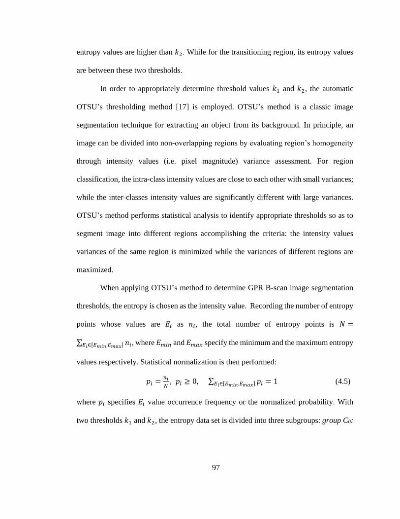
97

entropy values are higher than 𝑘2. While for the transitioning region, its entropy values

are between these two thresholds.

In order to appropriately determine threshold values 𝑘1 and 𝑘2, the automatic

OTSU’s thresholding method [17] is employed. OTSU’s method is a classic image

segmentation technique for extracting an object from its background. In principle, an

image can be divided into non-overlapping regions by evaluating region’s homogeneity

through intensity values (i.e. pixel magnitude) variance assessment. For region

classification, the intra-class intensity values are close to each other with small variances;

while the inter-classes intensity values are significantly different with large variances.

OTSU’s method performs statistical analysis to identify appropriate thresholds so as to

segment image into different regions accomplishing the criteria: the intensity values

variances of the same region is minimized while the variances of different regions are

maximized.

When applying OTSU’s method to determine GPR B-scan image segmentation

thresholds, the entropy is chosen as the intensity value. Recording the number of entropy

points whose values are 𝐸𝑖 as 𝑛𝑖, the total number of entropy points is 𝑁 =

∑ 𝑛𝑖𝐸𝑖∈[𝐸𝑚𝑖𝑛,𝐸𝑚𝑎𝑥] , where 𝐸𝑚𝑖𝑛 and 𝐸𝑚𝑎𝑥 specify the minimum and the maximum entropy

values respectively. Statistical normalization is then performed:

𝑝𝑖 =𝑛𝑖

𝑁, 𝑝𝑖 ≥ 0, ∑ 𝑝𝑖𝐸𝑖∈[𝐸𝑚𝑖𝑛,𝐸𝑚𝑎𝑥] = 1 (4.5)

where 𝑝𝑖 specifies 𝐸𝑖 value occurrence frequency or the normalized probability. With

two thresholds 𝑘1 and 𝑘2, the entropy data set is divided into three subgroups: group C0:

98

[𝐸𝑚𝑖𝑛, 𝑘1], group C1: (𝑘1, 𝑘2), group C2: [𝑘2, 𝐸𝑚𝑎𝑥]. The occurrence frequency of each

subgroup can be calculated as:

𝜔0 = 𝑃(𝐶0) = ∑ 𝑝𝑖𝐸𝑖∈[𝐸𝑚𝑖𝑛,𝑘1]

𝜔1 = 𝑃(𝐶1) = ∑ 𝑝𝑖𝐸𝑖∈(𝑘1,𝑘2) (4.6)

𝜔2 = 𝑃(𝐶2) = ∑ 𝑝𝑖𝐸𝑖∈[𝑘2,𝐸𝑚𝑎𝑥]

and the group mean values are:

𝜇0 = ∑ 𝐸𝑖𝑃(𝐸𝑖|𝐶0)𝐸𝑖∈[𝐸𝑚𝑖𝑛,𝑘1] = ∑ 𝐸𝑖𝑝𝑖

𝜔0𝐸𝑖∈[𝐸𝑚𝑖𝑛,𝑘1]

𝜇1 = ∑ 𝐸𝑖𝑃(𝐸𝑖|𝐶1)𝐸𝑖∈(𝑘1,𝑘2) = ∑ 𝐸𝑖𝑝𝑖

𝜔1𝐸𝑖∈(𝑘1,𝑘2) (4.7)

𝜇2 = ∑ 𝐸𝑖𝑃(𝐸𝑖|𝐶2)𝐸𝑖∈[𝑘2,𝐸𝑚𝑎𝑥] = ∑ 𝐸𝑖𝑝𝑖

𝜔2𝐸𝑖∈[𝑘2,𝐸𝑚𝑎𝑥]

The overall entropy mean equals

𝜇𝑇 = 𝜇(𝐿) = ∑ 𝐸𝑖𝑝𝑖𝐸𝑖∈[𝐸𝑚𝑖𝑛,𝐸𝑚𝑎𝑥] (4.8)

The intra-class variances can be calculated as

𝜎02 = ∑ (𝐸𝑖 − 𝜇0)2𝑃(𝐸𝑖|𝐶0)𝐸𝑖∈[𝐸𝑚𝑖𝑛,𝑘1] = ∑ (𝐸𝑖 − 𝜇0)2 𝑝𝑖

𝜔0𝐸𝑖∈[𝐸𝑚𝑖𝑛,𝑘1]

𝜎12 = ∑ (𝐸𝑖 − 𝜇1)2𝑃(𝐸𝑖|𝐶1)𝐸𝑖∈(𝑘1,𝑘2) = ∑ (𝐸𝑖 − 𝜇1)2 𝑝𝑖

𝜔1𝐸𝑖∈(𝑘1,𝑘2) (4.9)

𝜎22 = ∑ (𝐸𝑖 − 𝜇2)2𝑃(𝐸𝑖|𝐶2)𝐸𝑖∈[𝑘2,𝐸𝑚𝑎𝑥] = ∑ (𝐸𝑖 − 𝜇2)2 𝑝𝑖

𝜔2𝐸𝑖∈[𝑘2,𝐸𝑚𝑎𝑥]

The inter-class variance can be measured by the following discriminate criterion

𝜎𝐵2 = 𝜔0(𝜇0 − 𝜇𝑇)2 + 𝜔1(𝜇1 − 𝜇𝑇)2 + 𝜔2(𝜇2 − 𝜇𝑇)2 = 𝜔0𝜔1(𝜇0 − 𝜇1)2

+𝜔1𝜔2(𝜇1 − 𝜇2)2 + 𝜔2𝜔0(𝜇2 − 𝜇0)2 (4.10)

which is a function of threshold variables 𝑘1 and 𝑘2. The optimal thresholds 𝑘1∗ and 𝑘2

∗

can be determined by maximizing 𝜎𝐵2 [17]:

99

𝜎𝐵2(𝑘1

∗, 𝑘2∗) = max

𝑘1,𝑘2∈[𝐴𝑚𝑖𝑛,𝐴𝑚𝑎𝑥]𝜎𝐵

2(𝑘1, 𝑘2) (4.11)

The adoption of these two optimal thresholds can maximize inter-group entropy variance.

In the meantime, the intra-group entropy values variance is minimized [17].

4.3.4. Short Time Fourier Transform (STFT)

In essence, STFT implements local Fourier Transform on data that are evenly

divided into smaller time windows. Mathematically, STFT algorithm is expressed as

below:

𝑋(𝜏, Ω) = ∫ 𝑥(𝜏)𝑤(𝜏 − 𝑡)𝑒−𝑗Ω𝜏𝑑𝜏∞

−∞ (4.12)

where 𝑥 is the received GPR signal, Ω is the radial frequency whose resolution (∆Ω =

2𝜋 𝑁⁄ ) is determined by the number of points (𝑁) adopted for FFT computation. In this

analysis, 𝑁 = 256. 𝜏 is the time resolution. Since our GPR digitizer’s sampling

frequency is 8 Gsps, 𝜏 equals 125 ps. 𝑤(𝑡) is the window function. Here a Hamming

window is employed. In STFT analysis, there exists a tradeoff between time and

frequency resolution when determining the window size. Through a series of iterative

experiments, we select 1/10 the total number of time index to set the window size, which

is proven effective in achieving a good balance between frequency and time resolution

for rebar detection.

4.4. Experiment Results and Discussion

4.4.1. Rebar Test Results

Based on entropy and STFT characteristics analyzed above, this chapter proposes

to perform 2-D entropy analysis first to narrow down data scope to distinctive regions,

and then utilizes STFT to refine true singular region detection. For rebar in-air setup,

100

entropy analysis Eq. (4.3) with 𝛼 = 3 is first applied to B-scan image along Y-axis, as

shown in Figure 4.9. The obtained smooth entropy curve is plotted in Figure 4.9(b). Using

OTSU’s thresholding method, two threshold values 𝑘1∗ = 28.96 and 𝑘2

∗ = 31.08 are

calculated. The region between 0 and 𝑘1∗ is the singular region, while the region between

𝑘1∗ and 𝑘2

∗ is the transition region. In this study, in order not to miss detecting the areas

of interests, we take a conservative approach by searching for both the singular region

and the transition region, where both regions have entropy values below the higher

threshold 𝑘2∗ = 31.08. As illustrated in Figure 4.9(b), there are two regions whose

entropy values are below this threshold. One locates between 𝑡 = 1.625 ns and 5.75 ns

and the other one locates between 𝑡 = 7.75 ns and 8.625 ns.

Subsequently, Renyi’s entropy calculation is applied to scanning traces along X-

axis. Figure 4.10(b) plots the entropy curve. Using OTSU’s thresholding method, two

threshold values 𝑘3∗ = 10.25 and 𝑘4

∗ = 12.01 are obtained to identify the distinctive data

region in X-direction. Like the analysis along Y-axis, the region containing rebar

reflection information is within the region below threshold 𝑘4∗, which is found between

𝑥 = 0.55 m and 𝑥 = 1.95 m.

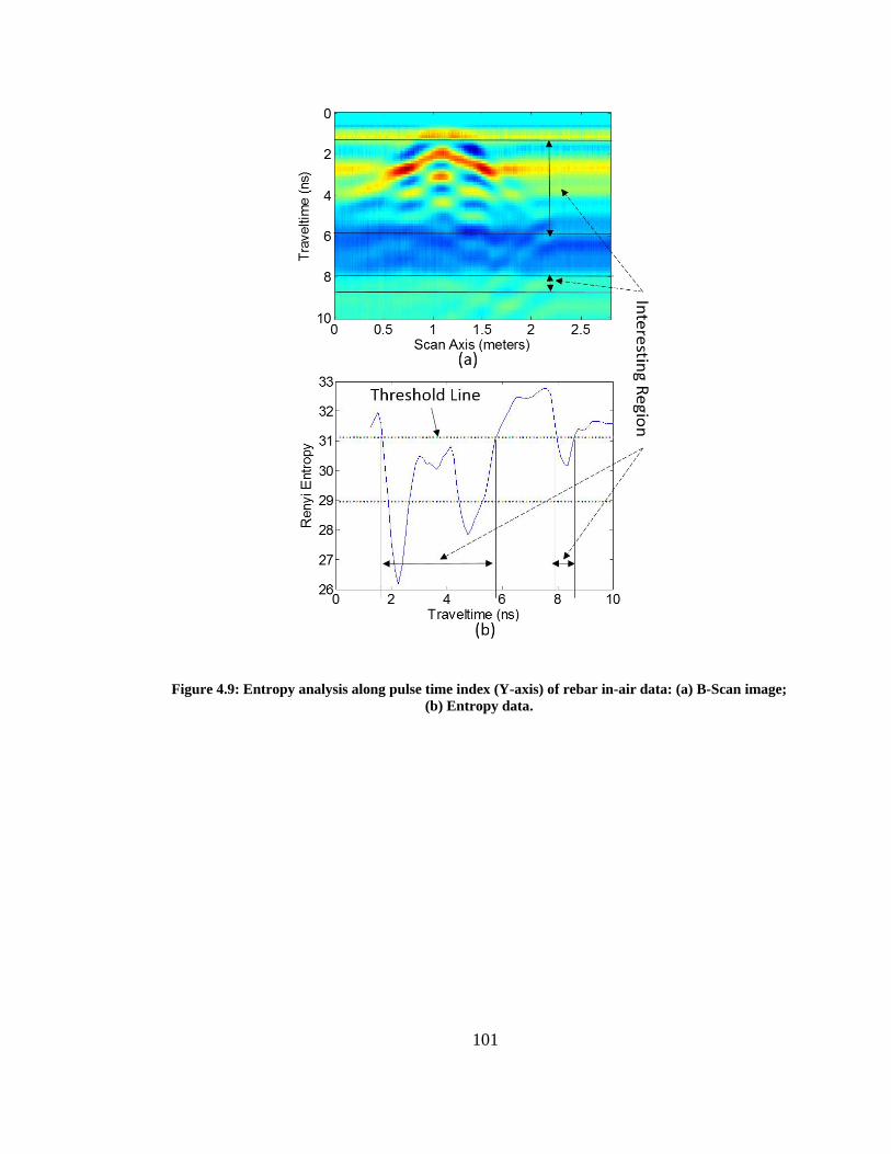
101

Figure 4.9: Entropy analysis along pulse time index (Y-axis) of rebar in-air data: (a) B-Scan image;

(b) Entropy data.

102

Figure 4.10: Entropy analysis along trace index (X-axis) of rebar in air B-scan: (a) B-Scan image;

(b) Entropy data.

By combining both x-axis and y-axis entropy analysis results, the intersection

regions are obtained. For rebar-in-air setup, the extracted regions are illustrated in Figure

4.11(a); while for rebars-in-concrete-slab setup, the extraction regions are highlighted in

Figure 4.11(b). In both cases, a false region below 7 ns is also extracted. STFT analysis

is then performed to refine the extraction result and eliminate the false region.

103

Figure 4.11: 2D entropy analysis for B-scan images of a) rebar in air and b) rebars in concrete.

For one-rebar-in-air data, STFT analysis is performed on the selected signal trace

at 𝑥 = 1.1 m across the extracted regions in Figure 4.11(a). The obtained time-spectrum

is plotted in Figure 4.12(a). As shown, no strong reflection occurs between 8 ns and 10

ns, which means the second region (8 ns ~ 9 ns) in Figure 4.11(a) is the false singular

region that should be eliminated. The corrected singular region extraction result is plotted

in Figure 4.13(a). Similarly for two-rebar in concrete slab data, STFT analysis on the

signal trace locating at x=1.5m is performed and the result is displayed in Figure 4.12(b).

As shown, no strong reflection exists between 6 ns and 10 ns, which indicates the second

region (between 7 ns and 9 ns) in Figure 4.11(b) is also a false region and should be

eliminated. The corrected singular region extraction result is displayed as Figure 4.13(b).

In both cases, the extracted rebar region comprises less than 40% of the entire scanning

data volume.

104

Figure 4.12: STFT analysis to correct the singular region detection: (a) STFT result of one rebar

data at x=1.1m; (b) STFT result of two rebar data at x=1.5m.

Figure 4.13: Final singular region for B-scan images of a) rebar in air and b) two rebars in

concrete.

Further, STFT is operated on trace signals selected from the left side, the middle,

and the right side of the rebar region respectively. The corresponding STFT analysis

results are shown in Figure 4.14(b), Figure 4.14(c), and Figure 4.14(d).

105

Figure 4.14: (a) Rebar in air B-scan image; 2D entropy and STFT analysis results of traces at (b)

left side, (c) middle and (d) right side of rebar area.

In Figure 4.14(b), a strong peak occurs at 2.8 ns on the trace of 𝑥 = 0.75 m when

antennas are on the left side. Figure 4.14(c) shows when the antennas are right above the

rebar (the trace of 𝑥 = 1.1 m), a strong peak pulse is produced at 1.9 ns. Figure 4.14(d)

depicts a strong peak at 2.8 ns on trace of 𝑥 = 1.5 m when antennas are on the right side.

In our experiments, we are able to find out that the 2.8 ns peak pulse is the reflection

signal from the floor surface underneath rebar with the utilization of a large metal sheet.

By covering the floor surface with a large metal sheet, a stronger reflection pulse is

observed occurring at exactly the same time instant (2.8 ns), which validates the floor as

the reflection source. With reference to Figure 4.4(a), the distance between antennas and

106

the rebar can be determined through the following calculations: (1) Subtracting the time

offset between antennas direct coupling pulse (𝑡 = 0.5 ns) (The transmitter antenna and

receiver antenna are packed together inside of a box, the direct coupling pulse time is

thus used as the reference time point) and the strongest STFT peak point (𝑡 = 1.9 ns),

obtains time offset ∆𝑡 = 1.4 ns; (2) Inserting ∆𝑡 to the following equation

𝑉 = 𝑑/(Δ𝑡

2) (4.13)

where 𝑑 is the distance, 𝑉 is the speed of light in air (3x108 m/s), and (∆𝑡/2) indicates

one way signal travel time from rebar to the receiver antenna. The distance 𝑑 is thus

calculated to be 210 mm, which agrees well with the physical setup described in section

4.2.1, where antennas are placed 220 mm above the rebar.

For two rebars in a concrete slab setup, Figure 4.15(a) extracts the intersected B-

scan image section that focuses on rebars. Both STFT images of the left side trace (the

trace at 𝑥 = 1.25 m) (Figure 4.15(b)) and right side trace (the trace at 𝑥 = 1.7 m) (Figure

4.15(c)) show two strong peaks (in red color) at 1.75 ns and 3.125 ns. These peak time

values are used to compute rebars burying depths inside the concrete slab. The radar

signal two-way travel time between concrete and rebars is calculated to be 3.125 ns –

1.75 ns = 1.375 ns. The electromagnetic (EM) wave travel velocity 𝑉𝑐 inside concrete

needs to be taken into account, which equals:

𝑉𝑐 = 𝑉/√𝜀𝑐 (4.14)

𝜀𝑐 is the relative dielectric constant of the concrete which equals about 4.1 according to

our measurements conducted in [18], [19], [20] and [21]. 𝑉 is the speed of light in air. 𝑉𝑐

is calculated to be 1.48x108 m/s. Using Eq. (4.13) with ∆𝑡 = 1.375 ns, the rebar burying

107

depth from concrete surface is computed to be 102 mm approximately, which is in good

agreement with the physical setups (98.6/108 mm depths) described in Section 4.2.

Figure 4.15: (a) Rebars in concrete B-scan image; 2D entropy and STFT analysis at (b) left rebar

and (c) right rebar.

108

4.4.2. Ballast Test Results

Figure 4.16: Entropy analysis of ballast data: (a) Entropy along Travel time index (Y-axis); (b)

Entropy along Scan Axis (X-axis).

For ballast platform setup, entropy analysis is first applied to the B-scan image

along Y-axis, as shown in Figure 4.16(a). Using OTSU’s thresholding method, two

threshold values 𝑘1∗ = 5.08 and 𝑘2

∗ = 5.92 are calculated. The singular regions have

entropy values below threshold 𝑘1∗. As illustrated in Figure 4.16(a), there are three regions

whose entropy values are below this threshold. The first one locates between 𝑡 = 5.125

109

ns and 6.00 ns, the second locates between 𝑡 = 11.00 ns and 12.50 ns, and the third one

locates between 𝑡 = 14.25 ns and 17.50 ns.

Subsequently, Renyi’s entropy is computed along X-axis. Figure 4.16(b) plots the

obtained curve. Using OTSU’s thresholding method, two threshold values 𝑘3∗ = 4.88 and

𝑘4∗ = 5.43 are obtained. Similar to the analysis along Y-axis, the singular region is below

threshold 𝑘3∗, which locates between 𝑥 = 2.35 m and 𝑥 = 2.75 m. By combining both

the x-axis and y-axis entropy analysis results, the intersection regions in the B-scan image

are obtained. For the ballast platform setup, the extracted region is illustrated in Figure

4.17.

Figure 4.17: 2-D entropy analysis for B-Scan image of ballast platform.

To refine region identification, windowing STFT analysis is performed on a trace

signal across three regions locating at 𝑥 = 2.5 m. The corresponding STFT analysis

result is shown in Figure 4.18.

110

Figure 4.18: STFT analysis result of trace at x = 2.5 m.

As shown in Figure 4.18, a strong peak occurs only between 11 ns and 12 ns. This

result indicates that region 2 in Figure 4.17 is the true singular region while regions 1 and

3 are false ones. Combining the results of entropy analysis and STFT analysis, the correct

fouled ballast region is singled out in Figure 4.19. In this test case, the extracted region

comprises less than 5% of the entire scanning data volume.

Figure 4.19: Final moisture region detection result based on entropy and STFT analysis.

111

To validate the detection result, the fouled ballast region depth is computed in a

similar way as the rebar test. The ground surface reflection signal locates at 𝑡 = 8.5 ns

in Figure 4.6(a), and the detected region top side locates at 𝑡 = 11.0 ns, therefore the

two-way travel time of radar incident signal between ground surface and moisture region

is 11.0 ns – 8.5 ns = 2.5 ns. Substituting the measured dielectric constant of clean ballast

𝜀𝑐 = 3 into Eq. (4.14), 𝑉𝑐 is calculated as 1.73x108 m/s. Using Eq. (4.13) with ∆𝑡 = 1.25

ns, the depth of the fouled ballast region is computed as 0.216 m approximately. This

value agrees well with the actual physical setups (0.2 m depth).

4.5. Conclusions

This chapter has demonstrated the integration of 2D entropy and STFT analytical

methods to leverage GPR data processing efficiency. By computing radargram 2D

entropy and OTSU’s thresholds, singular areas within large background data can be

effectively extracted. The utilization of entropy analysis effectively reduces the data

volume for implementing more sophisticated post-processing algorithms. In our test

experiments, around 60% data compression rate is achieved for rebar detection and 95%

data compression rate is achieved for fouled ballast region detection. STFT is then

applied for time-frequency characterization to leverage region detection accuracy and

screen out false results. Note there are other more sophisticated JTF analysis methods,

such as Gabor transform, wavelet, fractional Fourier transform, etc., that are capable of

more advanced characterizations when the data scope is more focused with the assistance

of entropy calculation. STFT is generally sufficient for these applications that require

marginal detection resolutions.

112

4.6. References

[1] Z.W. Wang, M. Zhou, G.G. Slabaugh, J. Zhai, and T. Fang, “Automatic Detection

of Bridge Deck Condition From Ground Penetrating Radar Images,” IEEE

Transactions on Automation Science and Engineering, Vol. 8, No. 3, pp 633-640,

2011

[2] F. Soldovieri, R. Solimene, L. Lo Monte, M. Bavusi, and A. Loperte, “Sparse

Reconstruction From GPR Data With Applications to Rebar Detection,” IEEE

Transactions on Instrumentation and Measurement, Vol. 60, No. 3, pp. 1070-1079,

2011

[3] V. Krause, I. Abdel-Qader, O. Abudayyeh , and S. Yehia, “An Image

Segmentation Algorithm for the Detection of Rebar in Bridge Decks from GPR

Scans,” Proceedings of IEEE International Conference on Electro/Inforation

Technology, Vol. 7, 2007, pp 114-119.

[4] A. Simi, G. Manacorda, and A. Benedetto, “Bridge deck survey with high

resolution Ground Penetrating Radar,” 14th International Conference on GPR,

2012, pp 489-495.

[5] J.S. Lee, C. Nguyen, and T. Scullion, “A Novel, Compact, Low-Cost, Impulse

Ground-Penetrating Radar for Nondestructive Evaluation of Pavements,” IEEE

Transactions on Instrumentation and Measurement, Vol. 53, No. 6, pp1502-1509,

2004

[6] W.L. Lai, C.S. Poon, “GPR data analysis in time-frequency domain,” 14th

International Conference on GPR, 2012, pp 362-366.

[7] https://www.princeton.edu/~achaney/tmve/wiki100k/docs/Entropy_%28informat

ion_theory%29.html

[8] W. Zhi and F. Chin, “Entropy-Based Time Window for Artifact Removal in UWB

Imaging of Breast Cancer Detection,” IEEE Signal Processing Letters, Vol. 13,

No. 10, 2006, pp 585-588.

[9] M. Ferrario, M. G. Signorini, G. Magenes, and S. Cerutti, “Comparison of

Entropy-Based Regularity Estimators: Application to the Fetal Heart Rate Signal

for the Identification of Fetal Distress,” IEEE Transactions on biomedical

engineering, Vol. 53, No. 1, pp 119-125, 2006

[10] H. You, Q. Zhu, and A. Alwan. “Entropy-based variable frame rate analysis of

speech signals and its application to ASR,” IEEE Acoustics, Speech, and Signal

Processing, 2004, Vol.1, pp 549-52.

[11] E.C. Kenley and Y-R Cho, “Entropy-Based Graph Clustering: Application to

Biological and Social Networks,” IEEE International Conference Data Mining,

2011, pp 1116-1121

[12] R. Solimene and A. Cuccaro, "Front Wall Clutter Rejection Methods in TWI,"

Geoscience and Remote Sensing Letters, IEEE , vol.11, no.6, pp.1158,1162, June

2014

https://www.princeton.edu/~achaney/tmve/wiki100k/docs/Entropy_%28information_theory%29.html

https://www.princeton.edu/~achaney/tmve/wiki100k/docs/Entropy_%28information_theory%29.html

113

[13] M. Hanmandlu, O.P. Verma, N.K. Kumar, and M. Kulkarni, “A Novel Optimal

Fuzzy System for Color Image Enhancement using Bacterial Foraging,” IEEE

Transactions on Instrumentation and Measurement, vol. 58, no. 8, 2009, pp 2867-

2879.

[14] T. P. Zielinski, “Joint Time-Frequency Resolution of signal Analysis Using Gabor

Transform,” IEEE Transactions on Instrumentation and Measurement. vol. 50,

No. 5. 2001. pp. 1436-1444.

[15] Z. Li and M. J. Crocker, “A Study of Joint Time-Frequency Analysis-Based

Modal Analysis,” IEEE Transactions on Instrumentation and Measurement. vol.

55, No. 6. 2006. pp. 2335-2342.

[16] P. Candra, T. Xia, D. Huston, and G.A. Wang, "Two dimensional entropy and

short time Fourier Transform application on ground penetrating radar data

analysis," Proc. SPIE 8694, Nondestructive Characterization for Composite

Materials, Aerospace Engineering, Civil Infrastructure, and Homeland Security

2013, 86940J (April 24, 2013); doi:10.1117/12.2010224.

[17] N. Otsu, “A Threshold Selection Method from Gray-Level Histograms,” IEEE

Transactions on Systems, Man and Cybernetics, vol. 9, Issue: 1, 1979, pp 62 – 66.

[18] A. Venkatachalam, X.L. Xu, D. Huston, and T. Xia, "Development of a New High

Speed Dual-Channel Impulse Ground Penetrating Radar," IEEE Journal of

Selected Topics in Applied Earth Observations and Remote Sensing. Vol. 6, No.

6, Dec. 2013.

[19] T. Xia, XL. Xu, A. Venkatachalam, and D. Huston, "Development of a High Speed

UWB GPR for Rebar Detection," Proceedings of IEEE International Conference

on Ground Penetrating Radar (GPR) 2012.

[20] T. Xia, A. S. Venkatachalam, and D. Huston, "A High Performance Low Ringing

Ultra-Wideband Monocycle Pulse Generator," IEEE Transactions on

Instrumentation and Measurement. vol. 61, Issue 1. 2012. pp. 261-266.

[21] X.L. Xu, T. Xia, A. Venkatachalam, and D. Huston, “Development of High-Speed

Ultrawideband Ground-Penetrating Radar for Rebar Detection,” Journal of

Engineering Mechanics, vol. 139, no. 3, 2012, pp 272-285.

[22] R. G. Baraniuk, P. Flandrin, A. J. E. M. Janssen, and O. Michel, “Measuring time-

frequency information content using the Rényi entropies,” IEEE Trans. Inf.

Theory, vol. 47, no. 4, May 2001, pp. 1391–1409.

[23] S. W. Smith, “The Scientist and Engineer's Guide to Digital Signal Processing,”

Second Edition, California Technical Publishing, San Diego, 1999.

114

CHAPTER 5: GROUND PENETRATING RADAR RAILROAD BALLAST

INSPECTION WITH AN UNSUPERVISED ALGORITHM TO BOOST THE

REGION OF INTEREST DETECTION EFFICIENCY

Abstract

Railroad ballast inspection is critical for the safety of both passenger and freight

rail. Ground penetrating radar (GPR) has been utilized as a highly efficient non-

destructive evaluation (NDE) and structural health monitoring technique in bridge and

roadway inspection for many years. However, the development of robust GPR

technologies for railroad ballast inspection is still at its early stage due to the complex

scattering characteristics of ballast and the lack of efficient algorithms to process big

GPR data. In this study, an efficient unsupervised method for detecting the region of

interest in ballast layer based on Hilbert Transform and Renyi entropy analysis is

proposed and tested extensively using an indoor platform emulating the railroad

structure. Based on the lab test results, this unsupervised analysis approach is utilized to

characterize 300 GB field test data collected at Massachusetts Bay Transit Authority

(MBTA) and Metro St. Louis. The data interpretation results demonstrate that the

developed region of interest detection algorithm is an efficient and valuable tool for GPR

data processing.

Keywords: ground penetrating radar, information entropy, Hilbert transform, railroad

ballast inspection, automatic detection, region of interest.

115

5.1. Introduction

Typical railroad subsurface defects include cavity, fouled ballast, high degree of

moisture, etc. Although railroad subsurface structure safety is critical, its inspection is

very challenging. Traditional inspection methods such as drilling test and

acoustic/hammer test are either destructive or inefficient, labor intensive, time

consuming, disturbing to the normal traffic, etc. As a non-destructive and highly efficient

test method, GPR has been widely used for concrete bridge decks inspection [1], asphalt

pavement monitoring [2], highway rebar detection [3], railroad ballast condition

assessment [4], soil moisture estimation [5], etc. Among these applications, railroad

ballast condition assessment is especially challenging due to the complex scattering

characteristics of the ballast. Although a number of studies have been conducted, the

application of GPR for railroad structure inspections is still in its early stage.

For applying GPR to railroad inspections, a major challenge is how to effectively

process and interpret GPR data. There are sophisticated processing algorithms [6]-[9]

that can effectively characterize subsurface structural features. Sparse representation is

utilized in Ref. [6] to extract the feature of the A-Scan trace signal, and Support Vector

Machine (SVM) technique [7] is applied for the GPR A-Scan traces classification based

on a prior knowledge. Discrete wavelet transform is used in Ref. [8] to extract the texture

feature in GPR B-Scan image and similarity measurement is performed to compare the

tested B-Scan image and known B-Scan image pattern for ballast of various fouling

condition. Similarly, discrete wavelet transform and fractional Fourier transform [9] are

developed to extract features of each GPR A-Scan trace, and these features are supplied

116

to SVM classifiers to identify the underground objects. Nearly all existing GPR ballast

data interpretation methods share the same data processing scheme: 1. producing priori

knowledge about various fouling ballast patterns; 2. applying the feature extraction

method to GPR data to extract test patterns; 3. using a classifier to categorize the test data

in accordance to fouling ballast patterns.

Such supervised methods can achieve high classification accuracy, however they

are computationally complex. For large scale GPR survey, the collected inspection data

is typically over hundred Giga Bytes (GB), making the direct application of these

sophisticated data processing methods difficult and sometimes even infeasible. On the

other hand, the structural composition of field ballast layer is very complex as some other

scatters or material can be mixed within the ballast. Even the prior knowledge can be

obtained using some ballast test with various fouling conditions, the feature pattern of

field test ballast cannot be guaranteed to exist in the known training pattern due to its

complex material composition. Therefore, developing an unsupervised and automatic

GPR data processing method that can effectively and rapidly identify suspicious features

from big radargram is critically desirable, which will facilitate advanced radar data post

processing, such as the sophisticated feature extraction and pattern recognition.

In our previous work, an entropy analysis and short-time Fourier transform

(STFT) based unsupervised algorithm has been developed and demonstrated to boost

GPR signal processing efficiency [10]. By computing radargram 2D entropy and OTSU’s

thresholds, singular areas within large background data can be effectively extracted. The

utilization of entropy analysis effectively reduces the data volume for implementing more

117

sophisticated post-processing algorithms. STFT performs time-frequency

characterization to leverage region detection accuracy and screen out false results.

In this chapter, the customized entropy-based algorithm is improved to automate

and facilitate the detection of suspicious fouling ballast regions or Regions of Interest

(ROI) within big GPR survey data sets. Considering the GPR transmitting signal is a high

order (2nd order or higher) Gaussian pulse, the backscattering A-scan signal shows

multiple peaks, which increases the difficulty to identify the feature of scatters. In this

research, an analytic method using Hilbert Transform is developed to extract the pulse

signal envelope so as to characterize the scattering signal power. Furthermore, an

automatic layer identification method based on signal decomposition is implemented to

detect and isolate the ballast region from the ground surface. Finally, the 2D entropy

analysis is performed on the scattering data corresponding to ballast region. Such data

processing approaches leverage 2D entropy analysis effectiveness and eliminate the need

of STFT for singular region identification, so as to facilitate large volume GPR ballast

inspection data post processing and interpretation.

To validate data processing effectiveness, extensive laboratory experiments are

first conducted employing our Ultra Wideband (UWB) air-coupled impulse GPR system

[11]. Further analysis is conducted on large volume (overall 20 miles) railroad field test

data sets collected during the field test at Metro St. Louis and Massachusetts Bay Transit

Authority (MBTA).

118

5.2. GPR System Configuration

In this chapter, the experimental data are collected with our air-coupled impulse

GPR system developed in Ref. [3], [11] and [12]. Figure 5.1 illustrates the system

diagram. As shown in Figure 5.1, the GPR system hardware consists of five major

functional units: (1) RF transmitter; (2) Ultra-wideband antennas; (3) Data acquisition

unit comprising of a high speed real time digitizer, high speed data transmission and

storage unit; (4) Quard-core computer (Intel core i7 3.4 GHz) (5) FPGA digital controller

along with a wheel encoder.

Figure 5.1: GPR system diagram: (a) High Speed UWB GPR System; (b) Digitizer Configured in

SAR Mode; (c) UWB Pulse Generator; (d) UWB Antenna.

The RF transmitter comprises a UWB pulse generator that generates high-

amplitude Gaussian pulses with the Pulse Repetition Frequency (PRF) controlled by the

119

FPGA. The high-speed digitizer contains a 10-bit 8 GSPS real-time sampling Analog-to-

Digital Converter (ADC), which also includes a high-throughput data transmission unit

connected to the multi-core computer via Peripheral Component Interconnect express

(PCIe) bus. The computer streams the GPR data from the digitizer and tags the data with

header information. The optical encoder measures the travel distance and generates

quadrature pulses correspondingly. The FPGA receives the wheel encoder pulses and

triggers GPR scans. The travel distance information is transmitted to the computer for

data location registration. The antennas have a compact size and good impedance

matching over a wide bandwidth from 600 MHz to 6 GHz for effective signal

transmission and reception. Some selected key specifications of this GPR system are

summarized in Table 1.1.More design details are elaborated in Ref. [3], [11]-[13].

Table 5.1: Air-coupled Impulse GPR System Specifications.

Data acquisition unit 8 Gsps, 10-bit resolution

GPR reflection pulse

sampling window width 40 ns

Pulse repetition frequency 0 to 30 kHz tunable

Horizontal resolution 1 cm at 100 km/h survey speed

Signal bandwidth 600 MHz to 2 GHz tunable

Penetrating capability Up to 1 meter

120

5.3. Unsupervised GPR ROI Detection Method

The flow chart of the proposed unsupervised GPR signal processing methods for

detecting region of interest is illustrated in Figure 5.2. Stacking and low pass filtering are

first performed on raw B-scan image for noise reduction. Hilbert transform is then

utilized to extract the scattering signal envelope and characterize the signal power, based

on which, the A-Scan decomposition is conducted to identify interfacing layers between

different materials and to locate the ballast region for data interpretation. Clutter removal

and stacking are then performed to enhance the ballast region image. Finally, the

statistical 2D entropy analysis is applied to quickly detect the singular region of interest.

Details of each step are elaborated in the following subsections.

Raw DataStacking Every

50 TracesLow Pass Filter

Hilbert Transform

A-Scan Decomposition

Ballast Region Identification

Clutter RemovalStacking Every

10 Traces2D Entropy

AnalysisRegion of Interest

Pre-processing Power Information Characterization

Ballast Region Identification

B-Scan Image EnhancementRegion of Interest Dection

Figure 5.2: Unsupervised algorithm for detecting region of interest in ballast layer.

5.3.1. Pre-processing

To enhance the raw B-Scan images quality, a two-step pre-processing is

implemented:

Step 1: Stack every 50 A-scan traces to calculate the average to boost the signal-

to-noise ratio (SNR) [14].

121

The GPR signal transmitter is triggered in distance. The perimeter of the hi-rail

SUV wheel used in GPR test is 0.77 m, and the wheel encoder has 10000 triggers per

rotation. Thus, the distance interval between two pulses are 0.77m/10000 = 0.077 mm.

Stacking every 50 traces results in 0.077mm*50 = 3.85 mm distance interval between

two pulses, which assures the good spatial scanning resolution as well as improves the

SNR of GPR A-Scan trace.

Step 2: Apply Low Pass Filtering (LPF) with a 2 GHz cutoff frequency. In the

test, our GPR pulse signal spectrum is tuned as a monocycle pulse with 1 GHz center

frequency, and the amplitude spectrum of received GPR A-Scan trace is shown in Figure

5.3. A 2 GHz LPF is employed to filter out the out-of-band high frequency noise.

Figure 5.3: Amplitude spectrum of GPR A-Scan trace.

0 1 2 3 40

1000

2000

3000

4000

5000

6000Amplitude Spectrum of GPR signal

Frequency (GHz)

Am

plit

ud

e S

pe

ctr

um

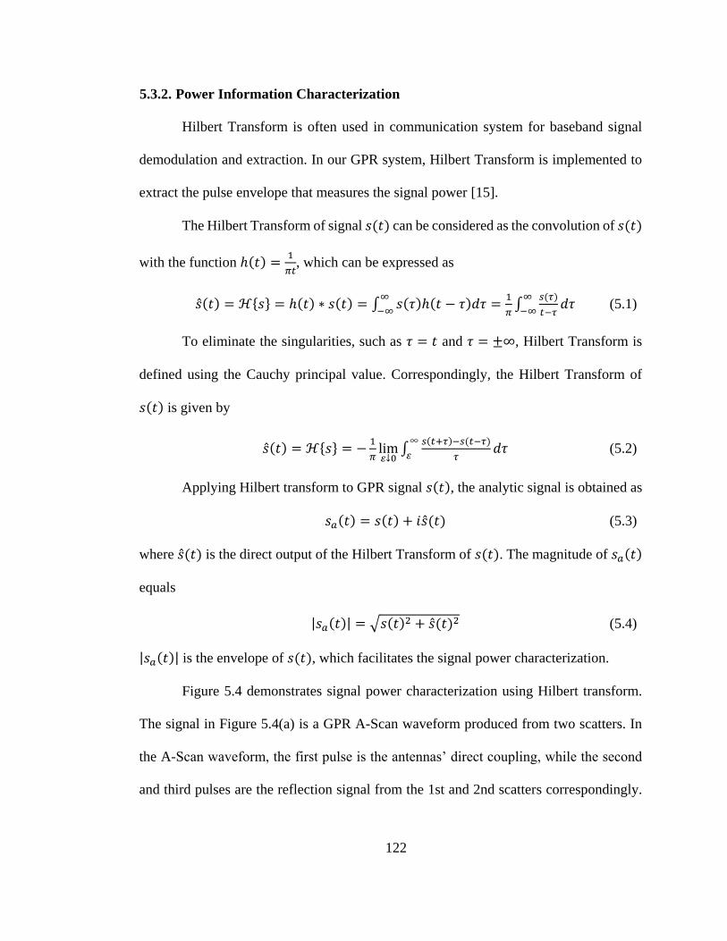
122

5.3.2. Power Information Characterization

Hilbert Transform is often used in communication system for baseband signal

demodulation and extraction. In our GPR system, Hilbert Transform is implemented to

extract the pulse envelope that measures the signal power [15].

The Hilbert Transform of signal 𝑠(𝑡) can be considered as the convolution of 𝑠(𝑡)

with the function ℎ(𝑡) =1

𝜋𝑡, which can be expressed as

�̂�(𝑡) = ℋ{𝑠} = ℎ(𝑡) ∗ 𝑠(𝑡) = ∫ 𝑠(𝜏)ℎ(𝑡 − 𝜏)𝑑𝜏∞

−∞=

1

𝜋∫

𝑠(𝜏)

𝑡−𝜏𝑑𝜏

∞

−∞ (5.1)

To eliminate the singularities, such as 𝜏 = 𝑡 and 𝜏 = ±∞, Hilbert Transform is

defined using the Cauchy principal value. Correspondingly, the Hilbert Transform of

𝑠(𝑡) is given by

�̂�(𝑡) = ℋ{𝑠} = −1

𝜋lim𝜀↓0

∫𝑠(𝑡+𝜏)−𝑠(𝑡−𝜏)

𝜏𝑑𝜏

∞

𝜀 (5.2)

Applying Hilbert transform to GPR signal 𝑠(𝑡), the analytic signal is obtained as

𝑠𝑎(𝑡) = 𝑠(𝑡) + 𝑖�̂�(𝑡) (5.3)

where �̂�(𝑡) is the direct output of the Hilbert Transform of 𝑠(𝑡). The magnitude of 𝑠𝑎(𝑡)

equals

|𝑠𝑎(𝑡)| = √𝑠(𝑡)2 + �̂�(𝑡)2 (5.4)

|𝑠𝑎(𝑡)| is the envelope of 𝑠(𝑡), which facilitates the signal power characterization.

Figure 5.4 demonstrates signal power characterization using Hilbert transform.

The signal in Figure 5.4(a) is a GPR A-Scan waveform produced from two scatters. In

the A-Scan waveform, the first pulse is the antennas’ direct coupling, while the second

and third pulses are the reflection signal from the 1st and 2nd scatters correspondingly.

123

As the transmitting pulse signal is the Ricker wavelet (the second order derivatives of

Gaussian function), the backscattering pulse from each object or layer interface shows

three peaks. Figure 5.4(b) shows the waveform produced by the Hilbert transform where

the three peaks become much more discernible.

Figure 5.4: Hilbert transform for signal power characterization: (a) GPR A-Scan trace; (b) GPR

A-Scan envelope.

5.3.3. Identification of Ballast Region

Prior to 2D entropy analysis, an A-Scan decomposition is performed to remove

clutters that are produced due to various sources, such as antenna direct coupling, cross-

ties reflection, etc, and to isolate ballast layer for more sophisticated post processing.

For signal decomposition, the transmitter and receiver antennas’ direct coupling

pulse is utilized as the reference signal which preserves the transmitted pulse signal

shape. Cross-correlation is a measure of similarity of two signal sequences as a function

of the lag of one relative to the other. Denoting the reference GPR A-Scan trace as 𝑓[𝑡]

124

and the target GPR A-Scan trace as 𝑔[𝑡], the cross-correlation for these two real signal

sequences is defined as:

𝐶𝑟𝑜𝑠𝑠𝐶𝑜𝑟(𝑓, 𝑔)[𝜏] ≝ ∑ 𝑓[𝑡]𝑔[𝑡 + 𝜏]∞𝑡=−∞ (5.5)

The scattering is located at the time shift 𝜏 which is determined as

𝜏 = 𝑎𝑟𝑔 max𝜏

|𝐶𝑟𝑜𝑠𝑠𝐶𝑜𝑟(𝑓, 𝑔)[𝜏]| (5.6)

By performing iterative cross correlations [16], an A-Scan waveform is

decomposed into the combinations of multiple pulses of varying amplitude and phases

characterizing the reflection signals from different scatters (i.e. objects or layers). Based

on the decomposition result, the signal component corresponding to the ballast layer is

picked out and the scope of data analysis is narrowed down to the ballast region.

Figure 5.5 demonstrates the process of A-Scan decomposition. In Figure 5.5(a),

the direct coupling signal with amplitude 𝐴1 at time instance 𝑡1 is chosen as the reference

signal. As shown in Figure 5.5(b), by performing cross correlation between the reference

signal and the A-Scan trace following 𝑡1 time instant, a maximum correlation value is

identified at time instance 𝑡2 which corresponds to the first backscattering pulse.

Continuing the cross correlation calculation, another backscattering pulse is identified at

time instance 𝑡3 as shown in Figure 5.5(c). Finally, the A-Scan trace is decomposed into

combinations of three pulses of varying amplitudes and time delays.

125

Figure 5.5: Signal decomposition for identification of backscattering from different sources: (a)

Direct coupling signal; (b) 1st backscattering pulse; (c) 2nd backscattering pulse.

5.3.4. B-Scan Image Enhancement

Upon ballast region identification, the resultant B-Scan image is further

enhanced:

Step 1: Remove the background signals (i.e. air-ground surface reflection signals)

using a 2-Dimensional (2D) High Pass Filter (HPF) [17]-[18]. The basic principle of this

filtering is that in the B-scan image’s horizontal direction, the frequency bandwidth of

the background clutter is much narrower than that of subsurface scattering signals.

Step 2: After clutter removal, every 10 A-scan traces are grouped to perform the

averaging calculation to further improve signal SNR as well as reduce data volume and

redundancy.

5.3.5. Entropy Based Region of Interest (ROI) Detection

Our automatic ROI detection method computes 2D Renyi entropy to characterize

data singularity so as to effectively identify and detect the structural features of interest.

126

In information theory, entropy is a measure of the uncertainty associated with a random

variable. For our GPR data processing, entropy characterization is explored to identify

singular regions within a large data set. In particular, a high entropy value indicates high

degree of data similarity while a low entropy value specifies high degree of data

singularity.

The received GPR backscattering signal 𝑌(𝑡) can be modeled with the following

equation:

𝑌(𝑡) = 𝐷(𝑡) + 𝑆(𝑡) (5.7)

where 𝐷(𝑡) represents the reflection signal from objects of interest, and 𝑆(𝑡) models

background signals, clutters or other interference signals. For entropy analysis, a power

normalization is first performed which can be expressed as

𝑦𝑖(𝑡) =‖𝑌𝑖(𝑡)‖2

∑ ‖𝑌𝑖(𝑡)‖2𝑀𝑖=1

(5.8)

where 𝑦𝑖(𝑡) is the normalized signal, 𝑖 denotes the trace index, 𝑀 is the total number of

traces included, and 𝑡 specifies the time index of data points on each reflection trace

waveform. Upon the power normalization, a generalized Renyi’s entropy [19] is

computed to assess the data singularity as:

𝐸𝛼(𝑡) =1

1−𝛼loge⟨∑ [𝑦𝑖(𝑡)]𝛼𝑀

𝑖=1 ⟩ (5.9)

where 𝐸𝛼(𝑡) is the entropy quantification and 𝛼 is the entropy order. Based on the study

in Ref. [10], 𝛼 = 3 can accomplish optimal performance.

Fouled ballast mixed with sand and fouled ballast of diverse moisture levels

produce distinct features of reflection [15], which can be characterized from entropy data

127

values for detecting the singular data regions. Following this idea, an automatic ROI

detection method is developed, which consists of the following data processing steps:

Step 1: 2D Renyi entropy calculations in accordance to Eq. (5.9).

Step 2: Entropy curve smoothing using a moving average method [20].

𝐸𝑠𝑚𝑜𝑜𝑡ℎ(𝑛) =1

𝑚∑ 𝐸(𝑖)𝑛

𝑖=𝑛−𝑚+1 (5.10)

In Eq. (5.10), 𝐸(𝑖) denotes the entropy value of index 𝑖 in entropy data sequence.

The moving average method calculates the mean of every 𝑚 data points to eliminate

noise and smooth out the entropy data array. In our analysis, 𝑚 is selected as 5% of the

total number of entropy data points to accomplish optimal smoothing performance as

well as preserve the data resolution.

Step 3: Adaptive entropy threshold determination using OTSU’s method.

Depending on the data characteristics, regions in a B-scan image can be classified

into three categories: singular region, stationary background region and the transition

region. The classification of a region can be done through assessing its entropy values

against two thresholds 𝐾1 and 𝐾2 (𝐾1 < 𝐾2). Singular regions have entropy values lower

than threshold 𝐾1, and stationary background regions have entropy values higher than

𝐾2. For transition regions, their entropy values are amid of these two thresholds. In order

to appropriately determine threshold values 𝐾1 and 𝐾2, the automatic OTSU’s

thresholding method [21] is employed. OTSU’s method is a classic image segmentation

technique for extracting an object from its background. In principle, an image can be

divided into non-overlapping regions by evaluating region’s homogeneity through

intensity values (i.e. pixel magnitude) variance assessment. For region classification, the

128

intra-class intensity values are close to each other with small variances; while the inter-

classes intensity values are significantly different with large variances. OTSU’s method

performs statistical analysis to identify appropriate thresholds so as to segment image

into different regions accomplishing the criteria: the intensity values variances of the

same region is minimized while the variances of different regions are maximized.

5.4. Lab Experiment

5.4.1. Test Configuration

To test and verify our automatic ROI region detection method, a test platform is

produced emulating a railroad segment as shown in Figure 5.6(a). The test platform is

3.5 meters long, 1.2 meters tall and 1.5 meters wide. It is filled with sand and ballast. One

portion of the ballast region is filled with the fouled ballast mixed with sand and water.

Figure 5.6(b) illustrates the platform structure: (1) The ballast layer of 0.3 meters

thickness is laid above the soil; (2) 0.75 meters apart from the left end of the platform,

an area (highlighted in blue) of 0.45 meters length and 0.2 meters depth is filled with the

fouled ballast, which is a mixture of sand, ballast, and water. This fouled ballast region

is used to evaluate the effectiveness of our GPR system and ROI detection algorithms.

Figure 5.6: Railroad ballast lab test configuration: (a) Test platform; (b) Subsurface structure.

129

5.4.2. ROI Detection

The GPR raw B-scan image of the test platform is plotted in Figure 5.7(a). Figure

5.7(b) shows the pre-processed B-Scan image upon de-noising with stacking and low

pass filtering. The air-ballast interface reflection appears at 8.5 ns, and the ballast-soil

interface reflection appears at 12 ns. The two-way travel time of radar incident signal

within the clean ballast region equals Δ𝑡 = 12 ns – 8.5 ns = 3.5 ns, and the one-way travel

time is 1.75 ns. Substituting the dielectric constant of clean ballast 𝜀𝑐 = 3.2 [22] into

equation 𝑉𝑐 = 𝑉/√𝜀𝑐, where 𝑉 is the speed of light in air, 𝑉𝑐 is calculated as 1.68 × 108

m/s. Using 𝑉𝑐 = 𝑑/(Δ𝑡

2), the thickness of clean ballast region is computed as 0.294 m

approximately. This value agrees well with the actual setup on the test platform in Figure

5.6(b), where the thickness of clean ballast region is 0.3 m.

Figure 5.7: B-Scan image from lab tests: (a) Raw B-Scan image; (b) Pre-processed B-Scan image.

After applying the Hilbert transform, the new B-Scan image Figure 5.8(a) is

plotted in accordance to signal magnitude envelop, which characterizes the power

distribution of the reflection signal. Figure 5.8(c) depicts a sample A-scan waveform,

wherein the first pulse corresponds to the direct coupling between the transmitter and

130

receiver antennas, and the second one corresponds to the ground surface reflection signal.

Utilizing signal decomposition method, these systematic background signals can be

effectively identified and singled out. As shown in Figure 5.8(b), the first white line

represents the antennas direct coupling signal (the reference signal), and the ground

surface reflection signal is highlighted as the gray line. The ballast region can be located

as the region below the ground surface reflection, and is extracted in Figure 5.9(a)

separately. Since our interest is only in the ballast layer in this study, the development of

the automatic ROI detection method focuses on characterizing the ballast layer, while

other layers above it are eliminated. The ballast region data are further enhanced using

2D high pass filtering and 10-trace stacking to improve signal to noise ratio SNR. The

resulting B-Scan image is depicted in Figure 5.9(b).

Figure 5.8: Signal Magnitude Characterization through Hilbert Transform: (a) B-Scan image

plotted using signal magnitude data; (b) Systematic background signals identified through

decomposition method; (c) A sample A-Scan trace waveform.

131

Figure 5.9: B-Scan image for ballast layer: (a) Ballast layer; (b) Enhanced ballast layer.

After obtaining Figure 5.9(b), 2D entropy analysis is calculated, and the resulting

curves are shown in Figure 5.10.

For the y-axis entropy curve shown in Figure 5.10(a), two threshold values 𝐾1 =

5.78 and 𝐾2 = 6.22 are calculated using the OTSU’s thresholding method. As illustrated

in Figure 5.10(a), there is one region with entropy values smaller than 𝐾1, which locates

between 𝑡 = 10.80 ns and 12.30 ns. Similarly, two other threshold values 𝐾1′ = 4.48 and

𝐾2′ = 4.80 are also computed for the x-axis entropy curve shown in Figure 5.10(b). A

singular region is identified based on threshold 𝐾1′, which is located between 𝑥 = 2.55

m and 𝑥 = 2.80 m. Combining both the x-axis and y-axis entropy analysis results, one

singular area is marked in Figure 5.11 specifying the fouled ballast area.

132

Figure 5.10: Entropy analysis of ballast data of Figure 5.8(b): (a) Entropy along Travel time index

(y-axis); (b) Entropy along Scan Axis (x-axis).

Figure 5.11: 2D entropy analysis of the B-Scan image collected from the test platform.

The depth of the fouled ballast region is computed as follows: In raw B-Scan

image Figure 5.7(a), the air-ground surface reflection signal is located at 𝑡 = 8.5 ns, and

the top edge of the detected singular region is located at 𝑡 = 10.80 ns. Hence, the two-

way travel time of radar incident signal between the air-ground surface and the fouled

ballast region equals Δ𝑡 = 10.80 ns – 8.5 ns = 2.3 ns, and the one-way travel time is 1.15

ns. Substituting the dielectric constant of clean ballast 𝜀𝑐 = 3.2 [22] into equation 𝑉𝑐 =

133

𝑉/√𝜀𝑐, where 𝑉 is the speed of light in air, 𝑉𝑐 is calculated as 1.68 × 108 m/s. Using

𝑉𝑐 = 𝑑/(Δ𝑡

2), the depth of the fouled ballast region is computed as 0.193 m

approximately. This value agrees well with the actual setup on the test platform in Figure

5.6(b), where the depth of fouled ballast region is 0.2 m. The detection error is only (0.2

- 0.193)/0.2 = 3.5%.

Horizontally, the fouled ballast region spans from 2.4 m to 2.8 m, which is also

consistent with the actual setup on the test platform (from 2.55 m to 2.80 m) in Figure

5.6(b). These results validate that the automatic ROI detection method can correctly

identify the fouled ballast region. As shown in Figure 5.11, the extracted fouled ballast

region comprises less than 5% of the entire data volume, which can significantly reduce

computation complexity for other more sophisticated post-processing.

5.5. Inspection of Railroad Ballast

5.5.1. Test Configuration

Table 5.2: Key Parameters Used in the GPR Field Tests.

Data acquisition unit 8 Gsps, 10-bit resolution

Vehicle moving speed 5 miles/h according to railway service regulation

Pulse repetition frequency Triggered in distance, 10000 triggers per wheel

rotation

Vehicle wheel Perimeter 0.77 meter

Signal bandwidth 1.5 GHz

Penetrating capability 1 meter

134

In August 2013, the research team conducted several field tests at Boston MBTA

Green and Red Lines as well as St. Louis Metro Red and Blue Lines. The GPR system is

mounted on a hi-rail SUV as shown in Figure 5.12 and the key parameters used in the

GPR tests are listed in Table 5.2.

Figure 5.12: GPR System configuration during field tests.

Field tests at Boston MBTA: On August 15th, 2013, the GPR was utilized to scan

approximately 2.4 miles of MBTA Green line from Blandford Rd to Summit Ave

traveling westbound. On August 16th, 2013, about 3 miles of MBTA Red line from

Mattapan Station to Cedar Grove Station traveling eastbound was inspected with GPR.

Field tests at Metro St. Louis: During the night of August 19th and the early

morning of August 20th, 2013, the team collected GPR data along MetroLink Red line

135

from Shiloh-Scott Station to Belleville Station for approximately 6 miles. In the night of

August 20th and the early morning of August 21st, 2013, the team tested the GPR system

along MetroLink Blue line from Forest Park Station to Sunnen Station for approximately

6 miles.

These field tests generate about 300 GB of GPR data. For processing the big data

of such volume, the aforementioned GPR signal processing algorithms are applied to

automatically detect singular regions of potential interests. In this chapter, a segment of

GPR data from Metro St. Louis MetroLink Blue line (about 8 meters long) is used to

demonstrate our automatic ROI detection algorithm. Figure 5.13 shows two pictures of

the site where the sample GPR data were collected.

Figure 5.13: Site pictures: (a) Metro St. Louis MetroLink Blue line; (b) Railroad ballast.

136

5.5.2. ROI Detection

The same pre-processing steps detailed in the preceding sections are implemented

for the field test data. The raw B-Scan image is shown in Figure 5.14(a), and the pre-

processing result is plotted in Figure 5.14(b).

Figure 5.14: (a) Field test raw B-Scan image; (b) Pre-processed B-Scan image.

Figure 5.15: (a) Field test B-Scan image obtained from signal magnitude ; (b) cross-tie marked by

signal decomposition; (c) A-Scan signal at x = 3.8 m.

Utilizing the Hilbert transform, the envelope of the field test B-Scan image is

plotted in Figure 5.15(a), which characterizes the power distribution of the reflection

signal. To separate the ballast layer and the cross-tie layer, the first step is to choose the

137

transmitter and receiver antennas’ direct coupling pulse as the reference signal, which is

the first pulse in Figure 5.15(c). By performing cross correlation using the reference pulse

signal, each A-Scan waveform in the B-Scan image (Figure 5.15(a)) is decomposed into

combinations of pulses of varying amplitude and time delays representing the reflection

signals from different scatters. As shown in Figure 5.15(b) and (c), the second scatter in

the B-Scan image (Figure 5.15(a)) is detected as the cross-tie (or sleeper). By removing

these two sections, the ballast layer is obtained in Figure 5.16(a).

Figure 5.16: B-Scan image for ballast layer: (a) Ballast layer; (b) Enhanced ballast layer.

The ballast region image is further enhanced by clutter removal using 2D high

pass filtering and averaging by stacking operation of every 10 traces. The enhanced

ballast B-Scan image is shown in Figure 5.16(b).

The 2D entropy characterization algorithm is then utilized to detect singular

features. As in the laboratory GPR data processing, high entropy values characterizes

high data similarity, while low entropy values specify high degree of singularity.

138

Figure 5.17: Entropy analysis of ballast data of Figure 5.15(b) along: (a) Travel time axis and (b)

Scan Distance axis.

As shown in Figure 5.17, the smoothed entropy curves are calculated. Using the

OTSU’s method, the thresholds for vertical entropy data are computed as 𝐾1 = 5.69 and

𝐾2 = 5.94 respectively as shown in Figure 5.17(a), and the thresholds for horizontal

entropy data are 𝐾1′ = 3.82 and 𝐾2

′ = 4.01 respectively as shown in Figure 5.17(b). In

each direction, regions with entropy values below threshold 𝐾1 or 𝐾1′ are considered as

the ROI. By combining the entropy analysis results along the vertical and horizontal

directions, the automatic ROI detection results are marked out with white rectangles in

Figure 5.18. The suspicious fouled ballast region data occupies about 5% of the entire

data volume. By narrowing down the data scope, the automatic ROI detection method

can remarkably decrease computation complexity and storage space for more

sophisticated post-processing. The developed algorithm has been applied to the whole

GPR data collected from the field tests at Boston MBTA and Metro St. Louis. Due to the

chapter length constraints, only some selected results are presented in this chapter.

139

Figure 5.18: Automatic suspicious fouled ballast regions marked by white rectangle.

5.6. Discussion and Conclusions

The advancements in microelectronics technologies have made it possible to

design high-speed and high-resolution GPR circuit hardware for large-scale railroad

structural inspections. However, the field employments of these GPR technologies

unavoidably produce big survey data volume, which challenges data processing. How to

effectively detect sporadically distributed singular regions of interest within a big data

set is a critical problem for GPR railroad inspections. Although sophisticated GPR data

processing methods exist in the literature, most of which are supervised and

computationally demanding. The unsupervised automatic ROI detection method

developed in this study provides a promising solution to leverage computation efficiency.

Moreover it can effectively identify regions of interest in the ballast layer for further in-

depth analysis. The proposed unsupervised automatic GPR data processing algorithm has

been effectively applied to laboratory and field test data. The analysis results prove that

the proposed algorithm can correctly identify the fouled ballast region and can accurately

140

measure the region’s location. According to our experiments, the fouled ballast data

scope is significantly reduced to less than 5% of the whole data set for both laboratory

and field tests. After narrowing down the data scope, sophisticated and computational

demanding post-processing can be performed effectively.

5.7. References

[1] D. Huston, J.Q. Hu, K. Maser, W. Weedon, and C. Adam, “GIMA Ground

Penetrating Radar System for Monitoring Concrete Bridge Decks,” Journal of

Applied Geophysics, 43(2-4), 139-146 (2000).

[2] P. Shangguan, I.L. Al-Qadi, Z. Leng, R. Schmitt, and A. Faheem, “Innovative

Approach for Asphalt Pavement Compaction Monitoring using Ground-

Penetrating Radar,” Transportation Research Record: Journal of the

Transportation Research Board, 2347, 79-87 (2013).

[3] X. Xu, T. Xia, A.S. Venkatachalam, and D. Huston, “The Development of a High

Speed Ultrawideband Ground Penetrating Radar for Rebar Detection,” ASCE

Journal of Engineering Mechanics, 139(3), 272-285 (2013).

[4] I.L. Al-Qadi, W. Xie, R. Roberts, and Z. Leng, “Data Analysis Techniques for

GPR used for Assessing Railroad Ballast in High Radio-Frequency Environment,”

ASCE Journal of Transportation Engineering, 136(4), 392–399 (2010).

[5] W. T. S. Crooks and R. A. Cheke, “Soil moisture assessments for brown locust

Locustana pardalina breeding potential using synthetic aperture radar,” Journal of

Applied Remote Sensing, 8(1), 1-22 (2014).

[6] W. Shao, A. Bouzerdoum, and S.L. Phung, “Sparse Representation of GPR Traces

with Application to Signal Classification,” IEEE Transactions on Geoscience and

Remote Sensing, 51(7), 3922-3930 (2013).

[7] G. Cervone and B. Haack, “Supervised machine learning of fused RADAR and

optical data for land cover classification,” Journal of Applied Remote Sensing,

6(1), 1-18 (2012).

[8] P. Shangguan, I.L. Al-Qadi, “Content-based Image Retrieval Approaches to

interpret ground penetrating radar data,” Construction and Building Materials, 69,

10-17 (2014).

[9] Q. Lu, J. Pu, and Z. Liu, “Feature Extraction and Automatic Material

Classification of Underground Objects from Ground Penetrating Radar Data,”

Journal of Electrical and Computer Engineering, 2014, 1-10 (2014).

[10] Y. Zhang, P. Candra, G. Wang, and T. Xia. “2-D Entropy and Short-Time Fourier

Transform to Leverage GPR Data Analysis Efficiency,” IEEE Transactions on

Instrumentation and Measurement, 64(1), 103-111 (2015).

141

[11] A.S. Venkatachalam, X. Xu, D. Huston, and T. Xia. “Development of a New High


Selected Topics in Applied Earth Observations and Remote Sensing, 7(3), 753-

760 (2014).

[12] T. Xia, X. Xu, A. Venkatachalam and D. Huston, “Development of a High Speed

UWB GPR for Rebar Detection,” in Proceedings of IEEE International

Conference on Ground Penetrating Radar (GPR) 2012, 66-70 (2012).

[13] T. Xia, A. S. Venkatachalam, D. Huston, “A High Performance Low Ringing

Ultra-Wideband Monocycle Pulse Generator,” IEEE Transactions on

Instrumentation and Measurement, 61(1), 261-266 (2012).

[14] S.K. Mitra, Digital Signal Processing: A Computer-Based Approach, 4th edition,

McGraw-Hill, New York (2010).

[15] Y. Zhang, A.S. Venkatachalam, Y. Xie, G. Wang, and T. Xia, “Data Analysis

Techniques to Leverage Ground Penetrating Radar Ballast Inspection

Performance,” in 2014 IEEE Radar Conference, 463 - 468 (2014).

[16] H. Zhang, S. Ouyang, G Wang, S. Wu, and F. Zhang, “Matched filtering algorithm

based on phase-shifting pursuit for ground-penetrating radar signal enhancement,”

Journal of Applied Remote Sensing, 8(1), 1-9 (2014).

[17] D. Potin, E. Duflos and P. Vanheeghe, “Landmines Ground-Penetrating Radar


Remote Sensing, 44(9), 2393-2406 (2006).

[18] Y. Zhang, A.S. Venkatachalam, D. Huston, and T. Xia, “Advanced Signal

Processing Method for Ground Penetrating Radar Feature Detection and

Enhancement,” Proc. SPIE 9063 Nondestructive Characterization for Composite

Materials, Aerospace Engineering, Civil Infrastructure, and Homeland Security

2014, 1-14 (2014).

[19] W. Zhi and F. Chin, “Entropy-Based Time Window for Artifact Removal in UWB

Imaging of Breast Cancer Detection,” IEEE Signal Processing Letters, 13(10),

585-588 (2006).

[20] S.W. Smith, The Scientist and Engineer’s Guide to Digital Signal Processing,

Second Edition, California Technical Publishing, San Diego, 1999.

[21] N. Otsu, “A Threshold Selection Method from Gray-Level Histograms,” IEEE

Transactions on Systems, Man and Cybernetics, 9(1), 62-66 (1979).

[22] Z. Leng and I. L. Al-Qadi, “Dielectric Constant Measurement of Railroad Ballast

and Application of STFT for GPR Data Analysis,” in NDTCE’09, Non-

Destructive Testing in Civil Engineering, Nantes, France, 1-6 (2009).

142

CHAPTER 6: MULTISTATIC GROUND PENETRATING RADAR IMAGING

USING BACK-PROJECTION ALGORITHM

6.1. Introduction

Multistatic GPR system contains multiple spatially diverse monostatic radar or

bistatic radar components with a shared area of coverage [1]. Each of the components

pairs involves a different bistatic angle and target radar cross section. Upon the data

fusion between each component pair, the spatial diversity afforded by the multistatic

GPR system allows for different aspects of a target being viewed simultaneously. The

information gained from various antenna pairs and multiple radar cross sections can give

rise to a number of advantages over conventional monostatic or bistatic GPR systems,

such as higher signal-to-noise ratio (SNR), signal-to-clutter ratio (SCR), high detection

rate, better robustness, etc.

High Signal-to-Noise Ratio (SNR): The multiple measurements at a target from

the variety of antenna locations afford the integration of the target scattering signals.

While for the measurement noises, the measurements from different antenna locations

would cancel each other. Thus, the multistatic GPR imaging can attain a higher SNR

comparing to monostatic GPR and bistatic GPR.

High Signal-to-Clutter Ratio (SCR): Multiple looks at a target from the variety of

antenna spacings make the GPR easier to distinguish targets of interest from clutter [2].

The clutter characteristic can be affected many parameters, such as bistatic geometry of

radar, frequency of transmitting signal, meteorological conditions, polarization of

antenna, etc. It has been proven that the magnitude of clutter varies significantly as a

143

function of bistatic geometry [3]. The variety of bistatic geometry and diversity in

reflectivity within the multistatic GPR system can alleviate the clutter signal.

High Detection Rate. Many targets only reflect radar energy away to certain

angles of narrow range, such as a small target buried beneath a large target, so the

monostatic GPR or bistatic GPR may not be able to capture the reflection signal from

those targets. Multistatic receivers look at the target from multiple angles so they could

have a higher chance to catch the reflection signal.

High Robustness. A fault or malfunction in either transmitter or receiver for a

monostatic or bistatic system will lead to a complete loss of radar functionality. While

for multistatic GPR system, multiple pairs of transmitters and receivers increase the

overall stability and robustness of the system functionality.

The back-projection imaging algorithm is developed for both ground-coupled

multistatic GPR and air-coupled multistatic GPR configurations in this chapter. The rest

sections of this chapter are organized as following. Sec. 6.2 introduces two popular GPR

migration algorithms (Stolt migration and back-projection) for monostatic system and

discusses their potential to be extended for multistatic GPR system. Sec. 6.3 describes

the development of back-projection algorithm for ground-coupled multistatic GPR

imaging, which accounts for the spatial offsets between the transmitter antennas and

receiver antennas. Sec. 6.4 proposes the back-projection algorithm for air-coupled

multistatic GPR imaging, which deliberates the heights of the antenna platform and the

refraction phenomenon at the air-ground interface. In Sec. 6.5, experiments on simulated

GPR data are conducted to evaluate the effectiveness of the back-projection algorithm

144

for multistatic GPR imaging application. Concluding remarks are summarized in Sec.

6.6.

6.2. Stolt Migration Algorithm and Back-Projection Algorithm

Among the aforementioned GPR migration methodologies in Sec. 1.3.6, the Stolt

migration algorithm (SMA) and back-projection algorithm (BPA) are two most popular

and functional algorithms. The development of conventional SMA and BPA as well as

comparison between them are described in the subsequent sections.

6.2.1. SMA for Ground-Coupled Monostatic GPR

6.2.1.1. Implementation Method 1

Assuming the subsurface media is homogeneous, the implementation of the SMA

for ground-coupled monostatic GPR can be summarized as follows [4]:

(1) Collect the 2-D scattered field B-Scan data 𝑠(𝑥, 𝑡).

(2) Perform the 2-D Fourier Transform on 𝑠(𝑥, 𝑡) to transform the data into the

wavenumber-frequency domain as 𝑠(𝑘𝑥, 𝑓) and normalize it to get �̅�(𝑘𝑥, 𝑓). On the cross-

range direction, the 𝑘𝑥 varies linearly from −𝜋 ∆𝑥⁄ to 𝜋 ∆𝑥⁄ , where ∆𝑥 is the distance

interval between two adjacent A-Scan traces in time domain.

(3) Substitute 𝑘𝑟 = 𝜔 𝑣⁄ = 2𝜋𝑓 𝑣⁄ into �̅�(𝑘𝑥, 𝑓) to obtain the data in

wavenumber-wavenumber domain as �̅�(𝑘𝑥 , 𝑘𝑟), where 𝑣 is the wave propagating

velocity in subsurface media. For a homogeneous subsurface media of dielectric constant

𝜀𝑟, the wave propagating velocity is 𝑣 = 𝑐 √𝜀𝑟⁄ , where 𝑐 is the light speed in air.

(4) Map the data from 𝑘𝑥 − 𝑘𝑟 domain to 𝑘𝑥 − 𝑘𝑧 domain using

𝑘𝑧 = √4𝑘𝑟2 − 𝑘𝑥

2 (6.1)

145

and do interpolation to produce the uniformly spaced rectangular mesh data as �̃�(𝑘𝑥, 𝑘𝑧).

(5) Take the 2-D Inverse Fourier Transform on �̃�(𝑘𝑥, 𝑘𝑧) to produce the final

migrated 2-D GPR image 𝑠𝑖𝑚𝑎𝑔𝑒(𝑥, 𝑧) in the scene space under Cartesian coordinates.


Recently, another implementation of the SMA was introduced as range migration

algorithm (RMA) [5]-[6] for ground-coupled monostatic GPR imaging applications. The

implementation of the RMA can be summarized as follows:

(1) Collect the 2-D scattered field B-Scan data 𝑠(𝑥, 𝑡).

(2) Range and Cross-Range Fourier Transform: Calculate the 2-D Discrete

Fourier Transform (DFT) of the GPR data matrix 𝑠(𝑥, 𝑡) resulting in the wavenumber-

frequency domain data matrix 𝑠(𝑘𝑥, 𝑓), where the 𝑘𝑥 varies linearly from −𝜋 ∆𝑥⁄ to

𝜋 ∆𝑥⁄ . In addition to the DFT, the substitution 𝑘𝑟 = 2𝜋𝑓 𝑣ℎ𝑎𝑙𝑓−𝑤𝑎𝑦⁄ is made to produce

the GPR data matrix in wavenumber-wavenumber domain as 𝑠(𝑘𝑥, 𝑘𝑟), where 𝑣ℎ𝑎𝑙𝑓−𝑤𝑎𝑦

is the half-way wave propagating velocity in subsurface media. Since in the GPR data

collection, the time instance along the range direction actually is the two-way wave

propagating time from the target to GPR antenna. However, the GPR image in scene

space should show the real depth (or one-way distance) of the target in range direction.

Thus, when calculating the wave propagating velocity in the substitution, the RMA

utilizes the half-way velocity 𝑣ℎ𝑎𝑙𝑓−𝑤𝑎𝑦 = 𝑣 2⁄ , where 𝑣 is the wave propagating

velocity in the media. For a homogeneous subsurface media of dielectric constant 𝜀𝑟, the

wave propagating velocity is 𝑣 = 𝑐 √𝜀𝑟⁄ .

146

(3) Stolt Interpolation: Stolt interpolation transforms the 2-D GPR data matrix

𝑠(𝑘𝑥 , 𝑘𝑟) from the spatial wavenumber and frequency wavenumber domain 𝑘𝑥 − 𝑘𝑟, to

the spatial wavenumber and spatial wavenumber domain 𝑘𝑥 − 𝑘𝑧. The Stolt relationship

between 𝑘𝑧, 𝑘𝑟 and 𝑘𝑥 is

𝑘𝑧 = √𝑘𝑟2 − 𝑘𝑥

2 (6.2)

Upon this, a 1-D interpolation is applied across all the wavenumber 𝑘𝑟 to map them onto

𝑘𝑧 resulting in the Stolt interpolated GPR data matrix �̃�(𝑘𝑥 , 𝑘𝑧).

(4) Inverse Fourier Transform to Scene Domain: To convert the Stolt GPR data

matrix �̃�(𝑘𝑥 , 𝑘𝑧) into scene domain 𝑠𝑖𝑚𝑎𝑔𝑒(𝑥, 𝑧), a rectangle subsection completely filled

with data of the Stolt interpolated data matrix �̃�(𝑘𝑥, 𝑘𝑧) is taken. For some narrow band

GPR imaging application, such rectangle subsection can’t be found so all elements with

no value in the �̃�(𝑘𝑥, 𝑘𝑧) would be set to 0. The 2-D Inverse Discrete Fourier Transform

(IDFT) is then applied on the rectangle subsection to produce the final migrated 2-D GPR

image 𝑠𝑖𝑚𝑎𝑔𝑒(𝑥, 𝑧) in the scene space.

6.2.1.3. Comparison between Two Implementations

Theoretically, the two implementations of SMA in Sec. 6.2.1.1 and 6.2.1.2 are

identical. The only difference is the mapping equation. In the first implementation,

mapping 𝑘𝑧 = √4𝑘𝑟2 − 𝑘𝑥

2 is performed while the second implementation utilizes the

mapping 𝑘𝑧 = √𝑘𝑟2 − 𝑘𝑥

2. The reason is that in the first implementation, 𝑘𝑟 = 𝜔 𝑣⁄ is

calculated using the normal wave propagating speed 𝑣 = 𝑐 √𝜀𝑟⁄ . While in the second

implementation, 𝑘𝑟 = 𝜔 𝑣ℎ𝑎𝑙𝑓−𝑤𝑎𝑦⁄ is formulated using the half-way wave velocity. The

same result of 𝑘𝑧 = √4 𝜔2𝜀𝑟 𝑐2⁄ − 𝑘𝑥2 will be obtained if the two velocity definitions are

147

substituted into the two mapping equations respectively. This explanation just tries to

eliminate the confusion when readers survey the relevant SMA literatures.

6.2.2. Improved SMA for Ground-Coupled Bistatic GPR

Based on phase shift of samples and the wave equation, the traditional SMA

interpolates the samples in the frequency-wavenumber (F-K) domain to obtain the

reconstructed target in scene space. The F-K domain of samples in SMA can be easily

generated by fast Fourier transform (FFT) on the radar range and cross range direction,

which has high efficiency. Unfortunately, the traditional SMA or RMA fails to consider

the impact of separation between the transmitter and receiver antennas, so the SAR

imaging result has object shape distortion and range calculation error for bistatic GPR or

multistatic GPR imaging application.

In the bistatic GPR configuration, the transmitter and receiver antennas can be

modeled as Figure 6.1. The range direction is denoted as z-axis which indicates the depth

in the GPR inspection, while the cross range direction is denoted as x-axis which presents

the horizontal GPR survey distance. The coordinate of the receiver antenna during the

survey is (𝑥𝑅 , 𝑧𝑅 = 0), and that of the transmitter antenna is (𝑥𝑇 , 𝑧𝑇 = 0). The separation

distance between the transmitter antenna and the receiver antenna is denoted as 𝑑, so

𝑥𝑇 = 𝑥𝑅 + 𝑑. The coordinate of the target is (𝑥, 𝑧). When 𝑑 ≥ 0.64𝑧 in the GPR

configuration, the separation between the transceiver antennas increases the minimum

travel distance of the transmitted signal by 5% at least, which will lead to obvious error

in the estimation of target locations for traditional SMA [7].

148

Figure 6.1: One pair of transceiver antennas in multi-static GPR configuration.

A new interpolation scheme in F-K domain that accounts for the widely separated

transceivers (WST) has recently been investigated to reconstruct the targets under testing

in Ref. [7], which is summarized as follows.

To compensate the impact of the 𝑑 on the performance of the GPR migration, the

2-D GPR data matrix 𝑠0(𝑥, 𝑡) is first converted into a 3-D data matrix 𝑠(𝑥𝑅 , 𝑥𝑇 , 𝑡). The

mapping between those two matrices are:

{𝑠(𝑥𝑅 , 𝑥𝑇 , 𝑡) = 𝑠0(𝑥𝑅 , 𝑡), when 𝑥𝑇 = 𝑥𝑅 + 𝑑

𝑠(𝑥𝑅 , 𝑥𝑇 , 𝑡) = 0, otherwise (6.3)

If we denote the signal at location (𝑥, 𝑧) and time instance 𝑡 in the EM field as

𝑠𝑡,𝑧(𝑥𝑅 , 𝑥𝑇 , 𝑡), where 𝑥𝑅 and 𝑥𝑇 are regarded as two independent location variables, the

signal collected by the receiver antenna during the movement of the transceivers along

the x-axis is 𝑠𝑡,𝑧=0(𝑥𝑅 , 𝑥𝑇 , 𝑡), the data inside which are identical with the 3-D data matrix

𝑠(𝑥𝑅 , 𝑥𝑇 , 𝑡). The time domain signal 𝑠𝑡,𝑧=0(𝑥𝑅 , 𝑥𝑇 , 𝑡) and its F-K domain form

𝑆𝑡,𝑧=0(𝑘𝑥𝑅, 𝑘𝑥𝑇

, 𝜔) can be transformed between each other via the 3-D Fourier transform:


, 𝜔) = ∭ 𝑠𝑡,𝑧=0(𝑥𝑅 , 𝑥𝑇 , 𝑡)𝑒−𝑗(𝑘𝑥𝑅𝑥𝑅+𝑘𝑥𝑇

𝑥𝑇+𝜔𝑡) 𝑑𝑥𝑅 𝑑𝑥𝑇 𝑑𝑡 (6.4)

149

𝑠𝑡,𝑧=0(𝑥𝑅 , 𝑥𝑇 , 𝑡) =1

(2𝜋)3 ∭ 𝑆𝑡,𝑧=0(𝑘𝑥𝑅, 𝑘𝑥𝑇

, 𝜔) 𝑒𝑗(𝑘𝑥𝑅𝑥𝑅+𝑘𝑥𝑇

𝑥𝑇+𝜔𝑡) 𝑑𝑘𝑥𝑅𝑑𝑘𝑥𝑇

𝑑𝜔

(6.5)

where 𝑘𝑥𝑅 and 𝑘𝑥𝑇

are the wavenumbers of the transmitter and receiver respectively. 𝜔

is the angular frequency. When the target coordinate is (𝑥, 𝑧), the EM wave field at the

target position can be modeled as 𝑠𝑡,𝑧(𝑥𝑅 , 𝑥𝑇 , 𝑡), which is a phase shifted version of

𝑠𝑡,𝑧=0(𝑥𝑅 , 𝑥𝑇 , 𝑡) in F-K domain:

𝑠𝑡,𝑧(𝑥𝑅 , 𝑥𝑇 , 𝑡) =

1



𝑥𝑇+𝑘𝑧𝑅𝑧+𝑘𝑧𝑇

𝑧+𝜔𝑡) 𝑑𝑘𝑥𝑅𝑑𝑘𝑥𝑇

𝑑𝜔 (6.6)

Therefore, the target feature in the imaging space is 𝑠𝑡=0,𝑧(𝑥𝑅 , 𝑥𝑇 , 𝑧) =

𝑠𝑡,𝑧(𝑥𝑅 , 𝑥𝑇 , 𝑡)|𝑡 = 0, i.e.

𝑠𝑡=0,𝑧(𝑥𝑅 , 𝑥𝑇 , 𝑧) =

1



𝑥𝑇+𝑘𝑧𝑅𝑧+𝑘𝑧𝑇

𝑧) 𝑑𝑘𝑥𝑅𝑑𝑘𝑥𝑇

𝑑𝜔 (6.7)

Due to the Maxwell's equations, the target reflection signal should meet the

following conditions:

𝜕2𝑠

𝜕2𝑥𝑅2 +

𝜕2𝑠

𝜕2𝑧𝑅2 −

1

𝑣2

𝜕2𝑠

𝜕2𝑡2 = 0 (6.8)

𝜕2𝑠

𝜕2𝑥𝑇2 +

𝜕2𝑠

𝜕2𝑧𝑇2 −

1

𝑣2

𝜕2𝑠

𝜕2𝑡2 = 0 (6.9)

where 𝑣 is the signal velocity in the underground medium. If the dielectric constant of

the medium is 𝜀𝑟, the velocity is 𝑣 = 𝑐/√𝜀𝑟. The above conditions lead to the following

relations between the wavenumbers and angular frequency:

𝑘𝑥𝑅2 + 𝑘𝑍𝑅

2 − 𝜔2 𝑣2⁄ = 0 (6.10)

150

𝑘𝑥𝑇2 + 𝑘𝑍𝑇

2 − 𝜔2 𝑣2⁄ = 0 (6.11)

Denoting that 𝑘𝑧 = 𝑘𝑧𝑅+ 𝑘𝑧𝑇

, the angular frequency 𝜔 can be expressed in form of 𝑘𝑧

as

𝜔(𝑘𝑧) = 𝑠𝑔𝑛(𝑘𝑧)𝑣

2√2(𝑘𝑥𝑅

2 + 𝑘𝑥𝑇2 ) + 𝑘𝑧

2 + (𝑘𝑥𝑅2 − 𝑘𝑥𝑇

2 )2 𝑘𝑧2⁄ (6.12)

where 𝑠𝑔𝑛(𝑘𝑧) is the positive or negative sign of 𝑘𝑧. Using the function 𝜔(𝑘𝑧),


, 𝜔) can be interpolated and projected into a 3-D data matrix

𝑆𝑡=0,𝑧(𝑘𝑥𝑅, 𝑘𝑥𝑇

, 𝑘𝑧(𝜔)) in new coordinate system (𝑥𝑅 , 𝑥𝑇,𝑧), which is migrated data in

the target space domain or imaging area domain. Substituting Eq. (6.12) into Eq. (6.7),

the follow relation between 𝑠𝑡=0,𝑧(𝑥𝑅 , 𝑥𝑇 , 𝑧) and 𝑆𝑡=0,𝑧(𝑘𝑥𝑅, 𝑘𝑥𝑇

, 𝑘𝑧) can be obtained:

𝑠𝑡=0,𝑧(𝑥𝑅 , 𝑥𝑇 , 𝑧) =

1

(2𝜋)3 ∭ 𝑆𝑡=0,𝑧(𝑘𝑥𝑅, 𝑘𝑥𝑇

, 𝑘𝑧(𝜔)) 𝑔(𝑘𝑧)𝑒𝑗(𝑘𝑥𝑅𝑥𝑅+𝑘𝑥𝑇

𝑥𝑇+𝑘𝑧𝑧) 𝑑𝑘𝑥𝑅𝑑𝑘𝑥𝑇

𝑑𝑘𝑧 (6.13)

where the weighting coefficients are

𝑔(𝑘𝑧) =𝑠𝑔𝑛(𝑘𝑧)𝑣(𝑘𝑧−(𝑘𝑥𝑅

2 −𝑘𝑥𝑇2 )

2𝑘𝑧

3⁄ )

2√2(𝑘𝑥𝑅2 +𝑘𝑥𝑇

2 )+𝑘𝑧2+(𝑘𝑥𝑅

2 −𝑘𝑥𝑇2 )

2𝑘𝑧

2⁄

(6.14)

Eq. (6.13) indicates that 𝑆𝑡=0,𝑧(𝑘𝑥𝑅, 𝑘𝑥𝑇

, 𝑘𝑧(𝜔)) is the 3-D inverse Fourier transform of

𝑠𝑡=0,𝑧(𝑥𝑅 , 𝑥𝑇 , 𝑧).

Finally, the B-Scan image can be produced as

𝑠mig(𝑥, 𝑧) = 𝑠𝑡=0,𝑧(𝑥𝑅 , 𝑥𝑅 + 𝑑, 𝑧)|𝑥=𝑥𝑅+𝑑

(6.15)

The flow chart of the WST-SMA is summarized as

151

Figure 6.2: WST-SMA Migration Flow Chart.

The WST-SMA accounts for the separation between the transmitter antenna and

receiver antenna, so it is an improved version of the traditional SMA for bistatic GPR

imaging application. Nevertheless, since the WST-SMA performs all the computations

on a 3-D data matrix instead of the original 2-D data matrix, this algorithm sacrifices

both computational efficiency and space complexity for achieving a good imaging

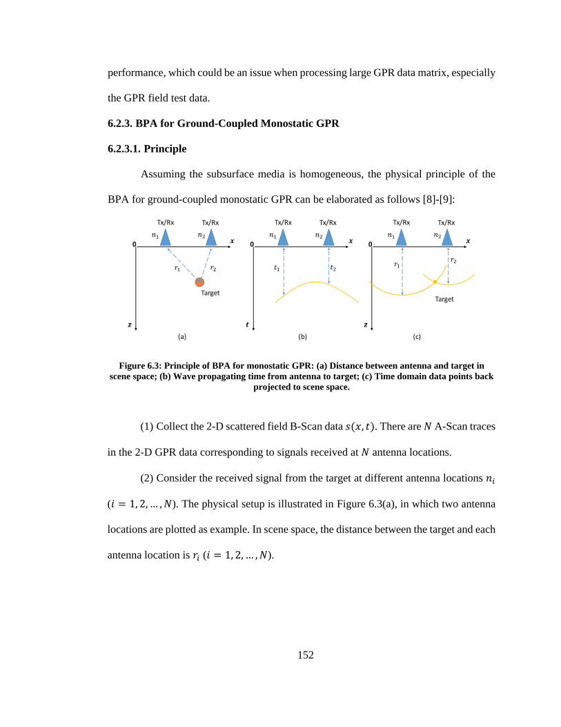
152

performance, which could be an issue when processing large GPR data matrix, especially

the GPR field test data.

6.2.3. BPA for Ground-Coupled Monostatic GPR

6.2.3.1. Principle

Assuming the subsurface media is homogeneous, the physical principle of the

BPA for ground-coupled monostatic GPR can be elaborated as follows [8]-[9]:

Figure 6.3: Principle of BPA for monostatic GPR: (a) Distance between antenna and target in

scene space; (b) Wave propagating time from antenna to target; (c) Time domain data points back

projected to scene space.

(1) Collect the 2-D scattered field B-Scan data 𝑠(𝑥, 𝑡). There are 𝑁 A-Scan traces

in the 2-D GPR data corresponding to signals received at 𝑁 antenna locations.

(2) Consider the received signal from the target at different antenna locations 𝑛𝑖

(𝑖 = 1, 2, … , 𝑁). The physical setup is illustrated in Figure 6.3(a), in which two antenna

locations are plotted as example. In scene space, the distance between the target and each

antenna location is 𝑟𝑖 (𝑖 = 1, 2, … , 𝑁).

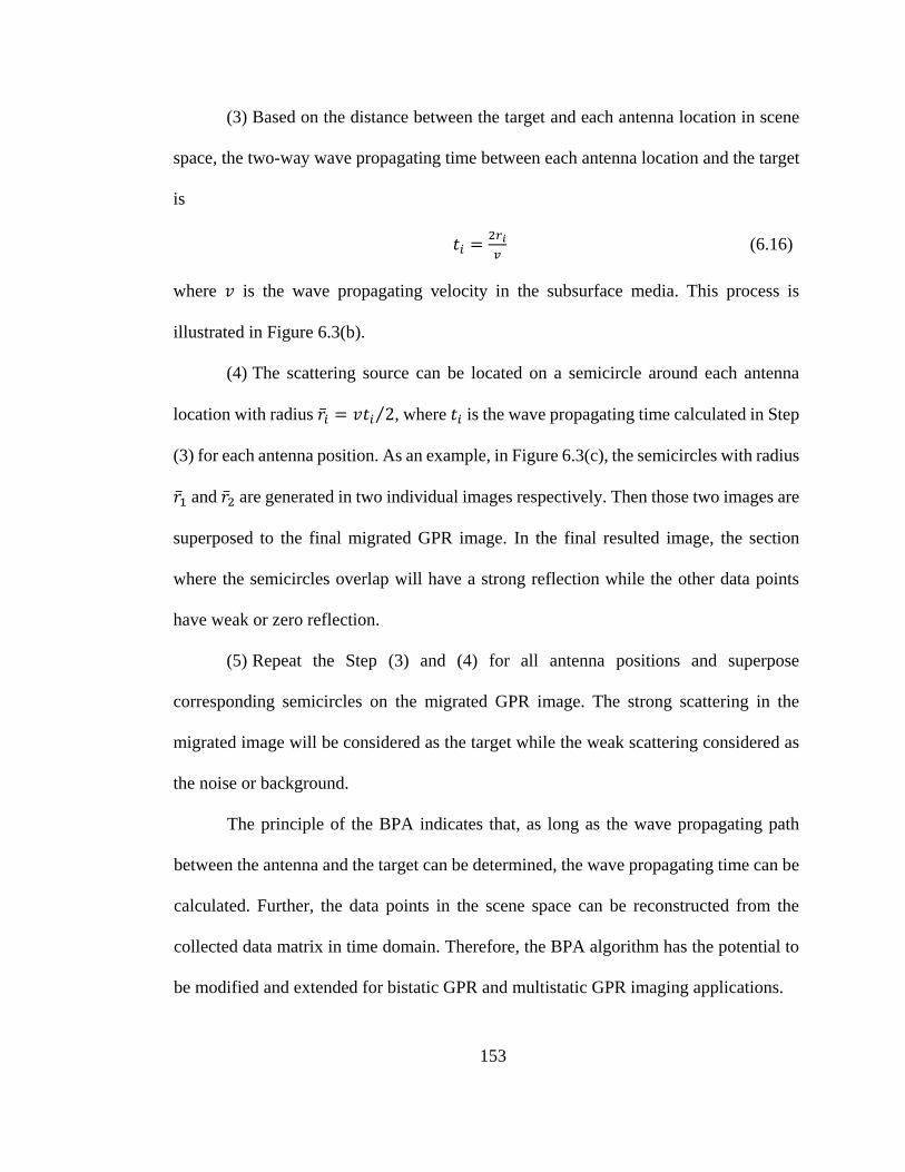
153

(3) Based on the distance between the target and each antenna location in scene

space, the two-way wave propagating time between each antenna location and the target

is

𝑡𝑖 =2𝑟𝑖

𝑣 (6.16)

where 𝑣 is the wave propagating velocity in the subsurface media. This process is

illustrated in Figure 6.3(b).

(4) The scattering source can be located on a semicircle around each antenna

location with radius �̅�𝑖 = 𝑣𝑡𝑖 2⁄ , where 𝑡𝑖 is the wave propagating time calculated in Step

(3) for each antenna position. As an example, in Figure 6.3(c), the semicircles with radius

�̅�1 and �̅�2 are generated in two individual images respectively. Then those two images are

superposed to the final migrated GPR image. In the final resulted image, the section

where the semicircles overlap will have a strong reflection while the other data points

have weak or zero reflection.

(5) Repeat the Step (3) and (4) for all antenna positions and superpose

corresponding semicircles on the migrated GPR image. The strong scattering in the

migrated image will be considered as the target while the weak scattering considered as

the noise or background.

The principle of the BPA indicates that, as long as the wave propagating path

between the antenna and the target can be determined, the wave propagating time can be

calculated. Further, the data points in the scene space can be reconstructed from the

collected data matrix in time domain. Therefore, the BPA algorithm has the potential to

be modified and extended for bistatic GPR and multistatic GPR imaging applications.

154


Figure 6.4: Implementation of BPA for ground-coupled monostatic GPR

The monostatic GPR configuration is plotted in Figure 6.4. The implementation

of the BPA for ground-coupled monostatic can be described as follows [10]-[11]:


in the 2-D GPR data corresponding to signals received at 𝑁 antenna locations. For the

𝑖th antenna location, the coordinate of the antenna is (𝑥𝑖 , 0).

(2) For a given scene point 𝑃(𝑥0, 𝑧0) in the GPR testing scenario, the GPR signal

transmits from the antenna, propagates to the scene point, and reflects back to the

antenna.

(3) For the 𝑖th antenna location, the round-trip distance between the antenna at

(𝑥𝑖 , 0) and the scene point 𝑃 at (𝑥0, 𝑧0) can be calculated as:

𝑑𝑃,𝑖 = 2√(𝑥0 − 𝑥𝑖)2 + 𝑧02 (6.17)

The two-way wave propagating time is

155

𝑡𝑃,𝑖 =𝑑𝑃,𝑖

𝑣=

2√(𝑥0−𝑥𝑖)2+𝑧02

𝑣=

2√(𝑥0−𝑥𝑖)2+𝑧02

𝑐 √𝜀𝑟⁄ (6.18)

where 𝜀𝑟 is the dielectric constant of the subsurface media. Here we assume that the

subsurface is a homogeneous media.

(4) For this given scene point 𝑃, calculate the two-way wave propagating time

from 𝑃 to each of the antenna position as {𝑡𝑃,1, 𝑡𝑃,2, … , 𝑡𝑃,𝑁}.

(5) The scattering signal of scene point 𝑃 is recorded in all the 𝑁 received signals

at the 𝑁 antenna locations. Denote the A-Scan trace signal at 𝑖th antenna is 𝑠𝑖(𝑡).

Interpolate in the 𝑠𝑖(𝑡) to obtain the scattering from point 𝑃 in the 𝑖th A-Scan trace:

𝑆𝑃,𝑖 = 𝑠𝑖(𝜏)|𝜏=𝑡𝑃,𝑖 (6.19)

(6) Perform interpolation and Eq. (6.19) on all the A-Scan traces, the scattering

from point 𝑃 in each A-Scan trace can be obtained as {𝑆𝑃,1, 𝑆𝑃,2, … , 𝑆𝑃,𝑁}. If point 𝑃 is

out of the illuminated area of the 𝑘th antenna location, then 𝑆𝑃,𝑘 is set to 0.

(7) The final value of the point 𝑃(𝑥0, 𝑧0) in the scene space can be formulated as:

𝑆𝑖𝑚𝑎𝑔𝑒(𝑥0, 𝑧0) = ∑ 𝑆𝑃,𝑖𝑁𝑖=1 (6.20)

(8) Repeat Step (2)-(7) for all the points in the scene space to produce the

migrated GPR image.

Considering the interpolation is the most time consuming computation in this

implementation, let us quantify how many interpolations are performed to complete this

migration process. For GPR data matrix or the imaging region of size 𝑀 × 𝑁, signals are

recorded at 𝑁 antenna locations as 𝑁 A-Scan traces, and each A-Scan trace consists of

𝑀 data points. Assume we set a scene space of size 𝑀0 × 𝑁0. In this implementation of

156

BPA, a point 𝑃 in the scene space is given and the scattering signal of this point in each

A-Scan trace is calculated by interpolation. Then the scattering signals recorded in each

A-Scan traces are projected back to the point 𝑃. So 𝑁 interpolations are required for one

data point in the scene space. This process will be repeated for all data points in the GPR

imaging scene space for 𝑀0𝑁0 times. Finally, 𝑀0𝑁0𝑁 times of interpolation are

computed during the BPA migration process.


An alternative implementation was proposed in Ref. [12] comprising less times

of interpolation:


in the 2-D GPR data corresponding to signals received at 𝑁 antenna locations. For the

𝑖th antenna location, the coordinate of the antenna is (𝑥𝑖 , 0). Initialize the migrated GPR

image as 𝑆𝑖𝑚𝑎𝑔𝑒(𝑥, 𝑧) consisting of 𝑀0 × 𝑁0 scene points. For a given scene point

𝑃(𝑥0, 𝑧0) in the GPR testing scenario, the GPR signal transmits from the antenna,

propagates to the scene point, and reflects back to the antenna.

(2) For the 𝑖th antenna location, the round-trip distance between the antenna at

(𝑥𝑖 , 0) and the scene point 𝑃 at (𝑥0, 𝑧0) can be calculated as:

𝑑𝑃,𝑖 = 2√(𝑥0 − 𝑥𝑖)2 + 𝑧02 (6.21)

The two-way wave propagating time is

𝑡𝑃,𝑖 =𝑑𝑃,𝑖

𝑣=

2√(𝑥0−𝑥𝑖)2+𝑧02

𝑣=

2√(𝑥0−𝑥𝑖)2+𝑧02

𝑐 √𝜀𝑟⁄ (6.22)

157

where 𝜀𝑟 is the dielectric constant of the subsurface media. Here we assume that the

subsurface is a homogeneous media.

(3) For the 𝑖th antenna location, calculate the two-way wave propagating time

from it to each of the scene points in the scene space 𝑆𝑖𝑚𝑎𝑔𝑒(𝑥, 𝑧) as a matrix:

𝑇𝑖 = [

𝑡𝑖(𝑥1, 𝑧1) ⋯ 𝑡𝑖(𝑥𝑁0, 𝑧1)

⋮ ⋱ ⋮𝑡𝑖(𝑥1, 𝑧𝑀0

) ⋯ 𝑡𝑖(𝑥𝑁0, 𝑧𝑀0

)] (6.23)

(4) The 𝑖th A-Scan trace at the 𝑖th antenna location records the scattering signal

from all the scene points in 𝑆𝑖𝑚𝑎𝑔𝑒(𝑥, 𝑧). Denote the A-Scan trace signal collected at 𝑖th

antenna location is 𝑠𝑖(𝑡). Interpolate in the 𝑠𝑖(𝑡) to obtain the scattering from point

𝑃(𝑥𝑛, 𝑧𝑚) that recorded in the 𝑖th A-Scan trace, and project this scattering back to the

scene space:

𝑆𝑖(𝑥𝑛, 𝑧𝑚) = 𝑠𝑖(𝜏)|𝜏=𝑡𝑖(𝑥𝑛,𝑧𝑚) (6.24)

Eq. (6.24) represents the contribution 𝑆𝑖(𝑥, 𝑧) of the 𝑖th A-Scan trace to the migrated

image in scene space. For those scene points out of the illuminated area of the 𝑖th antenna

location, their corresponding values in 𝑆𝑖(𝑥, 𝑧) are set to 0.

(5) Repeat Step (2)-(4) on all the A-Scan traces, the contribution of each A-Scan

trace to the migrated image can be obtained as {𝑆1(𝑥, 𝑧), 𝑆2(𝑥, 𝑧), … , 𝑆𝑁(𝑥, 𝑧)}. Finally,

the migrated image can be formulated as:

𝑆𝑖𝑚𝑎𝑔𝑒(𝑥, 𝑧) = ∑ 𝑆𝑖(𝑥, 𝑧)𝑁𝑖=1 (6.25)

In this implementation of BPA, an A-Scan trace received at the 𝑖th antenna

location is given and the scattering signals from all the scene points recorded in this A-

Scan trace are calculated by interpolation. Then the scattering signals from all the scene

158

points recorded in this A-Scan trace are projected back to the scene space. So just one

interpolation is applied when calculating the contribution of the 𝑖th A-Scan signal to the

scene space. This process will be repeated for all antenna locations by 𝑁 times. Totally,

only 𝑁 times of interpolation are computed during the BPA migration process.

6.2.3.4. Comparison between Two Implementations

Comparing to the implement in Sec. 6.2.3.2, the implementation in Sec. 6.2.3.3

has three advantages:

(1) Since much less times of interpolation are performed, this implementation of

BPA has much lower computational cost.

(2) The data in each A-Scan are only accessed within one single loop, so the

process or computation on each A-Scan signal is independent to each other, which

benefits the parallel processing and computing.

(3) The A-Scan is used as a unit in each loop within the implementation, so,

highly vectorized programming scheme can be utilized in MATLAB to implement the

algorithm with concise and efficient code.

Therefore, the implementation of BPA described in Sec. 6.2.3.3 is a better option

from multiple aspects. All the discussions on BPA in the following sections of this

chapter will be based on this implementation.

6.2.4. Comparison between SMA and BPA

Comparisons between the SMA and BPA for GPR imaging are summarized as

follows:

159

Image Quality: The range resolutions of the SMA and BPA are nearly the same

for experimental measurements [13]. On the other hand, the effects of the antenna’s finite

beam-width is incorporated in the BPA, since the back-projection is only performed on

the scene points that fall inside the antenna’s illuminated area. Thus, BPA performs better

than SMA when dealing with the antenna’s side-lobes.

Computational Cost: The time complexity of BPA is 𝒪(𝑁3). The time

complexity of conventional SMA for monostatic GPR imaging is only 𝒪(𝑁2), while for

bistatic GPR imaging, the improved SMA described in Sec. 6.2.2 also has time

complexity of 𝒪(𝑁3). Thus, for potential multistatic GPR imaging, the time complexity

of BPA and SMA are close to each other. However, BPA lends itself naturally to parallel

processing [12]. Firstly, BPA can be performed on any selected sub-region of the scene

space, so the scene space can be divided into several sub-region and each sub-region can

be imaged separately on different hardware processors. Secondly, the BPA processes

each A-Scan signal individually, so the GPR data matrix can be divided into several

groups of A-Scan traces and each group can be processed parallel on separated

processors. Thus, BPA is suitable for parallel computation. Overall speaking, the

computational cost of BPA is not a severe issue for multistatic GPR imaging.

Real-Time Application: For some GPR applications, especially multistatic GPR

applications such as landmine detection [15]-[17], the real-time GPR imaging is urgently

demanded. Since the BPA processes each A-Scan signal individually, so it can generate

the GPR image as collecting the data. While for the SMA, all the measurements have to

be record as a B-Scan since cross range FFT is one of the steps in SMA, so SMA has to

160

wait until the whole GPR inspection is completed. Therefore, the BPA is more suitable

for real-time GPR imaging than SMA.

Geometry Configuration: Due to the FFT operation, SMA requires a uniform

spatial sampling along the cross range direction, which limits its geometry configuration.

This could be an issue for multistatic GPR. The increments in the separation distances

between different transmitter antennas and receiver antennas may not be uniform, so the

overall spatial distribution of the GPR measurements from all bistatic pairs is not uniform

for the data fusion process. Therefore, the geometry configuration requirement of SMA

limits its utilization in multistatic GPR application. While for the BPA, as long as the

coordinates of bistatic pairs are known, the data points can be accurately projected back

to the scene space.

In summary, BPA is more suitable for multistatic GPR imaging than SMA from

above four perspectives. A BPA imaging algorithm would be developed in this chapter

for multistatic GPR imaging application in the following sections.

6.3. Ground-Coupled Multistatic GPR Imaging Methodology

As a starting point, back-projection imaging algorithm for ground-coupled

multistatic GPR is described in this section. It is a special and simplified case of air-

coupled multistatic imaging algorithm.

6.3.1. System Configuration

Given a multistatic GPR system with 𝑀 transmitter antennas and 𝑁 receiver

antennas depicted as Figure 6.5, there are totally 𝑀 × 𝑁 bistatic pairs or transceiver

antennas pairs. The antennas are assembled on an antenna platform. During the GPR

161

survey, the antenna platform moves along the cross-range direction and records signals

at 𝐾 positions. At each data collection location, all transmitter antennas are switched on

sequentially. When one transmitter antenna is on, 𝑁 A-Scan traces are recorded by 𝑁

receiver antennas respectively and simultaneously. After switching between all 𝑀

transmitter antennas, totally 𝑀 × 𝑁 A-Scan traces are recorded by the GPR system. This

data acquisition step is repeat at every antenna platform scanning position. Finally, 𝑀 ×

𝑁 × 𝐾 A-Scan traces are recorded and assembled into one GPR data matrix for this GPR

inspection job.

Figure 6.5: Ground-coupled multistatic GPR configuration.

6.3.2. BPA for Ground-Coupled Multistatic GPR Imaging

The back-projection based multistatic GPR imaging algorithm aims to fuse the

𝑀 × 𝑁 × 𝐾 A-Scan traces from different bistatic pairs and signal measurement locations

into one B-Scan image. The imaging configuration of ground-coupled multistatic GPR

is illustrated in Figure 6.6. A 2-D coordinate in scene space is constructed and all the

bistatic pairs share the same coordinate system. The x-axis is the cross-range direction or

the GPR scanning direction. Antenna platform consisting of 𝑀 transmitter antennas and

162

𝑁 receiver antennas is moving along the x-axis during the GPR survey. The z-axis is the

range direction or the penetrating depth. Assume the subsurface media is a homogenous

media of dielectric constant 𝜀𝑟.

Figure 6.6: Ground-coupled multistatic GPR imaging.

As an example, one bistatic pair at one antenna platform scanning location is

plotted in Figure 6.6. When the antenna platform is at the 𝑘th scanning location (𝑘 =

1, 2, … , 𝐾), the coordinate of the 𝑖th transmitter antenna (𝑖 = 1, 2, … , 𝑀) is (𝑥𝑖,𝑘, 0) and

the coordinate of the 𝑗th receiver antenna (𝑗 = 1, 2, … , 𝑁) is (𝑥𝑗,𝑘, 0). In this example, the

𝑖th transmitter antenna and the 𝑗th receiver antenna form a bistatic pair (𝑖, 𝑗), and the

spatial offset between them is 𝑑𝑖,𝑗 which is a fixed value during the GPR survey.

Define the scene region as 𝑆 ∈ ℝ𝑀0×𝑁0 consisting of 𝑀0 × 𝑁0 scene points. For

a scene point 𝑃(𝑥𝑚, 𝑧𝑛) where 𝑚 = 1, 2, … , 𝑀0 and 𝑁 = 1, 2, … , 𝑁0, the GPR signal

transmits from the 𝑖th transmitter antenna to it and then reflects back to the 𝑗th receiver

163

antenna at the 𝑘th scanning position. The wave propagating distance between the 𝑖th

transmitter antenna at (𝑥𝑖,𝑘, 0) and the scene point 𝑃 at (𝑥𝑚, 𝑧𝑛) can be calculated as:

𝑑𝑖,𝑘(𝑥𝑚, 𝑧𝑛) = √(𝑥𝑚 − 𝑥𝑖,𝑘)2 + 𝑧𝑛2 (6.26)

The corresponding wave propagating time for 𝑑𝑖,𝑘(𝑥𝑚, 𝑧𝑛) is:

𝑡𝑖,𝑘(𝑥𝑚, 𝑧𝑛) =𝑑𝑖,𝑘(𝑥𝑚,𝑧𝑛)

𝑣=

√(𝑥𝑚−𝑥𝑖,𝑘)2+𝑧𝑛2

𝑣=

√(𝑥𝑚−𝑥𝑖,𝑘)2+𝑧𝑛2

𝑐 √𝜀𝑟⁄ (6.27)

Similarly, the wave propagating distance from the scene point 𝑃 at (𝑥𝑚, 𝑧𝑛) to the 𝑗th

receiver antenna at (𝑥𝑗,𝑘, 0) and corresponding propagating time can be formulated as:

𝑑𝑗,𝑘(𝑥𝑚, 𝑧𝑛) = √(𝑥𝑚 − 𝑥𝑗,𝑘)2 + 𝑧𝑛2 (6.28)

𝑡𝑗,𝑘(𝑥𝑚, 𝑧𝑛) =𝑑𝑗,𝑘(𝑥𝑚,𝑧𝑛)

𝑣=

√(𝑥𝑚−𝑥𝑗,𝑘)2+𝑧𝑛2

𝑣=


𝑐 √𝜀𝑟⁄ (6.29)

Adding Eq. (6.27) and Eq. (6.29) together, the round-trip wave propagating time between

the scene point 𝑃(𝑥𝑚, 𝑧𝑛) and the bistatic pair (𝑖, 𝑗) is expressed as:

𝑡(𝑖,𝑗),𝑘(𝑥𝑚, 𝑧𝑛) = 𝑡𝑖,𝑘(𝑥𝑚, 𝑧𝑛) + 𝑡𝑗,𝑘(𝑥𝑚, 𝑧𝑛)

=√(𝑥𝑚−𝑥𝑖,𝑘)2+𝑧𝑛

2

𝑐 √𝜀𝑟⁄+


𝑐 √𝜀𝑟⁄ (6.30)

For the bistatic pair (𝑖, 𝑗), calculate the two-way wave propagating times between

it and each of the scene points in the scene space 𝑆 as a matrix:

𝑇(𝑖,𝑗),𝑘(𝑥, 𝑧) = [

𝑡(𝑖,𝑗),𝑘(𝑥1, 𝑧1) ⋯ 𝑡(𝑖,𝑗),𝑘(𝑥1, 𝑧𝑁0)

⋮ ⋱ ⋮𝑡(𝑖,𝑗),𝑘(𝑥𝑀0

, 𝑧1) ⋯ 𝑡(𝑖,𝑗),𝑘(𝑥𝑀0, 𝑧𝑁0

)] (6.31)

The A-Scan trace measured by bistatic pair (𝑖, 𝑗) at the 𝑘th antenna platform

location 𝑠(𝑖,𝑗),𝑘(𝑡) records the scattering signal from all the scene points in 𝑆𝑖𝑚𝑎𝑔𝑒(𝑥, 𝑧).

164

Interpolate in the 𝑠(𝑖,𝑗),𝑘(𝑡) to obtain the scattering from point 𝑃(𝑥𝑛, 𝑧𝑚) that recorded

by the bistatic pair (𝑖, 𝑗) at the 𝑘th antenna platform location, and project this scattering

back to the scene space:

𝑆(𝑖,𝑗),𝑘(𝑥𝑛, 𝑧𝑚) = 𝑠(𝑖,𝑗),𝑘(𝜏)|𝜏=𝑡(𝑖,𝑗),𝑘(𝑥𝑛,𝑧𝑚) (6.32)

The contribution 𝑆(𝑖,𝑗),𝑘(𝑥, 𝑧) of the bistatic pair (𝑖, 𝑗) at 𝑘th antenna platform location to

the migrated image in scene space can be formulated as:

𝑆(𝑖,𝑗),𝑘(𝑥, 𝑧) = [

𝑆(𝑖,𝑗),𝑘(𝑥1, 𝑧1) ⋯ 𝑆(𝑖,𝑗),𝑘(𝑥1, 𝑧𝑁0)

⋮ ⋱ ⋮𝑆(𝑖,𝑗),𝑘(𝑥𝑀0

, 𝑧1) ⋯ 𝑆(𝑖,𝑗),𝑘(𝑥𝑀0, 𝑧𝑁0

)] (6.33)

For those scene points out of the illuminated area of the bistatic pair (𝑖, 𝑗) at the 𝑘th

location, their corresponding values in 𝑆(𝑖,𝑗),𝑘(𝑥, 𝑧) are set to 0.

Repeating above processing for the bistatic pair (𝑖, 𝑗) on the A-Scan traces at

every platform location, the contribution of A-Scan traces at each antenna platform

location to the migrated image can be obtained as

{𝑆(𝑖,𝑗),1(𝑥, 𝑧), 𝑆(𝑖,𝑗),2(𝑥, 𝑧), … , 𝑆(𝑖,𝑗),𝐾(𝑥, 𝑧)}. The imaging data matrix produced by the

static pair (𝑖, 𝑗) can be formulated as:

𝑆(𝑖,𝑗)(𝑥, 𝑧) = ∑ 𝑆(𝑖,𝑗),𝑘(𝑥, 𝑧)𝐾𝑘=1 (6.34)

Repeating above processing for every bistatic pair in the multistatic GPR system,

the imaging data matrix for each bistatic pair can be obtained as 𝑆(𝑖,𝑗)(𝑥, 𝑧) where 𝑖 =

1, 2, … , 𝑀 and 𝑗 = 1, 2, … , 𝑁. The final migrated GPR image can be formulated as the

superposition of the 𝑆(𝑖,𝑗)(𝑥, 𝑧) from each bistatic pair:

𝑆image(𝑥, 𝑧) = ∑ ∑ 𝑆(𝑖,𝑗)(𝑥, 𝑧)𝑁𝑗=1

𝑀𝑖=1 (6.35)

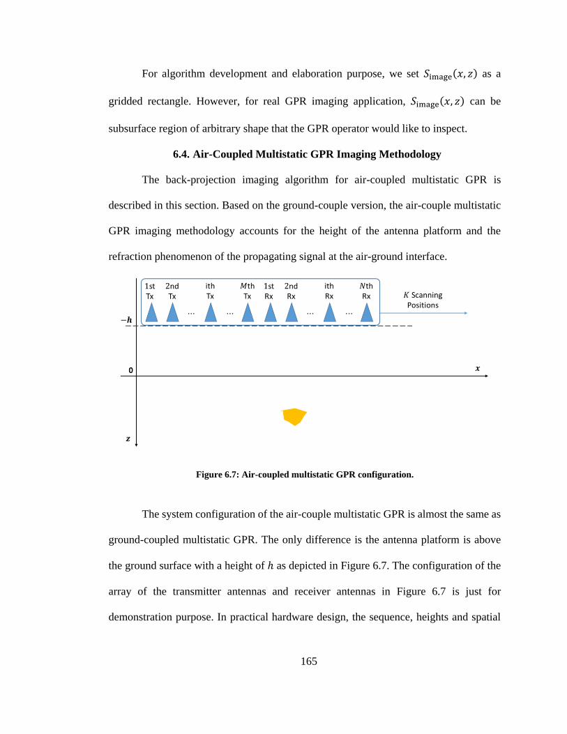
165

For algorithm development and elaboration purpose, we set 𝑆image(𝑥, 𝑧) as a

gridded rectangle. However, for real GPR imaging application, 𝑆image(𝑥, 𝑧) can be

subsurface region of arbitrary shape that the GPR operator would like to inspect.

6.4. Air-Coupled Multistatic GPR Imaging Methodology

The back-projection imaging algorithm for air-coupled multistatic GPR is

described in this section. Based on the ground-couple version, the air-couple multistatic

GPR imaging methodology accounts for the height of the antenna platform and the

refraction phenomenon of the propagating signal at the air-ground interface.

Figure 6.7: Air-coupled multistatic GPR configuration.

The system configuration of the air-couple multistatic GPR is almost the same as

ground-coupled multistatic GPR. The only difference is the antenna platform is above

the ground surface with a height of ℎ as depicted in Figure 6.7. The configuration of the

array of the transmitter antennas and receiver antennas in Figure 6.7 is just for

demonstration purpose. In practical hardware design, the sequence, heights and spatial

166

offsets of the antennas can be adjusted to achieve different system specifications [18]-

[21].

Figure 6.8: Air-coupled multistatic GPR imaging.

One bistatic pair at one antenna platform scanning location is plotted in Figure

6.8. When the antenna platform is at the 𝑘th scanning location (𝑘 = 1, 2, … , 𝐾), the

coordinate of the 𝑖th transmitter antenna (𝑖 = 1, 2, … , 𝑀) is (𝑥𝑖,𝑘, −ℎ) and the coordinate

of the 𝑗th receiver antenna (𝑗 = 1, 2, … , 𝑁) is (𝑥𝑗,𝑘, −ℎ). In this example, the 𝑖th

transmitter antenna and the 𝑗th receiver antenna form a bistatic pair (𝑖, 𝑗), and the spatial

offset between them is 𝑑𝑖,𝑗 which is a fixed value during the GPR survey.

Define the scene region as 𝑆 ∈ ℝ𝑀0×𝑁0 consisting of 𝑀0 × 𝑁0 scene points. For

a scene point 𝑃(𝑥𝑚, 𝑧𝑛) where 𝑚 = 1, 2, … , 𝑀0 and 𝑁 = 1, 2, … , 𝑁0, the GPR signal

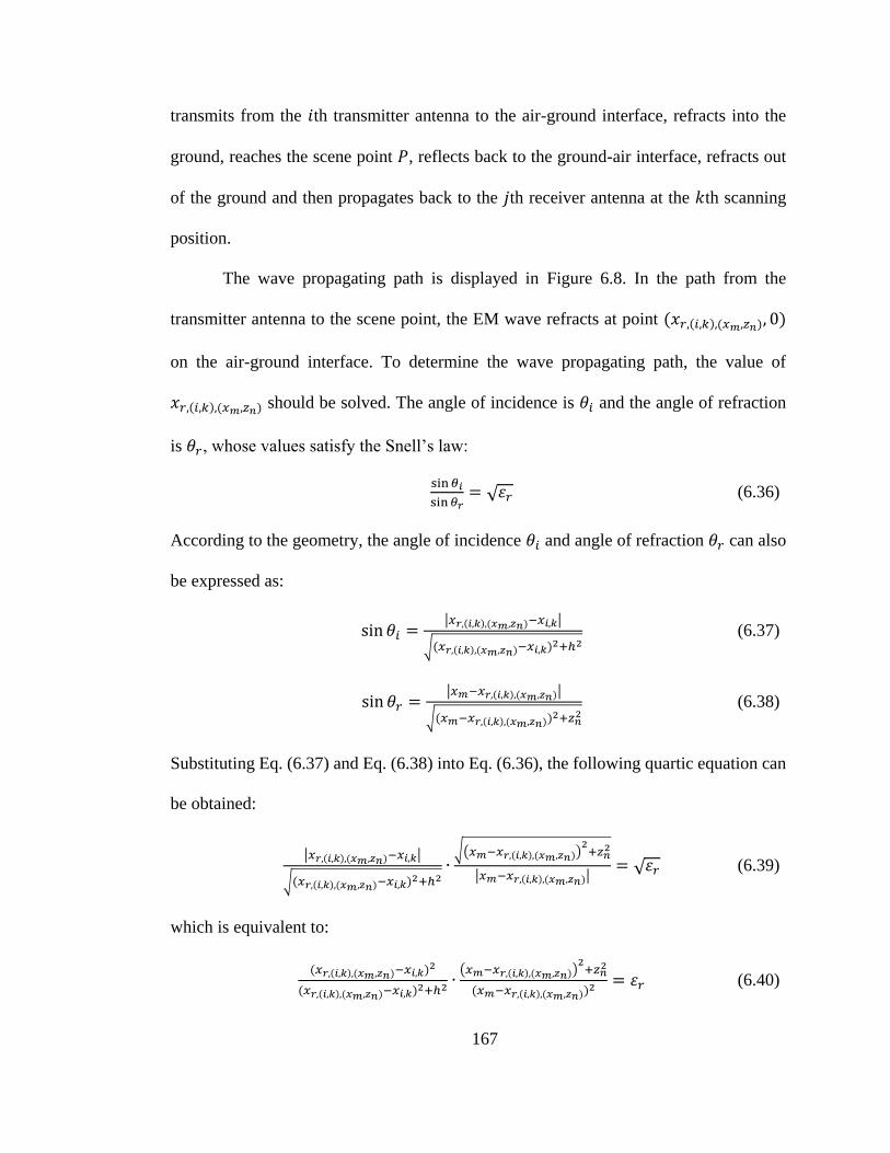
167

transmits from the 𝑖th transmitter antenna to the air-ground interface, refracts into the

ground, reaches the scene point 𝑃, reflects back to the ground-air interface, refracts out

of the ground and then propagates back to the 𝑗th receiver antenna at the 𝑘th scanning

position.

The wave propagating path is displayed in Figure 6.8. In the path from the

transmitter antenna to the scene point, the EM wave refracts at point (𝑥𝑟,(𝑖,𝑘),(𝑥𝑚,𝑧𝑛), 0)

on the air-ground interface. To determine the wave propagating path, the value of

𝑥𝑟,(𝑖,𝑘),(𝑥𝑚,𝑧𝑛) should be solved. The angle of incidence is 𝜃𝑖 and the angle of refraction

is 𝜃𝑟, whose values satisfy the Snell’s law:

sin 𝜃𝑖

sin 𝜃𝑟= √𝜀𝑟 (6.36)

According to the geometry, the angle of incidence 𝜃𝑖 and angle of refraction 𝜃𝑟 can also

be expressed as:

sin 𝜃𝑖 =|𝑥𝑟,(𝑖,𝑘),(𝑥𝑚,𝑧𝑛)−𝑥𝑖,𝑘|

√(𝑥𝑟,(𝑖,𝑘),(𝑥𝑚,𝑧𝑛)−𝑥𝑖,𝑘)2+ℎ2 (6.37)

sin 𝜃𝑟 =|𝑥𝑚−𝑥𝑟,(𝑖,𝑘),(𝑥𝑚,𝑧𝑛)|

√(𝑥𝑚−𝑥𝑟,(𝑖,𝑘),(𝑥𝑚,𝑧𝑛))2+𝑧𝑛2 (6.38)

Substituting Eq. (6.37) and Eq. (6.38) into Eq. (6.36), the following quartic equation can

be obtained:

|𝑥𝑟,(𝑖,𝑘),(𝑥𝑚,𝑧𝑛)−𝑥𝑖,𝑘|

√(𝑥𝑟,(𝑖,𝑘),(𝑥𝑚,𝑧𝑛)−𝑥𝑖,𝑘)2+ℎ2∙

√(𝑥𝑚−𝑥𝑟,(𝑖,𝑘),(𝑥𝑚,𝑧𝑛))2

+𝑧𝑛2

|𝑥𝑚−𝑥𝑟,(𝑖,𝑘),(𝑥𝑚,𝑧𝑛)|= √𝜀𝑟 (6.39)

which is equivalent to:

(𝑥𝑟,(𝑖,𝑘),(𝑥𝑚,𝑧𝑛)−𝑥𝑖,𝑘)2

(𝑥𝑟,(𝑖,𝑘),(𝑥𝑚,𝑧𝑛)−𝑥𝑖,𝑘)2+ℎ2 ∙(𝑥𝑚−𝑥𝑟,(𝑖,𝑘),(𝑥𝑚,𝑧𝑛))

2+𝑧𝑛

2

(𝑥𝑚−𝑥𝑟,(𝑖,𝑘),(𝑥𝑚,𝑧𝑛))2 = 𝜀𝑟 (6.40)

168

𝑥𝑟,(𝑖,𝑘),(𝑥𝑚,𝑧𝑛) can be solved from Eq. (6.40). Solving a quartic equation is a time

consuming computation. Considering there are 𝑀 × 𝑁 bistatic pairs in the system and 𝐾

antenna platform scanning positions, for a single scene point, the quartic equation in Eq.

(6.40) will be solved for 𝑀 × 𝑁 × 𝐾 times. To alleviate the computational cost, the

approximate value of 𝑥𝑟,(𝑖,𝑘),(𝑥𝑚,𝑧𝑛) will be applied in this multistatic GPR imaging

method instead of solving the quartic equation (6.40).

Denote the intersection point of the x-axis and the direct line from the antenna

(𝑥𝑖,𝑘, −ℎ) to the scene point (𝑥𝑚, 𝑧𝑛) is (𝑥𝑐,(𝑖,𝑘),(𝑥𝑚,𝑧𝑛), 0). According to geometry of the

setup, the following relation on (𝑥𝑖,𝑘, −ℎ), (𝑥𝑐,(𝑖,𝑘),(𝑥𝑚,𝑧𝑛), 0) and (𝑥𝑚, 𝑧𝑛) can be

formulated:

𝑥𝑐,(𝑖,𝑘),(𝑥𝑚,𝑧𝑛)−𝑥𝑖,𝑘

𝑥𝑚−𝑥𝑐,(𝑖,𝑘),(𝑥𝑚,𝑧𝑛)=

ℎ

𝑧𝑛 (6.41)

Thus, the value of 𝑥𝑐,(𝑖,𝑘),(𝑥𝑚,𝑧𝑛) can be calculated by

𝑥𝑐,(𝑖,𝑘),(𝑥𝑚,𝑧𝑛) =𝑧𝑛𝑥𝑖,𝑘+ℎ𝑥0

𝑧𝑛+ℎ (6.42)

Once 𝑥𝑐,(𝑖,𝑘),(𝑥𝑚,𝑧𝑛) is known, according to the derivation in Ref. [22]-[23], the

approximation of 𝑥𝑟,(𝑖,𝑘),(𝑥𝑚,𝑧𝑛) can be formulated as:

𝑥𝑟,(𝑖,𝑘),(𝑥𝑚,𝑧𝑛) =

{

𝑥𝑚 + (𝑥𝑐,(𝑖,𝑘),(𝑥𝑚,𝑧𝑛) − 𝑥𝑚) √𝜀𝑟⁄ ,

𝑥𝑚 + 𝑧𝑛 √𝜀𝑟 − 1⁄ ,

𝑥𝑚 − 𝑧𝑛 √𝜀𝑟 − 1⁄ ,

|𝑥𝑖,𝑘 − 𝑥𝑚| < (𝑧𝑛 + ℎ)√𝜀𝑟 (𝜀𝑟 − 1)⁄

𝑥𝑖,𝑘 − 𝑥𝑚 ≥ (𝑧𝑛 + ℎ)√𝜀𝑟 (𝜀𝑟 − 1)⁄

𝑥𝑖,𝑘 − 𝑥𝑚 ≤ −(𝑧𝑛 + ℎ)√𝜀𝑟 (𝜀𝑟 − 1)⁄

(6.43)

169

Once 𝑥𝑟 is solved, the wave path from the 𝑖th transmitter antenna at (𝑥𝑖,𝑘, 0) to

the scene point 𝑃 at (𝑥𝑚, 𝑧𝑛) when the antenna platform is at the 𝑘th location can be

determined. The wave propagating time on this path can be calculate as:

𝑡𝑖,𝑘(𝑥𝑚, 𝑧𝑛) =√(𝑥𝑟,(𝑖,𝑘),(𝑥𝑚,𝑧𝑛)−𝑥𝑖,𝑘)

2+ℎ2

𝑐+

√(𝑥𝑚−𝑥𝑟,(𝑖,𝑘),(𝑥𝑚,𝑧𝑛))2

+𝑧𝑛2

𝑐 √𝜀𝑟⁄ (6.44)

Similarly, when antenna platform is at the 𝑘th location, for the wave propagating

path from the scene point 𝑃 at (𝑥𝑚, 𝑧𝑛) to the 𝑗th receiver antenna at (𝑥𝑗,𝑘, 0), the

intersection point (𝑥𝑐,(𝑗,𝑘),(𝑥𝑚,𝑧𝑛), 0) and the refraction point (𝑥𝑟,(𝑗,𝑘),(𝑥𝑚,𝑧𝑛), 0) can be

determined as:

𝑥𝑐,(𝑗,𝑘),(𝑥𝑚,𝑧𝑛) =𝑧𝑛𝑥𝑗,𝑘+ℎ𝑥0

𝑧𝑛+ℎ (6.45)

𝑥𝑟,(𝑗,𝑘),(𝑥𝑚,𝑧𝑛) =

{

𝑥𝑚 + (𝑥𝑐,(𝑗,𝑘),(𝑥𝑚,𝑧𝑛) − 𝑥𝑚) √𝜀𝑟⁄ ,

𝑥𝑚 + 𝑧𝑛 √𝜀𝑟 − 1⁄ ,

𝑥𝑚 − 𝑧𝑛 √𝜀𝑟 − 1⁄ ,

|𝑥𝑗,𝑘 − 𝑥𝑚| < (𝑧𝑛 + ℎ)√𝜀𝑟 (𝜀𝑟 − 1)⁄

𝑥𝑗,𝑘 − 𝑥𝑚 ≥ (𝑧𝑛 + ℎ)√𝜀𝑟 (𝜀𝑟 − 1)⁄

𝑥𝑗,𝑘 − 𝑥𝑚 ≤ −(𝑧𝑛 + ℎ)√𝜀𝑟 (𝜀𝑟 − 1)⁄

(6.46)

Once the refraction point (𝑥𝑟,(𝑗,𝑘),(𝑥𝑚,𝑧𝑛), 0) is obtained, the wave propagating time on

this path can be calculate as

𝑡𝑗,𝑘(𝑥𝑚, 𝑧𝑛) =√(𝑥𝑟,(𝑗,𝑘),(𝑥𝑚,𝑧𝑛)−𝑥𝑗,𝑘)

2+ℎ2

𝑐+

√(𝑥𝑚−𝑥𝑟,(𝑗,𝑘),(𝑥𝑚,𝑧𝑛))2

+𝑧𝑛2

𝑐 √𝜀𝑟⁄ (6.47)

Adding Eq. (6.44) and Eq. (6.47) together, the round-trip wave propagating time between

the scene point 𝑃(𝑥𝑚, 𝑧𝑛) and the bistatic pair (𝑖, 𝑗) is expressed as:

𝑡(𝑖,𝑗),𝑘(𝑥𝑚, 𝑧𝑛) = 𝑡𝑖,𝑘(𝑥𝑚, 𝑧𝑛) + 𝑡𝑗,𝑘(𝑥𝑚, 𝑧𝑛)

=√(𝑥𝑟,(𝑖,𝑘),(𝑥𝑚,𝑧𝑛)−𝑥𝑖,𝑘)

2+ℎ2+√(𝑥𝑟,(𝑗,𝑘),(𝑥𝑚,𝑧𝑛)−𝑥𝑗,𝑘)

2+ℎ2

𝑐

170

+√(𝑥𝑚−𝑥𝑟,(𝑖,𝑘),(𝑥𝑚,𝑧𝑛))

2+𝑧𝑛

2+√(𝑥𝑚−𝑥𝑟,(𝑗,𝑘),(𝑥𝑚,𝑧𝑛))2

+𝑧𝑛2

𝑐 √𝜀𝑟⁄ (6.48)

For the bistatic pair (𝑖, 𝑗), calculate the two-way wave propagating times between

it and each of the scene points in the scene space 𝑆 as a matrix:

𝑇(𝑖,𝑗),𝑘(𝑥, 𝑧) = [

𝑡(𝑖,𝑗),𝑘(𝑥1, 𝑧1) ⋯ 𝑡(𝑖,𝑗),𝑘(𝑥1, 𝑧𝑁0)

⋮ ⋱ ⋮𝑡(𝑖,𝑗),𝑘(𝑥𝑀0

, 𝑧1) ⋯ 𝑡(𝑖,𝑗),𝑘(𝑥𝑀0, 𝑧𝑁0

)] (6.49)

The A-Scan trace measured by bistatic pair (𝑖, 𝑗) at the 𝑘th antenna platform

location 𝑠(𝑖,𝑗),𝑘(𝑡) records the scattering signal from all the scene points in 𝑆𝑖𝑚𝑎𝑔𝑒(𝑥, 𝑧).

Interpolate in the 𝑠(𝑖,𝑗),𝑘(𝑡) to obtain the scattering from point 𝑃(𝑥𝑛, 𝑧𝑚) that recorded

by the bistatic pair (𝑖, 𝑗) at the 𝑘th antenna platform location, and project this scattering

back to the scene space:

𝑆(𝑖,𝑗),𝑘(𝑥𝑛, 𝑧𝑚) = 𝑠(𝑖,𝑗),𝑘(𝜏)|𝜏=𝑡(𝑖,𝑗),𝑘(𝑥𝑛,𝑧𝑚) (6.50)

The contribution 𝑆(𝑖,𝑗),𝑘(𝑥, 𝑧) of the bistatic pair (𝑖, 𝑗) at 𝑘th antenna platform location to

the migrated image in scene space can be formulated as:

𝑆(𝑖,𝑗),𝑘(𝑥, 𝑧) = [

𝑆(𝑖,𝑗),𝑘(𝑥1, 𝑧1) ⋯ 𝑆(𝑖,𝑗),𝑘(𝑥1, 𝑧𝑁0)

⋮ ⋱ ⋮𝑆(𝑖,𝑗),𝑘(𝑥𝑀0

, 𝑧1) ⋯ 𝑆(𝑖,𝑗),𝑘(𝑥𝑀0, 𝑧𝑁0

)] (6.51)

For those scene points out of the illuminated area of the bistatic pair (𝑖, 𝑗) at the 𝑘th

location, their corresponding values in 𝑆(𝑖,𝑗),𝑘(𝑥, 𝑧) are set to 0.

Repeating above processing for the bistatic pair (𝑖, 𝑗) on the A-Scan traces at all

𝐾 platform locations, the contribution of A-Scan traces at each antenna platform location

to the migrated image can be obtained as {𝑆(𝑖,𝑗),1(𝑥, 𝑧), 𝑆(𝑖,𝑗),2(𝑥, 𝑧), … , 𝑆(𝑖,𝑗),𝐾(𝑥, 𝑧)}. The

imaging data matrix produced by the static pair (𝑖, 𝑗) can be formulated as:

171

𝑆(𝑖,𝑗)(𝑥, 𝑧) = ∑ 𝑆(𝑖,𝑗),𝑘(𝑥, 𝑧)𝐾𝑘=1 (6.52)

Repeating above processing for every bistatic pair in the multistatic GPR system,

the imaging data matrix for each bistatic pair can be obtained as 𝑆(𝑖,𝑗)(𝑥, 𝑧) where 𝑖 =

1, 2, … , 𝑀 and 𝑗 = 1, 2, … , 𝑁. The final migrated GPR image can be formulated as the

superposition of the 𝑆(𝑖,𝑗)(𝑥, 𝑧) from each bistatic pair:

𝑆image(𝑥, 𝑧) = ∑ ∑ 𝑆(𝑖,𝑗)(𝑥, 𝑧)𝑁𝑗=1

𝑀𝑖=1 (6.53)

The difference of this air-coupled multistatic GPR imaging method and the

ground-coupled version is the way to calculate the wave propagating time between the

scene point and the antennas.

6.5. Experimental Results

To evaluate the back-projection based multistatic GPR imaging method,

experiments are conducted with four sets of test data that are synthesized with the GPR

simulation tool GprMax [24]. In the first and second test cases, a ground-coupled

multistatic GPR is simulated. An air-coupled multistatic GPR is simulated in the third

and fourth test cases.

6.5.1. Ground-Coupled GPR Imaging Experiments

In this section, two sets of simulation data are created using GprMax program. In

our simulation, the GPR waveform is generated as a Ricker waveform (i.e. negative

normalized second derivative of a Gaussian pulse) with its center frequency being 2 GHz.

The multistatic configuration consists of one transmitter antenna and six receiver

antennas. Spatial offsets between the transmitter antenna and six receiver antennas are 5

cm, 10 cm, 20 cm, 30 cm, 40 cm and 50 cm respectively. The antenna platform is close

172

to the ground surface simulating the ground-coupled configuration. The antenna platform

moves uniformly from left to right along the horizontal direction and records the received

signal at 100 positions. The distance interval between two adjacent platform locations is

2 cm.

6.5.1.1. Simulation Data 1: Three Targets

In the first simulation setup, the subsurface media is modeled as a homogeneous

layer whose dielectric constant is 6.0. As depicted in Figure 6.9, three targets are buried

underground whose dielectric constants are all set to 8.0. The purpose of this test case is

to evaluate the effectiveness of the proposal multistatic GPR imaging method on targets

of various shapes. The dimensional specifications of the targets are listed as follows:

Pipe (cylinder object) – depth: 7.5 cm; diameter: 2.5 cm.

Man-made shape object – depth of top surface: 10 cm; depth of bottom surface: 20

cm; width of top part: 10 cm; width of bottom part: 20 cm; thickness of top part: 5

cm; thickness of bottom part: 5 cm.

Plate – depth: 8.5 cm; width: 15 cm; thickness: 0.5 cm.

Figure 6.9: Ground-coupled multistatic GPR testing setup – three buried targets.

173

The multistatic system in this simulation consists of one transmitter antenna and

six receiver antennas, so six GPR data matrices are produced by six bistatic pairs. The

raw B-Scan images produced by the Tx1-Rx1 pair and Tx1-Rx5 pair are plotted as Figure

6.10(a) and (b) respectively.

(a)

(b)

Figure 6.10: Ground-coupled multistatic GPR raw B-Scan – three buried targets: (1) Tx1-Rx1

pair; (2) Tx1-Rx5 pair.

If each bistatic pair is regarded as an individual GPR system, the migrated B-Scan

images generated by the proposed algorithm are displayed in Figure 6.11(a) and (b) for

pair Tx1-Rx1 and Tx1-Rx5 respectively. As shown in Figure 6.11(a), for the B-Scan

produced by bistatic pair Tx1-Rx1, the resolution of the targets is good, nevertheless, the

174

bottom of the man-made shape target can’t be detected and the SCR is low. As depicted

in Figure 6.11(b), for the B-Scan image obtained from bistatic pair Tx1-Rx5, the bottom

of the middle target can be reconstructed accurately and the SCR is high, however, the

resolution is not good comparing to bistatic pair Tx1-Rx1. Because of the variety of

spatial offsets in different bistatic antenna pairs, the characteristics of both the target and

clutter vary.

(a)

(b)

Figure 6.11: Ground-coupled multistatic GPR migrated B-Scan – three buried targets: (1) Tx1-

Rx1 pair; (2) Tx1-Rx5 pair.

Now considering all six bistatic pairs as a multistatic system, the GPR data matrix

is processed by the proposed multistatic GPR imaging method, and the resulted GPR

175

image is plotted as Figure 6.12. The imaging result is consistent with the geometry setup

depicted in Figure 6.9. It combines the advantages of all bistatic pairs, in which, the

resolution is good and the shapes of the targets are reconstructed accurately. Moreover,

this migrated GPR image testifies to the discussion in Sec. 6.1 that the radar imaging

specifications, such as SNR and SCR, benefit from the multistatic configuration because

of information gained from various antenna pairs and multiple radar cross sections.

Figure 6.12: Ground-coupled multistatic GPR migrated B-Scan using proposed multistatic

imaging method – three buried targets

6.5.1.2. Simulation Data 2: Congested Pipes

In the second simulation setup for ground-coupled multistatic GPR inspection,

the subsurface media is also modeled as a homogeneous layer whose dielectric constant

is 6.0. As depicted in Figure 6.13, three groups of congested pipes are buried underground

whose dielectric constants are all set to 8.0. The diameters of the pipes are all 2.5 cm.

This test case simulates the complex testing scenario of GPR underground utility sensing

and mapping application. The dimensional specifications of the targets are listed as

follows:

176

Left group – three pipes are at the same x-coordinate while different depth. The

depths of them are 8.5 cm, 16 cm and 23.5 cm respectively.

Middle group – five pipes construct a “W” shape. The depths of the top three pipes

are 10.5 cm. The depths of the bottom two pipes are 20.5 cm. The horizontal spatial

separation between two adjacent pipes is 10 cm.

Right group – Depths of all three pipes are 15 cm. The separation between two

adjacent ones is 10 cm.

Figure 6.13: Ground-coupled multistatic GPR testing setup – three buried targets.

If individual antenna pair is selected for GPR imaging processing, the raw B-Scan

images produced by the Tx1-Rx1 pair and Tx1-Rx5 pair are plotted in Figure 6.14(a) and

(b) respectively as two examples. Their corresponding migrated B-Scan images

reconstructed by the proposed algorithm are shown in Figure 6.15(a) and (b) respectively.

Similar to the first test case in Sec. 6.5.1.1, for the B-Scan produced by bistatic pair with

small spatial offset, the resolution of the targets is good, while the SCR is low. For the

B-Scan image obtained from bistatic pair with large spatial offset, the SCR is high while

the resolution, especially the cross range resolution is not good.

177

(a)

(b)

Figure 6.14: Ground-coupled multistatic GPR raw B-Scan – congested pipes: (1) Tx1-Rx1 pair; (2)

Tx1-Rx5 pair.

(a)

178

(b)

Figure 6.15: Ground-coupled multistatic GPR migrated B-Scan – congested pipes: (1) Tx1-Rx1

pair; (2) Tx1-Rx5 pair.

Now performing the multistatic GPR imaging algorithm on the GPR data

collected by all six bistatic pairs, the resulted GPR image is plotted as Figure 6.16, which

is consistent with the geometry setup depicted in Figure 6.13. The migrated GPR image

from multistatic measurement data benefits from the multiple looks at the targets. It has

high reconstruction accuracy, resolution, and SCR.

Figure 6.16: Ground-coupled multistatic GPR migrated B-Scan using proposed multistatic

imaging method – congested pipes.

179

6.5.2. Air-Coupled GPR Imaging Experiments

In this section, two sets of simulation data are created using GprMax program

using the same transmitting waveform. The multistatic configuration is similar to the

ground-coupled setup described in 6.5.1. The only difference is the antenna platform is

0.5 m high above the ground surface to simulate an air-coupled antenna configuration.

6.5.2.1. Simulation Data 1: Three Targets

The geometry setup of the subsurface region and targets is illustrated in Figure

6.17, which is identical to the setup in Sec. 6.5.1.1.

Figure 6.17: Air-coupled multistatic GPR testing setup – three buried targets.

The GPR data are processed by the proposed multistatic GPR imaging method

and the resulted GPR image is plotted in Figure 6.18. Due to the large signal propagation

loss in air-couple GPR system [25], the clutter removal is performed to enhance the target

features. The B-Scan image upon clutter removal processing is depicted in Figure 6.19,

in which the three targets are all reconstructed accurately as the geometry setup.

180

Figure 6.18: Air-coupled multistatic GPR migrated B-Scan using proposed multistatic imaging

method – three buried targets

Figure 6.19: Air-coupled multistatic GPR migrated B-Scan upon clutter removal – three buried

targets

6.5.2.2. Simulation Data 2: Congested Pipes

The geometry setup of the subsurface region and targets is illustrated in Figure

6.20, which is similar to the setup in Sec. 6.5.1.2.

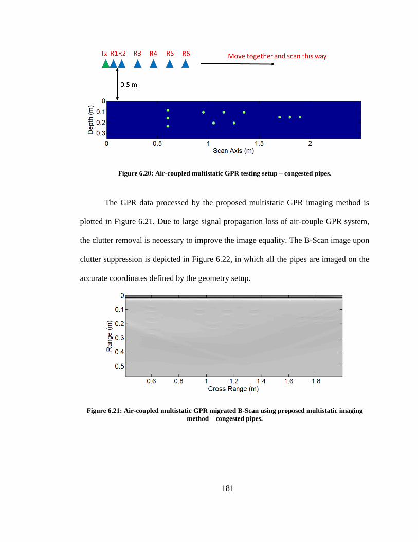
181

Figure 6.20: Air-coupled multistatic GPR testing setup – congested pipes.

The GPR data processed by the proposed multistatic GPR imaging method is

plotted in Figure 6.21. Due to large signal propagation loss of air-couple GPR system,

the clutter removal is necessary to improve the image equality. The B-Scan image upon

clutter suppression is depicted in Figure 6.22, in which all the pipes are imaged on the

accurate coordinates defined by the geometry setup.

Figure 6.21: Air-coupled multistatic GPR migrated B-Scan using proposed multistatic imaging

method – congested pipes.

182

Figure 6.22: Air-coupled multistatic GPR migrated B-Scan upon clutter removal – congested

pipes.

6.6. Conclusions

In this chapter, back-projection based imaging techniques are developed for both

ground-coupled multistatic GPR and air-coupled multistatic GPR systems. This

multistatic imaging method accounts for the height offsets of the antennas, spatial offsets

between antennas and refraction phenomenon at the air-ground interface. It fuses the

scattering signals gained from various antenna pairs and multiple radar cross sections to

produce migrated GPR image with higher SNR and SCR over conventional monostatic

or bistatic GPR systems. Experiments with simulation data indicate that the proposed

multistatic imaging method can effectively reconstruct the targets from raw GPR data.

6.7. References

[1] Multistatic Radar – Wikipedia: https://en.wikipedia.org/wiki/Multistatic_radar

[2] Counts, T., Gurbuz, A. C., Scott, W. R., McClellan, J. H., and Kim, K.,

“Multistatic ground-penetrating radar experiments,” IEEE Transactions on


[3] Inggs, M., Griffiths, H., Fioranelli, F., Ritchie, M., and Woodbridge, K.,

“Multistatic radar: System requirements and experimental validation,” In Radar

Conference (Radar), 2014 International, 1-6 (2014).

https://en.wikipedia.org/wiki/Multistatic_radar

183

[4] Yigit, E., Demirci, S., Ozdemir, C., and Kavak, A., “A synthetic aperture radar-

based focusing algorithm for B-Scan ground penetrating radar imagery,”

Microwave and Optical Technology Letters, 49(10), 2534 -2540 (2007).

[5] Charvat, G. L., “Small and short-range radar systems,” CRC Press, (2014).

[6] Charvat, G. L., “A Low-Power Radar Imaging System,” Ph.D. dissertation, Dept.

of Electrical and Computer Engineering, Michigan State University, East Lansing,

MI, (2007).

[7] Yang, H., Li, T., Li, N., He, Z., and Liu, Q. H., “Efficient Near-Field Imaging for

Single-Borehole Radar with Widely Separated Transceivers,” IEEE Transactions

on Geoscience and Remote Sensing, 53(10), 5327-5337 (2015).

[8] Vargas, J. M. M., “Signal processing techniques for radar based subsurface and

through wall imaging,” Doktora Tezi, University of Alberta, Edmonton, (2012).

[9] Demirci, S., Yigit, E., Eskidemir, I. H., and Ozdemir, C., “Ground penetrating

radar imaging of water leaks from buried pipes based on back-projection method,”

NDT & E International, 47, 35-42 (2012).

[10] Halman, J. I., Shubert, K. A., and Ruck, G. T., “SAR processing of ground-

penetrating radar data for buried UXO detection: results from a surface-based

system,” IEEE Transactions on Antennas and Propagation, 46(7), 1023-1027

(1998).

[11] Carin, L., Geng, N., McClure, M., Sichina, J., and Nguyen, L., “Ultra-wide-band

synthetic-aperture radar for mine-field detection,” IEEE Antennas and

Propagation Magazine, 41(1), 18-33 (1999).

[12] Gorham, L. A., and Moore, L. J., “SAR image formation toolbox for MATLAB,”

In Proc. SPIE, 7699, (2010).

[13] Yigit, E., Demirci, S., Özdemir, C., and Tekbaş, M, “Short-range ground-based

synthetic aperture radar imaging: performance comparison between frequency-

wavenumber migration and back-projection algorithms,” Journal of Applied

Remote Sensing, 7(1), 073483-073483 (2013).

[14] Zhuge, X., Savelyev, T. G., Yarovoy, A. G., Ligthart, L. P., and Levitas, B.,

“Comparison of different migration techniques for UWB short-range imaging,” In

Radar Conference, 2009. EuRAD 2009. European, 184-187 (2009).

[15] Chambers, D. H., Paglieroni, D. W., Mast, J. E., and Beer, N. R. “Real-Time

Vehicle-Mounted Multistatic Ground Penetrating Radar Imaging System for

Buried Object Detection,” (No. LLNL-TR-615452). Lawrence Livermore

National Laboratory (LLNL), Livermore, CA, (2013).

[16] Fischer, C., Herschlein, A., Younis, M., and Wiesbeck, W., “Detection of

antipersonnel mines by using the factorization method on multistatic ground-

penetrating radar measurements,” IEEE transactions on geoscience and remote

sensing, 45(1), 85-92 (2007).

184

[17] Kim, K., Gurbuz, A. C., Scott Jr, W. R., and McClellan, J. H., “A multi-static

ground-penetrating radar with an array of resistively loaded vee dipole antennas

for landmine detection,” In Defense and Security (pp. 495-506). International

Society for Optics and Photonics, (2005).

[18] Paglieroni, D. W., Chambers, D. H., Mast, J. E., Bond, S. W., and Beer, N. R.,

“Imaging modes for ground penetrating radar and their relation to detection

performance,” IEEE Journal of Selected Topics in Applied Earth Observations

and Remote Sensing, 8(3), 1132-1144 (2015).

[19] Karim, M. N. A., Malek, M. F. A., Jamlos, M. F., Seng, L. Y., and Saudin, N.,

“Design of ground penetrating radar antenna for buried object detection,” In RF

and Microwave Conference (RFM), 2013 IEEE International, 253-257 (2013).

[20] Labarthe, C., Mutzig, J. P., Jecko, B., Hamieh, H., Martinod, E., Feix, N., and

Vergnault, R, “An Ultra-Wideband radar concept for the detection of buried

victims beneath building rubble,” In Radar Conference-Surveillance for a Safer

World, 2009. RADAR. International, 1-6 (2009).

[21] Kim, K., and Scott, W. R., “Investigation of resistive vee antennas for a multi-

static ground-penetrating radar,” In Antennas and Propagation Society

International Symposium, 2005 IEEE, 96-99 (2005).

[22] Zhou, L., Huang, C., and Su, Y., “A fast back-projection algorithm based on cross

correlation for GPR imaging,” IEEE Geoscience and Remote Sensing Letters, 9(2),

228-232 (2012).

[23] Johansson, E. M., and Mast, J. E., “Three-dimensional ground penetrating radar

imaging using synthetic aperture time-domain focusing,” In Proc. SPIE, 2275,

205-214 (1994).

[24] Giannopoulos, A., “Modelling ground penetrating radar by GprMax,”

Construction and building materials, 19(10), 755-762 (2005).

[25] Zhang, Y., Burns, D., Orfeo, D., Huston, D. R., and Xia, T., “Rough ground

surface clutter removal in air-coupled ground penetrating radar data using low-

rank and sparse representation,” In SPIE Smart Structures and Materials+

Nondestructive Evaluation and Health Monitoring, 1016904, (2017).

185

CHAPTER 7: CONCLUSIONS AND FUTURE WORKS

7.1. Conclusions

In this dissertation, the three-stage cascade signal processing methodologies were

proposed to tackle with GPR signal processing from three perspectives: (1) Suppressing

the radar clutter signal through a low-rank and sparse representation based approach. (2)

Detecting the region of interest in the GPR image using Hilbert Transform and 2-D Renyi

entropy based statistical analysis to reduce the computational cost for further

sophisticated GPR data processing, such as back-projection migration. (3) Imaging the

underground target for both ground-coupled multistatic GPR and air-coupled multistatic

GPR configurations by back-projection imaging techniques. Experiments on both the

simulation and lab measurement data validate that the proposed three-stage cascade

signal processing methodologies can improve the performance of GPR system.

7.2. Future Work

The future work based on the materials presented in this dissertation can be

focused on a few directions.

In Chapter 2 and 3, the clutter removal problem is formulated as a low-rank and

sparse decomposition problem:

min𝐿,𝑆

‖𝐿‖∗ + 𝜆‖𝑆‖1 𝑠. 𝑡. 𝐷 = 𝐿 + 𝑆 (7.1)

The success of this decomposition is primarily dependent on how low the rank of matrix

𝐿 is and how sparse the matrix 𝑆 is. Some pre-processing steps can be applied to improve

the quality of the data prior to the decomposition and transform the decomposition

problem to the following one:

186

min𝐿,𝑆

‖𝐿‖∗ + 𝜆‖𝑆‖1 𝑠. 𝑡. 𝐷 = 𝐿 ∘ 𝜏 + 𝑆 ∘ 𝜌 (7.2)

where 𝜏 is the operator manipulating the clutter component in the GPR data to have lower

rank, and 𝜌 is the operator making the target component more sparse. The methodology

presented in Chapter 3 proposed the cross-correlation as the operator 𝜏 to align the ground

surface reflection and decrease the rank of the clutter matrix. A recent work in Ref. [1]

testified that instead of decomposing the raw GPR data, migration imaging can be applied

first to focus target response so that the sparsity and the strength of target response are

enhanced, which is a kind of the operator 𝜌 in Eq. (7.2). The future direction on the low-

rank and sparse representation based clutter removal can focus on optimizing and

implementing the operator 𝜏 and 𝜌 simultaneously for the GPR data matrix.

In Chapter 4 and 5, 2-D Renyi entropy analysis was performed on the amplitude

and phase information of the GPR data. For GPR underground sensing application, most

of the targets are objects with certain shapes, so geometry structure and morphological

information reside inside the GPR data matrix. The 2-D entropy analysis methodology

can be further explored and applied on the data features extracted from morphological

transformation, such as Curvelet Transform [2]-[5] to afford more comprehensive region

of interest detection.

For GPR migration problem, the propagating velocity of the EM wave in

subsurface media is a vital input, which is associated with the dielectric constant of the

subsurface media. Unfortunately, this is usually not prior information for real field GPR

testing. The approaches for measuring or estimating the dielectric constant and wave

velocity information have been investigated by some research work [6]-[8] for

187

homogeneous subsurface media. However, for most of the real GPR testing scenarios,

the subsurface media is inhomogeneous. Moreover, Ref. [9]-[10] claims that the

systematic errors in the migration techniques may lead to poor image reconstruction and

inaccurate target position estimation even if the exact velocity distribution is used as the

prior knowledge. Therefore, autofocusing technique for GPR imaging is highly

demanded and will be investigated in the future work.

7.3. References

[1] Song, X., Xiang, D., Zhou, K., & Su, Y. (2017). Improving RPCA-Based Clutter

Suppression in GPR Detection of Antipersonnel Mines. IEEE Geoscience and

Remote Sensing Letters.

[2] Terrasse, G., Nicolas, J. M., Trouvé, E., & Drouet, É. (2015, July). Application of

the curvelet transform for pipe detection in GPR images. In Geoscience and

Remote Sensing Symposium (IGARSS), 2015 IEEE International (pp. 4308-4311).

IEEE.

[3] Tzanis, A. (2015). The Curvelet Transform in the analysis of 2-D GPR data: Signal

enhancement and extraction of orientation-and-scale-dependent information.

Journal of Applied Geophysics, 115, 145-170.

[4] Temlioglu, E., & Erer, I. (2016). Clutter removal in ground-penetrating radar

images using morphological component analysis. IEEE Geoscience and Remote


[5] Bao, Q. Z., Li, Q. C., & Chen, W. C. (2014). GPR data noise attenuation on the

curvelet transform. Applied Geophysics, 11(3), 301-310.

[6] Soldovieri, F., Prisco, G., & Persico, R. (2009). A strategy for the determination

of the dielectric permittivity of a lossy soil exploiting GPR surface measurements

and a cooperative target. Journal of Applied Geophysics, 67(4), 288-295.

[7] Huston, D. (2010). Structural sensing, health monitoring, and performance

evaluation. CRC Press.

[8] Brown, J., Nichols, J., Steinbronn, L., & Bradford, J. (2009). Improved GPR

interpretation through resolution of lateral velocity heterogeneity: example from

an archaeological site investigation. Journal of Applied Geophysics, 68(1), 3-8.

[9] Black, J. L., & Brzostowski, M. A. (1994). Systematics of time-migration errors.

Geophysics, 59(9), 1419-1434.

[10] Wei, X., & Zhang, Y. (2014). Autofocusing techniques for GPR data from RC

bridge decks. IEEE Journal of Selected Topics in Applied Earth Observations and

Remote Sensing, 7(12), 4860-4868.

189

BIBLIOGRAPHY

2013 Report Card for America’s Infrastructure, American Society of Civil Engineers:

http://2013.infrastructurereportcard.org/

Addison, A. D., Battista, B. M., & Knapp, C. C. (2009). Improved hydrogeophysical

parameter estimation from empirical mode decomposition processed ground

penetrating radar data. Journal of Environmental & Engineering Geophysics, 14(4),

171-178.

Ahmed, A., Zhang, Y., Burns, D., Huston, D., & Xia, T. (2016). Design of UWB antenna

for air-coupled impulse ground-penetrating radar. IEEE Geoscience and Remote


AI-Qadi, I., Lahouar, S., Jiang, K., McGhee, K., & Mokarem, D. (2005). Accuracy of

ground-penetrating radar for estimating rigid and flexible pavement layer

thicknesses. Transportation Research Record: Journal of the Transportation Research

Board, (1940), 69-78.

Alani, A. M., Aboutalebi, M., & Kilic, G. (2013). Applications of ground penetrating

radar (GPR) in bridge deck monitoring and assessment. Journal of Applied

Geophysics, 97, 45-54.

Al-Qadi, I. L., Xie, W., & Roberts, R. (2008). Scattering analysis of ground-penetrating

radar data to quantify railroad ballast contamination. NDT & E International, 41(6),

441-447.

Al-Qadi, I. L., Xie, W., Roberts, R., & Leng, Z. (2010). Data analysis techniques for GPR

used for assessing railroad ballast in high radio-frequency environment. Journal of

transportation engineering, 136(4), 392-399.

Amaldi, E., & Kann, V. (1998). On the approximability of minimizing nonzero variables

or unsatisfied relations in linear systems. Theoretical Computer Science, 209(1-2),

237-260.

Amin, M. G. (Ed.). (2016). Through-the-wall radar imaging. CRC press.

Annan, A. P. (1999). Practical processing of GPR data. Sensors and software, Ontario.

Aydin, E., & Yüksel, S. E. (2017, May). Buried target detection with ground penetrating

radar using deep learning method. In Signal Processing and Communications

Applications Conference (SIU), 2017 25th (pp. 1-4). IEEE.

Baili, J., Lahouar, S., Hergli, M., Al-Qadi, I. L., & Besbes, K. (2009). GPR signal de-

noising by discrete wavelet transform. Ndt & E International, 42(8), 696-703.

Bano, M., Marquis, G., Nivière, B., Maurin, J., & Cushing, M. (2000). Investigating

alluvial and tectonic features with ground-penetrating radar and analyzing

diffractions patterns. Journal of Applied Geophysics, 43(1), 33-41.

Bao, Q. Z., Li, Q. C., & Chen, W. C. (2014). GPR data noise attenuation on the curvelet

transform. Applied Geophysics, 11(3), 301-310.

190

Baraniuk, R. G., Flandrin, P., Janssen, A. J., & Michel, O. J. (2001). Measuring time-

frequency information content using the Rényi entropies. IEEE Transactions on

Information Theory, 47(4), 1391-1409.

Basile, V., Carrozzo, M. T., Negri, S., Nuzzo, L., Quarta, T., & Villani, A. V. (2000). A

ground-penetrating radar survey for archaeological investigations in an urban area

(Lecce, Italy). Journal of Applied Geophysics, 44(1), 15-32.

Battista, B. M., Knapp, C., McGee, T., & Goebel, V. (2007). Application of the empirical

mode decomposition and Hilbert-Huang transform to seismic reflection data.

Geophysics, 72(2), H29-H37.

Becker, J., Havens, T. C., Pinar, A., & Schulz, T. J. (2015, May). Deep belief networks

for false alarm rejection in forward-looking ground-penetrating radar. In SPIE

Defense+ Security (pp. 94540W-94540W). International Society for Optics and

Photonics.

Becker, S. R., Candès, E. J., & Grant, M. C. (2011). Templates for convex cone problems

with applications to sparse signal recovery. Mathematical programming computation,

3(3), 165-218.

Benson, A. K. (1995). Applications of ground penetrating radar in assessing some

geological hazards: examples of groundwater contamination, faults, cavities. Journal

of applied Geophysics, 33(1-3), 177-193.

Besaw, L. E., & Stimac, P. J. (2014, May). Deep learning algorithms for detecting

explosive hazards in ground penetrating radar data. In Proc. SPIE (Vol. 9072, p.

90720Y).

Besaw, L. E., & Stimac, P. J. (2015, May). Deep convolutional neural networks for

classifying GPR B-scans. In SPIE Defense+ Security (pp. 945413-945413).

International Society for Optics and Photonics.

Bettigole, N., & Robinson, R. (1997). Bridge Decks. American Society of Civil

Engineers, New York.

Black, J. L., & Brzostowski, M. A. (1994). Systematics of time-migration errors.

Geophysics, 59(9), 1419-1434.

Bleistein, N. (1987). On the imaging of reflectors in the earth. Geophysics, 52(7), 931-

942.

Bourgeois, J. M., & Smith, G. S. (1996). A fully three-dimensional simulation of a

ground-penetrating radar: FDTD theory compared with experiment. IEEE

Transactions on Geoscience and Remote Sensing, 34(1), 36-44.

Bouzerdoum, A., Tivive, F. H. C., & Abeynayake, C. (2016, May). Target detection in

GPR data using joint low-rank and sparsity constraints. In SPIE Commercial+

Scientific Sensing and Imaging (pp. 98570A-98570A). International Society for

Optics and Photonics.

Bralich, J., Reichman, D., Collins, L. M., & Malof, J. M. (2017, May). Improving

convolutional neural networks for buried threat in ground penetrating radar using

transfer learning via pretraining. In SPIE Defense+ Security (pp. 101820X-

101820X). International Society for Optics and Photonics.

191

Brown, J., Nichols, J., Steinbronn, L., & Bradford, J. (2009). Improved GPR

interpretation through resolution of lateral velocity heterogeneity: example from an

archaeological site investigation. Journal of Applied Geophysics, 68(1), 3-8.

Cafforio, C., Prati, C., & Rocca, F. (1991). Full resolution focusing of SEASAT SAR

images in the frequency-wave number domain. International Journal of Remote

Sensing, 12(3), 491-510.

Cafforio, C., Prati, C., & Rocca, F. (1991). SAR data focusing using seismic migration

techniques. IEEE transactions on aerospace and electronic systems, 27(2), 194-207.

Camilo, J. A., Malof, J. M., & Collins, L. M. (2016, May). A feature learning approach

for classifying buried threats in forward looking ground penetrating radar data. In

Proc. SPIE (Vol. 9823, p. 98231I).

Candès, E. J., Li, X., Ma, Y., & Wright, J. (2011). Robust principal component analysis?.

Journal of the ACM (JACM), 58(3), 11.

Candra, P., Xia, T., Huston, D., & Wang, G. (2013, April). Two dimensional entropy and

short time Fourier transform application on ground penetrating radar data analysis.

In SPIE Smart Structures and Materials+ Nondestructive Evaluation and Health

Monitoring (pp. 86940J-86940J). International Society for Optics and Photonics.

Cardimona, S. J., Clement, W. P., & Kadinsky-Cade, K. (1998). Seismic reflection and

ground-penetrating radar imaging of a shallow aquifer. Geophysics, 63(4), 1310-

1317.

Carin, L., Geng, N., McClure, M., Sichina, J., & Nguyen, L. (1999). Ultra-wide-band

synthetic-aperture radar for mine-field detection. IEEE Antennas and Propagation

Magazine, 41(1), 18-33.

Cassidy, N. J. (2007). Evaluating LNAPL contamination using GPR signal attenuation

analysis and dielectric property measurements: Practical implications for

hydrological studies. Journal of Contaminant Hydrology, 94(1), 49-75.

Cassidy, N. J. (2009). Ground penetrating radar data processing, modelling and analysis.

Ground penetrating radar: theory and applications, 141-176.

Cervone, G., & Haack, B. (2012). Supervised machine learning of fused RADAR and

optical data for land cover classification. Journal of Applied Remote Sensing, 6(1),

063597-063597.

Chambers, D. H., Paglieroni, D. W., Mast, J. E., & Beer, N. R. (2013). Real-Time

Vehicle-Mounted Multistatic Ground Penetrating Radar Imaging System for Buried

Object Detection (No. LLNL-TR-615452). Lawrence Livermore National

Laboratory (LLNL), Livermore, CA.

Charvat, G. L. (2007). A Low-Power Radar Imaging System (Doctoral dissertation,

Michigan State University).

Charvat, G. L. (2014). Small and short-range radar systems. CRC Press.

Chernyak, V. S. (1998). Fundamentals of multisite radar systems: multistatic radars and

multistatic radar systems. CRC Press.

192

Claerbout, J. F. (1986). Imaging the Earth's interior. Geophysical Journal International,

86(1), 217-217.

Collins, L. M., Torrione, P. A., Munshi, V. S., Throckmorton, C. S., Zhu, Q. E.,

Clodfelter, J. F., & Frasier, S. (2002, August). Algorithms for landmine detection

using the NIITEK ground penetrating radar. In Proc. SPIE (Vol. 4742, pp. 709-718).

Conyers, L. B. (2013). Ground-penetrating radar for archaeology. AltaMira Press.

Cook, J. C. (1975). Radar transparencies of mine and tunnel rocks. Geophysics, 40(5),

865-885.

Counts, T., Gurbuz, A. C., Scott, W. R., McClellan, J. H., & Kim, K. (2007). Multistatic

ground-penetrating radar experiments. IEEE Transactions on Geoscience and

Remote Sensing, 45(8), 2544-2553.

Crooks, W. T., & Cheke, R. A. (2014). Soil moisture assessments for brown locust

Locustana pardalina breeding potential using synthetic aperture radar. Journal of

Applied Remote Sensing, 8(1), 084898-084898.

Dang, C., & Radha, H. (2015). RPCA-KFE: Key frame extraction for video using robust

principal component analysis. IEEE Transactions on Image Processing, 24(11),

3742-3753.

Daniels, D. J. (1994). Surface penetrating radar for industrial and security applications.

Microwave Journal, 37(12), 68-76.

Daniels, D. J. (ed.). (2004) Ground Penetrating Radar (2nd ed.). Institution of

Engineering and Technology (IET).

Degenhardt, J. J., & Giardino, J. R. (2003). Subsurface investigation of a rock glacier

using ground‐penetrating radar: Implications for locating stored water on Mars.

Journal of Geophysical Research: Planets, 108(E4).

Demirci, S., Yigit, E., Eskidemir, I. H., & Ozdemir, C. (2012). Ground penetrating radar

imaging of water leaks from buried pipes based on back-projection method. NDT &

E International, 47, 35-42.

Desai, M. D., & Jenkins, W. K. (1992). Convolution backprojection image reconstruction

for spotlight mode synthetic aperture radar. IEEE Transactions on Image Processing,

1(4), 505-517.

Entropy (information theory):

https://www.princeton.edu/~achaney/tmve/wiki100k/docs/Entropy_%28informatio

n_theory%29.html

Evans, S. (1963). Radio techniques for the measurement of ice thickness. Polar Record,

11(73), 406-410.

Federal Transit Administration Asset Management Guide, October 2012, FTA Report

No. 0027:


193

Ferrario, M., Signorini, M. G., Magenes, G., & Cerutti, S. (2006). Comparison of

entropy-based regularity estimators: application to the fetal heart rate signal for the

identification of fetal distress. IEEE Transactions on Biomedical Engineering, 53(1),

119-125.

Fischer, C., Herschlein, A., Younis, M., & Wiesbeck, W. (2007). Detection of

antipersonnel mines by using the factorization method on multistatic ground-

penetrating radar measurements. IEEE transactions on geoscience and remote

sensing, 45(1), 85-92.

Fisher, E., McMechan, G. A., & Annan, A. P. (1992). Acquisition and processing of

wide-aperture ground-penetrating radar data. Geophysics, 57(3), 495-504.

Fruehauf, F., Heilig, A., Schneebeli, M., Fellin, W., & Scherzer, O. (2009). Experiments

and algorithms to detect snow avalanche victims using airborne ground-penetrating

radar. IEEE Transactions on Geoscience and Remote Sensing, 47(7), 2240-2251.

Gader, P., Lee, W. H., & Wilson, J. N. (2004). Detecting landmines with ground-

penetrating radar using feature-based rules, order statistics, and adaptive whitening.

IEEE Transactions on Geoscience and Remote Sensing, 42(11), 2522-2534.

Gamba, P., & Lossani, S. (2000). Neural detection of pipe signatures in ground

penetrating radar images. IEEE Transactions on Geoscience and Remote Sensing,

38(2), 790-797.

Gazdag, J. (1978). Wave equation migration with the phase-shift method. Geophysics,

43(7), 1342-1351.

Gazdag, J., & Sguazzero, P. (1984). Migration of seismic data. Proceedings of the IEEE,

72(10), 1302-1315.

Gerlitz, K., Knoll, M. D., Cross, G. M., Luzitano, R. D., & Knight, R. (1993, April).

Processing ground penetrating radar data to improve resolution of near-surface

targets. In 6th EEGS Symposium on the Application of Geophysics to Engineering

and Environmental Problems.

Ghose, R., & Slob, E. C. (2006). Quantitative integration of seismic and GPR reflections

to derive unique estimates for water saturation and porosity in subsoil. Geophysical

Research Letters, 33(5).

Giannopoulos, A. (2005). Modelling ground penetrating radar by GprMax. Construction

and building materials, 19(10), 755-762.

Gilmore, C., Jeffrey, I., & LoVetri, J. (2006). Derivation and comparison of SAR and

frequency-wavenumber migration within a common inverse scalar wave problem

formulation. IEEE transactions on geoscience and remote sensing, 44(6), 1454-1461.

Goodman, D. (1994). Ground-penetrating radar simulation in engineering and

archaeology. Geophysics, 59(2), 224-232.

Gorham, L. A., & Moore, L. J. (2010, April). SAR image formation toolbox for

MATLAB. In Proc. SPIE (Vol. 7699, p. 769906).

GPR Processing Software – MALA Ground Penetrating Radar – GPR:


194

Grazzini, G., Pieraccini, M., Parrini, F., Spinetti, A., Macaluso, G., Dei, D., & Atzeni, C.

(2010, June). An ultra-wideband high-dynamic range GPR for detecting buried

people after collapse of buildings. In Ground Penetrating Radar (GPR), 2010 13th

International Conference on (pp. 1-6). IEEE.

Ground Penetrating Radar Data Acquisition Unit – SIR 30 – GSSI:


Ground Penetrating Radar for Bridge Deck Inspection, Geophysical Survey Systems,

Inc.: http://www.geophysical.com/bridgeinspection.htm

Ground Penetrating Radar: https://en.wikipedia.org/wiki/Ground-penetrating_radar

Gu, K., Wang, G., & Li, J. (2004). Migration based SAR imaging for ground penetrating

radar systems. IEE Proceedings-Radar, Sonar and Navigation, 151(5), 317-325.

Gunawardena, A., & Longstaff, D. (1998). Wave equation formulation of synthetic

aperture radar (SAR) algorithms in the time-space domain. IEEE transactions on

Geoscience and Remote Sensing, 36(6), 1995-1999.

Halman, J. I., Shubert, K. A., & Ruck, G. T. (1998). SAR processing of ground-

penetrating radar data for buried UXO detection: results from a surface-based system.

IEEE Transactions on Antennas and Propagation, 46(7), 1023-1027.

Han, J., & van der Baan, M. (2013). Empirical mode decomposition for seismic time-

frequency analysis. Geophysics.

Hanmandlu, M., Verma, O. P., Kumar, N. K., & Kulkarni, M. (2009). A novel optimal

fuzzy system for color image enhancement using bacterial foraging. IEEE

Transactions on Instrumentation and Measurement, 58(8), 2867-2879.

Hintz, K. J. (2004, September). SNR improvements in NIITEK ground-penetrating radar.

In Defense and Security (pp. 399-408). International Society for Optics and

Photonics.

History of Ground Penetrating Radar (GPR): https://www.obonic.de/article/ground-

peentrating-radar-history/

Ho, K. C., Carin, L., Gader, P. D., & Wilson, J. N. (2008). An investigation of using the

spectral characteristics from ground penetrating radar for landmine/clutter

discrimination. IEEE transactions on Geoscience and Remote Sensing, 46(4), 1177-

1191.

Hodson, T., Gooch, D. L., & Stuart, G. W. (1997). Structures within the surge front at

Bakaninbreen, Svalbard, using ground-penetrating radar. Annals of Glaciology, 24,

122-129.

Huisman, J. A., Hubbard, S. S., Redman, J. D., & Annan, A. P. (2003). Measuring soil

water content with ground penetrating radar. Vadose zone journal, 2(4), 476-491.

Huisman, J. A., Sperl, C., Bouten, W., & Verstraten, J. M. (2001). Soil water content

measurements at different scales: accuracy of time domain reflectometry and ground-

penetrating radar. Journal of Hydrology, 245(1), 48-58.

Hulsenbeck, et al. (1926) German Pat. No. 489434.

195

Huston, D. (2010). Structural sensing, health monitoring, and performance evaluation.

CRC Press.

Huston, D., Hu, J. Q., Maser, K., Weedon, W., & Adam, C. (2000). GIMA ground

penetrating radar system for monitoring concrete bridge decks. Journal of Applied

Geophysics, 43(2), 139-146.

Huston, D., Xia, T., Zhang, Y., Fan, T., Orfeo, D., & Razinger, J. (2017, April). Urban

underground infrastructure mapping and assessment. In SPIE Smart Structures and

Materials+ Nondestructive Evaluation and Health Monitoring (pp. 101680M-

101680M). International Society for Optics and Photonics.

Inggs, M., Griffiths, H., Fioranelli, F., Ritchie, M., & Woodbridge, K. (2014, October).

Multistatic radar: System requirements and experimental validation. In Radar

Conference (Radar), 2014 International (pp. 1-6). IEEE.

Irving, J. D., & Knight, R. J. (2003). Removal of wavelet dispersion from ground-

penetrating radar data. Geophysics, 68(3), 960-970.

Jeng, Y., Lin, C. H., Li, Y. W., Chen, C. S., & Yu, H. M. (2011). Application of sub-

image multiresolution analysis of Ground-penetrating radar data in a study of shallow

structures. Journal of Applied Geophysics, 73(3), 251-260.

Jia, S., Zhang, X., & Li, Q. (2015). Spectral–Spatial Hyperspectral Image Classification

Using $\ell_ {1/2} $ Regularized Low-Rank Representation and Sparse

Representation-Based Graph Cuts. IEEE Journal of Selected Topics in Applied Earth

Observations and Remote Sensing, 8(6), 2473-2484.

Jiankui, Z., Zishu, H., Sellathurai, M., & Hongming, L. (2008). Modified Hough

transform for searching radar detection. IEEE Geoscience and Remote Sensing

Letters, 5(4), 683-686.

Johansson, E. M., & Mast, J. E. (1994, September). Three-dimensional ground

penetrating radar imaging using synthetic aperture time-domain focusing. In Proc.

SPIE (Vol. 2275, pp. 205-214).

Jol, H. M. (Ed.). (2008). Ground penetrating radar theory and applications. elsevier.

Kadaba, P. K. (1976). Penetration of 0.1 GHz to 1.5 GHz electromagnetic waves into the

earth surface for remote sensing applications. In Engineering in a Changing Economy

(pp. 48-50).

Kalika, D., Knox, M. T., Collins, L. M., Torrione, P. A., & Morton, K. D. (2015, May).

Leveraging robust principal component analysis to detect buried explosive threats in

handheld ground-penetrating radar data. In SPIE Defense+ Security (pp. 94541D-

94541D). International Society for Optics and Photonics.

Karim, M. N. A., Malek, M. F. A., Jamlos, M. F., Seng, L. Y., & Saudin, N. (2013,

December). Design of ground penetrating radar antenna for buried object detection.

In RF and Microwave Conference (RFM), 2013 IEEE International (pp. 253-257).

IEEE.

196

Karlsen, B., Larsen, J., Sorensen, H. B. D., & Jakobsen, K. B. (2001). Comparison of

PCA and ICA based clutter reduction in GPR systems for anti-personal landmine

detection. In Statistical Signal Processing, 2001. Proceedings of the 11th IEEE Signal

Processing Workshop on (pp. 146-149). IEEE.

Karlsen, B., Sørensen, H. B. D., Larsen, J., & Jackobsen, K. B. (2002, August).

Independent component analysis for clutter reduction in ground penetrating radar

data. In Proceedings of the SPIE, AeroSense (pp. 378-389).

Kassem, E., Chowdhury, A., Scullion, T., & Masad, E. (2016). Application of ground-

penetrating radar in measuring the density of asphalt pavements and its relationship

to mechanical properties. International Journal of Pavement Engineering, 17(6), 503-

516.

Kenley, E. C., & Cho, Y. R. (2011, December). Entropy-based graph clustering:

Application to biological and social networks. In Data Mining (ICDM), 2011 IEEE

11th International Conference on (pp. 1116-1121). IEEE.

Kim, K., & Scott, W. R. (2005, July). Investigation of resistive vee antennas for a multi-

static ground-penetrating radar. In Antennas and Propagation Society International

Symposium, 2005 IEEE (Vol. 3, pp. 96-99). IEEE.

Kim, K., Gurbuz, A. C., Scott Jr, W. R., & McClellan, J. H. (2005, June). A multi-static

ground-penetrating radar with an array of resistively loaded vee dipole antennas for

landmine detection. In Defense and Security (pp. 495-506). International Society for


Krause, V., Abdel-Qader, I., Abudayyeh, O., & Yehia, S. (2007, May). An image

segmentation algorithm for the detection of rebar in bridge decks from GPR scans.

In Electro/Information Technology, 2007 IEEE International Conference on (pp.

114-119). IEEE.

Labarthe, C., Mutzig, J. P., Jecko, B., Hamieh, H., Martinod, E., Feix, N., ... & Vergnault,

R. (2009, October). An Ultra-Wideband radar concept for the detection of buried

victims beneath building rubble. In Radar Conference-Surveillance for a Safer

World, 2009. RADAR. International (pp. 1-6). IEEE.

Lahouar, S., & Al-Qadi, I. L. (2008). Automatic detection of multiple pavement layers

from GPR data. NDT & e International, 41(2), 69-81.

Lai, W. L., & Poon, C. S. (2012, June). GPR data analysis in time-frequency domain. In

Ground Penetrating Radar (GPR), 2012 14th International Conference on (pp. 362-

366). IEEE.

Lai, W. L., Kind, T., & Wiggenhauser, H. (2011). Using ground penetrating radar and

time–frequency analysis to characterize construction materials. NDT & E

International, 44(1), 111-120.

Lambot, S., Slob, E. C., van den Bosch, I., Stockbroeckx, B., & Vanclooster, M. (2004).

Modeling of ground-penetrating radar for accurate characterization of subsurface

electric properties. IEEE transactions on geoscience and remote sensing, 42(11),

2555-2568.

197

Lambot, S., Weihermüller, L., Huisman, J. A., Vereecken, H., Vanclooster, M., & Slob,

E. C. (2006). Analysis of air‐launched ground‐penetrating radar techniques to

measure the soil surface water content. Water resources research, 42(11).

Le Bastard, C., Wang, Y., Baltazart, V., & Derobert, X. (2014). Time delay and

permittivity estimation by ground-penetrating radar with support vector regression.

IEEE Geoscience and Remote Sensing Letters, 11(4), 873-877.

Leckebusch, J. (2003). Ground‐penetrating radar: a modern three‐dimensional

prospection method. Archaeological prospection, 10(4), 213-240.

Lecomte, I., Hamran, S. E., & Gelius, L. J. (2005). Improving Kirchhoff migration with

repeated local plane‐wave imaging? A SAR‐inspired signal‐processing approach in

prestack depth imaging. Geophysical Prospecting, 53(6), 767-785.

Lee, J. S., Nguyen, C., & Scullion, T. (2004). A novel, compact, low-cost, impulse

ground-penetrating radar for nondestructive evaluation of pavements. IEEE

Transactions on Instrumentation and Measurement, 53(6), 1502-1509.

Leng, Z., & Al-Qadi, I. (2010). Railroad Ballast Evaluation Using Ground-Penetrating

Radar: Laboratory Investigation and Field Validation. Transportation Research

Record: Journal of the Transportation Research Board, (2159), 110-117.

Leng, Z., & Al-Qadi, I. L. (2009). Dielectric constant measurement of railroad ballast

and application of STFT for GPR data analysis. Non-Destructive Testing in Civil

Engineering Nantes, sn.

Lester, J., & Bernold, L. E. (2007). Innovative process to characterize buried utilities

using ground penetrating radar. Automation in Construction, 16(4), 546-555.

Leucci, G. (2008). Ground penetrating radar: the electromagnetic signal attenuation and

maximum penetration depth. Scholarly research exchange, 2008.

Li, J., Zollinger, D., & Lytton, R. (2008). Detection of delamination in concrete

pavements using ground-coupled ground-penetrating radar technique. Transportation

Research Record: Journal of the Transportation Research Board, (2087), 68-77.

Li, L., Tan, A. E. C., Jhamb, K., & Rambabu, K. (2012). Buried object characterization

using ultra-wideband ground penetrating radar. IEEE Transactions on Microwave

Theory and Techniques, 60(8), 2654-2664.

Li, Z., & Crocker, M. J. (2006). A study of joint time-frequency analysis-based modal

analysis. IEEE transactions on instrumentation and measurement, 55(6), 2335-2342.

Liu, H., Birken, R., & Wang, M. L. (2016). Automatic pavement layer identification with

multichannel ground penetrating radar at traffic speed. Journal of Applied Remote

Sensing, 10(4), 046023-046023.

Liu, L., & Liu, S. (2014). Remote detection of human vital sign with stepped-frequency

continuous wave radar. IEEE Journal of Selected Topics in Applied Earth

Observations and Remote Sensing, 7(3), 775-782.

Liu, L., Liu, Z., & Barrowes, B. E. (2011). Through-wall bio-radiolocation with UWB

impulse radar: Observation, simulation and signal extraction. IEEE Journal of

Selected Topics in Applied Earth Observations and Remote Sensing, 4(4), 791-798.

198

Loizos, A., & Plati, C. (2007). Accuracy of ground penetrating radar horn-antenna

technique for sensing pavement subsurface. IEEE Sensors Journal, 7(5), 842-850.

Loizos, A., & Plati, C. (2007). Accuracy of pavement thicknesses estimation using

different ground penetrating radar analysis approaches. NDT & e International, 40(2),

147-157.

Lu, Q., Pu, J., & Liu, Z. (2014). Feature extraction and automatic material classification

of underground objects from ground penetrating radar data. Journal of Electrical and

Computer Engineering, 2014, 28.

Lunt, I. A., Hubbard, S. S., & Rubin, Y. (2005). Soil moisture content estimation using

ground-penetrating radar reflection data. Journal of Hydrology, 307(1), 254-269.

Maas, C., & Schmalzl, J. (2013). Using pattern recognition to automatically localize

reflection hyperbolas in data from ground penetrating radar. Computers &

geosciences, 58, 116-125.

Machguth, H., Eisen, O., Paul, F., & Hoelzle, M. (2006). Strong spatial variability of

snow accumulation observed with helicopter‐borne GPR on two adjacent Alpine

glaciers. Geophysical research letters, 33(13).

Maierhofer, C. (2003). Nondestructive evaluation of concrete infrastructure with ground

penetrating radar. Journal of Materials in Civil Engineering, 15(3), 287-297.

Malagodi, S., Orlando, L., & Piro, S. (1996, September). Approaches to increase

resolution of radar signal. In Proceedings of 6th international conference on ground

penetrating radar. Tohoku University, Sendai (pp. 283-288).

Masarik, M. P., Burns, J., Thelen, B. T., Kelly, J., & Havens, T. C. (2015, May). GPR

anomaly detection with robust principal component analysis. In Proc. SPIE (Vol.

9454, pp. 945414-945414).

Maser, K. R. (2009, June). Integration of ground penetrating radar and infrared

thermography for bridge deck condition evaluation. In Non-Destructive Testing in

Civil Engineering Conference, Nantes, France, June 30th-July 3rd.

Mason, E., Yonel, B., & Yazici, B. (2017, May). Deep learning for radar. In Radar

Conference (RadarConf), 2017 IEEE (pp. 1703-1708). IEEE.

MATGPR Home: http://users.uoa.gr/~atzanis/matgpr/matgpr.html

Miller, D., Oristaglio, M., & Beylkin, G. (1987). A new slant on seismic imaging:

Migration and integral geometry. Geophysics, 52(7), 943-964.

Milman, A. S. (1993). SAR imaging by ω—κ migration. International Journal of Remote

Sensing, 14(10), 1965-1979.

Mitra, S. K., & Kuo, Y. (2006). Digital signal processing: a computer-based approach

(Vol. 2). McGraw-Hill Higher Education.

Monostatic radar – Wikipedia: https://en.wikipedia.org/wiki/Monostatic_radar

Multistatic radar – Wikipedia: https://en.wikipedia.org/wiki/Multistatic_radar

Munson, D. C., O'Brien, J. D., & Jenkins, W. K. (1983). A tomographic formulation of

spotlight-mode synthetic aperture radar. Proceedings of the IEEE, 71(8), 917-925.

199

Murray, T., Booth, A., & Rippin, D. M. (2007). Water-content of glacier-ice: Limitations

on estimates from velocity analysis of surface ground-penetrating radar surveys.

Journal of Environmental & Engineering Geophysics, 12(1), 87-99.

Narayanan, R. M., Jakub, J. W., Li, D., & Elias, S. E. (2004). Railroad track modulus

estimation using ground penetrating radar measurements. NDT & E International,

37(2), 141-151.

Nezlin, D. V., Kostylev, V. I., Blyakhman, A. B., Ryndyk, A. G., & Myakinkov, A. V.

(2007). Bistatic radar: principles and practice. John Wiley & Sons.

Ni, S. H., Huang, Y. H., Lo, K. F., & Lin, D. C. (2010). Buried pipe detection by ground

penetrating radar using the discrete wavelet transform. Computers and Geotechnics,

37(4), 440-448.

Nilsson, S., & Andersson, L. E. (1998, September). Application of fast back-projection

techniques for some inverse problems of synthetic aperture radar. In

Aerospace/Defense Sensing and Controls (pp. 62-72). International Society for


Nobes, D. C. (1999). Geophysical surveys of burial sites: a case study of the Oaro urupa.

Geophysics, 64(2), 357-367.

Olhoeft, G. R. (2000). Maximizing the information return from ground penetrating radar.

Journal of Applied Geophysics, 43(2), 175-187.

Otsu, N. (1979). A threshold selection method from gray-level histograms. IEEE

transactions on systems, man, and cybernetics, 9(1), 62-66.

Ozdemir, C., Demirci, S., & Yigit, E. (2008). Practical algorithms to focus B-scan GPR

images: Theory and application to real data. Progress In Electromagnetics Research

B, 6, 109-122.

Ozdemir, C., Demirci, S., Yigit, E., & Kavak, A. (2007). A hyperbolic summation

method to focus B‐scan ground penetrating radar images: An experimental study with

a stepped frequency system. Microwave and Optical Technology Letters, 49(3), 671-

676.

Özdemir, C., Demirci, Ş., Yiğit, E., & Yilmaz, B. (2014). A review on migration methods

in B-scan ground penetrating radar imaging. Mathematical Problems in Engineering,

2014.

Paglieroni, D. W., Chambers, D. H., Mast, J. E., Bond, S. W., & Beer, N. R. (2015).

Imaging modes for ground penetrating radar and their relation to detection

performance. IEEE Journal of Selected Topics in Applied Earth Observations and

Remote Sensing, 8(3), 1132-1144.

Peng, Y., Ganesh, A., Wright, J., Xu, W., & Ma, Y. (2012). RASL: Robust alignment by

sparse and low-rank decomposition for linearly correlated images. IEEE Transactions

on Pattern Analysis and Machine Intelligence, 34(11), 2233-2246.

Pinel, N., Le Bastard, C., Baltazart, V., Bourlier, C., & Wang, Y. (2011). Influence of

layer roughness for road survey by ground penetrating radar at nadir: theoretical

study. IET radar, sonar & navigation, 5(6), 650-656.

200

Pipan, M., Baradello, L., Forte, E., Prizzon, A., & Finetti, I. (1999). 2-D and 3-D

processing and interpretation of multi-fold ground penetrating radar data: a case

history from an archaeological site. Journal of Applied geophysics, 41(2), 271-292.

Potin, D., Duflos, E., & Vanheeghe, P. (2006). Landmines ground-penetrating radar

signal enhancement by digital filtering. IEEE Transactions on Geoscience and

Remote Sensing, 44(9), 2393-2406.

RADAN® - GPR Software by GSSI: http://www.geophysical.com/software.htm

Radar Basics – Range Resolution:


Richards, M. A. (2005). Fundamentals of radar signal processing. Tata McGraw-Hill

Education.

Rodríguez-Abad, I., Martínez-Sala, R., García-García, F., & Capuz-Lladró, R. (2010).

Non-destructive methodologies for the evaluation of moisture content in sawn timber

structures: ground-penetrating radar and ultrasound techniques. Near Surface

Geophysics, 8(6), 475-482.

Roe, K. C., & Ellerbruch, D. A. (1979). Development and testing of a microwave system

to measure coal layer thickness up to 25 cm (No. FE-8881-1; SR-723-8-79). National

Bureau of Standards, Boulder, CO (USA). Electromagnetic Fields Div..

Saarenketo, T., & Scullion, T. (2000). Road evaluation with ground penetrating radar.

Journal of applied geophysics, 43(2), 119-138.

Safont, G., Salazar, A., Rodriguez, A., & Vergara, L. (2014). On recovering missing

ground penetrating radar traces by statistical interpolation methods. Remote Sensing,

6(8), 7546-7565.

Sakaguchi, R. T., Morton, K. D., Collins, L. M., & Torrione, P. A. (2015). Recognizing

subsurface target responses in ground penetrating radar data using convolutional

neural networks. SPIE Defense+ Security, 9454, 94541A.

Salvati, J. L., Chen, C. C., & Johnson, J. T. (1998, July). Theoretical study of a surface

clutter reduction algorithm. In Geoscience and Remote Sensing Symposium

Proceedings, 1998. IGARSS'98. 1998 IEEE International (Vol. 3, pp. 1460-1462).

IEEE.

Savelyev, T. G., Kobayashi, T., Feng, X., & Sato, M. (2007). Robust target

discrimination with UWB GPR. In Ultra-Wideband, Short-Pulse Electromagnetics 7

(pp. 732-739). Springer New York.

Scheer, J., & Holm, W. A. (2010). Principles of modern radar. M. A. Richards, & W. L.

Melvin (Eds.). SciTech Pub..

Scheers, B. (2001). Ultra-wideband ground penetrating radar with application to the

detection of anti personnel landmines. Royal Military Academy, Brussels.

Schneider, W. A. (1971). Developments in seismic data processing and analysis (1968–

1970). Geophysics, 36(6), 1043-1073.

Schneider, W. A. (1978). Integral formulation for migration in two and three dimensions.

Geophysics, 43(1), 49-76.

201

Shangguan, P., & Al-Qadi, I. L. (2014). Content-based image retrieval approaches to

interpret ground penetrating radar data. Construction and Building Materials, 69, 10-

17.

Shangguan, P., Al-Qadi, I., & Leng, Z. (2012). Development of wavelet technique to

interpret ground-penetrating radar data for quantifying railroad ballast conditions.

Transportation Research Record: Journal of the Transportation Research Board,

(2289), 95-102.

Shangguan, P., Al-Qadi, I., Leng, Z., Schmitt, R., & Faheem, A. (2013). Innovative

approach for asphalt pavement compaction monitoring with ground-penetrating

radar. Transportation Research Record: Journal of the Transportation Research

Board, (2347), 79-87.

Shao, W., Bouzerdoum, A., & Phung, S. L. (2013). Sparse representation of GPR traces

with application to signal classification. IEEE transactions on geoscience and remote

sensing, 51(7), 3922-3930.

Shao, W., Bouzerdoum, A., & Phung, S. L. (2014). Signal classification for ground

penetrating Radar using sparse kernel feature selection. IEEE Journal of Selected

Topics in Applied Earth Observations and Remote Sensing, 7(12), 4670-4680.

Simi, A., Manacorda, G., & Benedetto, A. (2012, June). Bridge deck survey with high

resolution ground penetrating radar. In Ground Penetrating Radar (GPR), 2012 14th


Slob, E., Sato, M., & Olhoeft, G. (2010). Surface and borehole ground-penetrating-radar

developments. Geophysics, 75(5), 75A103-75A120.

Smith, S. W. (1997). The scientist and engineer's guide to digital signal processing.

Soldovieri, F., Prisco, G., & Persico, R. (2009). A strategy for the determination of the

dielectric permittivity of a lossy soil exploiting GPR surface measurements and a

cooperative target. Journal of Applied Geophysics, 67(4), 288-295.

Soldovieri, F., Solimene, R., Monte, L. L., Bavusi, M., & Loperte, A. (2011). Sparse

reconstruction from GPR data with applications to rebar detection. IEEE transactions

on instrumentation and measurement, 60(3), 1070-1079.

Solimene, R., & Cuccaro, A. (2014). Front wall clutter rejection methods in TWI. IEEE

Geoscience and Remote Sensing Letters, 11(6), 1158-1162.

Solimene, R., & D'Alterio, A. (2012). Entropy-based clutter rejection for intrawall

diagnostics. International Journal of Geophysics, 2012.

Song, X., Xiang, D., Zhou, K., & Su, Y. (2017). Improving RPCA-Based Clutter

Suppression in GPR Detection of Antipersonnel Mines. IEEE Geoscience and

Remote Sensing Letters.

Soumekh, M. (1999). Synthetic aperture radar signal processing (Vol. 7). New York:

Wiley.

Sower, G., Eberly, J., & Christy, E. (2001). GSTAMIDS ground-penetrating radar:

hardware description. In Proc. SPIE (Vol. 4394, p. 652).

202

Steenson, B. O. (1951). Radar methods for the exploration of glaciers (Doctoral

dissertation, California Institute of Technology).

Stolt, R. H. (1978). Migration by Fourier transform. Geophysics, 43(1), 23-48.

Sudha, S., Vidhyalakshmi, M., Pavithra, K., Sangeetha, K., & Swaathi, V. (2016, July).

An automatic classification method for environment: Friendly waste segregation

using deep learning. In Technological Innovations in ICT for Agriculture and Rural

Development (TIAR), 2016 IEEE (pp. 65-70). IEEE.

Suksmono, A. B., Bharata, E., Lestari, A. A., Yarovoy, A. G., & Ligthart, L. P. (2010).

Compressive stepped-frequency continuous-wave ground-penetrating radar. IEEE

geoscience and remote sensing letters, 7(4), 665-669.

Sun, J., & Young, R. A. (1995). Recognizing surface scattering in ground-penetrating

radar data. Geophysics, 60(5), 1378-1385.

Sun, Y., & Li, J. (2003). Time–frequency analysis for plastic landmine detection via

forward-looking ground penetrating radar. IEE Proceedings-Radar, Sonar and

Navigation, 150(4), 253-261.

Tarussov, A., Vandry, M., & De La Haza, A. (2013). Condition assessment of concrete

structures using a new analysis method: Ground-penetrating radar computer-assisted

visual interpretation. Construction and Building Materials, 38, 1246-1254.

Temlioglu, E., & Erer, I. (2016). Clutter removal in ground-penetrating radar images

using morphological component analysis. IEEE Geoscience and Remote Sensing

Letters, 13(12), 1802-1806.

Terrasse, G., Nicolas, J. M., Trouvé, E., & Drouet, É. (2015, July). Application of the

curvelet transform for pipe detection in GPR images. In Geoscience and Remote

Sensing Symposium (IGARSS), 2015 IEEE International (pp. 4308-4311). IEEE.

Tivive, F. H. C., Bouzerdoum, A., & Amin, M. G. (2015). A subspace projection

approach for wall clutter mitigation in through-the-wall radar imaging. IEEE


Tjora, S., Eide, E., & Lundheim, L. (2004, June). Evaluation of methods for ground

bounce removal in GPR utility mapping. In Ground Penetrating Radar, 2004. GPR

2004. Proceedings of the Tenth International Conference on (Vol. 1, pp. 379-382).

IEEE.

Torrione, P. A., Morton, K. D., Sakaguchi, R., & Collins, L. M. (2014). Histograms of

oriented gradients for landmine detection in ground-penetrating radar data. IEEE


Torrione, P. A., Throckmorton, C. S., & Collins, L. M. (2006). Performance of an

adaptive feature-based processor for a wideband ground penetrating radar system.

IEEE Transactions on Aerospace and Electronic Systems, 42(2), 644-658.

Torrione, P., & Collins, L. M. (2007). Texture features for antitank landmine detection

using ground penetrating radar. IEEE Transactions on geoscience and remote

sensing, 45(7), 2374-2382.

203

Torrione, P., Collins, L., Clodfelter, F., Frasier, S., & Starnes, I. (2003, April).

Application of the LMC algorithm to anomaly detection using the

Wichmann/NIITEK ground-penetrating radar. In Proceedings of SPIE (Vol. 5089,

pp. 1127-1136).

Turesson, A. (2006). Water content and porosity estimated from ground-penetrating

radar and resistivity. Journal of Applied Geophysics, 58(2), 99-111.

Turner, G. (1994). Subsurface radar propagation deconvolution. Geophysics, 59(2), 215-

223.

Tzanis, A. (2015). The Curvelet Transform in the analysis of 2-D GPR data: Signal

enhancement and extraction of orientation-and-scale-dependent information. Journal

of Applied Geophysics, 115, 145-170.

Unterberger, R. R. (1979). Radar and sonar probing of salt. The Northern Geological

Society.

Vargas, J. M. M. (2012). Signal processing techniques for radar based subsurface and

through wall imaging. Doktora Tezi, University of Alberta, Edmonton.

Venkatachalam, A. S. (2013). RF Circuit Development for Ultra-wideband Ground

Penetrating Radar Evaluating Highway Pavement and Bridge Deck Subsurface

Conditions (Master thesis, University of Vermont).

Venkatachalam, A. S., Xu, X., Huston, D., & Xia, T. (2014). Development of a new high

speed dual-channel impulse ground penetrating radar. IEEE Journal of Selected

Topics in Applied Earth Observations and Remote Sensing, 7(3), 753-760.

Verma, P. K., Gaikwad, A. N., Singh, D., & Nigam, M. J. (2009). Analysis of clutter

reduction techniques for through wall imaging in UWB range. Progress In

Electromagnetics Research B, 17, 29-48.

Wang, Z. W., Zhou, M., Slabaugh, G. G., Zhai, J., & Fang, T. (2011). Automatic

detection of bridge deck condition from ground penetrating radar images. IEEE

transactions on automation science and engineering, 8(3), 633-640.

Wei, X., & Zhang, Y. (2014). Autofocusing techniques for GPR data from RC bridge

decks. IEEE Journal of Selected Topics in Applied Earth Observations and Remote

Sensing, 7(12), 4860-4868.

What is GPR: A Brief Description by GSSI, Geophysical Survey Systems, Inc.:


Willett, D. A., Mahboub, K. C., & Rister, B. (2006). Accuracy of ground-penetrating

radar for pavement-layer thickness analysis. Journal of Transportation Engineering,

132(1), 96-103.

Williams, R. M., Ray, L. E., Lever, J. H., & Burzynski, A. M. (2014). Crevasse detection

in ice sheets using ground penetrating radar and machine learning. IEEE Journal of

Selected Topics in Applied Earth Observations and Remote Sensing, 7(12), 4836-

4848.

204

Wilson, J. N., Gader, P., Lee, W. H., Frigui, H., & Ho, K. C. (2007). A large-scale

systematic evaluation of algorithms using ground-penetrating radar for landmine

detection and discrimination. IEEE Transactions on Geoscience and Remote Sensing,

45(8), 2560-2572.

Withington, P., Fluhler, H., & Nag, S. (2003). Enhancing homeland security with

advanced UWB sensors. IEEE Microwave magazine, 4(3), 51-58.

Wright, J., Ganesh, A., Rao, S., Peng, Y., & Ma, Y. (2009). Robust principal component

analysis: Exact recovery of corrupted low-rank matrices via convex optimization. In

Advances in neural information processing systems (pp. 2080-2088).

Xia, T., Venkatachalam, A. S., & Huston, D. (2012). A high-performance low-ringing

ultrawideband monocycle pulse generator. IEEE Transactions on Instrumentation

and Measurement, 61(1), 261-266.

Xia, T., Venkatachalam, A., Zhang, Y., Burns, D., & Huston, D. (2013, March).

Performance Enhanced High Speed UWB GPR System for Buried Rebar Detection.

In Symposium on the Application of Geophysics to Engineering and Environmental

Problems 2013 (pp. 301-310). Society of Exploration Geophysicists and

Environment and Engineering Geophysical Society.

Xia, T., Xu, X., Vekatachalam, A., & Huston, D. (2012, June). Development of a high

speed UWB GPR for rebar detection. In Ground Penetrating Radar (GPR), 2012 14th


Xu, X., Xia, T., Venkatachalam, A., & Huston, D. (2012). Development of high-speed

ultrawideband ground-penetrating radar for rebar detection. Journal of Engineering

Mechanics, 139(3), 272-285.

Yang, H., Li, T., Li, N., He, Z., & Liu, Q. H. (2015). Efficient near-field imaging for

single-borehole radar with widely separated transceivers. IEEE Transactions on

Geoscience and Remote Sensing, 53(10), 5327-5337.

Yigit, E., Demirci, S., Ozdemir, C., & Kavak, A. (2007). A synthetic aperture radar‐based

focusing algorithm for B‐scan ground penetrating radar imagery. Microwave and

Optical Technology Letters, 49(10), 2534-2540.

Yigit, E., Demirci, S., Özdemir, C., & Tekbaş, M. (2013). Short-range ground-based

synthetic aperture radar imaging: performance comparison between frequency-

wavenumber migration and back-projection algorithms. Journal of Applied Remote

Sensing, 7(1), 073483-073483.

Yilmaz, O. (1987). Seismic data processing, volume 2 of Investigations in Geophysics.

Society of Exploration Geophysicists.

Yilmaz, Ö. (2001). Seismic data analysis: Processing, inversion, and interpretation of

seismic data. Society of exploration geophysicists.

Yoon, Y. S., & Amin, M. G. (2009). Spatial filtering for wall-clutter mitigation in

through-the-wall radar imaging. IEEE Transactions on Geoscience and Remote

Sensing, 47(9), 3192-3208.

205

You, H., Zhu, Q., & Alwan, A. (2004, May). Entropy-based variable frame rate analysis

of speech signals and its application to ASR. In Acoustics, Speech, and Signal

Processing, 2004. Proceedings.(ICASSP'04). IEEE International Conference on (Vol.

1, pp. I-549). IEEE.

Zhang, F., Xie, X., & Huang, H. (2010). Application of ground penetrating radar in

grouting evaluation for shield tunnel construction. Tunnelling and Underground

Space Technology, 25(2), 99-107.

Zhang, H., Ouyang, S., Wang, G., Wu, S., & Zhang, F. (2014). Matched filtering

algorithm based on phase-shifting pursuit for ground-penetrating radar signal

enhancement. Journal of Applied Remote Sensing, 8(1), 083593-083593.

Zhang, X., Bolton, J., & Gader, P. (2014). A new learning method for continuous hidden

Markov models for subsurface landmine detection in ground penetrating radar. IEEE

Journal of Selected Topics in Applied Earth Observations and Remote Sensing, 7(3),

813-819.

Zhang, Y., & Xia, T. (2016). In-Wall Clutter Suppression Based on Low-Rank and

Sparse Representation for Through-the-Wall Radar. IEEE Geoscience and Remote


Zhang, Y., & Xia, T. (2016, April). Extracting sparse crack features from correlated

background in ground penetrating radar concrete imaging using robust principal

component analysis technique. In Nondestructive Characterization and Monitoring

of Advanced Materials, Aerospace, and Civil Infrastructure 2016 (Vol. 9804).

Zhang, Y., & Xia, T. (2016, May). Frequency domain clutter removal for compressive

OFDM ground penetrating radar. In Circuits and Systems (ISCAS), 2016 IEEE

International Symposium on (pp. 962-965). IEEE.

Zhang, Y., Burns, D., Huston, D., & Xia, T. (2015, April). Sand moisture assessment

using instantaneous phase information in ground penetrating radar data. In Proc. SPIE

(Vol. 9437, p. 943726).

Zhang, Y., Burns, D., Orfeo, D., Huston, D. R., & Xia, T. (2017, April). Rough ground

surface clutter removal in air-coupled ground penetrating radar data using low-rank

and sparse representation. In SPIE Smart Structures and Materials+ Nondestructive

Evaluation and Health Monitoring (pp. 1016904-1016904). International Society for


Zhang, Y., Candra, P., Wang, G., & Xia, T. (2015). 2-D entropy and short-time Fourier

transform to leverage GPR data analysis efficiency. IEEE Transactions on

Instrumentation and Measurement, 64(1), 103-111.

Zhang, Y., Huston, D., & Xia, T. (2016). Underground object characterization based on

neural networks for ground penetrating radar data. SPIE Smart Structures/NDE 2016.

Zhang, Y., Orfeo, D., Burns, D., Miller, J., Huston, D., & Xia, T. (2017, April). Buried

nonmetallic object detection using bistatic ground penetrating radar with variable

antenna elevation angle and height. In SPIE Smart Structures and Materials+

Nondestructive Evaluation and Health Monitoring (pp. 1016908-1016908).

International Society for Optics and Photonics.

206

Zhang, Y., Venkatachalam, A. S., & Xia, T. (2015). Ground-penetrating radar railroad


detection efficiency. Journal of Applied Remote Sensing, 9(1), 095058-095058.

Zhang, Y., Venkatachalam, A. S., Huston, D., & Xia, T. (2014, March). Advanced signal

processing method for ground penetrating radar feature detection and enhancement.

In Proc. SPIE (Vol. 9063, p. 906318).

Zhang, Y., Venkatachalam, A. S., Xia, T., Xie, Y., & Wang, G. (2014, May). Data

analysis technique to leverage ground penetrating radar ballast inspection

performance. In Radar Conference, 2014 IEEE (pp. 0463-0468). IEEE.

Zhang, Y., Wang, G., & Xia, T. (2015, May). Compressive orthogonal frequency division

multiplexing waveform based ground penetrating radar. In Radar Conference

(RadarCon), 2015 IEEE (pp. 0684-0689). IEEE.

Zhao, Y. Q., & Yang, J. (2015). Hyperspectral image denoising via sparse representation

and low-rank constraint. IEEE Transactions on Geoscience and Remote Sensing,

53(1), 296-308.

Zhi, W., & Chin, F. (2006). Entropy-based time window for artifact removal in UWB

imaging of breast cancer detection. IEEE Signal Processing Letters, 13(10), 585-588.

Zhou, L., Huang, C., & Su, Y. (2012). A fast back-projection algorithm based on cross

correlation for GPR imaging. IEEE Geoscience and Remote Sensing Letters, 9(2),

228-232.

Zhuge, X., & Yarovoy, A. (2012, July). Frequency-wavenumber domain focusing under

linear MIMO array configurations. In Geoscience and Remote Sensing Symposium

(IGARSS), 2012 IEEE International (pp. 2125-2128). IEEE.

Zhuge, X., & Yarovoy, A. G. (2012). Three-dimensional near-field MIMO array imaging

using range migration techniques. IEEE Transactions on Image Processing, 21(6),

3026-3033.

Zhuge, X., Savelyev, T. G., Yarovoy, A. G., Ligthart, L. P., & Levitas, B. (2009,

September). Comparison of different migration techniques for UWB short-range

imaging. In Radar Conference, 2009. EuRAD 2009. European (pp. 184-187). IEEE.

Zielinski, T. P. (2001). Joint time-frequency resolution of signal analysis using Gabor

transform. IEEE Transactions on Instrumentation and Measurement, 50(5), 1436-

1444.

investigating key techniques to leverage the functionality

Documents