inversion of travel times to estimate moho depth in
TRANSCRIPT
Inversion of travel times to estimate Moho
depth in Shillong Plateau and Kinematic
implications through stress analysis
of Northeastern India
by
Saurabh
Baruah
Geoscience
Division North-East Institute of Science and Technology
(Council of Scientific & Industrial Research) Jorhat-785 006, Assam, India

Plan
a.
Tectonics and Seismicity
b.
Inversion of travel times to estimate Moho
c.
Stress analysis

RELIEF MAP of NER, India


Epicentral
map of earthquake of magnitude 4.0 and above occurred in NE India
Since 1964-2008

The map showing epicenters of 184 well located earthquakes; smaller circles indicate lower magnitude (M<3.0) and bigger circles higher magnitude (M>3.0) earthquakes. 26
fault-plane solutions shown, are obtained by wave form inversion(2001-2004)
(a) The pop-up tectonic model of the Shillong
Plateau [after Bilham and England, 2001], (b) cross section of the events across the Dapsi/Oldham/Brahmaputra
fault zone, the considered events are shown by the shaded zone A-A′
(Fig.3), and (c) cross section of the inferred fault planes of the selected events.

INVERSION OF TRAVEL TIMES TO ESTIMATE THE MOHO DEPTH

Map showing the major tectonic features of the study region. The epicenter of Great earthquake of 12 June, 1897(M=8.7) is shown
by a star. Green triangles represent the digital broadband seismic station.

Hypocentral
distributions of earthquakes along with depth sections. (a) Open and solid circles denote shallow and intermediate-depth earthquakes, respectively illustrated by different magnitude range. (b) Depth section plot along Longitude. (c) Depth section plot along
Latitude.

Uncertainties involved in the estimates of epicenters:203 earthquakes used ,966 reflected(PmP
& SmS) and 70(PS & SP) converted phases

A schematic illustration of ray path of reflected and converted waves
V1 and V2 denote the velocity in each medium. Ө
shows incident angle of reflected waves. Ө1 and Ө2 represent emergent and incident angles of converted waves, respectively.
We consider two cases of ray propagation corresponding to the reflected wave and the converted wave at the Moho. One is the ray propagates in medium 1(velocity V1) and is reflected at the interface with medium 2.The other is that the ray propagates from the medium 2(velocity V2) into the medium 1 with a phase conversion at the interface.

An example of rotated three-component seismogram of a shallow earthquake recorded at station TEZPUR (TZR) .Prominent later phases (PmP
and SmS)
can be seen after the first P-
and S-wave arrivals, respectively. Particle motions of P, PmP, S and SmS
phases are also shown.

An example of rotated three-component seismogram of an intermediate depth earthquake recorded at station JPA .A prominent later phases (PS) can be seen about 3.8 s after the P-wave arrival. Particle motions of P, PS and S phases are also shown.
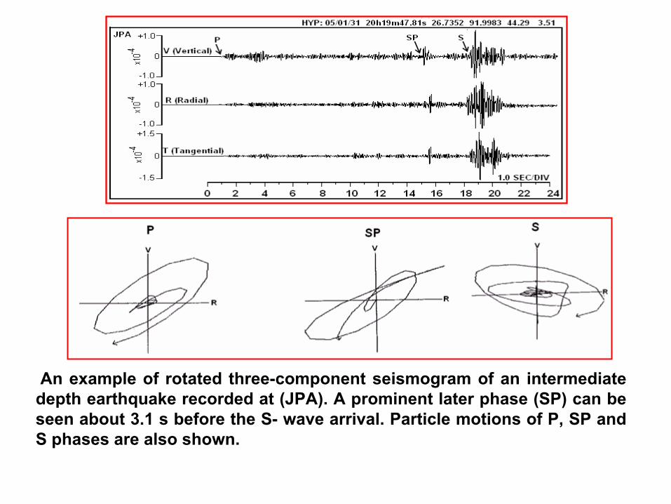
An example of rotated three-component seismogram of an intermediate depth earthquake recorded at (JPA). A prominent later phase (SP)
can be
seen about 3.1 s before the S-
wave arrival. Particle motions of P, SP and S phases are also shown.

Hm
(Φ΄, λ΄) = C0
+C1
Φ΄+C2
λ΄+C3
Φ΄2+C4
Φ΄
λ΄+ -------
+C14
λ΄4
Theoretical consideration
The reflected, refracted phases and converted phases (PS and SP) at Moho
are observed in seismograms for local earthquakes. Travel times
of these phases are inverted to estimate depth of the Moho
discontinuity. Depth distribution of the Moho
are expressed as a function of
latitude and longitude. The Moho
depth (Hm) at a location (Φ΄,λ΄
) is expressed as :
where Φ΄
and λ΄
are the latitude and longitude respectively. Ck
’s are unknown parameters which may be determined by inversion of the
observed travel time data.
-----(1)
Nakajima 2002

Travel time residuals can be written as :
eCCT
CTTT k
k
p
k
p
k
calpp
obspp +Δ
∂∂
−∂∂
=− ∑−− )( 121212
Where P1
and P2
denote the first and the later phases, respectively. For example,P1
and P2
are P and PmP
for the PmP- P data. ΔCk
is a correction term for unknown parameters and e is an error.
Partial derivatives of T are expressed as:
k
m
mk CH
HT
CT
∂∂
∂∂
=∂∂
Partial derivatives of Hm
against Ck
is calculated from equation (1)
-------------------
(2)
-------------------
(3)

1
2V
CosHT m θ∂=∂ ------
(4)
and we obtain
1
2V
CosHT
m
θ=
∂∂
The travel time change for the reflected wave due to change in depth of the interface as expressed by
---------
(5)
Fig (c)Similarly, we obtain the partial derivative ∂T/∂Hm
for the
converted wave as
2
2
1
1
VCos
VCos
HT
m
θθ−=
∂∂ --------
(6)
(A) Travel time change of reflected waves due to the depth change of the Moho
(B) Travel time change of converted waves due to the depth of the Moho.
Change in Travel times for reflected and converted
(A)
(B)

Eq. (2) can be expressed by matrix form as
d=G m +e -------------------------(7)
whered=the column vectors of residuals between observed and theoretical
travel time differenceG=matrix of partial derivativesm= column vector of correction term of unknown parameters ΔCKe=error vector
m=(GTG)-1GTd --------------------(8)
This equation can be written as follows by solving with least squares method:
This calculation is carried out iteratively until ΔCK
becomes sufficiently small.
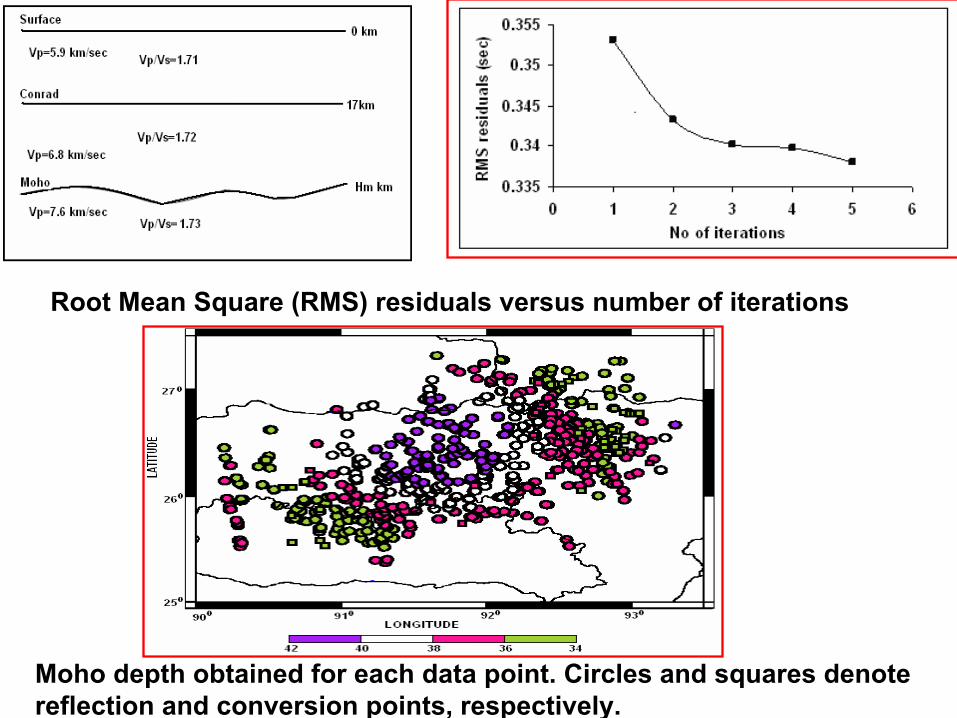
Root Mean Square (RMS) residuals versus number of iterations
Moho
depth obtained for each data point. Circles and squares denote reflection and conversion points, respectively.

Contour diagram represents the RMS residuals of each of the iteration.
Results

Depth distribution of Moho
obtained at the reflection and conversion points

STRESS ANALYSIS IN NORTHEASTERN INDIA AND ITS KINEMATICS IMPLICATIONS

SEISMIC STATIONS IN NE INDIA

WAVEFORM INVERSION OF19 AUGUST 2009 EVENT

MAP DISTRIBUTIONOF EPICENTERS OF 285 EARTHQUAKES
CONSIDERED IN THIS STUDY
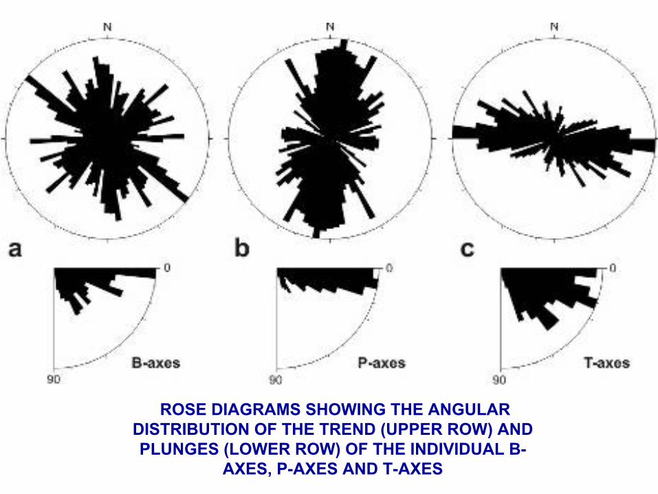
ROSE DIAGRAMS SHOWING THE ANGULAR DISTRIBUTION OF THE TREND (UPPER ROW) AND PLUNGES (LOWER ROW) OF THE INDIVIDUAL B-
AXES, P-AXES AND T-AXES

LARGE ARROWS SHOW INFERRED TREND OF COMPRESSION (CONVERGENT PAIRS OF ARROWS) AND EXTENSION (DIVERGENT ONES).
(A)WHOLE SET OF DATA, WITH 285 EARTHQUAKE FOCAL MECHANISMS.
(B) COMPRESSIVE SUBSET, INCLUDING 182 MECHANISMS.
(C) EXTENSIONAL SUBSET, INCLUDING 103 MECHANISMS

STEREOPLOTS SHOWING
THE DENSITY
DISTRIBUTION OFPRESSURE AND
TENSIONON THE SPHERE OR
ALL SPATIALLY
DEFINED SUBSETS
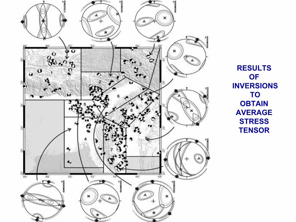
RESULTS OF
INVERSIONSTO
OBTAINAVERAGE STRESSTENSOR
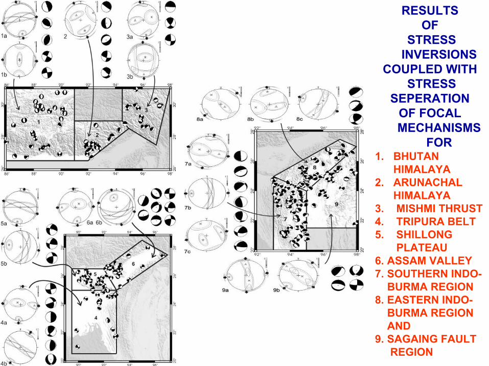
RESULTS OF
STRESS INVERSIONS
COUPLED WITHSTRESS
SEPERATIONOF FOCAL MECHANISMS
FOR1.
BHUTAN HIMALAYA
2.
ARUNACHAL HIMALAYA
3. MISHMI THRUST 4. TRIPURA BELT5. SHILLONG
PLATEAU6. ASSAM VALLEY7. SOUTHERN INDO-
BURMA REGION8. EASTERN INDO-
BURMA REGION AND
9. SAGAING FAULT REGION

SYNTHESIS OF MAIN STRESS REGIMES. PAIRS OF CONVERGENT ARROWS FOR COMPRESSION,
DIVERGENT ARROWS FOR EXTENSION.

Map of focal mechanism solutions in the Indo - Burma Ranges. The three maps correspond to différent Earthquake depth ranges in the same area: (a) 0-45 km (56) ; (b) 45-90 km (39) and (c) 90-160 km (38).

MAJOR KINEMATIC FEATURES OF
NORTHEAST INDIA.(a) PRESENT DAY
AVERAGE VELOCITIES RELATIVE TO LASHA,
TIBET: 1 WESTERN EDGE OF SUNDA
PLATE 2 CENTRAL MYANMAR BASINS
3 BENGAL BASIN4 SHILLONG-MIKIR
MASSIF. (b) TO THE EAST, VELOCITY OF 1
wrt. 2 (c) MAINLY ACCOMODATED
ALONG SAGAING FAULT, (d) TO THE
WEST, VELOCITY OF 2 wrt. 3 ACCOMODATED
ACROSS VARIOUS FAULTS OF BURMESE
ARC AND TRIPURA BELT
Geophys. J. Int. , 2009

CONCLUSION•
North-
South compression, in a direction consistent
with India-Eurasia convergence, prevails in the whole area from the Eastern Himalayas to the Bengal Basin through Shillong-Mikir
–Assam Valley block
and the Indian Craton.
•
The Indo-Burma ranges reveals complex stress pattern.
•
Indo-Burma ranges are under compression as a result of oblique convergence between the Sunda
and Indian plates. The maximum compressive stress rotates from NE-SW across the inner and northern arc to E-W near Bengal Basin.

ACKNOWLEDGEMENT
I SINCERELY CONVEY MY HEARTFELT THANKS TO
PROF. CATHERINE DORBATH
FOR INVITING ME to EOST
ALSO
THANKS TO THE ORGANIZER OF THE SEMINAR
