INTRODUCTION TO THE

MANY-BODY PROBLEM

UNIVERSITY OF FRIBOURG

SPRING TERM 2010

Dionys Baeriswyl

General literature

A. A. Abrikosov, L. P. Gorkov and I. E. Dzyaloshinski, Methods of Quantum

Field Theory in Statistical Physics, Prentice-Hall 1963.

A. L. Fetter and J. D. Walecka, Quantum Theory of Many-Particle Systems,McGraw-Hill 1971.

G. D. Mahan, Many-Particle Physics, Plenum Press 1981.

J. W. Negele and H. Orland, Quantum Many Particle Systems, Perseus Books1998.

Ph. A. Martin and F. Rothen, Many-Body Problems and Quantum Field Theory,Springer-Verlag 2002.

H. Bruus and K. Flensberg, Many-Body Quantum Theory in Condensed Matter

Physics, Oxford University Press 2004.

Contents

1 Second quantization 21.1 Many-particle states . . . . . . . . . . . . . . . . . . . . . . . . . 21.2 Fock space . . . . . . . . . . . . . . . . . . . . . . . . . . . . . . . 31.3 Creation and annihilation operators . . . . . . . . . . . . . . . . . 51.4 Quantum fields . . . . . . . . . . . . . . . . . . . . . . . . . . . . 71.5 Representation of observables . . . . . . . . . . . . . . . . . . . . 101.6 Wick’s theorem . . . . . . . . . . . . . . . . . . . . . . . . . . . . 16

2 Many-boson systems 192.1 Bose-Einstein condensation in a trap . . . . . . . . . . . . . . . . 192.2 The weakly interacting Bose gas . . . . . . . . . . . . . . . . . . . 202.3 The Gross-Pitaevskii equation . . . . . . . . . . . . . . . . . . . . 23

3 Many-electron systems 263.1 The jellium model . . . . . . . . . . . . . . . . . . . . . . . . . . . 263.2 Hartree-Fock approximation . . . . . . . . . . . . . . . . . . . . . 273.3 The Wigner crystal . . . . . . . . . . . . . . . . . . . . . . . . . . 283.4 The Hubbard model . . . . . . . . . . . . . . . . . . . . . . . . . 29

4 Magnetism 344.1 Exchange . . . . . . . . . . . . . . . . . . . . . . . . . . . . . . . 344.2 Magnetic order in the Heisenberg model . . . . . . . . . . . . . . 36

5 Electrons and phonons 395.1 The harmonic crystal . . . . . . . . . . . . . . . . . . . . . . . . . 395.2 Electron-phonon interaction . . . . . . . . . . . . . . . . . . . . . 415.3 Phonon-induced attraction . . . . . . . . . . . . . . . . . . . . . . 42

6 Superconductivity: BCS theory 446.1 Cooper pairs . . . . . . . . . . . . . . . . . . . . . . . . . . . . . . 446.2 BCS ground state . . . . . . . . . . . . . . . . . . . . . . . . . . . 456.3 Thermodynamics . . . . . . . . . . . . . . . . . . . . . . . . . . . 48

1

1 Second quantization

1.1 Many-particle states

Single-particle states are represented by vectors |ψ〉, |φ〉 of a Hilbert space H.Two-particle states are constructed in terms of the tensor product |φ〉 ⊗ |ψ〉, inshort |φ〉|ψ〉 with appropriate rules for addition, multiplication with a complexnumber and scalar product (see course on Quantum Mechanics). This construc-tion is readily extended to an arbitrary number of particles. We will be mostlyconcerned with identical particles, for which the Hamiltonian is invariant underany permutation. In order to define permutation operators we number the parti-cles according to the positions within the tensor product. Thus in the two-particlestate

|Ψ〉 = |ψ〉|φ〉 (1.1)

the particle number 1 is in the state |ψ〉, particle number 2 in state |φ〉. If thetwo single-particle states are different, the same holds for the states |Ψ〉 and

P12|Ψ〉 := |φ〉|ψ〉 . (1.2)

The permutation operator is both Hermitean and unitary, and therefore its eigen-values are ±1, with eigenstates 1√

2(|ψ〉|φ〉 ± |φ〉|ψ〉). The Hamiltonian H must

commute with P12 (see below), and therefore the eigenfunctions of H for twoidentical particles are either symmetric or antisymmetric.

Consider now three single-particle states |α〉, |β〉, |γ〉, which we assume to beorthonormal, 〈α|α〉 = 1, 〈α|β〉 = 0, and so on. The six permutation operatorsP12, P23, P31, P123, (P123)

2 and P 2ij = E (unity), where the cyclic permutation P123

acts as P123|α〉|β〉|γ〉 = |γ〉|α〉|β〉, are not mutually commutative, but there existfour invariant subspaces, two one-dimensional and two two-dimensional spaces.One one-dimensional subspace consists of the state

1√6

(|α〉|β〉|γ〉+ |β〉|α〉|γ〉+ |α〉|γ〉|β〉+ |γ〉|β〉|α〉+ |γ〉|α〉|β〉+ |β〉|γ〉|α〉) ,

which is symmetric under all permutation operators, the other one consists of thefully anti-symmetric state

1√6

(|α〉|β〉|γ〉 − |β〉|α〉|γ〉 − |α〉|γ〉|β〉 − |γ〉|β〉|α〉+ |γ〉|α〉|β〉+ |β〉|γ〉|α〉) ,

which changes sign for the odd permutations P12, P23, P31 and is invariant underthe even permutations P123, (P123)

2. (A permutation is even if it is obtained byan even number of pair interchanges, otherwise it is odd.) The two states

1√12

(2|α〉|β〉|γ〉+ 2|β〉|α〉|γ〉 − |α〉|γ〉|β〉 − |γ〉|β〉|α〉 − |γ〉|α〉|β〉 − |β〉|γ〉|α〉) ,

1

2(−|α〉|γ〉|β〉+ |γ〉|β〉|α〉+ |γ〉|α〉|β〉 − |β〉|γ〉|α〉) ,

2

transform into a linear combination of each other under the action of the permu-tation operators, and the same holds for the remaining two states

1

2(−|α〉|γ〉|β〉 + |γ〉|β〉|α〉 − |γ〉|α〉|β〉+ |β〉|γ〉|α〉) ,

1√12

(2|α〉|β〉|γ〉 − 2|β〉|α〉|γ〉+ |α〉|γ〉|β〉+ |γ〉|β〉|α〉 − |γ〉|α〉|β〉 − |β〉|γ〉|α〉) .

We apply the principle of indistinguishability (A. M. L. Messiah and O. W. Green-berg, Phys. Rev. 136, B248 (1964)), according to which two states that differ onlyby a permutation of identical particles cannot be distinguished by any observa-tion. This means that

〈Ψ|A|Ψ〉 = 〈Ψ|PijAPij|Ψ〉 (1.3)

for an arbitrary observable A and an arbitrary state |Ψ〉. Therefore

[A,Pij] = 0 , (1.4)

i.e., any observable A commutes with any permutation operator.The six permutation operators form a group, and their action on the states

given above can be used for constructing irreducible representations of this group.There are two one-dimensional and one two-dimensional irreducible representa-tions. Group theory is also useful for characterizing the eigenstates of any Hamil-tonian which is invariant under permutations. It implies that matrix elementsvanish between states belonging to different irreducible representations. Thesetherefore can be used to label the energy eigenvalues, while their dimension isequal to the degeneracy of eigenvalues (if there are no accidental degeneracies).

It is an empirical fact that only fully symmetric or antisymmetric states arerealized. Moreover, as proven in quantum field theory, particles with integer spinhave only symmetric states (these particles are called bosons), whereas particleswith half odd-integer spin have only antisymmetric states (these particles arecalled fermions). Antisymmetric states vanish if two single-particle states areidentical. This is just the Pauli principle, according to which two fermions cannotoccupy the same single-particle state.

1.2 Fock space

Often there exists a natural basis of single-particles states, for instance the statesrelated to the energy levels of an atom or the Bloch states for a particle ina periodic potential. Let {|φi〉} be an orthonormal basis of the single-particleHilbert space, 〈φi|φj〉 = δi,j . A basis for fully symmetric and anti-symmetricN -particle states is then given by

|Ψ〉± = N±∑

p

(1

sign p

)

|χp1〉|χp2〉...|χpN〉 , (1.5)

where χj ∈ {|φi〉} are (not necessarily distinct) single-particle states, N± is a nor-

malization factor, the sum runs over all N ! permutations p =

(1 2 ... Np1 p2 ... pN

)

3

and sign p = +1 for permutations corresponding to an even number of transpo-sitions and sign p = −1 otherwise. Instead of specifying the states (1.5) by allthe single-particle states it is more convenient to indicate the number of timesa single-particle state appears. Let us call ni the number of times the state |φi〉appears in the product |χ1〉|χ2〉...|χN〉. This number ni is the occupation number

of the state |φi〉. Then the state (1.5) can be specified as

|Ψ〉± = |n1, n2, . . .〉± , (1.6)

where there are n1 particles in |φ1〉, n2 particles in |φ2〉 and so forth. For bosonsni = 0, 1, 2, 3, . . ., and for fermions ni = 0, 1, according to the Pauli principle. Foran N -particle state we have the restriction

∑

i ni = N .Two states |n1, n2, ...〉, |n′

1, n′2, ...〉 are orthogonal if they differ in at least one

occupation number, i.e. ni 6= n′i for some number i. If all the occupation numbers

coincide, we find〈Ψ±|Ψ±〉 = N2

± N ! n1! n2!... (1.7)

Thus the normalization factor is N± = 1/√N ! n1! n2! ..., and we get

〈n′1, n

′2, ...|n1, n2, ...〉 = δn1,n′

1δn2,n′

2... (1.8)

It is important to realize that the occupation number representation (1.6) dependson the single-particle basis. In general one tries to make a judicious choice dic-tated by the physical problem at hand. To keep the notation simple we drop thesubscript ± in (1.6). But one has to remember that the states in the occupationnumber representation are symmetric for bosons and antisymmetric for fermions.

The states |n1, n2, ...〉 form an orthonormal basis of the N -particle Hilbertspace HN

± . Thus any state of HN± can be written as a linear combination

|Ψ〉 =∑

n1,n2,...P

ni=N

c(n1, n2, . . .)|n1, n2, . . .〉 . (1.9)

If we remove the restriction∑ni = N we obtain a linear combination of states

where the number of particles is not specified,

|Ψ〉 =∑

n1,n2,...

c(n1, n2, . . .)|n1, n2, . . .〉 . (1.10)

Two Hilbert spaces with different particle numbers have no state vector in com-mon. Thus states of the form (1.9) belong to the Hilbert space formed by thedirect sum ∞⊕

N=0

HN± = F± .

In this expression H0± consists of the vacuum state |0, 0, 0, . . .〉. The space F± is

called Fock space. It consists of symmetric (bosons) resp. antisymmetric (fermions)state vectors, the number of particles being unspecified. F± is the appropriateHilbert space for the formalism of second quantization.

4

1.3 Creation and annihilation operators

“Second quantization” does not mean that we quantize the theory once more, itmerely provides an elegant formalism for dealing with many-fermion and many-boson systems. Formally, as will be shown later, the transition from the quantumtheory for a single particle to a many-body theory can be made by replacing thewave functions by field operators. For electromagnetic fields this procedure wouldindeed correspond to a true quantization, but not in the present context.

a) Bosons

The creation operator a†i and annihilation operator ai of a boson in the state |φi〉are defined by

a†i |n1, n2, . . . , ni, . . .〉 =√ni + 1 |n1, n2, . . . , ni + 1, . . .〉 ,

ai|n1, n2, . . . , ni, . . .〉 =√ni |n1, n2, . . . , ni − 1, . . .〉 . (1.11)

In addition to these two relations we require these operators to be linear. In thisway the creation and annihilation operators are completely specified. Relation(1.8) implies that the only non zero matrix elements of ai are

〈n1, n2, . . . , ni − 1, . . . |ai|n1, n2, . . . , ni, . . .〉 =√ni . (1.12)

The only non zero matrix elements of a†i are

〈n1, n2, . . . , ni, . . . |a†i |n1, n2, . . . , ni − 1, . . .〉 = (ni − 1 + 1)12 = (ni)

12 . (1.13)

Formulae (1.12) and (1.13) show that a†i is the adjoint of ai. Eq. (1.11) allows toprove the algebraic relations

[ai, a†j] = aia

†j − a†jai = δij ,

[ai, aj] = [a†i , a†j ] = 0 . (1.14)

For i = j the algebra is the same as that for the raising and lowering operatorsof the harmonic oscillator. Operators for different single-particle states |φi〉 and|φj〉 commute. To prove the first relation for i = j we act with the operators aia

†i

and a†iai on a general state in Fock space,

aia†i |..., ni, ...〉 =

√ni + 1 ai|..., ni + 1, ...〉 = (ni + 1)|..., ni, ...〉 ,

a†iai|..., ni, ...〉 =√ni a

†i |..., ni − 1, ...〉 = ni|..., ni, ...〉 .

Substracting the two relations we find [ai, a†i ]|..., ni, ...〉 = |..., ni, ...〉 for an arbi-

trary basis state, which proves the first relation in (1.14) for i = j. The otherrelations are demonstrated in the same way.

b) Fermions

The creation and annihilation operators, defined by

a†i |n1, n2, . . . , ni, . . .〉 = (1 − ni)(−1)ǫi|n1, n2, . . . , ni + 1, . . .〉 ,ai|n1, n2, . . . , ni, . . .〉 = ni(−1)ǫi|n1, n2, . . . , ni − 1, . . .〉 , (1.15)

5

take into account the fermionic sign through the number of transpositions in-volved, ǫi =

∑i−1s=1 ns. If state |φi〉 is already occupied (ni = 1), then we have

a†i |n1, n2, ..., 1, ...〉 = 0, in agreement with the Pauli principle. As in the bosoniccase one shows easily that a†i is the adjoint of ai. These operators satisfy thealgebra

{ai, a†j} := aia

†j + a†jai = δij ,

{ai, aj} = {a†i , a†j} = 0 . (1.16)

In particular a2i = (a†i)

2 = 0, which is again an expression of the Pauli principle.The anticommutation relations for fermions (1.16) are proven in the same way asthe commutation relations (1.14) for bosons.

c) Number operator

Eqs. (1.11) (1.15) imply for both Bose and Fermi statistics

a†iai| . . . , ni, . . .〉 = ni| . . . , ni, . . .〉 . (1.17)

Thus the operator a†iai counts the number of particles in the state |φi〉, and thetotal number of particles is measured by the operator

N =

∞∑

i=1

a†iai . (1.18)

We have

N |n1, n2, n3, . . .〉 =

∞∑

i=1

ni|n1, n2, n3, . . .〉 . (1.19)

d) Construction of states out of the vacuum

The vacuum state, corresponding to n1 = 0, n2 = 0, . . ., is denoted by |0〉. Actingon |0〉 with products (or polynomials) of a†i and aj yields states in Fock space.

Using the definitions of a†i and aj one shows that

|n1, n2, . . . , ni, . . .〉 =(a†1)

n1

√n1!

(a†2)n2

√n2!

· · · (a†i )

ni

√ni!

· · · |0〉 . (1.20)

The Fock space is spanned by the states |n1, n2, . . . , ni, . . .〉. Therefore an ar-bitrary state can be obtained by acting on |0〉 by some polynomial of creationoperators a†i .

To illustrate the formalism, we consider a few simple examples.

(1) As a first example we consider an atom where the single-particle statescorrespond to energy levels. With the operation (1.20), specified energylevels are occupied, for instance in

a†1a†4|0〉 = |1, 0, 0, 1, 0, 0, . . .〉

the operator a†4 puts an electron into level 4, subsequently the operator a†1puts a second electron into level 1.

6

(2) The Fermi sea for free electrons can be written as

|F〉 =∏

k, |k|<kF

σ=↑,↓

a†kσ|0〉 ,

where a†kσ creates an electron with momentum ~k and spin projection σ.

(3) The Bardeen-Cooper-Schrieffer state is given by

|BCS〉 =∏

k

(uk + vka†k↑a

†−k↓)|0〉, |uk|2 + |vk|2 = 1 ,

where a†k↑ a†−k↓ creates a Cooper pair. Notice that this state is not an

eigenstate of the particle number operator.

(4) Finally, a Bose condensate for N free bosons corresponds to

(a†k=0)N

√N !

|0〉 .

1.4 Quantum fields

For many applications the coordinate representation turns out to be useful. Weintroduce the family of operators Ψ†(r) through the relation

Ψ†(r)|0〉 := |r〉. (1.21)

Thus Ψ†(r) creates a particle at r. (Depending on the situation, one has also tospecify some other quantum numbers, for instance the spin of an electron; in thiscase we will use the notation Ψ†

σ(r).) Using the completeness of single-particlestates |φi〉, we arrive at

Ψ†(r)|0〉 =∑

i

〈φi|r〉|φi〉 =∑

i

φ∗i (r) a

†i |0〉. (1.22)

Thus the operator Ψ†(r) and the adjoint operator Ψ(r) can also be defined withrespect to a given basis,

Ψ†(r) =∑

i

φ∗i (r) a

†i ,

Ψ(r) =∑

i

φi(r) ai . (1.23)

These operators are also called quantum fields. To obtain their properties, we willuse extensively the closure and orthonormality relations for the single-particlewave functions

∑

i

φ∗i (r)φi(r

′) = δ(r − r′) ,

∫

d3r φ∗i (r)φj(r) = δij . (1.24)

7

a) Spinless bosons

The commutation relations for the field operators of (spin zero) bosons are readilyfound using the definition (1.23) together with the closure relation of Eq. (1.24),

[Ψ(r),Ψ†(r′)] = δ(r − r′) ,

[Ψ(r),Ψ(r′)] = [Ψ†(r),Ψ†(r′)] = 0 . (1.25)

The particle number operator (1.18) can be expressed by the field operators (1.23),using the orthogonality relation of Eq. (1.24),

N =

∫

d3rΨ†(r)Ψ(r) . (1.26)

Thus Ψ†(r)Ψ(r) can be interpreted as the density of particles at r. This inter-pretation reminds us of the probability density for a particle in state ψ(r) to beat r, and it suggests that the transition from single-particle quantum mechanicsto many-body theory is accomplished be replacing the wave function ψ(r) bythe operator Ψ(r). The same rule will be found for other single-particle observ-ables. From this point of view the expression “second quantization”, althoughmisleading, makes sense.

b) Fermions

For spin 12

fermions we have to include the spin degrees of freedom labeled byσ =↑, ↓,

ai → aiσ, Ψ(r) → Ψσ(r) . (1.27)

Thus we treat the spin as an additional quantum number and do not write downexplicitly the two-dimensional column vectors representing the spin states. Theanticommutation relations (1.16) are replaced by

{aiσ, a†jσ′} = δijδσσ′ ,

{aiσ, ajσ′} = {a†iσ, a†jσ′} = 0 . (1.28)

Correspondingly, the field operators

Ψσ(r) :=∑

i

φi(r) aiσ (1.29)

satisfy the anticommutation relations

{Ψσ(r),Ψ†σ′(r

′)} = δ(r− r′)δσσ′ ,

{Ψσ(r),Ψσ′(r′)} = {Ψ†σ(r),Ψ

†σ′(r

′)} = 0 . (1.30)

The number operator is given by

N =∑

σ

∫

d3rΨ†σ(r)Ψσ(r) . (1.31)

and therefore Ψ†σ(r)Ψσ(r) is the density of particles with spin σ at r.

8

To be specific we consider electrons in a cubic box of size V = L3 and applyperiodic boundary conditions. A natural basis is given by the plane waves

φk(r) = 〈r|k〉 =eik·r

V12

, (1.32)

where k = 2πLn, n = (nx, ny, nz) ∈ Z

3. The creation and annihilation operators

of an electron with wave vector k and spin σ ∈ {↑, ↓} are a†kσ and akσ. The fieldoperators of the electrons are therefore given by the Fourier transforms

Ψ†σ(r) =

1

V12

∑

k

e−ik·ra†kσ ,

Ψσ(r) =1

V12

∑

k

eik·rakσ . (1.33)

The density at point r is determined by the operator

n(r) = Ψ†↑(r)Ψ↑(r) + Ψ†

↓(r)Ψ↓(r) (1.34)

and the total electron number operator is

N =∑

σ=↑,↓

∫

V

d3rΨ†σ(r)Ψσ(r) =

∑

k,σ

a†kσakσ . (1.35)

c) Many-particle wave functions

In the same way as many-particle states can be constructed by applying productsof creation operators a†i , defined with respect to a single-particle basis {|φi〉}, tothe vacuum state |0〉, we can generate states

|r1, r2, . . . , rN〉 := Ψ†(r1)Ψ†(r2) . . .Ψ

†(rN)|0〉 , (1.36)

or, for particles with non-zero spin,

|r1σ1, r2σ2, . . . , rNσN〉 := Ψ†σ1

(r1)Ψ†σ2

(r2) . . .Ψ†σN

(rN)|0〉 . (1.37)

These are states where the N particles sit at the sites r1, r2, . . . , rN (possibly withspins σ1, σ2, . . . , σN ). They can be used for setting up a coordinate representationfor any N -particle state.

Consider for example the particular state of N spin 12

fermions

|1τ1, 2τ2, . . . , NτN 〉 := a†1τ1a†2τ2

. . . a†NτN|0〉 , (1.38)

where a†iτicreates a particle in the state |φi〉 with spin τi = ↑ or ↓. The bra

corresponding to the ket (1.37) is

〈r1σ1, r2σ2, . . . , rNσN | = 〈0|ΨσN(rN) · · ·Ψσ2(r2)Ψσ1(r1) . (1.39)

Therefore, using Eq. (1.29), we find the coordinate representation

〈r1σ1, r2σ2, . . . , rNσN |1τ1, 2τ2, . . . , NτN 〉=

∑

i1,...,iN

φi1(r1) · · ·φiN (rN) 〈0|aiNσN· · ·ai1σ1a

†1τ1

· · ·a†NτN|0〉 . (1.40)

9

The matrix element 〈0|aiN σN· · ·ai1σ1a

†1τ1 · · ·a

†NτN

|0〉 is non-zero only if the se-quence (i1, i2, ..., iN) is a permutation p of (1, 2, ..., N). In this case one obtains(Wick’s theorem, to be discussed later)

〈0|aiNσN· · ·ai1σ1a

†1τ1 · · ·a

†NτN

|0〉 = sign p δσ1,τp1· · · δσN ,τpN

. (1.41)

The many-body wave function representing the state |1τ1, 2τ2, . . . , NτN 〉 is there-fore given by

〈r1σ1, ..., rNσN |1τ1, ..., NτN〉 =∑

p

sign p φp1(r1)δσ1,τp1· · ·φpN

(rN)δσN ,τpN,

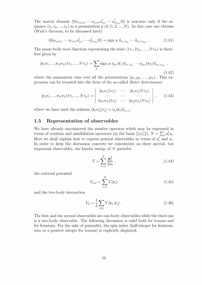
(1.42)where the summation runs over all the permutations (p1, p2, . . . , pN). This ex-pression can be recasted into the form of the so-called Slater determinant

〈r1σ1, ..., rNσN |1τ1, ..., NτN 〉 =

∣∣∣∣∣∣

〈r1σ1|1τ1〉 · · · 〈r1σ1|NτN 〉· · · · · · · · ·

〈rNσN |1τ1〉 · · · 〈rNσN |NτN 〉

∣∣∣∣∣∣

, (1.43)

where we have used the relation 〈riσi|jτj〉 = φj(ri)δσi,τj.

1.5 Representation of observables

We have already encountered the number operator which may be expressed interms of creation and annihilation operators (in the basis {|φi〉}), N =

∑

i a†iai.

Here we shall explain how to express general observables in terms of a†i and ai.In order to keep the discussion concrete we concentrate on three special, butimportant observables, the kinetic energy of N particles

T =N∑

i=1

p2i

2m, (1.44)

the external potential

Vext =

N∑

i=1

U(ri) (1.45)

and the two-body interaction

V2 =1

2

∑

i6=j

V (ri, rj) . (1.46)

The first and the second observables are one-body observables while the third oneis a two-body observable. The following discussion is valid both for bosons andfor fermions. For the sake of generality, the spin index (half-integer for fermions,zero or a positive integer for bosons) is explicitly displayed.

10

a) Kinetic energy

We start with the kinetic energy T which is diagonal in the basis of plane waves|k, σ〉. Thus we have

T |k1σ1,k2σ2, ...,kNσN 〉 =

N∑

i=1

(~

2k2i

2m

)

|k1σ1,k2σ2, ...,kNσN〉 . (1.47)

In second-quantized form the N -particle state is written as

|k1σ1,k2σ2, ...,kNσN 〉 = a†k1σ1a†k2σ2

...a†kN σN|0〉 . (1.48)

The number of particles in the state |k, σ〉 is a†kσakσ, so we expect

T =∑

k,σ

|~k|22m

a†kσakσ . (1.49)

In order to prove this statement we have to show that the application of thisoperator onto any N -particle state (1.48) reproduces Eq. (1.47). The followingalgebraic relation will be useful,

[

a†kσakσ, a†kiσi

]

= a†kiσiδk,ki

δσ,σi. (1.50)

It holds both for bosons and fermions. Applying this relation step by step, i.e.

a†kσakσa†k1σ1

a†k2σ2...a†kN σN

|0〉 =[

a†kσakσ, a†k1σ1

]

a†k2σ2...a†kN σN

|0〉 + a†k1σ1a†kσakσa

†k2σ2

...a†kN σN|0〉 , (1.51)

we finda†kσakσa

†k1σ1

a†k2σ2...a†kN σN

|0〉 = nkσa†k1σ1

a†k2σ2...a†kN σN

|0〉 , (1.52)

where nkσ is the number of times the quantum number kσ appears in the state|k1σ1,k2σ2, ...,kNσN〉. It is now obvious that Eq. (1.47) is fulfilled and thereforethe kinetic energy is indeed given by Eq. (1.49).

Expression (1.49) is simple and intuitive because the underlying basis diago-nalises the kinetic energy. It is useful to have T in coordinate basis. Inverting(1.33),

a†kσ =1

V12

∫

V

d3r eik·rΨ†σ(r) ,

akσ =1

V12

∫

V

d3r e−ik·rΨσ(r) , (1.53)

we obtain

k2a†kσakσ =1

V

∫

V

d3rΨ†σ(r)∇eik·r ·

∫

V

d3r′ Ψσ(r′)∇′e−ik′·r′

=1

V

∫

V

d3r eik·r∇Ψ†σ(r) ·

∫

V

d3r′ e−ik′·r′∇′Ψσ(r′) , (1.54)

11

where we have used partial integration together with periodic boundary condi-tions (V = L3, kα = 2πνα/L, α = x, y, z). Using the relation 1

1

V

∑

k

eik·(r−r′) = δ(r − r′) (1.55)

we get

T =~

2

2m

∑

σ

∫

V

d3r∇Ψ†σ(r) · ∇Ψσ(r) , (1.56)

where the gradient operator acts only on the immediately following field operator.

b) External potential

The one-body potential Vext is diagonal in coordinate space,

Vext|r1σ1, ..., rN , σN〉 =

(N∑

i=1

U(ri)

)

|r1σ1, ..., rNσN 〉 , (1.57)

where in the state |r1σ1, ..., rN , σN〉 one particle is at r1 with spin σ1, one at r2

with spin σ2, and so on, i.e.

|r1σ1, ..., rNσN〉 = Ψ†σ1

(r1)...Ψ†σN

(rN)|0〉 . (1.58)

We claim now that the second-quantized representation of the external potentialis given by

Vext =∑

σ

∫

d3rU(r)Ψ†σ(r)Ψσ(r) =

∫

d3rU(r)n(r) . (1.59)

The proof proceeds as above for the kinetic energy. We notice that the commu-tation relation

[Ψ†

σ(r)Ψσ(r),Ψ†σi

(ri)]

= δσ,σiδ(r − ri)Ψ

†σi

(ri) (1.60)

holds both for bosons and fermions. Applying the operator (1.59) to the right-hand side of (1.58), we find indeed

(∑

σ

∫

d3r U(r)Ψ†σ(r)Ψσ(r)

)

Ψ†σ1

(r1)...Ψ†σN

(rN)|0〉

=

(N∑

i=1

U(ri)

)

Ψ†σ1

(r1)...Ψ†σN

(rN)|0〉 . (1.61)

The momentum representation of the external potential is easily obtained usingEq. (1.33),

Vext =∑

σ

∫

d3r U(r)1

V

∑

k,k′

e−i(k−k′)·ra†k,σak′,σ

=1

V

∑

k,k′,σ

U(k − k′)a†k,σak′,σ , (1.62)

1In the theory of generalized functions one shows the relation∑

∞

n=−∞δ(x − nL) =

1

L

∑∞

ν=−∞e2πiνx/L. If x is limited to an interval of length L only one term of the l.h.s. survives.

12

k,s k'=k+q,s

U(q)^

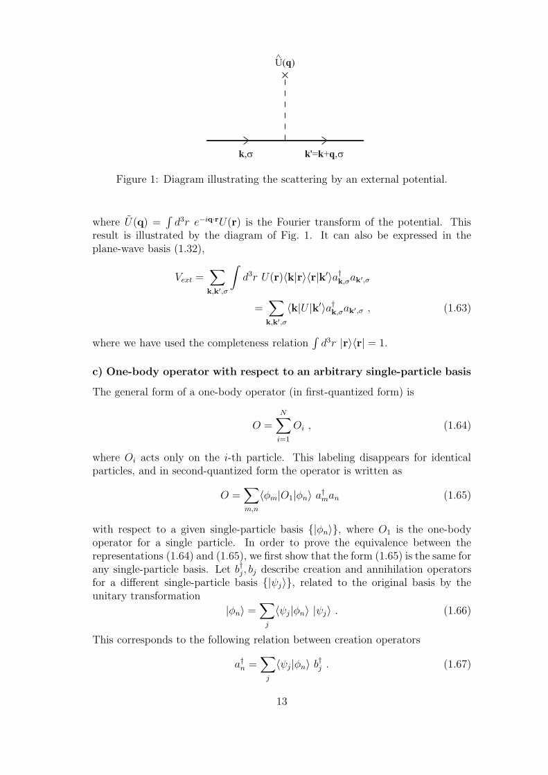
Figure 1: Diagram illustrating the scattering by an external potential.

where U(q) =∫d3r e−iq·rU(r) is the Fourier transform of the potential. This

result is illustrated by the diagram of Fig. 1. It can also be expressed in theplane-wave basis (1.32),

Vext =∑

k,k′,σ

∫

d3r U(r)〈k|r〉〈r|k′〉a†k,σak′,σ

=∑

k,k′,σ

〈k|U |k′〉a†k,σak′,σ , (1.63)

where we have used the completeness relation∫d3r |r〉〈r| = 1.

c) One-body operator with respect to an arbitrary single-particle basis

The general form of a one-body operator (in first-quantized form) is

O =

N∑

i=1

Oi , (1.64)

where Oi acts only on the i-th particle. This labeling disappears for identicalparticles, and in second-quantized form the operator is written as

O =∑

m,n

〈φm|O1|φn〉 a†man (1.65)

with respect to a given single-particle basis {|φn〉}, where O1 is the one-bodyoperator for a single particle. In order to prove the equivalence between therepresentations (1.64) and (1.65), we first show that the form (1.65) is the same forany single-particle basis. Let b†j , bj describe creation and annihilation operatorsfor a different single-particle basis {|ψj〉}, related to the original basis by theunitary transformation

|φn〉 =∑

j

〈ψj|φn〉 |ψj〉 . (1.66)

This corresponds to the following relation between creation operators

a†n =∑

j

〈ψj|φn〉 b†j . (1.67)

13

The relation (1.33) between field operators Ψ†σ(r) and the creation operators a†k,σ

is a special example of such a transformation. Inserting Eqs. (1.66) and (1.67) intothe representation (1.65) and using the completeness relation

∑

n |φn〉〈φn| = 1,we readily find

O =∑

j,j′

〈ψj |O1|ψj′〉 b†jbj′ , (1.68)

i.e. indeed the same form as before. We can therefore choose any basis which isconvenient for demonstrating the equivalence between the representations (1.64)and (1.65). The obvious choice is a basis consisting of eigenvectors |χl〉 of O1,O1|χl〉 = ωl|χl〉. This yields the diagonal representation O =

∑

l ωlc†l cl in terms of

the corresponding creation and annihilation operators. The proof for the equiv-alence between the representations (1.64) and (1.65) proceeds then in the sameway as in the case of the kinetic energy.

d) Two-body operators

We will concentrate on a spin-independent two-body interaction as in Eq. (1.46)and proceed as in the case of Vext. The operator V2 is diagonal in coordinatespace,

V2|r1σ1, . . . , rNσN 〉 =

(

1

2

∑

i6=j

V2(ri, rj)

)

|r1σ1, . . . , rNσN〉 . (1.69)

It will be shown below that the second-quantized expression is

V2 =1

2

∑

σ,σ′

∫

d3r

∫

d3r′ V2(r, r′)Ψ†

σ(r)Ψ†σ′(r

′)Ψσ′(r′)Ψσ(r) . (1.70)

Often this expression is rewritten in terms of the density n(r),

V2 =1

2

∫

d3r

∫

d3r′ V2(r, r′) : n(r)n(r′) : . (1.71)

This formula is quite familiar except that the operators are normal ordered. Nor-mal order means that all the creation operators are put on the left of the anni-hilation operators and that for fermions one has to take into account the sign ofthe permutation involved in the rearrangement of the operators.

To show the equivalence of the first- and second-quantized representations, weverify that the application of Eq. (1.70) to a state |r1σ1, . . . , rNσN〉 reproducesEq. (1.69). To this end we use the relation

[

Ψ†σ(r)Ψ†

σ′(r′)Ψσ′(r′)Ψσ(r),Ψ†σi

(ri)]

= Ψ†σi

(ri)(

δσ,σiδr,ri

Ψ†σ′(r′)Ψσ′(r′) + δσ′,σi

δr′,riΨ†

σ(r)Ψσ(r))

, (1.72)

which is easily proven for both bosons and fermions. We use this relation to movethe field operators in Eq. (1.70) through the operators in the state (1.58)

Ψ†σ(r)Ψ†

σ′(r′)Ψσ′(r′)Ψσ(r)Ψ

†σ1

(r1) · · ·Ψ†σN

(rN)|0〉

=N∑

i=1

Ψ†σ1

(r1) · · ·[

Ψ†σ(r)Ψ

†σ′(r

′)Ψσ′(r′)Ψσ(r),Ψ†σi

(ri)]

· · ·Ψ†σN

(rN)|0〉. (1.73)

14

This implies

1

2

∑

σ,σ′

∫

d3r

∫

d3r′ V2(r, r′)Ψ†

σ(r)Ψ†σ′(r

′)Ψσ′(r′)Ψσ(r)|r1σ1, . . . , rNσN〉

=

N∑

i=1

Ψ†σ1

(r1) · · ·Ψ†σi

(ri)

∫

d3r V2(ri, r)n(r)Ψ†σi+1

(ri+1) · · ·Ψ†σN

(rN)|0〉 , (1.74)

where n(r) =∑

σ Ψ†σ(r)Ψσ(r), and we have used the symmetry V (r, r′) = V (r′, r).

We thus arrive at the problem of applying external potentials on many-particlestates, and we can use Eq. (1.61). This gives the desired result,

1

2

∑

σ,σ′

∫

d3r

∫

d3r′ V2(r, r′)Ψ†

σ(r)Ψ†σ′(r

′)Ψσ′(r′)Ψσ(r)|r1σ1, . . . , rNσN〉

=∑

i,ji>j

V2(ri, rj)|r1σ1, . . . , rNσN 〉 . (1.75)

The momentum space representation for the two-body interaction (1.70) is ob-tained by inserting the relation (1.33) for the quantum fields. One finds

V2 =1

2

∑

σ,σ′

∑

k1,k2,k3,k4

〈k1,k2|V2|k4,k3〉 a†k1,σa†k2,σ′ak3,σ′ak4,σ (1.76)

with matrix elements

〈k1,k2|V2|k4,k3〉 =1

V 2

∫

d3r

∫

d3r′ e−i(k1−k4)·re−i(k2−k3)·r′V2(r, r′) . (1.77)

For a homogeneous system the interaction depends only on the difference r − r′,V2(r, r

′) = V2(r−r′). Moreover, assuming periodic boundary conditions for V2(r),we have the Fourier series

V2(r) =1

V

∑

q

eiq·r V2(q) (1.78)

with q = 2πL

(ν1, ν2, ν3), νi ∈ Z. The matrix elements are then simplified asfollows,

〈k1,k2|V2|k4,k3〉 =1

VV2(q) δq,k1−k4 δq,−k2+k3 . (1.79)

With k1 = k, k2 = k′, k3 = k′ + q and k4 = k − q, the two-particle interactionbecomes

V2 =1

2V

∑

k,k′,qσ,σ′

V2(q) a†k,σa†k′,σ′ak′+q,σ′ak−q,σ . (1.80)

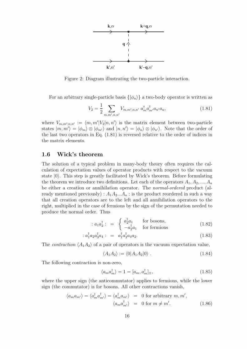
It can be viewed as a scattering process, where two particles with initial momenta~k and ~k′ interact and go out with final momenta ~(k − q) and ~(k′ + q) asillustrated in Fig. 2. Thereby the total momentum is conserved.

15

k',s' k'-q,s'

q

k,s k+q,s

Figure 2: Diagram illustrating the two-particle interaction.

For an arbitrary single-particle basis {|φn〉} a two-body operator is written as

V2 =1

2

∑

m,m′,n,n′

Vm,m′;n,n′ a†ma†m′an′an, (1.81)

where Vm,m′;n,n′ := 〈m,m′|V2|n, n′〉 is the matrix element between two-particlestates |m,m′〉 = |φm〉 ⊗ |φm′〉 and |n, n′〉 = |φn〉 ⊗ |φn′〉. Note that the order ofthe last two operators in Eq. (1.81) is reversed relative to the order of indices inthe matrix elements.

1.6 Wick’s theorem

The solution of a typical problem in many-body theory often requires the cal-culation of expectation values of operator products with respect to the vacuumstate |0〉. This step is greatly facilitated by Wick’s theorem. Before formulatingthe theorem we introduce two definitions. Let each of the operators A1, A2, ..., An

be either a creation or annihilation operator. The normal-ordered product (al-ready mentioned previously) : A1A2...An : is the product reordered in such a waythat all creation operators are to the left and all annihilation operators to theright, multiplied in the case of fermions by the sign of the permutation needed toproduce the normal order. Thus

: a1a†2 : =

{a†2a1 for bosons,

−a†2a1 for fermions(1.82)

: a†1a2a†3a4 : = a†1a

†3a4a2. (1.83)

The contraction 〈A1A2〉 of a pair of operators is the vacuum expectation value,

〈A1A2〉 := 〈0|A1A2|0〉 . (1.84)

The following contraction is non-zero,

〈ama†m〉 = 1 = [am, a

†m]±, (1.85)

where the upper sign (the anticommutator) applies to fermions, while the lowersign (the commutator) is for bosons. All other contractions vanish,

〈amam′〉 = 〈a†ma†m′〉 = 〈a†mam′〉 = 0 for arbitrary m,m′,

〈ama†m′〉 = 0 for m 6= m′. (1.86)

16

We can now state Wick’s theorem:

An ordinary product of any finite number of creation and annihilation oper-ators is equal to the sum of normal products from which 0,1,2,... contractionshave been removed in all possible ways.

For n = 2 this means:

A1A2 = : A1A2 : +〈A1A2〉. (1.87)

This is clearly true if both operators are creation operators or if both are annihila-tion operators. It also applies if A1 is a creation operator and A2 an annihilationoperator. In the remaining case where A1 = a1 and A2 = a†2 we can write theproduct as

a1a†2 = ∓a†2a1 + [a1, a

†2]±. (1.88)

In view of Eqs. (1.82) and (1.85) this is identical to Eq. (1.87). Wick’s theoremis therefore proven for n = 2. For n = 4 it asserts

A1A2A3A4 = : A1A2A3A4 :

+ : A1A2 : 〈A3A4〉 ∓ : A1A3 : 〈A2A4〉+ : A2A3 : 〈A1A4〉+ : A1A4 : 〈A2A3〉 ∓ : A2A4 : 〈A1A3〉+ : A3A4 : 〈A1A2〉+ 〈A1A2〉〈A3A4〉 ∓ 〈A1A3〉〈A2A4〉 + 〈A1A4〉〈A2A3〉 , (1.89)

where the upper sign refers to fermions, the lower to bosons.The following relation is very useful for proving Wick’s theorem:

: A1 · · ·An : B =

n∑

m=1

(∓)s〈AmB〉 : A1A2 · · ·Am−1Am+1 · · ·An :

+ : A1 · · ·AnB : , (1.90)

where s counts the number of pairwise permutations that are necessary to realizethe indicated sequence of operators. This relation is trivially fulfilled if B is anannihilation operator. If B is a creation operator, the contraction 〈AmB〉 vanishesif Am is also a creation operator, and therefore we can limit ourselves to the casewhere all Ai, i = 1 . . . n, are annihilation operators, i.e. we have to prove therelation

A1 · · ·AnB =n∑

m=1

(∓)s〈AmB〉A1A2 · · ·Am−1Am+1 · · ·An

+ (∓1)nBA1 · · ·An . (1.91)

We do this by induction. For n = 1 the relation simply corresponds to Eq. (1.87)with A2 = B. Suppose now Eq. (1.91) is proven for a certain n. Multiplying fromthe left by the annihilation operator A0 and using Eq. (1.87) for A0B we get

A0A1 · · ·AnB =n∑

m=1

(∓1)s〈AmB〉A0A1 · · ·Am−1Am+1 · · ·An

+ (∓1)n(〈A0B〉 ∓ BA0)A1 · · ·An . (1.92)

17

This expression can readily be casted into the form (1.91) with n replaced byn + 1. Therefore the relation (1.90) is proven.

To prove Wick’s theorem, we again proceed by induction. We have alreadyverified the theorem for n = 2. We assume it to be true for a certain n, i.e.

A1A2 · · ·An = : A1A2 · · ·An :

+∑

1≤m1<m2≤n

(∓)s〈Am1Am2〉 : A1 · · ·Am1−1Am1+1 · · ·Am2−1Am2+1 · · ·An :

+ . . . . (1.93)

Multiplying from the right by An+1 and applying the relation (1.90) to the firstterm, we have

: A1 · · ·An : An+1 =n∑

m=1

(∓)s〈AmAn+1〉 : A1A2 · · ·Am−1Am+1 · · ·An :

+ : A1 · · ·AnAn+1 : . (1.94)

Doing the same for the second term, we arrive at

∑

1≤m1<m2≤n

(∓)s〈Am1Am2〉 : A1 · · ·Am1−1Am1+1 · · ·Am2−1Am2+1 · · ·An : An+1

=∑

1≤m1<m2≤n

(∓)s〈Am1Am2〉 : A1 · · ·Am1−1Am1+1 · · ·Am2−1Am2+1 · · ·AnAn+1 :

+∑

1≤m1<m2≤n

m6=m1,m2

(∓)s〈Am1Am2〉〈AmAn+1〉 : A1 · · · · · ·An : , (1.95)

where in the last normal-ordered product the operators Am1 , Am2 , Am, An+1 areomitted. We see that in this way we reproduce the first two terms in the Wickdecomposition of A1A2 · · ·An+1. Continuing in the same way one generates thefull decomposition. This completes the proof of Wick’s theorem.

We consider as a simple application the vacuum expectation value of an ar-bitrary product of operators A1A2 · · ·An. The expectation value of any normal-ordered product with respect to the vacuum state |0〉 vanishes. Therefore theonly contribution comes from the fully contracted terms,

〈0|A1A2 · · ·An|0〉 =∑

m1<m2n1<n2

···r1<r2

m1<n1<···<r1

(∓1)s〈Am1Am2〉〈An1An2〉 · · · 〈Ar1Ar2〉 . (1.96)

This expression is non-zero only if half of the operators Ai are creation operatorsand the other half annihilation operators.

18

2 Many-boson systems

In 1938 superfluidity was discovered by Peter Kapitza in liquid 4He below 2.18K.Soon after these experiments, Bose-Einstein condensation was advocated for ex-plaining the transition to the superfluid phase. For several decades superfluidhelium represented the canonical many-boson system. Unfortunately, heliumatoms interact strongly and therefore a completely satisfactory microscopic the-ory, especially concerning the connection between superfluidity and Bose-Einsteincondensation, is still missing. Thus it came as a relief when with the trapping ofatomic gases at ultralow temperatures a new system became available where theinteraction effects are much smaller. In 1995 bosonic alkali atoms were found toshow Bose-Einstein condensation around 1µK. Subsequently the field of trappedatomic gases has become extremely active and many new results are still expectedto come. For instance, in a similar way as in helium where the fermionic counter-part 3He has first to pair up before becoming superfluid (below 3mK, as observedfirst in 1972), fermionic gases also have first to bind as composite bosons beforethey can make a transition to a superfluid state (evidence for such a transitionhas been provided in 2006 in gases of 6Li isotopes at about 100nK).

2.1 Bose-Einstein condensation in a trap

In an ideal Bose gas with N particles in a cubic box of volume V = L3 the one-

particle states have energies ǫk = ~2|k|22m

. Quantum effects of Bose statistics are

important when the thermal de Broglie wavelength ΛT = (2π~2/mkBT )

12 , i.e. the

typical wavelength of an atom in an ideal gas at temperature T , is larger thanthe interparticle distance n− 1

3 , where n = N/V . The condition ΛT ≈ n− 13 gives

an estimate of the critical temperature for Bose-Einstein condensation, in goodagreement with the exact result (obtained in the thermodynamic limit)

Tc = 3.313~

2

kBmn

23 . (2.1)

For 4He with m ≈ 6.646×10−24g and n ≈ 2.186×1022cm−3 this formula predictsTc ≈ 3.13K, in surprisingly good agreement with the so-called λ-temperaturewhere superfluidity sets in. For T < Tc the uniform ideal Bose gas has a macro-scopic number of particles occupying the lowest one-particle energy-level ǫk=0,and for T → 0 all particles condense into the state with k = 0.

In the recent experiments with atomic gases an external potential is used toconfine the atoms, and as a consequence the Bose gas has a non-uniform density.We have to deal with an inhomogeneous system with typically 104 to 107 atoms.We consider a harmonic external potential for the trap,

Vtr(r) =1

2mω2

0|r|2. (2.2)

In this potential an atom of mass m has a Gaussian ground state

ψ0(r) =1

π34d

320

exp

(

−1

2

|r|2d2

o

)

, d0 =

(~

mω0

) 12

. (2.3)

19

In the absence of interactions the ground state of N atoms in the trap is obtainedby putting all particles into this state (we consider spin zero particles),

|Ψ0〉 =

(

a†0

)N

√N !

|0〉 (2.4)

and in coordinate representation we have the normalized, totally symmetric N -particle wave function

Ψ(r1, r2, . . . , rN) = ψ0(r1)ψ0(r2) · · ·ψ0(rN). (2.5)

The density profile of the condensate in the ground state is given by

∫

dr1 . . .

∫

drN

(N∑

i=1

δ(r − ri)

)

|ψ0(r1)ψ0(r2) · · ·ψ0(rN)|2

= N |ψ0(r)|2 =N

π32d3

0

exp

(

−|r|2d2

0

)

. (2.6)

This defines an effective volume d30 for the condensate at T = 0. The velocity

distribution of the condensate can be found from the Fourier transform

ψ0(k) ∼ exp

(

−d20

2|k|2)

(2.7)

and is of the form N exp(−d20k

2). For anisotropic traps one has anisotropic pro-files for the density and velocity distributions. In actual experiments, spherical,cigar shaped and disk shaped condensates have been realized. Both the densityprofile and the velocity profile have been observed. They depend strongly on tem-perature. A clear experimental signature of the transition to a condensed stateis an abrupt change of the velocity distribution at a well defined temperature Tc.Above Tc, we have an isotropic rather broad Maxwellian distribution of width√mkBT/~. Below Tc, a sharp peak develops and has a width of the order of

1/d0.In order to estimate Tc we take a typical set-up with N = 106 sodium atoms

and a condensate size of d0 = 10−3 cm, i.e. a density n ≈ Nd−30 ≈ 1015cm−3.

With a mass m ≈ 3.8×10−23 g for sodium, Eq. (2.1) yields a critical temperatureTc ≈ 7µK, as typically observed for such parameter values.

2.2 The weakly interacting Bose gas

The interactions in atomic gases are usually very weak, but nevertheless theycan have important effects. For instance superfluidity does not occur in an idealBose gas, but it exists in the weakly interacting Bose system. To simplify theanalysis we consider a homogeneous case, i.e. N spinless bosons in a cubic volumeV = L3, in the absence of an external potential, and we assume periodic boundaryconditions. With respect to the plane-wave basis the Hamiltonian reads

H =∑

k

εka†kak +

1

2V

∑

k,k′,q

V (q)a†ka†k′ak′+qak−q, (2.8)

20

where

εk =(~|k|)2

2m. (2.9)

For neutral atoms we can assume the two-body potential to be short-ranged andrepulsive. For a dilute system most of the particles occupy the zero-momentumstate at zero temperature and only collisions with small momentum transfer areimportant. In this case we can replace V (q) by g := V (0). In the absence ofinteractions only the k = 0 single-particle state would be occupied, i.e. nk = 0 fork 6= 0 and n0 = N . For weak interactions we expect this to remain approximatelytrue and |N − n0| ≪ N . This implies that the commutator [a0, a

†0] = 1 can be

neglected as compared to a†0a0 = n0. Therefore we approximate the operatorsa0, a

†0 as numbers,

a0 ≈ a†0 ≈√n0 (2.10)

and keep only the interaction terms of highest order in n0,

H ≈∑

k

εka†kak +

g

2V

{

n20 + n0

∑

k 6=0

(

4a†kak + a−kak + a†ka†−k

)}

. (2.11)

Using the same argument we may replace n20 by

[N − (N − n0)]2 ≈ N2 − 2N(N − n0) = N2 − 2N

∑

k 6=0

a†kak (2.12)

as well as n0 by N in the terms that are linear in n0. Therefore we get

H ≈ Nng

2+∑

k 6=0

{

(εk + ng)a†kak +ng

2(a−kak + a†ka

†−k)}

, (2.13)

where n = N/V is the particle density. This is a quadratic form in the operatorsak, a

†k and can be diagonalized by a so-called Bogoliubov transformation

αk = ukak − vka†−k, (2.14)

where uk, vk are real coefficients. This transformation is canonical if the newoperators satisfy the commutation relations

[αk, αk′] =[

α†k, α

†k′

]

= 0,[

αk, α†k′

]

= δk,k′. (2.15)

This is achieved if the coefficients satisfy the relation

u2k − v2

k = 1. (2.16)

With the choice uk = u−k, vk = v−k we have

α†−k = uka

†−k − vkak, (2.17)

which together with Eq. (2.14) yields the inverse transformation

ak = ukαk + vkα†−k. (2.18)

21

We insert now this transformation into the Hamiltonian (2.13) and find

H ≈ Nng

2+∑

k 6=0

[(εk + ng)v2

k + ngukvk]

+∑

k 6=0

[(εk + ng)(u2

k + v2k) + 2ngukvk

]α†

kαk

+∑

k 6=0

[

(εk + ng)ukvk +ng

2(u2

k + v2k)] (

α−kαk + α†kα

†−k

)

. (2.19)

This expression can be brought into the form of an uncoupled collection of bosonsif the last term vanishes. This can be achieved by choosing the coefficients suchthat

(εk + ng)ukvk +ng

2(u2

k + v2k) = 0. (2.20)

The solution is

u2k + v2

k =εk + ng

Ek

2ukvk = −ng

Ek

, (2.21)

whereEk =

√

εk(εk + 2ng). (2.22)

The final form of the Hamiltonian is

H ≈ E0 +∑

k 6=0

Ekα†kαk, (2.23)

where the zero-point energy E0 is given by

E0 = Nng

2+

1

2

∑

k 6=0

(Ek − εk − ng). (2.24)

In the long-wavelength limit the spectrum is that of a sound wave,

Ek ∼ ~s|k| for |k| → 0, s =

√ng

m, (2.25)

as actually observed in superfluid helium. This linear relation can also be derivedwithin the so-called two-fluid hydrodynamics. It plays a crucial role in Landau’sargument for superfluidity, which should be distinguished from Bose-Einsteincondensation.

The number of particles in the condensate at zero temperature is given by theequation

n0 = N −∑

k 6=0

〈Ψ0|a†kak|Ψ0〉, (2.26)

where the ground state |Ψ0〉 is defined by αk|Ψ0〉 = 0. It is the vacuum of quasi-particles. The momentum distribution function for k 6= 0 is then easily obtainedusing Eqs. (2.16),(2.18) and (2.21),

〈Ψ0|a†kak|Ψ0〉 = v2k =

1

2

(εk + ng

Ek

− 1

)

. (2.27)

22

Replacing the sum over k by an integral in the usual way and introducing theintegration variable ε = (~2k2)/(2m), we get

∑

k 6=0

〈Ψ0|a†kak|Ψ0〉 =V

2(2π)3

∫

d3k

(εk + ng

Ek

− 1

)

=V

4π2

√2(m

~2

)3/2∫ ∞

0

dε

(ε+ ng√ε+ 2ng

−√ε

)

=V

4π2

√2(m

~2

)3/2 1

3(2ng)3/2 . (2.28)

For our contact potential V (r) = gδ(r) the total scattering cross section for theelastic collision between two particles in Born approximation is given by

σ = 4π( mg

4π~2

)2

. (2.29)

Identifying this expression with σ = 4πa2, where a is the scattering length, weget

mg

4π~2= a . (2.30)

Inserting this relation into Eq. (2.28), we obtain a very simple result for thenumber of particles in the condensate, Eq. (2.26),

n0 = N

(

1 − 8

3√π

(na3)1/2

)

. (2.31)

This shows that the interaction between the bosons reduces the condensate frac-tion in the ground state, as compared to the ideal gas. Consistency with theinitial assumption (n0 ≈ N) requires na3 ≪ 1, i.e. the system has to be bothdilute (small density n) and weakly interacting (small coupling constant g).

2.3 The Gross-Pitaevskii equation

For a system of cold bosonic atoms in a trap one has to take into account boththe trap potential (2.2) and the two-particle interaction V (r), which we take asa contact potential

V (r) = gδ(r) , (2.32)

corresponding to V (q) = g, as in the previous section. In second quantizationthe Hamiltonian for spinless bosons takes the form

H =

∫

dr

{

Ψ†(r)

(

− ~2

2m∇2 + Vtr(r)

)

Ψ(r) +g

2

(Ψ†(r)

)2(Ψ(r))2

}

. (2.33)

The field operators for bosons satisfy the commutation relations (1.25). Forthe homogeneous case, treated in the previous section (Vtr = 0), Bogoliubov’sprescription corresponds to the decomposition

Ψ(r) =

√n0

V+

1√V

∑

k 6=0

eik·rak

︸ ︷︷ ︸

χ(r)

(2.34)

23

into a “classical contribution”√

n0/V and a quantum part χ(r) which is a fieldoperator. The field χ(r) is small in the sense that

∫

drχ†(r)χ(r) = N − n0 ≪ N . (2.35)

For the inhomogeneous case one generalizes Bogoliubov’s prescription as

Ψ(r) = Φ(r) + χ(r) , (2.36)

where Φ(r) is a classical field and χ(r) is a quantum field. The classical field isinterpreted as the macroscopic wave function of the condensate, |Φ(r)|2 being itsdensity profile. The quantum part χ(r) is treated as a perturbation of the classicalpart. We limit ourselves on the ground state in mean-field approximation, wherethe energy is just that of the condensate. Replacing Ψ(r) in the Hamiltonian(2.33) by the classical field Φ(r), we obtain the Gross-Pitaevskii functional

E[Φ] =

∫

d3r

{

Φ∗(r)

(

− ~2

2m∇2 + Vtr(r)

)

Φ(r) +g

2|Φ(r)|4

}

. (2.37)

The macroscopic wave function of the condensate is adjusted such as to minimizethis energy functional under the constraint

∫

d3r Φ∗(r)Φ(r) = N . (2.38)

Thus we introduce the chemical potential µ and search for a field Φ(r) satisfyingthe relation

δ

δΦ∗(r)

{

E[Φ] − µ

∫

d3r Φ∗(r)Φ(r)

}

= 0 . (2.39)

This yields the (time-independent) Gross-Pitaevskii equation

(

− ~2

2m∇2 + Vtr(r) − µ

)

Φ(r) + g|Φ(r)|2Φ(r) = 0 . (2.40)

Its solution gives both the wave function Φ(r) and the density profile |Φ(r)|2 ofthe condensate.

The theory is readily extended to take into account quantum fluctuations tolowest order, in a similar way as we did in the case of the homogeneous system.This yields, on the one hand, a quantum correction to the ground state energy.On the other hand, one also obtains equations for the energy eigenvalues andeigenfunctions of elementary excitations, which depend both on the trap potentialVtr(r) and on the condensate density |Φ(r)|2.

An alternative route to obtain an approximate wave function for the groundstate uses Eq. (2.5) as a variational ansatz, i.e. we write the trial ground state as

Ψ(r1, . . . , rN) =

N∏

i=1

ϕ(ri) (2.41)

24

without a priori specifying the single-particle wave function, except that it hasto be normalized, ∫

V

d3r |ϕ(r)|2 = 1 . (2.42)

The expectation value of the Hamiltonian (2.33) is

E[ϕ] = N

∫

d3r ϕ∗(r)

(

− ~2

2m∇2 + Vtr(r)

)

ϕ(r)

+N(N − 1)

2g

∫

d3r |ϕ(r)|4 . (2.43)

In the thermodynamic limit (N → ∞, V → ∞, n = N/V = constant) Eqs. (2.43)and (2.42) are the same as Eqs. (2.37) and (2.38) if we make the identification

Φ(r) =√N ϕ(r) . (2.44)

Applying the variational principle using the ansatz (2.41) therefore leads againto the Gross-Pitaevskii equation (2.40).

Literature

C. J. Pethick and H. Smith, Bose-Einstein Condensation in Dilute Gases, Cam-bridge University Press 2002.

A. J. Leggett, Quantum Liquids: Bose-Einstein Condensation and Cooper Pair-

ing in Condensed-Matter Systems, Oxford University Press 2006.

25

3 Many-electron systems

A wealth of phenomena in solids results from an interplay between (Fermi) statis-tics and electron-electron interactions. Superconductivity, magnetic order, the(Mott) metal-insulator transition, charge- and spin-density waves or the fractionalquantum Hall effect are prominent examples. But also the physics of nuclei orof neutron stars can only be understood as (strongly) interacting many-fermionsystems. In this short chapter we can get at most a glimpse of this still rapidlyevolving field.

3.1 The jellium model

Electric charge has a natural tendency of spreading in such a way that the systemis both neutral and homogeneous. Consider a (classical) charge density ρ(r) withCoulomb energy

E =1

2

∫

V

d3r

∫

V

d3r′ ρ(r)1

4πε0|r − r′|ρ(r′). (3.1)

or, in Fourier space,

E =1

2V

∑

q

1

ε0|q|2|ρ(q|2. (3.2)

Clearly this energy is a minimum if ρ(q) vanishes, i.e. if the system is both neutral(ρ(0) = 0) and homogeneous (ρ(q) = 0 for q 6= 0). In an actual solid, consistingof positively charged ions and negatively charged (delocalized) electrons, chargeneutrality is achieved if ions and electrons are equal in number, whereas homo-geneity is reached on a length scale exceeding the distance between ions. Thespecific nature and geometric arrangement of ions gives rise to complicated elec-tronic energy bands, which is the cause for the electronic diversity of the differentmaterials. In the jellium model these complications are avoided by smearing outuniformly the ionic charge. The Coulomb energy is therefore given by

E =1

2

∫

d3r

∫

d3r′ n(r)V (r − r′)n(r′), (3.3)

where

V (r) =e2

4πε0|r|(3.4)

and n(r) = ne(r) − ni is the difference between the electronic density ne(r) andthe ionic density ni. The Fourier transform of n(r) is given by

n(q) =

∫

V

d3r e−iq·r (ne(r) − ni) =

{ne(q), q 6= 0,Ne − niV, q = 0.

(3.5)

For a neutral system (Ne = niV ) the Coulomb energy can therefore be writtenas

E =1

2V

∑

q 6=0

V (q)|ne(q)|2 (3.6)

26

with V (q) = e2/(ε0|q|2). In second quantization the electronic Hamiltonian isthen given by

H =∑

k,σ

|~k|22m

a†kσakσ +1

2V

∑

σ,σ′

∑

k,k′,q 6=0

V (q) a†k,σa†k′,σ′ak′+q,σ′ak−q,σ . (3.7)

3.2 Hartree-Fock approximation

Despite the rather drastic simplification of the jellium model it is hopeless to tryto find the eigenstates of the Hamiltonian (3.7) without further approximations.A very widely used method consists in replacing the many-body Hamiltonian byan effective single-particle Hamiltonian. This is the Hartree-Fock approximation.It is based on the idea that each electron moves in a mean-field produced bothby the external potential and by the interaction with all the other electrons. Theeffective potential is determined in such a way that the expectation value of thefull many-body Hamiltonian with respect to the ground state of the effectivesingle-particle Hamiltonian (a single Slater determinant in coordinate represen-tation) is a minimum. For the jellium model, where the external potential (dueto the ions) has been eliminated, we can hope that an ansatz without an effectivesingle-particle potential will be acceptable, i.e. the Hartree-Fock ground state issimply the filled Fermi sea,

|Ψ0〉 =∏

k,|k|<kF

σ=↑,↓

a†kσ|0〉. (3.8)

The expectation value of the kinetic part of the Hamiltonian is readily obtained,

∑

k,σ

|~k|22m

〈Ψ0|a†kσakσ|Ψ0〉 =∑

k,|k|<kF

σ=↑,↓

|~k|22m

. (3.9)

The expectation value of the interaction term can be calculated by adaptingWick’s theorem to the present case,

〈Ψ0| a†k,σa†k′,σ′ak′+q,σ′ak−q,σ|Ψ0〉

= 〈Ψ0| a†k,σak−q,σ|Ψ0〉〈Ψ0|a†k′,σ′ak′+q,σ′|Ψ0〉−〈Ψ0| a†k,σak′+q,σ′ |Ψ0〉〈Ψ0|a†k′,σ′ak−q,σ|Ψ0〉= nk,σnk′,σ′δq,0 − nk,σnk′,σ′δk′,k−qδσ,σ′ , (3.10)

where

nk,σ = 〈Ψ0| a†k,σak,σ|Ψ0〉 =

{1, k < kF ,0, k > kF .

(3.11)

The first term in (3.10), the so-called Hartree term, does not contribute to thepotential energy and therefore the only contribution is the so-called Fock or ex-change term. The expectation value of the Hamiltonian is therefore

E = 2∑

k,|k|<kF

|~k|22m

− 1

V

∑

k,k′,k 6=k′

|k|<kF ,|k′|<kF

V (k − k′). (3.12)

27

In the thermodynamic limit, where 1V

∑

k is replaced by∫d3k/(2π)3, the inte-

gration can be carried out, and one finds

E = N

(3

5

~2k2

F

2m− 3e2kF

16π2ε0

)

. (3.13)

Here the Fermi wave vector kF is related to the electron density through

N

V=

1

V

∑

k,|k|<kF ,σ

→ k3F

3π2(3.14)

in the thermodynamic limit. The standard parametrization proceeds in terms ofthe dimensionless parameter rs defined through the volume per particle,

V

N=:

4π

3(rsa0)

3, (3.15)

where a0 = 4πε0~2/(me2) is the Bohr radius. Together with the Rydberg as

characteristic energy scale, Ry = e2/(8πε0a0), we can write the Hartree-Fockenergy per particle as

E

N= Ry

[2.2099

r2s

− 0.91633

rs

]

. (3.16)

It consists of a positive kinetic energy and a negative exchange energy. Consideredas a function of rs, the total energy has a minimum at rs ≈ 4.823. This value is insurprisingly good agreement with alkali metals where the density of conductionelectrons can be identified with the ionic density with values rs between 3.3 and5.6. The Hartree-Fock approximation thus gives an appealing picture for themetallic cohesion originating from the exchange energy of conduction electrons.

The Hartree-Fock approximation is not only a variational ansatz, but alsothe lowest-order term in a perturbation expansion of the ground state energy inpowers of the Coulomb coupling strength. To find higher-order corrections onehas to develop the machinery of many-body perturbation theory. Here we confineourselves to give the leading terms,

E

N= Ry

[2.2099

r2s

− 0.91633

rs− 0.094 + 0.0622 log rs + . . .

]

. (3.17)

The first two terms are just the Hartree-Fock energy, while terms beyond Hartree-Fock are referred to as correlation energy. Eq. (3.17) indicates that the expansionparameter is rs. Therefore perturbation theory is expected to be valid for largedensities (small rs). Unfortunately, even for simple metals this expansion is ofdoubtful validity because rs is rather large.

3.3 The Wigner crystal

In the small-density limit the Coulomb energy becomes dominant and thereforeit is more appropriate to start from the ground state of the interaction term thanfrom that of the kinetic energy. We are then faced with a purely classical problem,

28

namely to calculate the lowest energy configuration of charged particles immersedinto a homogeneous background of opposite charge. This problem was addressedby Wigner already in 1934 as that of an “inverted alkali metal”, and he arguedthat at low enough densities the electrons would form a crystal. A consistenttheory has of course to take into account the kinetic energy, which leads to zero-point fluctuations of the electrons around their equilibrium positions. As thelattice constant decreases, these fluctuations become more and more importantuntil the Wigner crystal melts. Numerical simulations indicate that this happensfor rs ≈ 100.

A two-dimensional Wigner crystal with a triangular structure has actuallybeen observed for a very low-density electron system (rs ≈ 104) dispersed overthe surface of liquid helium.

3.4 The Hubbard model

The jellium model is expected to be applicable if effects due to the periodic lat-tice are negligible, i.e. if the electron energy bands close to the Fermi energy arenearly-free-electron-like and if the Fermi surface is off the Brillouin zone borders.Clearly there are materials where this assumption is not valid, for instance tran-sition metal compounds where the region close to the Fermi energy is dominatedby narrow bands. For simplicity we assume that we have only to take into ac-count a single energy band. The many-electron Hamiltonian consisting of kineticenergy, periodic potential and two-body interaction can then be related to a basisof Bloch functions ψk(r), where k belongs to the first Brillouin zone and the bandindex has been dropped. The Hamiltonian is

H =∑

k,σ

εka†k,σak,σ +

1

2

∑

k1,···,k4

σ,σ′

〈k1,k2|V2|k4,k3〉 a†k1,σa†k2,σ′ak3,σ′ak4,σ , (3.18)

where the k sums are restricted to the first Brillouin zone and

εk = 〈k| p2

2m+ U(r)|k〉 (3.19)

is the single-particle spectrum of the Bloch band. An equivalent representationcan be given in terms of Wannier orbitals

ϕ(r −Ri) :=1√Nc

∑

k

e−ik·Riψk(r), (3.20)

where the Ri are the vectors of the Bravais lattice and Nc is the number of unitcells in the volume V (Nc is also the number of wave vectors k in the first Brillouinzone). Correspondingly, we introduce the operator

a†i,σ =1√Nc

∑

k

e−ik·Ria†k,σ, (3.21)

29

which creates an electron in the Wannier orbital i with spin σ. The followingrelations will be useful,

1

Nc

∑

i

ei(k−k′)·Ri = δk,k′ ,

1

Nc

∑

k

eik·(Ri−Rj) = δi,j , (3.22)

for instance for establishing the anticommutation relations,

{ai,σ, aj,σ′} ={

a†i,σ, a†j,σ′

}

= 0,{

ai,σ, a†j,σ′

}

= δi,jδσ,σ′ , (3.23)

or for proving the inverse transformation

a†k,σ =1√Nc

∑

i

eik·Ria†i,σ. (3.24)

The Hamiltonian in Wannier representation is then found to be

H =∑

i,j,σ

〈i| p2

2m+ U(r)|j〉 a†i,σaj,σ +

1

2

∑

i,j,i′,j′

σ,σ′

〈i, j|V2|i′, j′〉 a†i,σa†j,σ′aj′,σ′ai′,σ , (3.25)

as expected. This representation has no advantages with respect to the Bloch rep-resentation (3.18) except if certain simplifying assumptions are made for the ma-trix elements. This can be done if the Wannier functions resemble well localizedatomic wave functions. In this tight-binding limit we may use the parametrization

〈i| p2

2m+ U(r)|j〉 =

ε, i = j,−t, i, j nearest-neighbor sites,0, otherwise.

(3.26)

Since the diagonal term gives simply a constant energy shift Nε, we may discardit by choosing the zero of energy accordingly. The most drastic simplificationof the two-body term consists in neglecting all matrix elements but the fullydiagonal one,

〈i, j|V2|i′, j′〉 =

{U, i = j = i′ = j′,0, otherwise.

(3.27)

With these simplifications we arrive at the Hubbard Hamiltonian

H = −t∑

〈i,j〉,σ

(

a†i,σaj,σ + a†j,σai,σ

)

+ U∑

i

ni↑ni↓, (3.28)

where∑

〈i,j〉 means summation over all links (bonds) between nearest-neighbor

sites and niσ := a†i,σai,σ. These severe approximations are usually justified by thesmall overlap between (well-localized) Wannier functions attached to different

30

sites. However, one has to keep in mind that this argument is of no use for thematrix elements

〈i, j|V2|i, j〉 =

∫

d3r

∫

d3r′ |ϕ(r− Ri)|2 V (r, r′) |ϕ(r′ − Rj)|2. (3.29)

If V (r, r′) is taken as the bare Coulomb interaction, this matrix element decreasesas |Ri − Rj|−1, i.e. much slower than those involving overlap between differentWannier functions, such as

〈i, i|V2|j, j〉 =

∫

d3r

∫

d3r′ϕ∗(r −Ri)ϕ(r −Rj)V (r, r′)ϕ∗(r′ −Ri)ϕ(r′ − Rj).

(3.30)Therefore one needs an additional argument for discarding the terms 〈i, j|V2|i, j〉,such as screening due to mobile charges, which leads to an effective interactionpotential of the Yukawa type, V (r, r′) ∼ |r − r′|−1 exp(−κ0|r− r′|). These mobilecharges are not available in insulators, where the applicability of the Hubbardmodel must be questioned.

Despite of these reservations, the Hubbard model is very often advocatedas describing the essential physics of strongly correlated electron systems. Themodel is in fact widely used for describing quantum antiferromagnets, the metal-insulator transition induced by strong correlations and even (high-temperature)superconductivity. More recently it has also been applied to atoms in opticallattices. Clearly the Hubbard Hamiltonian represents a fascinating many-bodyproblem, and therefore it is not surprising that a huge literature exists on ana-lytical and numerical studies of this model. Unfortunately, an exact solution hasbeen found so far only in one dimension (in terms of the Bethe ansatz).

With the transformation (3.21) the Hubbard Hamiltonian can be readily ex-pressed in terms of the Bloch basis. To be specific, we consider a simple cubiclattice with lattice constant a, where the 6 neighboring lattice vectors of Ri aregiven by Rj = Ri±aeα, eα being the unit vectors parallel to the x, y and z axes.We get

∑

〈i,j〉

(

a†i,σaj,σ + a†j,σai,σ

)

=∑

k,k′

a†k,σak′,σ1

Nc

∑

〈i,j〉ei(k·Ri−k′·Rj) + h.c.

=∑

k,k′

[

a†k,σak′,σ1

Nc

∑

i

ei(k−k′)·Ri

3∑

α=1

eiak′·eα + h.c.

]

= 2∑

k

a†k,σak,σ(cos kxa+ cos kya + cos kza) . (3.31)

The Hubbard Hamiltonian then reads

H =∑

k,σ

εka†k,σak,σ +

U

Nc

∑

k,k′,q

a†k↑ak−q↑a†k′↓ak′+q↓ , (3.32)

with the tight-binding spectrum

εk = −2t(cos kxa+ cos kya+ cos kza) . (3.33)

31

ky

kx

pi /a

pi/a

0

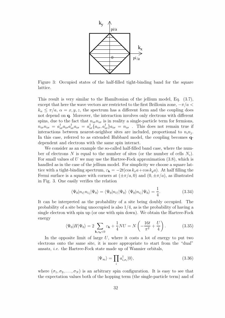
Figure 3: Occupied states of the half-filled tight-binding band for the squarelattice.

This result is very similar to the Hamiltonian of the jellium model, Eq. (3.7),except that here the wave vectors are restricted to the first Brillouin zone, −π/a <kα ≤ π/a, α = x, y, z, the spectrum has a different form and the coupling doesnot depend on q. Moreover, the interaction involves only electrons with differentspins, due to the fact that niσniσ is in reality a single-particle term for fermions,niσniσ = a†iσaiσa

†iσaiσ = a†iσ{aiσ, a

†iσ}aiσ = niσ . This does not remain true if

interactions between nearest-neighbor sites are included, proportional to ninj.In this case, referred to as extended Hubbard model, the coupling becomes q-dependent and electrons with the same spin interact.

We consider as an example the so-called half-filled band case, where the num-ber of electrons N is equal to the number of sites (or the number of cells Nc).For small values of U we may use the Hartree-Fock approximation (3.8), which ishandled as in the case of the jellium model. For simplicity we choose a square lat-tice with a tight-binding spectrum, εk = −2t(cos kxa+cos kya). At half filling theFermi surface is a square with corners at (±π/a, 0) and (0,±π/a), as illustratedin Fig. 3. One easily verifies the relation

〈Ψ0|ni↑ni↓|Ψ0〉 = 〈Ψ0|ni↑|Ψ0〉 〈Ψ0|ni↓|Ψ0〉 =1

4. (3.34)

It can be interpreted as the probability of a site being doubly occupied. Theprobability of a site being unoccupied is also 1/4, as is the probability of having asingle electron with spin up (or one with spin down). We obtain the Hartree-Fockenergy

〈Ψ0|H|Ψ0〉 = 2∑

k,εk<0

εk +1

4NU = N

(

−16t

π2+U

4

)

. (3.35)

In the opposite limit of large U , where it costs a lot of energy to put twoelectrons onto the same site, it is more appropriate to start from the “dual”ansatz, i.e. the Hartree-Fock state made up of Wannier orbitals,

|Ψ∞〉 =∏

i

a†i,σi|0〉, (3.36)

where (σ1, σ2, . . . , σN) is an arbitrary spin configuration. It is easy to see thatthe expectation values both of the hopping term (the single-particle term) and of

32

the two-body interaction vanish, and therefore we get

〈Ψ∞|H|Ψ∞〉 = 0. (3.37)

Comparing the two variational results we conclude that the Bloch point of viewleads to a lower energy for U < Uc := 64t/π2, while for U > Uc the Wannierpicture prevails. One can show that |Ψ0〉 is a metallic state, while |Ψ∞〉 is in-sulating. Therefore our simple variational procedure predicts a metal-insulatortransition as a function of U at a critical value Uc of the order of the bandwidth(8t). This is referred to as the Mott metal-insulator transition. That |Ψ0〉 is ametallic state is clear since this is simply the ground state of a partially filledband of non-interacting electrons. That |Ψ∞〉 is an insulating state appears alsoto be obvious if one imagines to move a particle from its site to a neighboringsite. This leads to double occupancy of the new site and requires an energy U . Itreminds us of conduction in an intrinsic semiconductor, which can only be pro-duced by promoting an electron from the valence to the conduction band, i.e. byproviding the energy difference between the bottom of the conduction band andthe top of the valence band. The main difference is that in the present case theenergy gap U results from the occupation of neighboring sites by other electrons– it is a correlation gap – while a semiconductor has a band gap, generated by theperiodic potential.

Literature

G. D. Mahan, Many-Particle Physics, 2nd edition, Plenum Press, 1990.

H. Bruus and K. Flensberg, Many-Body Quantum Theory in Condensed Matter

Physics, Oxford University Press 2004.

P. Phillips, Advanced Solid State Physics, Westview Press 2003.

33

4 Magnetism

The field of magnetism covers a wide range of important topics, such as the natureof magnetic moments in crystals, Pauli paramagnetism and Landau diamagnetismof conduction electrons, magnetic ordering at low temperatures, the nature ofdomains and domain walls, complex magnetic structures (spin-density waves,spiral phases, ferrimagnetism). Magnetic impurities play an intricate role both inmetals (Kondo effect) and in superconductors (breaking of Cooper pairs). Spinglasses are formed in dilute alloys (such as Cu:Mn) as a result of a competitionbetween disorder and frustration. Subtle phenomena occur in low-dimensionalsystems where strong fluctuations may prevent ordering at finite temperatures.

Magnetic moments are generated both by the orbital motion of charged parti-cles and by the spin (of electrons, protons and neutrons). In solids the electroniccontribution is by far the largest, and in many cases the spin dominates, forinstance in transition metals where the orbital moment of d electrons can bequenched by crystal-field effects. Therefore we will concentrate our attention onthe Heisenberg model, which consists of spins coupled by the exchange interac-tion. It is worth mentioning that the spin, introduced ad hoc in non-relaticisticquantum mechanics to deal both with the anomalous Zeeman effect and withthe Stern-Gerlach experiment, arises naturally in Dirac’s relativistic quantummechanics.

4.1 Exchange

Magnetic order (in insulators) occurs because of the interaction between magneticmoments. The most obvious coupling is purely electromagnetic. A magneticmoment µ1 generates a magnetic field which acts on a second moment µ2 adistance r apart. The result is the dipole-dipole interaction

Hint =µ0

4πr3

(

µ1 · µ2 −r · µ1 r · µ2

r2

)

. (4.1)

This coupling is too weak to explain the ordering in magnetic materials. Never-theless, due to its long-range nature, the dipole-dipole interaction plays an impor-tant role in ferromagnets, where it is responsible for the appearance of magneticdomains.

The origin of magnetic order is exchange, a cooperative effect of Coulombinteraction and Fermi statistics. We consider two electrons for two different situ-ations. In the first case, the two electrons can occupy two different degenerate dorbitals of a single atom, in the second case they can hop between two Wannierstates associated with two neighboring sites of a lattice. We number the twosingle-particle states by the index i = 1, 2 in both cases. We use the parameterU for the on-site Coulomb interaction, as in Eq. (3.27), together with

V = 〈i, j|V2|i, j〉, J = 〈i, j|V2|j, i〉 (4.2)

for i 6= j. We neglect the other terms, therefore the Coulomb interaction of Eq.(3.25) is reduced to

Hint = U(n1↑n1↓ + n2↑n2↓) + V n1n2 − J∑

σ,σ′

a†1σa1σ′a†2σ′a2σ , (4.3)

34

where niσ = a†iσaiσ, ni = ni↑+ni↓. Introducing the (dimensionless) spin operators

Si+ = a†i↑ai↓ ,

Si− = a†i↓ai↑ ,

Siz =1

2(ni↑ − ni↓) , (4.4)

we can rewrite the last term in Eq. (4.3) as −J(12n1n2 + 2S1 · S2). We set the

diagonal contribution of the single-particle term (3.26) equal to zero, by choosingthe zero of energy accordingly, and therefore are left with the Hamiltonian

H = −t∑

σ

(a†1σa2σ+a†2σa1σ)+U(n1↑n1↓+n2↑n2↓)+(V −J2

)n1n2−2J S1·S2 , (4.5)

where t = 0 for the case of two d orbitals on a single atom and t 6= 0 for thetwo-site problem.

To calculate the eigenstates of the Hamiltonian (4.5), we use the fact that Hcommutes with both Sz and S2, where

S = S1 + S2 (4.6)

is the total spin. There are three singlet states (S = 0)

|0, 0〉1 = a†1↑a†1↓|0〉, |0, 0〉2 = a†2↑a

†2↓|0〉, |0, 0〉3 =

1√2(a†1↑a

†2↓ − a†1↓a

†2↑)|0〉, (4.7)

and three triplet states (S = 1)

|1, 1〉 = a†1↑a†2↑|0〉, |1,−1〉 = a†1↓a

†2↓|0〉, |1, 0〉 =

1√2(a†1↑a

†2↓ + a†1↓a

†2↑)|0〉 . (4.8)

The triplet states are eigenstates of the Hamiltonian (4.5),

H|1, m〉 = (V − J)|1, m〉 . (4.9)

In the singlet subspace the Hamiltonian is represented by the 3 × 3 matrix

H →

U 0 −√

2t

0 U −√

2t

−√

2t −√

2t V + 32J

. (4.10)

It is readily diagonalized, giving the three eigenvalues

Es =

{U12

(

U + V + 32J ±

√

(U − V − 32J)2 + 16t2

)

.(4.11)

We consider first the case of two electrons on the same atom (t = 0). Thelargest parameter is usually the term U , in this case the Coulomb energy for twoelectrons with the same wave function. Then the lowest singlet energy, V + 3

2J ,

is higher than the triplet energy, V − J . Thus the direct exchange, the last term

35

in Eq. (4.3), is responsible for Hund’s first rule, according to which the total spinof electrons in a partially filled shell has its maximum possible value.

For the two-site problem we have to take into account the hopping betweensites. The on-site Coulomb term U is again much larger than the other param-eters, including t, at least for typical transition metals. Therefore the lowestsinglet energy is well approximated by

Es,min ≈ V +3

2J − 4t2

U. (4.12)

The eigenstate is essentially |0, 0〉3, with a small admixture of the states |0, 0〉1and |0, 0〉2 (of the order of t/U). Restricting ourselves to this lowest singlet stateand to the three triplet states, we arrive at four states which are to a goodapproximation the eigenstates of the Heisenberg Hamiltonian

H = E0 − Jeff S1 · S2 , (4.13)

where E0 is a constant and

Jeff =5

2J − 4t2

U. (4.14)

Thus the hopping produces a kinetic exchange −4t2/U , which counteracts thedirect exchange 5

2J . In fact, while the direct exchange tends to align the spins

in a triplet state, the kinetic exchange favors a singlet state. In order to get arough idea of the orders of magnitude of the two competing terms, we use theparameters estimated by Hubbard for transition metals: U ≈ 10 eV, J ≈ 0.025eV. With t of the order of 1 eV we find that the kinetic exchange, 4t2/U ≈ 0.4eV, exceeds by far the direct exchange 5

2J . Therefore we expect a strong tendency

towards antiferromagnetic ordering among neighboring transition metal ions.The kinetic exchange can also be obtained from the Hubbard model (where

the direct exchange has been neglected), for U ≫ t and for an average densityof one electron per site. In the limit (t/U) → 0 there are 2N different spinconfigurations (for N electrons on N sites) all of which have energy zero. Forsmall values of (t/U) one uses degenerate perturbation theory to calculate theenergy splitting due to the hopping term. One again arrives at the HeisenbergHamiltonian with exchange constant J = −4t2/U .

4.2 Magnetic order in the Heisenberg model

The Heisenberg Hamiltonian

H = −J∑

〈i,j〉Si · Sj (4.15)

plays an important role for magnetic insulators, both ferromagnetic (J > 0)and antiferromagnetic (J < 0). We have seen above how to arrive at such anexpression with spin 1

2operators. Other values of localized spins occur in many

materials, due to Hund’s first rule. Thus the ion Ni2+ has S = 1, while Cr3+ hasS = 3

2. An important example is the ion Cu2+, which does have a spin 1

2. It occurs

36

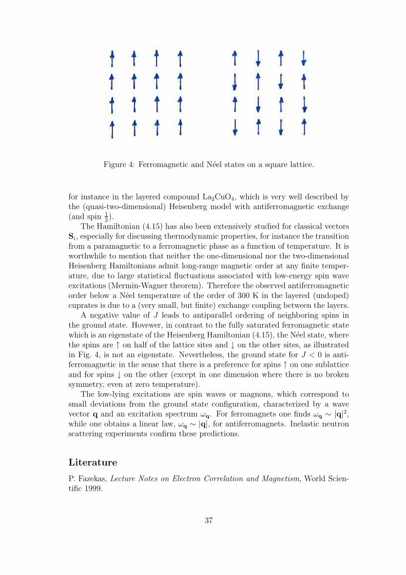
Figure 4: Ferromagnetic and Neel states on a square lattice.

for instance in the layered compound La2CuO4, which is very well described bythe (quasi-two-dimensional) Heisenberg model with antiferromagnetic exchange(and spin 1

2).

The Hamiltonian (4.15) has also been extensively studied for classical vectorsSi, especially for discussing thermodynamic properties, for instance the transitionfrom a paramagnetic to a ferromagnetic phase as a function of temperature. It isworthwhile to mention that neither the one-dimensional nor the two-dimensionalHeisenberg Hamiltonians admit long-range magnetic order at any finite temper-ature, due to large statistical fluctuations associated with low-energy spin waveexcitations (Mermin-Wagner theorem). Therefore the observed antiferromagneticorder below a Neel temperature of the order of 300 K in the layered (undoped)cuprates is due to a (very small, but finite) exchange coupling between the layers.

A negative value of J leads to antiparallel ordering of neighboring spins inthe ground state. Hovewer, in contrast to the fully saturated ferromagnetic statewhich is an eigenstate of the Heisenberg Hamiltonian (4.15), the Neel state, wherethe spins are ↑ on half of the lattice sites and ↓ on the other sites, as illustratedin Fig. 4, is not an eigenstate. Nevertheless, the ground state for J < 0 is anti-ferromagnetic in the sense that there is a preference for spins ↑ on one sublatticeand for spins ↓ on the other (except in one dimension where there is no brokensymmetry, even at zero temperature).

The low-lying excitations are spin waves or magnons, which correspond tosmall deviations from the ground state configuration, characterized by a wavevector q and an excitation spectrum ωq. For ferromagnets one finds ωq ∼ |q|2,while one obtains a linear law, ωq ∼ |q|, for antiferromagnets. Inelastic neutronscattering experiments confirm these predictions.

Literature

P. Fazekas, Lecture Notes on Electron Correlation and Magnetism, World Scien-tific 1999.

37

D.C. Mattis, The Theory of Magnetism I, Springer Series in Solid-State Sciences17, Berlin 1981.

R.M. White, Quantum Theory of Magnetism, McGraw–Hill, New York 1970.

38

5 Electrons and phonons

Until now, whenever we used the word crystal, we assumed the atoms to sit ona perfectly periodic lattice. In reality, atoms oscillate around their equilibriumpositions, even at zero temperature. The quantum of vibration is a phonon.Phonons contribute to the specific heat of crystals, to the thermal expansionand to the melting of a crystal (through anharmonicities), and they give riseto the electrical resistance via the electron-phonon interaction. Last but notleast, the exchange of phonons between two electrons may provide an effectiveattraction and lead to superconductivity. In this short chapter, we limit ourselvesto three topics, the phonons in a harmonic crystal, the origin of the electron-phonon interaction and the effective electron-electron attraction resulting fromphonon exchange.

5.1 The harmonic crystal

The theory of lattice dynamics is based on the assumption that the atomic dis-placements are small. In the harmonic approximation, the expansion of the po-tential energy in powers of the displacements is carried out up to the secondorder. For simplicity, we consider the case of one atom per unit cell. The atomicpositions are given by R + u(R), where the vectors R span a three-dimensionalBravais lattice and the vectors u(R) are the atomic displacements away fromequilibrium. Every atom has three degrees of freedom described by the threecomponents of the displacement vector uα(R), α = x, y, z . In the harmonic ap-proximation the Hamiltonian is given by

H =1

2M

∑

R,α

p2α(R) +

1

2

∑

R,R′

α,β

Dα,β(R −R′)uα(R)uβ(R′) , (5.1)

where pα(R) are the components of the atomic momentum at R andD(R− R′) isthe dynamical matrix, the second derivative of the potential energy with respectto the atomic displacements at R and R′ . There is no linear term since weassume to start from equilibrium, where there is no force acting on the atoms.The transformation

u(R) =1√NM

∑

k,λ

qk,λ ek,λ eik·R ,

p(R) =

√

M

N

∑

k,λ

pk,λ ek,λ eik·R , (5.2)

where N is the number of unit cells, ekλ (λ = 1, 2, 3) are the three orthonor-mal eigenvectors of the Fourier transform D(k) of the dynamical matrix witheigenvalues Mω2

k,λ, leads to

H =1

2

∑

k,λ

(pk,λp−k,λ + ω2

k,λ qk,λq−k,λ

). (5.3)

39

To quantize the theory, we replace the canonical variables u(R) and p(R) byoperators satisfying the commutation relations

[uα(R), uβ(R′)] = [pα(R), pβ(R

′)] = 0,

[uα(R), pβ(R′)] = i~ δR,R′ δα,β . (5.4)

This leads to

[qk,λ, qk′,λ′] = [pk,λ, pk′,λ′] = 0,

[qk,λ, pk′,λ′] = i~ δλ,λ′ δk,−k′ . (5.5)

Finally, introducing phonon creation and annihilation operators b†k,λ and bk,λ ,respectively,

qk,λ =

√

~

2ωk,λ

(

bk,λ + b†−k,λ

)

pk,λ = −i√

~ωk,λ

2

(

bk,λ − b†−k,λ

)

, (5.6)

with commutation relations

[bk,λ, bk′,λ′ ] =[

b†k,λ, b†k′,λ′

]

= 0 ,[

bk,λ, b†k′,λ′

]

= δk′,kδλ,λ′ , (5.7)

we obtain the familiar Hamiltonian of a collection of independent bosons

H =∑

k,λ

~ωk,λ

(

b†k,λbk,λ +1

2

)

. (5.8)

The dynamical matrix has both inversion symmetry,

Dαβ(R −R′) = Dαβ(R′ − R) (5.9)

and continuous translational symmetry,∑

R

Dαβ(R) = 0 . (5.10)

Its Fourier transform D(k) can therefore be rewritten as

D(k) =1

2

∑

R

(e−ik·R + eik·R − 2

)D(R) = −2

∑

R

sin2 k ·R2

D(R) . (5.11)

It follows that D(k) ∼ k2 for k → 0 (provided that D(R) decreases sufficientlyfast for R → ∞). Therefore the eigenvalues of D(k) have dispersion relations

ω2k,λ ∼ c2λk

2 for k → 0, λ = 1, 2, 3 , (5.12)

corresponding to acoustic phonons, two “transverse” modes and one “longitudi-nal” mode, with sound velocities cλ .

40

5.2 Electron-phonon interaction

To describe the coupling between an electron and the acoustic phonons, we usea simple “rigid ion” model. Each ion represents for the electron a potential Va,which depends on the distance between the position r of the electron and theionic position R + u(R). Assuming these contributions to add up, we obtain thepotential V (r) acting on the electron

V (r) =∑

R

Va(r − R − u(R)) ≈∑

R

Va(r −R)−∑

R

∇Va(r −R) ·u(R) . (5.13)

The first term of the Taylor expansion is a periodic potential leading to Blocheigenstates for the electron, the second term represents the electron-phonon in-teraction

Vep(r) := −∑

R

∇Va(r − R) · u(R) . (5.14)

In order to treat a many-electron system (the partially filled conduction band of ametal), we write Vep(r) in second-quantized representation, using the Bloch statesas single-particle basis. For simplicity, we restrict ourselves to a single band with(Bloch) wave function

ψk(r) = eik·ruk(r) , (5.15)

where k is a vector of the first Brillouin zone and uk(r) = uk(r + R). Using theFourier transform,

Va(r) =1

V

∑

q

Va(q) eiq·r (5.16)

together with Eqs. (5.2) and (5.6), we get

〈k|Vep|k′〉 = − 1V

∑

q,q′,λ Va(q)√

~

2NMωq′λiq · eq′λ

∑

R e−i(q−q′)·R(bq′λ + b†−q′λ)

∫

Vd3r e−i(k−k′−q)·r u∗k(r) uk′(r) . (5.17)

We use the relation ∑

R

e−i(q−q′)·R = N∆(q − q′) , (5.18)

where

∆(q) =

{1, if q is a reciprocal lattice vector0, otherwise.

(5.19)

Similarly, the matrix elements∫

Vd3r e−i(k−k′−q)·r u∗k(r) uk′(r) are only non-zero

if k − k′ − q is a reciprocal lattice vector. We neglect Umklapp processes whichinvolve finite reciprocal lattice vectors. Moreover, the acoustic modes consist(approximately) of one longitudinal and two transverse modes, among whichonly the longitudinal mode contributes, with q · eq = |q|, ωq = sq. With thesesimplifications we obtain (k′ = k − q)

〈k|Vep|k − q〉 = gk,q(bq + b†−q) , (5.20)

where the electron-phonon coupling constant is

gk,q = − i

VVa(q)

√

~Nq

2Ms

∫

V

d3r u∗k(r) uk−q(r) . (5.21)

41

Figure 5: Electron-phonon scattering process.

The second-quantized representation of the electron-phonon interaction is thengiven by

Hep =∑

k,q,σ

gk,q(bq + b†−q)a†kσak−qσ , (5.22)

where a†kσ and akσ are, respectively, creation and annihilation operators of elec-trons with wavevector k and spin σ. Hep corresponds to the scattering processdepicted in Fig. 5.

5.3 Phonon-induced attraction

The fundamental interactions in metals are the Coulomb interaction betweenelectrons and the electron-phonon interaction. A thorough treatment of bothinteractions would require advanced techniques, such as the Green function for-malism. These techniques are able to show that the Coulomb interaction, whichdecays very slowly in an insulator, not only is screened in a metal and thusbecomes short ranged, but it even may be “overscreened” due to the electron-phonon interaction and change sign. Here we use a plausibility argument for theorigin of an effective attraction, as proposed by H. Frohlich several years beforethe BCS theory. We consider the Hamiltonian of (conduction) electrons coupledto (longitudinal acoustic) phonons,

H =∑

kσ

εka†kσakσ +

∑

q

~ωqb†qbq +

∑

k,q,σ

gk,q(bq + b†−q)a†kσak−qσ . (5.23)

We use stationary state perturbation theory in powers of the electron-phononcoupling, starting from the bare ground state,

|Ψ0〉 =∏

k,σεk<εF

a†kσ|0〉e ⊗ |0〉p , (5.24)

where the electronic levels are filled up to the Fermi level and there is no phonon.The first order contribution to the energy vanishes. The second order contribution

42

can be written as

∆E = 2∑

k,k′

(1 − fk)fk′

|gk,k−k′|2εk′ − εk − ~ωk−k′

, (5.25)

where fk is the Fermi-Dirac function at zero temperature,

fk =

{1, εk < εF

0, εk > εF .(5.26)

The symmetry |gk,k−k′|2 = |gk′,k′−k|2 allows us to rewrite Eq. (5.25) as

∆E = 2∑

k

fk∑

k′

|gk,k−k′|2εk − εk′ − ~ωk′−k

+ 2∑

k,k′

fkfk′

|gk,k−k′|2~ωk−k′

(~ωk−k′)2 − (εk − εk′)2. (5.27)

This expression can be interpreted as arising from a purely electronic Hamiltonian

H =∑

kσ

(εk + ∆εk)a†kσakσ +

1

2V

∑

k,k′,qσ,σ′

∆v(k,k′,q) a†kσa†k′σ′ak′+qσ′ak−qσ , (5.28)

where the single particle spectrum has been renormalized, εk → εk + ∆εk with

∆εk =∑

k′

|gk,k−k′|2εk − εk′ − ~ωk′−k

, (5.29)

and an effective electron-electron interaction has been induced by phonon ex-change, with coupling

∆v(k,k′,q) = 2V|gk,q|2~ωq

(εk − εk′)2 − (~ωq)2. (5.30)

In fact, first order perturbation theory with respect to ∆ε and ∆v gives

∆E = 2∑

k

fk∆εk

+1

V

∑

k,k′

fkfk′ [2∆v(k,k′, 0) − ∆v(k,k′,k − k′)] . (5.31)

The Hartree term with momentum transfer zero vanishes since g(k,q = 0) = 0.Therefore we recover indeed Eq. (5.27). The crucial point is that the effectivecoupling function (5.30) is attractive for |εk − εk′| < ~ωk−k′. A more elaboratetreatment using the technique of Green functions confirms that close to the Fermisurface the electron-phonon interaction leads to an effective attraction.

43

6 Superconductivity: BCS theory

The aim of this chapter is to present the BCS theory, the probably most successfulmicroscopic description of a collective quantum phenomenon. Another importanttheory, the Ginzburg-Landau theory, does not depend on microscopic detailsbut rather establishes a general phenomenological framework for the transitionfrom the normal to the superconducting phase. We will limit ourselves to themicroscopic BCS theory.

6.1 Cooper pairs

From now on it will be assumed that the electron-phonon interaction (or possiblyalso the exchange of another type of boson, for instance a magnon) can producean effective attraction beween electrons. If the attractive interaction is strongenough, two electrons may form a bound state or composite boson. In such acase it is tempting to develop a model for superconductivity in terms of a Bose-Einstein condensation of electron pairs. However, for ordinary superconductorsthe attraction is not strong enough to produce a two-electron bound state (exceptin one and two dimensions). The reason is that in three dimensions the single-particle density of states

N(ε) =1

V

∑

k

δ(ε− εk) (6.1)

tends to zero for ε → 0 (in the case of a parabolic spectrum). Cooper realizedthat the situation is different if we add two electrons to the filled Fermi sea (andnot to the vacuum).

For simplicity, we limit ourselves on that part of the Hamiltonian which isrelevant for both the Cooper problem and the BCS theory, the so-called reducedHamiltonian

Hred =∑

k,σ

εka+kσakσ +

1

V

∑

k,k′

v(k,k′) a+k↑a

+−k↓a−k′↓ak′↑ . (6.2)

For the Cooper problem we assume v(k,k′) to be attractive in a finite strip abovethe Fermi energy,

v(k,k′) =

{−g , εF < εk, εk′ < εF + ~ωD ,0 , otherwise,

(6.3)

where the Debye frequency ωD is the characteristic scale of acoustic phonons. Anadded pair with total momentum zero and Sz = 0 is described by the state

|Ψ〉 =∑

k

ϕ(k)a+k↑a

+−k↓|F〉 . (6.4)

We look for an eigenstate of energy E. Applying the reduced Hamiltonian on thepair state we get

Hred|Ψ〉 =∑

k

ϕ(k)(E0 +2εk)a+k↑a

+−k↓|F〉+

1

V

∑

k,k′

ϕ(k)v(k′,k)a+k′↑a

+−k′↓|F〉 , (6.5)

44

where E0 is the energy of the filled Fermi sea. Multiplying from the left by〈F|a−k′↓ak′↑, we obtain the eigenvalue equation

ϕ(k′)(E0 + 2εk′ − E) +1

V

∑

k

ϕ(k)v(k′,k) = 0. (6.6)

Using Eq. (6.3) and summing over k′ we arrive at the relation

1 =g

V

∑

k′

′ 1

E0 + 2εk′ −E, (6.7)

where the sum is restricted to the energy strip defined above. In the absence ofinteractions the lowest possible energy for a filled Fermi sea plus two additionalelectrons is E = E0 +2εF . Therefore the quantity εb := E−E0 − 2εF defines thebinding energy due to the attractive coupling. With the density of states (6.1)Eq. (6.7) can be rewritten as

1 = g

∫ εF +~ωD

εF

N(ε)

2(ε− εF ) − εb

≈ gN(εF )

∫ εF +~ωD

εF

1

2(ε− εF ) − εb

, (6.8)

where we have assumed that N(ε) does not change appreciably on the scale~ωD ≪ εF . The integration is elementary and we obtain the interesting relationfor the binding energy

εb ≈ 2~ωDe− 2

gN(εF ) . (6.9)

This is a non-analytic function, which cannot be obtained by a finite-order per-turbation expansion.

6.2 BCS ground state

For a very low density of electrons and strong attraction we expect the systemto consist of bound (bosonic) pairs, which may undergo a Bose-Einstein conden-sation at low temperatures. Eq. (6.4) is then a good starting point and we canconsider the operator

b+q=0 :=∑

k

ϕ(k)a+k↑a

+−k↓ (6.10)

approximately as a bosonic creation operator with momentum zero. Neglectingthe residual interaction between the pairs we can write down the ground state ofN2

pairs as a Bose condensate

|BEC〉 =1

√

(N/2)!

(b+q=0

)N2 |0〉 . (6.11)

In the weak coupling limit (high density and weak attraction) the BCS state,which describes the instability of the Fermi surface with respect to a coherentpairing, is more appropriate. It is defined as

|BCS〉 =∏

k

(

uk + vka†k↑a

†−k↓

)

|0〉 , (6.12)

45

where the coefficients uk, vk are variational parameters. The BCS state is nor-malized if

u2k + v2

k = 1. (6.13)

In this state the number of particles is not fixed, but this is not a problem inthe thermodynamic limit (as in statistical mechanics, where the grand canonicalensemble produces the same thermodynamics as the canonical ensemble). Wecan obtain the projection of the BCS state onto the subspace with a fixed (even)number N of electrons as follows. We observe that (a†k↑a

†−k↓)

n vanishes for n ≥ 2.Therefore we can write

uk + vka†k↑a

†−k↓ = uk

(

1 +vkuk

a+k↑a

+−k↓

)

= uk exp

(vkuk

a+k↑a

+−k↓

)

. (6.14)

The BCS state then reads

|BCS〉 = const exp

(∑

k

vkuk

a+k↑a

+−k↓

)

|0〉 . (6.15)

Its projection onto the subspace with N electrons,

|BCS〉N = const’

(∑

k

vkuk

a+k↑a

+−k↓

)N2

|0〉 , (6.16)

is equal to Eq. (6.11) except that the wave function ϕ(k) has been replaced byvkuk

. The calculations are much simpler for the full BCS state (6.12) than for theprojected state.

We have to minimize the expectation value of the reduced Hamiltonian (6.2),〈BCS|Hred|BCS〉, for a given average number of electrons

N = 〈BCS|N |BCS〉, where N =∑

k,σ

a+kσakσ . (6.17)

This is carried out by introducing the chemical potential µ as a Lagrange multi-plier. Thus we have to minimize first the expression

W := 〈BCS|Hred − µN |BCS〉 (6.18)

and at the end fix µ by solving Eq. (6.17).We use a similar model for the attraction as in the Cooper problem and restrict

the coupling to a strip of width 2~ωD around the chemical potential µ (which isapproximately equal to the Fermi energy εF in the weak-coupling limit).

v(k,k′) =

{−g, µ− ~ωD < εk, εk′ < µ+ ~ωD ,0, otherwise.

(6.19)

The single-particle states outside this strip are not affected and we have

uk =

{0, εk < µ− ~ωD ,1, εk > µ+ ~ωD .

vk =

{1, εk < µ− ~ωD ,0, εk > µ+ ~ωD .

(6.20)

46

With the parametrization

uk = cosϑk , vk = sinϑk (6.21)

the relation (6.13) is automatically satisfied.It is straightforward to calculate the expectation value (6.18). One finds

W = 2∑

k

ξkv2k −

g

V

∑

k,k′

ukvkuk′vk′

=∑

k

ξk(1 − cos 2ϑk) − g

4V

(∑

k

sin 2ϑk

)2

, (6.22)

where ξk := εk − µ. (The diagonal term of the interaction energy, k = k′ , is notcorrect, but this error is negligible in the thermodynamic limit.) The signs haveto be chosen such as to render this expression as small as possible. The sign ofsin 2ϑk is arbitrary (we choose sin 2ϑk > 0), but not that of cos 2ϑk which has tofulfill

sign(cos 2ϑk) = sign(ξk) (6.23)

because W is required to be a minimum. Moreover, the equation ∂W/∂ϑk = 0leads to

ξk tan 2ϑk =g

2V

∑

k′

sin 2ϑk′ , (6.24)

where both k and k′ are in the region of k-space defined above. Introducing the(positive) gap parameter

∆k := ξk tan 2ϑk , (6.25)

we can write Eq. (6.24) as

∆k =g

2V

∑

k′

∆k′

Ek′

, (6.26)

where

Ek :=√

ξ2k + ∆2

k . (6.27)

With

∆k =

{∆0 , |ξk| < ~ωD ,0 , otherwise ,

(6.28)

and the replacement

1

V

∑

k

f(ξk′) → N(εF )

∫~ωD

−~ωD

dξ f(ξ) (6.29)

the gap equation (6.26) becomes

1 =g

2N(εF )

∫~ωD

−~ωD

dξ1

√

ξ2 + ∆20

. (6.30)

This equation is readily solved, we get

∆0 = ~ωD1

sinh 1gN(εF )

≈ 2~ωDe− 1

N(εF )g , (6.31)

47

where the approximate expression is valid in the weak-coupling limit, gN(εF ) ≪1. This result resembles the binding energy of a Cooper pair, Eq. (6.9), it is againa non-analytic function of the coupling strength.

In the strong-coupling limit one can show that the gap equation (6.26) isnothing but the eigenvalue equation (6.6) “in disguise” (A. J. Leggett, Proc.16th Karpacz Winter School, Lecture Notes in Physics 115, Springer 1980, p.13). The BCS state describes in fact a smooth crossover from a coherent many-electron bound state (with “pair size” larger than the interpair distance and achemical potential µ ≈ εF ) for weak coupling to a Bose condensate of bound pairs(with µ < 0) for strong coupling.

The physical meaning of Ek can be understood by calculating the energyrequired for adding an electron with momentum ~k to the system. This quasi-

particle energy is just equal to Ek (see J. R. Schrieffer, Theory of Superconduc-

tivity, Section 2.5).

6.3 Thermodynamics

It is straightforward to generalize the BCS theory to finite temperatures T , usinga self-consistent field method. Here we simply quote the main results and usethem to calculate the specific heat.

For T > 0 the gap parameter becomes temperature dependent. Eq. (6.26) isreplaced by (β = 1

kBT)

∆k =g

2V

∑

k′

∆k′

Ek′

tanhβEk′

2, (6.32)

which goes over into Eq. (6.26) for T → 0. Proceeding as above we obtain thefinite temperature gap equation

1 =g

2N(εF )

∫~ωD

−~ωD

dξ1

√

ξ2 + ∆2tanh

(β

2

√

ξ2 + ∆2

)

. (6.33)

The r.h.s. is a decreasing function of both T and ∆. It follows that the solutionof Eq. (6.33), ∆(T ), decreases with increasing temperature until it vanishes ata critical temperature Tc. For weak coupling (kBTc ≪ ~ωD) the function ∆(T ),depicted in Fig. 6, is universal. For T = 0 the solution of the gap equation isgiven by Eq. (6.31). For T = Tc partial integration gives

1 = gN(εF )

∫ βc~ωD

0

dy1

ytanh

y

2

= gN(εF )

[

log(βc~ωD) tanhβc~ωD

2− 1

2

∫ βc~ωD

0

dy log y sech2 y

2

]

.

In the last term we can replace βc~ωD by ∞ (in the weak coupling limit) and use

−1

2

∫ ∞

0

dy log y sech2y

2= log

(2γ

π

)

,

48

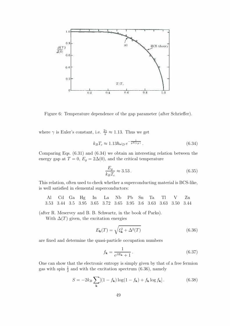
Figure 6: Temperature dependence of the gap parameter (after Schrieffer).

where γ is Euler’s constant, i.e. 2γπ≈ 1.13. Thus we get

kBTc ≈ 1.13~ωD e− 1

gN(εF ) . (6.34)

Comparing Eqs. (6.31) and (6.34) we obtain an interesting relation between theenergy gap at T = 0, Eg = 2∆(0), and the critical temperature

Eg

kBTc

≈ 3.53 . (6.35)

This relation, often used to check whether a superconducting material is BCS-like,is well satisfied in elemental superconductors:

Al Cd Ga Hg In La Nb Pb Sn Ta Tl V Zn3.53 3.44 3.5 3.95 3.65 3.72 3.65 3.95 3.6 3.63 3.63 3.50 3.44

(after R. Meservey and B. B. Schwartz, in the book of Parks).With ∆(T ) given, the excitation energies

Ek(T ) =√

ξ2k + ∆2(T ) (6.36)

are fixed and determine the quasi-particle occupation numbers

fk =1

eβEk + 1. (6.37)

One can show that the electronic entropy is simply given by that of a free fermiongas with spin 1

2and with the excitation spectrum (6.36), namely

S = −2kB

∑

k

[(1 − fk) log(1 − fk) + fk log fk] . (6.38)

49

The presence of the gap implies that in the superconducting phase the entropy islower than it would be for ∆ = 0 (see Fig. 7). The superconducting phase has ahigher degree of order than the normal phase. The specific heat per unit volumeis given by

CV

V=

T

V

∂S

∂T=

2

V

∑

k

Ek

∂fk∂Ek

(∆

Ek

d∆

dT− Ek

T

)

≈ 2N(εF )

∫ ∞

−∞dξ

(1

2

d∆2

dT− E2

T

)∂f

∂E, (6.39)

where E =√

ξ2 + ∆2. Close to Tc, where

∆(T )

∆(0)∼ 1.74

(Tc − T

Tc

) 12

, (6.40)

the derivative d∆2

dTis finite when approaching Tc from below and it vanishes for

T > Tc, where the specific heat is given by the usual expression

C(n)V

V= γT =

2π2

3N(εF )k2

BT .

It follows that there is a step at Tc

C(s)V − C

(n)V

C(n)V

≈ 1.43 , (6.41)

in quite good agreement with experiments on elemental superconductors:

Al Cd Ga Hg In La Nb Pb Sn Ta Tl V Zn1.4 1.4 1.4 2.37 1.73 1.5 1.9 2.71 1.60 1.59 1.50 1.49 1.3

(after R. Meservey and B. B. Schwartz, in the book of Parks). The BCS predictionfor the specific heat is illustrated in Fig. 7.

We did not discuss the most striking phenomena of superconductivity, suchas persistent currents, Meissner effect, flux quantization or Josephson tunneling.This would require to extend BCS theory by adding the coupling to an electro-magnetic field. We do not present this extension here, but simply mention thatthis coupling can be readily obtained in BCS theory in terms of the standardreplacement (see, for instance, Chapter 8 of Schrieffer’s book)

p → p + eA, i~∂

∂t→ i~

∂

∂t− eΦ. (6.42)

50

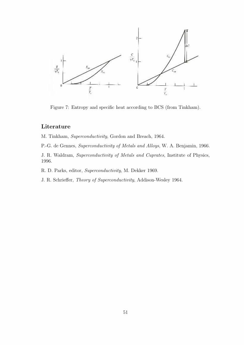
Figure 7: Entropy and specific heat according to BCS (from Tinkham).

Literature

M. Tinkham, Superconductivity, Gordon and Breach, 1964.

P.-G. de Gennes, Superconductivity of Metals and Alloys, W. A. Benjamin, 1966.

J. R. Waldram, Superconductivity of Metals and Cuprates, Institute of Physics,1996.

R. D. Parks, editor, Superconductivity, M. Dekker 1969.

J. R. Schrieffer, Theory of Superconductivity, Addison-Wesley 1964.

51