Progress of Theoretical Physics, Supplement 150 (2003) 64-80

Nonlinear Dynamics and Chaos in Many-Particle Hamiltonian Systems

Pierre GaspardCenter for Nonlinear Phenomena and Complex Systems

Universite Libre de Bruxelles, Code Postal 231, Campus Plaine, B-1050 Brussels, Belgium

We report the results of studies of nonlinear dynamics and dynamical chaos in Hamiltoniansystems composed of many interacting particles. The importance of the Lyapunov exponents andthe Kolmogorov-Sinai entropy is discussed in the context of ergodic theory and nonequilibriumstatistical mechanics. Two types of systems are studied: hard-ball models for the motion of a traceror Brownian particle interacting with the particles of a surrounding fluid and microplasmas whichare composed of positively charged ions confined in a Penning electromagnetic trap. Lyapunovexponents are studied for both classes of systems. In microplasmas, transitions between differentregimes of nonlinear behavior and chaos are reported.

I. INTRODUCTION

The motion of atoms, molecules or ions in gases, liquids, solids, or plasmas is known to be Hamiltonian. ThisHamiltonian character finds its origin in the unitarity of the underlying quantum dynamics. In the classical limitwhere the de Broglie wavelength is much smaller than distances between the particles, Hamiltonian classical mechanicsemerges from the underlying quantum dynamics. Typically, Hamilton’s equations are nonlinear so that the classicaldynamics presents a rich variety of nonlinear behavior, such as bifurcations between different regimes as well asdynamical chaos. Today, it is possible to provide a quantitative characterization of the sensitivity to initial conditionsas well as of the dynamical randomness, which are two fundamendal properties of chaotic systems. The sensitivity toinitial conditions is characterized by the Lyapunov exponents which are the rates of exponential separation betweentwo nearby trajectories, and the dynamical randomness by the so-called Kolmogorov-Sinai (KS) entropy per unit time[1].

Recently, much work has been devoted to many-particle systems and to their chaotic dynamics in the context ofnonequilibrium statistical mechanics [2–12]. In this field, the assumption of dynamical chaos has the advantage tobe compatible both with the determinism of the microscopic dynamics and with the known existence of dynamicalrandomness in the systems of statistical mechanics. In microscopic systems of particles, the time scale of dynamicalchaos is of the order of the short intercollisional time. On the other hand, the transport properties are the featureof the long hydrodynamic time scale. Relationships between between chaos and transport have been established inHamiltonian systems thanks to the escape-rate theory [2, 13–15] and the hydrodynamic-mode theory [16–18]. Inboth theories, the transport coefficients are related to differences between characteristic quantities of chaos such asthe Lyapunov exponents or the KS entropy, bridging in this way the gap of time scales. Furthermore, methodsof statistical mechanics have been developed in order to calculate the Lyapunov exponents and the KS entropy ofmany-particle systems such as dilute gases of identical particles [19–23]. The new methods and results are particularlysuitable to understand the behavior of mesoscopic systems and the way the macroscopic properties themselves emergein the thermodynamic limit. The nanoscopic or mesoscopic systems contains several dozens, hundreds, or thousandsof particles, which form finite dynamical systems. Their dynamical and kinetic properties is beginning to be explored.

The purpose of the present paper is to contribute to the study of nonlinear dynamics and dynamical chaos in many-particle Hamiltonian systems. Results are presented for two types of systems, which are of experimental relevance.

The first type of systems are models of Brownian motion. The particles are hard balls, i.e., hard disks in twodimensions or hard spheres in three dimensions. The system is composed of a hard ball representing a tracer orBrownian particle, together with many other hard balls for the surrounding fluid. The interaction between theparticles has a short range and the time evolution of this system can be efficiently simulated by an event-drivenalgorithm. This method allows us to obtain the spectrum of Lyapunov exponents. An interesting question whichhas recently been investigated is to know the conditions under which the tracer or Brownian particle dominates theLyapunov spectrum [24].

The second type of systems are microplasmas, which are composed of positively charged ions confined in some Paulor Penning electromagnetic traps [25–29]. These systems are among the first where individual microscopic particleshave been observed. Recent work has shown that even their trajectories can be observed. It is therefore possible forthese systems to detect the nature of the microscopic dynamics. In the present paper, we show theoretically thatthe motion has regular features at low kinetic energy and that chaotic motion becomes dominant at higher energy to

2

decrease at still higher energy because of the trapping potential.The paper is organized as follows. Generalities about Hamiltonian mechanics and the linear stability of its tra-

jectories are summarized in Sec. II. In Sec. III, we explain the place of dynamical chaos in ergodic theory andnonequilibrium statistical mechanics. Results on the models of tracer and Brownian motions are given in Sec. IV.The nonlinear dynamics and chaotic behavior of microplasmas are described in Sec. V. Conclusions and perspectivesare discussed in Sec. VI.

II. HAMILTONIAN MECHANICS AND SENSITIVITY TO INITIAL CONDITIONS

A Hamiltonian classical system of N particles is defined in the phase space M of the positions and momenta of theparticles: Γ = (r1,p1, ..., rN ,pN ). The equations of motion are given in terms of the Hamiltonian function H(Γ ) as

dΓdt

= −J · grad H , (1)

where J is the 2f × 2f fundamental symplectic matrix

J =(

0 −I+I 0

). (2)

According to Cauchy’s theorem, trajectories from given initial conditions Γ0 are unique so that Hamilton’s equationsdefine a flow in the phase space. This flow is a one-parameter Lie group,

Γt = Φt(Γ0) , (3)

the parameter being the time t.The Jacobian matrix of the flow

St =∂Φt

∂Γ, (4)

is a symplectic matrix satisfying

STt · J · St = St · J · ST

t = J . (5)

A consequence of the symplectic character is that the determinant of the Jacobian matrix is always equal to unity:

|detSt| = 1 , (6)

which implies Liouville’s theorem according to which phase-space volumes are preserved during a Hamiltonian timeevolution. The Jacobian matrix rules the time evolution of infinitesimal perturbations δΓt on the trajectories

δΓt = St(Γ0) · δΓ0 . (7)

The linear stability of the trajectories can be characterized in terms of the Lyapunov exponents which are thegrowth rates of the infinitesimal perturbations

λ(Γ0, δΓ0) = limt→∞

1t

ln‖δΓt‖‖δΓ0‖

, (8)

with ‖δΓ‖ = (δΓT · δΓ )1/2. A Lyapunov exponent is associated with each trajectory Γ0 and each initial perturbationδΓ0. Since the Jacobian matrix of Hamiltonian system is symplectic, the Lyapunov exponents obey a pairing rule,which says that, if λ is a Lyapunov exponent, then −λ is also a Lyapunov exponent.

Systems with positive Lyapunov exponent are dynamically unstable, i.e., their trajectories are sensitive to the initialconditions. Predictions on the time evolution of such systems are thus limited by the accuracy on the knowledge ofthe initial conditions. Prediction on a trajectory remains realistic as long as the time is smaller than the Lyapunovtime which depends on the initial ‖δΓ0‖ and final ‖δΓt‖ accuracies:

t < tLyapunov =1λ1

ln‖δΓt‖‖δΓ0‖

, (9)

λ1 being the maximum Lyapunov exponent. Hence, the Lyapunov time constitutes a horizon for the prediction onthe future time evolution. Beyond the Lyapunov time, prediction is no longer possible and a statistical description isrequired.

3

III. INVARIANT PROBABILITY, ERGODICITY, MIXING, AND CHAOS

In a statistical description, the average of an observable A is given in terms of a probability density ρ as

〈A〉 =∫

A(Γ ) ρ(Γ ) dΓ , (10)

where dΓ denotes the invariant Liouvillian Lebesgue measure in phase space. The time evolution of the probabilitydensity obeys the Liouville equation

∂t ρ = −div(Γρ

)= H, ρ ≡ Lρ , (11)

where ·, · denotes the Poisson bracket.Systems of particles such as gases, liquids, solids, or plasmas are the stage of several types of processes, from the

transport processes on the long hydrodynamic time scale down to kinetic processes on the short intercollisional timescale. These time-dependent processes have in common that they are described in terms of time auto- or cross-correlation functions, measuring the statistical correlations between events which are separated in time. In particular,the transport coefficients are given by the Green-Kubo formulas as the time integrals of the two-time correlationfunctions of associated microscopic currents [30, 31]. Similarly, light or neutron scattering signals are also describedin terms of two-time correlation functions [32]. On the other hand, the nonlinear optical properties or NMR multipulsesignals depend on multiple-time correlation functions [33].

In many-particle systems, these time correlation functions usually decay to their asymptotic values when the eventsare arbitrarily separated in time. This fundamental property is called mixing or multiple mixing. The mixingproperty has been introduced by Gibbs and ergodic theory has shown that mixing (and already weak mixing) impliesergodicity, i.e., the equality of time and phase-space averages with respect to an invariant probability measure µ [34].This probability measure describes the statistical properties of the system. The invariance of the probability measureis established with respect to the equations of motion ruling the time evolution of the system. An invariant measurehas a density satisfying Lρ = 0.

The system can be either in thermodynamic equilibrium if its pressure, temperature, and chemical potentials areuniform, or out of equilibrium if nonequilibrium constraints are imposed at the boundaries allowing fluxes of energy ormatter to circulate across the system. Different invariant measures correspond to these different physical situations.Well-known equilibrium invariant measures are the microcanonical measure for an isolated system at given energy andthe canonical measure for a closed system at given temperature. Recent work has been devoted to the determinationof nonequilibrium invariant measures [8, 35].

A remarkable result is that a deterministic system together with one of its invariant probability measures definesa random processes. As a consequence, a deterministic system can generate dynamical randomness, which is char-acterized by an entropy per unit time, a quantity measuring the disorder of the trajectories along the time axis.The concept of entropy per unit time has been introduced by Shannon in his mathematical theory of communication[36], by analogy with the standard Boltzmann entropy measuring a spatial disorder in a thermodynamic system.Kolmogorov and Sinai thereafter established a rigorous definition of entropy per unit time for dynamical systems andother random processes [34]. A concept of space-time entropy or entropy per unit time and unit volume was laterintroduced by Sinai and Chernov [37].

The KS entropy is based on the idea that the dynamics Φt is observed by making a partition P of its phase spaceinto cells of labels ω [1, 34]. If the system is observed with a sampling time ∆t we can determine the probabilitiesµ(ω0ω1ω2...ωn−1) that its trajectories will successively visit the cells ω0ω1ω2...ωn−1. The entropy per unit time of thesystem with respect to the chosen partition is then defined as

h(Φ∆t,P) = limn→∞

− 1n∆t

∑ω0ω1ω2...ωn−1

µ(ω0ω1ω2...ωn−1) lnµ(ω0ω1ω2...ωn−1) . (12)

For differentiable dynamical systems, this entropy per unit time does not depend on the sampling time ∆t. Never-theless, this entropy still depends on the partition P. In order to get rid of this arbitrariness which is due to thespecifications of the measuring device, Kolmogorov and Sinai have considered the supremum of the entropy withrespect to all the possible partitions

hKS = SupPh(Φ∆t,P) , (13)

which is a number characterizing an intrinsic property of the dynamics Φt with respect to the invariant probabilitymeasure µ. In fact, the KS entropy per unit time characterizes the dynamical randomness which is generated by the

4

dynamics during the time evolution. A dynamical system with a positive KS entropy thus behaves as a pseudo-randomgenerator which would be repetitively called during time evolution at a frequency given by the ratio of the system KSentropy over the entropy of the random variable of the pseudo-random generator.

The KS entropy is a powerful concept because this simple quantity controls the top of the hierarchy of ergodicproperties [34]:

K property ⇒ multiple mixing ⇒ mixing ⇒ weak mixing ⇒ ergodicity . (14)

The Kolmogorov or K property holds if there exists a subalgebra of measurable sets in phase space which generatesthe whole algebra by application of the flow [34]. The K property is equivalent to saying that the unitary operatorU tf(Γ ) = f(ΦtΓ ) = e−Ltf(Γ ) has a Lebesgue continuous spectrum of countable multiplicity. The remarkable resultis that the K property at the top of the ergodic hierarchy can be expressed in terms of the entropy per unit timeaccording to the following theorem [34]:

A system Φt has the Kolmogorov property if h(Φ1,P) > 0 for any finite partition P 6= ∅,M.The fact that a system has a positive KS entropy does not imply that the entropy h(Φ1,P) will be positive for everynontrivial partition. Nevertheless, a chaotic system will have strong mixing properties, at least, on parts of its phasespace. In this sense, a positive KS entropy can justify the existence of a strong mechanism of relaxation in some partsof the phase space of the system.

The dynamical randomness of a deterministic system finds its origin in the dynamical instability and the sensitivityto initial conditions. Indeed, the KS entropy is related to the Lyapunov exponents according to a generalization ofPesin’s theorem [1, 38]

hKS =∑λi>0

λi − γ , (15)

where γ is the escape rate of trajectories out of the system. In an isolated system, the escape rate is vanishing butit is positive in an open system. The escape rate can even be equal to the sum of positive Lyapunov exponent and,therefore, cancel the dynamical randomness if the open system has a single periodic orbit. In this regard, the KSentropy provides a more precise definition of chaos than the Lyapunov exponents. We can say that a deterministicsystem with a finite number of degrees of freedom is chaotic if its KS entropy per unit time is positive. A spatiallyextended system with a probability measure being invariant under space and time translations can be said to bechaotic if its space-time entropy is positive. The space-time entropy is defined as the KS entropy per unit time andunit volume, hspace−time = hKS/V , where V is the volume of the system. By using methods of statistical mechanics,van Beijeren, Dorfman, and coworkers have recently been able to calculate the space-time entropy of the hard-spheregas as [20, 23]

hspace−time = 4 n2σ2

√πkBT

mln

3.9πnσ3

, (16)

where n is the density of hard spheres of mass m and diameter σ and T is the temperature. It turns out that a majorityof models of statistical mechanics such as the fluctuating Boltzmann equation [39], which is simulated by Bird’s directsimulation Monte Carlo method [40], also have a positive space-time entropy. In particular, the space-time entropyof the Boltzmann-Lorentz process is given by [8, 41]

hspace−time(ε) = 4 n2σ2

√πkBT

mln

399 kBT

n σ2 m ε, (17)

where ε = ∆t ∆3v ∆2Ω is the volume of a cell in the six-dimensional space of the random variables of the stochasticprocess. These random variables are the time t between successive collisions, the velocity v of the other particle inthe collision, and the direction Ω = (φ, θ) of the impact vector. This space-time entropy still depends on the partitionbecause the Boltzmann-Lorentz process is stochastic and not deterministic, but the difference with respect to thedeterministic result (16) is only logarithmic. Both values agree if ε ' 100 σ kBT/m. It is remarkable to find such anagreement between the space-time entropies of the hard-sphere gas and of the corresponding Boltzmann equation.The assumption that the microscopic dynamics of a many-particle system is chaotic is therefore consistent both withthe deterministic character of the microscopic time evolution and with the known dynamical randomness which isusually modeled by the kinetic equations of nonequilibrium statistical mechanics.

Relationships between dynamical chaos and transport properties have been established in particular thanks to theescape-rate theory [2, 8, 13, 14]. In this theory, an escape of trajectories is introduced by absorbing conditions atthe boundaries of the system. These absorbing boundary conditions select a set of phase-space trajectories forming

5

0

0.05

0.1

0.15

0.2

0 20 40 60 80No.

Ly

apu

no

v e

xp

on

ents

(a)

0

0.05

0.1

0.15

0.2

0 20 40 60 80 100 120 140

Ly

apu

no

v e

xp

on

ents

No.

(b)

FIG. 1: Lyapunov spectrum of a system of hard spheres at density n = 10−3 and temperature T = 1: (a) system of N = 33identical hard spheres of radius a = 1/2 and mass m = 1; (b) system composed of one hard sphere of radius A = 1/6 and massM = 10−2 with N = 48 hard spheres of radius a = 1/2 and mass m = 1. The squares depict the positive exponents and thecrosses are minus the negative exponents. Their coincidence illustrates the Hamiltonian pairing rule.

a chaotic and fractal repeller. The characteristic quantities of this repeller are related by Eq. (15). If the absorbingboundary conditions are considered on the motion of the Helfand moment associated with some transport propertythe escape rate can in turn be related to the transport coefficient [8, 13, 14]. In this way, relationships have beenobtained between the transport coefficient and the difference between the sum of positive Lyapunov exponent andthe KS entropy, both defined on the fractal repeller. Equivalently, the transport coefficient has been related to theLyapunov exponents and the fractal partial codimensions of the repeller. We notice that the transport coefficient isrelated to some difference between two characteristic quantities of chaos, allowing to bridge the gap between the longtime scale of hydrodynamics and the short time scale of kinetic and chaotic properties. The escape-rate formalismhas been applied to diffusion [42], to reaction-diffusion [43], and recently to viscosity [44].

IV. CHAOS IN TRACER AND BROWNIAN MOTIONS

Recently, dynamical chaos has been studied in hard-ball models of Brownian motion [24]. The Brownian particlecan be considered as a hard ball different from the other particles in the system. A system of hard balls is Hamiltonian.Between the elastic collisions, the particles are in a free flight ruled by the Hamiltonian

H =N∑

i=1

p2i

2m+

P2

2M, (18)

where m is the mass of the particles of the fluid surrounding the Brownian or tracer particle of mass M . The hardballs move in the domain limited by the conditions

‖ri − rj‖ ≥ 2a , and ‖R− ri‖ ≥ a + A , (19)

with i, j = 1, 2, ..., N where a is the radius of the fluid particles and A the one of the Brownian or tracer particle. Thetime evolution is best described by taking into account the constraints (19) in Hamilton’s variational principle, fromwhich we can derive the collision rules for the particle velocities.

The time evolution can thus be formulated as a succession of nonlinear symplectic mappings Φn corresponding tothe successive free flights and elastic collisions [6, 14]. The linearization of these mappings Φn gives the symplecticmatrices Sn controlling the time evolution of infinitesimal perturbations δΓ on the trajectories and the spectrum ofLyapunov exponents can then be calculated.

Figure 1a depicts an example of Lyapunov spectrum for a system of N = 33 identical hard spheres of radius a = 1/2and mass m = 1. The spectrum extends from the maximum Lyapunov exponent λ1 down to the vanishing Lyapunovexponents associated with the conserved quantities. Here, the dynamics is defined with periodic boundary conditionsso that energy and the three components of total momentum are conserved. Besides, the Lyapunov exponents inthe directions of the motions generated by these conserved quantities are also vanishing. These directions are thosecorresponding to space and time translations. By the Hamiltonian pairing rule, the spectrum is symmetrical withrespect to the inversion λ → −λ. Similar spectra are observed for a heavy Brownian particle with mass proportional

6

10-1

100

10-3 10-2 10-1 100 101

Ly

apu

no

v e

xp

on

ents

M

FIG. 2: The five largest Lyapunov exponents of a system of N = 48 hard spheres of radius a = 1/2 and mass m = 1 atdensity n = 10−3 and temperature T = 1 with one hard sphere of radius A = 1/6 and varying mass M . The solid lines are thepredictions of Eqs. (20) and (21).

to its volume in a dense or moderately dilute fluid of hard spheres. Under these conditions, the maximum Lyapunovexponent behaves in a similar way as predicted by Van Zon et al. for dilute gases of identical hard balls [22].

We may wonder which are the conditions for the dominance of the Lyapunov spectrum by the tracer particle,meaning that a few positive Lyapunov exponents, which could be associated with the tracer particle, separate fromthe rest of the spectrum. Essentially, two limits have been found where this phenomenon appears [24]:

(1) The Lorentz-gas limit in which the tracer particle is lighter than the other particles: M < m. In this limit,the tracer particle moves faster than the other particles so that the surrounding particles appear as immobile withrespect to the tracer. Since the Lyapunov exponent is proportional to the collision frequency, the perturbation onthe coordinates of the tracer particles grows faster than for the other particles. As a consequence, d − 1 positiveexponents pop out of the Lyapunov spectrum as depicted in Fig. 1b. Figure 2 shows that the two largest Lyapunovexponents behave in remarkable agreement with the theory by van Beijeren, Dorfman, and Latz for the hard-sphererandom Lorentz gas according to which the two largest Lyapunov exponents are given by [19, 21]

λ1 ' π (a + A)2 n

√8kBT (m + M)

πmMln

[4 e−

12−C

nπ(a + A)3

], (20)

λ2 ' π (a + A)2 n

√8kBT (m + M)

πmMln

[e+ 1

2−C

nπ(a + A)3

], (21)

with Euler’s constant C = 0.5772156649..., in the dilute-gas limit and if M m.(2) The Rayleigh-flight limit in which the fluid surrounding the Brownian particle is so dilute that most collisions

occur with the Brownian particle. In this limit, the conditions to satisfy are: A > a and

n ad <m

M

( a

A

) 3−d2

. (22)

In a Rayleigh flight, it is possible to describe the growth of the infinitesimal perturbation on the coordinates of theBrownian particle thanks to a Fokker-Planck equation which predicts that the maximum Lyapunov exponent shouldbehave as [24]

λ1 ∼ νt

(γ2 ln

1γ

) 13

, (23)

in terms of the collision frequency of the tracer particle

νt '

2 (a + A) n√

πkBT (m+M)2mM , d = 2 ,

π (a + A)2 n√

8kBT (m+M)πmM , d = 3 ,

(24)

7

0

1 10-5

2 10-5

3 10-5

4 10-5

5 10-5

6 10-5

7 10-5

0 0.005 0.01 0.015 0.02 0.025 0.03

Ly

apu

no

v e

xp

on

ents

1 / N

FIG. 3: The five largest Lyapunov exponents of a fluid of temperature T = 1 and density n = 10−8 containing a varyingnumber N = 39, 83, 143, 239, 359, 503, 671, 863 of hard disks of radius a = 1/2 and mass m = 1 together with one tracer diskof radius A = 5000 and mass M = 10 versus 1/N . The Rayleigh-flight theoretical value of the maximal Lyapunov exponent isλ1 ' 3.3 10−5.

10-10

10-8

10-6

10-4

10-2

100

102

104

106

108

1010

10-10

10-8

10-6

10-4

10-2

100

102

104

106

108

1010

M /

m

A / a

λt > λ

f

γ > 1

λt > λ

f

γ < 1

λt < λ

f

FIG. 4: Diagram of the different regimes of the hard-disk fluids composed of a tracer particle of radius A and mass M in a fluidof particles of radius a and mass m at density n = 10−10 and temperature T = 1. λt denotes the maximum Lyapunov exponentof the tracer particle and λf the one of the fluid. The area above the solid line shows the fluid-dominated regime, while theareas below the solid line show the tracer-dominated regimes. The area on the lower left-hand side is the tracer-dominatedregime with γ > 1, while the area on the lower right-hand side is the tracer-dominated regime with γ < 1. The Lorentz-gaslimit is the part of the lower area where M m.

and the parameter defined by

γ ≡ m

M + m

1n(A + a)d

. (25)

This prediction is confirmed by numerical calculations [24]. In Fig. 3, we observe that the maximum Lyapunovexponent associated with the Brownian particle progressively separates from the other exponents in the dilute-gaslimit.

The Lorentz and Rayleigh-flight regimes where the tracer or Brownian particle dominates the Lyapunov spectrumare schematically depicted in Fig. 4. We observe that, for typical heavy Brownian motion with its mass proportionalto its volume, the Lyapunov spectrum remains dominated by the pure fluid, with a maximum Lyapunov exponentvery close to the value corresponding to a fluid of identical hard balls. For a Rayleigh flight in an extremely dilute gas,the Brownian particle has a Lyapunov exponent which is larger than the Lyapunov exponent of the other particles.We may expect that this result has consequences on experimentally accessible quantities such as the ε-entropy perunit time of a Brownian particle in such a rarified gas.

8

V. CHAOS IN MICROPLASMAS

Systems in which trajectories of microparticles can be experimentally observed are the microplasmas [25–29]. Mi-croplasmas are systems of positive ions confined in Paul or Penning electromagnetic traps. The trap creates a confiningpotential which compensates the tendency of the cloud of ions to explode under the effect of the Coulomb repulsion.Microplasmas have a size which can be of the order of micrometers, allowing the observation of the individual ionsand their motion.

At very low kinetic energy, the ions form a crystalline structure. The ions are then in nearly harmonic motionaround the equilibrium position of the crystal. As energy increases, the ion crystal melts and a disordered stateappears which has been identified as a state of chaos [26, 27].

In a Penning trap, the Hamiltonian of the system of ions is given by

H =N∑

i=1

1

2m[pi − qA(ri)]

2 + qΦ(ri)

+∑

1≤i<j≤N

q2

4πε0rij, (26)

with ri = (xi, yi, zi), the distance rij between the ions i and j, the vacuum permitivity ε0, the electrostatic potential

Φ(x, y, z) = V02z2 − x2 − y2

r20 + 2z2

0

, (27)

and the vector potential

A(x, y, z) =12(−By,Bx, 0) . (28)

After rescaling the time, the positions, and the energy according to

τ =qB

mt , R =

ra

, H =m

q2B2a2H , (29)

with

a =(

m

4πε0B2

)1/3

, (30)

and after going to a frame rotating at the Larmor frequency, the Hamiltonian becomes

H =∑

i

[12

R2i +

(18− γ2

4

) (X2

i + Y 2i

)+

γ2

2Z2

i

]+

∑i<j

1Rij

, (31)

with Ri = (Xi, Yi, Zi) and

γ ≡

√4mV0

q(r20 + 2z2

0)B2. (32)

This Hamiltonian conserves the angular momentum Lz =∑

i(XiYi − YiXi). In the following, we take Lz = 0.The trap is prolate if 0 < |γ| < 1/

√6, isotropic if |γ| = 1/

√6, and oblate if 1/

√6 < |γ| < 1/

√2.

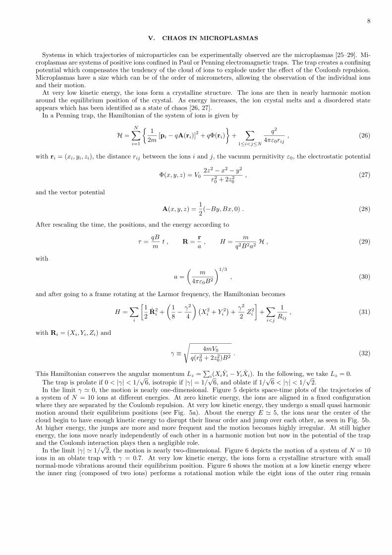
In the limit γ ' 0, the motion is nearly one-dimensional. Figure 5 depicts space-time plots of the trajectories ofa system of N = 10 ions at different energies. At zero kinetic energy, the ions are aligned in a fixed configurationwhere they are separated by the Coulomb repulsion. At very low kinetic energy, they undergo a small quasi harmonicmotion around their equilibrium positions (see Fig. 5a). About the energy E ' 5, the ions near the center of thecloud begin to have enough kinetic energy to disrupt their linear order and jump over each other, as seen in Fig. 5b.At higher energy, the jumps are more and more frequent and the motion becomes highly irregular. At still higherenergy, the ions move nearly independently of each other in a harmonic motion but now in the potential of the trapand the Coulomb interaction plays then a negligible role.

In the limit |γ| ' 1/√

2, the motion is nearly two-dimensional. Figure 6 depicts the motion of a system of N = 10ions in an oblate trap with γ = 0.7. At very low kinetic energy, the ions form a crystalline structure with smallnormal-mode vibrations around their equilibrium position. Figure 6 shows the motion at a low kinetic energy wherethe inner ring (composed of two ions) performs a rotational motion while the eight ions of the outer ring remain

9

-150

-100

-50

0

50

100

150

0 200 400 600 800 1000

spac

e Z

time

E = 4

(a)

-150

-100

-50

0

50

100

150

0 200 400 600 800 1000

spac

e Z

time

E = 5

(b)

-150

-100

-50

0

50

100

150

0 200 400 600 800 1000

spac

e Z

time

E = 10

(c)

-150

-100

-50

0

50

100

150

0 200 400 600 800 1000

spac

e Z

time

E = 20

(d)

FIG. 5: Space-time plots of the trajectories of a system of 10 ions in a prolate Penning trap with γ = 0.02 at total energies: (a)E = 4 with λ1 < 10−4 where the one-dimensional order is preserved; (b) E = 5 with λ1 ' 0.002 where an exchange betweentwo ions is observed at time τ ' 675 and Z ' −0.6; (c) E = 10 with λ1 ' 0.039 where exchanges are frequent; (d) E = 20with λ1 ' 0.045 where the harmonic motion of the ions in the trap potential becomes dominant. The kinetic energy of the ionsvanishes at the energy E0 = 3.444.

-15

-10

-5

0

5

10

15

-15 -10 -5 0 5 10 15

Y

X

E = 6.1(a)

-15

-10

-5

0

5

10

15

-15 -10 -5 0 5 10 15

Y

X

E = 6.5(b)

-15

-10

-5

0

5

10

15

-15 -10 -5 0 5 10 15

Y

X

E = 7(c)

FIG. 6: Space-time plots of the trajectories of a system of 10 ions in an oblate Penning trap with γ = 0.7 at total energies:(a) E = 6.1 with λ1 ' 0.003 where the ions have small-amplitude motion around the equilibrium positions of the ion crystal,except for the two ions in the inner which have an anti-clockwise rotational motion in a local mode; (b) E = 6.5 with λ1 ' 0.028where the ions jump between the inner and outer rings; (c) E = 7 with λ1 ' 0.041 where the ion crystal melts. The kineticenergy of the ions vanishes at the energy E0 = 6.087.

10

0

0.05

0.1

0.15

0.2

0.25

1 10 100 1000 10000

prolate

isotropic

oblate

Ly

apu

no

v e

xp

on

ent

E

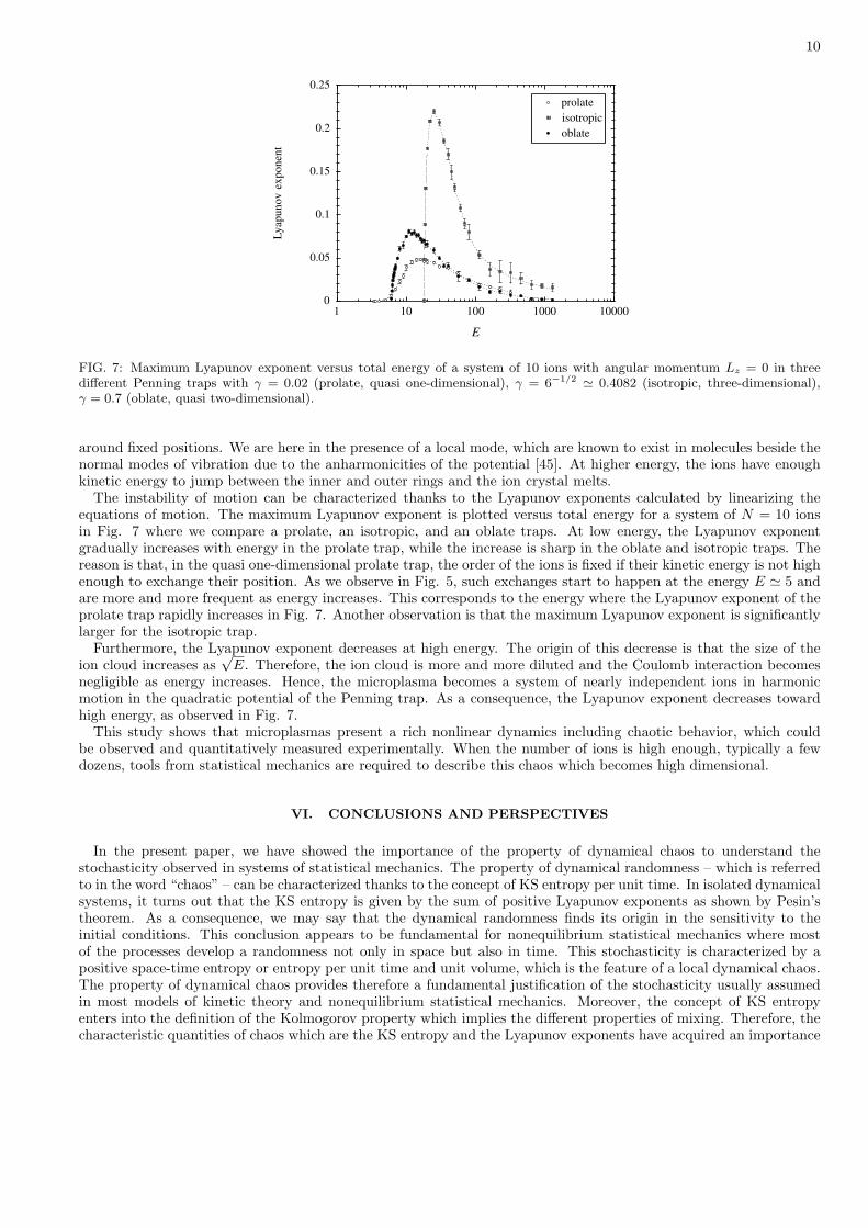
FIG. 7: Maximum Lyapunov exponent versus total energy of a system of 10 ions with angular momentum Lz = 0 in threedifferent Penning traps with γ = 0.02 (prolate, quasi one-dimensional), γ = 6−1/2 ' 0.4082 (isotropic, three-dimensional),γ = 0.7 (oblate, quasi two-dimensional).

around fixed positions. We are here in the presence of a local mode, which are known to exist in molecules beside thenormal modes of vibration due to the anharmonicities of the potential [45]. At higher energy, the ions have enoughkinetic energy to jump between the inner and outer rings and the ion crystal melts.

The instability of motion can be characterized thanks to the Lyapunov exponents calculated by linearizing theequations of motion. The maximum Lyapunov exponent is plotted versus total energy for a system of N = 10 ionsin Fig. 7 where we compare a prolate, an isotropic, and an oblate traps. At low energy, the Lyapunov exponentgradually increases with energy in the prolate trap, while the increase is sharp in the oblate and isotropic traps. Thereason is that, in the quasi one-dimensional prolate trap, the order of the ions is fixed if their kinetic energy is not highenough to exchange their position. As we observe in Fig. 5, such exchanges start to happen at the energy E ' 5 andare more and more frequent as energy increases. This corresponds to the energy where the Lyapunov exponent of theprolate trap rapidly increases in Fig. 7. Another observation is that the maximum Lyapunov exponent is significantlylarger for the isotropic trap.

Furthermore, the Lyapunov exponent decreases at high energy. The origin of this decrease is that the size of theion cloud increases as

√E. Therefore, the ion cloud is more and more diluted and the Coulomb interaction becomes

negligible as energy increases. Hence, the microplasma becomes a system of nearly independent ions in harmonicmotion in the quadratic potential of the Penning trap. As a consequence, the Lyapunov exponent decreases towardhigh energy, as observed in Fig. 7.

This study shows that microplasmas present a rich nonlinear dynamics including chaotic behavior, which couldbe observed and quantitatively measured experimentally. When the number of ions is high enough, typically a fewdozens, tools from statistical mechanics are required to describe this chaos which becomes high dimensional.

VI. CONCLUSIONS AND PERSPECTIVES

In the present paper, we have showed the importance of the property of dynamical chaos to understand thestochasticity observed in systems of statistical mechanics. The property of dynamical randomness – which is referredto in the word “chaos” – can be characterized thanks to the concept of KS entropy per unit time. In isolated dynamicalsystems, it turns out that the KS entropy is given by the sum of positive Lyapunov exponents as shown by Pesin’stheorem. As a consequence, we may say that the dynamical randomness finds its origin in the sensitivity to theinitial conditions. This conclusion appears to be fundamental for nonequilibrium statistical mechanics where mostof the processes develop a randomness not only in space but also in time. This stochasticity is characterized by apositive space-time entropy or entropy per unit time and unit volume, which is the feature of a local dynamical chaos.The property of dynamical chaos provides therefore a fundamental justification of the stochasticity usually assumedin most models of kinetic theory and nonequilibrium statistical mechanics. Moreover, the concept of KS entropyenters into the definition of the Kolmogorov property which implies the different properties of mixing. Therefore, thecharacteristic quantities of chaos which are the KS entropy and the Lyapunov exponents have acquired an importance

11

of their own and they deserve to be measured experimentally.In this perspective, we have considered in the present paper mesoscopic dynamical systems with several dozens

of particles, which are small enough for the methods of dynamical systems theory and large enough for those ofstatistical mechanics. In this regard, mesoscopic systems form the missing link between two fields of modern research:dynamical systems theory and nonequilibrium statistical mechanics or kinetic theory. Moreover, for these mesoscopicsystems, experimental techniques exist which allows the observation, on the one hand, of individual particles and theirtrajectories and, on the other hand, of collective properties currently studied in statistical mechanics. In particular,the observation of the trajectories allows the experimental measure of Lyapunov exponents by the Eckmann-Ruellealgorithm as well as the KS or ε-entropy per unit time thanks to the Grassberger-Procaccia algorithm [1].

Dynamical chaos is the common feature of Hamiltonian systems of particles in nonlinear interaction as shown herefor two types of systems: tracer or Brownian particles in a fluid of particles with short-range interactions such ashard balls and microplasmas of positive ions interacting with the long-range Coulomb force in Penning traps. Bothsystems present positive Lyapunov exponents.

In models of tracer or Brownian motion [24], the Lyapunov spectrum is dominated by Lyapunov exponents whichcan be associated with the tracer or Brownian particle in two regimes: (1) the Lorentz-gas regime with a tracerparticle lighter than the fluid particles and (2) the Rayleigh-flight regime in which the Brownian particle moves in anextremely rarified gas. The second regime is possible to be observed experimentally. The experimentally accessiblequantity is the ε-entropy per unit time of the Brownian particle and we may expect a cross-over in this quantity whichis similar to the cross-over in the Lyapunov spectrum.

In microplasmas, the study of the motion of ions and of its maximum Lyapunov exponent shows transitions as energyincreases. At very low kinetic energy, the microplasma condensates in an ion crystal and the ions have a vibrationalmotion of small amplitude around the equilibrium positions of the crystal. This motion is quasi harmonic and isa superposition of the normal modes of vibration. The anharmonicities and the maximum Lyapunov exponent aretherefore very small. Still at low kinetic energy, a transition may occur between a regime of normal-mode oscillationsto another with the excitation of some local modes (also called soft modes). In the present systems of ten ions, thislocal mode corresponds to the rotation of two ions with respect to the eight other ions. Such local modes are known inpolyatomic molecules [45] and it is remarkable to find that they are also the feature of ion crystals. At higher energy,the crystal melts and the motion becomes very chaotic. In this regime, the maximum Lyapunov exponent takes alarge positive value. This value is significantly higher for an isotropic trap than in the quasi one- and two-dimensionallimits. At even higher energy, the ions have large-amplitude oscillations in the harmonic potential of the Penningtrap. The energy in the Coulomb interaction becomes negligible hence the Lyapunov exponent decreases.

These results on Brownian motion in rarified gases and microplasmas are important predictions for future experi-ments on these systems.

Acknowledgments. The author thanks Professors J. R. Dorfman, G. Nicolis, and H. van Beijeren for supportand encouragement in this research. This research is financially supported by the FNRS Belgium as well as by theUniversite Libre de Bruxelles.

[1] J.-P. Eckmann and D. Ruelle, Rev. Mod. Phys. 57, 617 (1985).[2] P. Gaspard and G. Nicolis, Phys. Rev. Lett. 65, 1693 (1990).[3] D. J. Evans and G. Morriss, Statistical Mechanics of Nonequilibrium Liquids, (Academic Press, London, 1990).[4] N. I. Chernov, G. L. Eyink, J. L. Lebowitz, and Ya. G. Sinai, Phys. Rev. Lett. 70, 2209 (1993).[5] E. G. D. Cohen, Physica A 213, 293 (1995).[6] Ch. Dellago, H. A. Posch, and W. G. Hoover, Phys. Rev. E 53, 1485 (1996).[7] G. Gallavotti, Phys. Rev. Lett. 77, 4334 (1996).[8] P. Gaspard, Chaos, Scattering, and Statistical Mechanics (Cambridge University Press, Cambridge UK, 1998).[9] J. R. Dorfman, An Introduction to Chaos in Nonequilibrium Statistical Mechanics (Cambridge University Press, Cambridge

UK, 1999).[10] R. van Zon, H. van Beijeren, J. R. Dorfman, Kinetic Theory of Dynamical Systems, in: J. Karkheck, Editor, Dynamics:

Models and Kinetic Methods for Non-equilibrium Many-Body Systems (Kluwer, Dordrecht, 2000) pp. 131-167.[11] D. Ruelle, J. Stat. Phys. 95, 393 (1999).[12] D. Szasz, Editor, Hard Ball Systems and the Lorentz Gas, Encyclopaedia of Mathematical Sciences (Springer, Berlin, 2000).[13] J. R. Dorfman and P. Gaspard, Phys. Rev. E 51, 28 (1995).[14] P. Gaspard and J. R. Dorfman, Phys. Rev. E 52, 3525 (1995).[15] H. van Beijeren, A. Latz, and J. R. Dorfman, Phys. Rev. E 63, 016312 (2001).[16] T. Gilbert, J. R. Dorfman, and P. Gaspard, Nonlinearity 14, 339 (2001).[17] P. Gaspard, I. Claus, T. Gilbert, and J. R. Dorfman, Phys. Rev. Lett. 86, 1506 (2001).

12

[18] I. Claus and P. Gaspard, Physica D 168-169, 266 (2002).[19] H. van Beijeren and J. R. Dorfman, Phys. Rev. Lett. 74, 4412 (1995).[20] H. van Beijeren, J. R. Dorfman, H. A. Posch, and Ch. Dellago, Phys. Rev. E 56, 5272 (1997).[21] H. van Beijeren, A. Latz, and J. R. Dorfman, Phys. Rev. E 57, 4077 (1998).[22] R. van Zon, H. van Beijeren, and Ch. Dellago, Phys. Rev. Lett. 80, 2035 (1998).[23] J. R. Dorfman, A. Latz, and H. van Beijeren, Chaos 8, 444 (1998).[24] P. Gaspard and H. van Beijeren, J. Stat. Phys. 109, 671 (2002).[25] I. Siemers, R. Blatt, Th. Sauter, and W. Neuhauser, Phys. Rev. A 38, 5121 (1988).[26] J. Hoffnagle, R. G. DeVoe, L. Reyna, and R. G. Brewer, Phys. Rev. Lett. 61, 255 (1988).[27] R. Blumel, J. M. Chen, E. Peik, W. Quint, W. Schleich, Y. R. Shen, and H. Walther, Nature 334, 309 (1988).[28] L. R. Brewer, J. D. Prestage, J. J. Bollinger, W. M. Itano, D. J. Larson, and D. J. Wineland, Phys. Rev. A 38, 859 (1988).[29] M. G. Raizen, J. M. Gilligan, J. C. Bergquist, W. M. Itano, and D. J. Wineland, Phys. Rev. A 45, 6493 (1992).[30] M. S. Green, J. Chem. Phys. 22, 398 (1954).[31] R. Kubo, J. Phys. Soc. Jpn. 12, 570 (1957).[32] J.-P. Boon and S. Yip, Molecular Hydrodynamics (Dover, New York, 1980).[33] S. Mukamel, Principles of Nonlinear Optical Spectroscopy (Oxford University Press, New York, 1995).[34] I. P. Cornfeld, S. V. Fomin, and Ya. G. Sinai, Ergodic Theory (Springer-Verlag, Berlin, 1982).[35] S. Tasaki and P. Gaspard, J. Stat. Phys. 81, 935 (1995).[36] C. E. Shannon and W. Weaver, The Mathematical Theory of Communication (The University of Illinois Press, Urbana,

1949).[37] Ya. G. Sinai and N. I. Chernov, in: Ya. G. Sinai, Editor, Dynamical Systems: Collection of Papers (World Scientific,

Singapore, 1991) pp. 373-389.[38] H. Kantz and P. Grassberger, Physica D 17, 75 (1985).[39] N. G. van Kampen, Stochastic Processes in Physics and Chemistry (North-Holland, Amsterdam, 1981) pp. 358-364.[40] G. A. Bird, Phys. Fluids 6, 1518 (1963).[41] P. Gaspard and X.-J. Wang, Phys. Rep. 235, 291 (1993).[42] P. Gaspard and F. Baras, Phys. Rev. E 51, 5332 (1995).[43] I. Claus and P. Gaspard, Phys. Rev. E 63, 036227 (2001).[44] S. Viscardy and P. Gaspard, Viscosity in the escape-rate formalism: The case of two hard disks, preprint (2003).[45] P. van Ede van der Pals and P. Gaspard, J. Chem. Phys. 110, 5619 (1999).