introduction to survival analysis rich holubkov, ph.d. september 23, 2010

Introduction to Introduction to Survival AnalysisSurvival Analysis

Rich Holubkov, Ph.D.Rich Holubkov, Ph.D.

September 23, 2010September 23, 2010

Today’s ClassToday’s Class

• Introduction to, and motivation for, basic survival analysis techniques (and why we need advanced techniques)

• Presented at a “newbie Master’s statistician” level

• I will not assume you’ve seen survival data before, but necessarily will go through this material extremely quickly

• I do assume you know biostats basics like heuristics of chi-square statistics

Motivation for survival analysisMotivation for survival analysis

• Let’s say we have an event of interest, such as death or failure of a device.

• We may be interested in event rates at a particular timepoint (1 year), or assessing event rates over time as patients are being followed up.

• Could just calculate one-year rates…– Losses to follow-up before one year?– Patients not followed for one year as yet?– What if most events happen within 30

days?


• In studies where people are followed over a period of time, we usually have:– people in the study with different lengths

of follow-up (whether had event or not)– people dropping out of the study for

various reasons at different times

• We want to figure out rates of an event (like death, or liver transplant failure) at a particular time point (or all timepoints), taking this differential follow-up into account.


• We will often want to compare survival data between treatment groups (logrank test), quantify effects of factors on outcomes (Cox model and alternatives), sometimes in settings where patients can have competing outcomes (competing risks).

• Today, I will talk mainly about Kaplan-Meier curves and their comparison via logrank tests. No parametrics!

Motivating Example (briefly)Motivating Example (briefly)

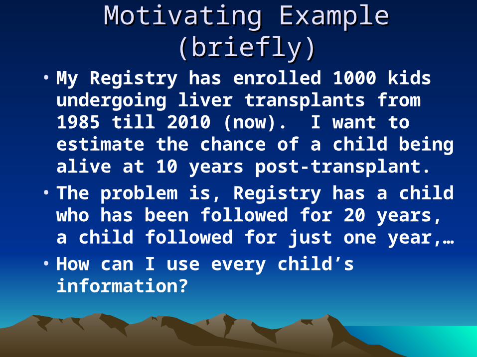
• My Registry has enrolled 1000 kids undergoing liver transplants from 1985 till 2010 (now). I want to estimate the chance of a child being alive at 10 years post-transplant.

• The problem is, Registry has a child who has been followed for 20 years, a child followed for just one year,…

• How can I use every child’s information?

Makes sense to look year by year!Makes sense to look year by year!(“Actuarial life tables”)(“Actuarial life tables”)

• I’ll see how many kids I had at the beginning of each year of follow-up(1000 enrolled in my Registry, 950 were around at beginning of two years, etc.)

• If a child dropped out of the analysis without dying (let’s say, during first year of follow-up, 25 withdrew or just weren’t around for long enough yet), makes sense to count that child as being around and “at risk” for half a year.

Actuarial Life TablesActuarial Life Tables

• Of my 1000 enrolled kids, at 1 year, 950 were alive, 25 dead, 25 dropouts/not followed long enough. 1-yr survival is:(950+12.5)/(950+25+12.5)=97.5%

• Examine the 950 left at beginning of Year 2 in same way. At end of 2 years, 900 were alive, 20 more dead, and 30 dropouts/not long enough. Additional 1-yr survival for these 950 is then(900+15)/(900+20+15)=97.9%.

• 2-yr survival=97.5% X 97.9%=95.4%

Extend this idea, event by event!Extend this idea, event by event!

• I can do this for 10 years, year by year.

• But, I can do this much more finely, effectively calculating an event rate at every timepoint where a child dies. Just need to know number left in the study (“at risk”) at each of those timepoints. This way of generating survival curves is called Kaplan-Meier analysis or the product-limit method.

A Kaplan-Meier ExampleA Kaplan-Meier Example http://www.cancerguide.org/scurve_km.html

Let’s say we have just seven patients:

Patient A: died at 1 yearPatient B: dropped out at 2 yearsPatient C: dropped out at 3 yearsPatient D: died at 4 yearsPatient E: still in study, alive at 5 yearsPatient F: died at 10 yearsPatient G: still in study, alive at 12 years

So, three deaths at 1, 4, and 10 years.

Kaplan-Meier calculationKaplan-Meier calculationhttp://www.cancerguide.org/scurve_km.html

Interval (Start-End)

# At Risk at Start of Interval

# Censored During Interval

# At Risk at End of Interval

# Who Died at End of Interval

Proportion Surviving at End of Interval

Cumulative Survival at End of Interval

0-1 7 0 7 1 6/7 = 0.86 0.86

1-4 6 2 4 1 3/4 = 0.75 0.86 * 0.75 = 0.64

4-10 3 1 2 1 1/2 = 0.5 0.86 * 0.75 * 0.5 = 0.31

10-12 1 0 1 0 1/1 = 1.0 0.86 * 0.75 * 0.5 * 1.0 = 0.31

This is our Kaplan-Meier curve!This is our Kaplan-Meier curve!

(It’s smoother if more observations)(It’s smoother if more observations)

For basic survival analysis, For basic survival analysis, we need for each patient:we need for each patient:

• A well-defined “time zero”, the date that follow-up begins

• A well-defined “date of event or last contact”, the last time we know if the patient had an event or not

• Above two elements are equivalent to “time on study”

• An indicator of whether or not the patient had an event at last contact.

Simple Analysis DatasetSimple Analysis Dataset

For our seven patient example:Event

TimeA: died at 1 year 1 1B: dropped out at 2 years 0 2C: dropped out at 3 years 0 3D: died at 4 years 1 4E: in study, alive at 5 years 0 5F: died at 10 years 1 10G: in study, alive at 12 years 0 12

Dropouts: a critical assumptionDropouts: a critical assumption

• Statistically: “any dropouts must be noninformative”. Dropout time should be independent of failure time.

• Practically: A child who drops out of the analysis cannot differ from a child who stays in analysis, in terms of chances of having an event as follow-up continues.

• Is this assumption ever reasonable?

• Is this assumption formally testable?

Simple ExampleSimple Example

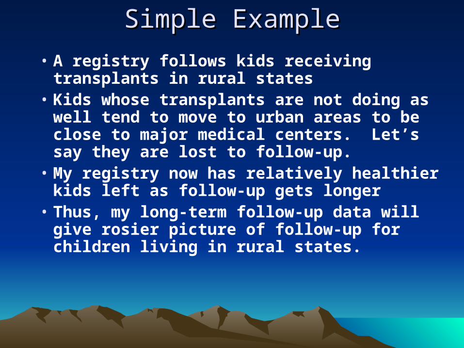
• A registry follows kids receiving transplants in rural states

• Kids whose transplants are not doing as well tend to move to urban areas to be close to major medical centers. Let’s say they are lost to follow-up.

• My registry now has relatively healthier kids left as follow-up gets longer

• Thus, my long-term follow-up data will give rosier picture of follow-up for children living in rural states.

A Variant…A Variant…• Recent improvements in surgical techniques/post-

surgical treatment have improved prognosis. So, kids transplanted decades ago have worse long-term prognosis. But, these are the only kids in my registry with long-term follow-up.

• So, my long-term follow-up data will give unnecessarily grim picture for recently treated kids. It’s just like healthy kids dropping out early!

• Changes in survival probability over time of enrollment is like nonrandom dropout.

A Variant I’ve SeenA Variant I’ve Seen

• A surgeon keeps his own registry. His research assistant regularly followed patients until about 5 years ago.

• He still regularly updates the registry database for important outcomes. Specifically, whenever he is notified that a patient has died, that patient’s survival data are updated.

• What will be wrong with the database for survival analysis?

• How can it be fixed?

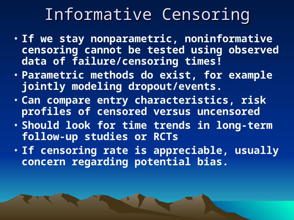
Informative CensoringInformative Censoring• If we stay nonparametric, noninformative

censoring cannot be tested using observed data of failure/censoring times!

• Parametric methods do exist, for example jointly modeling dropout/events.

• Can compare entry characteristics, risk profiles of censored versus uncensored

• Should look for time trends in long-term follow-up studies or RCTs

• If censoring rate is appreciable, usually concern regarding potential bias.

How can we compare How can we compare two (or more) survival curves?two (or more) survival curves?

• The standard approach to comparing survival curves between two or more groups, is termed the “logrank test”, sometimes known as the Mantel-Cox test.

• The test can be motivated in several ways. I present a “chi-squared table” approach, sort of like Mantel (1966).

How a logrank test works!How a logrank test works!

• At every timepoint when one or more kids have an event, we calculate the expected number of events in both groups assuming identical survival.

• If one child has event when there were 25 kids in Group A and 75 kids in Group B, we “expect” 0.25 events in Group A and 0.75 in Group B.

• Do this for all events, see if sum of the “Observed-Expected” for a group is large, like in the chi-squared test.

Heuristic DerivationHeuristic Derivation• j indexes times of events, 1 to J

• N1j, N2j number at risk at time j, Nj= N1j+N2j

• O1j, O2j # of events at time j, Oj= O1j+O2j

• Consider as 2 x 2 table for each time j:

Arm 1 Arm 2 Total

Dead O1j O2j Oj

Alive N1j-O1j N2j-O2j Nj-Oj

At Risk N1j N2j Nj


• If two arms truly have same survival distribution, then O1j is hypergeometric, so has expectation E1j =Oj(N1j/Nj) and variance V1j =(N1jN2jOj(Nj-Oj))/(Nj

2(Nj-1))

• Now get a statistic summing over the J event times, treating as sum of independent variables (this is very heuristic!!!)


• Under null, with E1j =Oj(N1j/Nj) and V1j =(N1jN2jOj(Nj-Oj))/(Nj

2(Nj-1)), (∑j(O1j-E1j ))2/∑jV1j has a chi-squared distribution with 1 d.f. This is the standard logrank test for testing equality between two survival curves.

• Readily generalizes to more than 2 groups, and to subgroups (strata) within each group to be compared.

Why this derivation?Why this derivation?

• Using our E1j =Oj(N1j/Nj) and V1j =(N1jN2jOj(Nj-Oj))/(Nj

2(Nj-1)), we can apply weights wj≡w(tj) at each event time tj, j=1,…,J. Then, the weighted statistic (∑j(wj(O1j -E1j ))2/∑jwjV1j still has a chi-squared distribution with 1 d.f.

• But, using wj ≡1 yields a test that is uniformly most powerful against all alternatives with proportional hazards (where “risk of event in Arm 1 vs. Arm 2” is constant throughout follow-up)

Why is this of interest?Why is this of interest?

• This is why we generally use a standard logrank (Mantel-Cox) test!

• But, programs like SAS will give or offer you other variants!– wj = Nj (Gehan-Wilcoxon or Breslow test, gives

more weight to earlier observations)

– wj = estimated proportion surviving at tj (Peto-Peto-Prentice Wilcoxon test, fully efficient for alternatives where odds ratio of event for Arm 2 vs. Arm 1 constant over time)

– There are classes of these test types…

Which test to use?Which test to use?

• For the practicing statistician, main thing is to be aware of these various test statistics and how they differ.

• We usually use the standard Mantel-Cox logrank test when planning a trial comparing survival curves, but whichever test is selected has to be prespecified.

• Can’t go hunting for significant p-values after an RCT. What about before?

Variance of Kaplan-Meier Variance of Kaplan-Meier EstimatesEstimates

• Using the delta method, if estimated survival at time t is S(t), an estimate of the variance of S(t) is S(t)2Σ(t

i<=t)Oi/((Ni-Oi)Ni).

• This estimate (Greenwood’s formula), used by SAS, is only modified at timepoints when events occur. Thus, estimated variance may not be proportional to subjects remaining at risk.

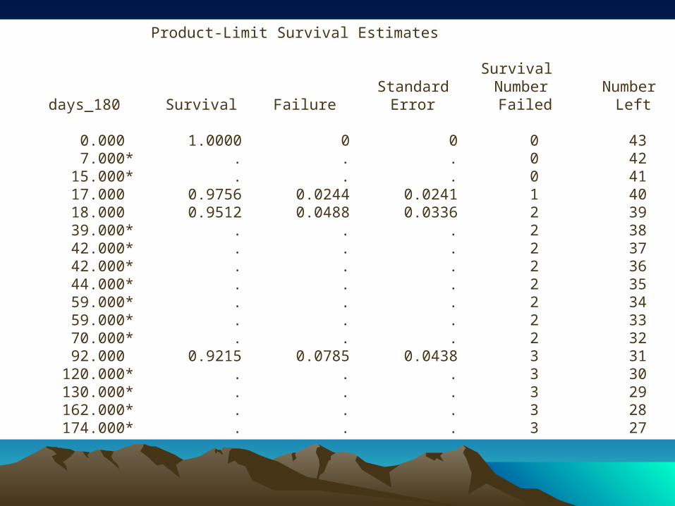
Product-Limit Survival Estimates

Survival Standard Number Number days_180 Survival Failure Error Failed Left

0.000 1.0000 0 0 0 43 7.000* . . . 0 42 15.000* . . . 0 41 17.000 0.9756 0.0244 0.0241 1 40 18.000 0.9512 0.0488 0.0336 2 39 39.000* . . . 2 38 42.000* . . . 2 37 42.000* . . . 2 36 44.000* . . . 2 35 59.000* . . . 2 34 59.000* . . . 2 33 70.000* . . . 2 32 92.000 0.9215 0.0785 0.0438 3 31 120.000* . . . 3 30 130.000* . . . 3 29 162.000* . . . 3 28 174.000* . . . 3 27


• You can implement Greenwood’s formula to get confidence intervals of a Kaplan-Meier rate at a particular timepoint, or to test hypotheses about that rate.

• Be aware that using the Kaplan-Meier nonparametric estimation approach will give substantially larger standard error estimates than parametrically based survival models.


• Peto (1977) derived alternative formula: if estimated survival at time t is S(t) and number at risk at time t is N(t), Peto estimate of the variance of S(t) is S(t)2[1-S(t)]/ N(t).

• Easy to compute, heuristically makes sense, perhaps(?) better when N smaller

• Worth knowing about and examining if testing an event rate is your primary goal!

• Neither great with N small/high censoring.

Interval CensoringInterval Censoring

• A patient dropping out of analysis before having an event is “right censored”.

• A patient who is known to have an event during some interval is called “interval censored”. For example, a cardiac echo on 12/1/2009 shows a valve leak. Previous echo was on 11/1/2008, and the leak could have started anytime between the two echos.

Left CensoringLeft Censoring• A patient who is known to have an event,

but not more specifically than before a particular date, is called “left censored”.

• For example (Klein/Moeschberger), a study looking at time till first marijuana use may have information from some kids who report use, but cannot recall the date at all.

• Special case of interval censoring.

Left Censoring (#1, #4)Left Censoring (#1, #4)


• Turnbull (1976) developed a nonparametric survival curve estimator applied to interval-censored data. Basically, an EM algorithm is used to compute the nonparametric MLE product-limit curve iteratively. Recently, more efficient algorithms have been developed to compute Kaplan-Meier type estimates.


• Just something to be aware of, if you encounter this type of data.

• SAS macros %EMICM and %ICSTEST allow construction of nonparametric survival curves with interval-censored data, and their comparison using a generalized version of the logrank test.

• R also has routines (“interval” package)

Curves with Interval CensoringCurves with Interval Censoring

Not a Pop Quiz, but…Not a Pop Quiz, but…

• A statistician familiar with survival basics may sometimes encounter data that didn’t turn out quite as expected.

• Here is an example I’ve certainly seen, though usually less extreme. I show hypothetical data on a six-month study with about 40 patients in each of two treatment groups…

What’s Your Conclusion? Why?What’s Your Conclusion? Why?

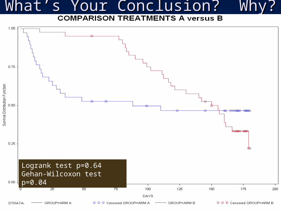
What’s Your Conclusion? Why?What’s Your Conclusion? Why?

Logrank test p=0.64Gehan-Wilcoxon test p=0.04

Crossing Curves ExampleCrossing Curves Example

• If this were a pilot observational study, logrank test is clearly inappropriate for a future trial if data are like this.

• Can consider a different test , shorter follow-up, or otherwise varying design of future trial, depending on setting (e.g., survival after cancer therapy)

• If these are results of an actual RCT with a prespecified logrank test, you are at least partly stuck.

Basic Survival Analysis in SASBasic Survival Analysis in SAS

• To do Kaplan-Meier and logrank in SAS:proc lifetest data=curves plots=s;time days*event(0);strata group;run;

• plots=s option asks for a Kaplan-Meier plot

• time statement: days is time on study,event is outcome indicator, with 0 as the value for patients who are censored (versus those who had an event).

• strata statement: compare levels of group

•

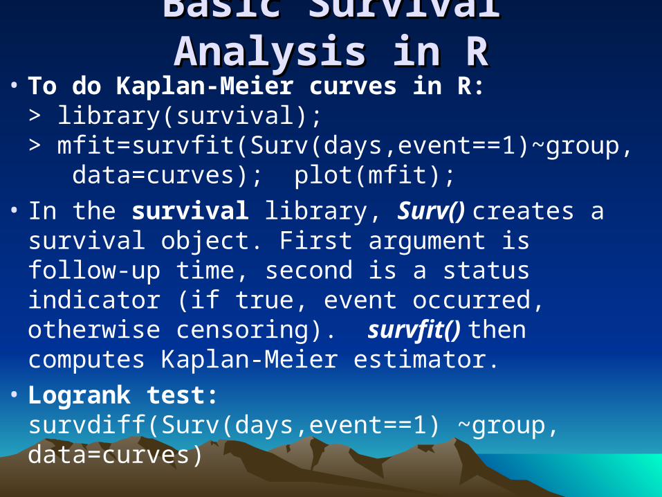
Basic Survival Analysis in RBasic Survival Analysis in R• To do Kaplan-Meier curves in R:

> library(survival);> mfit=survfit(Surv(days,event==1)~group, data=curves); plot(mfit);

• In the survival library, Surv() creates a survival object. First argument is follow-up time, second is a status indicator (if true, event occurred, otherwise censoring). survfit() then computes Kaplan-Meier estimator.

• Logrank test: survdiff(Surv(days,event==1) ~group, data=curves)

SummarySummary

• I have presented basic, nonparametric approaches to analysis of survival data. Kaplan-Meier curves and the logrank test should be a part of every biostatistician’s toolbox. Same is true for proportional hazards models, to be discussed next week by Nan Hu.

SummarySummary

• The survival analysis assumption of “noninformative censoring” usually cannot be formally tested and should be assumed not to hold. So, if a study has substantial dropout, there may be bias. Compare the characteristics of dropouts to others to get an idea of how bad the situation could be.

SummarySummary

• The usual logrank test can be viewed as just one member of a class of tests with different weightings of each event time. This test weights all event times equally, and is usually preferred as it’s uniformly most powerful when one treatment’s benefit (in terms of relative risk) is constant throughout follow-up. Variants may be preferred for nonstandard scenarios.

BibliographyBibliography• Fleming R, Harrington DP. Counting Processes and

Survival Analysis. 1991. Wiley.

• Kaplan EL, Meier P (1958). Nonparametric estimation from incomplete observations. JASA 53:457–481, 1958.

• Klein JP, Moeschberger ML. Survival Analysis: Techniques for Censored and Truncated Data. 2nd ed. 2003. Springer.

• Mantel, N (1966). Evaluation of survival data and two new rank order statistics arising in its consideration. Cancer Chemotherapy Reports 50(3): 163–70.

• Peto R, Pike MC, Armitage P, et al. (1977) Design and analysis of randomized clinical trials requiring prolonged observation of each patient, Part II. British Journal of Cancer 35: 1-39.

• Turnbull, B (1976). The empirical distribution function with arbitrarily grouped, censored and truncated data. JRSS-B, 38: 290-295.

Next SeminarNext Seminar

• Nan Hu, Ph.D. will be discussing the Cox proportional hazards model, one week from today on September 30th.

introduction to survival analysis rich holubkov, ph.d. september 23, 2010

Documents

year of followup

beginning of year

yr survival

year rates losses

event rates

survival data

child dies

differential followup