introduction to supervised ml concepts and algorithms
TRANSCRIPT

NBER Lectures on Machine Learning
An Introduction to Supervised
and Unsupervised Learning
July 18th, 2015, Cambridge
Susan Athey & Guido Imbens - Stanford University

Outline
1. Introduction
(a) Supervised Learning: Classification
(b) Supervised Learning: Regression
(c) Unsupervised Learning: Clustering
(d) Unsupervised Learning: Association Rules
2. Supervised Learning: Regression
(a) Linear Regression with Many Regressors: Ridge and
Lasso
1

(b) Regression Trees
(c) Boosting
(d) Bagging
(e) Random Forests
(f) Neural Networks and Deep Learning
(g) Ensemble Methods and Super Learners
3. Unsupervised Learning
(a) Principal Components
(b) Mixture Models and the EM Algorithm

(c) k-Means Algorithm
(d) Association Rules and the Apriori Algorithm
4. Classification: Support Vector Machines

1. Introduction
• Machine learning methods are about algorithms, more thanabout asymptotic statistical properties. No unified framework,like maximum likelihood estimation.
• “Does it work in practice?” rather than “What are its formalproperties?” Liberating, but also lack of discipline and lots ofpossibilities.
• Setting is one with large data sets, sometimes many units,sometimes many predictors. Scalability is a big issue
• Causality is de-emphasized. Methods are largely about pre-diction and fit. That is important in allowing validation ofmethods through out-of-sample crossvalidation.
• Lots of terminology, sometimes new terms for same things:“training” instead of “estimating”, etc.
2

Key Components
A. Out-of-sample Cross-validation: Methods are validated
by assessing their properties out of sample.
This is much easier for prediction problems than for causal
problems. For prediction problems we see realizations so that
a single observation can be used to estimate the quality of the
prediction: a single realization of (Yi, Xi) gives us an unbiased
estimate of µ(x) = E[Yi|Xi = x], namely Yi.
For causal problems we do not generally have unbiased esti-
mates of the true causal effects.
Use “training sample” to “train” (estimate) model, and “test
sample” to compare algorithms.
3

B. Regularization: Rather than simply choosing the best fit,there is some penalty to avoid over-fitting.
• Two issues: choosing the form of the regularization, andchoosing the amount of regularization.
Traditional methods in econometrics often used plug-in meth-ods: use the data to estimate the unknown functions and ex-press the optimal penalty term as a function of these quan-tities. For example, with nonparametric density estimation,researchers use the Silverman bandwith rule.
The machine learning literature has focused on out-of-samplecross-validation methods for choosing amount of regularization(value of penalty).
Sometimes there are multiple tuning parameters, and morestructure needs to be imposed on selection of tuning parame-ters.
4

C. Scalability: Methods that can handle large amounts of
data
• large number of units/observations and/or large number of
predictors/features/covariates) and perform repeatedly with-
out much supervision.
The number of units may run in the billions, and the number
of predictors may be in the millions.
The ability to parallelize problems is very important (map-
reduce).
Sometimes problems have few units, and many more predictors
than units: genome problems with genetic information for a
small number of individuals, but many genes.
5

1.a Supervised Learning: Classification
• One example of supervised learning is classification
• N observations on pairs (Yi, Xi), Yi is element of unordered
set {0,1, . . . , J}.
• Goal is to find a function g(x;X,Y) that assigns a new obser-
vation with XN+1 = x to one of the categories (less interest in
probabilities, more in actual assignment). XN+1 is draw from
same distribution as Xi, i = 1, . . . , N .
• Big success: automatic reading of zipcodes: classify each
handwritten digit into one of ten categories. No causality, pure
prediction. Modern problems: face recognition in pictures.
6

1.b Supervised Learning: Regression
• One example familiar from economic literature is nonpara-
metric regression: many cases where we need simply a
good fit for the conditional expectation.
• N observations on pairs (Yi, Xi). Goal is to find a function
g(x;X,Y) that is a good predictor for YN+1 for a new obser-
vation with XN+1 = x.
• Widely used methods in econometrics: kernel regression
g(x|X, Y) =N∑
i=1
Yi · K
(
Xi − x
h
)
/ N∑
i=1
K
(
Xi − x
h
)
Kernel regression is useful in some cases (e.g., regression dis-
continuity), but does not work well with high-dimensional x.
7

• Compared to econometric literature the machine learning
literature focuses less on asymptotic normality and properties,
more on out-of-sample crossvalidation.
• There are few methods for which inferential results have
been established. Possible that these can be established (e.g.,
random forests), but probably not for all, and not a priority in
this literature.
• Many supervised learning methods can be adapted to work
for classification and regression. Here I focus on estimating re-
gression functions because that is more familiar to economists.
8

2.a Linear Regression with Many Regressors: Ridge and
Lasso
Linear regression:
Yi =K∑
k=1
Xik · βk + εi = X′iβ + εi
We typically estimate β by ordinary least squares
β̂ols =
N∑
i=1
Xi · X′i
−1
N∑
i=1
Xi · Yi
=(
X′X
)−1 (X
′Y
)
This has good properties for estimating β given this model
(best linear unbiased estimator). But, these are limited op-
timality properties: with K ≥ 3 ols is not admissible. The
predictions x′β̂ need not be very good, especially with large K.
9

What to do with many covariates (large K)? (potentially
millions of covariates, and either many observations or modest
number of observations, e.g., genome data)
• Simple ols is not going to have good properties. (Like flat
prior in high-dimensional space for a Bayesian.)
Zvi Grilliches: “never trust ols with more than five regressors”
• We need some kind of regularization
Vapnik (of “support vector machines” fame): “Regularization
theory was one of the first signs of the existence of intelligent
inference”
10
Approaches to Regularization in Regression
• Shrink estimates continuously towards zero.
• Limit number of non-zero estimates: sparse representation.
“bet on the sparsity principle: use a procedure that does well
in sparse problems, since no procedure does well in dense prob-
lems” (Hastie, Tibshirani and Wainwright, 2015, p. 2)
• Combination of two
11
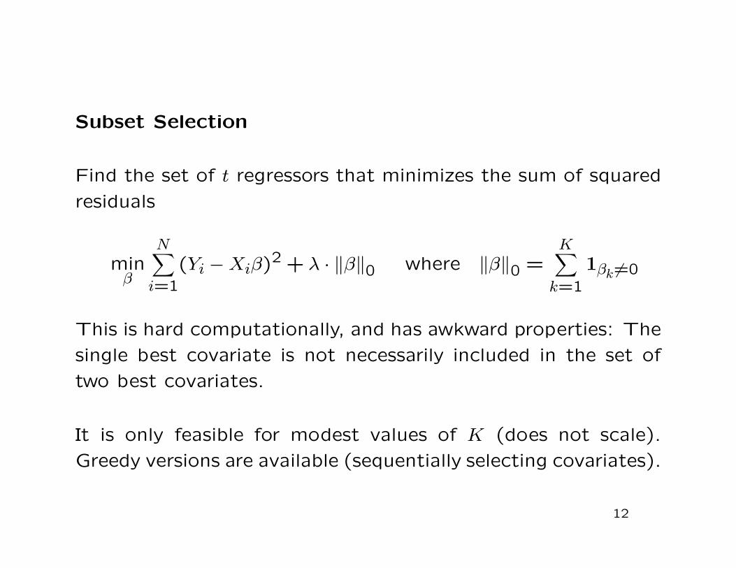
Subset Selection
Find the set of t regressors that minimizes the sum of squared
residuals
minβ
N∑
i=1
(Yi − Xiβ)2 + λ · ‖β‖0 where ‖β‖0 =K∑
k=1
1βk 6=0
This is hard computationally, and has awkward properties: The
single best covariate is not necessarily included in the set of
two best covariates.
It is only feasible for modest values of K (does not scale).
Greedy versions are available (sequentially selecting covariates).
12

Ridge Regression: Starting with the regression model
Yi =K∑
k=1
Xik · βk + εi = X′iβ + εi
We estimate β as
β̂ridge =(
X′X + λ · IK
)−1 (X
′Y
)
We inflate the X′X matrix by λ ·IK so that it is positive definite
irrespective of K, including K > N .
The solution has a nice interpretation: If the prior distribution
for β is N(0, τ2·IK), and the distribution of εi is normal N(0, σ2),
if λ = σ2/τ2, then β̂ridge is the posterior mean/mode/median.
The ols estimates are shrunk smoothly towards zero: if the Xikare orthonormal, all the ols coeffs shrink by a factor 1/(1+λ).
13

LASSO
“Least Absolute Selection and Shrinkage Operator” (Tibshi-
rani, 1996)
minβ
N∑
i=1
(Yi − Xiβ)2 + λ · ‖β‖1
This uses “L1” norm.
Lp norm is
‖x‖p =
K∑
k=1
|xk|p
1/p
Andrew Gelman: “Lasso is huge”
14

Compare L1 norm to L2 norm which leads to ridge:
β̂ridge = minβ
N∑
i=1
(Yi − Xiβ)2 + λ · ‖β‖22
Now all estimates are shrunk towards zero smoothly, no zero
estimates. This is easy computationally for modest K.
Or L0 norm leading to subset selection:
β̂subset = minβ
N∑
i=1
(Yi − Xiβ)2 + λ · ‖β‖0
Non-zero estimates are simple ols estimates. This is computa-
tionally challenging (combinatorial problem), but estimates are
interpretable.
16

beta ols0 0.1 0.2 0.3 0.4 0.5 0.6 0.7 0.8 0.9 1
beta
0
0.1
0.2
0.3
0.4
0.5
0.6
0.7
0.8
0.9
1best subset (- -), lasso (.-) and ridge (.) as function of ols estimates
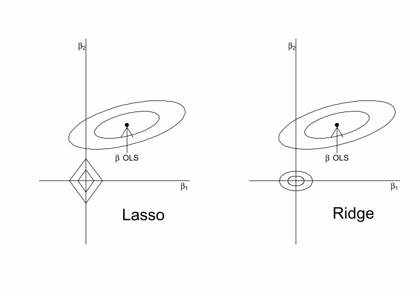
β1
β2
β OLS
Lasso
β1
β2
β OLS
Ridge

Related Methods
• LARS (Least Angle RegreSsion - “The ‘S’ suggesting LASSO
and Stagewise”) is a stagewise procedure that iteratively se-
lects regressors to be included in the regression function. It is
mainly used as an algorithm for calculating the LASSO coeffi-
cients as a function of the penalty parameter.
• Dantzig Selector (Candes & Tao, 2007)
minβ
Kmaxk=1
∣
∣
∣
∣
∣
∣
N∑
i=1
Xik · (Yi − Xiβ)
∣
∣
∣
∣
∣
∣
s.t. ‖β‖1 ≤ t
LASSO type regularization, but minimizing the maximum cor-
relation between residuals and covariates.
Interesting properties, but does not seem to work well for pre-
diction.
17

• LASSO is most popular of machine learning methods in
econometrics.
See Belloni, Chernozhukov, and Hansen Journal of Economic
Perspective, 2014 for general discussion and referencesto eco-
nomics literature.
18

What is special about LASSO?
LASSO shrinks some coefficients exactly to zero, and shrinks
the others towards zero.
(Minor modification is relaxed or post LASSO which uses LASSO
to selecte non-zero coefficients and then does simple ols on
those covariates without shrinking them towards zero.)
• Interpretability: few non-zero estimates, you can discuss
which covariates matter, unlike ridge.
• Good properties when the true model is sparse (bet on spar-
sity).
19

• No analytic solution, unlike ridge/L2 regression, but compu-
tationally attractive in very large data sets (convex optimiza-
tion problem) where X′X + λ · IK may be too large to invert.
• If we have a lot of regressors, what do we think the distri-
bution of the “true” parameter values is? Probably there are
some regressors that matter a lot, and a lot that matter very
little. Shrinking the large estimates a lot, as ridge does, may
not be effective.
• If the distribution of coefficients is very thick-tailed, LASSO
may do much better than ridge. On the other hand, if there
are a lot of modest size effects, ridge may do better. (see
discussion in original Tibshirani 1996 paper)
20

• Focus on covariate selection has awkward aspect. Consider
the case where we estimate a population mean by LASSO:
minµ
N∑
i=1
(Yi − µ)2 + λ · |µ|.
The estimate is zero if |Y | ≤ c, Y − c if Y > c, and Y + c if
Y < −c.
Relaxed LASSO here is zero if |Y | ≤ c, and Y if |Y | > c. This is
like a super-efficient estimator, which we typically do not like.
21

• Performance with highly correlated regressors is unstable.
Suppose Xi1 = Xi2, and suppose we try to estimate
Yi = β0 + β1 · Xi1 + β2 · Xi2 + εi.
Ridge regression would lead to β̂1 = β̂2 ≈ (β1 + β2)/2 (plus
some shrinkage).
Lasso would be indifferent between β̂1 = 0, β̂2 = β1 + β2 and
β̂1 = β1 + β2, β̂2 = 0.
22

LASSO as a Bayesian Estimator
We can also think of LASSO being the mode of the posterior
distribution, given a normal linear model and a prior distribution
that has a Laplace distribution
p(β) ∝ exp
−λ ·K∑
k=1
|βk|
• For a Bayesian using the posterior mode rather than the mean
is somewhat odd as a point estimate (but key to getting the
sparsity property, which generally does not hold for posterior
mean).
• Also it is less clear why one would want to use this prior
rather than a normal prior which would lead to an explicit form
for the posterior distribution.
23

• Related Bayesian Method: spike and slab prior.
In regression models we typically use normal prior distributions,
which are conjugate and have nice properties.
More in line with LASSO is to use a prior that is a mixture
of a distribution that has point mass at zero (the spike) and a
flatter component (the slab), say a normal distribution:
f(β) =
p if β = 0,
(1 − p) · 1(2πτ2)K/2 exp
(
−β′β2τ2
)
otherwise.
24

Implementation and Choosing the LASSO Penalty Pa-
rameter
We first standardize the Xi so that each component has mean
zero and unit variance. Same for Yi, so no need for intercept.
We can rewrite the problem
minβ
N∑
i=1
(Yi − Xiβ)2 + λ · ‖β‖1
as
minβ
N∑
i=1
(Yi − Xiβ)2 s.t.K∑
k=1
|βk| ≤ t ·K∑
k=1
|β̂olsk |
Now t is a scalar between 0 and 1, with 0 corresponding to
shrinking all estimates to 0, and 1 corresponding to no shrinking
and doing ols.
25

Typically we choose the penalty parameter λ (or t) through
crossvalidation. Let Ii ∈ {1, . . . , B} be an integer indicating the
B-th crossvalidation sample. (We could choose B = N to do
leave-one-out crossvalidation, but that would be computation-
ally difficult, so often we randomly select B = 10 crossvalida-
tion samples).
For crossvalidation sample b, for b = 1, . . . , B, estimate β̂b(λ)
β̂b(λ) = argminβ
∑
i:Ii 6=b
(Yi − Xiβ)2 + λ ·K∑
k=1
|βk|
on all data with Bi 6= b. Then calculate the sum of squared
errors for the data with Bi = b:
Q(b, λ) =∑
i:Ii=b
(
Yi − X′iβ̂b(λ)
)2
26
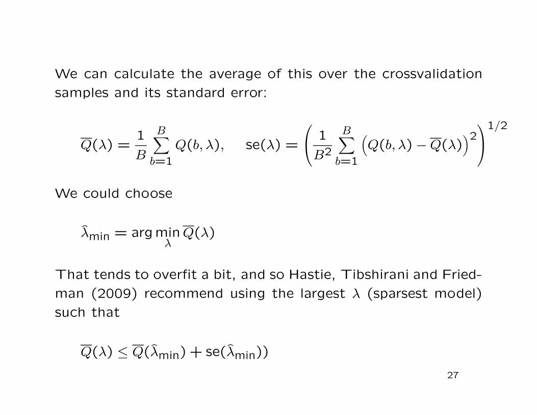
We can calculate the average of this over the crossvalidation
samples and its standard error:
Q(λ) =1
B
B∑
b=1
Q(b, λ), se(λ) =
1
B2
B∑
b=1
(
Q(b, λ) − Q(λ))2
1/2
We could choose
λ̂min = argminλ
Q(λ)
That tends to overfit a bit, and so Hastie, Tibshirani and Fried-
man (2009) recommend using the largest λ (sparsest model)
such that
Q(λ) ≤ Q(λ̂min) + se(λ̂min))
27

Oracle Property
If the true model is sparse, so that there are few (say, PN)
non-zero coefficients, and many (the remainder KN −PN) zero
coefficients, and PN goes to infinity slowly, whereas KN may
go to infinity fast (e.g., proportional to N), inference as if
you know a priori exactly which coefficients are zero is valid.
Sample size needs to be large relative to
PN ·
(
1 + ln
(
KN
PN
))
In that case you can ignore the selection of covariates part,
that is not relevant for the confidence intervals. This pro-
vides cover for ignoring the shrinkage and using regular
standard errors. Of course in practice it may affect the finite
sample properties substantially.
28

Example
Data on earnings in 1978 for 15,992 individuals. 8 features,
indicators for African-America, Hispanic, marital status, no-
degree, and continous variables age, education, earnings in
1974 and 1975. Created additional features by including all
interactions up to third order, leading to 121 features.
Training sample 7,996 individuals.
LASSO selects 15 out of 121 features, including 3 out of 8
main effects (education, earnings in 1974, earnings in 1975).
Test sample root-mean-squared error
OLS: 1.4093
LASSO: 0.7379
29


Elastic Nets
Combine L2 and L1 shrinkage:
minβ
N∑
i=1
(Yi − Xiβ)2 + λ ·(
α · ‖β‖1 + (1 − α) · ‖β‖22
)
Now we need to find two tuning parameters, the total amount
of shrinkage, λ, and the share of L1 and L2 shrinkage, captured
by α. Typically α is confined to a grid with few (e.g., 5) values.
30

2.b Nonparametric Regression: Regression Trees (Breiman,
Friedman, Olshen, & Stone, 1984)
• The idea is to partition the covariate space into subspaces
where the regression function is estimated as the average out-
come for units with covariate values in that subspace.
• The partitioning is sequential, one covariate at a time, always
to reduce the sum of squared deviations from the estimated
regression function as much as possible.
• Similar to adaptive nearest neighbor estimation.
31

Start with estimate g(x) = Y . The sum of squared deviations
is
Q(g) =N∑
i=1
(Yi − g(Xi))2 =
N∑
i=1
(
Yi − Y)2
For covariate k, for threshold t, consider splitting the data
depending on whether
Xi,k ≤ t versus Xi,k > t
Let the two averages be
Y left =
∑
i:Xi,k≤t Yi∑
i:Xi,k≤t 1Y right =
∑
i:Xi,k>t Yi∑
i:Xi,k>t 1
32

Define for covariate k and threshold t the estimator
gk,t(x) =
{
Y left if xk ≤ tY right if xk > t
Find the covariate k∗ and the threshold t∗ that solve
(k∗, t∗) = argmink,t
Q(gk,t(·))
Partition the covariate space into two subspaces, by whether
Xi,k∗ ≤ t∗ or not.
33

Repeat this, splitting the subspace that leads to the biggest
improvement in the objective function.
Keep splitting the subspaces to minimize the objective func-
tion, with a penalty for the number of splits (leaves):
Q(g) + λ · #(leaves)
• Result is flexible step function with properties that are difficult
to establish. No confidence intervals available.
34

Selecting the Penalty Term
To implement this we need to choose the penalty term λ for
the number of leaves.
We do essentially the same thing as in the LASSO case. Divide
the sample into B crossvalidation samples. Each time grow the
tree using the full sample excluding the b-th cross validation
sample, for all possible values for λ, call this g(b, λ). For each
λ sum up the squared errors over the crossvalidation sample to
get
Q(λ) =B∑
b=1
∑
i:Ii=b
(Yi − g(b, λ))2
Choose the λ that minimizes this criterion and estimate the
tree given this value for the penalty parameter. (Computational
tricks lead to focus on discrete set of λ.)
35

Pruning The Tree
Growing a tree this way may stop too early: splitting a particu-
lar leaf may not need to an improvement in the sum of squared
errors, but if we split anyway, we may find subsequently prof-
itable splits.
For example, suppose that there are two binary covariates,
Xi1, Xi,2 ∈ {0,1}, and that
E[Yi|Xi,1 = 0,Xi,2 = 0] = E[Yi|Xi,1 = 1, Xi,2 = 1] = −1
E[Yi|Xi,1 = 0,Xi,2 = 1] = E[Yi|Xi,1 = 0, Xi,2 = 1] = 1
Then splitting on Xi1 or Xi2 does not improve the objective
function, but once one splits on either of them, the subsequent
splits lead to an improvement.
36
This motivates pruning the tree:
• First grow a big tree by using a deliberately small value of the
penalty term, or simply growing the tree till the leaves have a
preset small number of observations.
• Then go back and prune branches or leaves that do not
collectively improve the objective function sufficiently.
37
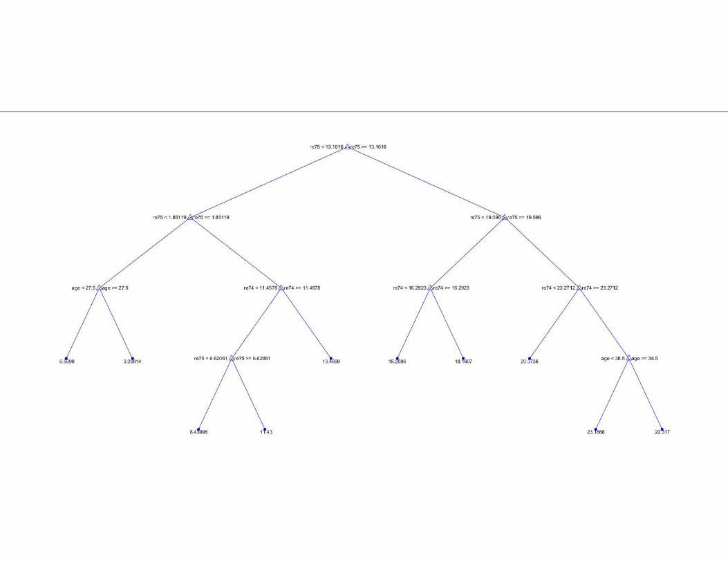

Tree leads to 37 splits
Test sample root-mean-squared error
OLS: 1.4093
LASSO: 0.7379
Tree: 0.7865
38


2.c Boosting
Suppose we have a simple, possibly naive, but easy to com-
pute, way of estimating a regression function, a so-called weak
learner.
Boosting is a general approach to repeatedly use the weak
learner to get a good predictor for both classification and re-
gression problems. It can be used with many different weak
learners, trees, kernels, support vector machines, neural net-
works, etc.
Here I illustrate it using regression trees.
39

Suppose g(x|X, Y) is based on a very simple regression tree,
using only a single split. So, the algorithm selects a covari-
ate k(X,Y) and a threshold t(X,Y) and then estimates the
regression function as
g1(x|X, Y) =
{
Y left if xk(X,Y) ≤ t(X,Y)
Y right if xk(X,Y) > t(X,Y)
where
Y left =
∑
i:Xi,k≤t Yi∑
i:Xi,k≤t 1Y right =
∑
i:Xi,k>t Yi∑
i:Xi,k>t 1
Not a very good predictor by itself.
40

Define the residual relative to this weak learner:
ε1i = Yi − g1(Xi|X, Y)
Now apply the same weak learner to the new data set (X, ε1).
Grow a second tree g2(X, ε1) based on this data set (with single
split), and define the new residuals as
ε2i = Yi − g1(Xi|X, Y) − g2(Xi|X, ε1)
Re-apply the weak learner to the data set (X, ε2).
After doing this many times you get an additive approximation
to the regression function:
M∑
m=1
gm(x|X, εm−1) =K∑
k=1
hk(xk) where ε0 = Y
41
Had we used a weak learner with two splits, we would have
allowed for second order effects h(xk, xl).
In practice researchers use shallow trees, say with six splits
(implicitly allowing for 6-th order interactions), and grow many
trees, e.g., 400-500.
Often the depth of the initial trees is fixed in advance in an ad
hoc manner (difficult to choose too many tuning parameters
optimally), and the number of trees is based on prediction
errors in a test sample (similar in spirit to cross-validation).
42

2.d Bagging (Bootstrap AGGregatING) Applicable to manyways of estimating regression function, here applied to trees.
1. Draw a bootstrap sample of size N from the data.
2. Construct a tree gb(x), possibly with pruning, possibly withdata-dependent penalty term.
Estimate the regression function by averaging over bootstrapestimates:
1
B
B∑
b=1
gb(x)
If the basic learner were linear, than the bagging is ineffective.For nonlinear learners, however, this smoothes things and canlead to improvements.
43

2.e Random Forests (Great general purpose method)
Given data (X,Y), with the dimension of X equal to N ×K, dothe same as bagging, but with a different way of constructingthe tree given the bootstrap sample: Start with a tree with asingle leaf.
1. Randomly select L regressors out of the set of K regressors
2. Select the optimal cov and threshold among L regressors
3. If some leaves have more than Nmin units, go back to (1)
4. Otherwise, stop
Average trees over bootstrap samples.
44

• For bagging and random forest there is recent research sug-
gesting asymptotic normality may hold. It would require using
small training samples relative to the overall sample (on the
order of N/(ln(N)K), where K is the number of features.
See Wager, Efron, and Hastie (2014) and Wager (2015).
45

2.f Neural Networks / Deep Learning
Goes back to 1990’s, work by Hal White. Recent resurgence.
Model the relation between Xi and Yi through hidden layer(s)
of Zi, with M elements Zi,m:
Zi,m = σ(α0m + α′1mXi), for m = 1, . . . , M
Yi = β0 + β′1Zi + εi
So, the Yi are linear in a number of transformations of the
original covariates Xi. Often the transformations are sigmoid
functions σ(a) = (1 + exp(−a))−1. We fit the parameters αm
and β by minimizing
N∑
i=1
(Yi − g(Xi, α, β))2
46

• Estimation can be hard. Start with α random but close to
zero, so close to linear model, using gradient descent methods.
• Difficulty is to avoid overfitting. We can add a penalty term
N∑
i=1
(Yi − g(Xi, α, β))2 + λ ·
∑
k,m
α2k,m +
∑
k
β2k
Find optimal penalty term λ by monitoring sum of squared
prediction errors on test sample.
47
2.g Ensemble Methods, Model Averaging, and Super Learn-
ers
Suppose we have M candidate estimators gm(·|X, Y). They can
be similar, e.g., all trees, or they can be qualitatively different,
some trees, some regression models, some support vector ma-
chines, some neural networks. We can try to combine them to
get a better estimator, often better than any single algorithm.
Note that we do not attempt to select a single method, rather
we look for weights that may be non-zero for multiple methods.
Most competitions for supervised learning methods have been
won by algorithms that combine more basic methods, often
many different methods.
48

One question is how exactly to combine methods.
One approach is to construct weights α1, . . . , αM by solving,using a test sample
minα1,...,αM
N∑
i=1
Yi −M∑
m=1
αm · gm(Xi)
2
If we have many algorithms to choose from we may wish toregularize this problem by adding a LASSO-type penalty term:
λ ·M∑
m=1
|αm|
That is, we restrict the ensemble estimator to be a weightedaverage of the original estimators where we shrink the weights
using an L1 norm. The result will be a weighted average thatputs non-zero weights on only a few models.
49

Test sample root-mean-squared error
OLS: 1.4093
LASSO: 0.7379
Tree: 0.7865
Ensemble: 0.7375
Weights ensemble:
OLS 0.0130
LASSO 0.7249
Tree 0.2621
50

3. Unsupervised Learning: Clustering
We have N observations on a M-component vector of features,
Xi, i = 1, . . . , N . We want to find patterns in these data.
Note: there is no outcome Yi here, which gave rise to the term
“unsupervised learning.”
• One approach is to reduce the dimension of the Xi using
principal components. We can then fit models using those
principal components rather than the full set of features.
• Second approach is to partition the space into a finite set.
We can then fit models to the subpopulations in each of those
sets.
51

3.a Principal Components
• Old method, e.g., in Theil (Principles of Econometrics)
We want to find a set of K N-vectors Y1, . . . , YK so that
Xi ≈K∑
k=1
γikYk
or, collectively, we want to find approximation
X = ΓY, Γ is M × K, M > K
This is useful in cases where we have many features and we
want to reduce the dimension without giving up a lot of infor-
mation.
52
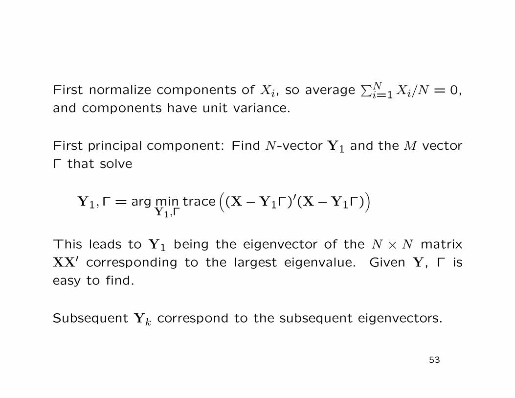
First normalize components of Xi, so average∑N
i=1 Xi/N = 0,
and components have unit variance.
First principal component: Find N-vector Y1 and the M vector
Γ that solve
Y1, Γ = arg minY1,Γ
trace(
(X − Y1Γ)′(X − Y1Γ))
This leads to Y1 being the eigenvector of the N × N matrix
XX′ corresponding to the largest eigenvalue. Given Y, Γ is
easy to find.
Subsequent Yk correspond to the subsequent eigenvectors.
53

3.b Mixture Models and the EM Algorithm
Model the joint distribution of the L-component vector Xi as
a mixture of parametric distributions:
f(x) =K∑
k=1
πk · fk(x; θk) fk(·; ·) known
We want to estimate the parameters of the mixture compo-
nents, θk, and the mixture probabilities πk.
The mixture components can be multivariate normal, of any
other parametric distribution. Straight maximum likelihood
estimation is very difficult because the likelihood function is
multi-modal.
54

The EM algorithm (Dempster, Laird, Rubin, 1977) makes this
easy as long as it is easy to estimate the θk given data from
the k-th mixture component. Start with πk = 1/K for all k.
Create starting values for θk, all different.
Update weights, the conditional probability of belonging to
cluster k given parameter values (E-step in EM):
wik =πk · fk(Xi; θk)
∑Km=1 πm · fm(Xi; θm)
Update θk (M-step in EM)
θk = argmaxθ
N∑
i=1
wik · ln fk(Xi; θ)
55
Algorithm can be slow but is very reliable. It gives probabilities
for each cluster. Then we can use those to assign new units
to clusters, using the highest probability.
Used in duration models in Gamma-Weibull mixtures (Lan-
caster, 1979), non-parametric Weibull mixtures (Heckman &
Singer, 1984).
56

3.c The k-means Algorithm
1. Start with k arbitrary centroids cm for the k clusters.
2. Assign each observation to the nearest centroid:
Ii = m if ‖Xi − cm‖ = minm′=1
‖Xi − cm′‖
3. Re-calculate the centroids as
cm =∑
i:Ii=m
Xi
/
∑
i:Ii=m
1
4. Go back to (2) if centroids have changed, otherwise stop.
57
• k-means is fast
• Results can be sensitive to starting values for centroids.
58

3.d. Mining for Association Rules: The Apriori Algorithm
Suppose we have a set of N customers, each buying arbitrary
subsets of a set F0 containing M items. We want to find
subsets of k items that are bought together by at least L cus-
tomers, for different values of k.
This is very much a data mining exercise. There is no model,
simply a search for items that go together. Of course this
may suggest causal relationships, and suggest that discounting
some items may increase sales of other items.
It is potentially difficult, because there are M choose k subsets
of k items that could be elements of Fk. The solution is to do
this sequentially.
59

You start with k = 1, by selecting all items that are bought
by at least L customers. This gives a set F1 ⊂ F0 of the M
original items.
Now, for k ≥ 2, given Fk−1, find Fk.
First construct the set of possible elements of Fk. For a set
of items F to be in Fk, it must be that any set obtained by
dropping one of the k items in F , say the m-th item, leading
to the set F(m) = F/{m}, must be an element of Fk−1.
The reason is that for F to be in Fk, it must be that there
are at least L customers buying that set of items. Hence there
must be at least L customers buying the set F(m), and so F(m)
is an k − 1 item set that must be an element of Fk−1.
60

5. Support Vector Machines and Classification
Suppose we have a sample (Yi, Xi), i = 1, . . . , N , with Yi ∈
{−1,1}.
We are trying to come up with a classification rule that assigns
units to one of the two classes −1 or 1.
One conventional econometric approach is to estimate a logis-
tic regression model and assign units to the groups based on
the estimated probability.
Support vector machines look for a boundary h(x), such that
units on one side of the boundary are assigned to one group,
and units on the other side are assigned to the other group.
61
Suppose we limit ourselves to linear rules,
h(x) = β0 + xβ1,
where we assign a unit with features x to class 1 if h(x) ≥ 0
and to -1 otherwise.
We want to choose β0 and β1 to optimize the classification.
The question is how to quantify the quality of the classification.
62

Suppose there is a hyperplane that completely separates the
Yi = −1 and Yi = 1 groups. In that case we can look for the
β, such that ‖β‖ = 1, that maximize the margin M :
maxβ0,β1
M s.t. Yi · (β0 + Xiβ1) ≥ M ∀i, ‖β‖ = 1
The restriction implies that each point is at least a distance M
away from the boundary.
We can rewrite this as
minβ0,β1
‖β‖ s.t. Yi · (β0 + Xiβ1) ≥ 1 ∀i.
63

Often there is no such hyperplane. In that case we define a
penalty we pay for observations that are not at least a distance
M away from the boundary.
minβ0,β1
‖β‖ s.t. Yi · (β0 + Xiβ1) ≥ 1 − εi, εi ≥ 0 ∀i,∑
i
ε ≤ C.
Alternatively
minβ
1
2· ‖β‖ + C ·
∑
i=1
εi
subject to
εi ≥ 0, Yi · (β0 + Xiβ1) ≥ 1 − εi
64
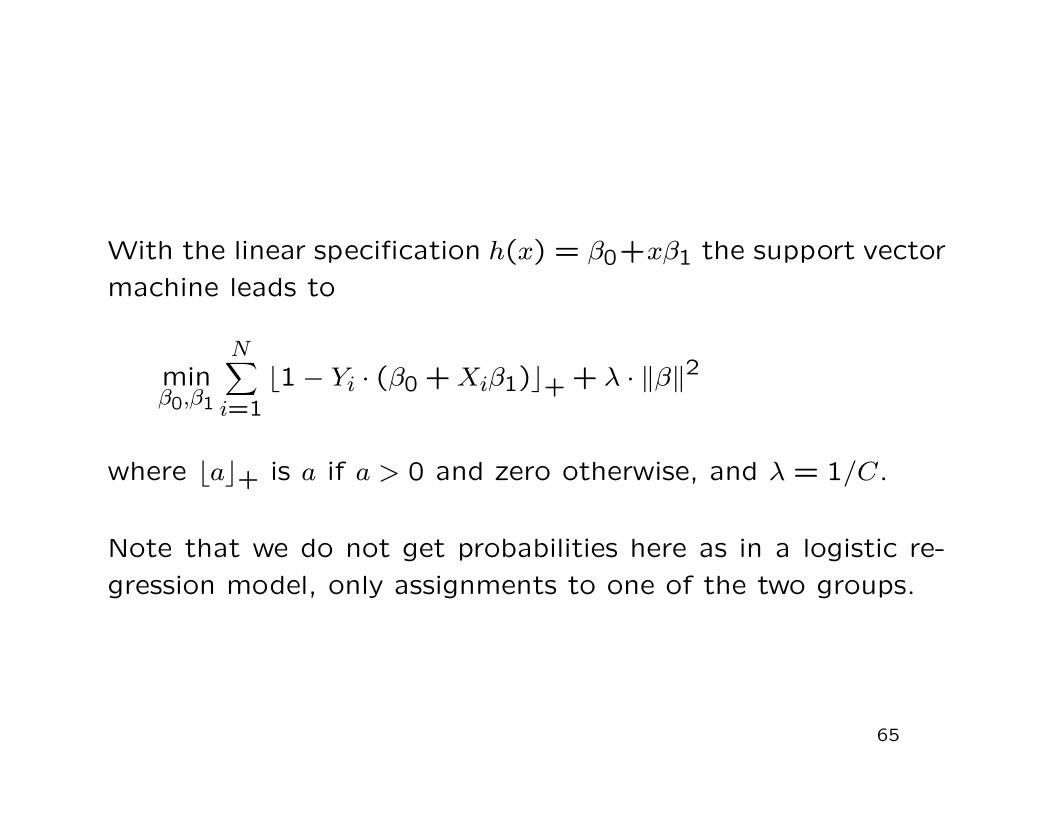
With the linear specification h(x) = β0+xβ1 the support vector
machine leads to
minβ0,β1
N∑
i=1
b1 − Yi · (β0 + Xiβ1)c+ + λ · ‖β‖2
where bac+ is a if a > 0 and zero otherwise, and λ = 1/C.
Note that we do not get probabilities here as in a logistic re-
gression model, only assignments to one of the two groups.
65

Thank You!
66