195

Introduction to Statistics and Hypothesis Testing Overview We will be using some basic statistics this semester. Because a statistics class is not a required prerequisite for this course, we are going to use the first lab to go over and practice applying some very basic statistical concepts. You will use these concepts repeatedly in your lab write-ups and for your Student-Driven Independent Projects. This abridged statistics manual is organized into three sections: I) An introduction to hypothesis testing. II) An introduction to statistical concepts, and in what settings to apply them. At the end of this section you will find a summary table and a flow chart that may help you decide in which setting to use a particular statistical test. III) The last section provides the mathematical procedures for each of the introduced statistical concepts, and (where applicable) how to run each test using excel. Terms in bold are terms you should know the definitions of. References Modified from Cáceres, C.E. 2007. IB 449, Limnology Lab Manual. Modified from Augspurger, C.K. and G.O. Batzli. 2008. IB 203, Exercises in Ecology Course Manual.

196

I) Introduction to Hypothesis Testing Asking questions in a scientifically meaningful way Statistics are of little use unless you first have a clear hypothesis and a specific quantitative prediction to test. Consider a simple example. You are interested in the research question whether herbivores affect the amount of algae present in lake water. You make that speculation a bit more specific and develop a general hypothesis: The presence of herbivores reduces the abundance of algae in lake water. Now you have something to work with, but it is still a pretty vague notion. What you need to do is apply this hypothesis to a specific study system. You know from surveys of local lakes that some lakes have Daphnia (large herbivorous zooplankton) whereas others do not. So, based on your hypothesis, you can now make a specific, testable prediction: The mean abundance of algae will be greater in lakes without Daphnia than in lakes where Daphnia are present. The hypothesis and its prediction can be formally written as an if-then statement as follows: If herbivores affect the amount of algae in lake water, then the mean abundance of algae will be greater in lakes without Daphnia than in lakes with Daphnia. Once you have a quantitative prediction firmly in mind for your experiment or study system, you can proceed to the next step – forming statistical hypotheses for testing. Statistical hypotheses are possible quantitative relationships among means or associations among variables. The null hypothesis (Ho) states that there is no association among two variables, or no difference among means. For our example, it would be stated as “Ho: algal abundance in Daphnia-absent lakes = algal abundance in Daphnia-present lakes” (or, Ho: A = B). The alternative hypothesis (H1) states the pattern in the data that is expected if your predictions hold true. For our example, “H1: algal abundance in Daphnia-absent lakes > algal abundance in Daphnia-present lakes” (or, H1: A > B). Once our question has taken on this shape, we can begin thinking about experimental design, and start collecting data. Answering your questions Now you have to go out, collect data, and evaluate whether or not the data support your hypothesis. Ideally, we might want to know the mean abundance of algae in ALL lakes with and without Daphnia, a population of lakes that would constitute the universal set. However, this is rarely if ever feasible or possible. Instead, we are usually restricted to pick a subset of lakes (a sample set, or sample in short) from each type of lake, which allows us to obtain an estimate of the overall relationship between algal abundance and Daphnia presence of the universal set. Hopefully, the sample set is representative of the universal set. Selecting unbiased, random methods of sampling can go a long way in ensuring that the sample set has a greater likelihood of being representative of the

197

universal set. We will explore sampling strategies in Lab 3 and on the upcoming field trip to southern Illinois. Because our sample set represents merely an estimate of the universal set, inevitably one group’s mean WILL be higher than the other’s, even if there is no difference in means in the universal set, just by random chance! Repeat the last sentence 10 times. If you don’t understand why we asked you to repeat that sentence, ASK, this is a key aspect of the entire course. After you have collected your data and calculated your two means (Daphnia-absent, Daphnia-present), you notice that the mean for the Daphnia-absent group appears to be higher than the mean for the Daphnia-present group. That’s nice, but it doesn’t tell us much. As we just got through saying 10 times over, one or the other group’s mean was going to be greater even if only by random chance. Our problem is to decide, based on the data, whether the difference we observed was likely to be caused by chance alone or whether we can conclude that there probably is some real difference between the two groups. Statistics help us make this decision by assigning p-values to tests for differences between means. P-values range between 0 (impossible for difference to be due to chance) and 1 (certain that difference is due to chance). They can be thought of as the probability that the differences among means observed were caused by chance variation. If the p-value is very small (traditionally, and for this class, < 0.05), you conclude that there is some systematic difference between the means. You have measured a difference that was probably NOT caused by chance. “Something else” (maybe grazing by Daphnia?) is going on. You reject the null hypothesis (Ho: A = B) and claim evidence for the alternative hypothesis (H1: A > B); algal abundance was significantly greater in the Daphnia-absent lakes than in the Daphnia-present lakes. If, on the other hand, the p-value is > 0.05 there is a good chance that, if you tried the experiment again with two new samples of lakes, you would have gotten the opposite result. You have to accept the null hypothesis. You really have no strong evidence for a difference in algal abundance between the two groups of lakes.

198

II) Introduction to Statistical Concepts In this section we cover three main topics:

A) What type of variable are you dealing with in your experiment (the selection of the statistical test will partly depend on your type of variable).

B) Univariate Statistics (also called Descriptive Statistics), which helps you to describe attributes of individual variables of your data set.

C) Analytical Statistics, which allows you to test for differences or relationships between variables.

A) Types of Variables

There are three types of variables: discrete, continuous, and categorical.

Discrete variables are those that cannot be subdivided. They must be a whole number. E.g. cats would be discrete data because there cannot be a fraction of a cat. We count or tally these data.

Continuous variables are those values that cover an uninterrupted range of scales. A good example of a continuous variable is pH, temperature or height. Categorical variables are arbitrarily assigned by the experimenter. An example of a categorical variable is an experiment with two treatments: you supplement a certain number of plants with nitrogen (treatment 1), and another number of plants get no nitrogen (treatment 2). So your categorical variable has two levels: nitrogen and no nitrogen. Note that categorical variables have distinct, mutually exclusive categories that lack quantitative intermediaries (e.g. present vs. absent; orange vs. green vs. brown plumage).

Each of these three variable types can either be an independent or a dependent variable. Consider the following example: We have data on light intensity and algal biomass for twenty locations within a reach of stream. We suspect that higher light intensities may lead to more algal biomass. That sentence assumes directionality in the relationship of the two variables. Light intensity is suspected to influence algal biomass, not the other way around. So light is independent, whereas algal biomass is dependent on light intensity. Another way of thinking about this is that the independent variable is the variable manipulated by us during the experiment (light) to test the response in the dependent variable (algal biomass). We are not likely to try to manipulate algal biomass and expect the light intensity striking the water surface to change as a result.

Distinguishing between a dependent and an independent variable is important for calculating several statistical tests, so it is important that you become familiar with this distinction.

199

B) Descriptive Statistics (Univariate Statistics) If we take the time to closely investigate any biological species or phenomenon we will find that variation is the norm, not the exception. If we are to describe a particular characteristic of a species for example, it thus does not suffice to choose a “perfect specimen” to measure. One of Charles Darwin's great insights was to realize that for species the interesting thing was the variation within a population, the spread, and not the population mean or a representative abstraction (the Platonic ideal or holotype). Variation - the deviations from the mean - can play a critical role in understanding a natural system. There are several commonly used descriptive statistics to use on discrete and continuous variables. These include measures of central tendency, measures of dispersion, and measures of symmetry and shape. A brief description of the most important of each of these follows below. Histograms as an exploratory tool A good starting point to understanding the variation in a data set is to determine the distribution of values of the measured variable. A distribution is a mathematical map of how the frequency of occurrence changes as a function of variable magnitude. The best way to see and first investigate the distribution is by the construction of a histogram. The x-axis is the variable value (e.g. size), and the y-axis is a measure of the frequency that a variable or range of variables occurs. A histogram gives you a quick, first visual impression of the data you collected. The shape of the distribution that we plotted as a histogram can be described in terms of three categories: descriptors of central tendency, of dispersion, and of symmetry. The following description applies mainly to unimodal distributions (distributions with only one peak). Bimodal or polymodal distributions often (but not always) imply that the sample set consists of more than one population, and the sampling scheme may have to be rethought

Measures of central tendency

mode: most frequently occurring value (highest peak of the frequency distribution)

median: # such that half the values are lower and half are higher.

arithmetic mean: a.k.a. the average. The sum of all the values (xi) divided by the number of data points (n):

!

x = (!xi)/n = (x1 + x2 + x3 + … + xi)/n

200

Measures of dispersion range: the difference between the maximum and minimum value: xmax - xmin variance: the average of the squared deviations from the mean in a sample or

population. The variance considers how far each point is from the mean. The variance for a population (the universal set) is denoted by !" and is calculated as:

!

2" =

populationSSN

WHERE: SS = Sum of Squares =

!

xi " x# $

% & '2

The best estimate of the population variance is the sample variance, s2:

s2 =

!

sampleSSn "1

standard deviation = square root of the variance [st. dev. = ! = #(!")]. The

standard deviation is a description of the spread of data points around the mean. An approximate way to think about the standard deviation is as an average of the amount that the observations deviate from the mean. If the observations form a normal distribution (see below) around the mean, and ONLY if they form a normal distribution, 68% of the observations are within +/- 1 standard deviation, 95.4% of the observations are within +/- 2 standard deviations, and 99.7% of the observations are within +/- 3 standard deviations of the mean.

standard error: The standard error is defined at the standard deviation divided

by the square root of the number of observations, or: SE = standard deviation / #n

Technically, the standard error is not a measure of dispersion. Instead it is a measure of how certain we are that the sample mean is a good representation of the universal of population mean that we are trying to estimate with our sample. Note that the standard error is large for small sample sizes, and becomes progressively smaller as sample size increases, and hence as our estimate of the “true population mean” gets better. Plotting the standard error as whiskers around the sample mean indicates that the true population mean lies somewhere within this range.

When to plot the standard deviation versus the standard error? If we are interested in how the individual observations are distributed around the mean, we plot the standard deviation. If we are interested in knowing the range of possible values of the population mean that we are trying to estimate (i.e. what is the uncertainty associated with our estimate of the population mean), we plot the standard error.

201

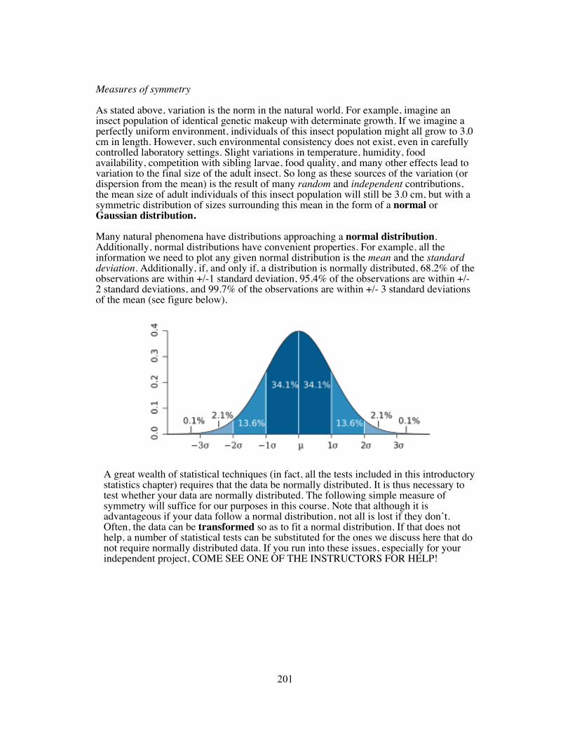
Measures of symmetry As stated above, variation is the norm in the natural world. For example, imagine an insect population of identical genetic makeup with determinate growth. If we imagine a perfectly uniform environment, individuals of this insect population might all grow to 3.0 cm in length. However, such environmental consistency does not exist, even in carefully controlled laboratory settings. Slight variations in temperature, humidity, food availability, competition with sibling larvae, food quality, and many other effects lead to variation to the final size of the adult insect. So long as these sources of the variation (or dispersion from the mean) is the result of many random and independent contributions, the mean size of adult individuals of this insect population will still be 3.0 cm, but with a symmetric distribution of sizes surrounding this mean in the form of a normal or Gaussian distribution. Many natural phenomena have distributions approaching a normal distribution. Additionally, normal distributions have convenient properties. For example, all the information we need to plot any given normal distribution is the mean and the standard deviation. Additionally, if, and only if, a distribution is normally distributed, 68.2% of the observations are within +/-1 standard deviation, 95.4% of the observations are within +/- 2 standard deviations, and 99.7% of the observations are within +/- 3 standard deviations of the mean (see figure below).

A great wealth of statistical techniques (in fact, all the tests included in this introductory statistics chapter) requires that the data be normally distributed. It is thus necessary to test whether your data are normally distributed. The following simple measure of symmetry will suffice for our purposes in this course. Note that although it is advantageous if your data follow a normal distribution, not all is lost if they don’t. Often, the data can be transformed so as to fit a normal distribution. If that does not help, a number of statistical tests can be substituted for the ones we discuss here that do not require normally distributed data. If you run into these issues, especially for your independent project, COME SEE ONE OF THE INSTRUCTORS FOR HELP!

202

We call a distribution symmetric, if the values are evenly distributed around the mean, and the mean, median and mode are identical. A distribution, in which the mean is shifted left of center of the range of values is called skewed to the left or negative skew and vice versa. (See figure below).

Pearson measure of skewness = (mean-median)/standard deviation. Values closer to 0 indicate a more symmetric distribution. The reason this simple measure works, is because the median is less susceptible to outliers than the mean. Take for instance the following example data set: 1, 1, 2, 2, 2, 2, 2, 3, 3, 3, 3, 3, 3, 4, 4, 4, 5, 5, 5, 6, 6, 7, 7, 8, 10, 15

Clearly the mode, which in this example is 3, is shifted left of the center of the range. However, both the mean and the median are influenced by the few large values of this distribution and have moved to the right of the mode, indicating that this distribution is skewed to the right. The mean (4.46 in this example) being more affected than the median, which is less influenced by outliers (3.5 in this example). The stronger the median and the mean differ from each other, the more skewed the dataset is.

203

C) Analytical Statistics We will be using four basic statistical tools for this class: X2 (chi-square tests), t-tests, analysis of variance (ANOVA), and correlation (and regressions). Chi-square tests determine whether there is a relationship between two categorical variables. t-tests are used to make comparisons of mean values of 2 groups, ANOVA is used to make comparisons of mean values of >2 groups, while correlations look for associations between two continuous variables. Details about each follow below. X2 test (chi-square test) (contingency test for independence)

A chi-square test determines whether a relationship exists between two categorical variables. (All other statistical tools we will be covering apply to dependent variables that are continuous.) Categorical data fall into distinct, mutually exclusive categories that lack quantitative intermediates: e.g. present vs. absent; female vs. male; brown vs. blue vs. green eyes. A p-value of less than 0.05 indicates that the variables are NOT independent; i.e. that two categorical variables are related. An example: We observe people to see if hair color and eye color are related. Do people with blond hair have blue eyes, etc. than expected by chance? We develop a two-way table, called a contingency table, to categorize each person into one group for each of the two categorical variables (e.g. brown hair and brown eyes, brown hair and blue eyes, brown hair and green eyes, etc.). We then study the table to see which combinations of variables have more or less observations (counts) than would be expected if there were no relationship between the two variables (hair color and eye color). To calculate this test, you must first find the expected value for the number of observations for each combination of the two variables based on the null hypothesis that the two variables are independent. Then you compare the differences in distribution of values for the expected and observed values. t-tests A t-test is, most simply, a test to determine whether there is a significant difference between two treatment means. A p-value of less than 0.05 is usually considered to indicate a significant difference between the treatment means. An example: Let’s say we want to see how the presence of a predator of dragonfly larvae alters the feeding behavior of dragonfly larvae. We could set up an experiment with 10 tanks with just a dragonfly larva, and 10 tanks with both a dragonfly larva and a predator (a total of two treatments, each with 10 replicates). We could then measure the amount

204

of dragonfly food in each tank after a specified amount of time compared to what we placed in the tank initially and use a t-test to see whether there was any difference in the mean amount of food in the 10 tanks with just dragonflies (treatment 1) and in the mean amount of food in the 10 tanks with added predators (treatment 2). ANOVA (Analysis of Variance) ANOVA looks for differences among treatments (like a t-test), by examining the variance around the mean. The main difference from a t-test is that ANOVA can look for differences in more than two means. In fact, a t-test is really just a simple type of ANOVA. What you need to know is that if the ANOVA is significant, then there is a difference among the treatments. However, if there is a significant difference, ANOVA does not tell you anything about which treatments are significantly different from the others, and you must use other tests, such as multiple pair-wise comparisons via t-tests, to determine which are significantly different from the others. So why bother doing an ANOVA first, why not just start with multiple t-tests? The reason is similar to gambling at a slot machine. Although the likelihood of winning is very small for each individual game, if you pull that slot machine often enough, eventually you will win, just by chance. Similarly, every time you do a t-test, you stand a 5% (0.05) chance of finding a difference even though there is no difference. The more t-tests you run, the greater the chance that one of your pair-wise comparisons, just by chance, shows a significant difference. This means that if you are comparing multiple means of a data set via pair-wise t-tests, the overall likelihood of finding a difference SOMEWHERE in your data set even though there is in reality no difference is greater than 0.05. The ANOVA does not have such a compounding problem. Hence, the approach is to FIRST run an ANOVA on your data set. IF the ANOVA found significant differences between means in your data set, you are now justified to look for where these differences are by doing pair-wise comparisons of the means.

An example: Let’s modify the t-test experiment that ad two treatments. Instead we have three treatments now: dragonflies alone (treatment 1), dragonflies and predator type 1 (treatment 2), and dragonflies and predator type 2 (treatment 3). We would use an ANOVA to see if there is a difference among the three treatments in the mean amount of food consumed by the dragonfly larvae.

Correlation A t-test is used to test for statistically significant differences between the means of

two different treatments. Correlations require a different kind of data. Here you have a list of subjects (individual animals, plots, ponds) and take measurements of two different continuous variables for each subject. Do subjects with a high level of

205

variable X also tend to have a high level of variable Y? These kinds of systematic associations between two variables are described by correlation.

A correlation establishes whether there is some relationship between two continuous variables – but does not determine the nature of that relationship, i.e. it cannot be translated into cause and effect. The intensity of the relationship is measured by the correlation coefficient “r”. The value of r varies between -1 and 1. -1 indicates a strong negative relationship between the two variables, 0 indicates no relationship, and 1 a strong positive relationship. If the associated p-value <0.05, we can conclude that the positive or negative relationship between the two variables is unlikely to have resulted by chance. An example: You suspect that there is some relationship between the length of a person’s thighbone and their overall height. To test this, you take a sample of people, and measure their height and the length of their thighbone for each of them. We then run a correlation using thighbone length as the X variable and height as the Y variable, or vice versa. Since in a correlation we do not assume that one variable has a direct effect on the other, but simply shows a systematic relationship in their variation, there are no dependent or independent variables for a correlation, and hence it does not matter, which variable is on which axis (BUT compare to regression!). In our example case we would probably find a relatively strong positive correlation – an r-value of above 0.8 or so, indicating that tall individuals tend to have long thigh bones and vice versa. Note however, that we did not imply that height caused long thighbones, or that long thighbones caused greater height. Nor did we determine whether thighbone length is a good predictor of height. Regression A regression is similar to a correlation. One of the key differences is that a regression DOES test whether changes in one variable are predictive of changes in the other, and provides a simple mathematical model of this relationship that can be used to predict additional values of variable Y for an untested value of variable X. For simple linear regression, this mathematical model is a straight line, following the old y = mx + b (m=slope, b=y-intercept). Once this line is established we can predict values of y from any value of x. A word of caution: It is not advisable to try to infer values of y for values of x that exceed the range of values for x that were experimentally tested in establishing the regression. The regression loses its reliability beyond the tested range. How well we can predict y from x, in other words how strong is the relationship between the two variables is measured by the coefficient of determination, or “r2” (the correlation coefficient squared). r2 ranges from 0 to 1, with 1 indicating that the values of x perfectly predict y; that is if we regress the values, all values fall exactly on the regression line (this never happens in ecology). An interesting note is that the r2 value tells us how much of the variation in our dataset is

206

explained by our statistical model (the regression line). For example, an r2 value of 0.62 indicates that our model captures 62% of the variation in the relationship of y to x. We use the p-value to assess whether the relationship observed between the two variables is due to sampling error or indicative of a real pattern. p-values < 0.05 allow you to reject the Ho that the observed relationship is due to chance – you have found a real association between the variables. An example: We have data on light intensity and algal biomass for twenty locations within a reach of stream. We suspect that higher light intensities may lead to more algal biomass. So we could run a regression on light intensity and algal biomass, using light as our x variable and algal biomass as our y variable. We end up with an equation for the regression line and an r2 value. With a high r2 value we can feel confident in using the equation for predicting values of y, based on x. An interesting note is that the r2 value tells us how much of the variation in our dataset is explained by our statistical model (the regression line). For example, an r2 value of 0.62 indicates that our model captures 62% of the variation in the relationship of y to x. NOTE: As opposed to a correlation, a regression does have dependent versus independent variables. Read the underlined sentence above again. That sentence assumes directionality in the relationship of the two variables. Light intensity is suspected to influence algal biomass, not the other way around. So light is independent, whereas algal biomass is dependent on light intensity. By convention, we plot the independent variable (light) on the x-axis, and the dependent variable (algal biomass) on the y-axis. Another way of thinking about this is that the independent variable is the variable manipulated by us during the experiment (light) to test the response in the dependent variable (algal biomass). We are not likely to try to manipulate algal biomass and expect the light intensity striking the water surface to change as a result. Which variable is the independent vs. dependent, and hence whether it is plotted on the x or the y-axis DOES make a difference in a regression. The reason is that a regression determines the deviations of each data point from the best-fit line (the regression line). There are two directions in which these deviations can be measured: in a horizontal direction, and a vertical direction (see figures below). When we ask: how well can X predict Y, we are interested only in the deviations from the line in the vertical, y-direction. If we confuse which variable is the dependent vs. independent, we calculate a best-fit line in the horizontal, or X-direction, and receive a different (and wrong) answer.

207

SUMMARY: How to choose among statistical tests Chi-square done on count data collected for two categorical variables, to address a question in the form of “Do distributions differ?” e.g.: Is the distribution of eye color independent from the distribution of hair color? t-test done on discrete or continuous data collected for one categorical variable with only two treatments to address a question in the form of “Do means of the two treatments differ?” e.g. Does presence of a predator affect the amount of food consumed by a dragonfly larva? ANOVA done on discrete or continuous data collected for one categorical variable with more than two treatments, to address a question in the form of “Do means of >2 treatments differ?” e.g. Does the predator type affect the amount of food consumed by a dragonfly larva? Correlation done on two continuous variables; no independent-dependent variables; to address a question in the form of “is there a relationship between these variables?”. Regression done on two continuous variables; clear independent-dependent variable distinction, to address a question in the form of “how well can we predict the dependent variable based on the independent variable?” A regression with a high coefficient of determination may hint at a causal relationship, but causality has to be tested by a manipulative experiment subsequently.

208

209

III) Calculating your statistics (*Note: these instructions are written for Microsoft Office 2003/2004 (PC/Mac) versions, not the 2007/2008 Office.) Here you will find instructions on how to calculate and plot each of the statistical procedures described in Section II) in the sequence they were introduced. A) HISTOGRAMS Construction of histograms by hand 3. First decide on the best bin width (and hence the number of bins needed to cover the

data range) based on maximum and minimum population values and the sample size. If most bins don't have at least several values that fall within them, then the bin size should be increased. Try something like sample size divided by # of bins equals or is larger than 5-10. Another rule of thumb is to choose your number of bins as the square root of n, (n = sample size). Your bins should be the same width.

4. Decide on what value to start your bin boundaries with. As you will see it can make a difference, especially for sample sets with a smaller n.

5. Count the number of population values that fall within a certain bin. If the value is equal to the bin boundary, typically it counts in the bin to the right (a greater than or equal to rule).

6. Plot the bin boundaries along the x-axis. Plot columns in the y direction whose height is equal to the number of values from the population within a given bin. Alternatively, you may also plot columns as the %-value of the counts within a bin with respect to the total sample size.

Construction of histograms in Excel The initial steps are the same as described above. There are two ways to obtain a histogram in Excel: Using the FREQUENCY function: 1. I suggest you avoid this until you become or are more familiar with Excel. How

it operates differs from one Excel version to another. In some situations it can provide some greater flexibility.

2. Insert sample data in a column. If you have a lot of data you may want to sort it first to find the minimum and maximum numbers.

3. Create an array of bin values in descending order. 4. Use the FREQUENCY function, selecting the data and bin arrays when asked. 5. The frequency function should return an array of numbers that are the values in

each bin. You may have to drag/copy the first cell downwards to create the array.

6. Idiosyncrasies of the Excel FREQUENCY function. If you have your bin values in ascending order it computes a cumulative frequency. If you have your bin values in descending order it computes a standard frequency. Bottom line, always - check out your numbers to make sure they make sense. For older versions of Excel you can try using control-shift-enter for the FREQUENCY function. One Excel source indicates that this should yield an array instead of a single number. In some versions of Excel on some platforms you may want to fix your data cell reference with a $.

7. Use the column plot to look at the results. You can plot multiple histograms at once. If you look in the Series window there is a place to label the bin intervals by choosing your bin array. Check your x axis labeling to make sure you are plotting bin intervals. Unfortunately Excel is not very good about placement of x labels.

210

8. Using the histogram routine (the suggested route): 9. The Histogram routine is found under Tools, under Data Analysis. This is an

add-in and if you can't find it you may need to install it. Look under Tools at the Add-ins option. If you are lucky you won't need the CD. It varies from platform to platform and by Excel version.

10. Choose the Histogram insert the data and bin arrays in the appropriate spot in the input box. Choose what type of output you want. Make sure you select the chart option. Notice that this will put the results into a separate sheet. Select finish and, that's it, your done.

Population distributions vs. histograms: with increasing n (n = sample size) and smaller and more bins the histogram should approach a curve, i.e. a continuous frequency distribution.

B) DESCRIPTIVE STATISTICS The formulae and definitions for calculating the various descriptive statistics are given with their explanation in Section II) of this booklet. Excel univariate statistical functions: Below is a list of functions you may find useful in describing distribution characteristics. You can find a list of Excel functions under Insert > Function. You should familiarize yourself with the array of functions available to you. If you want to enter a formula into a cell, start with the equal sign. Then you can build the equation afterwards using standard mathematical operators and by inserting function commands.

Available functions include: AVERAGE, FREQUENCY, MEDIAN, MODE, RANK, SKEW, SORT, STDEV (for standard deviation), VAR (for variance).

The function arguments (the numbers it acts on) are placed within parentheses after the function. For statistical functions an array of numbers is input into the function, usually using cell references for the beginning and end of the array. For example typing"=AVERAGE(A1:A36)" in a cell will calculate the average of the numbers in the array of cells from A1 through A36.

Note that Excel describes what the function does when you insert it into the formula bar. Help will also give you a more complete description. The frequency function can be a bit tricky to use.

211

C) T-TEST Requires: 1 categorical independent variable with 2 treatments and 1 dependent variable

a) Use Excel to make a figure 1. Calculate the average and the SE (standard error) for each treatment.

(Think about why you need to use the standard error, and not the standard deviation!). Create the following type of table in the Excel spreadsheet:

Treatment Average SE Category 1 [Fill in your calculated values] … Category 2 … …

2. Highlight the 6 cells in the first 2 columns of the table. MAC: Click on chart wizard (with bar chart) icon that is located in the toolbar. PC: From the menu bar, pull down Insert and click ‘Chart’. Click on the type of chart and subtype you want to make. Click ‘next’. (We recommend using a bar graph in this instance).

3. Do NOT give the Figure a title. Label x-axis (horizontal with independent variable); label y-axis (vertical with dependent variable).

4. Clean up your graph while on the sheet for labeling axes. (Remove extra legends, gridlines, background coloration, etc). (Click on gridlines in menu and un-do check next to gridline box, etc)

i) Select ‘next’; select ‘as object in sheet 1’; select ‘finish’.

ii) To change the x-axis so that it starts at 0, click on the axis. Select scale. Minimum = 0.

5. Add Standard Error bars to each average. i) MAC: double click inside one bar; select ‘Y error

bars’. PC: right click inside a bar; select Format Data Series select ‘Y error bars’.

For both MAC and PC: ii) For display, select ‘both’. For Error Amount, select

‘Custom’. Select triangle (or icon) to R. iii) Highlight SE data from worksheet (for +bar).

Repeat for –bar. 6. In a cell BELOW the figure, create a figure caption (we also call this a

figure legend). The rule of thumb is that the reader should completely understand the figure without reading any of the text of the paper. Include what the bar and vertical lines indicate (mean +/- SE). Keep it to one complete ‘sentence’. For example:

“Figure 1. Comparison of plant species richness (mean +/- SE) between two fields abandoned for one vs. five years.”

212

b) Use Excel to do a t-test 1. Method 1. Observe the SE bars of the Figure. If the top of one

bar and the bottom of the second bar do NOT overlap, then the difference between the means of the two years is likely to be statistically significant. (Do this first to get an estimate of significance. Then do Method 2).

2. Method 2. A statistical test 1. Click a cell on the worksheet. Select ‘fx’ in the toolbar.

Select ‘Statistical’, then TTEST. OK. 2. Array 1 = original data from treatment 1.

Array 2 = original data from treatment 2. Tails = 2 (2-tailed t-test). Type = 3 (2-sample test with unequal variance). OK.

3. The probability value is printed on the worksheet. If it is P < 0.05, then there is less than a 5% probability that the difference between the two means is due to chance

c) Interpretation of results

a. Return to your ‘Hypothesis/Prediction’. b. Based on your analysis, what can you conclude? Do the data support your

hypothesis? c. To write up the “Results” section of a scientific manuscript, summarize

the main pattern in your figure, state the statistical output, and refer to Figure 1 (in parentheses at the end of sentence). Keep the results of a t-test to 1 sentence. For example:

“The mean plant species richness is significantly (or non-significantly, depending on what your result is) greater in the X-year than the X-year field (t-test P < 0.05) (Fig. 1).”

213

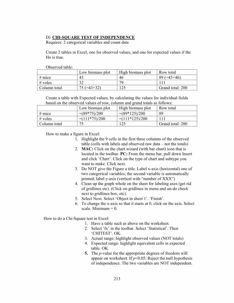
D) CHI-SQUARE TEST OF INDEPENDENCE Requires: 2 categorical variables and count data Create 2 tables in Excel, one for observed values, and one for expected values if the Ho is true. Observed table:

Low biomass plot High biomass plot Row total # mice 43 46 89 (=43+46) # voles 32 79 111 Column total 75 (=43+32) 125 Grand total: 200

Create a table with Expected values, by calculating the values for individual fields based on the observed values of row, column and grand totals as follows:

Low biomass plot High biomass plot Row total # mice =(89*75)/200 =(89*125)/200 89 # voles =(111*75)/200 =(111*125)/200 111 Column total 75 125 Grand total: 200

How to make a figure in Excel:

1. Highlight the 9 cells in the first three columns of the observed table (cells with labels and observed raw data – not the totals)

2. MAC: Click on the chart wizard (with bar chart) icon that is located in the toolbar. PC: From the menu bar, pull down Insert and click ‘Chart’. Click on the type of chart and subtype you want to make. Click next.

3. Do NOT give the Figure a title. Label x-axis (horizontal) one of two categorical variables; the second variable is automatically printed; label y-axis (vertical with “number of XXX”)

4. Clean up the graph whole on the sheet for labeling axes (get rid of gridlines etc). (Click on gridlines in menu and un-do check next to gridlines box, etc).

5. Select Next. Select ‘Object in sheet 1’. ‘Finish’. 6. To change the x-axis so that it starts at 0, click on the axis. Select

scale. Minimum = 0. How to do a Chi-Square test in Excel:

1. Have a table such as above on the worksheet. 2. Select ‘fx’ in the toolbar. Select ‘Statistical’. Then

‘CHITEST’. OK. 3. Actual range: highlight observed values (NOT totals) 4. Expected range: highlight equivalent cells in expected

table. OK. 5. The p-value for the appropriate degrees of freedom will

appear on worksheet. If p<0.05: Reject the null hypothesis of independence. The two variables are NOT independent.

214

E) CORRELATION / REGRESSION Requires: two continuous variables. How to create figure in Excel:

1. Have the data for the 2 variables in the first two columns of the worksheet. 2. Make a (XY) scattergram (scatterplot) figure

i. Select chart wizard in tool bar ii. Chart type: XY (Scatter); chart subtype: upper left

iii. Data range: select all cells on worksheet with data. iv. Don’t give a title to your figure. Label the x (include units) and

y-axes. v. Save as object in Sheet 1. Move to lower left of page.

vi. In a cell BELOW the figure, create a figure caption (we also call this a figure legend). The rule of thumb is that the reader should completely understand the figure without reading any of the text of the paper. Keep it to one complete ‘sentence’. For example:

“Figure 1. Number of fruits as a function of total leaf area (cm2) of a pawpaw tree.”

How to calculate CORRELATION statistic in Excel: (no cause-effect in x and y)

1. Calculate the correlation coefficient = r, which measures the strength of association between the two variables.

a. Type ‘correlation’ in a cell below column A data. Select cell to its right.

b. Select fx in the toolbar, then ‘statistical’, then ‘correl’. c. Array1: Select data in column A d. Array 2: Select data in column B. OK.

Interpretation of results:

1. Whether r = significant depends on the degrees of freedom. The critical value that r must be greater than to be significant (P<0.05) will have to be looked up in a correlation table (found at the end of this section). A p-value <0.05 indicates that the relationship (either positive or negative) that you observe between the two variables is due to chance. There is a systematic relationship.

2. Based on your data what can you conclude? Do the data support your hypothesis?

3. To write up the “Results” section of a manuscript, summarize the main pattern in your figure. State the statistical output and refer to Fig. 1 in parentheses at the end of the sentence. Keep the results of a correlation to 1 sentence. Example:

“Number of fruits did not increase significantly as total leaf area of the tree increased (r = 0.523, P > 0.05) (Fig.1).”

215

How to calculate REGRESSION statistic in Excel: (assuming cause-effect in x and y) THE QUICK AND DIRTY WAY:

1. Add a regression line to the above figure. a. MAC: highlight chart area within figure. From chart menu select “Add

trendline”, for type tab, select “linear” b. PC: right click on one point in the figure. Do as above for MAC.

2. Calculate r2 (values range from 0 to 1) a. Highlight chart area within figure b. From chart menu select add trendline c. For type tab select ‘options’ d. Check ‘display r2 value on chart’ e. Interpret the r2 value. How well does the line represent the data points?

3. Get an equation for the regression line. a. Highlight chart area b. From chart menu, select ‘Add Trendline’ c. For Type tab, select ‘options’ d. Check ‘Display equation on chart’ e. This equation allows you to predict further y values for any given x

value.

THE THOROUGH WAY: (the only way to get a p-value for your regression) 1. Select ‘TOOLS’, then ‘DATA ANALYSIS’. (If you don’t see it, select

“Add-Ins” and then select “Analysis Tool Pac” to install the data analysis tools; this has to be done only once. Go back and select “Data Analysis” from the Tools menu.)

2. Select ‘REGRESSION’. 3. Input the dependent variable in the field “INPUT Y RANGE” by

highlighting the appropriate values in the spreadsheet. Input the independent variable in the field “INPUT X RANGE” similarly.

4. Under “OUTPUT OPTIONS” select “NEW WORKSHEET PLY”. OK. 5. Interpretation of output: you get an r2 value, as well as two p-values. The

r2 value indicates what proportion of the variation is explained by your model (the linear regression line). The p-value you are interested in to test whether the relationship between your variables is due to sampling error is the p-value associated with the x-variable. (Ignore the p-value of the y-intercept for the purposes of this course). A p-value of <0.05 indicates that the relationship you are testing is unlikely to be due to sampling error.

F) ANOVA Requires: 1 categorical independent variable with > 2 treatments. How to create a figure in Excel:

Follow directions under t-test. How to do an ANOVA test in Excel:

1. Data must be organized with each treatment in a separate column.

216

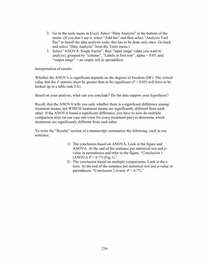
2. Go to the tools menu in Excel. Select “Data Analysis” at the bottom of the menu. (If you don’t see it, select “Add-Ins” and then select “Analysis Tool Pac” to install the data analysis tools; this has to be done only once. Go back and select “Data Analysis” from the Tools menu.)

3. Select “ANOVA: Single Factor”, then “input range” (data you want to analyze), grouped by “column”, “Labels in first row”, alpha = 0.05, and “output range” = an empty cell in spreadsheet.

Interpretation of results: Whether the ANOVA is significant depends on the degrees of freedom (DF). The critical value that the F-statistic must be greater than to be significant (P < 0.05) will have to be looked up in a table (ask TA). Based on your analysis, what can you conclude? Do the data support your hypothesis? Recall, that the ANOVA tells you only whether there is a significant difference among treatment means, not WHICH treatment means are significantly different from each other. If the ANOVA found a significant difference, you have to now do multiple comparison tests (in our case one t-test for every treatment pair) to determine which treatments are significantly different from each other. To write the “Results” section of a manuscript, summarize the following, each in one sentence:

1) The conclusion based on ANOVA. Look at the figure and ANOVA. At the end of the sentence put statistical test and p- value in parentheses and refer to the figure. “Conclusion 1 (ANOVA P < 0.??) (Fig.1).”

2) The conclusion based on multiple comparisons. Look at the t-tests. At the end of the sentence put statistical test and p-value in parentheses. “Conclusion 2 (t-test, P < 0.??).”

217

CHI-SQUARE STATISTICAL TABLE (Critical Values) DF !=0.10 !=0.05 !=0.025 !=0.01 DF !=0.10 !=0.05 !=0.02 !=0.01 1 2.706 3.841 5.024 6.635 21 29.615 32.671 35.479 38.932 2 4.605 5.991 7.378 9.210 22 30.813 33.924 36.781 40.289 3 6.251 7.815 9.348 11.345 23 32.007 35.172 38.076 41.638 4 7.779 9.488 11.143 13.277 24 33.196 36.415 39.364 42.980 5 9.236 11.070 12.833 15.086 25 34.382 37.652 40.646 44.314 6 10.645 12.592 14.449 16.812 26 35.563 38.885 41.923 45.642 7 12.017 14.067 16.013 18.475 27 36.741 40.113 43.195 46.963 8 13.362 15.507 17.535 20.090 28 37.916 41.337 44.461 48.278 9 14.684 16.919 19.023 21.666 29 39.088 42.557 45.772 49.588 10 15.987 18.307 20.483 23.209 30 40.256 43.773 46.979 50.892

11 17.275 19.675 21.920 24.725 31 41.422 44.985 48.232 52.191 12 18.549 21.026 23.337 26.217 32 42.585 46.194 49.480 53.486 13 19.812 22.362 24.736 27.688 33 43.745 47.400 50.725 54.776 14 21.064 23.685 26.119 29.141 34 44.903 48.602 51.966 56.061 15 22.307 24.996 27.488 30.578 35 46.059 49.802 53.203 57.302

16 23.542 26.296 28.845 32.000 36 47.212 50.998 54.437 58.619 17 24.769 27.587 30.191 33.409 37 48.363 52.192 55.668 59.893 18 25.989 28.869 31.526 34.805 38 49.513 53.384 56.896 61.162 19 27.204 30.144 32.852 36.191 39 50.660 54.572 58.120 62.428 20 28.412 31.410 34.170 37.566 40 51.805 55.758 59.342 63.691

1) Calculate DF (degrees of freedom) = (row-1) (column-1). 2) Locate this DF in the table. 3) Use this row of threshold values. 4) Read across this row from left to right until you find a value greater than your

calculated chi-square statistic. 5) The p-value for your observation is the p-value at the top of the first column to the

left of your value. e.g. if your chi-square statistic for DF=1 is 4.201, then P < 0.05; if your statistic is

7.735, then P < 0.01. A P < 0.05 (or smaller) value indicates that you can reject the null hypothesis that the

variables are independent. In other words, you have evidence the variables are significantly related.

If your chi-square statistic value lies to the left of the ! = 0.05 column, then your results are not significant (n.s. P > 0.05). You cannot reject the null hypothesis that the variables are independent. You cannot conclude that the variables are dependent (related).

218

PEARSON’S CORRELATION COEFFICIENT r (Critical Values)

Level of Significance for a One-Tailed Test .05 .025 .01 .005 .0005 .05 .025 .01 .005 .0005

Level of Significance for a Two-Tailed Test df=(N-2) .10 .05 .02 .01 .001 df=(N-2) .10 .05 .02 .01 .001

1 0.988 0.997 0.9995 0.9999 0.99999 21 0.352 0.413 0.482 0.526 0.640 2 0.900 0.950 0.980 0.990 0.999 22 0.344 0.404 0.472 0.515 0.629 3 0.805 0.878 0.934 0.959 0.991 23 0.337 0.396 0.462 0.505 0.618 4 0.729 0.811 0.882 0.971 0.974 24 0.330 0.388 0.453 0.496 0.607 5 0.669 0.755 0.833 0.875 0.951 25 0.323 0.381 0.445 0.487 0.597

6 0.621 0.707 0.789 0.834 0.928 26 0.317 0.374 0.437 0.479 0.588 7 0.582 0.666 0.750 0.798 0.898 27 0.311 0.367 0.430 0.471 0.579 8 0.549 0.632 0.715 0.765 0.872 28 0.306 0.361 0.423 0.463 0.570 9 0.521 0.602 0.685 0.735 0.847 29 0.301 0.355 0.416 0.456 0.562

10 0.497 0.576 0.658 0.708 0.823 30 0.296 0.349 0.409 0.449 0.554

11 0.476 0.553 0.634 0.684 0.801 40 0.257 0.304 0.358 0.393 0.490 12 0.457 0.532 0.612 0.661 0.780 60 0.211 0.250 0.295 0.325 0.408 13 0.441 0.514 0.592 0.641 0.760 120 0.150 0.178 0.210 0.232 0.294 14 0.426 0.497 0.574 0.623 0.742 ! 0.073 0.087 0.103 0.114 0.146 15 0.412 0.482 0.558 0.606 0.725

16 0.400 0.468 0.542 0.590 0.708 17 0.389 0.456 0.529 0.575 0.693 18 0.378 0.444 0.515 0.561 0.679 19 0.369 0.433 0.503 0.549 0.665 20 0.360 0.423 0.492 0.537 0.652

6) Decide if you should use a One-Tailed or Two-Tailed Test:

a. One-Tail: if you have an a priori hypothesis as to the sign (- or +) of the correlation. b. Two-Tail: if you have no a prior hypothesis as to the sign of the correlation.

7) Calculate df (degrees of freedom) = N (sample size) -2). 8) Locate this df in the table. 9) Use this row of threshold values. 10) Read across this row from left to right until you find a value greater than your

calculated r statistic. 11) The p–value for your observation is the p–value at the top of the first column to the

left of your value. e.g. if r for df = 15 is 0.523, then P < 0.025 for a One-Tailed Test; if r is 0.599, then P < 0.01.

7) A P < 0.05 (or smaller) value indicates that you can reject the null hypothesis that the two variables are not correlated. In other words, you have evidence the variables are significantly related. If your r statistic value lies to the left of the 0.05 column, then your results are not significant (n.s. P > 0.05). You cannot reject the null hypothesis that the variables are unrelated.