9-1 hypothesis testing - ucla statistics
TRANSCRIPT

4-6 Normal Distribution
5-5 Linear Combinations of Random Variables
1-1 The Engineering Method and
Statistical Thinking
Figure 1.1 The engineering method

The field of statistics deals with the collection,
presentation, analysis, and use of data to
•! Make decisions
•! Solve problems
•! Design products and processes
1-1 The Engineering Method and
Statistical Thinking
•! Statistical techniques are useful for describing and
understanding variability.
•! By variability, we mean successive observations of a
system or phenomenon do not produce exactly the same
result.
•! Statistics gives us a framework for describing this
variability and for learning about potential sources of
variability.
1-1 The Engineering Method and
Statistical Thinking

Engineering Example
An engineer is designing a nylon connector to be used in an
automotive engine application. The engineer is considering
establishing the design specification on wall thickness at 3/32
inch but is somewhat uncertain about the effect of this decision
on the connector pull-off force. If the pull-off force is too low, the
connector may fail when it is installed in an engine. Eight
prototype units are produced and their pull-off forces measured
(in pounds): 12.6, 12.9, 13.4, 12.3, 13.6, 13.5, 12.6, 13.1.
1-1 The Engineering Method and
Statistical Thinking
Engineering Example
•!The dot diagram is a very useful plot for displaying a small
body of data - say up to about 20 observations.
•! This plot allows us to see easily two features of the data; the
location, or the middle, and the scatter or variability.
1-1 The Engineering Method and
Statistical Thinking

Engineering Example
•! The engineer considers an alternate design and eight prototypes
are built and pull-off force measured.
•! The dot diagram can be used to compare two sets of data
Figure 1-3 Dot diagram of pull-off force for two
wall thicknesses.
1-1 The Engineering Method and
Statistical Thinking
Engineering Example
•! Since pull-off force varies or exhibits variability, it is a
random variable.
•! A random variable, X, can be model by
X = µ + !
where µ is a constant and ! a random disturbance.
1-1 The Engineering Method and
Statistical Thinking
1-1 The Engineering Method and
Statistical Thinking
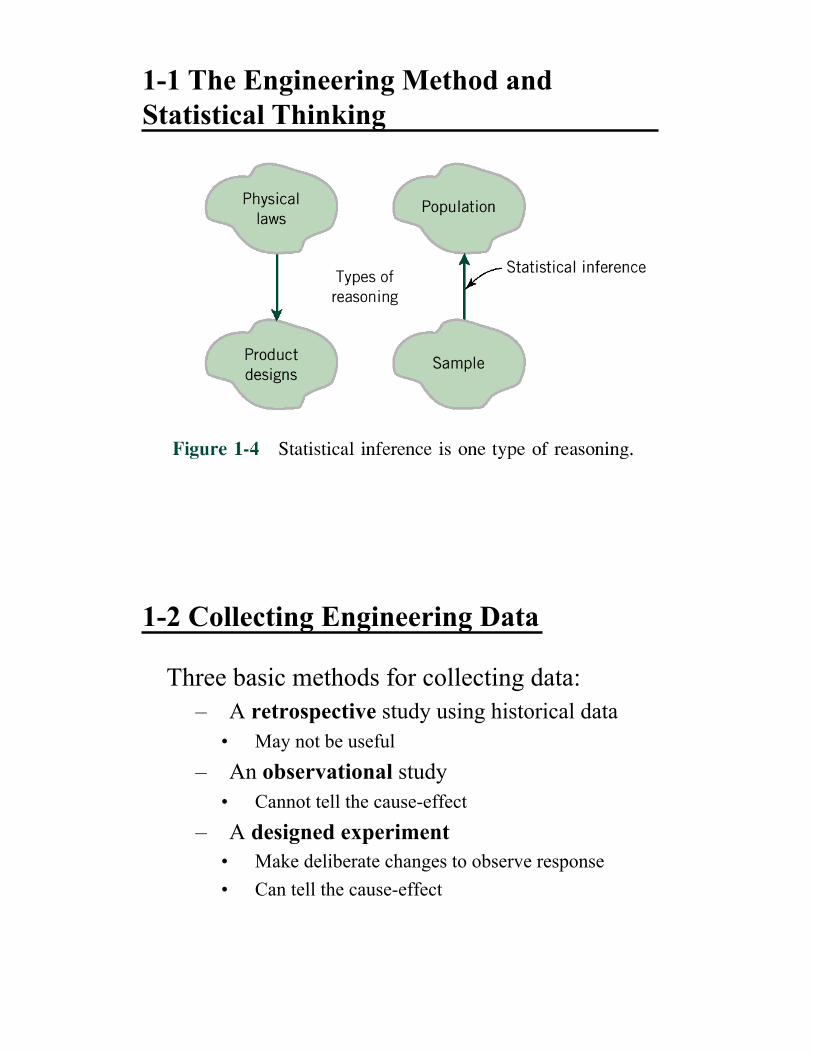
Three basic methods for collecting data:
–! A retrospective study using historical data
•! May not be useful
–! An observational study
•! Cannot tell the cause-effect
–! A designed experiment
•! Make deliberate changes to observe response
•! Can tell the cause-effect
1-2 Collecting Engineering Data
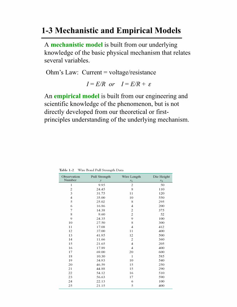
1-3 Mechanistic and Empirical Models
A mechanistic model is built from our underlying
knowledge of the basic physical mechanism that relates
several variables.
Ohm’s Law: Current = voltage/resistance
I = E/R or I = E/R + !
An empirical model is built from our engineering and
scientific knowledge of the phenomenon, but is not
directly developed from our theoretical or first-
principles understanding of the underlying mechanism.

Figure 1-15 Three-dimensional plot of the wire and pull
strength data.
1-3 Mechanistic and Empirical Models
In general, this type of empirical model is called a
regression model.
The estimated regression line is given by

Figure 1-16 Plot of the predicted values of pull strength
from the empirical model.
4-6 Normal Distribution
Definition

4-6 Normal Distribution
Figure 4-10 Normal probability density functions
for selected values of the parameters µ and "2.
4-6 Normal Distribution
Definition : Standard Normal

4-6 Normal Distribution
Example 4-11
Figure 4-13 Standard normal probability density
function.
4-6 Normal Distribution
Standardizing

4-6 Normal Distribution
Example 4-13
4-6 Normal Distribution
Figure 4-15 Standardizing a normal random
variable.

4-6 Normal Distribution
To Calculate Probability
4-6 Normal Distribution
Example 4-14 (continued)

4-6 Normal Distribution
Example 4-14 (continued)
Figure 4-16 Determining the value of x to meet a
specified probability.
5-5 Linear Combinations of Random
Variables
Definition
Mean of a Linear Combination

5-5 Linear Combinations of Random
Variables
Variance of a Linear Combination
5-5 Linear Combinations of Random
Variables
Example 5-33

5-5 Linear Combinations of Random
Variables
Mean and Variance of an Average
5-5 Linear Combinations of Random
Variables
Reproductive Property of the Normal Distribution

5-5 Linear Combinations of Random
Variables
Example 5-34
Some useful results to remember
For any normal random variable
– 3 x! ! – 2µ ! – ! ! ! +! ! + 2! ! + 3! !
68%
95%
99.7%
f (x)
MONTGOMERY: Applied Statistics, 3eFig. 4.12 W-68

6-1 Numerical Summaries
Definition: Sample Mean
Definition: Sample Range
6-1 Numerical Summaries
Example 6-1
6-1 Numerical Summaries
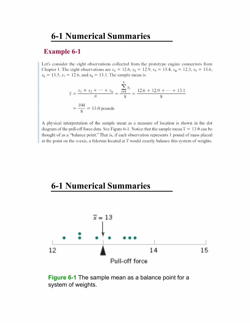
Figure 6-1 The sample mean as a balance point for a
system of weights.

6-1 Numerical Summaries
Population Mean
For a finite population with N (equally likely)
measurements, the mean is
The sample mean is a reasonable estimate of the
population mean.
6-1 Numerical Summaries
Definition: Sample Variance
•! n-1 is referred to as the degrees of freedom.

6-1 Numerical Summaries
How Does the Sample Variance Measure Variability?
Figure 6-2 How the sample variance measures variability
through the deviations . xxi!
6-1 Numerical Summaries
Example 6-2
6-1 Numerical Summaries
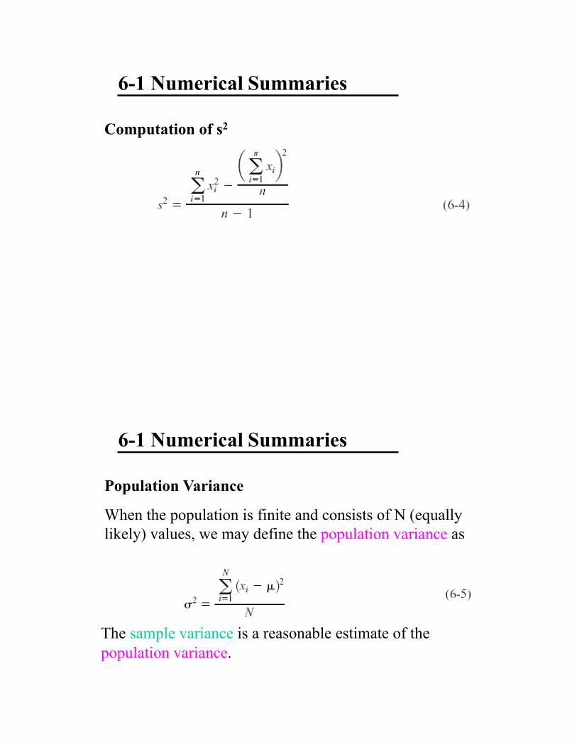
Computation of s2
6-1 Numerical Summaries
Population Variance
When the population is finite and consists of N (equally
likely) values, we may define the population variance as
The sample variance is a reasonable estimate of the
population variance.
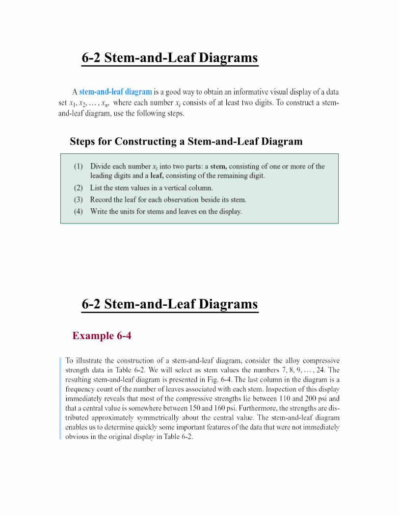
6-2 Stem-and-Leaf Diagrams
Steps for Constructing a Stem-and-Leaf Diagram
6-2 Stem-and-Leaf Diagrams
Example 6-4

6-2 Stem-and-Leaf Diagrams
6-2 Stem-and-Leaf Diagrams
Figure 6-4 Stem-and-
leaf diagram for the
compressive strength data in Table 6-2.
6-2 Stem-and-Leaf Diagrams
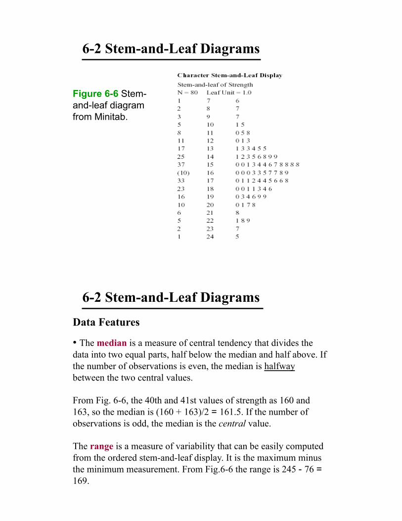
Figure 6-6 Stem-
and-leaf diagram
from Minitab.
Data Features
•! The median is a measure of central tendency that divides the
data into two equal parts, half below the median and half above. If
the number of observations is even, the median is halfway
between the two central values.
From Fig. 6-6, the 40th and 41st values of strength as 160 and
163, so the median is (160 + 163)/2 = 161.5. If the number of
observations is odd, the median is the central value.
The range is a measure of variability that can be easily computed
from the ordered stem-and-leaf display. It is the maximum minus
the minimum measurement. From Fig.6-6 the range is 245 - 76 =
169.
6-2 Stem-and-Leaf Diagrams

Data Features
•!When an ordered set of data is divided into four equal parts, the
division points are called quartiles.
•!The first or lower quartile, q1 , is a value that has approximately
one-fourth (25%) of the observations below it and approximately
75% of the observations above.
•!The second quartile, q2, has approximately one-half (50%) of
the observations below its value. The second quartile is exactly
equal to the median.
•!The third or upper quartile, q3, has approximately three-fourths
(75%) of the observations below its value. As in the case of the
median, the quartiles may not be unique.
6-2 Stem-and-Leaf Diagrams
Data Features
•! The compressive strength data in Figure 6-6 contains
n = 80 observations. Minitab software calculates the first and third
quartiles as the(n + 1)/4 and 3(n + 1)/4 ordered observations and
interpolates as needed.
For example, (80 + 1)/4 = 20.25 and 3(80 + 1)/4 = 60.75.
Therefore, Minitab interpolates between the 20th and 21st ordered
observation to obtain q1 = 143.50 and between the 60th and
61st observation to obtain q3 =181.00.
6-2 Stem-and-Leaf Diagrams

Data Features
•! The interquartile range is the difference between the upper
and lower quartiles, and it is sometimes used as a measure of
variability.
•! In general, the 100kth percentile is a data value such that
approximately 100k% of the observations are at or below this
value and approximately 100(1 - k)% of them are above it.
6-2 Stem-and-Leaf Diagrams
6-4 Box Plots
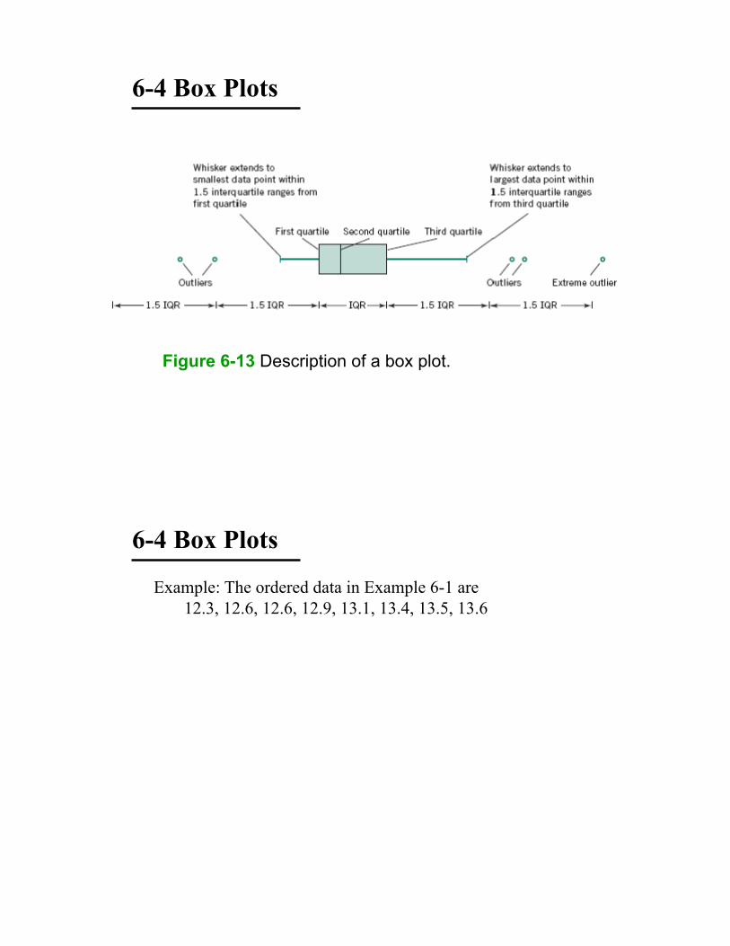
•! The box plot is a graphical display that
simultaneously describes several important features of
a data set, such as center, spread, departure from
symmetry, and identification of observations that lie
unusually far from the bulk of the data.
•! Whisker
•! Outlier
•! Extreme outlier
6-4 Box Plots
Figure 6-13 Description of a box plot.
6-4 Box Plots
Example: The ordered data in Example 6-1 are
12.3, 12.6, 12.6, 12.9, 13.1, 13.4, 13.5, 13.6
6-4 Box Plots
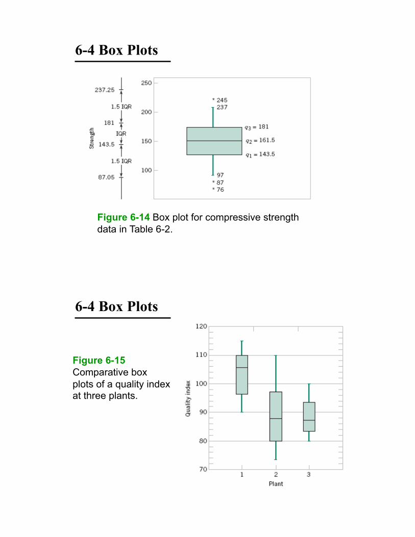
Figure 6-14 Box plot for compressive strength
data in Table 6-2.
6-4 Box Plots
Figure 6-15
Comparative box
plots of a quality index at three plants.
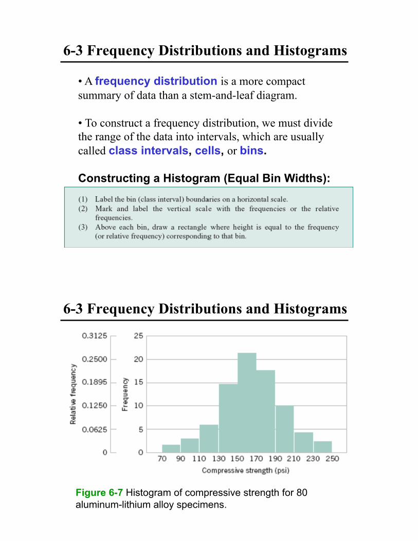
6-3 Frequency Distributions and Histograms
•! A frequency distribution is a more compact
summary of data than a stem-and-leaf diagram.
•! To construct a frequency distribution, we must divide
the range of the data into intervals, which are usually
called class intervals, cells, or bins.
Constructing a Histogram (Equal Bin Widths):
6-3 Frequency Distributions and Histograms
Figure 6-7 Histogram of compressive strength for 80
aluminum-lithium alloy specimens.

6-3 Frequency Distributions and Histograms
Figure 6-8 A histogram of the compressive strength data
from Minitab with 17 bins.
6-3 Frequency Distributions and Histograms
Figure 6-11 Histograms for symmetric and skewed distributions.

6-6 Probability Plots
•! Probability plotting is a graphical method for
determining whether sample data conform to a
hypothesized distribution based on a subjective visual
examination of the data.
•! Probability plotting typically uses special graph
paper, known as probability paper, that has been
designed for the hypothesized distribution. Probability
paper is widely available for the normal, lognormal,
Weibull, and various chi-square and gamma
distributions.
6-6 Probability Plots
Example 6-7

6-6 Probability Plots
Example 6-7 (continued)
6-6 Probability Plots
Figure 6-19 Normal
probability plot for
battery life.

6-6 Probability Plots
Figure 6-20 Normal
probability plot
obtained from standardized normal
scores.
6-6 Probability Plots
Figure 6-21 Normal probability plots indicating a nonnormal
distribution. (a) Light-tailed distribution. (b) Heavy-tailed
distribution. (c ) A distribution with positive (or right) skew.

6-5 Time Sequence Plots
•! A time series or time sequence is a data set in
which the observations are recorded in the order in
which they occur.
•! A time series plot is a graph in which the vertical
axis denotes the observed value of the variable (say x)
and the horizontal axis denotes the time (which could
be minutes, days, years, etc.).
•! When measurements are plotted as a time series, we
often see
•!trends,
•!cycles, or
•!other broad features of the data
6-5 Time Sequence Plots
Figure 6-16 Company sales by year (a) and by quarter (b).

6-5 Time Sequence Plots
Figure 6-18 A digidot plot of chemical process concentration
readings, observed hourly.
Some Useful Comments
•! Locations: mean and median
•! Spreads: standard deviation (s.d.) and IQR
–! Mean and s.d. are sensitive to extreme values (outliers)
–! Median and IQR are resistant to extreme values and
are better for skewed distributions
–! Use mean and s.d. for symmetrical distributions without
outliers
•! Software has defaults, which may not be the best
choice
–! How many stems or bins?
–! The reference line in a normal probability plot.
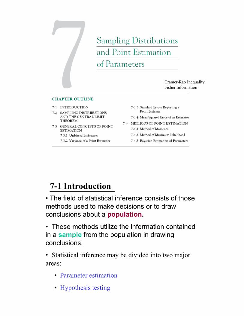
Cramer-Rao Inequality
Fisher Information
7-1 Introduction
•! The field of statistical inference consists of those
methods used to make decisions or to draw
conclusions about a population.
•! These methods utilize the information contained
in a sample from the population in drawing
conclusions.
•! Statistical inference may be divided into two major
areas:
•! Parameter estimation
•! Hypothesis testing

Definition
7-1 Introduction
7-1 Introduction

7-1 Introduction
7.2 Sampling Distributions and the
Central Limit Theorem
Statistical inference is concerned with making decisions about a
population based on the information contained in a random
sample from that population.
Definitions:

7.2 Sampling Distributions
Figure 6-3
Relationship between a
population and a sample.
Suppose X1, …, Xn are a random sample from a population
with mean µ and variance !2.
(a) What are the mean and variance of the sample mean?
(b) What is the sampling distribution of the sample mean if
the population is normal.
7.2 Sampling Distributions
7.2 Sampling Distributions and the
Central Limit Theorem
If the population is normal, the sampling distribution of Z is exactly standard normal.
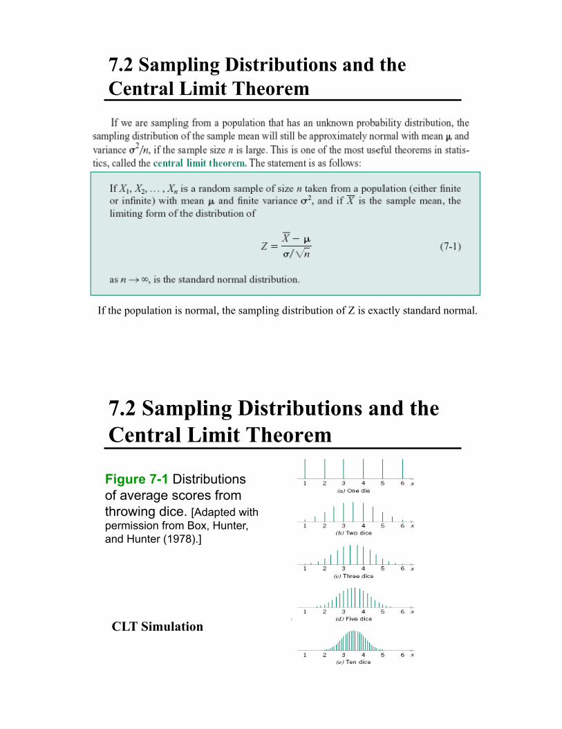
7.2 Sampling Distributions and the
Central Limit Theorem
Figure 7-1 Distributions
of average scores from
throwing dice. [Adapted with
permission from Box, Hunter,
and Hunter (1978).]
CLT Simulation
7.2 Sampling Distributions and the
Central Limit Theorem
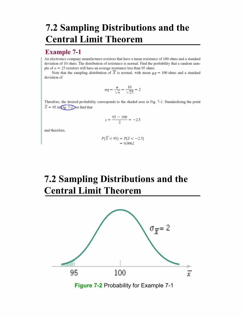
Example 7-1
7.2 Sampling Distributions and the
Central Limit Theorem
Figure 7-2 Probability for Example 7-1
7.2 Sampling Distributions and the
Central Limit Theorem
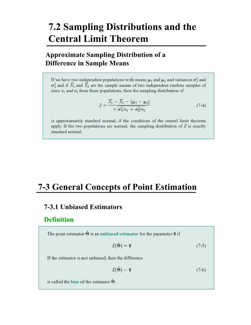
Approximate Sampling Distribution of a
Difference in Sample Means
7-3 General Concepts of Point Estimation
7-3.1 Unbiased Estimators
Definition
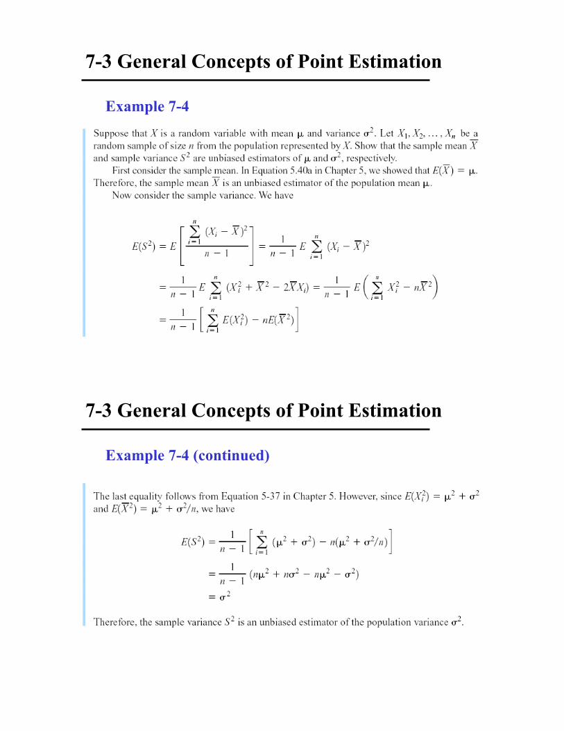
Example 7-4
7-3 General Concepts of Point Estimation
Example 7-4 (continued)
7-3 General Concepts of Point Estimation

7-3.2 Variance of a Point Estimator
Figure 7-5 The sampling
distributions of two
unbiased estimators
.ˆˆ21
!! and
7-3.3 Standard Error: Reporting a Point Estimate
7-3.3 Standard Error: Reporting a Point Estimate
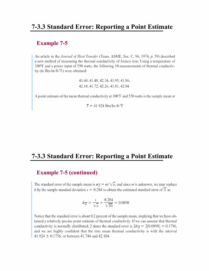
Example 7-5
7-3.3 Standard Error: Reporting a Point Estimate
Example 7-5 (continued)

7-3.4 Mean Square Error of an Estimator
7-3.4 Mean Square Error of an Estimator
Figure 7-6 A biased estimator that has smaller variance
than the unbiased estimator 1
!̂.ˆ2
!

7-4 Methods of Point Estimation
•! Problem: To find p=P(heads) for a biased coin.
•! Procedure: Flip the coin n times.
•! Data (a random sample) : X1, X2, …,Xn
–! where Xi=1 or 0 if the ith outcome is heads or tails.
•! Question: How to estimate p using the data?
7-4 Methods of Point Estimation
Definition
Definition
7-4 Methods of Point Estimation
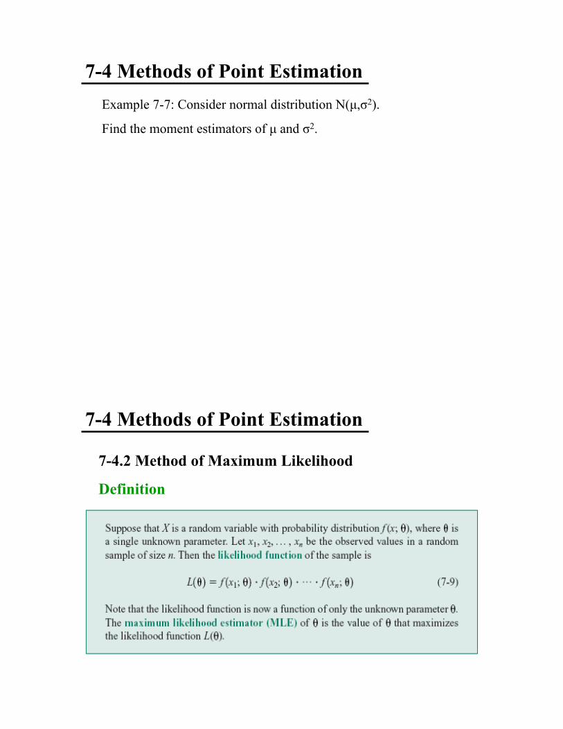
Example 7-7: Consider normal distribution N(µ,!2).
Find the moment estimators of µ and !2.
7-4 Methods of Point Estimation
7-4.2 Method of Maximum Likelihood
Definition

7-4 Methods of Point Estimation
Example 7-9
7-4 Methods of Point Estimation
Example 7-9 (continued)

7-4 Methods of Point Estimation
The time to failure of an electronic module used in an automobile engine
controller is tested at an elevated temperature to accelerate the failure
mechanism. The time to failure is exponentially distributed. Eight
units are randomly selected and tested, resulting in the following failure
time (in hours): 11.96, 5.03, 67.40, 16.07, 31.50, 7.73, 11.10, 22.38.
Here X is exponentially distributed with parameter ".
(a)!What is the moment estimate of "?
(b)! What is the MLE estimate of "?
Examples 7-6 and 7-11
7-4 Methods of Point Estimation
Figure 7-7 Log likelihood for the exponential distribution, using the
failure time data. (a) Log likelihood with n = 8 (original data). (b)
Difference in Log likelihood if n = 8, 20, and 40.

7-4 Methods of Point Estimation
Example 7-12
7-4 Methods of Point Estimation
Example 7-12 (continued)

7-4 Methods of Point Estimation
Cramer-Rao Inequality (extra!)
!
!
Let X1,X
2,!,X
n be a random sample with pdf f (x,").
If ˆ # is an unbiased estimator of ", then
var( ˆ # ) $1
nI(")
where
I(") = E%
%"ln f (X;" )
&
' ( )
* +
2= ,E
%2
%"2ln f (X;" )
&
'
( (
)
*
+ +
is the Fisher information.
7-4 Methods of Point Estimation
Properties of the Maximum Likelihood Estimator

7-4 Methods of Point Estimation
The Invariance Property
7-4 Methods of Point Estimation
Complications in Using Maximum Likelihood Estimation
•! It is not always easy to maximize the likelihood
function because the equation(s) obtained from dL(!)/
d! = 0 may be difficult to solve.
•! It may not always be possible to use calculus
methods directly to determine the maximum of L(!).
•! See Example 7-14.
8-1 Introduction
•! In the previous chapter we illustrated how a parameter
can be estimated from sample data. However, it is important to understand how good is the estimate obtained.
•! Bounds that represent an interval of plausible values for
a parameter are an example of an interval estimate.
•! Three types of intervals will be presented:
•! Confidence intervals
•! Prediction intervals
•! Tolerance intervals
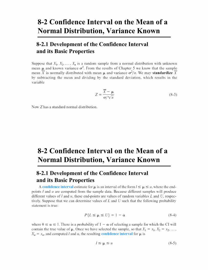
8-2.1 Development of the Confidence Interval
and its Basic Properties
8-2 Confidence Interval on the Mean of a
Normal Distribution, Variance Known
8-2.1 Development of the Confidence Interval
and its Basic Properties
8-2 Confidence Interval on the Mean of a
Normal Distribution, Variance Known

8-2.1 Development of the Confidence Interval and its
Basic Properties
•! The endpoints or bounds l and u are called lower- and upper-
confidence limits, respectively.
•! Since Z follows a standard normal distribution, we can write:
8-2 Confidence Interval on the Mean of a
Normal Distribution, Variance Known
8-2.1 Development of the Confidence Interval and its
Basic Properties
Definition
8-2 Confidence Interval on the Mean of a
Normal Distribution, Variance Known

Example 8-1
8-2 Confidence Interval on the Mean of a
Normal Distribution, Variance Known
Interpreting a Confidence Interval
•! The confidence interval is a random interval
•! The appropriate interpretation of a confidence interval
(for example on µ) is: The observed interval [l, u]
brackets the true value of µ, with confidence 100(1-!).
•! Examine Figure 8-1 on the next slide.
•! Simulation on CI
8-2 Confidence Interval on the Mean of a
Normal Distribution, Variance Known

8-2 Confidence Interval on the Mean of a
Normal Distribution, Variance Known
Figure 8-1 Repeated construction of a confidence interval for µ.
Confidence Level and Precision of Error
The length of a confidence interval is a measure of the
precision of estimation.
8-2 Confidence Interval on the Mean of a
Normal Distribution, Variance Known
Figure 8-2 Error in estimating µ with . x

8-2.2 Choice of Sample Size
8-2 Confidence Interval on the Mean of a
Normal Distribution, Variance Known
Example 8-2
8-2 Confidence Interval on the Mean of a
Normal Distribution, Variance Known
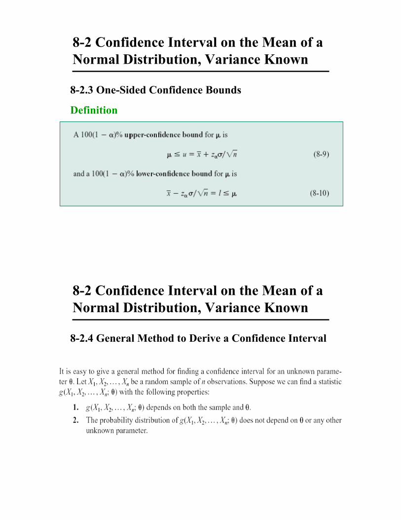
8-2.3 One-Sided Confidence Bounds
Definition
8-2 Confidence Interval on the Mean of a
Normal Distribution, Variance Known
8-2.4 General Method to Derive a Confidence Interval
8-2 Confidence Interval on the Mean of a
Normal Distribution, Variance Known

8-2.4 General Method to Derive a Confidence Interval
8-2 Confidence Interval on the Mean of a
Normal Distribution, Variance Known
8-2.4 General Method to Derive a Confidence Interval
8-2 Confidence Interval on the Mean of a
Normal Distribution, Variance Known

8-2.5 A Large-Sample Confidence Interval for µ
Definition
8-2 Confidence Interval on the Mean of a
Normal Distribution, Variance Known
Example 8-4
8-2 Confidence Interval on the Mean of a
Normal Distribution, Variance Known

Example 8-4 (continued)
8-2 Confidence Interval on the Mean of a
Normal Distribution, Variance Known
Figure 8-3 Mercury concentration in largemouth bass
(a) Histogram. (b) Normal probability plot
Example 8-4 (continued)
8-2 Confidence Interval on the Mean of a
Normal Distribution, Variance Known

A General Large Sample Confidence Interval
8-2 Confidence Interval on the Mean of a
Normal Distribution, Variance Known
8-3.1 The t distribution
8-3 Confidence Interval on the Mean of a
Normal Distribution, Variance Unknown

8-3.1 The t distribution
8-3 Confidence Interval on the Mean of a
Normal Distribution, Variance Unknown
Figure 8-4 Probability density functions of several t
distributions.
8-3.1 The t distribution
8-3 Confidence Interval on the Mean of a
Normal Distribution, Variance Unknown
Figure 8-5 Percentage points of the t distribution.

8-3.2 The t Confidence Interval on µ
8-3 Confidence Interval on the Mean of a
Normal Distribution, Variance Unknown
One-sided confidence bounds on the mean are found by replacing
t!/2,n-1 in Equation 8-18 with t !,n-1.
Example 8-5
8-3 Confidence Interval on the Mean of a
Normal Distribution, Variance Unknown

8-3 Confidence Interval on the Mean of a
Normal Distribution, Variance Unknown
Figure 8-6/8-7 Box and Whisker plot and Normal probability
plot for the load at failure data in Example 8-5.
Definition
8-4 Confidence Interval on the Variance and
Standard Deviation of a Normal Distribution

8-4 Confidence Interval on the Variance and
Standard Deviation of a Normal Distribution
Figure 8-8 Probability
density functions of
several "2 distributions.
Definition
8-4 Confidence Interval on the Variance and
Standard Deviation of a Normal Distribution

One-Sided Confidence Bounds
8-4 Confidence Interval on the Variance and
Standard Deviation of a Normal Distribution
Example 8-6
8-4 Confidence Interval on the Variance and
Standard Deviation of a Normal Distribution

Normal Approximation for Binomial Proportion
8-5 A Large-Sample Confidence Interval
For a Population Proportion
The quantity is called the standard error of the point
estimator .
npp /)1( !
P̂
8-5 A Large-Sample Confidence Interval
For a Population Proportion

Example 8-7
8-5 A Large-Sample Confidence Interval
For a Population Proportion
Choice of Sample Size
The sample size for a specified value E is given by
8-5 A Large-Sample Confidence Interval
For a Population Proportion
An upper bound on n is given by

Example 8-8
8-5 A Large-Sample Confidence Interval
For a Population Proportion
One-Sided Confidence Bounds
8-5 A Large-Sample Confidence Interval
For a Population Proportion

8-6 Guidelines for Constructing
Confidence Intervals
8-7.1 Prediction Interval for Future Observation
8-7 Tolerance and Prediction Intervals
The prediction interval for Xn+1 will always be longer than the
confidence interval for µ.

Example 8-9
8-7 Tolerance and Prediction
Intervals
8-7 Tolerance and Prediction
Intervals
8-7.2 Tolerance Interval for a Normal Distribution

Definition
8-7 Tolerance and Prediction
Intervals
8-7.2 Tolerance Interval for a Normal Distribution
8-7 Tolerance and Prediction
Intervals
Simulation on Tolerance Intervals

9-3.4 Likelihood ratio test
Neyman-Pearson lemma
9-1 Hypothesis Testing
9-1.1 Statistical Hypotheses
Definition
Statistical hypothesis testing and confidence interval
estimation of parameters are the fundamental methods
used at the data analysis stage of a comparative
experiment, in which the engineer is interested, for
example, in comparing the mean of a population to a
specified value.

9-1 Hypothesis Testing
9-1.1 Statistical Hypotheses
For example, suppose that we are interested in the
burning rate of a solid propellant used to power aircrew
escape systems.
•! Now burning rate is a random variable that can be
described by a probability distribution.
•! Suppose that our interest focuses on the mean burning
rate (a parameter of this distribution).
•! Specifically, we are interested in deciding whether or
not the mean burning rate is 50 centimeters per second.
9-1 Hypothesis Testing
9-1.1 Statistical Hypotheses
null hypothesis
alternative hypothesis
One-sided Alternative Hypotheses
Two-sided Alternative Hypothesis

9-1 Hypothesis Testing
9-1.1 Statistical Hypotheses
Test of a Hypothesis
•! A procedure leading to a decision about a particular
hypothesis
•! Hypothesis-testing procedures rely on using the information
in a random sample from the population of interest.
•! If this information is consistent with the hypothesis, then we
will conclude that the hypothesis is true; if this information is
inconsistent with the hypothesis, we will conclude that the
hypothesis is false.
9-1 Hypothesis Testing
9-1.2 Tests of Statistical Hypotheses
Figure 9-1 Decision criteria for testing H0:µ = 50 centimeters per
second versus H1:µ ! 50 centimeters per second.
9-1 Hypothesis Testing
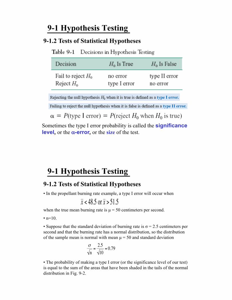
9-1.2 Tests of Statistical Hypotheses
Sometimes the type I error probability is called the significance
level, or the "-error, or the size of the test.
9-1 Hypothesis Testing
9-1.2 Tests of Statistical Hypotheses
•! In the propellant burning rate example, a type I error will occur when
when the true mean burning rate is µ = 50 centimeters per second.
•! n=10.
•! Suppose that the standard deviation of burning rate is ! = 2.5 centimeters per
second and that the burning rate has a normal distribution, so the distribution
of the sample mean is normal with mean µ = 50 and standard deviation
•! The probability of making a type I error (or the significance level of our test)
is equal to the sum of the areas that have been shaded in the tails of the normal
distribution in Fig. 9-2.
!
x < 48.5 or x > 51.5
!
"
n=
2.5
10= 0.79

9-1 Hypothesis Testing
9-1.2 Tests of Statistical Hypotheses
9-1 Hypothesis Testing

9-1 Hypothesis Testing
Figure 9-3 The
probability of type II
error when µ = 52 and n = 10.
9-1 Hypothesis Testing

9-1 Hypothesis Testing
Figure 9-4 The
probability of type II
error when µ = 50.5 and n = 10.
9-1 Hypothesis Testing

9-1 Hypothesis Testing
Figure 9-5 The
probability of type II
error when µ = 52 and n = 16.
9-1 Hypothesis Testing

9-1 Hypothesis Testing
1.! The size of the critical region, and consequently the probability of a
type I error ", can always be reduced by appropriate selection of the
critical values.
2.! Type I and type II errors are related. A decrease in the probability of
one type of error always results in an increase in the probability of
the other, provided that the sample size n does not change.
3.! An increase in sample size reduces #, provided that " is held
constant.
4.! When the null hypothesis is false, # increases as the true value of the
parameter approaches the value hypothesized in the null hypothesis.
The value of # decreases as the difference between the true mean and
the hypothesized value increases.
9-1 Hypothesis Testing

9-1 Hypothesis Testing
Definition
•! The power is computed as 1 - #, and power can be interpreted as
the probability of correctly rejecting a false null hypothesis. We
often compare statistical tests by comparing their power properties.
•! For example, consider the propellant burning rate problem when
we are testing H 0 : µ = 50 centimeters per second against H 1 : µ not
equal 50 centimeters per second . Suppose that the true value of the
mean is µ = 52. When n = 10, we found that # = 0.2643, so the
power of this test is 1 - # = 1 - 0.2643 = 0.7357 when µ = 52.
9-1 Hypothesis Testing
9-1.3 One-Sided and Two-Sided Hypotheses
Two-Sided Test:
One-Sided Tests:
Rejecting H0 is a strong conclusion.

9-1 Hypothesis Testing
Example 9-1
9-1 Hypothesis Testing
9-1.4 P-Values in Hypothesis Tests
P-value = P (test statistic will take on a value that is at least as
extreme as the observed value when the null hypothesis H0 is true)
Decision rule:
•! If P-value > ! , fail to reject H0 at significance level !;
•! If P-value < ! , reject H0 at significance level !.

9-1 Hypothesis Testing
9-1.4 P-Values in Hypothesis Tests
9-1 Hypothesis Testing
9-1.4 P-Values in Hypothesis Tests
9-1 Hypothesis Testing
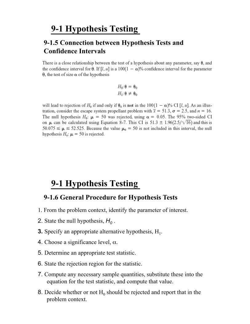
9-1.5 Connection between Hypothesis Tests and
Confidence Intervals
9-1 Hypothesis Testing
9-1.6 General Procedure for Hypothesis Tests
1. From the problem context, identify the parameter of interest.
2. State the null hypothesis, H0 .
3. Specify an appropriate alternative hypothesis, H1.
4. Choose a significance level, ".
5. Determine an appropriate test statistic.
6. State the rejection region for the statistic.
7. Compute any necessary sample quantities, substitute these into the
equation for the test statistic, and compute that value.
8. Decide whether or not H0 should be rejected and report that in the
problem context.
9-2 Tests on the Mean of a Normal
Distribution, Variance Known
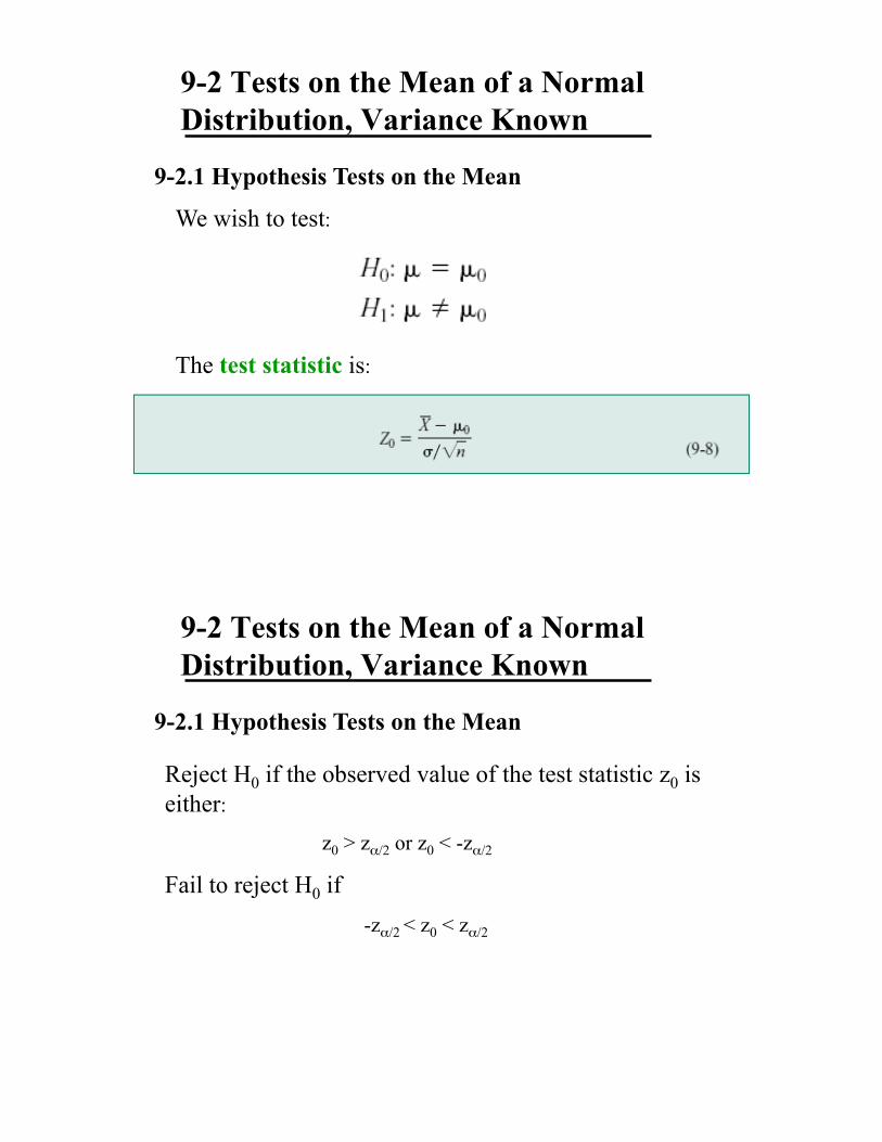
9-2.1 Hypothesis Tests on the Mean
We wish to test:
The test statistic is:
9-2 Tests on the Mean of a Normal
Distribution, Variance Known
9-2.1 Hypothesis Tests on the Mean
Reject H0 if the observed value of the test statistic z0 is
either:
z0 > z"/2 or z0 < -z"/2
Fail to reject H0 if
-z"/2 < z0 < z"/2

9-2 Tests on the Mean of a Normal
Distribution, Variance Known
9-2 Tests on the Mean of a Normal
Distribution, Variance Known
Example 9-2

9-2 Tests on the Mean of a Normal
Distribution, Variance Known
Example 9-2
9-2 Tests on the Mean of a Normal
Distribution, Variance Known
Example 9-2

9-2 Tests on the Mean of a Normal
Distribution, Variance Known
9-2.1 Hypothesis Tests on the Mean
9-2 Tests on the Mean of a Normal
Distribution, Variance Known
9-2.1 Hypothesis Tests on the Mean (Continued)

9-2 Tests on the Mean of a Normal
Distribution, Variance Known
9-2.1 Hypothesis Tests on the Mean (Continued)
The notation on p. 307 includes n-1, which is wrong.
9-2 Tests on the Mean of a Normal
Distribution, Variance Known
P-Values in Hypothesis Tests

9-2 Tests on the Mean of a Normal
Distribution, Variance Known
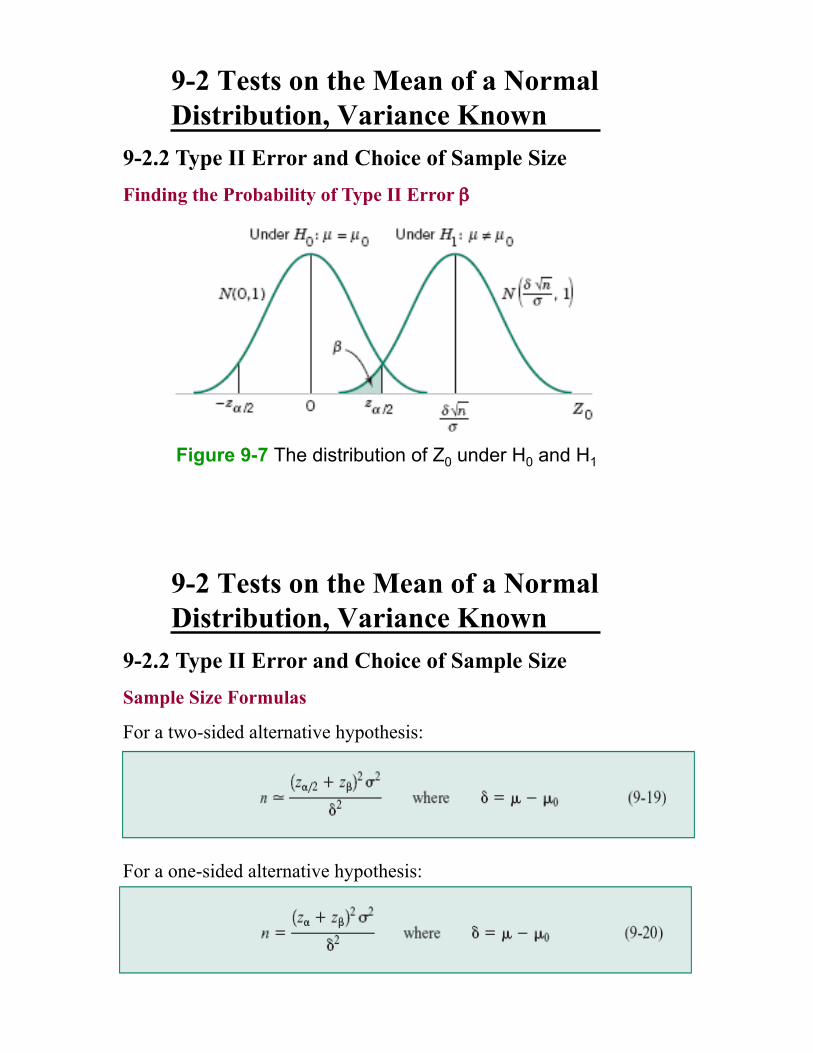
9-2.2 Type II Error and Choice of Sample Size
Finding the Probability of Type II Error #
9-2 Tests on the Mean of a Normal
Distribution, Variance Known
9-2.2 Type II Error and Choice of Sample Size
Finding the Probability of Type II Error #
# = P(type II error) = P(failing to reject H0 when it is false)
9-2 Tests on the Mean of a Normal
Distribution, Variance Known
9-2.2 Type II Error and Choice of Sample Size
Finding the Probability of Type II Error #
Figure 9-7 The distribution of Z0 under H0 and H1
9-2 Tests on the Mean of a Normal
Distribution, Variance Known
9-2.2 Type II Error and Choice of Sample Size
Sample Size Formulas
For a two-sided alternative hypothesis:
For a one-sided alternative hypothesis:

9-2 Tests on the Mean of a Normal
Distribution, Variance Known
Example 9-3
9-2 Tests on the Mean of a Normal
Distribution, Variance Known
9-2.2 Type II Error and Choice of Sample Size
Using Operating Characteristic Curves

9-2 Tests on the Mean of a Normal
Distribution, Variance Known
9-2.2 Type II Error and Choice of Sample Size
Using Operating Characteristic Curves
9-2 Tests on the Mean of a Normal
Distribution, Variance Known
Example 9-4
9-2 Tests on the Mean of a Normal
Distribution, Variance Known
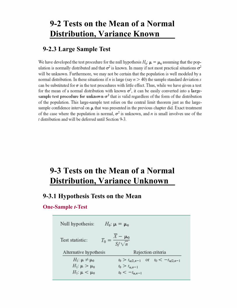
9-2.3 Large Sample Test
9-3 Tests on the Mean of a Normal
Distribution, Variance Unknown
9-3.1 Hypothesis Tests on the Mean
One-Sample t-Test

9-3 Tests on the Mean of a Normal
Distribution, Variance Unknown
9-3.1 Hypothesis Tests on the Mean
Figure 9-9 The reference distribution for H0: µ = µ0 with critical
region for (a) H1: µ ! µ0 , (b) H1: µ > µ0, and (c) H1: µ < µ0.
9-3 Tests on the Mean of a Normal
Distribution, Variance Unknown
Example 9-6

9-3 Tests on the Mean of a Normal
Distribution, Variance Unknown
Example 9-6
9-3 Tests on the Mean of a Normal
Distribution, Variance Unknown
Example 9-6
Figure 9-10
Normal probability
plot of the coefficient of
restitution data
from Example 9-6.

9-3 Tests on the Mean of a Normal
Distribution, Variance Unknown
Example 9-6
9-3 Tests on the Mean of a Normal
Distribution, Variance Unknown
9-3.2 P-value for a t-Test
The P-value for a t-test is just the smallest level of significance
at which the null hypothesis would be rejected.
Notice that t0 = 2.72 in Example 9-6, and that this is between two
tabulated values, 2.624 and 2.977. Therefore, the P-value must be
between 0.01 and 0.005. These are effectively the upper and lower
bounds on the P-value.

9-3 Tests on the Mean of a Normal
Distribution, Variance Unknown
9-3.3 Type II Error and Choice of Sample Size
The type II error of the two-sided alternative (for example)
would be
where T’0 denotes a noncentral t random variable.
9-3 Tests on the Mean of a Normal
Distribution, Variance Unknown
Example 9-7

9-3.4 Likelihood Ratio Test (extra!)
9-3.4 Likelihood Ratio Test (extra!)

9-3.4 Likelihood Ratio Test (extra!) •! Neyman-Pearson Lemma:
Likelihood-ratio test is the most powerful test of a specified value " when testing two simple hypotheses.#
•! simple hypotheses #
H0: !=!0 and H1: !=!1
9-3.4 Likelihood Ratio Test (extra!)

9-3.4 Likelihood Ratio Test (extra!)
9-3.4 Likelihood Ratio Test (extra!)

9-4 Hypothesis Tests on the Variance and
Standard Deviation of a Normal Distribution
9-4.1 Hypothesis Test on the Variance
9-4 Hypothesis Tests on the Variance and
Standard Deviation of a Normal Distribution
9-4.1 Hypothesis Test on the Variance

9-4 Hypothesis Tests on the Variance and
Standard Deviation of a Normal Distribution
9-4.1 Hypothesis Test on the Variance
9-4 Hypothesis Tests on the Variance and
Standard Deviation of a Normal Distribution
9-4.1 Hypothesis Test on the Variance

9-4 Hypothesis Tests on the Variance and
Standard Deviation of a Normal Distribution
Example 9-8
9-4 Hypothesis Tests on the Variance and
Standard Deviation of a Normal Distribution
Example 9-8

9-4 Hypothesis Tests on the Variance and
Standard Deviation of a Normal Distribution
9-4.2 Type II Error and Choice of Sample Size
Operating characteristic curves are provided in
•! Charts VII(i) and VII(j) for the two-sided alternative
•! Charts VII(k) and VII(l) for the upper tail alternative
•! Charts VII(m) and VII(n) for the lower tail alternative
9-4 Hypothesis Tests on the Variance and
Standard Deviation of a Normal Distribution
Example 9-9

9-5 Tests on a Population Proportion
9-5.1 Large-Sample Tests on a Proportion
Many engineering decision problems include hypothesis testing
about p.
An appropriate test statistic is
9-5 Tests on a Population Proportion
Example 9-10

9-5 Tests on a Population Proportion
Example 9-10
9-5 Tests on a Population Proportion
Another form of the test statistic Z0 is
or
Think about: What are the distribution of Z0 under H0 and H1?

9-5 Tests on a Population Proportion
9-5.2 Type II Error and Choice of Sample Size
For a two-sided alternative
If the alternative is p < p0
If the alternative is p > p0
9-5 Tests on a Population Proportion
9-5.3 Type II Error and Choice of Sample Size
For a two-sided alternative
For a one-sided alternative

9-5 Tests on a Population Proportion
Example 9-11
9-5 Tests on a Population Proportion
Example 9-11

9-7 Testing for Goodness of Fit
•! The test is based on the chi-square distribution.
•! Assume there is a sample of size n from a population whose
probability distribution is unknown.
•! Arrange n observations in a frequency histogram.
•! Let Oi be the observed frequency in the ith class interval.
•! Let Ei be the expected frequency in the ith class interval.
The test statistic is
which has approximately chi-square distribution with df=k-p-1.
Example 9-12
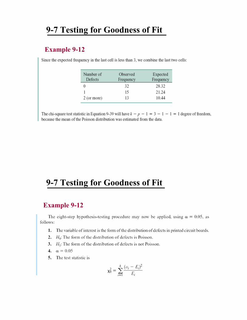
9-7 Testing for Goodness of Fit

9-7 Testing for Goodness of Fit
Example 9-12
9-7 Testing for Goodness of Fit
Example 9-12
9-7 Testing for Goodness of Fit
Example 9-12
9-7 Testing for Goodness of Fit
Example 9-12

9-7 Testing for Goodness of Fit
Example 9-12
9-8 Contingency Table Tests
Many times, the n elements of a sample from a
population may be classified according to two different
criteria. It is then of interest to know whether the two
methods of classification are statistically independent;

9-8 Contingency Table Tests
9-8 Contingency Table Tests
9-8 Contingency Table Tests
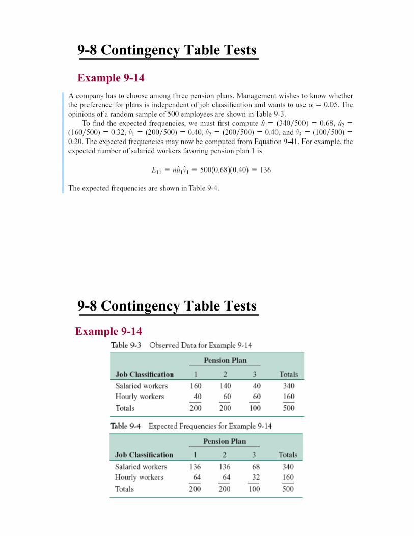
Example 9-14
9-8 Contingency Table Tests
Example 9-14

9-8 Contingency Table Tests
Example 9-14
9-8 Contingency Table Tests
Example 9-14

10-1 Introduction

Figure 10-1 Two independent populations.
10-1 Introduction
10-2 Inference for a Difference in Means
of Two Normal Distributions, Variances
Known
Assumptions

10-2 Inference for a Difference in Means
of Two Normal Distributions, Variances
Known
10-2 Inference for a Difference in Means
of Two Normal Distributions, Variances
Known
10-2.1 Hypothesis Tests for a Difference in Means,
Variances Known
10-2 Inference for a Difference in Means
of Two Normal Distributions, Variances
Known
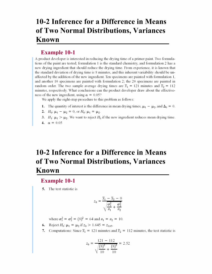
Example 10-1
10-2 Inference for a Difference in Means
of Two Normal Distributions, Variances
Known
Example 10-1

10-2 Inference for a Difference in Means
of Two Normal Distributions, Variances
Known
Example 10-1
10-2 Inference for a Difference in Means
of Two Normal Distributions, Variances
Known
10-2.2 Type II Error and Choice of Sample Size
•! Use of Operating Characteristic Curves
•! Chart VII(a)-(d)
•! Identical to 9-2.2 except

10-2 Inference for a Difference in Means
of Two Normal Distributions, Variances
Known
10-2.3 Confidence Interval on a Difference in Means,
Variances Known
Definition
10-2 Inference for a Difference in Means
of Two Normal Distributions, Variances
Known
Example 10-4

10-2 Inference for a Difference in Means
of Two Normal Distributions, Variances
Known
Example 10-4
10-2 Inference for a Difference in Means
of Two Normal Distributions, Variances
Known
One-Sided Confidence Bounds
Upper Confidence Bound
Lower Confidence Bound

10-3 Inference for a Difference in Means
of Two Normal Distributions, Variances
Unknown
10-3.1 Hypotheses Tests for a Difference in Means,
Variances Unknown
We wish to test:
Case 1:
Case 2:
10-3 Inference for a Difference in Means
of Two Normal Distributions, Variances
Unknown
The pooled estimator of !2:
Case 1:
The pooled estimator is an unbiased estimator of !2

10-3 Inference for a Difference in Means
of Two Normal Distributions, Variances
Unknown
Case 1:
10-3 Inference for a Difference in Means
of Two Normal Distributions, Variances
Unknown
Definition: The Two-Sample or Pooled t-Test*

10-3 Inference for a Difference in Means
of Two Normal Distributions, Variances
Unknown
Example 10-5
10-3 Inference for a Difference in Means
of Two Normal Distributions, Variances
Unknown

Figure 10-2 Normal probability plot and comparative box plot for
the catalyst yield data in Example 10-5. (a) Normal probability
plot, (b) Box plots.
10-3 Inference for a Difference in Means
of Two Normal Distributions, Variances
Unknown
10-3 Inference for a Difference in Means
of Two Normal Distributions, Variances
Unknown
Example 10-5

10-3 Inference for a Difference in Means
of Two Normal Distributions, Variances
Unknown
Example 10-5
10-3 Inference for a Difference in Means
of Two Normal Distributions, Variances
Unknown
Case 2:
is distributed approximately as t with degrees of freedom given by
10-3 Inference for a Difference in Means
of Two Normal Distributions, Variances
Unknown
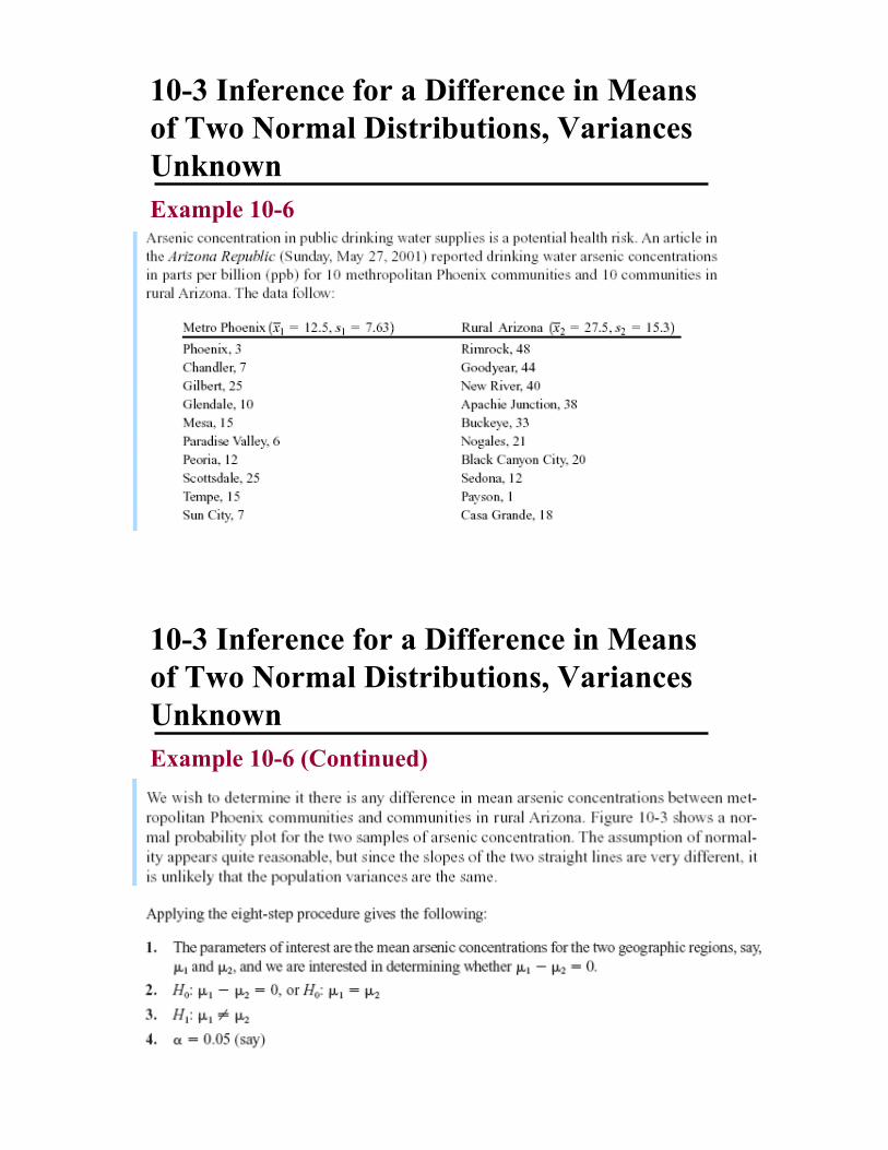
Example 10-6
10-3 Inference for a Difference in Means
of Two Normal Distributions, Variances
Unknown
Example 10-6 (Continued)

10-3 Inference for a Difference in Means
of Two Normal Distributions, Variances
Unknown
Example 10-6 (Continued)
Figure 10-3 Normal
probability plot of the
arsenic concentration data from Example 10-6.
10-3 Inference for a Difference in Means
of Two Normal Distributions, Variances
Unknown
Example 10-6 (Continued)

10-3 Inference for a Difference in Means
of Two Normal Distributions, Variances
Unknown
Example 10-6 (Continued)
10-3.3 Confidence Interval on the Difference in Means,
Variance Unknown
Case 1:

10-3.3 Confidence Interval on the Difference in Means,
Variance Unknown
Case 2:
•! A special case of the two-sample t-tests of Section
10-3 occurs when the observations on the two
populations of interest are collected in pairs.
•! Each pair of observations, say (X1j , X2j ), is taken
under homogeneous conditions, but these conditions
may change from one pair to another.
•! The test procedure consists of analyzing the
differences between two observations from each pair.
10-4 Paired t-Test

The Paired t-Test
10-4 Paired t-Test
Example 10-9
10-4 Paired t-Test

Example 10-9
10-4 Paired t-Test
Example 10-9
10-4 Paired t-Test
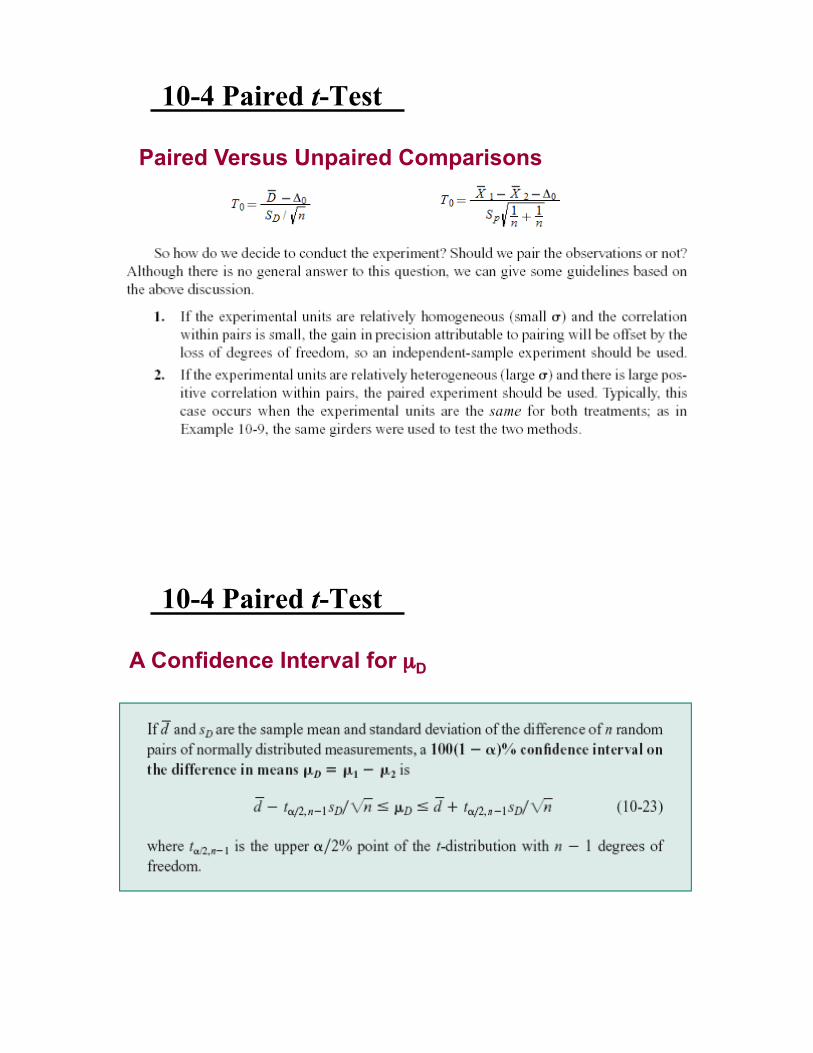
Paired Versus Unpaired Comparisons
10-4 Paired t-Test
A Confidence Interval for µD
10-4 Paired t-Test

10-5.1 The F distribution
11-1 Empirical Models
•! Many problems in engineering and science involve
exploring the relationships between two or more
variables.
•! Regression analysis is a statistical technique that is
very useful for these types of problems.
•! For example, in a chemical process, suppose that the
yield of the product is related to the process-operating
temperature.
•! Regression analysis can be used to build a model to
predict yield at a given temperature level.

11-1 Empirical Models
11-1 Empirical Models
Based on the scatter diagram, it is probably reasonable to
assume that the mean of the random variable Y is related to x by
the following straight-line relationship:
where the slope and intercept of the line are called regression
coefficients.
The simple linear regression model is given by
where ! is the random error term.

11-1 Empirical Models
We think of the regression model as an empirical model.
Suppose that the mean and variance of ! are 0 and "2,
respectively, then
The variance of Y given x is
11-1 Empirical Models
•! The true regression model is a line of mean values:
where #1 can be interpreted as the change in the
mean of Y for a unit change in x.
•! Also, the variability of Y at a particular value of x is
determined by the error variance, "2.
•! This implies there is a distribution of Y-values at
each x and that the variance of this distribution is the
same at each x.

11-1 Empirical Models
Figure 11-2 The distribution of Y for a given value of
x for the oxygen purity-hydrocarbon data.
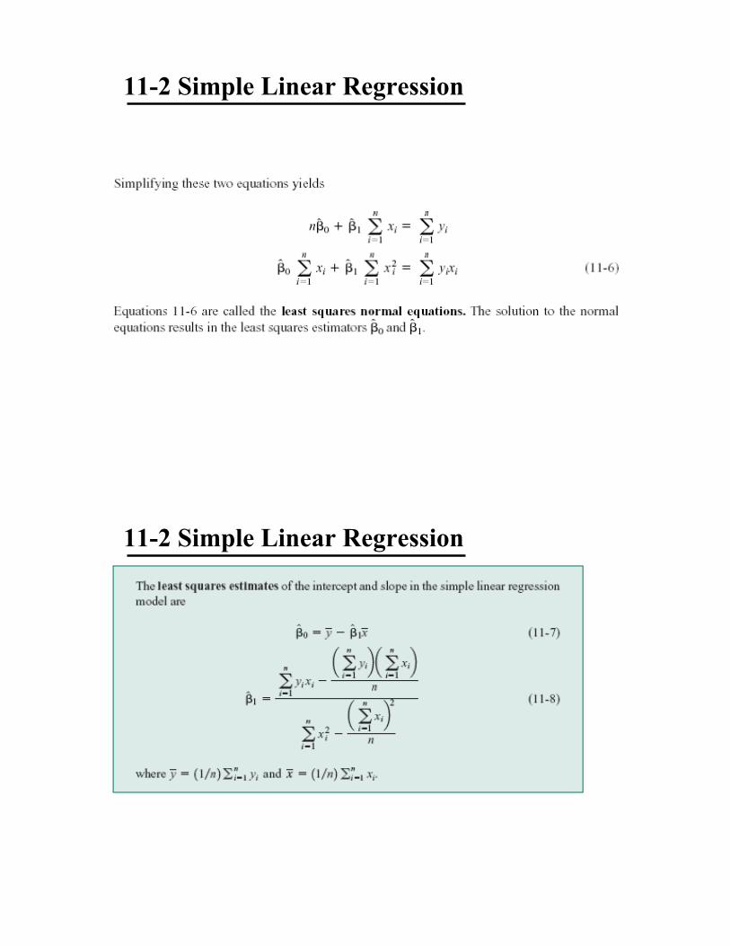
11-2 Simple Linear Regression
•! The case of simple linear regression considers
a single regressor or predictor x and a
dependent or response variable Y.
•! The expected value of Y at each level of x is a
random variable:
•! We assume that each observation, Y, can be
described by the model

11-2 Simple Linear Regression
•! Suppose that we have n pairs of observations
(x1, y1), (x2, y2), …, (xn, yn).
Figure 11-3
Deviations of the
data from the estimated
regression model.
11-2 Simple Linear Regression
•! The method of least squares is used to
estimate the parameters, #0 and #1 by minimizing
the sum of the squares of the vertical deviations in
Figure 11-3.
Figure 11-3
Deviations of the
data from the estimated
regression model.

11-2 Simple Linear Regression
•! Using Equation 11-2, the n observations in the
sample can be expressed as
•! The sum of the squares of the deviations of the
observations from the true regression line is
11-2 Simple Linear Regression
11-2 Simple Linear Regression
11-2 Simple Linear Regression

11-2 Simple Linear Regression
11-2 Simple Linear Regression
Notation

11-2 Simple Linear Regression
Example 11-1
11-2 Simple Linear Regression
Example 11-1

11-2 Simple Linear Regression
Example 11-1
Figure 11-4 Scatter
plot of oxygen
purity y versus hydrocarbon level x
and regression
model ! = 74.20 +
14.97x.

11-2 Simple Linear Regression
Estimating "2
The error sum of squares is
It can be shown that the expected value of the
error sum of squares is E(SSE) = (n – 2)"2.
11-2 Simple Linear Regression
Estimating "2
An unbiased estimator of "2 is
where SSE can be easily computed using
!
where SST = (yi " y i=1
n
# )2
= yi
2 " ny 2
= Syy
i=1
n
#

11-3 Properties of the Least Squares
Estimators
•! Slope Properties
•! Intercept Properties
11-4 Hypothesis Tests in Simple Linear
Regression
11-4.1 Use of t-Tests
Suppose we wish to test
An appropriate test statistic would be

11-4 Hypothesis Tests in Simple Linear
Regression
Assumptions:
To test hypotheses about the slope and intercept of the regression
model, we must make the additional assumption that the error
component in the model, !, is normally distributed.
Thus, the complete assumptions are that the errors are normally
and independently distributed with mean zero and variance "2,
abbreviated NID(0, "2).
11-4 Hypothesis Tests in Simple Linear
Regression
11-4.1 Use of t-Tests
We would reject the null hypothesis if
The test statistic could also be written as:

11-4.1 Use of t-Tests
Suppose we wish to test
An appropriate test statistic would be
We would reject the null hypothesis if
11-4 Hypothesis Tests in Simple Linear
Regression
11-4.1 Use of t-Tests
An important special case of the hypotheses of
Equation 11-18 is
These hypotheses relate to the significance of regression.
Failure to reject H0 is equivalent to concluding that there
is no linear relationship between x and Y.

11-4 Hypothesis Tests in Simple Linear
Regression
Figure 11-5 The hypothesis H0: #1 = 0 is not rejected.
11-4 Hypothesis Tests in Simple Linear
Regression
Figure 11-6 The hypothesis H0: #1 = 0 is rejected.

11-4 Hypothesis Tests in Simple Linear
Regression
Example 11-2
> dat=read.table("table11-1.txt", h=T)!> g=lm(y~x, dat)!> summary(g)!Coefficients:! Estimate Std. Error t value Pr(>|t|) !(Intercept) 74.283 1.593 46.62 < 2e-16 ***!x 14.947 1.317 11.35 1.23e-09 ***!
Residual standard error: 1.087 on 18 degrees of freedom!Multiple R-Squared: 0.8774, !Adjusted R-squared: 0.8706 !F-statistic: 128.9 on 1 and 18 DF, p-value: 1.227e-09 !
> anova(g)!Analysis of Variance Table!
Response: y! Df Sum Sq Mean Sq F value Pr(>F) !x 1 152.127 152.127 128.86 1.227e-09 ***!Residuals 18 21.250 1.181 !
R commands and outputs

10-5.1 The F Distribution
10-5.1 The F Distribution

10-5.1 The F Distribution
The lower-tail percentage points f 1-!,u," can be found as follows.
11-4 Hypothesis Tests in Simple Linear
Regression
11-4.2 Analysis of Variance Approach to Test
Significance of Regression
The analysis of variance identity is
Symbolically,

11-4 Hypothesis Tests in Simple Linear
Regression
11-4.2 Analysis of Variance Approach to Test
Significance of Regression
If the null hypothesis, H0: #1 = 0 is true, the statistic
follows the F1,n-2 distribution and we would reject if
f0 > f$,1,n-2.
11-4 Hypothesis Tests in Simple Linear
Regression
11-4.2 Analysis of Variance Approach to Test
Significance of Regression
The quantities, MSR and MSE are called mean squares.
Analysis of variance table:

11-4 Hypothesis Tests in Simple Linear
Regression
Example 11-3
11-4 Hypothesis Tests in Simple Linear
Regression

11-5 Confidence Intervals
11-5.1 Confidence Intervals on the Slope and Intercept
Definition
11-6 Confidence Intervals
Example 11-4

11-5 Confidence Intervals
11-5.2 Confidence Interval on the Mean Response
Definition
11-5 Confidence Intervals
Example 11-5

11-5 Confidence Intervals
11-5 Confidence Intervals
Example 11-5
Figure 11-7
Scatter diagram of
oxygen purity data from Example 11-1
with fitted
regression line and
95 percent
confidence limits on µY|x0.

11-6 Prediction of New Observations
If x0 is the value of the regressor variable of interest,
is the point estimator of the new or future value of the
response, Y0.
11-6 Prediction of New Observations
Definition

11-6 Prediction of New Observations
Example 11-6
11-6 Prediction of New Observations
Example 11-6

11-6 Prediction of New Observations
Example 11-6
Figure 11-8 Scatter
diagram of oxygen
purity data from Example 11-1 with
fitted regression line,
95% prediction limits
(outer lines) , and
95% confidence limits on µY|x0.
11-7 Adequacy of the Regression Model
•! Fitting a regression model requires several
assumptions.
1.! Errors are uncorrelated random variables with
mean zero;
2.! Errors have constant variance; and,
3.! Errors be normally distributed.
•! The analyst should always consider the validity of
these assumptions to be doubtful and conduct
analyses to examine the adequacy of the model

11-7 Adequacy of the Regression Model
11-7.1 Residual Analysis
•! The residuals from a regression model are ei = yi - !i , where yi
is an actual observation and !i is the corresponding fitted value
from the regression model.
•! Analysis of the residuals is frequently helpful in checking the
assumption that the errors are approximately normally distributed
with constant variance, and in determining whether additional
terms in the model would be useful.
11-7 Adequacy of the Regression Model
11-7.1 Residual Analysis
Figure 11-9 Patterns
for residual plots. (a)
satisfactory, (b) funnel, (c) double
bow, (d) nonlinear.
[Adapted from
Montgomery, Peck,
and Vining (2001).]
11-7 Adequacy of the Regression Model
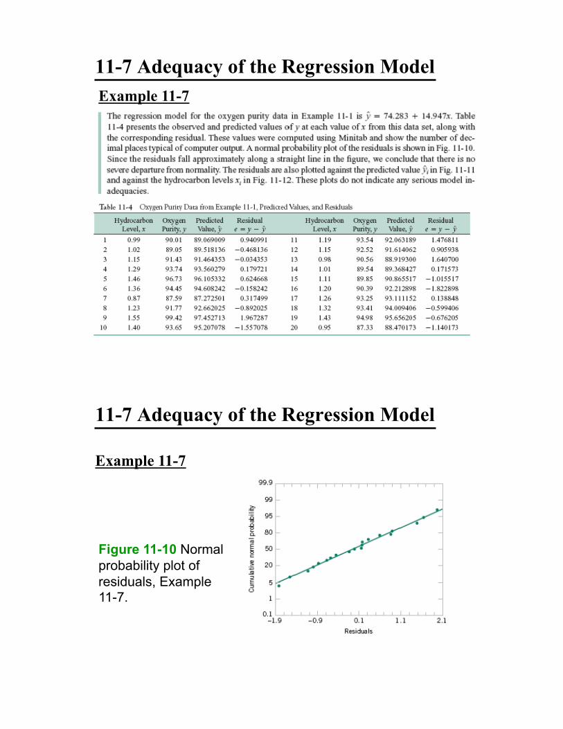
Example 11-7
11-7 Adequacy of the Regression Model
Example 11-7
Figure 11-10 Normal
probability plot of
residuals, Example 11-7.

11-7 Adequacy of the Regression Model
Example 11-7
Figure 11-11 Plot of
residuals versus
predicted oxygen purity, !, Example
11-7.
11-7 Adequacy of the Regression Model
11-7.2 Coefficient of Determination (R2)
•! The quantity
is called the coefficient of determination and is often
used to judge the adequacy of a regression model.
•! 0 % R2 % 1;
•! We often refer (loosely) to R2 as the amount of
variability in the data explained or accounted for by the
regression model.

11-7 Adequacy of the Regression Model
11-7.2 Coefficient of Determination (R2)
•! For the oxygen purity regression model,
R2 = SSR/SST
= 152.13/173.38
= 0.877
•! Thus, the model accounts for 87.7% of the
variability in the data.
11-9 Transformation and Logistic Regression

11-9 Transformation and Logistic
Regression
Example 11-9
Table 11-5 Observed Values
and Regressor Variable for
Example 11-9.
iy
ix
11-9 Transformation and Logistic
Regression

11-9 Transformation and Logistic
Regression
11-9 Transformation and Logistic
Regression

12-1 Multiple Linear Regression Models
•! Many applications of regression analysis involve
situations in which there are more than one
regressor variable.
•! A regression model that contains more than one
regressor variable is called a multiple regression
model.
12-1.1 Introduction

12-1 Multiple Linear Regression Models
•! For example, suppose that the effective life of a cutting
tool depends on the cutting speed and the tool angle. A
possible multiple regression model could be
where
Y – tool life
x1 – cutting speed
x2 – tool angle
12-1.1 Introduction
12-1 Multiple Linear Regression Models
Figure 12-1 (a) The regression plane for the model E(Y)
= 50 + 10x1 + 7x2. (b) The contour plot
12-1.1 Introduction
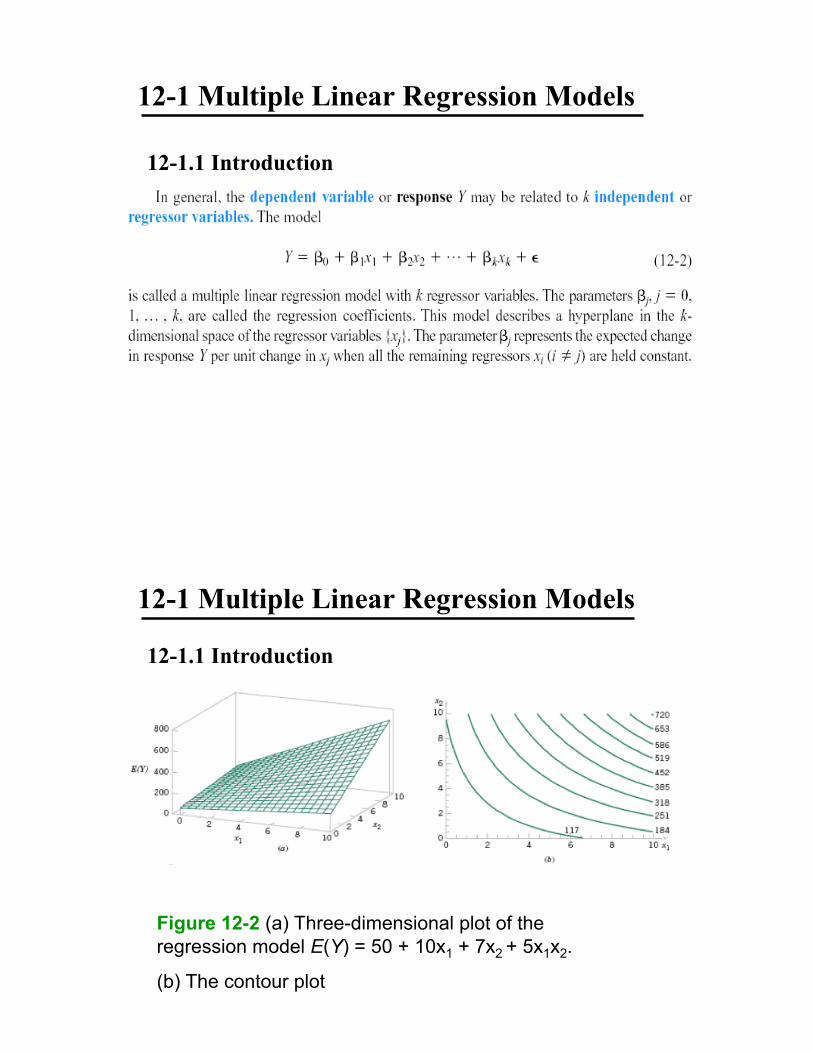
12-1 Multiple Linear Regression Models
12-1.1 Introduction
12-1 Multiple Linear Regression Models
Figure 12-2 (a) Three-dimensional plot of the
regression model E(Y) = 50 + 10x1 + 7x2 + 5x1x2.
(b) The contour plot
12-1.1 Introduction

12-1 Multiple Linear Regression Models
Figure 12-3 (a) 3-D plot of the regression model
E(Y) = 800 + 10x1 + 7x2 – 8.5x12 – 5x2
2 + 4x1x2.
(b) The contour plot
12-1.1 Introduction
12-1 Multiple Linear Regression Models
12-1.2 Least Squares Estimation of the Parameters

12-1 Multiple Linear Regression Models
12-1.2 Least Squares Estimation of the Parameters
•! The least squares function is given by
•! The least squares estimates must satisfy
12-1 Multiple Linear Regression Models
12-1.2 Least Squares Estimation of the Parameters
•! The solution to the normal Equations are the least
squares estimators of the regression coefficients.
•! The least squares normal Equations are

12-1 Multiple Linear Regression Models
12-1.3 Matrix Approach to Multiple Linear Regression
Suppose the model relating the regressors to the
response is
In matrix notation this model can be written as
12-1 Multiple Linear Regression Models
12-1.3 Matrix Approach to Multiple Linear Regression
where

12-1 Multiple Linear Regression Models
12-1.3 Matrix Approach to Multiple Linear Regression
We wish to find the vector of least squares
estimators that minimizes:
The resulting least squares estimate is
12-1 Multiple Linear Regression Models
12-1.3 Matrix Approach to Multiple Linear Regression

12-1 Multiple Linear Regression Models
Example 12-2
12-1 Multiple Linear Regression Models
Figure 12-4 Matrix of scatter plots (from Minitab) for the
wire bond pull strength data in Table 12-2.

Example 12-2
12-1 Multiple Linear Regression Models
Example 12-2

12-1 Multiple Linear Regression Models
Example 12-2
12-1 Multiple Linear Regression Models
Example 12-2

12-1 Multiple Linear Regression Models
Example 12-2

12-1 Multiple Linear Regression Models
Estimating !2
An unbiased estimator of !2 is
12-1 Multiple Linear Regression Models
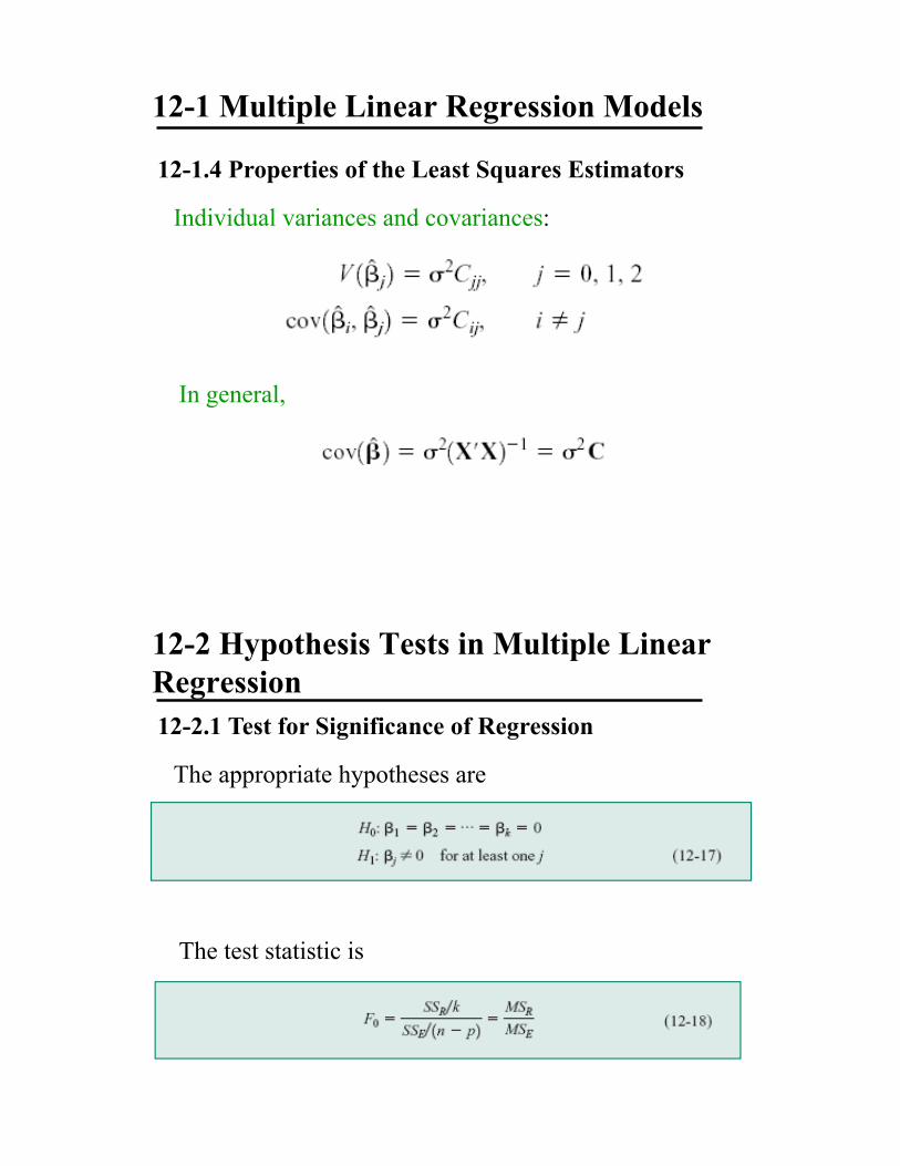
12-1.4 Properties of the Least Squares Estimators
Unbiased estimators:
Covariance Matrix:
12-1 Multiple Linear Regression Models
12-1.4 Properties of the Least Squares Estimators
Individual variances and covariances:
In general,
12-2 Hypothesis Tests in Multiple Linear
Regression
12-2.1 Test for Significance of Regression
The appropriate hypotheses are
The test statistic is

12-2 Hypothesis Tests in Multiple Linear
Regression
12-2.1 Test for Significance of Regression
12-2 Hypothesis Tests in Multiple Linear
Regression
Example 12-3

12-2 Hypothesis Tests in Multiple Linear
Regression
R2 and Adjusted R2
The coefficient of multiple determination
•! For the wire bond pull strength data, we find that R2 =
SSR/SST = 5990.7712/6105.9447 = 0.9811.
•! Thus, the model accounts for about 98% of the
variability in the pull strength response.
12-2 Hypothesis Tests in Multiple Linear
Regression
R2 and Adjusted R2
The adjusted R2 is
•! The adjusted R2 statistic penalizes the analyst for
adding terms to the model.
•! It can help guard against overfitting (including
regressors that are not really useful)

12-2 Hypothesis Tests in Multiple Linear
Regression
12-2.2 Tests on Individual Regression Coefficients and
Subsets of Coefficients
•! Reject H0 if |t0| > t"/2,n-p.
•! This is called a partial or marginal test
12-2 Hypothesis Tests in Multiple Linear
Regression
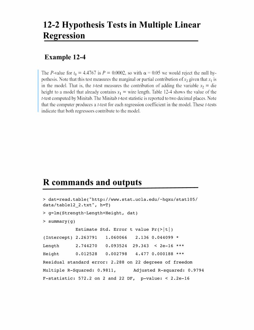
Example 12-4
12-2 Hypothesis Tests in Multiple Linear
Regression
Example 12-4
R commands and outputs
> dat=read.table("http://www.stat.ucla.edu/~hqxu/stat105/data/table12_2.txt", h=T)!
> g=lm(Strength~Length+Height, dat)!
> summary(g)!
Estimate Std. Error t value Pr(>|t|) !
(Intercept) 2.263791 1.060066 2.136 0.044099 * !
Length 2.744270 0.093524 29.343 < 2e-16 ***!
Height 0.012528 0.002798 4.477 0.000188 ***!
Residual standard error: 2.288 on 22 degrees of freedom!
Multiple R-Squared: 0.9811, !Adjusted R-squared: 0.9794 !
F-statistic: 572.2 on 2 and 22 DF, p-value: < 2.2e-16 !

13-1 Designing Engineering Experiments
Every experiment involves a sequence of activities:
1.! Conjecture – the original hypothesis that motivates the
experiment.
2.! Experiment – the test performed to investigate the
conjecture.
3.! Analysis – the statistical analysis of the data from the
experiment.
4.! Conclusion – what has been learned about the original
conjecture from the experiment. Often the experiment will
lead to a revised conjecture, and a new experiment, and so
forth.

13-2 The Completely Randomized Single-
Factor Experiment
13-2.1 An Example
13-2 The Completely Randomized Single-
Factor Experiment
13-2.1 An Example

13-2 The Completely Randomized Single-
Factor Experiment
13-2.1 An Example
•! The levels of the factor are sometimes called
treatments.
•! Each treatment has six observations or replicates.
•! The runs are run in random order.
13-2 The Completely Randomized Single-
Factor Experiment
Figure 13-1 (a) Box plots of hardwood concentration data.
(b) Display of the model in Equation 13-1 for the completely
randomized single-factor experiment
13-2.1 An Example

13-2 The Completely Randomized Single-
Factor Experiment
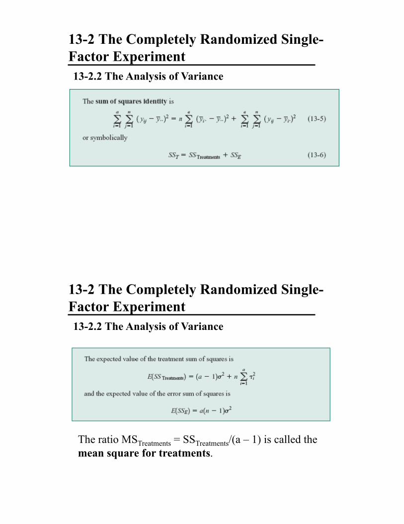
13-2.2 The Analysis of Variance
Suppose there are a different levels of a single factor
that we wish to compare. The levels are sometimes
called treatments.
13-2 The Completely Randomized Single-
Factor Experiment
13-2.2 The Analysis of Variance
We may describe the observations in Table 13-2 by the
linear statistical model:
The model could be written as

13-2 The Completely Randomized Single-
Factor Experiment
13-2.2 The Analysis of Variance
Fixed-effects Model
The treatment effects are usually defined as deviations
from the overall mean so that:
Also,
13-2 The Completely Randomized Single-
Factor Experiment
13-2.2 The Analysis of Variance
We wish to test the hypotheses:
The analysis of variance partitions the total variability
into two parts.
13-2 The Completely Randomized Single-
Factor Experiment
13-2.2 The Analysis of Variance
13-2 The Completely Randomized Single-
Factor Experiment
13-2.2 The Analysis of Variance
The ratio MSTreatments = SSTreatments/(a – 1) is called the
mean square for treatments.

13-2 The Completely Randomized Single-
Factor Experiment
13-2.2 The Analysis of Variance
The appropriate test statistic is
We would reject H0 if f0 > f!,a-1,a(n-1)
13-2 The Completely Randomized Single-
Factor Experiment
13-2.2 The Analysis of Variance
where N=na is the total number of observations.

13-2 The Completely Randomized Single-
Factor Experiment
13-2.2 The Analysis of Variance
Analysis of Variance Table
13-2 The Completely Randomized Single-
Factor Experiment
Example 13-1

13-2 The Completely Randomized Single-
Factor Experiment
Example 13-1
13-2 The Completely Randomized Single-
Factor Experiment
Example 13-1

13-2 The Completely Randomized Single-
Factor Experiment
The 95% CI on the mean of the 20% hardwood is
13-2 The Completely Randomized Single-
Factor Experiment
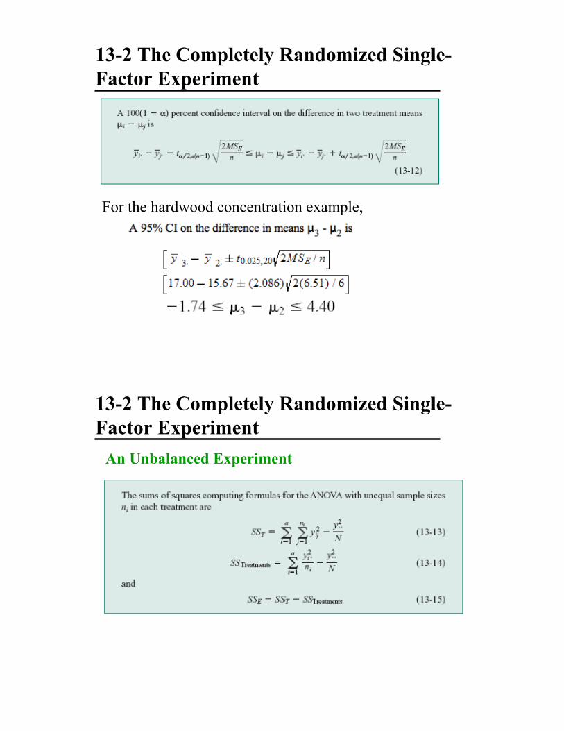
For the hardwood concentration example,
13-2 The Completely Randomized Single-
Factor Experiment
An Unbalanced Experiment

13-2 The Completely Randomized Single-
Factor Experiment
13-2.3 Multiple Comparisons Following the ANOVA
The least significant difference (LSD) is
If the sample sizes are different in each treatment:
13-2 The Completely Randomized Single-
Factor Experiment
Example 13-2

13-2 The Completely Randomized Single-
Factor Experiment Example 13-2
13-2 The Completely Randomized Single-
Factor Experiment
Example 13-2
Figure 13-2 Results of Fisher’s LSD method in Example 13-2
13-2 The Completely Randomized Single-
Factor Experiment
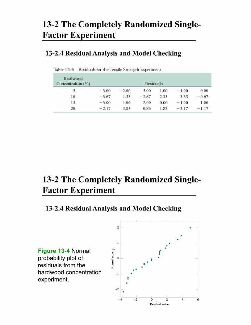
13-2.4 Residual Analysis and Model Checking
13-2 The Completely Randomized Single-
Factor Experiment
13-2.4 Residual Analysis and Model Checking
Figure 13-4 Normal
probability plot of
residuals from the hardwood concentration
experiment.

13-2 The Completely Randomized Single-
Factor Experiment
13-2.4 Residual Analysis and Model Checking
Figure 13-5 Plot of
residuals versus factor
levels (hardwood concentration).
13-2 The Completely Randomized Single-
Factor Experiment
13-2.4 Residual Analysis and Model Checking
Figure 13-6 Plot of
residuals versus

13-4 Randomized Complete Block Designs
13-4.1 Design and Statistical Analyses
The randomized block design is an extension of the
paired t-test to situations where the factor of interest has
more than two levels.
Figure 13-9 A randomized complete block design.
13-4 Randomized Complete Block Designs
13-4.1 Design and Statistical Analyses
For example, consider the situation of Example 10-9,
where two different methods were used to predict the
shear strength of steel plate girders. Say we use four
girders as the experimental units.

13-4 Randomized Complete Block Designs
13-4.1 Design and Statistical Analyses
General procedure for a randomized complete block
design:
13-4 Randomized Complete Block Designs
13-4.1 Design and Statistical Analyses
The appropriate linear statistical model:
We assume
•! treatments and blocks are initially fixed effects
•! blocks do not interact
•!

13-4 Randomized Complete Block Designs
13-4.1 Design and Statistical Analyses
We are interested in testing:
13-4 Randomized Complete Block Designs
13-4.1 Design and Statistical Analyses
The mean squares are:

13-4 Randomized Complete Block Designs
13-4.1 Design and Statistical Analyses
The expected values of these mean squares are:
13-4 Randomized Complete Block Designs
13-4.1 Design and Statistical Analyses

13-4 Randomized Complete Block Designs
Example 13-5
13-4 Randomized Complete Block Designs
Example 13-5

13-4 Randomized Complete Block Designs
Minitab Output for Example 13-5
13-4 Randomized Complete Block Designs
13-4.2 Multiple Comparisons
Fisher’s Least Significant Difference for Example 13-5
Figure 13-10 Results of Fisher’s LSD method.

13-4 Randomized Complete Block Designs
13-4.3 Residual Analysis and Model Checking
(a) Normal prob. plot of residuals (b) Residuals versus !ij
13-4 Randomized Complete Block Designs
(a) Residuals by block. (b) Residuals by treatment

14-1 Introduction
•! An experiment is a test or series of tests.
•! The design of an experiment plays a major role in
the eventual solution of the problem.
•! In a factorial experimental design, experimental
trials (or runs) are performed at all combinations of
the factor levels.
•! The analysis of variance (ANOVA) will be used as
one of the primary tools for statistical data analysis.

14-2 Factorial Experiments
Definition
14-2 Factorial Experiments
Figure 14-3 Factorial Experiment, no interaction.
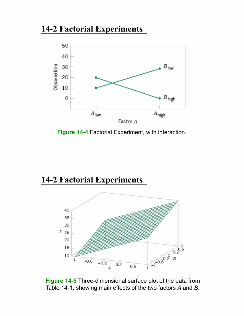
14-2 Factorial Experiments
Figure 14-4 Factorial Experiment, with interaction.
14-2 Factorial Experiments
Figure 14-5 Three-dimensional surface plot of the data from
Table 14-1, showing main effects of the two factors A and B.

14-2 Factorial Experiments
Figure 14-6 Three-dimensional surface plot of the data from
Table 14-2, showing main effects of the A and B interaction.
14-2 Factorial Experiments
Figure 14-7 Yield versus reaction time with temperature
constant at 155º F.

14-2 Factorial Experiments
Figure 14-8 Yield versus temperature with reaction time
constant at 1.7 hours.
14-2 Factorial Experiments
Figure 14-9
Optimization
experiment using the one-factor-at-a-time
method.

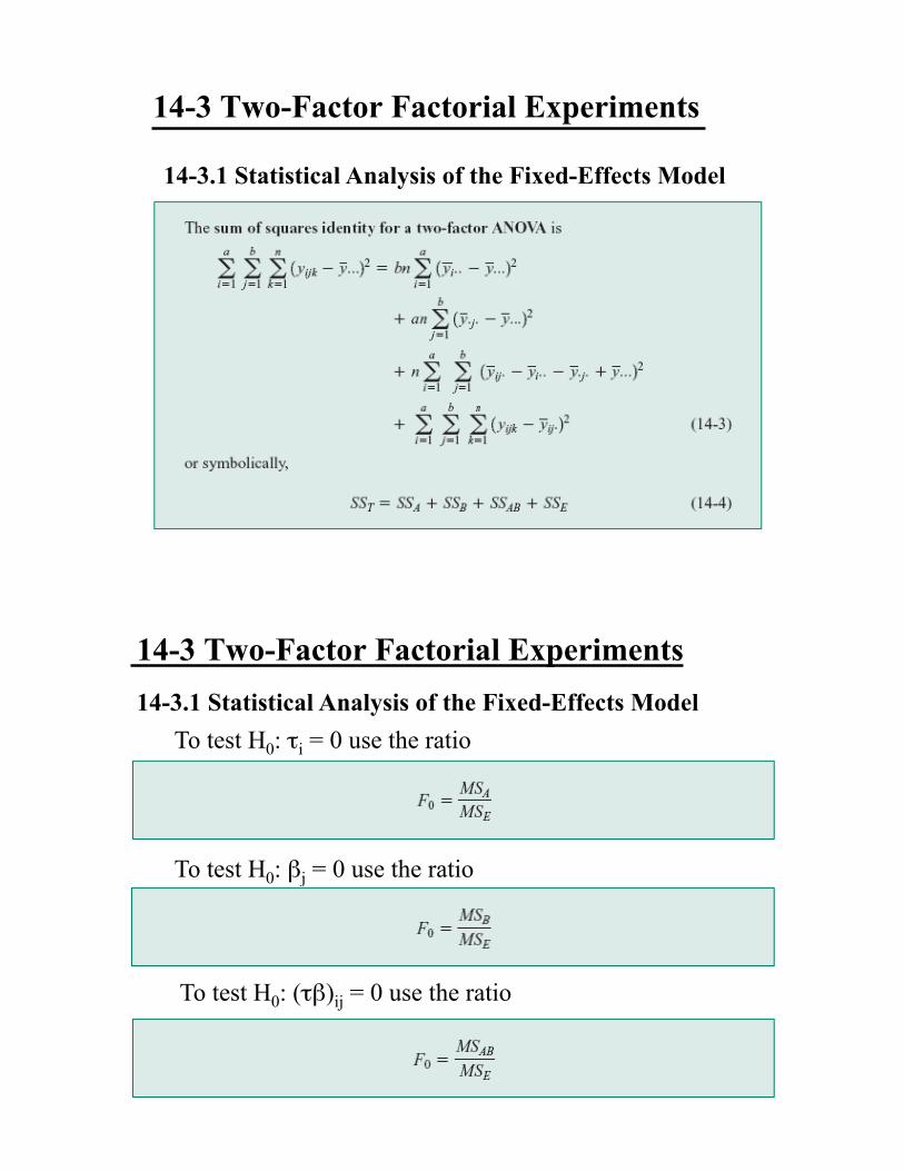
14-3 Two-Factor Factorial Experiments
14-3 Two-Factor Factorial Experiments
The observations may be described by the linear
statistical model:

14-3 Two-Factor Factorial Experiments
14-3.1 Statistical Analysis of the Fixed-Effects Model
14-3 Two-Factor Factorial Experiments
14-3.1 Statistical Analysis of the Fixed-Effects Model
14-3 Two-Factor Factorial Experiments
14-3.1 Statistical Analysis of the Fixed-Effects Model
14-3 Two-Factor Factorial Experiments
To test H0: !i = 0 use the ratio
14-3.1 Statistical Analysis of the Fixed-Effects Model
To test H0: "j = 0 use the ratio
To test H0: (!")ij = 0 use the ratio

14-3 Two-Factor Factorial Experiments
14-3.1 Statistical Analysis of the Fixed-Effects Model
Definition
14-3 Two-Factor Factorial Experiments
14-3.1 Statistical Analysis of the Fixed-Effects Model
14-3 Two-Factor Factorial Experiments
14-3.1 Statistical Analysis of the Fixed-Effects Model
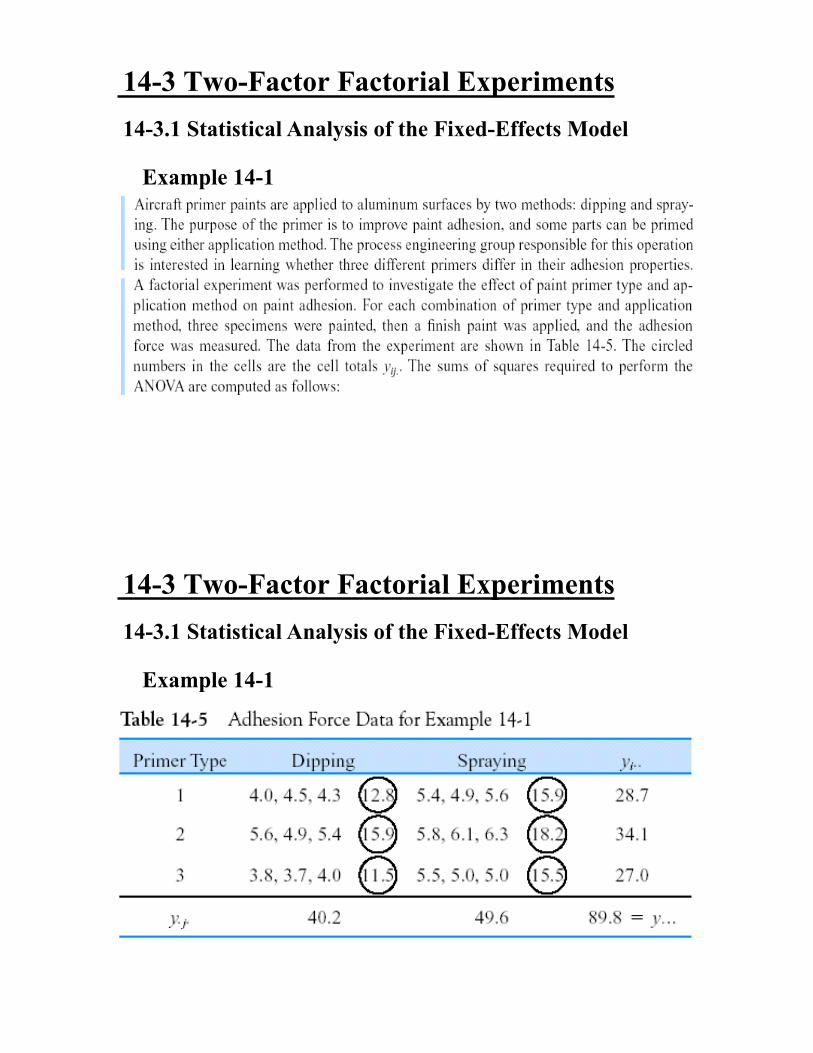
Example 14-1
14-3 Two-Factor Factorial Experiments
14-3.1 Statistical Analysis of the Fixed-Effects Model
Example 14-1

14-3 Two-Factor Factorial Experiments
14-3.1 Statistical Analysis of the Fixed-Effects Model
Example 14-1
14-3 Two-Factor Factorial Experiments
14-3.1 Statistical Analysis of the Fixed-Effects Model
Example 14-1

14-3 Two-Factor Factorial Experiments
14-3.1 Statistical Analysis of the Fixed-Effects Model
Example 14-1
14-3 Two-Factor Factorial Experiments
14-3.1 Statistical Analysis of the Fixed-Effects Model
Example 14-1

14-3 Two-Factor Factorial Experiments
14-3.1 Statistical Analysis of the Fixed-Effects Model
Example 14-1
Figure 14-10 Graph
of average adhesion
force versus primer types for both
application
methods.
R commands and outputs Example 14-1: enter data by row
> Adhesion=c(4.0, 4.5, 4.3, 5.4, 4.9, 5.6, 5.6, 4.9, 5.4, 5.8, 6.1, 6.3, 3.8,
3.7, 4.0, 5.5, 5.0, 5.0)
> Primer=c(1,1,1,1,1,1, 2,2,2,2,2,2, 3,3,3,3,3,3)
> Method=c(1,1,1,2,2,2, 1,1,1,2,2,2, 1,1,1,2,2,2) # 1=Dipping, 2=Spraying
> g=lm(Adhesion ~ as.factor(Primer) * as.factor(Method))
> anova(g)
Response: Adhesion
Df Sum Sq Mean Sq F value Pr(>F)
as.factor(Primer) 2 4.5811 2.2906 27.8581 3.097e-05
as.factor(Method) 1 4.9089 4.9089 59.7027 5.357e-06
as.factor(Primer):as.factor(Method) 2 0.2411 0.1206 1.4662 0.2693
Residuals 12 0.9867 0.0822
> interaction.plot(Primer, Method, Adhesion)
See ch14.R for more commands
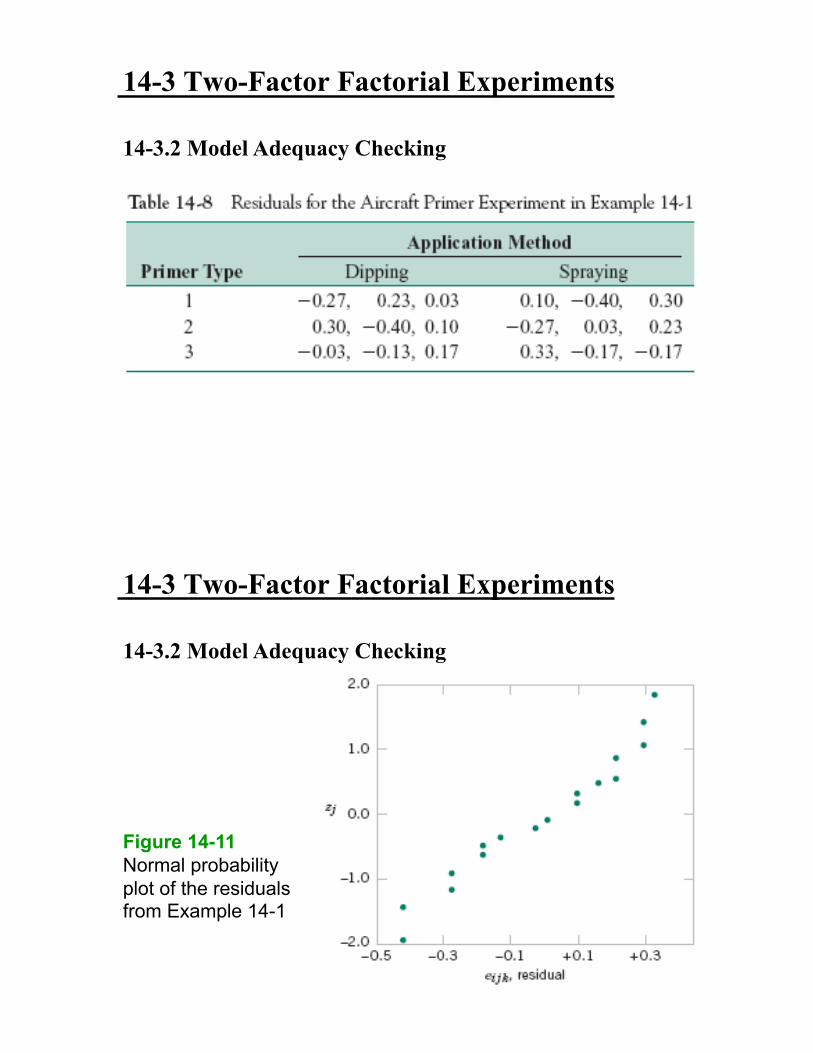
14-3 Two-Factor Factorial Experiments
14-3.2 Model Adequacy Checking
14-3 Two-Factor Factorial Experiments
14-3.2 Model Adequacy Checking
Figure 14-11
Normal probability
plot of the residuals from Example 14-1

14-3 Two-Factor Factorial Experiments
14-3.2 Model Adequacy Checking
Figure 14-14 Plot of residuals versus predicted values.
14-4 General Factorial Experiments
Model for a three-factor factorial experiment

14-4 General Factorial Experiments
Example 14-2

R commands and outputs Example 14-2: enter data by row
> Roughness=c(9,11,9,10, 7,10,11,8, 10,10,12,16, 12,13,15,14)
> Feed=c(1,1,1,1, 1,1,1,1, 2,2,2,2, 2,2,2,2)
> Depth=c(1,1,2,2, 1,1,2,2, 1,1,2,2, 1,1,2,2)
> Angle=c(1,2,1,2, 1,2,1,2, 1,2,1,2, 1,2,1,2)
> g=lm(Roughness ~ Feed*Depth*Angle)
> anova(g)
Response: Roughness
Df Sum Sq Mean Sq F value Pr(>F)
Feed 1 45.562 45.562 18.6923 0.002534 **
Depth 1 10.562 10.562 4.3333 0.070931 .
Angle 1 3.062 3.062 1.2564 0.294849
Feed:Depth 1 7.562 7.562 3.1026 0.116197
Feed:Angle 1 0.062 0.062 0.0256 0.876749
Depth:Angle 1 1.562 1.562 0.6410 0.446463
Feed:Depth:Angle 1 5.062 5.062 2.0769 0.187512
Residuals 8 19.500 2.438
> par(mfrow=c(1,3)) #
> interaction.plot(Feed, Depth, Roughness)
> interaction.plot(Feed, Angle, Roughness)
> interaction.plot(Angle, Depth, Roughness)
14-4 General Factorial Experiments
Example 14-2

Bootstrap Method
15-1 Introduction
•! Most of the hypothesis-testing and confidence
interval procedures discussed in previous chapters
are based on the assumption that we are working
with random samples from normal populations.
•! These procedures are often called parametric methods
•! In this chapter, nonparametric and distribution free
methods will be discussed.
•! We usually make no assumptions about the distribution
of the underlying population.

15-2 Sign Test
15-2.1 Description of the Test
•! The sign test is used to test hypotheses about the
median of a continuous distribution.
•!Let R+ represent the number of differences
that are positive.
•! What is the sampling distribution of R+ under H0?
0
~µ!iX
15-2 Sign Test
15-2.1 Description of the Test
If the following hypotheses are being tested:
The appropriate P-value is
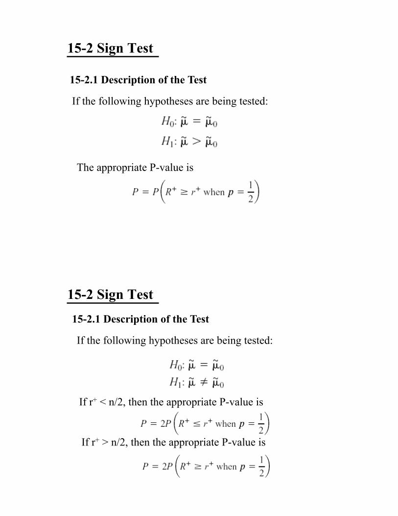
15-2 Sign Test
15-2.1 Description of the Test
If the following hypotheses are being tested:
The appropriate P-value is
15-2 Sign Test
15-2.1 Description of the Test
If the following hypotheses are being tested:
If r+ < n/2, then the appropriate P-value is
If r+ > n/2, then the appropriate P-value is
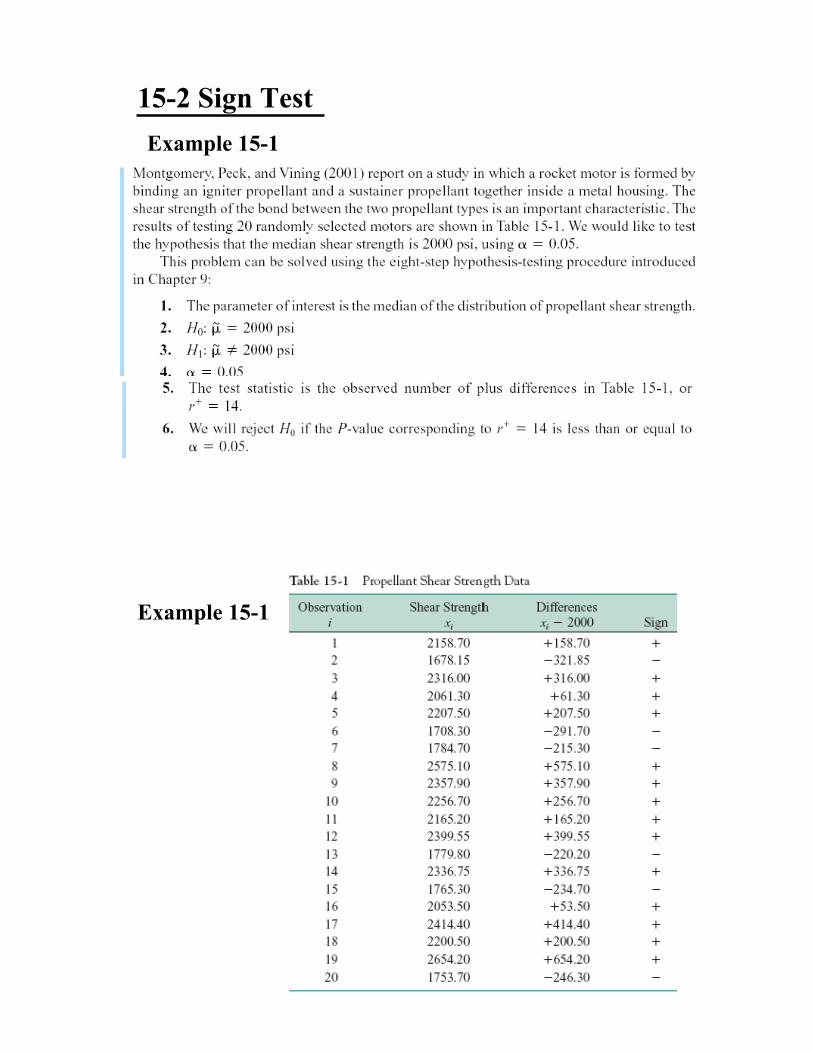
15-2 Sign Test
Example 15-1
Example 15-1
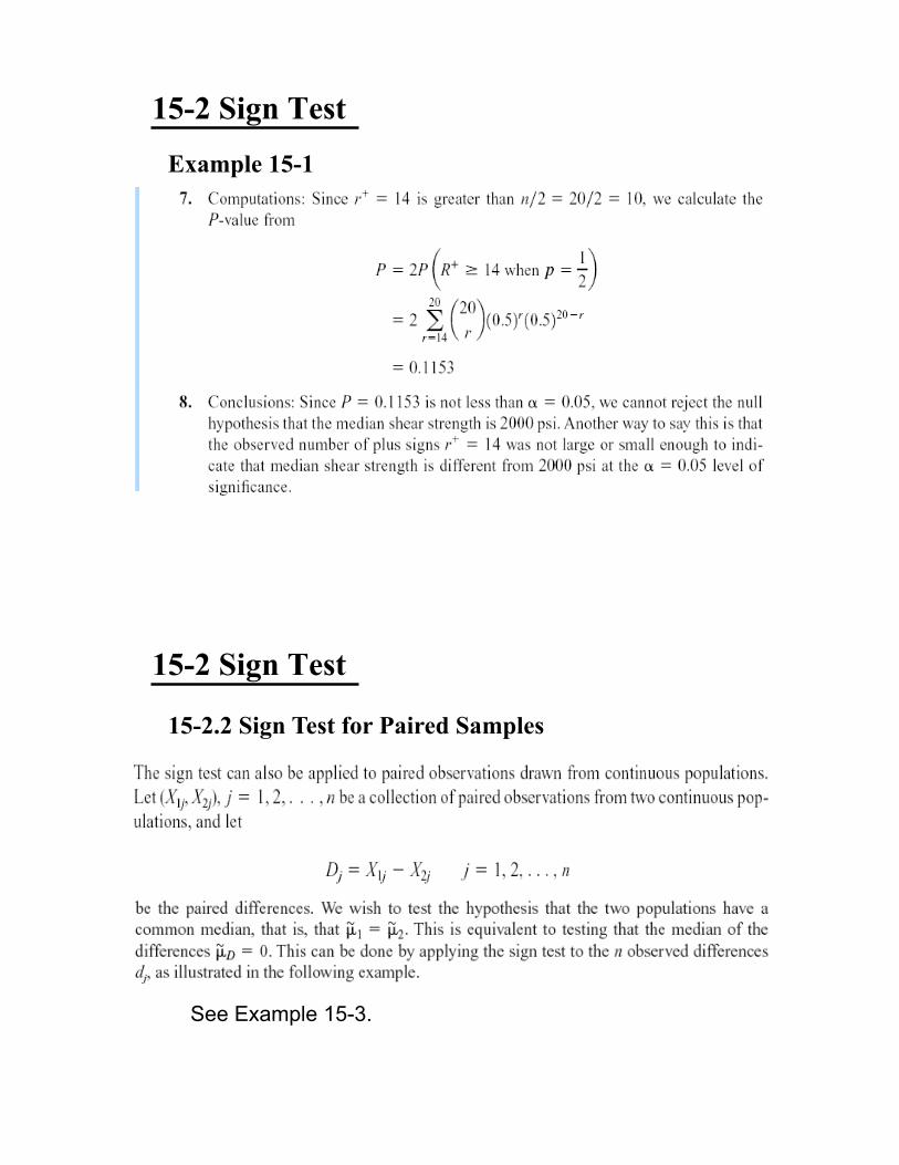
15-2 Sign Test
Example 15-1
15-2 Sign Test
15-2.2 Sign Test for Paired Samples
See Example 15-3.
15-2 Sign Test
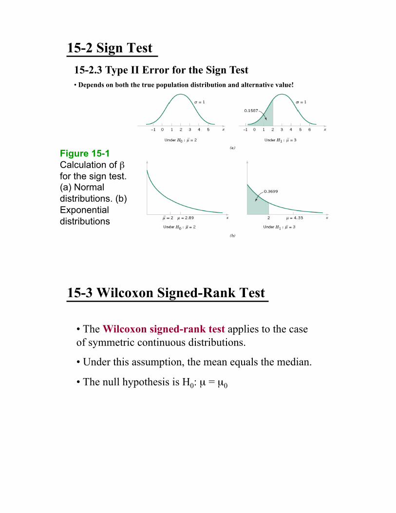
15-2.3 Type II Error for the Sign Test
•! Depends on both the true population distribution and alternative value!
Figure 15-1
Calculation of !
for the sign test. (a) Normal
distributions. (b)
Exponential
distributions
15-3 Wilcoxon Signed-Rank Test
•! The Wilcoxon signed-rank test applies to the case
of symmetric continuous distributions.
•! Under this assumption, the mean equals the median.
•! The null hypothesis is H0: µ = µ0

15-3 Wilcoxon Signed-Rank Test
•! Assume that X1, X2, …, Xn is a random sample from a continuous
and symmetric distribution with mean (and median) µ.
Procedure:
•! Compute the differences Xi ! µ0, i = 1, 2, …, n.
•! Rank the absolute differences |Xi ! µ0|, i = 1, 2, …, n in ascending
order.
•! Give the ranks the signs of their corresponding differences.
•! Let W+ be the sum of the positive ranks and W! be the absolute
value of the sum of the negative ranks.
•! Let W = min(W+, W!).
•! 15-3.1 Description of the Test
15-3 Wilcoxon Signed-Rank Test
Decision rules:

15-3 Wilcoxon Signed-Rank Test
Example 15-4
Example 15-4

15-3 Wilcoxon Signed-Rank Test
Example 15-4
15-3 Wilcoxon Signed-Rank Test
15-3.2 Large-Sample Approximation
Z0 is approximately standard normal when n is large.

15-4 Wilcoxon Rank-Sum Test
15-4.1 Description of the Test
15-4 Wilcoxon Rank-Sum Test
15-4.1 Description of the Test

15-4 Wilcoxon Rank-Sum Test
Example 15-6
15-4 Wilcoxon Rank-Sum Test
Example 15-6

Example 15-6
15-4 Wilcoxon Rank-Sum Test
Example 15-6

15-5 Nonparametric Methods in the
Analysis of Variance
The single-factor analysis of variance model for
comparing a population means is
The hypothesis of interest is
The Kruskal-Wallis test (w/o assumption of normality)
•! Basic idea: Use ranks instead of actual numbers
Parametric vs. Nonparametric Tests
•! When the normality assumption is correct, t-test or F-test is more powerful. –! Wilcoxon signed-rank or rank-sum test is approximately 95% as
efficient as the t-test in large samples.
•! On the other hand, regardless of the form of the distributions, nonparametric tests may be more powerful. –! Wilcoxon signed-rank or rank-sum test will always be at least 86%
as efficient.
•! The efficiency of the Wilcoxon test relative to the t-test is usually high if the underlying distribution has heavier tails than the normal –! because the behavior of the t-test is very dependent on the sample
mean, which is quite unstable in heavy-tailed distributions.