Introduction to Statistics 18.05 Spring 2014

T T T H H T H H H T H T H T H T H T H T H T T T H T T T T H H T T H H T H H T H T T H H H H T H T H T T T H T H H H H T T T T H H H T T T H H H H H H H H T T T H T H H T T T H H T H T H H H T T T H H

January 1, 2017 1 / 23

Three ‘phases’

Data Collection: Informal Investigation / Observational Study / Formal Experiment

Descriptive statistics

Inferential statistics (the focus in 18.05)

To consult a statistician after an experiment is finished is often merely to ask him to conduct a post-mortem examination. He can perhaps say what the experiment died of.

R.A. Fisher

January 1, 2017 2 / 23

Is it fair?

T T T H H T H H H T H T H T H T H T H T H T T T H T T T T H H T T H H T H H T H T T H H H H T H T H T T T H T H H H H T T T T H H H T T T H H H H H H H H T T T H T H H T T T H H T H T H H H T T T H H

January 1, 2017 3 / 23

Is it normal?

Does it have µ = 0? Is it normal? Is it standard normal?

x

Den

sity

−4 −2 0 2 4

0.00

0.10

0.20

Sample mean = 0.38; sample standard deviation = 1.59

January 1, 2017 4 / 23

What is a statistic?

Definition. A statistic is anything that can be computed from the collected data. That is, a statistic must be observable.

Point statistic: a single value computed from data, e.g sample average xn or sample standard deviation sn.

Interval or range statistics: an interval [a, b] computed from the data. (Just a pair of point statistics.) Often written as x ± s.

Important: A statistic is itself a random variable since a new experiment will produce new data to compute it.

January 1, 2017 5 / 23

Concept question

You believe that the lifetimes of a certain type of lightbulb follow an exponential distribution with parameter λ. To test this hypothesis you measure the lifetime of 5 bulbs and get data x1, . . . x5.

Which of the following are statistics? x1+x2+x3+x4+x5(a) The sample average x =

5 .

(b) The expected value of a sample, namely 1/λ.

(c) The difference between x and 1/λ.

1. (a) 2. (b) 3. (c) 4. (a) and (b) 5. (a) and (c) 6. (b) and (c) 7. all three 8. none of them

answer: 1. (a). λ is a parameter of the distribution it cannot be computed from the data. It can only be estimated.

January 1, 2017 6 / 23

Notation

Big letters X , Y , Xi are random variables.

Little letters x , y , xi are data (values) generated by the random variables.

Example. Experiment: 10 flips of a coin:

Xi is the random variable for the i th flip: either 0 or 1.

xi is the actual result (data) from the i th flip. e.g. x1, . . . , x10 = 1, 1, 1, 0, 0, 0, 0, 0, 1, 0.

January 1, 2017 7 / 23

Reminder of Bayes’ theorem

Bayes’s theorem is the key to our view of statistics. (Much more next week!)

P(D|H)P(H)P(H|D) = .

P(D)

P(data|hypothesis)P(hypothesis) P(hypothesis|data) =

P(data)

January 1, 2017 8 / 23

Estimating a parameter

Example. Suppose we want to know the percentage p of people for whom cilantro tastes like soap.

Experiment: Ask n random people to taste cilantro.

Model: Xi ∼ Bernoulli(p) is whether the i th person says it tastes like soap.

Data: x1, . . . , xn are the results of the experiment

Inference: Estimate p from the data.

January 1, 2017 9 / 23

Parameters of interest

Example. You ask 100 people to taste cilantro and 55 say it tastes like soap. Use this data to estimate p the fraction of all people for whom it tastes like soap.

So, p is the parameter of interest.

January 1, 2017 10 / 23

Likelihood

For a given value of p the probability of getting 55 ‘successes’ is the binomial probability

100 P(55 soap|p) = p 55(1 − p)45 .

55

Definition: 100

The likelihood P(data|p) = p 55(1 − p)45 . 55

NOTICE: The likelihood takes the data as fixed and computes the probability of the data for a given p.

January 1, 2017 11 / 23

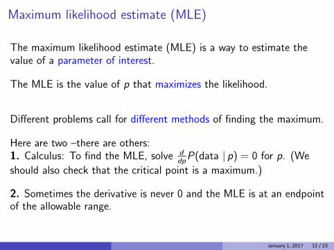
Maximum likelihood estimate (MLE)

The maximum likelihood estimate (MLE) is a way to estimate the value of a parameter of interest.

The MLE is the value of p that maximizes the likelihood.

Different problems call for different methods of finding the maximum.

Here are two –there are others: 1. Calculus: To find the MLE, solve d P(data | p) = 0 for p. (We

dp

should also check that the critical point is a maximum.)

2. Sometimes the derivative is never 0 and the MLE is at an endpoint of the allowable range.

January 1, 2017 12 / 23

Cilantro tasting MLE

The MLE for the cilantro tasting experiment is found by calculus.

dP(data | p) 100 = (55p 54(1 − p)45 − 45p 55(1 − p)44) = 0

dp 55

A sequence of algebraic steps gives:

55(1 − p)4455p 54(1 − p)45 = 45p

55(1 − p) = 45p

55 = 100p

Therefore the MLE is p̂ = 55 100 .

January 1, 2017 13 / 23

( )

Log likelihood

Because the log function turns multiplication into addition it is often convenient to use the log of the likelihood function

log likelihood = ln(likelihood) = ln(P(data | p)).

Example.

100 Likelihood P(data|p) = p 55(1 − p)45

55

100 Log likelihood = ln + 55 ln(p) + 45 ln(1 − p).

55

(Note first term is just a constant.)

January 1, 2017 14 / 23

(( ))( )

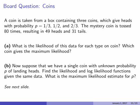
Board Question: Coins

A coin is taken from a box containing three coins, which give heads with probability p = 1/3, 1/2, and 2/3. The mystery coin is tossed 80 times, resulting in 49 heads and 31 tails.

(a) What is the likelihood of this data for each type on coin? Which coin gives the maximum likelihood?

(b) Now suppose that we have a single coin with unknown probability p of landing heads. Find the likelihood and log likelihood functions given the same data. What is the maximum likelihood estimate for p?

See next slide.

January 1, 2017 15 / 23

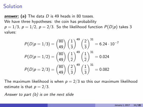
Solution

answer: (a) The data D is 49 heads in 80 tosses. We have three hypotheses: the coin has probability p = 1/3, p = 1/2, p = 2/3. So the likelihood function P(D|p) takes 3 values:

49 3180 1 2 P(D|p = 1/3) = = 6.24 · 10−7

49 3 3 49 3180 1 1

P(D|p = 1/2) = = 0.024 49 2 2

49 3180 2 1 P(D|p = 2/3) = = 0.082

49 3 3

The maximum likelihood is when p = 2/3 so this our maximum likelihood estimate is that p = 2/3.

Answer to part (b) is on the next slide

January 1, 2017 16 / 23

( )( ) ( )( )( ) ( )( )( ) ( )

/ 22

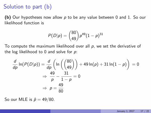
Solution to part (b)

(b) Our hypotheses now allow p to be any value between 0 and 1. So our likelihood function is

80 P(D|p) = p 49(1 − p)31

49

To compute the maximum likelihood over all p, we set the derivative of the log likelihood to 0 and solve for p:

d d 80 ln(P(D|p)) = ln + 49 ln(p) + 31 ln(1 − p) = 0

dp dp 49 49 31 ⇒ − = 0 p 1 − p

49 ⇒ p = 80

So our MLE is p̂ = 49/80.

January 1, 2017 17 / 23

( )

( (( )) )

January 1, 2017 17 / 22

Continuous likelihood

Use the pdf instead of the pmf

Example. Light bulbs

Lifetime of each bulb ∼ exp(λ).

Test 5 bulbs and find lifetimes of x1, . . . , x5.

(i) Find the likelihood and log likelihood functions. (ii) Then find the maximum likelihood estimate (MLE) for λ.

answer: See next slide.

January 1, 2017 18 / 23

�

Solution

(i) Let Xi ∼ exp(λ) = the lifetime of the i th bulb.

Likelihood = joint pdf (assuming independence):

−λ(x1+x2+x3+x4+x5)f (x1, x2, x3, x4, x5|λ) = λ5 e .

Log likelihood

ln(f (x1, x2, x3, x4, x5|λ)) = 5 ln(λ) − λ(x1 + x2 + x3 + x4 + x5).

(ii) Using calculus to find the MLE:

d ln(f (x1, x2, x3, x4, x5|λ)) 5 5ˆ= − xi = 0 ⇒ λ = � . d λ λ xi

January 1, 2017 19 / 23

Board Question

Suppose the 5 bulbs are tested and have lifetimes of 2, 3, 1, 3, 4 years respectively. What is the maximum likelihood estimate (MLE) for λ?

Work from scratch. Do not simply use the formula just given.

Set the problem up carefully by defining random variables and densities.

Solution on next slide.

January 1, 2017 20 / 23

Solution

answer: We need to be careful with our notation. With five different values it is best to use subscripts. So, let Xj be the lifetime of the i th bulb

−λxiand let xi be the value it takes. Then Xi has density λe . We assume each of the lifetimes is independent, so we get a joint density

−λ(x1+x2+x3+x4+x5)f (x1, x2, x3, x4, x5|λ) = λ5 e .

Note, we write this as a conditional density, since it depends on λ. This density is our likelihood function. Our data had values

x1 = 2, x2 = 3, x3 = 1, x4 = 3, x5 = 4.

So our likelihood and log likelihood functions with this data are

−13λf (2, 3, 1, 3, 4 | λ) = λ5 e , ln(f (2, 3, 1, 3, 4 | λ)) = 5 ln(λ) − 13λ

Continued on next slide

January 1, 2017 21 / 23

Solution continued

Using calculus to find the MLE we take the derivative of the log likelihood

5 − 13 = 0 ⇒ λ̂ = 5

. λ 13

January 1, 2017 22 / 23

MIT OpenCourseWarehttps://ocw.mit.edu

18.05 Introduction to Probability and StatisticsSpring 2014

For information about citing these materials or our Terms of Use, visit: https://ocw.mit.edu/terms.