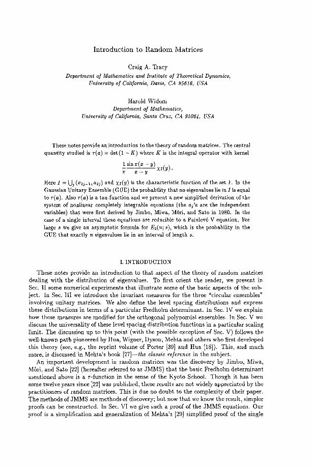
Introduction to Random Matrices

Craig A. Tracy

Department of Mathematics and Institute of Theoretical Dynamics, University of California, Davis, CA 95616, USA

Harold Widom Department of Mathematics,

University of California, Santa Cruz, CA 95064, USA

These notes provide an introduction to the theory of random matrices. The central quantity studied is r(a) = det (1 - K) where K is the integral operator with kernel

1 sin r (z - y) XI(Y). 7r x - y

Here I = [-Ji (a2j-l,a2J) and XI(Y) is the characteristic function of the set I . In the Gaussian Unitary Ensemble (GUE) the probability that no eigenvalues lie in I is equal to v(a). Also v(a) is a tau-function and we present a new simplified derivation of the system of nonlinear completely integrable equations (the aj's a r e the independent variables) that were first derived by Jimbo, Miwa, M6ri, and Sato in 1980. In the case of a single interval these equations are reducible to a Painlev~ V equation. For large s we give an asymptotic formula for E2(n; s), which is the probability in the GUE that exactly n eigenvalues lie in an interval of length s.

I. INTRODUCTION

These notes provide an introduction to that aspect of the theory of random matrices dealing with the distribution of eigenvalues. To first orient the reader, we present in Sec. II some numerical experiments that illustrate some of the basic aspects of the sub- ject. In Sec. III we introduce the invariant measures for the three "circular ensembles" involving unitary matrices. We also define the level spacing distributions and express these distributions in terms of a particular Fredholm determinant. In Sec. IV we explain how these measures are modified for the orthogonal polynomial ensembles. In Sec. V we discuss the universality of these level spacing distribution functions in a particular scaling limit. The discussion up to this point (with the possible exception of Sec. V) follows the well-known path pioneered by Hua, Wigner, Dyson, Mehta and others who first developed this theory (see, e.g., the reprint volume of Porter [39] and Hua [18]). This, and much more, is discussed in Mehta's book [27f--the classic reference in the subject.

An important development in random matrices was the discovery by Jimbo, Miwa, M6ri, and Sato [22] (hereafter referred to as JMMS) that the basic Fredholm determinant mentioned above is a r-function in the sense of the Kyoto School. Though it has been some twelve years since [22] was published, these results are not widely appreciated by the practitioners of random matrices. This is due no doubt to the complexity of their paper. The methods of JMMS are methods of discovery; but now that we know the result, simpler proofs can be constructed. In Sec. VI we give such a proof of the JMMS equations. Our proof is a simplification and generalization of Mehta's [29] simplified proof of the single

104

interval case. Also our methods build on the earlier work of Its, Izergin, Korepin, and Slavnov [19] and Dyson [13]. We include in this section a discussion of the connection between the JMMS equations and the integrable Hamiltonian systems that appear in the geometry of quadrics and spectral theory as developed by Moser [35]. This section concludes with a discussion of the case of a single interval (viz., probability that exactly n eigenvalues lie in a given interval). In this case the JMMS equations can be reduced to a single ordinary differential equat ion-- the Painlev4 V equation.

Finally, in Sec. VII we discuss the asymptotics in the case of a large single interval of the various level spacing distribution functions [4, 43, 31]. In this analysis both the Painlev4 representation and new results in Toeplitz/Wiener-Hopf theory are needed to produce these asymptotics. We also give an approach based on the asymptotics of the eigenvalues of the basic linear integral operator [15, 27, 40]. These results are then compared with the continuum model calculations of Dyson [13].

II. NUMERICAL EXPERIMENTS

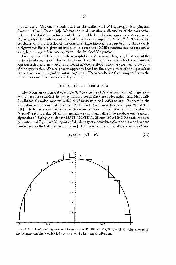
The Gaussian orthogonal ensemble (GOE) consists of N x N real symmetric matrices whose elements (subject to the symmetric constraint) are independent and identically distributed Gaussian random variables of mean zero and variance one. Pioneers in the simulation of random matrices were Porter and Rosenzweig (see, e.g., pgs. 235-299 in [39]). Today one can easily use a Gaussian random number generator to produce a "typical" such matrix. Given this matrix we can diagonalize it to produce our "random eigenvalues." Using the software MATHEMATICA, 25 such 100 x 100 GOE matrices were generated and Fig. 1 is a histogram of the density of eigenvalues where the x-axis has been normalized so that all eigenvalues lie in [ -1 , 1]. Also shown is the Wigner semicircle law

p w ( x ) = "~x/'l - x 2. (2.1) T"

0.7

0.6

0.5

0.4

0.3

0.2

0.i

-i -0.5 0.5 1

FIG. 1. Density of eigenvalues histogram for 25, 100 x 100 GOE matrices. Also plotted is the Wigner semicircle which is known to be the limiting distribution.

0.2

0.5

0.4

Density

-i

0.i

-0.5 0.5 1

105

FIG. 2. Density of eigenvalues histogram for 25, 100 x 100 symmetric matrices whose ele- ments are uniformly distributed on [-1,1]. Also plotted is the Wigner semicircle distribution.

Given any such. distribution (or density) function, one can ask to what extent is it "universal." In Fig. 2 we plot the same density histogram except we change the distri- bution of matrix elements to the uniform distribution on [ -1 , 1]. One sees that the same semicircle law is a good approximation to the density of eigenvalues. See [27] for further discussion of the Wigner semicircle law.

A fundamental quantity of the theory is the (conditional) probability that given an eigenvalue at a, the next eigenvalue lies between b and b+db: p(0; a, b) db. In measuring this quantity it is usually assumed that the system is well approximated by a translationally invariant system of constant eigenvalue density. This density is conveniently normalized to one. In the translationally invariant system p(0; a, b) will depend only upon the difference s := b - a. When there is no chance for confusion, we denote this probability density simply by p(s). Now as Figs. 1 and 2 clearly show, the eigenvalue density in the above examples is not constant. However, since we are mainly interested in the case of large matrices (and ultimately N --+ c¢), we take for our data the eigenvalues lying in an interval in which the density does not change significantly. For this data we compute a histogram of spacings of eigenvalues. That is to say, we order the eigenvalues Ei and compute the level spacings Si := Ei+1 - Ei. The scale of both the x-axis and y-axis are fixed once we require that the integrated density is one and the mean spacing is one. Fig. 3 shows the resulting histogram for 20, 100 x 100 GOE matrices where the eigenvalues were taken from the middle half of the entire eigenvalue spectrum. The important aspect of this data is it shows level repulsion of eigenvalues as indicated by the vanishing of p(s) for small s. Also plotted is the Wignev surmise

pw(s) = ~sexp -- s 2 (2.2)

p(s)

o.8

p(s)

0.6

0.4

0.2

i ! s

1 2 3 4

FIG. 3, Level spacing histogram for 20~ 100 × 100 GOE matrices. Also plotted is the Wigner surmise (2.2).

0.7

0.6

0.5

0.4

0.3

0.2

0.i

, , , i , , , , , , ,

1 2

106

3 '

FIG. 4. Level spacing histogram for 50, 100 × 100 symmetric matrices whose elements are uniformly distributed on [-1, 1]. Also plotted is the Wigner surmise (2.2).

which for these purposes numerically well approximates the exact result (to be discussed below) in the range 0 < s < 3. In Fig. 4 we show the same histogram except now the data are from 50, 100 x 100 real symmetric matrices whose elements are iid random variables with uniform distribution on [-1, 1]. In computing these histograms, the spacings were computed for each realization of a random matrix, and then the level spacings of several experiments were lumped together to form the data. If one first forms the data by mixing

p(s)

1

0 . 8

0 . 6

0 . 4

0 . 2

107

, i i , i i i , , i , i i i / i , J , i ,

1 2 3 4

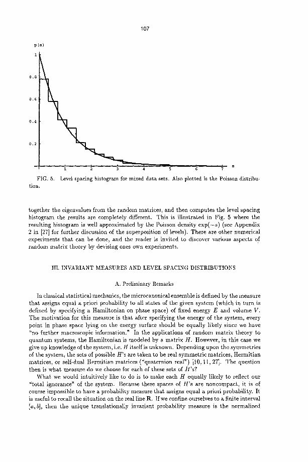
FIG. 5. tion.

' 5 '~ ' ' ~

Level spacing histogram for mixed data sets. Also plotted is the Poisson distribu-

-together the eigenvalues from the random matrices, and then computes the level spacing histogram the results are completely different. This is illustrated in Fig. 5 where the resulting histogram is well approximated by the Poisson density e x p ( - s ) (see Appendix 2 in [27] for further discussion of the superposition of levels). There are other numerical experiments that can be done, and the reader is invited to discover various aspects of random matrix theory by devising ones own experiments.

III. INVARIANT MEASUI~ES AND LEVEL SPACING DISTRIBUTIONS

A. Preliminary Remarks

In classical statistical mechanics, the microcanonical ensemble is defined by the measure that assigns equal a priori probability to all states of the given system (which in turn is defined by specifying a Hamiltonian on phase space) of fixed energy E and volume V. The motivation for this measure is that after specifying the energy of the system, every point in phase space lying on the energy surface should be equally likely since we have "no further macroscopic information." In the applications of random matrix theory to quantum systems, the Hamiltonian is modeled by a matrix H. However, in this case we give up knowledge of the system, i.e. H itself is unknown. Depending upon the symmetries of the system, the sets of possible H's are taken to be real symmetric matrices, Hermitian matrices, or self-dual Hermitian matrices ("quaternion real") [10, 11, 27]. The question then is what measure do we choose for each of these sets of H's?

What we would intuitively like to do is to make each H equally likely to reflect our "total ignorance" of the system. Because these spaces of H 's are noncompact, it is of course impossible to have a probability measure that assigns equal a priori probability. It is useful to recall the situation on the real line R. If we confine ourselves to a finite interval [a, b], then the unique translationally invariant probability measure is the normalized

108

Lebesgue measure. Another characterization of this probability measure is that it is the unique density that maximizes the information entropy

Sip] = - f ~ p(x)log p(x) dx. (3.1)

On R the maximum entropy density subject to the constraints E(1) = 1 and E(x 2) = a 2 is the Gaussian density of variance a 2. The Gaussian ensembles of random matrix theory can also be characterized as those measures that have maximum information entropy subject to the constraint of a fixed value of E(H*H) [1, 41]. The well-known explicit formulas are given below in Sec. IV.

Another approach, first taken by Dyson [10] and the one we follow here, is to consider unitary matrices rather than hermitian matrices. The advantage here is that the space of unitary matrices is compact and the eigenvalue density is constant (translationally invariant distributions).

B. Haar Measure for U(N)

We denote by G = U(N) the set of N × N unitary matrices and recall that d imRU(N ) = N 2. One can think of U(N) as an N2-dimensional submanifold of R 2N2

under the identification of a complex N × N matrix with a point in R 2N2. The group G acts on itself by either left or right translations, i.e. fix go C G then

Lgo : g--* gog and Rgo : g--* ggo.

The normalized Haar measure it2 is the unique probability measure on G that is both left- and right-invariant:

,u2(gE) = #2(Eg) = p2(E) (3.2)

for all g E G and every measurable set E (the reason for the subscript 2 will become clear below). Since for compact groups a measure that is left-invariant is also right-invariant, we need only construct a left-invariant measure to obtain the Haar measure. The invariance (3.2) reflects the precise meaning of "total ignorance" and is the analogue of translational invariance picking out the Lebesgue measure.

To construct the Haar measure we construct the matrix of left-invariant 1-forms

f~a =g-ldg, g C G, (3.3)

where ~g is anti-Hermitian since g is unitary. Choosing N 2 linearly independent 1-forms wlj from ~g, we form the associated volume form obtained by taking the wedge product of these wlj's. This volume form on G is left-invariant, and hence up to normalization, it is the desired probability measure.

Another way to contruct the Haar measure is to introduce the standard Riemannian metric on the space of N × N complex matrices Z = (zq):

N

(ds) 2 = tr(dZdZ') = ~ Idz,jl ~. j,k= l

We now restrict this metric to the submanifold of unitary matrices. A simple computation shows the restricted metric is

(ds) 2 = tr (ftgf~;). (3.4)

109

Since f~9 is left-invariant, so is the metric (ds) 2. If we use the standard Riemannian formulas to construct the volume element, we will arrive at the invariant volume form.

We are interested in the induced probability density on the eigenvalues. This calcu- lation is classical and can be found in [18, 42]. The derivation is particularly clear if we make use of the Riemannian metric (3.4). To this end we write

g = X O X -1 , g e G , (3.5)

where X is a unitary matrix and D is a diagonal matrix whose diagonal elements we write as exp(i~k). Up to an ordering of the angles c2k the matrix D is unique. We can assume that the eigenvalues are distinct since the degenerate case has measure zero. Thus X is determined up to a diagonal unitary matrix. If we denote by T(N) the subgroup of diagonal unitary matrices, then to each 9 E G there corresponds a unique pair (X, D), 2( E G/T(N) and D e T(N). The Haar measure induces a measure on G/T(N) (via the natural projection map). Since

we have

X*dgX = f x D - D~x + dD,

(ds) 2 = tr ( f ig f ; ) = tr (dg dg*) = tr (X*dgXX*dg*X)

= tr ([fix, D] [fix, D]*) + tr (dD dD*) N N

= ~ 16xk, (exp( iW) - e x p ( / ~ ) ) l ~ + ~ ( d ~ ) ~ k,g=l k=l

where f x = (6Xke). Note that the diagonal elements/~Xkk do not appear in the metric. Using the Riemannian volume formula we obtain the volume form

0)g • CO X H lexp(ictPJ) -- exp(i~r~k)l 2 d¥~l "" ' d ~ N (3 ,6) j<k

where wx = const l-]j>~ ~Xj~. We now integrate over the entire group G subject to the condition that the elements

have their angles between ~k and ~ + d~k to obtain

T h e o r e m 1 The volume of that part of the unitary group U(N) whose elements have their angles between ~k and ~k + d~ok is given by

PN2(~01,..., ~N) d~l"" dcpN = CN2 H [exp(i~j) -- exp(icpk)]2 dCpl " " • d~N (3.7) j<k

where CN2 is a normalization constant.

We mention that there exist algorithms [8] to generate unitary matrices that are Haar distributed. The algorithm of Diaconis and Shahshahani [8] is of order N 3 and is easily implemented on a computer.

C. Orthogonal and Symplectic Ensembles

Dyson [11], in a careful analysis of the implications of time-reversM invariance for phys- ical systems, showed that (a) systems having time-reversal invariance and rotational sym- metry or having time-reversal invariance and integral spin are characterized by symmetric unitary matrices; and (b) those systems having time-reversal invariance and half-integral spin but no rotational symmetry are characterized by self-duM unitary matrices (see also

110

Chp. 9 in [27]). For systems without time-reversal invariance there is no restriction on the unitary matrices. These three sets of unitary matrices along with their respective invariant measures, which we denote by E~(N), fl -- 1,4, 2, respectively, constitute the circular ensembles. We denote the invariant measures by #~, e.g. #2 is the normalized Haar measure discussed in Sec. III B.

A symmetric unitary matrix S can be written as

s = vTv, V C U(N).

Such a decomposition is not unique since

V--*RV, R E O ( N ) ,

leaves S unchanged. Thus the space of symmetric unitary matrices can be identified with the coset space

U(N)/O(N).

The group G = U(N) acts on the coset space U(N)/O(N), and we want the invariant measure #1. If 7: denotes the natural projection map G ~ G/H, then the measure #1 is just the induced measure:

~I(B) = ~2(~-1(B)),

and hence Ea(N) can be identified with the pair (U(N)/O(N), #~). The space of self-dual unitary matrices can be identified (for even N) with the coset

space

U(N)/Sp(N/2)

where Sp(N) is the symplectic group. Similarly, the circular ensemble E4(N) can be identified with (U(N)/Sp(N/2), #4) where/~4 is the induced measure.

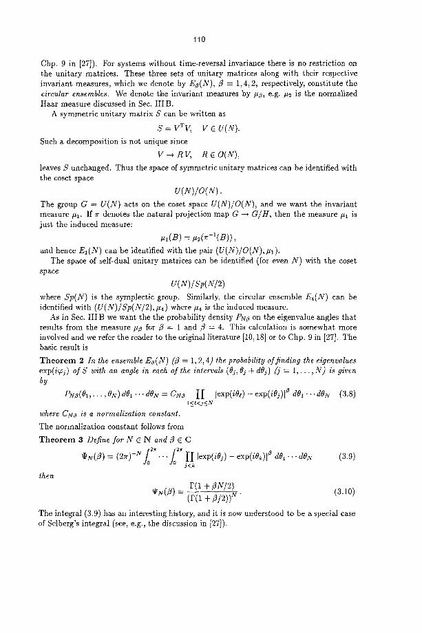
As in Sec. III B we want the the probability density PNO on the eigenvMue angles that results from the measure #3 for fl = 1 and fl = 4. This calculation is somewhat more involved and we refer the reader to the original literature [10, 18] or to Chp. 9 in [27]. The basic result is

T h e o r e m 2 In the ensemble E~(N) (fl = 1,2, 4) the probability of finding the eigenvalues exp(iwj) ors with an angle in each of the intervals (~j, Oj + dOj) (j = 1,. . . ,N) is given by

PN3(O1,...,ON)dOI'''dON = CN~ 1-I lexp(iO,)-exp(iOj)l~ dO1...dON (3.8) l<g<j<N

where CNfl is a normalization constant.

The normalization constant follows from

T h e o r e m 3 Define for N C N and fl C C

~N(fl) = (2~r) -~v f02~ ' ' ' fo ~ l ' I lexp(iOj) -- exp(iOk)l ~ dOa.., dON (3.9) j<k

then tpg(3) _ F(1 + 3N/2)

(F(1 + fl/2)) N (3.10)

The integral (3.9) has an interesting history, and it is now understood to be a special case of Selberg's integral (see, e.g., the discussion in [27]).

111

D. Physical Interpretation of the Probability Density PNZ

The 2D Coulomb potential for N unit like charges on a circle of radius one is

WN( 01'''" 'ON) = -- E log [exp(i0j) - exp(iOk)[ , (3.11) l<_j<k<_N

Thus the (positional) equilibrium Gibbs measure at inverse temperature 0 </3 < c~ for this system of N charges with energy WN is

exp (--/3WN( Oi, . . . , ON)) (3.12) ~N(/3)

For the special cases of/3 = 1, 2, 4 this Gibbs measure is the probability density of The- orem 2. Thus in this mathematically equivalent description, the term "level repulsion" takes on the physical meaning of repulsion of charges. This Coulomb gas description is due to Dyson [10], and it suggests various physically natural approximations that would not otherwise be so clear.

E. Level Spacing Distribution Functions

For large matrices there is too much information in the probability densities PNz(O:, . . . ,ON) to be useful in comparison with data. Thus we want to integrate out some of this information. Since the probability density PN~(O:,. . . ,ON) is a completely symmetric function of its arguments, it is natural to introduce the n-point correlation functions

N! 2. 2. R , ~ ( O , , . . . , O , , ) - (3 fSn) ! foo " " f o PN,(O:, . . . ,ON)dO,~+:' ' 'dON. (3.13)

The case/3 = 2 is significantly simpler to handle and we limit our discussion here to this c a s e .

L e m m a 1

where

' ( ) PIv2(O1,...,ON) = ~.T det KN(Oj,Ok j,k=l

i s in(N(0j - Ok)/2) I<N(Oj' Ok) ~--- 27I" sin ((0j - 0k)/2)

(3.14)

(3.15)

Proof: Recalling the Vandermonde determinant we can write

YI ]exp(iOj) - exp(i0k)] 2 = de t (M T) det(M) (3.16) j < k

where M~k = exp (i(j - 1)0k). A simple calculation shows

(M~-~)s ~ = 2~D~si~(Oj, O~)L)~ (3.17)

where D is the diagonal matrix with entries exp ( i (N - 1)0j2) . Except for the normaliza- tion constant the lemma now follows. Getting the correct normalization constant requires a little more work (see, e.g., Chp. 5 in [27]). •

112

From this lemma and the combinatoric Theorem 5.2.1 of [27] follows

T h e o r e m 4 Let t~2(01,..., On) be the n-point function defined by (3.13)for the circular ensemble E2(N); then

• ( )1 ° ) P~2(01,.. ,On) = det KN(Oj,Ok j.k=l

where KN(Oj, Ok) is given by (3.1@

We now discuss the behavior for large N. The l-point correlation function

R~'2(01) = N (3.19) ' 2/r

is just the density, p, of eigenvalues with mean spacing D = lip. As the size of the matrices goes to infinity so does the density. Thus if we are to construct a meaningful limit as N --, co we must scale the angles Oj. This motivates the definition of the scaling limit

p ~ o o , Oj-~O, such that x j : = p 0 j E R is fixed. (3.20)

We will abbreviate this scaling limit by simply writing N ~ oe. In this limit

R~2(x~,... xn)dxl. . .dx~ := lim R~(O1,...,O~)dO~...dO~ (3.21) ' N ~ o o

where we used the slightly confusing notation of denoting the scaling limit of the n-point functions by the same symbol. From Theorem 4 follows

T h e o r e m 5 In the scaling limit (3.20) the n-point functions become

n R~2(zl,...,z~)=det(h'(zi, xk)lj,k=l) (3.22)

where the kernel K(x, y) is given by

K(x, y) - 1 sin ~r(x - y) (3.23) 7r x - y

The three sets of correlation functions

CZ := {R~z(xl, . . . ,xn);xj e R}~°°_,, /3 = 1,2,4, (3.24)

define three different statistics (called the orthogonal ensemble, unitary ensemble, sym- plectic ensemble, respectively) of an infinite sequence of eigenvalues (or as we sometimes say, levels) on the real line.

We now have the necessary machinary to discuss the level spacing correlation functions in the ensemble C2. We denote by Z the union of m disjoint sub-intervals of the unit circle:

.2. = .2.1 U " * U -~"rn. (3 .25)

We begin with the probability of finding exactly nl eigenvalues in interval 2"1,..., nm eigenvalues in interval Zm in the ensemble E2(N). We denote this probability by E2N(nl,... ,nm;2") and we will let N --* ev at the end.

If XA denotes the characteristic function of the set A and n := nl + ' " + nm, then the probability we want is

113

., dOl'." dON PN2(01 . . . ON) n l . . . n m N - n '

n l n l +n2 n l + ' " + ~ m

× IIx~,(os,) II x~(o~#... II x~..(os~) Jl =1 3"2 =n l +1 jm=n , +.**+1

N

x 1"I ( 1 - x z ( O j ) ) . j = n + l

We define the quantities

r~,. . . . . = fo2~ d01 " " " fo2~ dO~ R~2( Oa , . . . , 0~ )

(3.26)

where

D(I;A)=det(1-~AjK(x'y)xIJ(Y)) ' j = l K ( z , y ) is given by (~.2~), ~nd n := n, + " " + n~.

(3.30)

nl nl +n2 n l + ' " + r i m

× II x~,(os,) Yi x~(oj2)... H ~(0~m). (3.27) j , =1 j 2 = n l +1 j m = n l + . . .+1

The idea is to expand the last product term in (3.26) involving the characteristic function X~ and to regroup the terms according to the number of times a factor of X~ appears. Doing this one can then integrate out those Ok variables that do not appear as arguments of any of the characteristic functions and express the result in terms of the quantities r , 2 ..... . To recognize the resulting terms we define the Fredholm determinant

Dg(g; A) = det 1 - A~KN(O, O')xz, (0'

where "~j~--1 AjKN(O, O')Xz,(O')" means the operator with that kernel and A is the m-tuple (A1,... , Am). A slight rewriting of the Fredholm expansion gives

M ~ . • • M " DN(Z; A) = 1 + E ( - 1 ) j E r.~. . . . . .

j=~ ,~>o j l ! ' - ' j r , ! J1 +- "+3m=3

The expansion above is then recognized to be proportional to

O"DN(Z; A) [ D

The scaling limit N ~ ~ can be taken with the result:

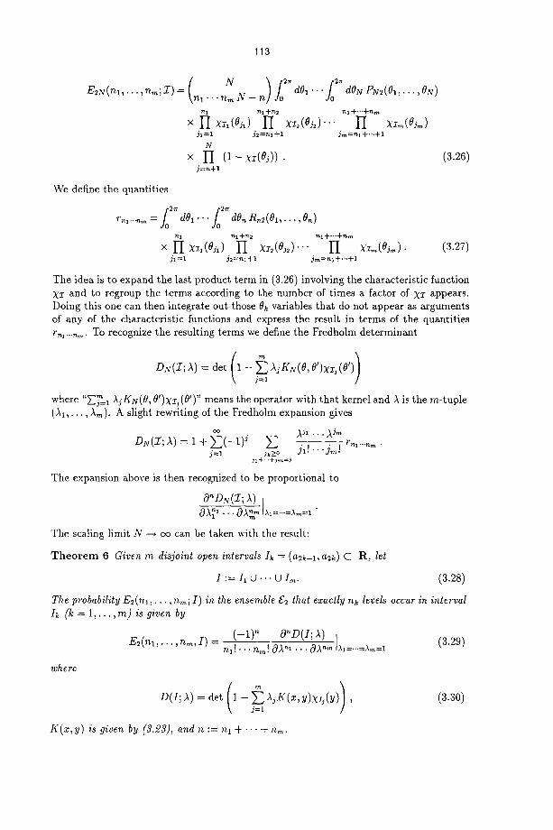
T h e o r e m 6 Given m disjoint open intervals Ik = ( a ~ - l , a2k) C R , let

I :=/1 U. . - U I,~. (3.28)

The probability E2(nl , . . . , nm; I) in the ensemble ~2 that exactly nk levels occur in interval I~ (k = 1 , . . . , m ) is given by

E~(~ .. n ~ , / ) = (_-))L ~D:I;~ (3.2o) ' "' n l ! ' . ' n , J O A ~ . . . O A ~ A . . . . . . Am=~

114

In the case of a single interval I = (a, b), we write the probability in ensemble £'Z of exactly n eigenvalues in I as Ez(n; s) where s := b - a. Mehta [27, 28] has shown that if we define

D+(s; A) = det (1 - AK+) (3.31)

where K± are the operators with kernels K(x, y) 5= K ( - x , y), and

E±(n; s) - ( -1)~ O'~D±(s; A) I (3.32)

then E,(0; s) = E+(0; a),

E+(~;~) = < ( 2 n ; , ) + E l ( 2 n - 1;.~), ~ > 0 , (a.33)

E_(n;s) = El(2n;s) + El(2n + 1;s), n > 0 , (3.34)

and

E4(n;s) = 2(E+(n;2s)+ E_(n;2s)) , n _> 0. (3.35)

Using the Fredholm expansion, small s expansions can be found for Ez(n; s). We quote [27, 28] here only the results for n = 0:

~2S3 T:4S 5

E l ( 0 ; s ) = l - s + 36- 120~ + O ( s 6 ) ' 7r28 4 71-4q 6

E~(0;~)= 1 - ~ + 3~- 675 ~ O ( s g , 87/'486

/{?4(0; s) = 1 - s + ~ + O(sS). (3.36)

The conditional probability in the ensemble SZ of an eigenvalue between b and b+ db given an eigenvalue at a, is given [27] by pz(0; s) ds where

d~E~(o; s) (3.37) pz(0; s) -- ds 2

Using this formula and the expansions (3.36) we see that pz(0; s) = O(sZ), making con- nection with the numerical results discussed in Sec. II. Note that the Wigner surmise (2.2) gives for small a the correct power of s for pl(0; s), but the slope is incorrect.

IV. ORTHOGONAL POLYNOMIAL ENSEMBLES

Orthogonal polynomial ensembles have been studied since the 1960's, e.g. [14], but recently interest has revived because of their application to the matrix models of 2D quantum gravity [7, 9, 16, 17]. Here we give the main results that generalize the previous sections.

The orthogonal polynomial ensemble associated to V assigns a probability measure on the space of N × N hermitian matrices proportional to

exp ( - T r (V(M))) dM (4.1)

where V(x) is a real-valued function such that

~(~) = exp (-V(x))

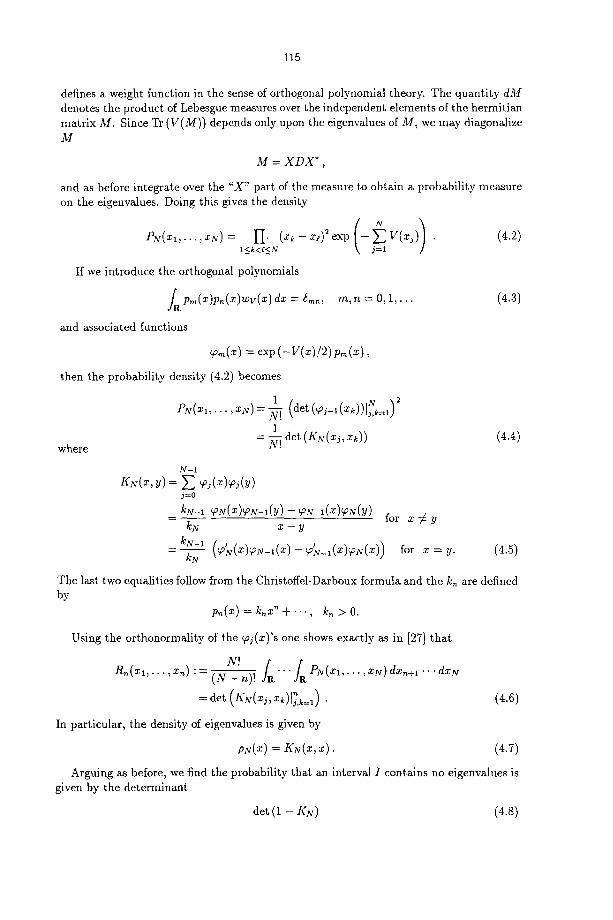
115

defines a weight function in the sense of orthogonal polynomial theory. The quantity dM denotes the product of Lebesgue measures over the independent elements of the hermitian matrix M. Since Tr (V(M)) depends only upon the eigenvalues of M, we may diagonalize M

where

M = X D X ' ,

and as before integrate over the "X" part of the measure to obtain a probabili ty measure on the eigenvalues. Doing this gives the density

P ~ ( z ~ , . . . , ~ ) ; I I . (x~ - x ~ ) ~ e x p - V(:~j) . (4 .2 )

If we introduce the orthogonal polynomials

f t pm(x)p,~(x)wv(x)dx = ~m,~, m,n = 0 ,1 , . . . (4.3)

and associated functions

~,~(x) = exp (-V(x)12) p~(x) ,

then the probabili ty density (4.2) becomes

1 (det N 2 tgN(Xl , . . . ,XN) = ~ x (~J-l(X'k))lj ,k=l)

1 = ~ . det (KN(xj, xk)) (4.4)

N-1 Ku(~,u) = ~ ~j(~)~j(y)

j=o

kN-1 kN

kN-~ k~

~N( X )~N_I (y ) -- ~N_I (.T. )~gN(y ) for x e y

x - y

(~N(X)~N-x(x) - (yg_l(x)cpN(x)) for x = y.

The last two equalities follow by

p,,(x) = k,~z ~ + . . . , k,~ > O.

Using the orthonormality of the ~j(x) ' s one shows exactly as in [27] that

NI : - ( , 4 :

= d e t •

In particular, the density of eigenvalues is given by

pN(TC) = KN(x, x).

(4.5)

from the Christoffel-Darboux formula and the k~ are defined

(4 .6 )

(4 .7 )

Arguing as before, we find the probability that an interval I contains no eigenvalues is given by the determinant

det (1 - KN) (4.8)

116

where KN denotes the operator with kernel

KN(x,y)x,(y) and I(N(X, y) given by (4.5). Analogous formulas hold for the probability of exactly n eigenvalues in an interval. We remark that the size of the matrix N has been kept fixed throughout this discusion. The reader is referred to the work of Mahoux and Mehta [30, 32] for further discussion of integration over matrix variables.

V. UNIVERSALITY

We now consider the limit as the size of the matrices tends to infinity in the orthogonal polynomial ensembles of Sec. IV. Recall that we defined the scaling limit by introducing new variables such that in these scaled variables the mean spacing of eigenvalues was unity. In Sec. III the system for finite N was translationally invariant and had constant mean density N/27r. The orthogonal polynomial ensembles are not translationally invariant (recall (4.7) so we now take a fixed point z0 in the support of pN(x) and examine the local statistics of the eigenvalues in some small neighborhood of this point x0. Precisely, the scaling limit in the orthogonal polynomial ensemble that we consider is

N ~ oo, xj ~ xo such that 4j := pN(Xo)(Xj - - Xo) is fixed. (5.1)

The problem is to compute Kg(x, y) dy in this scaling limit. From (4.5) one sees this is a question of asymptotics of the associated orthogonal polynomials. For weight functions wy(x) corresponding to classical orthogonal polynomials such asymptotic formulas are well known and using these it has been shown [14, 36] that

1 s in~(~ - g ) KN(x,y)@ --* ~ ~ _ ~, dg. (5.2)

Note this result is independent of x0 and any of the parameters that might appear in the weight function wy(x). Moore [34] has given heuristic semiclassical arguments that show that we can expect (5.2) in great generality (see also [23]).

There is a growing literature on asymptotics of orthogonal polynomials when the weight function wv(x) has polynomial V, see [25] and references therein. For example, for the case of V(x) = x 4 Nevai [37] has given rigorous asymptotic formulas for the associated polynomials. It is straightforward to use Nevai's formulas to verify that (5.2) holds in this non-classical case (see also [30, 32, 381).

There are places where (5.2) will fail and these will correspond to choosing the Xo at the "edge of the spectrum" [6, 34] (in these cases x0 varies with N). This will correspond to the double scaling limit discovered in the matrix models of 2D quantum gravity [7, 9, 16, 17]. Different multicritical points will have different limiting KN(x, y) dy [6, 34].

VI. JIMBO-MIWA-MORI-SATO EQUATIONS

A. Definitions and Lemmas

In this section we denote by a the 2m-tuple (a l , . . . , a2m) where the aj are the endpoints of the intervals given in Theorem 6 and by da exterior differentiation with respect to the aj (j = 1 , . . . , 2m). We make the specialization

Aj = A for j

117

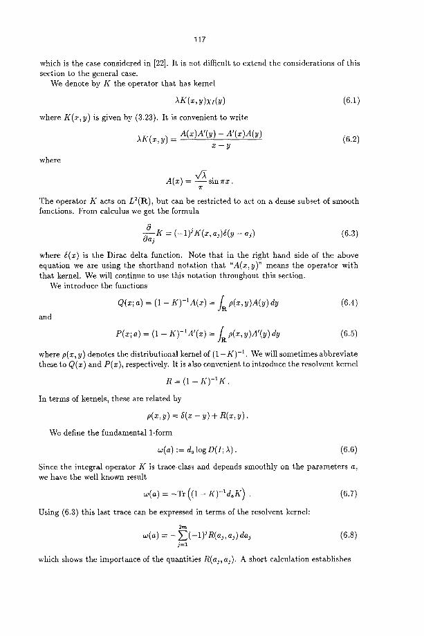
which is the case considered in [22]. It is not difficult to extend the considerations of this section to the general case.

We denote by K the operator that has kernel

.~K(x,y)xt(y) (6.1)

where K(x, y) is given by (3.23). It is convenient to write

Mr(x, y) = a(x)A'(y) - A'(x)A(y) (6.2) x - y

where

A(x) = - - sm 7rx. 7r

The operator K acts on L2(R), but can be restricted to act on a dense subset of smooth functions. From calculus we get the formula

0 - - K = ( -1 ) J K(x , a3)6(y - aj) (6.3) Oaj

where 6(x) is the Dirac delta function. Note that in the right hand side of the above equation we are using the shorthand notation that "A(x,y)" means the operator with that kernel. We will continue to use this notation throughout this section.

We introduce the functions

Q(x; a) = (1 - K)- 'A(x) = .f, p(x, y)A(y) dy (6.4)

and

P(x; a) = (1 - K)-iA'(x) = / I t p(x, y)m'(y) dy (6.5)

where p(x, y) denotes the distributional kernel of (1 - K) -1. We will sometimes abbreviate these to Q(x) and P(x), respectively. It is also convenient to introduce the resolvent kernel

n = ( 1 -

In terms of kernels, these are related by

p(x, y) = ~(x - y) + n (x , y) .

We define the fundamental 1-form

w(a) := d~ log D(I; .~). (6.6)

Since the integral operator K is trace-class and depends smoothly on the parameters a, we have the well known result

w(a) = - T r ((1 - K ) - l d o U ) . (6.7)

Using (6.3) this last trace can be expressed in terms of the resolvent kernel:

2m

w(a) = - ~_,(-1)J R(aj, a j)daj (6.8) j = l

which shows the importance of the quantities R(aj, a j). A short calculation establishes

118

~a~ K) -1 (-1)JR(x, aj)p(aj, y) - =

We will need two commutators which we state as lemmas.

L e m l n a 2 If D = d denotes the differentiation operator, then

2m [D, (1 - K) -I] = - ~--~(-1)/R(x, aj)p(ai, y).

j=l

Proof: Since

(6.9)

[D, (1 - K) -1] = (1 - K) -1 [D, K] (1 - K ) -1 ,

we begin by comput ing [D, K]. An integration by par ts shows tha t

[D, K] = - ~--~(-1)JK(x, aj )~(y - aj ) J

where we used the proper ty

OK(x, Y) + 0 K ( x , y) = 0 Ox Oy

satisfied by our K(x ,y ) and the well known formula for the derivative of XI(x). The ]emma now follows from the fact that

n(x, y) -= ] , p(x, z)U(z, y) dz = ]~ K(x , z)p(z, y) dz .

L e m m a 3 If M~ denotes the multiplication by x operator, then

I/x, (1- 1~-) -1] : Q(X) (1- I ( t ) - lAtxi(y)- ~9(x) (1 - I(t)-IA~I(y)

where K t denotes the transpose of K, and also

[Mx, (1 - K ) - ' ] = (x - y )R(x , y ) .

Proof: We have

[Mx, K] = (A(x)A'(y) - A'(x)A(y)) xI(y) (1 - K ) -1 .

From this last equation the first part of the l emma follows using the definitions of Q and P. The al ternat ive expression for the commuta tor follows direct ly from the definition of p(x, y) and its relationship to R(x, y). •

This l emma leads to a representat ion for the kernel R(x, y) [19]:

L e m m a 4 / f R(x, y) is the resolvent kernel of (6.2) and Q and P are defined by (6.4) and (6.5), respectively, then for x ,y C I we have

R(x, y) Q(x; a)P(y; a) - P(x; a)Q(y; a) = , x # y , x--y

and

119

R(x ,x )= ~x (X;a)P(x;a) -~x (X;a)Q(x;a ).

Proof: Since K(x, y) = K(y, x) we have, on I ,

( 1 - - I(')-IAx1 = ( 1 - I()-IAx, = ( 1 - K ) - I A

(the last since the kernel of K vanishes for y ~ I). Thus (1 - Kt)-IAxz = Q on I, and similarly (1 - Kt)-IA'xI = P on 1. The first part of the lemma then follows from Lemma 3. The expression for the diagonal follows from Taylor's theorem. •

We remark that Lemma 4 used only the property that the kernel K(x, y) can be written as (6.2) and not the specific form of A(x). Such kernels are called "completely integrable integral operators" by Its et. al. [19] and Lemma 4 is central to their work.

B. Derivation of the JMMS Equations

We set

qj=qj (a)= =-olim Q(x;a) and p j=pj (a )= .=_l i~P(x ;a ) , j = l , . . . , 2 m . (6.10) xfil x~I

Specializing Lemma 4 we obtain immediately

R(aj, ak) - - qjPk - - P~q~ aj - - ak

Referring to (6.9) we easily deduce that

and

Thus

Now

Similarly,

, j C k . ( 6 . 1 1 )

Oq.j = (_l)kR(aj,ak)qk, j ¢ k Oa k

OP----i = (--1)kR(aj,ak)pk, j # k. Oak

d._QQ ___ D (1 - K)- ' A(x) dx

= (1 - K) -1 DA(x) + [D, (1 - K) -1] A(x)

= (1 - K) -1A'(x) - ~_,l--1)kR(x, ak)qk. k

~x (aJ; a) = pj -- E(-1)kR(aj , ak)q~. k

d._ffP = (1 - K) -1 A"(x) + [D, (1 - K) -1] A'(x) dz

= _~2 (1 - K ) - ' A(x) - ~ ( - 1 ) k n ( x , ak)p~. k

(6.12)

(6.13)

(6.14)

120

Thus

d P ( ~ ; a) = - ~ % - ~ ( - 1 ) ~ n ( ~ j , a~)p~. (6.15) dx 3 k

Using (6.14) and (6.15) in the expression for the diagonal of R in Lemma 4, we find

n ( ~ , a j ) ~ ~ ~ ~2(-1)~n(aj , (6.16) = 7(" qj +p~ + ak)R(ak, aj)(aj --ak). k

Using

~;" OQ(x; a) OajOq-JJ = dQ ,a)lx_~ + ~ , = ~ ,

(6.12) and (6.14) we obtain

Similarly,

Oqj Oaj = pj - ~ ( - 1 ) k n ( a j ' ak)qk. (6.17)

k¢j

Opj _ Oaj ~r2qj - ~(--1)kR(aj , ak)pk. (6.18)

kgj

Equations (6.11)-(6.13) and (6.16)-(6.18) are the JMMS equations. We remark that they appear in slightly different form in [22] due to the use of sines and cosines rather than exponentials in the definitions of Q and P.

C. Hamiltonian Structure of the JMMS Equations

To facilitate comparison with [22, 35] we introduce

i 1 q2j = - - ~ x 2 j , q 2 j + l ~--- ~ x 2 j A - 1

P ~ j = - - i y 2 j ~ P 2 j + I = Y 2 j + I ,

1

71.2 2m a~(~, y):= - ~ + g - E M~_

4 ~ k=l a j - - a k " k¥3

In this notation,

(6.19)

w(a) = ~ Gj(x, y) daj. J

If we introduce the canonical symplectic structure

{xj,xk} = {Yj, Yk} = O, {xj,yk} = 5jk, (6.20)

then as shown in Moser [35J

T h e o r e m 7 The integrals Gj(x, y) are in involution; that is, if we define the symplectic structure by (6.20) we have

{Gj, Gk}=O forall j , k = l , . . . , 2 m .

Furthermore as can be easily verified, the JMMS equations take the following form [22]:

121

T h e o r e m 8 I f we define the Hamiltonian

2m

~(a) = E as(~, y)das, j= l

then Eqs. (6.12), (6.13), (6.17) and (6.18) are equivalent to Hamilton's equations

d~xj = {x j ,w(a)} and d~yj = {yj ,w(a)} .

In words, the flow of the point (x, y) in the "time variable" aj is given by Hamilton's equations with Hamiltonian Gj.

The (Frobenius) complete integrability of the JMMS equations follows immediately from Theorems 7 and 8. We must show

d ~ { x j , w } = O and d~{yj ,w} =0 .

Now

~o {~,,~) = {~o~J,~) + { ~ s , ~ o ~ } ,

but d,w = 0 since the Gk's are in involution. And we have

{d~xj, w} = E ({{xj, Gk} , Gt} - {{xj, Gt}, Gk}) dak A dae k<£

which is seen to be zero from Jacobi's identity and the involutive property of the Gj's.

D. Reduction to Painlev~ V in the One Interval Case

1. The a(x;,k) differential equation

We consider the case of one interval:

r n = l , a l = - t , a s = t , with s : = 2 t . (6.21)

Since p(x ,y) is both symmetric and even for x ,y E I , we have q2 = - q l and p2 = Pl- Introducing the quantity

f / p ( ) p( )d r 1 -- - t ~ x ex -iTcx x t

we write

~ _ v~ ql = 7 ~ / ( r l - r l ) and pl = -~-(<+~).

Specializing the results of Sec. VI B to m = 1 we ~ have

w(a) = - 2 R ( t , t) dt , (6.22)

1 ~ 2 R ( - t , t ) = -yq ,p~ = ~-~7( , , - ~ ) , (6.23)

dql Oql Oql dt Oal + ~a2 = -Pl + 2 R ( - t , t )ql ,

d--i- = 7r2ql + 2 R ( - t , t)pl ,

dr--A1 = i~rrl + 2 R ( - t , t)V1, (6.24) dt

122

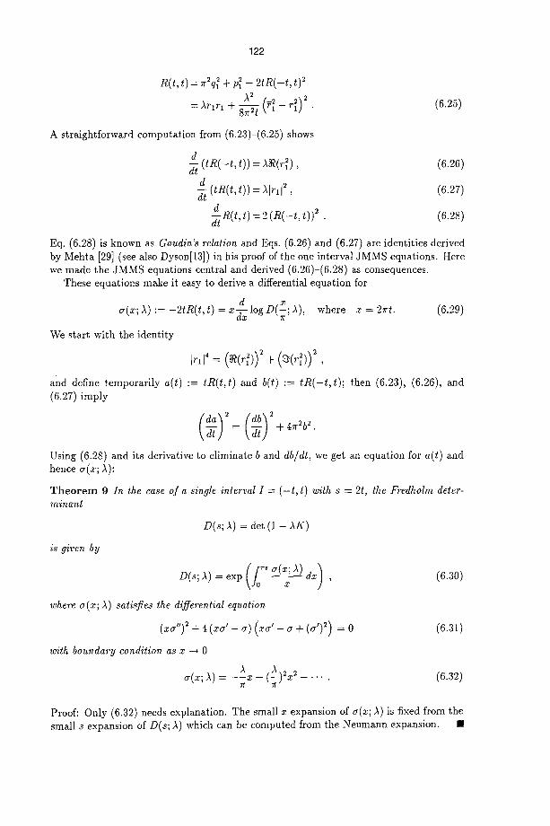
R(t, t) = ~r2q~ + p~ - 2 tR(- t , t) 2

AFlrl + 8 - ~ (F~ - r~) 2 . (6.25)

A straightforward computation from (6.23)-(6.25) shows

d d-t ( tR( - t , t)) = A~(r~), (6.26)

d ( t R ( t , t)) = Alrx[ 2 , (6.27)

d -~ R(t, t) = 2 ( R ( - t , t) ) 2 . (6.28)

Eq. (6.28) is known as Gaudin's relation and Eqs. (6.26) and (6.27) are identities derived by Mehta [29] (see also Dyson[13]) in his proof of the one interval JMMS equations. Here we made the JMMS equations central and derived (6.26)-(6.28) as consequences.

These equations make it easy to derive a differential equation for

a(x; A) := -2 tR( t , t ) = x log D(~; A), where x = 27rt. (6.29)

We start with the identity

Jr iJ ' - - + ,

and define temporarily a(t) := tR(t , t) and b(t) := tR ( - t , t ) ; then (6.23), (6.26), and (6.27) imply

at ] = \ g i ] + 4~b~ "

Using (6.28) and its derivative to eliminate b and db/dt, we get an equation for a(t) and hence a(x; A):

T h e o r e m 9 In the case of a single interval I -= ( - t , t) with s = 2t, the Fredholm deter- minant

is given by

D(s; A) = det (1 - AK)

D(s;A) =exp (fo~" ~r(x"A) dz)

where a(x; A) satisfies the differential equation

(x~r") 2 + 4 (xa' - ~) ( x # - a + (a') 2) = 0

with boundary condition as x --* 0

° ( 5 ; A) = - 7 x - ( ) ~ . . . .

(6.30)

(6.31)

Proof: Only (6.32) needs explanation. The small x expansion of ~r(x; A) is fixed from the small s expansion of D(s; A) which can be computed from the Neumann expansion. •

(6.32)

123

The differential equation (6.31) is the "a representation" of the Painlev$ V equation. This is discussed in [22], and in more detail in Appendix C of [21]. In terms of the monodromy parameters 01 (i = 0, l, ~ ) of [21], (6.31) corresponds to 00 = 01 = 0~ = 0 which is the case of no local monodromy. For an introduction to Painlev$ functions see [20, 24].

2. The a+(x; A) equations

Recalling the discussion following Eq. (3.31), we see we need the determinants D±(s; ~) to compute E~(n; s) for/3 = 1 and 4. Let R~ denote the resolvent kernels for the operators

l ± J K + J K± := = K 1----- , 2 2

where (J f ) (x) = f ( - z ) and the last equality of the above equation follows from the evenness of K. Thus

R± := (1 - K+)-IK± = 1(1 ± J)R ,

which in terms of kernels is

n±(x, y) = ~ (R(x, y) ± n(-x, y)).

Thus

1 d t) ( n _ ( t , t ) - n + ( t , t ) ) ~ = ( n ( - t , t ) ) ~ = ~ - ~ n ( t , .

Introducing the analogue of a(x; A), i.e.

a±(x;A) := x d x log D~(;; ~),

the above equation becomes

d (6.33) t ] x dx x

Of course, a+(x; A) also satisfy

a+(x; ~) + a_(x; ~) = or(x; ),). (6.34)

Using (6.33) and (6.34) and integrating a.(x; A)/x we obtain (the square root sign ambi- guity can be fixed from small x expansions)

T h e o r e m 10 Let D±(s; )~) be the Fredholm determinants defined by (3.31), then

l ogD+(s ;£ )= l o g D ( s ; A ) ± 2 f 0 - - ~ x 21°gD(x;A)dx" (6.35)

124

VII. ASYMPTOTICS

A. Asymptotics via the Painlev~ V Representation

In this section we explain how one derives asymptotic formulas for Ez(n; s) as s ~ starting with the Painlev~ V representations of Theorems 9 and 10. This section follows Basor, Tracy and Widom [4] (see also [31]). We remark that the asymptotics of E~(0; s) as s ---* cc was first derived by Dyson [12] by a clever use of inverse scattering methods.

Referring to Theorems 9 and 10 one sees that the basic problem from the differential equation point of view is to derive large x expansions for

g0(x) := g(x; 1) (7.1)

°~g 1), ~=1,2, . . . (7.2) ~(~) := ~5-z(~; 0~g±" 1), n 1,2, (7.3) g±,~(~) := ~ - : (x ; . . . . .

We point out the sensitivity of these results to the parameter A being set to one. This dependence is best discussed in terms of the differential equation (6.31) where it is an instance of the general problem of connection formulas, see e.g. [24] and references therein. In this context the problem is: given the small x boundary condition, find asymptotic formulas as x --~ cc where all constants not determined by a local analysis at oc are given as functions of the parameter A. If we assume an asymptotic solution for large x of the form g(x) ~ ax p, then (6.31) implies either p = 1 or 2 and if p = 2 then necessarily a = -¼. The connection problem for (6.31) has been studied by McCoy and Tang [26] who show that for 0 < A < 1 one has

as x --* ~ with

~(x,A) = a(~)z + b(~) + o ( 1 )

1 1 a(A) = log(1 - A) and ~(A) = ~a:(A).

7I"

Since these formulas make no sense at A = 1, it is reasonable to guess that

-!x~. (7.4) g(x;1)~ 4

For a rigorous proof of this fact see [43]. It should be noted that in Dyson's work he too "guesses" this leading behavior to get his asymptotics to work (this leading behavior is not unexpected from the continuum Coulomb gas approximation). Given (7.4), and only this, it is a simple matter using (6.31) to compute recurs±rely the correction terms to this leading asymptotic behavior:

1 ~= ~-~'c~ (7.5) g 0 ( x ) = - 4 x 2 - + x--*c~

(c2 = --¼, c4 = -~ , etc.). Using (7.5) in (6.30) and (6.35) one can efficiently generate the large s expansions for D(s; 1) and D±(s; 1) except for overall multiplicative constants. In this instance other methods fix these constants (see discussion in [4, 27]). In general this overall multiplicative constant in a T-function is quite difficult to determine (for an example of such a determination see [2, 3]). We record here the result:

log D±(s; 1 ) = - l~ r~s2 :F l~r~ - ~ log ~rs 4- 41- log 2 1 + ~ log 2 + 23-('(-1)+ o(1)(7.6)

125

as s --+ oo where ( is the Riemann zeta function. We mention that for 0 < ~ < 1 the asymptotics of D(s; ~) as s -+ ~ are known [5, 26].

One method to determine the asymptotics of as(x) as x --~ oo is to examine the variational equations of (6.31), i.e. simply differentiate (6.31) with respect to A and then set A = 1. These linear differential equations can be solved asymptotically given the asymptotic solution (7.5). In carrying this out one finds there are two undetermined constants corresponding to the two linearly independent solutions to the first variational equation of (6.31). One constant does not affect the asymptotics of a l (x) (assuming the other is nonzero!). Determining these constants is part of the general connection problem and it has 'not been solved in the context of differential equations. In [4, 43] Toeplitz and Wiener-Hopf methods are employed to fix these constants. The Toeplitz arguments of [4] depend upon some unproved assumptions about scaling limits, but the considerations of [43] are completely rigorous and we deduce the following result [4] for (r~(x) for all n = 3 ,4 , . . . :

n! exp(nx) [ ~ [1 g(Tn-1 4)1_. + 1_~(7n7 2 _ 16) 1 ±1 (7.7)

as x --~ oo. For n --- 1, 2 the above is correct for the leading behavior but for n = 1 the correction terms have coefficients ~ and i~s, respectively, and for n = 2 the above formula gives the coefficient for 1/z but the coefficient for 1/x 2 is ~ . See [4] for asymptotic formulas for o±,,~(X ).

Since the asymptotics of EZ(0; s) are known, it is convenient to introduce

E~(n; s) r~(n; s ) . - E z ( 0 ; ~)"

Here we restrict our discussion to fl = 2 (see [4] for other cases). Using (7.7) in (3.29) one discovers that there is a great deal of cancellation in the terms which go into the asymptotics of r2(n; s). To prove a result for all n E N by this method we must handle all the correction terms in (7.7)--this was not done in [4] and so the following result was proved only for 1 < n < 10:

r2(n; s) = 2,n 1 + + + 1~(4n4 + 48n 2 -}- 229) + O( )

(7.8)

where

B 2 , . = 2 - " ~ - ~ / % -~"~÷"~/2 (~ - 1)! (~ - 2)! . . . 2! 1 ! .

In the next section we derive the leading term of (7.8) for all n C N. Asymptotic formulas for rz(n;s) (/3 = 1,4,4-) can be found in [4].

B. Asymptotics of r2(n; s) from Asymptotics of Eigenvalues

The asymptotic formula (7.8) can also be derived by a completely different method (as was briefly indicated in [4]). If we denote the eigenvalues of the integral operator K by .k0 > ~1 > "'" > 0, then

o o

det (1 - AK) = 1-I(1 - AA,), i=O

126

and so it follows immedia te ly from (3.29) that

r2(n;s) : ~ ia ' ' " hln Y~ (1 - h i , ) . . . ( 1 - AI.) " (7.9)

i~ < ' " < i n

(This is formula (5.4.30) in [27].) Thus the asymptotics of the eigenvalues hi as s --+ oo can be expected to give information on the asymptotics of r2(n; s) as s --+ oo.

It is a remarkable fact that the integral operator K , acting on the interval ( - t , t ) , commutes with the differential operator £ defined by

d t2)dd@ + t2x2f, s 2t; (7.10) £ f = ~xx(X~ _ =

the boundary condition here is that f be continuous at + t . Thus the integral operator and the differential operator have precisely the same eigenfunct ions-- the so-called prolate spheroidal wave functions, see e.g. [33]. Now Fuchs [15], by an application of the W K B method to the differential equation, and using a connection between the eigenvalues A~ and the values of the normalized eigenfunctions at the end-points, derived the asymptot ic formula

1 - hl ~ ~ri+1221+312si+1/2e-~/i! (7.11)

valid for fixed i as s ~ ~z. Further terms of the asymptotic expansion for the ratio of the two sides were obtained by Slepian [40].

If one looks at the asymptotics of the individual terms on the right side of (7.9), then we see from (7.11) that they all have the exponential factor e ~ and that the powers of s that occur are

s-~12-(i~ +--.+i,).

Thus the te rm corresponding to i~ = 0, i2 = 1, . . . , i= = n - 1 dominates each of the others• In fact we claim this term dominates the sum of all the others, and so

r2(n; s) ~ 1! 2! . . . (n - 1)! ~r-~C"+l)/22-"'-~/2s-"2/2e'~, (7.12)

in agreement with (7.8). To prove this claim, we write

Ai0"" .~io r2(n;s) = (1 - AO). . - (1 - ho)

+ ~ , h h . " h i .

(I - hq)-.. (1 - h i . )

• ' '0 where ,0 = 0, z ° = 1 , . . . , z= = n - 1 and the sum here is taken over all ( i l , . . . , i , ) ( io , . . . , i o) with il < " " < i~. We have to show that

(1 - h~ , ) (1 - h ~ . ) / ~ - ' / , ~ 0

as s ~ co and we know that this would be true if the sum were replaced by any summand. Write ~ ' = ~21 + ~2 where in Y21 we have ij < N for all j (N to be determined later) and ~ a is the rest of ~2'. Since ~21 is a finite sum we have

enTrs

so we need consider only ~2. In any summand of this we have ij _> N for some j , and so for this j

127

and by (7.11) this is at most

1 1

1 - A b - 1 - A N

aN 8-N-l~ 2 erS

for some constant a N , The product of all other factors

1

1 - A 6

appearing in this summand is at most

and so by (7.11) with i = 0 at most

b~ s -(n-x)/2 e (~-l)~s

for another constant bn. So we have the es t imate

E 2 <~ aNbn 8-N-n/2 en~rs E ~il "'" ~in

where the sum on the right may be taken over all n-tuples ( i x , . . . , Q ) . precisely equal to (tr K) ~ = s ~. Hence

E 2 <- aNbn'S-N+n/2enrS "

If we choose N > (n 2 -4- n)/2 then we have

gnats EJ: o

as desired.

This sum is

C. Dyson's Continuum Model

In [13] Dyson constructs a continuum Coulomb gas model [27] for Ep(n;s). In this cont inuum model,

E~(n; s) = exp ( - f lW- (1- ~)S)

where

is the total energy,

t S = ] p(:) log p(:) dx

is the entropy, ~(x) = p(x) - I and p(x) is a continuum charge distribution on the line satisfying p(.) -~ I as • -~ +oo and p(x) >__ 0 everywhere. The distribution p(.) is chosen to minimize the free energy subject to the condition

128

/2 , /2 p ( z ) d z = n .

Analyzing his solution in the limit 1 < < n < < s, Dyson finds E~(n;s) ,,. exp(-/3Wc) where

7r2s2~rs l n ( n l n ( n 2~)[log(~-~)+ 1] (7.13) W e - 16 ~ (n+~5)+ + 3 ) + +

with ~ = 1/2 - 1~ft. We now compare these predictions of the continuum model with the exact results.

First of all, this continuum prediction does not get the s -1/4 (for fl = 2) or the s -1/s (for /3 = 1,4) present in all Ez(n;s) that come from the log~rs term in (7.6). Thus it is better to compare with the continuum prediction for rz(n;s). We find that the continuum model gives both the correct exponential behavior and the correct power of s for all three ensembles. Tracing Dyson's arguments shows that the power of s involving the n 2 exponent is an enewy effect and the power of s involving the n exponent is an entropy effect. Finally, the continuum model also makes a prediction (for large n) for the the BZ,~'s (B2,~ is given above). Here we find that the ratio of the exact result to the continuum model result is approximately n -1/1~ for/3 = 2 and n -1/24 for/3 = 1,4. This prediction of the continuum model is better than it first appears when one considers that the constants themselves are of order n ~2/2 (/3 = 2) and n ~2 (/3 = 1,4).

ACKNOWLEDGMENTS

It is a pleasure to acknowledge E. L. Basor, P. Diaconis, F. J. Dyson, P. J. Forrester, P. B. Kahn, M. L. Mehta~ and P. Nevai for their many helpful comments and their encouragement. We also thank F. J. Dyson and M. L. Mehta for sending us their preprints prior to publication. The first author thanks the organizers of the 8 *h Scheveningen Conference, August 16-21, 1992, for the invitation to attend and speak at this conference. These notes are an expanded version of the lectures presented there. This work was supported in part by the National Science Foundation, DMS-9001794 and DMS-9216203, and this support is gratefully acknowledged.

REFERENCES

[1] R. Balian, Random matrices and information theory, Nuovo Cimento B57 (1968) 183-193.

[2] E. L. Basor and C. A. Tracy, Asymptotics ofa tau-function and Toeplitz determinants with singular generating functions, Int. J. Modern Physics A 7, Suppl. 1A (1992) 83- 107.

[3] E. L. Basor and C. A. Tracy, Some problems associated with the asymptotics of "c-functions, Surikagaku (Mathematical Sciences) 30, no. 3 (1992) 71-76 [English translation appears in RIMS-845 preprint].

[4] E. L. Basor, C. A. Tracy, and H. Widom, Asymptotics of level spacing distribution functions for random matrices, Phys. Rev. Letts. 69 (1992) 5-8.

[5] E. L. Basor and H. Widom, Toeplitz and Wiener-Hopf determinants with piecewise continuous symbols, J. Func. Analy. 50 (1983) 387-413.

129

[6] M. 3. Bowick and g. Br4zin, Universal scaling of the tail of the density of eigenvalues in random matrix models, Phys. Letts. B268 (1991) 21-28.

[7] E. Br4zin and V. A. Kazakov, Exactly solvable field theories of closed strings, Phys. Letts. B236 (1990) 144-150.

[8] P. Diaconis and M. Shahshahani, The subgroup algorithm for generating uniform random variables, Prob. in the Engin. and Inform. Sci. 1 (1987) 15-32.

[9] M. Douglas and S. H. Shenker, Strings in less than one dimension, Nucl. Phys. B335 (1990) 635-654.

[i0] F. J. Dyson, Statistical theory of energy levels of complex systems, l, ll, and Ill, J. Math. Phys. 3 (1962) 140-156; 157-165; 166-175.

[11] F. J. Dyson, The three fold way. Algebraic structure of symmetry groups and ensem- bles in quantum mechanics, J. Math. Phys. 3 (1962) 1199-1215.

[12] F. J. Dyson, Fredholm determinants and inverse scattering problems, Commun. Math. Phys. 47 (1976) 171-183.

[13] F. J. Dyson, The Coulomb fluid and the fifth Painlev4 transcendent, IASSNSS-HEP- 92/43 preprint.

[14] D. Fox and P. B. Kahn, Identity of the n-th order spacing distributions for a class of Hamiltonian unitary ensembles, Phys. Rev. 134 (1964) 1151-1155.

[15] W. H. J. Fuchs, On the eigenvalues of an integral equation arising in the theory of band-limited signals, J. Math. Anal. and Applic. 9 (1964) 317-330.

[16] D. J. Gross and A. A. Migdal, Nonperturbative two-dimensional quantum gravity, Phys. Rev. Letts. 64 (1990) 127-130; A nonperturbative treatment of two-dimensional quantum gravity, Nucl. Phys. B340 (1990) 333-365.

[17] D. J. Gross, T. Piran, and S. Weinberg, eds., Two Dimensional Quantum Gravity and Random Surfaces (World Scientific, Singapore, 1992).

[18] L. g. Hua, Harmonic analysis of functions of several complex variables in the classical domains [Translated from the Russian by L. Ebner and A. Koranyi] (Amer. Math. Soc., Providence, 1963).

[19] A. R. Its, A. G. Izergin, V. E. Korepin, and N. A. Slavnov, Differential equations for quantum correlation functions, Int. J. Mod. Physics B 4 (1990) 1003-1037.

[20] K. Iwasaki, H. Kimura, S. Shimomura, and M. Yoshida, From Gauss to Painlevd: A Modern Theory of Special Functions (Vieweg, Braunschweig, 1991).

[21] M. Jimbo and T. Miwa, Monodromy preserving deformation of linear ordinary dif- ferential equations with rational coefficients. II, Physica 2D (1981) 407-448.

[22] M. Jimbo, T. Miwa, Y. M6ri, and M. Sato, Density matrix of an impenetrable Bose gas and the fifth Painlev4 transcendent, Physica 1D (1980) 80-158.

[23] R. D. Kamien, H. D. Politzer, and M. B. Wise, Universality of random-matrix pre- dictions for the statistics of energy levels, Phys. Rev. Letts. 60 (1988) 1995-1998.

[24] D. Levi and P. Winternitz, eds., Painlev6 Transcendents: Their Asymptotics and Physical Applications (Plenum Press~ New York, 1992).

[25] D. S. Lubinsky, A survey of general orthogonal polynomials for weights on finite and infinite intervals, Acta Applic. Math. 10 (1987) 237-296.

[26] B. M. McCoy and S. Tang, Connection formulae for Painlev4 V functions, Physica 19D (1986) 42-72; 20D (1986) 187-216.

[27] M. L. Mehta, Random Matrices, 2nd edition (Academic, San Diego, 1991). [28] M. L. Mehta~ Power series for level spacing functions of random matrix ensembles,

Z. Phys. B 86 (1992) 285-290. [29] M. L. Mehta, A non-linear differential equation and a Fredholm determinant, J. de

Phys. I France, 2 (1992) 1721-1729.

130

[30] M. L. Mehta and G. Mahoux, A method of integration over matrix variables: III, Indian J. pure appl. Math., 22(7) (1991) 531-546.

[31] M. L. Mehta and G. Mahoux, Level spacing functions and non-linear differential equations, preprint.

[32] G. Mahoux and M. L. Mehta, A method of integration over matrix variables: IV, J. Phys. I France 1 (1991) 1093-1108.

[33] J. Meixner and F. W. Sch~fke, Mathieusche Funktionen und Sphffroidfunktionen (Springer Verlag, Berlin, 1954).

[34] G. Moore, Matrix models of 2D gravity and isomonodromic deformation, Prog. Theor. Physics Suppl. No. 102 (1990) 255-285.

[35] J. Moser, Geometry of quadrics and spectral theory, in Chern Symposium 1979 (Springer, Berlin, 1980), 147-188.

[36] T. Nagao and M. Wadati, Correlation functions of random matrix ensembles related to classical orthogonaJ polynomials, J. Phys. Soc. Japan 60 (1991) 3298-3322.

[37] P. Nevai, Asymptotics for orthogonal polynomials associated with exp(-x4), SIAM J. Math. Anal. 15 (1984) 1177-1187.

[38] L. A. Pastur, On the universality of the level spacing distribution for some ensembles of random matrices, Letts. Math. Phys. 25 (1992) 259-265.

[39] C. E. Porter, Statistical Theory of Spectra: Fluctuations (Academic, New York, 1965). [40] D. Slepian, Some asymptotic expansions for prolate spheroidal wave functions, J.

Math. Phys. 44 (1965) 99-140. [41] A. D. Stone, P. A. Mello, K. A. Muttalib, and J.-L. Pichard, Random matrix theory

and maximum entropy models for disordered conductors, in Mesoscopic Phenomena in Solids, eds. B. L. Altshuler, P. A. Lee, and R. A. Webb (North-Holland, Amster- dam, 1991), Chp. 9, 369-448.

[42] H. Weyl, The Classical Groups (Princeton, Princeton, 1946). [43] H. Widom, The asymptotics of a continuous analogue of orthogonal polynomials, to

appear in J. Approx. Th.