lecture notes on random matrices - mathematisches …lerdos/ss09/random/... · 2009-03-01 ·...
TRANSCRIPT

Lecture notes on random matrices
Greg W. AndersonDepartment of Mathematics
University of Minnesota
Alice GuionnetENS Lyon
Ofer ZeitouniUniversity of Minnesota and Technion
30 November, 2006c©Greg W. Anderson, Alice Guionnet, Ofer Zeitouni
(2004–2006).Do not distribute without the written permission of author.
Rather rough - Comments welcomed!
Contents
1 Random matrices and eigenvalues 8
1.1 Eigenvalues . . . . . . . . . . . . . . . . . . . . . . . . . . . 8
2 Real and Complex Wigner matrices 10
2.1 Real Wigner matrices: traces, moments and combinatorics . 10
2.1.1 The semicircle distribution, Catalan numbers, andDyck paths . . . . . . . . . . . . . . . . . . . . . . . 11
2.1.2 Proof #1 of Wigner’s Theorem 2.1.4 . . . . . . . . . 14
2.1.3 Proof of Lemma 2.1.12 : Words and Graphs . . . . . 16
2.1.4 Proof of Lemma 2.1.13 : Sentences and Graphs . . . 20
2.1.5 Some useful approximations . . . . . . . . . . . . . . 24
2.1.6 Maximal eigenvalues and Furedi-Komlos enumeration 26
2.1.7 Central limit theorems for moments . . . . . . . . . 33
2.2 Complex Wigner matrices . . . . . . . . . . . . . . . . . . . 39
2.3 Concentration for functional of random matrices and loga-rithmic Sobolev inequalities . . . . . . . . . . . . . . . . . . 41
2.3.1 Smoothness properties of linear functions of the em-pirical measure . . . . . . . . . . . . . . . . . . . . . 41
2.3.2 Concentration inequalities for independent variablessatisfying logarithmic Sobolev inequalities . . . . . . 42
2.3.3 Concentration for Wigner-type matrices . . . . . . . 45
2.4 Stieltjes transforms and recursions . . . . . . . . . . . . . . 46
2.4.1 Gaussian Wigner matrices . . . . . . . . . . . . . . . 48
2.4.2 General Wigner matrices . . . . . . . . . . . . . . . 50
2

3
2.5 Joint distribution of eigenvalues in the GOE and the GUE . 53
2.5.1 Definition and preliminary discussion of the GOE andthe GUE . . . . . . . . . . . . . . . . . . . . . . . . 53
2.5.2 Proof of the joint distribution of eigenvalues . . . . . 55
2.5.3 Selberg’s integral formula and proof of (2.5.4) . . . . 59
2.5.4 Joint distribution of eigenvalues - alternative formu-lation . . . . . . . . . . . . . . . . . . . . . . . . . . 66
2.6 Large deviations for random matrices . . . . . . . . . . . . 67
2.6.1 Large deviations for the empirical measure . . . . . 68
2.6.2 Large deviations for the top eigenvalue . . . . . . . . 78
2.7 Bibliographical notes . . . . . . . . . . . . . . . . . . . . . . 82
3 Orthogonal polynomials, spacings, and limit distributionsfor the GUE 85
3.1 Summary of main results: spacing distributions in the bulkand edge of the spectrum for the GUE . . . . . . . . . . . . 85
3.2 Hermite polynomials and the GUE . . . . . . . . . . . . . . 87
3.2.1 The Hermite polynomials and harmonic oscilators . 88
3.2.2 Connection with the GUE . . . . . . . . . . . . . . . 90
3.3 The semicircle law revisited . . . . . . . . . . . . . . . . . . 94
3.3.1 Calculation of moments of LN . . . . . . . . . . . . 95
3.3.2 The Harer-Zagier recursion and Ledoux’s argument . 96
3.4 Quick introduction to Fredholm determinants . . . . . . . . 100
3.4.1 The setting, fundamental estimates, and definition ofthe Fredholm determinant . . . . . . . . . . . . . . . 100
3.4.2 Definition of the Fredholm adjugants, Fredholm re-solvents, and a fundamental identity . . . . . . . . . 104
3.5 Gap probabilities at 0 and proof of Theorem 3.1.1. . . . . . 109
3.5.1 The method of Laplace . . . . . . . . . . . . . . . . 110
3.5.2 Evaluation of the scaling limit - proof of Lemma 3.5.2 112
3.5.3 A complement: determinantal relations . . . . . . . 114
3.6 Analysis of the sine-kernel . . . . . . . . . . . . . . . . . . . 116
3.6.1 General differentiation formulae and the Kyoto equa-tions . . . . . . . . . . . . . . . . . . . . . . . . . . . 116

4
3.6.2 Derivation of the Kyoto equations: proof of Theorem3.6.2 . . . . . . . . . . . . . . . . . . . . . . . . . . . 121
3.6.3 Reduction of the Kyoto equations to Painleve V . . 123
3.7 Edge-scaling: Proof of Theorem 3.1.7 . . . . . . . . . . . . . 126
3.7.1 A preliminary view of the Airy function . . . . . . . 126
3.7.2 Vague convergence of the rescaled largest eigenvalue:proof of Theorem 3.1.7 . . . . . . . . . . . . . . . . . 127
3.7.3 Steepest descent: proof of Lemma 3.7.8 and proper-ties of the Airy function . . . . . . . . . . . . . . . . 129
3.8 Analysis of the Tracy-Widom distribution and proof of The-orem 3.1.10 . . . . . . . . . . . . . . . . . . . . . . . . . . . 137
3.8.1 The first standard moves of the game . . . . . . . . 138
3.8.2 The wrinkle in the carpet . . . . . . . . . . . . . . . 139
3.8.3 Linkage to Painleve II . . . . . . . . . . . . . . . . . 141
3.9 Bibliographical notes . . . . . . . . . . . . . . . . . . . . . . 142
4 Some generalities 144
4.1 Joint distribution of eigenvalues in the classical matrix en-sembles . . . . . . . . . . . . . . . . . . . . . . . . . . . . . 144
4.1.1 Manifolds and the coarea formula . . . . . . . . . . . 144
4.1.2 Measures of spheres . . . . . . . . . . . . . . . . . . 149
4.1.3 Measures of unitary groups . . . . . . . . . . . . . . 150
4.1.4 Measures of flag manifolds . . . . . . . . . . . . . . . 152
4.1.5 The trace-of-powers map . . . . . . . . . . . . . . . 153
4.1.6 Lie groups and an integration formula of Weyl type 155
4.1.7 Applications of the Weyl integration formula . . . . 159
4.1.8 The Gaussian ensembles . . . . . . . . . . . . . . . . 161
4.1.9 The Laguerre ensemble . . . . . . . . . . . . . . . . 162
4.1.10 The Jacobi ensemble . . . . . . . . . . . . . . . . . . 164
4.1.11 Reference notes . . . . . . . . . . . . . . . . . . . . . 165
4.2 Determinantal processes . . . . . . . . . . . . . . . . . . . . 166
4.2.1 Basic definitions . . . . . . . . . . . . . . . . . . . . 166
4.2.2 Determinantal projections . . . . . . . . . . . . . . . 171
4.2.3 Properties of determinantal processes, and the CLT 175

5
4.2.4 Translation invariant determinantal processes . . . . 177
4.2.5 One dimensional translation invariant determinantalprocesses . . . . . . . . . . . . . . . . . . . . . . . . 182
4.2.6 Convergence issues . . . . . . . . . . . . . . . . . . . 185
4.2.7 Examples . . . . . . . . . . . . . . . . . . . . . . . . 188
4.3 Stochastic analysis for random matrices . . . . . . . . . . . 193
4.3.1 Dyson’s Brownian motion . . . . . . . . . . . . . . . 193
4.3.2 Proof #7 of Wigner’s Theorem 2.1.4 . . . . . . . . . 203
4.3.3 Central limit theorem . . . . . . . . . . . . . . . . . 214
4.4 Concentration inequalities for random matrices . . . . . . . 220
5 Free probability 221
5.1 Introduction . . . . . . . . . . . . . . . . . . . . . . . . . . . 221
5.2 Non-commutative laws and noncommutative probability spaces221
5.2.1 Algebraic noncommutative probability spaces and laws221
5.2.2 C∗- noncommutative probability spaces and weak topol-ogy . . . . . . . . . . . . . . . . . . . . . . . . . . . . 225
5.2.3 W∗-noncommutative probability spaces . . . . . . . 243
5.3 Free independence . . . . . . . . . . . . . . . . . . . . . . . 247
5.3.1 Independence and free independence . . . . . . . . . 247
5.3.2 Free independence and combinatorics . . . . . . . . 250
5.3.3 Consequence of free independence: free convolution . 256
5.3.4 Free central limit theorem . . . . . . . . . . . . . . . 267
5.3.5 Link with random matrices . . . . . . . . . . . . . . 268
Appendix 277
A Linear algebra preliminaries . . . . . . . . . . . . . . . . . . 277
A.1 Identities and bounds . . . . . . . . . . . . . . . . . 277
A.2 Perturbations for normal and Hermitian matrices . . 278
A.3 Brief review of resultants and discriminants . . . . . 279
B Topological Preliminaries . . . . . . . . . . . . . . . . . . . 280
B.1 Generalities . . . . . . . . . . . . . . . . . . . . . . . 280
B.2 Topological Vector Spaces and Weak Topologies . . 283
B.3 Banach and Polish Spaces . . . . . . . . . . . . . . . 284

6
C Probability measures on Polish spaces . . . . . . . . . . . . 286
C.1 Generalities . . . . . . . . . . . . . . . . . . . . . . . 286
C.2 Weak Topology . . . . . . . . . . . . . . . . . . . . . 287
D Basic notions of large deviations . . . . . . . . . . . . . . . 289
E The skew field H of quaternions, and matrix terminology in F292
E.1 Matrix terminology in F . . . . . . . . . . . . . . . . 293
E.2 The •-construction . . . . . . . . . . . . . . . . . . . 295
E.3 Matrix factorization theorems . . . . . . . . . . . . . 296
E.4 The spectral theorem and key corollaries . . . . . . . 296
E.5 Proof of the spectral theorem . . . . . . . . . . . . . 298
E.6 Some specialized results on projectors . . . . . . . . 299
F Manifolds embedded in Euclidean space . . . . . . . . . . . 301
G Appendix on Operators algebras . . . . . . . . . . . . . . . 305
G.1 Basic definitions . . . . . . . . . . . . . . . . . . . . 305
G.2 Spectral properties . . . . . . . . . . . . . . . . . . . 307
G.3 States and positivity . . . . . . . . . . . . . . . . . 309
G.4 von Neumann algebras . . . . . . . . . . . . . . . . 309
G.5 Non-commutative functional calculus . . . . . . . . . 310
G.6 Riesz representation Theorem . . . . . . . . . . . . . 311
H Stochastic calculus notions . . . . . . . . . . . . . . . . . . . 311
References 315
Notations - This will move
M1(S) − space of probability measures on a topological space S
C(S), Cb(S) − Space of continuous (bounded) functions on S
〈µ, f〉 −∫f(x)µ(dx) , for f measurable , µ ∈M1(S) .
ε(σ) − the signature of a permutation σ
det(M) =∑
ε(σ)∏
Mi,ε(i)where the sum runs over all permutation of {1, · · · , n}.
Unless stated otherwise, for S a Polish space, M1(S) is given the topologyof weak convergence, that makes it into a Polish space.
When we write a(s) ∼ b(s), we assert that there exists c(s) defined fors � 0 such that lims→∞ c(s) = 1 and c(s)a(s) = b(s) for s � 0. We usethe notation an ∼ bn for sequences in the analogous sense.
7

Chapter 1
Random matrices andeigenvalues
Throughout this book, we let H(1)N be the space of (real) symmetric N by
N matrices, and let H(2)N be the space of (complex) Hermitian N by N
matrices. One can always consider H(β), β = 1, 2, as a submanifold of anappropriate Euclidean space, and equip it with the induced topology.
1.1 Eigenvalues
Our interest will be in the study of eigenvalues of matrices in H(β)N . For
H ∈ H(β)N let λ1(H) ≤ · · · ≤ λN (H) be the eigenvalues of H . The following
lemma assures that the eigenvalues are continuous functions in H , andhence can be treated as random variables as soon as a probability measureis put on H(β). For a strengthening of this result, see Appendix A.2.
Lemma 1.1.1 For i = 1, . . . , N , the eigenvalue λi(H) is a continuous (anda fortiori measurable) function of H.
Proof: For H ∈ H(β)N put ‖H‖ :=
√TrH2, thus defining a Euclidean
metric on H(β)N . Note that ‖H‖ ≥ max(λN (H),−λ1(H)). For any positive
integer k we have
λN (H) + ‖H‖ ≤ k
√Tr(H + ‖H‖I)k ≤ k
√N(λN (H) + ‖H‖),
8

9
hence∣∣∣∣
k
√Tr(H + ‖H‖)k − ‖H‖I − λN (H)
∣∣∣∣ ≤ 2(k√N − 1)‖H‖,
and hence
λN (H) = limk→∞
k
√Tr(H + ‖H‖I)k − ‖H‖
uniformly on compact subsets of H(β)N , which proves continuity of λN (·).
Continuity of λi+1(·), . . . , λN (·) granted, by a similar analysis we have
λi(H) = limk→∞
Tr(H + ‖H‖I)k −
N∑
j=i+1
(λj(H) + ‖H‖)k
1/k
− ‖H‖
uniformly on compact subsets of H(β)N , which proves continuity of λi(·). ut
Add here that in fact C∞ in (open) region where eigenvalues
are distinct.

Chapter 2
Real and Complex Wignermatrices
2.1 Real Wigner matrices: traces, momentsand combinatorics
We introduce in this section a basic model of random matrices. Nowhere dowe attempt to provide the weakest assumption of sharpest results available.We point out in the bibliographical notes (Section 2.7) some places wherethe interested reader can find finer results.
Start with two independent families of i.i.d., zero mean, real valuedrandom variables {Zi,j}1≤i<j and {Yi}1≤i, such that EZ2
1,2 = 1 and, for allinteger k ≥ 1,
rk := max(E|Z1,2|k, E|Y1|k
)<∞ . (2.1.1)
Consider the (symmetric) N ×N matrix XN with entries
XN (j, i) = XN(i, j) =
{Zi,j/
√N , if i < j,
Yi/√N , if i = j.
(2.1.2)
We call such a matrix a Wigner matrix, and if the random variables Zi,j
and Yi are Gaussian, we use the term Gaussian Wigner matrix. The case ofGaussian Wigner matrices in which EY 2
1 = 2 is of particular importance,and for reasons that will become clearer in Chapter 3, such matrices arereferred to as GOE (Gaussian Orthogonal Ensemble) matrices.
Let λNi denote the (real) eigenvalues of XN , with λN
1 ≤ λN2 ≤ . . . ≤ λN
N ,and define the empirical distribution of the eigenvalues as the probability
10

11
measure on R defined by
LN =1
N
N∑
i=1
δλNi.
Define the standard semicircle distribution as the probability distribu-tion σ(x)dx on R with density
σ(x) =1
2π
√4 − x21|x|≤2 . (2.1.3)
The following theorem, contained in [Wig55], can be considered the startingpoint of Random Matrix Theory (RMT).
Theorem 2.1.4 (Wigner) For a Wigner matrix, the empirical measureLN converges weakly, in probability, to the standard semicircle distribution.
The statement in Theorem 2.1.4 is that for any f ∈ Cb(R), and any ε > 0,
limN→∞
P (|〈LN , f〉 − 〈σ, f〉| > ε) = 0 .
Remark 2.1.5 The assumption (2.1.1) that rk <∞ for all k is not reallyneeded, see Theorem 2.1.46 in Section 2.1.5.
We will see many proofs of Wigner’s Theorem 2.1.4. In this section, wegive a direct combinatorics based proof, mimicking the original argumentof Wigner. Before doing so, however, we need to discuss some properties ofthe semicircle distribution.
2.1.1 The semicircle distribution, Catalan numbers, andDyck paths
Define the moments mk := 〈σ, xk〉 . By symmetry, m2k+1 = 0. Recall theCatalan numbers1
Ck =
(2kk
)
k + 1.
1There is a slight ambiguity in the literature concerning the numbering of Catalannumbers. Thus, [Aig79, Pg 85] denotes by ck what we denote by Ck−1. Our notationsfollow [Sta97].

12
A calculus exercise in integration by parts shows that m2k = Ck: indeed,
m2k =
∫ 2
−2
x2kσ(x)dx =2 · 22k
π
∫ π/2
−π/2
sin2k(θ)cos2(θ)dθ
=2 · 22k
π
∫ π/2
−π/2
sin2k(θ)dθ − (2k + 1)m2k .
Hence,
(2k + 2)m2k =2 · 22k
π
∫ π/2
−π/2
sin2k(θ)dθ = 4(2k − 1)m2k−2 ,
from which, together with m0 = 1, one concludes that
m2k =4(2k − 1)
(2k + 2)m2k−2 , (2.1.6)
leading to the claimed conclusion that m2k = Ck.
The Catalan numbers possess many combinatorial interpretations. Tointroduce a first one, say that an integer valued sequence {Sn}0≤n≤` is aBernoulli walk of length ` if S0 = 0 and |St+1 − St| = 1 for t ≤ ` − 1. Ofparticular relevance here is the fact that Ck counts the number of DyckPaths of length 2k, that is the number of nonnegative Bernoulli walks oflength 2k that terminate at 02. Indeed, let βk denote the number of suchpaths. A classical exercise in combinatorics is the
Lemma 2.1.7 βk = Ck < 4k. Further, the generating function β(z) :=1 +
∑∞k=1 z
kβk satisfies, for |z| < 1/4,
β(z) =1 −
√1 − 4z
2z. (2.1.8)
Proof of Lemma 2.1.7 Let Bk denote the number of Bernoulli walks{Sn} of length 2k that satisfy S2k = 0, and let Bk denote the number ofBernoulli walks {Sn} of length 2k that satisfy S2k = 0 and St < 0 for somet < 2k. Then, βk = Bk − Bk. By reflection at the first hitting of −1, onesees that Bk equals the number of Bernoulli walks {Sn} of length 2k thatsatisfy S2k = −2 3. Hence,
βk = Bk − Bk =
(2kk
)−(
2kk − 1
)= Ck .
2There does not seem to be a clear convention as to whether such paths should becalled Dyck path of length 2k or of length k. Our choice is consistent with our notion oflength of Bernoulli walks.
3This is an instance of the application of reflection principle. See [Fel57, Ch. III.2]
13
Turning to the evaluation of β(z), considering the first return time to 0of the Bernoulli walk {Sn} gives the relation
βk =
k∑
j=1
βk−jβj−1 , k ≥ 1 (2.1.9)
with the convention that β0 = 1. Because the number of Bernoulli walks oflength 2k is bounded by 4k, one has that βk ≤ 4k, and hence the functionβ(z) is well defined and analytic for |z| < 1/4. But, substituting (2.1.9),
β(z) − 1 =
∞∑
k=1
zkk∑
j=1
βk−jβj−1 = z
∞∑
k=0
zkk∑
j=0
βk−jβj
while
β(z)2 =
∞∑
k,k′=0
zk+k′βkβk′ =
∞∑
q=0
q∑
`=0
zqβq−`β` .
Combining the last two equations, one sees that
β(z) = 1 + zβ(z)2 ,
from which (2.1.8) follows (using that β(0) = 1 to choose the correct branchof the square-root). utWe note in passing that expanding (2.1.8) in power series in z in a neigh-borhood of zero, one gets (for |z| < 1/4)
β(z) =2∑∞
k=1zk(2k−2)!k!(k−1)!
2z=
∞∑
k=0
(2k)!
k!(k + 1)!zk =
∞∑
k=0
zkCk ,
which provides an alternative proof to the fact that that βk = Ck.
Another useful interpretation of the Catalan numbers is that Ck countsthe number of rooted planar trees with k edges, with ordering given at eachvertex (a rooted planar tree with ordering at vertices is a planar graph withno cycles, with one distinguished vertex, and with a choice of ordering ateach vertex; the ordering defines a way to “explore” the tree, starting atthe root). It is not hard to check that the Dyck paths of length 2k are inbijection with such rooted planar trees. The interested reader is referredto the proof of Lemma 2.1.12 in Section 2.1.3 for a formal construction ofthis bijection.
We note in closing that a third interpretation of the Catalan numbers,particularly useful in the context of Chapter 5, is that they enumerate thenumber of non-crossing partitions of the ordered set Kk := {1, 2, . . . , k}.

14
Definition 2.1.10 A partition of the set Kk := {1, 2, . . . , k} is called cross-ing if there exists a quadruple (a, b, c, d) with 1 ≤ a < b < c < d ≤ k suchthat a, c belong to the same part while b, d belong to a different same part.A partition with no crossings is a non-crossing partition.
The collection of non-crossing partitions form a lattice with respect to inclu-sion. A look at Figure 2.1.1 should explain the terminology “non-crossing”:one puts the points 1, . . . , k on the circle, and connects by an (internal) patheach point with the next (in cyclic order) member of its part. Then, thepartition is non crossing if this can be achieved without arcs crossing eachother.
1
2
3
4
5
6
1
2
3
4
5
6
Figure 2.1.1: Non-crossing (left, (1, 4), (2, 3), (5, 6)) and crossing (right,(1, 5), (2, 3), (4, 6)) partitions of the set K6.
It is not hard to check that Ck is indeed the number γk of non-crossingpartitions of Kk. To see that, let π be a noncrossing partition of Kk andlet j denote the smallest element connected to 1 (with j = 1 if the partcontaining 1 is the set {1}). Then, by the definition, the partition π inducesnon-crossing partitions on the sets {1, . . . , j} and {j, . . . , k}. Therefore,
γk =∑k
j=1 γk−jγj−1. With γ1 = 1, and comparing with (2.1.9), one seesthat βk = γk.Exercise 2.1.11 Prove directly that for z ∈ C so that z 6∈ [−2, 2],
G(z) =
∫1
1 − zλdσ(λ) =
1 −√
1 − 4z
2z
Hint: Use the residue theorem.
2.1.2 Proof #1 of Wigner’s Theorem 2.1.4
Define the probability distribution LN = ELN by the relation 〈LN , f〉 =E〈LN , f〉 for all f ∈ Cb, and set mN
k := 〈LN , xk〉. Theorem 2.1.4 follows
15
from the following two lemmas.
Lemma 2.1.12 For any k ∈ N,
limN→∞
mNk = mk.
Lemma 2.1.13 For any k ∈ N and ε > 0,
limN→∞
P(∣∣〈LN , x
k〉 − 〈LN , xk〉∣∣ > ε
)= 0 .
Indeed, assume that Lemmas 2.1.12 and 2.1.13 have been proved. To con-clude the proof of Theorem 2.1.4, one needs to check that for any boundedcontinuous function f ,
limN→∞
〈LN , f〉 = 〈σ, f〉 , in probability. (2.1.14)
Toward this end, note first that an application of the Chebycheff inequalityyields
P(〈LN , |x|k1|x|>B〉 > ε
)≤ 1
εE〈LN , |x|k1|x|>B〉 ≤
〈LN , x2k〉
εBk.
Hence, by Lemma 2.1.12,
lim supN→∞
P(〈LN , |x|k1|x|>B〉 > ε
)≤ 〈σ, x2k〉
εBk≤ 4k
εBk,
where we used that Ck ≤ 4k. Thus, with B = 5, it follows, noting that theleft hand side above is increasing in k,
lim supN→∞
P(〈LN , |x|k1|x|>B〉 > ε
)= 0 . (2.1.15)
In particular, when proving (2.1.14), we may and will assume that f issupported on the interval [−5, 5].
Fix next such an f and δ > 0. One can then find a polynomial Qδ(x) =∑Li=0 cix
i such that
supx:|x|≤B
|Qδ(x) − f(x)| ≤ δ
8.
Then,
P (|〈LN , f〉 − 〈σ, f〉| > δ) ≤ P
(|〈LN , Qδ〉 − 〈LN , Qδ〉| >
δ
8
)
+P
(|〈LN , Qδ〉 − 〈σ,Qδ〉| >
δ
8
)+ P
(|〈LN , Qδ1|x|>B〉 >
δ
8
)
=: P1 + P2 + P3 .
16
By an application of Lemma 2.1.13, P1 →N→∞ 0. Lemma 2.1.12 impliesthat P2 →N→∞ 0, while (2.1.15) implies that P3 →N→∞ 0. This completesthe proof of Theorem 2.1.4. ut
2.1.3 Proof of Lemma 2.1.12 : Words and Graphs
The starting point toward the proof of Lemma 2.1.12 is the following iden-tity:
〈LN , xk〉 =
1
NETrXk
N
=1
N
N∑
i1,...,ik=1
EXN(i1, i2)XN (i2, i3) · · ·XN (ik−1, ik)XN (ik, i1)
=:1
N
N∑
i1,...,ik=1
ETNi =:
1
N
N∑
i1,...,ik=1
TNi , (2.1.16)
where we use the notation i = (i1, . . . , ik).
The proof of Lemma 2.1.12 now proceeds by considering what terms con-tribute to (2.1.16). Let us provide first an informal sketch that explainsthe emergence of the Catalan numbers, followed by a formal proof. For thepurpose of this sketch, assume that Y1 possess the same law as Z1,2, andthat the law of Z1,2 is symmetric, so that all odd moments vanish (and inparticular, 〈LN , x
k〉 = 0 for k odd).
A first step in the sketch (that is fully justified in the actual proof below)is to check that the only terms in (2.1.16) that survive the passage to thelimit involve only second moments of Zi,j , because there are an order ofNk/2+1 of non-zero terms but only order of Nk/2 at most terms that involvemoments higher than 4. One then sees that
〈LN , x2k〉 = (1 +O(N−1))
1
N
∑
∀p ,∃!j:
(ip,ip+1)=(ij ,ij+1)or (ij+1,ij)
TNi1,...,i2k
. (2.1.17)
Considering the index j such that either (ij , ij+1) = (i2, i1) or (ij , ij+1) =(i1, i2), one obtains
〈LN , x2k〉 = (1 +O(N−1))
1
N
2k∑
j=2
N∑
i1,i2=1
N∑
i3,...,i2k\{ij ,ij+1}=1
(2.1.18)
(EXN (i2, i3) · · ·XN (ij−1, i2)XN (i1, ij+2) · · ·XN (i2k, i1)
+EXN(i2, i3) · · ·XN (ij−1, i1)XN (i2, ij+2) · · ·XN(i2k, i1)
).
17
Hence, if we took for granted that E[〈LN − LN , xk〉]2 = O(N−2) and hence
E[〈LN , xj〉〈LN , x
2k−j−2〉] = 〈LN , xj〉〈LN , x
2k−j−2〉(1 +O(N−1)) ,
we obtain
〈LN , x2k〉 = (1 +O(N−1))
2(k−1)∑
j=0
( 1
N2E[Tr(Xj
N )]ETr(X2k−j−2N )]
+1
N2E[Tr(X2k−2
N )])
= (1 + O(N−1))
2k−2∑
j=0
E[1
NTr(Xj
N ))E[1
NTr(X2k−j−2
N )]
= (1 + O(N−1))
k−1∑
j=0
E[1
NTr(X2j
N ))E[1
NTr(X
2(k−j−1)N )] (2.1.19)
where we used that by induction E[ 1N Tr(X2k−2)] is uniformly bounded and
also the fact that odd moments vanish. Further,
〈LN , x2〉 =
1
N
N∑
i,j=1
EXN (i, j)2 →N→∞ 1 = C1 . (2.1.20)
Thus, we conclude from (2.1.19) by induction that 〈LN , x2k〉 converges to
a limit ak with a0 = a1 = 1, and further the family {ak} satisfies the
recursions ak =∑k
j=1 ak−jaj−1. Comparing with (2.1.9), one deduces thatak = Ck, as claimed.
We turn next to the actual proof. To handle the summation in expressionslike (2.1.16), it is convenient to introduce some combinatorial machinerythat will serve us also in the sequel. We thus first digress and discuss thecombinatorics intervening in the evaluation of the sum in (2.1.16). This isthen followed by the actual proof of Lemma 2.1.12.
For the purpose of this section, the reader may think of S as a subset ofthe integers in the following:
Definition 2.1.21 (S-Words) Given a set S, an S-letter s is simply anelement of S. An S-word w is a finite sequence of letters s1, . . . , sn, at leastone letter long. An S-word w is closed if its first and last letters are thesame. Two S-words w1, w2 are called equivalent, denoted w1 ∼ w2, if thereis a bijection on S that maps one into the other.
When S = {1, . . . , N} for some finite N , we use the term N -word. Other-wise, if the set S is clear from the context, we refer to a S-word simply asa word.
18
For any S-word w = (s1, . . . , sk), we use `(w) = k to denote the lengthof w, and define the weight wt(w) as the number of distinct elements of theset {s1, . . . , sk}, and the support of w, denoted suppw, as the set of lettersappearing in w. To any word w we may associate an undirected graph,with wt(w) vertices and k edges, as follows.
Definition 2.1.22 (Graph associated to an S-word) Given a word w= (s1, . . . , sk), we set Gw = (Vw , Ew) to be the graph with set of verticesVw = suppw and (undirected) edges Ew = {{si, si+1}, i = 1, . . . , k − 1}.We define the set of self edges as Es
w = {e ∈ Ew : e = {u, u}, u ∈ Vw} andthe set of connecting edges as Ec
w = Ew \ Esw.
The word w defines a path in the connected graph Gw, which starts andterminates at the same vertex if the word is closed. For e ∈ Ew, we useNw
e to denote the number of times this path traverses the edge e (in anydirection). We note that equivalent words generate the same graphs (up tograph isomorphism) Gw and the same passage counts Nw
e .
Coming back to the evaluation of TNi , see (2.1.16), note that any k-tuple
of integers i defines a closed word wi = (i1, i2, . . . , ik, i1) of length k+1. Wewrite wti = wt(wi), which is nothing but the number of distinct integers ini. Then,
TNi =
1
Nk/2
∏
e∈Ecwi
E(ZNw
e1,2 )
∏
e∈Eswi
E(YNw
e1 ) . (2.1.23)
In particular, TNi = 0 unless Nwi
e ≥ 2 for all e ∈ Ewi, which implies that
wti ≤ k/2 + 1. Also, (2.1.23) shows that if wi ∼ wi′ then TNi = TN
i′ .Further, if N ≥ t then there are exactly
CN,t := N(N − 1)(N − 2) · · · (N − t+ 1)
N -words that are equivalent to a given N -word of weight t. We set, withN > t,
Wk,t denotes the equivalent classes of closed N -words wof length k + 1 and weight t with Nw
e ≥ 2 for each e ∈ Ew(2.1.24)
(noting that |Wk,t| does not depend on N !), one deduces from (2.1.16) and(2.1.23) that
〈LN , xk〉 =
bk/2c+1∑
t=1
CN,t
Nk/2+1
∑
w∈Wk,t
∏
e∈Ecw
E(ZNw
e1,2 )
∏
e∈Esw
E(YNw
e1 ) , (2.1.25)
where the sum is over a set of representatives, belonging to Wk,t, of equiv-alent classes of words.

19
Note that the cardinality of Wk,t is bounded by the number of closed S-words of length k + 1 when the cardinality of S is t ≤ k, that is |Wk,t| ≤tk ≤ kk. Thus, (2.1.25) and the finiteness of rk, see (2.1.1), imply that
limN→∞
〈LN , xk〉 = 0 , if k is odd ,
while, for k even,
limN→∞
〈LN , xk〉 =
∑
w∈Wk,k/2+1
∏
e∈Ecw
E(ZNw
e1,2 )
∏
e∈Esw
E(YNw
e1 ) (2.1.26)
We have now motivated the following definition. Note that for the purposeof this section, the case k = 0 in definition 2.1.27 is not really needed. It isintroduced in this way here in anticipation of the analysis in Section 2.1.6.
Definition 2.1.27 A closed word w of length k+ 1 ≥ 1 is called a Wignerword if either k = 0 or k is even and w ∈ Wk,k/2+1.
We next note that if w ∈ Wk,k/2+1 then Gw is a tree: indeed, Gw is aconnected graph with |Vw | = k/2+1, hence |Ew | ≥ k/2, while the conditionNw
e ≥ 2 for each e ∈ Ew implies that |Ew| ≤ k/2. Thus, |Ew| = |Vw| − 1,implying thatGw is a tree, that is a connected graph with no loops. Further,the above implies that Es
w is empty for w ∈ Wk,k/2+1, and thus,
limN→∞
〈LN , xk〉 = |Wk,k/2+1| . (2.1.28)
We may now complete the:
Proof of Lemma 2.1.12 Let k be even. Each element w ∈ Wk,k/2+1
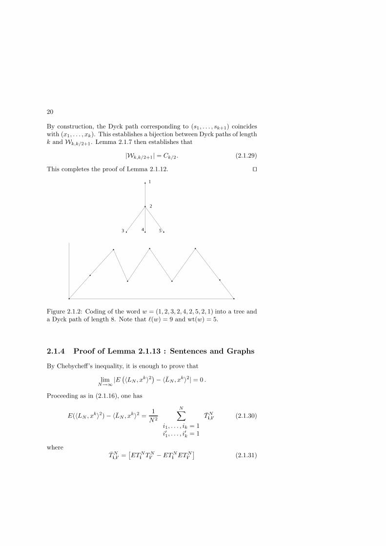
determines a path v1, v2, . . . , vk, vk+1 = v1 of length k + 1 on the tree Gw.We refer to this path as the exploration process associated with w. Letd(v, v′) denotes the distance between vertices v, v′ on the tree Gw, i.e. theshortest path on the tree beginning at v and terminating at v′. Settingxi = d(vi+1, v1), one sees that each word w ∈ Wk,k/2+1 defines a Dyck pathx1, x2, . . . , xk = 0 of length k. Conversly, given a Dyck path x1, . . . , xk,one may construct a word w ∈ Wk,k/2+1 by recursively constructing anincreasing (with respect to inclusion) sequence of trees Ti, i = 1, 2, . . . , k+1,and an exploration process vi, i = 1, . . . , k+1, on Tk+1, as follows. The treeT1 consists of a single vertex v labelled 1, and we set v1 = v. Given a treeTi with vertices labelled 1, 2, . . . , ji, and a vertex vi ∈ Ti, if xi+1 = xi + 1then Ti+1 consists of the tree Ti augmented with a new vertex v labelledji + 1, and we set vi+1 = v. If xi+1 = xi − 1, then Ti+1 = Ti but vi+1 isthe ancestor of vi in Ti. Taking w = (s1, s2, . . . , sk+1) to be the sequence oflabels attached to the sequence {vi}, one obtains an element of Wk,k/2+1.
20
By construction, the Dyck path corresponding to (s1, . . . , sk+1) coincideswith (x1, . . . , xk). This establishes a bijection between Dyck paths of lengthk and Wk,k/2+1. Lemma 2.1.7 then establishes that
|Wk,k/2+1| = Ck/2. (2.1.29)
This completes the proof of Lemma 2.1.12. ut1
2
3 4 5
Figure 2.1.2: Coding of the word w = (1, 2, 3, 2, 4, 2, 5, 2, 1) into a tree anda Dyck path of length 8. Note that `(w) = 9 and wt(w) = 5.
2.1.4 Proof of Lemma 2.1.13 : Sentences and Graphs
By Chebycheff’s inequality, it is enough to prove that
limN→∞
|E(〈LN , x
k〉2)− 〈LN , x
k〉2| = 0 .
Proceeding as in (2.1.16), one has
E(〈LN , xk〉2) − 〈LN , x
k〉2 =1
N2
N∑
i1, . . . , ik = 1i′1, . . . , i
′k = 1
TNi,i′ (2.1.30)
whereTNi,i′ =
[ETN
i TNi′ − ETN
i ETNi′]
(2.1.31)
21
The role of words in the proof of Lemma 2.1.12 is now played by pairs ofwords, which is a particular case of a sentence.
Definition 2.1.32 (S-Sentences) Given a set S, an S-sentence a is afinite sequence of S-words w1, . . . , wn, at least one word long. Two S-sentences a1, a2 are called equivalent, denoted a1 ∼ a2, if there is a bijectionon S that maps one into the other.
As with words, for a sentence a = (w1, w2, . . . , wn), we define the supportas supp (a) = ∪n
i=1supp (wi), and its weight wt(a) as the cardinality ofsupp (a).
Definition 2.1.33 (Graph associated to an S-sentence) Given a sen-tence a = (w1, . . . , wk), with wi = (si
1, si2, . . . , s
i`(wi)
), we set Ga = (Va, Ea)
to be the graph with set of vertices Va = supp (a) and (undirected) edges
Ea = {{sij, s
ij+1}, j = 1, . . . , `(wi) − 1, i = 1, . . . , k}.
We define the set of self edges as Esa = {e ∈ Ea : e = {u, u}, u ∈ Va} and
the set of connecting edges as Eca = Ea \ Es
a.
In words, the graph associated with a sentence a = (w1, . . . , wk) is obtainedby piecing together the graphs of the individual words wi (and in general, itdiffers from the graph associated with the word obtained by concatenatingthe words wi!). Unlike the graph of a word, the graph associated with asentence may be disconnected. Note that the sentence a defines k paths inthe graph Ga. For e ∈ Ea, we use Na
e to denote the number of times theunion of these paths traverses the edge e (in any direction). We note thatequivalent sentences generate the same graphs Ga and the same passagecounts Na
e .
Coming back to the evaluation of Ti,i′ , see (2.1.30), recall the closed wordswi, wi′ of length k + 1, and define the two-words sentence ai,i′ = (wi, wi′).Then,
TNi,i′ =
1
Nk
[ ∏
e∈Ecai,i′
E(ZNa
e1,2 )
∏
e∈Esai,i′
E(YNa
e1 ) (2.1.34)
−∏
e∈Ecwi
E(ZNwi
e1,2 )
∏
e∈Eswi
E(Y Nwi
e1 )
∏
e∈Ecwi′
E(ZNwi′
e1,2 )
∏
e∈Eswi′
E(Y Nwi′
e1 )
].
In particular, TNi,i′ = 0 unless N
ai,i′
e ≥ 2 for all e ∈ Eai,i′ . Also, TN
i,i′ = 0unless Ewi
∩ Ewi′ 6= ∅. Further, (2.1.34) shows that if ai,i′ ∼ aj,j′ then

22
TNi,i′ = TN
j,j′ . Finally, if N ≥ t then there are exactly CN,t N -sentences thatare equivalent to a given N -sentence of weight t. We set, with N > t,
W(2)k,t denotes the equivalent classes of sentences a of weight t
consisting of two closed words (w1, w2), each of length k + 1,with Na
e ≥ 2 for each e ∈ Ea, and Ew1 ∩ Ew2 6= ∅ .
(2.1.35)
One deduces from (2.1.30) and (2.1.34) that
E(〈LN , xk〉2) − 〈LN , x
k〉2 (2.1.36)
=
2k∑
t=1
CN,t
Nk+2
∑
a=(w1,w2)∈W(2)k,t
[ ∏
e∈Eca
E(ZNa
e1,2 )
∏
e∈Esa
E(YNa
e1 )
−∏
e∈Ecw1
E(ZNw1
e1,2 )
∏
e∈Esw1
E(YNw1
e1 )
∏
e∈Ecw2
E(ZNw2
e1,2 )
∏
e∈Esw2
E(YNw2
e1 )
],
where the sum is over a set of representatives, belonging to W(2)k,t , of equiv-
alent classes of sentences. We have completed the preliminaries to:
Proof of Lemma 2.1.13 In view of (2.1.36), since W(2)k,t does not depend
on N for N ≥ t, it suffices to check that W(2)k,t is empty for t ≥ k+ 2. Since
we need it later, we prove a slightly stronger claim, namely that W(2)k,t is
empty for t ≥ k + 1.
Toward this end, note that if a ∈ W(2)k,t then Ga is a connected graph,
with t vertices and at most k edges (since Nae ≥ 2 for e ∈ Ea), which is
impossible when t > k + 1. Considering the case t = k + 1, it follows thatGa is a tree, and each edge must be visited by the paths generated by aexactly twice. Because the path generated by w1 in the tree Ga starts andend at the same vertex, it must visit each edge an even number of times.Thus, the set of edges visited by w1 is disjoint from the set of edges visited
by w2, contradicting the definition of W(2)k,t . ut
Remark 2.1.37 Note that in the course of the proof of Lemma 2.1.13, weactually showed that for N > 2k,
E(〈LN , xk〉2) − 〈LN , x
k〉2 (2.1.38)
=
k∑
t=1
CN,t
Nk+2
∑
a=(w1,w2)∈W(2)k,t
[ ∏
e∈Eca
E(ZNa
e1,2 )
∏
e∈Esa
E(YNa
e1 )
−∏
e∈Ecw1
E(ZNw1
e1,2 )
∏
e∈Esw1
E(YNw1
e1 )
∏
e∈Ecw2
E(ZNw2
e1,2 )
∏
e∈Esw2
E(YNw2
e1 )
].

23
Exercise 2.1.39 Check that Theorem 2.1.4 still holds for symmetric randommatricesXN if the zero mean independent random variables {XN(i, j)}1≤i≤j≤N
are not assumed identically distributed, but rather one assumes that for allε > 0,
limN→∞
#{(i, j) : |1 −NEXN(i, j)2| < ε}N2
= 1 ,
and for all k ≥ 1, there exists a finite rk independent of N such that
sup1≤i≤j≤N
E∣∣∣√NXN(i, j)
∣∣∣k
≤ rk .
Exercise 2.1.40 Check that the conclusion of Theorem 2.1.4 remains truewhen convergence in probability is replaced by almost sure convergence.Hint: Using Chebycheff’s inequality and the Borel-Cantelli lemma, it is enoughto verify that for all integer k, there exists a constant C = C(k) such that
|E(〈LN , x
k〉2)− 〈LN , x
k〉2| ≤ C
N2.
Exercise 2.1.41 We develop in this exercise the limit theory for Wishart ma-trices. LetM = M(N) be a sequence of integers such that limN→∞M(N)/N =α ∈ [1,∞) . Consider an N ×M(N) matrix YN with i.i.d. entries of meanzero and variance 1/N , and such that E
(Nk/2|YN (1, 1)|k
)≤ rk <∞ . Define
the N ×N Wishart matrix as WN = YNY∗N , and let LN denote the empirical
measure of the eigenvalues of WN . Set LN = ELN .(i) Write N〈LN , x
k〉 as
∑
i1, . . . , ikj1, . . . , jk
EYN (i1, j1)YN (i2, j1)YN (i2, j2)YN (i3, j2) · · ·YN (ik, jk)YN (i1, jk)
and show that the only contributions to the sum that survive the passage tothe limit are those in which each term appears exactly twice.(ii) Code the contributions as Dyck paths, where the even heights correspondto i indices and the odd heights correspond to j indices. Let ` = `(i, j) denotethe number of times the excursion makes a descent from an odd height to aneven height (this is the number of distinct j indices in the tuple!), and showthat the combinatorial weight of such a path is asymptotic to Nk+1α`.(iii) Let ¯ denote the number of times the excursion makes a descent from aneven height to an odd height, and set
βk =∑
Dyck paths of length 2k
α` , γk =∑
Dyck paths of length 2k
α¯.
24
(The βk are the k-th moments of any weak limit of LN .) Prove that
βk = α
k∑
j=1
γk−jβj−1 , γk =
k∑
j=1
βk−jγj−1 , k ≥ 1 .
(iv) Setting βα(z) =∑∞
k=0 zkβk, prove that βα(z) = 1 + zβα(z)2 + (α −
1)zβα(z), and thus the limit Fα of LN possesses the Stieltjes transform
−z−1βα(1/z), where
βα(z) =
1 − (α− 1)z −√
1 − 4z[
α+12 − (α−1)2z
4
]
2z.
(v) Conclude that Fα possesses a density fα supported on [b−, b+], with b− =(1 −√
α)2/α, b+ = (1 +√α)2/α, satisfying
fα(x) =α√
(x− b−)(b+ − x)
2πx, x ∈ [b−, b+] . (2.1.42)
(vi) Prove the analog of Lemma 2.1.13 for Wishart matrices, and deduce thatLN → Fα weakly, in probability.(vii) Note that F1 is the image of the semi-circle distribution under the trans-formation x 7→ x2.
2.1.5 Some useful approximations
This section is devoted to the following simple observation, that often al-lows one to considerably simplify arguments concerning the convergence ofempirical measures.
Lemma 2.1.43 Let A, B be N ×N symmetric matrices, with eigenvaluesλA
1 ≤ λA2 ≤ . . . ≤ λA
N and λB1 ≤ λB
2 ≤ . . . ≤ λBN . Then,
N∑
i=1
|λAi − λB
i |2 ≤ Tr(A−B)2 .
Proof: Note that TrA2 =∑
i(λAi )2 and TrB2 =
∑i(λ
Bi )2. Let U de-
note the matrix diagonalizing B written in the basis determined by A, andlet DA, DB denote the diagonal matrices with diagonal elements λA
i , λBi
respectively. Then,
TrAB = TrDAUDBUT =
∑
i,j
λAi λ
Bj u
2ij .
25
The last sum is linear in the coefficients vij = u2ij , and the orthogonality of
U implies that∑
j vij = 1,∑
i vij = 1. Thus,
TrAB ≤ supvij≥0:
Pj vij=1,
Pi vij=1
∑
i,j
λAi λ
Bj vij . (2.1.44)
But this is a maximization of a linear functional over the set of doublystochastic matrices, and the maximum is obtained at the extreme points,which are well known to correspond to permutations4. The maximumamong permutations is then easily checked to be
∑i λ
Ai λ
Bi . Collecting these
facts together implies Lemma 2.1.43. Alternatively5, one sees directly thata maximizing V = {vij} in (2.1.44), is the identity matrix. Indeed, as-sume w.l.o.g. that v11 < 1. We then construct a matrix V = {vij} withv11 = 1 and vii = vii for i > 1 such that V is also a maximizing matrix.Indeed, because v11 < 1, there exist a j and a k with v1j > 0 and vk1 > 0.Set v = min(v1j , vk1) > 0 and define v11 = v11 + v, vkj = vkj + v andv1j = v1j − v, vk1 = vk1 − v, and vab = vab for all other pairs ab. Then,
∑
i,j
λAi λ
Bj (vij − vij) = v(λA
1 λB1 + λA
k λBj − λA
k λB1 − λA
1 λBj )
= v(λA1 − λA
k )(λB1 − λB
j ) ≥ 0 .
Thus, V = {vij} satisfies the constraints, is also a maximum, and thenumber of zero elements in the first row and column of V is larger by 1 atleast from the corresponding one for V . If v11 = 1, the claims follows, whileif v11 < 1, one repeats this (at most 2N −2 times) to conclude. Proceedingin this manner with all diagonal elements of V , one sees that indeed themaximum of the right hand side of (2.1.44) is
∑i λ
Ai λ
Bi , as claimed. ut
Remark 2.1.45 One notes that the statement and proof of Lemma 2.1.43carry over to the case where A and B are both Hermitian matrices.
Lemma 2.1.43 allows one to perform all sorts of truncations when prov-ing convergence of empirical measures. For example, let us prove the fol-lowing variant of Wigner’s Theorem 2.1.4.
Theorem 2.1.46 AssumeXN is as in (2.1.2), except that instead of (2.1.1),only r2 <∞ is assumed. Then, the conclusion of Theorem 2.1.4 still holds.
4This theorem is usually attributed to G. Birkhoff. See [Chv83] for a proof and ahistorical discussion which attributes this result to D. Konig.
5Thanks to Hongjie Dong for pointing this out.
26
Proof: Fix a constant C and consider the matrix XN whose elementssatisfy, for i ≤ j and i = 1, . . . , N ,
XN (i, j) = XN (i, j)1√N |XN (i,j)|≤C − E(XN (i, j)1√
N |XN (i,j)|≤C).
Then, with λNi denoting the eigenvalues of XN , ordered, it follows from
Lemma 2.1.43 that
1
N
N∑
i=1
|λNi − λN
i |2 ≤ 1
NTr(XN − XN )2 .
But,
WN :=1
NTr(XN − XN )2
≤ 1
N2
∑
i,j
[√NXN (i, j)1|
√NXN (i,j)|≥C − E(
√NXN (i, j)1|
√NXN (i,j)|≥C)
]2.
Since r2 < ∞, and the involved random variables are identical in law toeither Z1,2 or Y1, it follows that E[(
√NXN (i, j))21|
√NXN (i,j)|≥C ] converges
to 0 uniformly inN, i, j, when C converges to infinity. Hence, one may chosefor each ε a C large such that P (|WN | > ε) < ε. Further, let
Lip(R) = {f ∈ Cb(R) : supx
|f(x)| ≤ 1, supx 6=y
|f(x) − f(y)
|x− y| ≤ 1} .
Then, on the event {|WN | < ε}, it holds that for f ∈ Lip(R),
|〈LN , f〉 − 〈LN , f〉| ≤1
N
∑
i
|λNi − λN
i | ≤ √ε ,
where LN denotes the empirical measure of the eigenvalues of XN , andJensen’s inequality was used in the second inequality. This, together withthe weak convergence in probability of LN toward the semicircle law assuredby Theorem 2.1.4, and the fact that weak convergence is equivalent toconvergence with respect to the Lipschitz bounded metric, see TheoremC.8, complete the proof of Theorem 2.1.46. ut
2.1.6 Maximal eigenvalues and Furedi-Komlos enumer-ation
Wigner’s theorem asserts the weak convergence of the empirical measure ofeigenvalues to the compactly supported semi-circle law. One immediately

27
is led to suspect that the maximal eigevalue of XN should converge to thevalue 2, the largest element of the support of the semi-circle distribution.This fact, however, does not follow from Wigner’s theorem. However, thecombinatorial techniques we already saw allow one to prove the following,where we use the notation introduced in (2.1.1) and (2.1.2).
Theorem 2.1.47 (Maximal eigenvalue) Consider a Wigner matrix XN
satisfying rk ≤ kCk for some constant C and all integer k. Then, λNN con-
verges to 2 in probability.
Remark: The assumption of Theorem 2.1.47 holds if the random variables|Z1,2| and |Y1| possess a finite exponential moment.
Proof of Theorem 2.1.47 Fix δ > 0 and let g : R 7→ R+ be a continuousfunction supported on [2 − δ, 2], with 〈g, σ〉 = 1. Then, applying Wigner’stheorem 2.1.4,
P (λNN < 2 − δ) ≤ P (〈LN , g〉 = 0) ≤ P (|〈LN , g〉 − 〈σ, g〉| > 1
2) →N→∞ 0 .
(2.1.48)We thus need to provide a complimentary estimate on the probability thatλN
N is large. We do that by estimating 〈LN , x2k〉 for N -dependent k, using
the bounds on rk provided in the assumptions. The key step is containedin the following combinatorial lemma, that gives information on the setsWk,t, see (2.1.24).
Lemma 2.1.49 For all integers k > 2t−2 and N > t one has the estimate
|Wk,t| ≤ 2kk3(k−2t+2) . (2.1.50)
The proof of Lemma 2.1.49 is deferred to the end of this section.
Equipped with Lemma 2.1.49, we have for 2k < N , using (2.1.25),
〈LN , x2k〉 (2.1.51)
≤k+1∑
t=1
N t−(k+1)|W2k,t| supw∈W2k,t
∏
e∈Ecw
E(ZNw
e1,2 )
∏
e∈Esw
E(YNw
e1 )
≤ 4kk+1∑
t=1
[(2k)6
N
]k+1−t
supw∈W2k,t
∏
e∈Ecw
E(ZNw
e1,2 )
∏
e∈Esw
E(YNw
e1 ) .
To evaluate the last expectation, fix w ∈ W2k,t, and let l denote the numberof edges in Ec
w with Nwe = 2. Holder’s inequality then gives
∏
e∈Ecw
E(ZNw
e1,2 )
∏
e∈Esw
E(YNw
e1 ) ≤ r2k−2l ,
28
with the convention that r0 = 1. Since Gw is connected, |Ecw| ≥ |Vw | − 1 =
t − 1. On the other hand, by noting that Nwe ≥ 3 for |Ec
w| − l edges, onehas 2k ≥ 3(|Ec
w| − l) + 2l+ 2|Esw|. Hence, 2k− 2l ≤ 6(k + 1− t). Since r2q
is a non-decreasing function of q bounded below by 1, we get, substitutingback in (2.1.51), that for some constant c1 = c1(C) and all k < N ,
〈LN , x2k〉 ≤ 4k
k+1∑
t=1
[(2k)6
N
]k+1−t
r6(k+1−t)
≤ 4kk+1∑
t=1
[(2k)6(6(k + 1 − t))6C
N
]k+1−t
≤ 4kk∑
i=0
[kc1
N
]i
. (2.1.52)
Choose next a sequence k(N) →N→∞ ∞ such that k(N)c1/N →N→∞ 0but k(N)/ logN →N→∞ ∞. Then, for any δ > 0, and all N large,
P (λNN > (2 + δ)) ≤ P (N〈LN , x
2k(N)〉 > (2 + δ)2k(N))
≤ N〈LN , x2k(N)〉
(2 + δ)2k(N)
≤ 2N4k(N)
(2 + δ)2k(N)→N→∞ 0 ,
completing the proof of Theorem 2.1.47. utProof of Lemma 2.1.49 The idea of the proof it to keep track of thenumber of possibilities to prevent words in Wk,t from having weight bk/2c+1. Toward this end, let w ∈ Wk,t be given. A parsing of the word w is asentence aw = (w1, . . . , wn) such that the word obtained by concatenatingthe words wi is w. One can imagine creating a parsing of w by introducingcommas between parts of w.
We say that a parsing a = aw ofw is an FK parsing, and call the sentencea an FK sentence, if the graph associated with a is a tree, if Na
e ≤ 2 forall e ∈ Ea, and if for any i = 1, . . . , n − 1, the first letter of wi+1 belongsto ∪i
j=1suppwj . If the one word sentence a = w is an FK parsing, we saythat w is an FK word. Note that the constituent words in an FK parsingare FK words.
As will become clear next, the graph of an FK word consists of treeswhose edges have been visited twice by w, glued together by edges thathave been visited only once. Recalling that a Wigner word is either a oneletter word or a closed word of odd length and maximal weight, this leadsto the following lemma.

29
Lemma 2.1.53 Each FK word can be written in a unique way as a con-catenation of pairwise disjoint Wigner words. Further, there are at most2n−1 equivalence classes of FK words of length n.
Proof of Lemma 2.1.53 Let w = (s1, . . . , sn) be an FK word of length n.By definition, Gw is a tree. Let {sij , sij+1}r
j=1 denote those edges of Gw
visited only once by the walk induced by w. Defining i0 = 1, one sees thatthe words wj = (sij−1 , . . . , sij−1), j ≥ 1, are closed, disjoint, and visit eachedge in the tree Gwj exactly twice. In particular, with lj := ij − ij−1 − 1,it holds that lj is even (possibly, lj = 0 if wj is a one letter word), andfurther if lj > 0 then wj ∈ Wlj ,lj/2+1. This decomposition being unique,one concludes that for any z, with Nn denote the number of equivalenceclasses of FK words of length n, and with |W0,1| := 1,
∞∑
n=1
Nnzn =
∞∑
r=1
∑
{lj}rj=1
lj even
r∏
j=1
zlj+1|Wlj ,lj/2+1|
=
∞∑
r=1
(z +
∞∑
l=1
z2l+1|W2l,l+1|)r
, (2.1.54)
in the sense of formal power series. By the proof of Lemma 2.1.12, |W2l,l+1| =Cl = βl. Hence, by Lemma 2.1.7, for |z| < 1/4,
z +∞∑
l=1
z2l+1|W2l,l+1| = zβ(z2) =1 −
√1 − 4z2
2z.
Substituting in (2.1.54), one sees that (again, in the sense of power series)
∞∑
n=1
Nnzn =
zβ(z2)
1 − zβ(z2)=
1 −√
1 − 4z2
2z − 1 +√
1 − 4z2= −1
2+
z + 12√
1 − 4z2.
Using that √1
1 − t=
∞∑
k=0
tk
4k
(2kk
),
one concludes that
∞∑
n=1
Nnzn = z +
1
2(1 + 2z)
∞∑
n=1
z2n
(2nn
),
from which Lemma 2.1.53 follows. utOur interest in FK parsings is the following FK parsing w′ of a word
w = (s1, . . . , sn). Declare an edge e of Gw to be new (relative to w) if for
30
some index 1 ≤ i < n we have e = {si, si+1} and si+1 6∈ {s1, . . . , si}. If theedge e is not new, then it is old. Define w′ to be the sentence obtained bybreaking w (that is, “inserting a comma”) at all visits to old edges of Gw
and at third and subsequent visits to new edges of Gw.
1
2 3
4
56
7
1
2 3
4
5
7
6
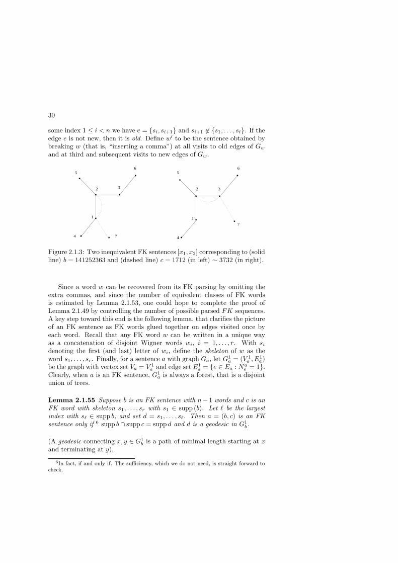
Figure 2.1.3: Two inequivalent FK sentences [x1, x2] corresponding to (solidline) b = 141252363 and (dashed line) c = 1712 (in left) ∼ 3732 (in right).
Since a word w can be recovered from its FK parsing by omitting theextra commas, and since the number of equivalent classes of FK wordsis estimated by Lemma 2.1.53, one could hope to complete the proof ofLemma 2.1.49 by controlling the number of possible parsed FK sequences.A key step toward this end is the following lemma, that clarifies the pictureof an FK sentence as FK words glued together on edges visited once byeach word. Recall that any FK word w can be written in a unique wayas a concatenation of disjoint Wigner words wi, i = 1, . . . , r. With si
denoting the first (and last) letter of wi, define the skeleton of w as theword s1, . . . , sr. Finally, for a sentence a with graph Ga, let G1
a = (V 1a , E
1a)
be the graph with vertex set Va = V 1a and edge set E1
a = {e ∈ Ea : Nae = 1}.
Clearly, when a is an FK sentence, G1a is always a forest, that is a disjoint
union of trees.
Lemma 2.1.55 Suppose b is an FK sentence with n− 1 words and c is anFK word with skeleton s1, . . . , sr with s1 ∈ supp (b). Let ` be the largestindex with s` ∈ supp b, and set d = s1, . . . , s`. Then a = (b, c) is an FKsentence only if 6 supp b ∩ supp c = supp d and d is a geodesic in G1
b .
(A geodesic connecting x, y ∈ G1b is a path of minimal length starting at x
and terminating at y).
6In fact, if and only if. The sufficiency, which we do not need, is straight forward tocheck.
31
Before providing the proof of Lemma 2.1.55, we explain how it leads totheCompletion of proof of Lemma 2.1.49 Let Γ(t, `,m) denote the setof equivalence classes of FK sentences a = (w1, . . . , wm) consisting of mwords, with total length
∑mi=1 `(wi) = ` and wt(a) = t. An immediate
corrolary of Lemma 2.1.55 is that
|Γ(t, `,m)| ≤ 2`−mt2(m−1)
(`− 1m− 1
). (2.1.56)
Indeed, there are c`,m :=
(`− 1m− 1
)m-tuples of integers summing to `,
and thus at most 2`−mc`,m equivalence classes of m FK words with sum oflengths equal to `. Lemma 2.1.55 then shows that there are at most t2(m−1)
ways to “glue these words into an FK sentence”, whence (2.1.56) follows.
For any FK sentence a consisting of m words with total length `, wehave that
m = |E1a | − 2wt(a) + 2 + ` . (2.1.57)
Indeed, the word obtained by concatenating the words of a generates a listof (not necessarily distinct) `−1 unordered pairs of adjoining letters, out ofwhich m− 1 correspond to commas in the FK sentence a and 2|Ea| − |E1
a|correspond to edges of Ga. Using that |Ea| = |Va|−1, (2.1.57) follows. Butthen, any word w ∈ Wk,t can be parsed into an FK sentence w′ consistingof m words. Note that if an edge e is retained in Gw′ , then no comma isinserted at e at the first and second passage on e (but is introduced if thereare further passages on e). Therefore, E1
w′ = ∅. By (2.1.57), this impliesthat for such words, m− 1 = k+ 2− 2t. Equation (2.1.56) then allows oneto conclude the proof of Lemma 2.1.49. utProof of Lemma 2.1.55 Assume a is an FK sentence. Then, Ga is atree, and since the Wigner words composing c are disjoint, d is the uniquegeodesic in Gc ⊂ Ga connecting s1 to s`. Hence, it is also the uniquegeodesic in Gb ⊂ Ga connecting s1 to s`. But d visits only edges of Gb thathave been visited exactly once by the constituent words of b, for otherwise(b, c) would not be an FK sentence (that is, a comma would need to beinserted to split c). Thus, Ed ⊂ E1
b . Since c is an FK word, E1c = E(s1,...,sr).
Since a is an FK sentence, Eb ∩ Ec = E1b ∩ E1
c . Thus, Eb ∩ Ec = Ed. But,recall that Ga, Gb, Gc, Gd are trees, and hence
|Va| = 1 + |Ea| = 1 + |Eb| + |Ec| − |Eb ∩ Ec| = 1 + |Eb| + |Ec| − |Ed|= 1 + |Eb| + 1 + |Ec| − 1 − |Ed| = |Vb| + |Vc| − |Vd| .
Since |Vb| + |Vc| − |Vb ∩ Vc| = |Va|, it follows that |Vd| = |Vb ∩ Vc|. SinceVd ⊂ Vb ∩ Vc, one concludes that Vd = Vb ∩ Vc, as claimed. ut

32
Remark 2.1.58 The result described in Theorem 2.1.47 is not optimal,in the sense that even with uniform bounds on the (rescaled) entries, i.e.rk uniformly bounded, the estimate one gets on the displacement of themaximal eigenvalue to the right of 2 is O(n−1/6 logn), whereas the truedisplacement is known to be of order n−1/6 ([TW96], [Sos99]). For moreon that in the context of complex Gaussian Wigner matrices, see Theorem3.1.10.
Exercise 2.1.59 Prove that the conclusion of Theorem 2.1.47 holds withconvergence in probability replaced by either almost sure convergence or Lp
convergence.
Exercise 2.1.60 Prove that the statement of Theorem 2.1.47 can be strength-ened to yield that for some constant δ = δ(C) > 0, N δ(λN
N − 2) converges to0, almost surely.
Exercise 2.1.61 Assume that for some constants λ > 0, C, the independent(but not necessarily identically distributed) entries {XN(i, j)}1≤i≤j≤N of thesymmetric matrices XN satisfy
supi,j,N
E(eλ√
N |XN (i,j)|) ≤ C .
Prove that there exists a constant c1 = c1(C) such that lim supN→∞ λNN ≤ c1,
almost surely, and lim supN→∞EλNN ≤ c1.
Exercise 2.1.62 We develop in this exercise an alternative proof, that avoidsmoment computations, to the conclusion of Exercise 2.1.61, under the strongerassumption that for some λ > 0,
supi,j,N
E(eλ(√
N |XN (i,j)|)2 ) ≤ C .
a) Prove (using Chebycheff’s inequality and the assumption) that there existsa constant c0 independent of N such that for any fixed z ∈ RN , and all Clarge enough,
P (‖zTXN‖2 > C) ≤ e−c0C2N . (2.1.63)
b) Let Nδ = {zi}Nδ
i=1 be a minimal deterministic net in the unit ball of RN ,that is ‖zi‖2 = 1, supz:‖z‖2=1 infi ‖z−zi‖2 ≤ δ, and Nδ is the minimal integerwith the property that such a net can be found. Check that
(1 − δ2) supz:‖z‖2=1
zTXNz ≤ supzi∈Nδ
zTi XNzi + 2 sup
isup
z:‖z−zi‖2≤δ
zTXNzi .
(2.1.64)c) Combine steps a) and b) and the estimate Nδ ≤ cNδ , valid for some cδ > 0,to conclude that there exists a constant c2 independent of N such that for allC large enough, independently of N ,
P (λNN > C) = P ( sup
z:‖z‖2=1
zTXNz > C) ≤ e−c2C2N .
33
2.1.7 Central limit theorems for moments
Our goal here is to derive a simple version of a central limit theorem (CLT)for linear statistics of the eigenvalues of Wigner matrices. With XN aWigner matrix and LN the associated empirical measure of its eigenvalues,set ZN,k := N [〈LN , x
k〉 − 〈LN , xk〉]. Let
Φ(x) =1√2π
∫ x
−∞e−u2/2du
denote the Gaussian distribution. We set σ2k as in (2.1.75) below, and prove
the following.
Theorem 2.1.65 The law of the sequence of random variables ZN,k/σk
converges weakly to the standard Gaussian distribution. More precisely,
limN→∞
P
(ZN,k
σk≤ x
)= Φ(x) . (2.1.66)
Proof of Theorem 2.1.65 Most of the proof consists of a variance compu-tation. The reader interested only in a proof of convergence to a Gaussiandistribution (without worrying about the actual variance) can skip to thetext following equation (2.1.75).
Recall the notation W(2)k,t introduced in the course of proving Lemma 2.1.13.
Using (2.1.38), we have
limN→∞
E(Z2N,k) (2.1.67)
= limN→∞
N2[E(〈LN , x
k〉2) − 〈LN , xk〉2]
=∑
a=(w1,w2)∈W(2)k,k
[ ∏
e∈Eca
E(ZNa
e1,2 )
∏
e∈Esa
E(YNa
e1 )
−∏
e∈Ecw1
E(ZNw1
e1,2 )
∏
e∈Esw1
E(YNw1
e1 )
∏
e∈Ecw2
E(ZNw2
e1,2 )
∏
e∈Esw2
E(YNw2
e1 )
].
We note next that if a = (w1, w2) ∈ W(2)k,k then Ga is connected and pos-
sesses k vertices and at most k edges, each visited at least twice by thepaths generated by a. Hence, with k vertices, Ga possesses either k − 1 or
k edges. Let W(2)k,k,+ denote the subset of W(2)
k,k such that |Ea| = k (that is,Ga is unicyclic, i.e. “possesses one edge too much to be a tree”) and let
W(2)k,k,− denote the subset of W(2)
k,k such that |Ea| = k − 1.
Suppose first a ∈ W(2)k,k,−. Then, Ga is a tree, Es
a = ∅, and necessarilyGwi is a subtree of Ga. This implies that k is even and that |Ewi | ≤ k/2.

34
In this case, for Ew1 ∩ Ew2 6= ∅ one must have |Ewi | = k/2, which impliesthat all edges of Gwi are visited twice by the walk generated by wi, andexactly one edge is visited twice by both w1 and w2. In particular, wi areboth closed Wigner words of length k + 1. The emerging picture is of twotrees with k/2 edges each “glued together” at one edge. Since there areCk/2 ways to chose each of the trees, k/2 ways of choosing (in each tree)the edge to be glued together, and 2 possible orientations for the glueing,we deduce that
|W(2)k,k,−| = 2
(k
2
)2
C2k/2 . (2.1.68)
Further, for each a ∈ W(2)k,k,−,
[ ∏
e∈Eca
E(ZNa
e1,2 )
∏
e∈Esa
E(YNa
e1 )
−∏
e∈Ecw1
E(ZNw1
e1,2 )
∏
e∈Esw1
E(YNw1
e1 )
∏
e∈Ecw2
E(ZNw2
e1,2 )
∏
e∈Esw2
E(YNw2
e1 )
]
= E(Z41,2)[E(Z2
1,2)]k−2 − [E(Z2
1,2)]k
= E(Z41,2) − 1 . (2.1.69)
We next turn to consider W(2)k,k,+. In order to do so, we need to understand
the structure of unicyclic graphs.
Definition 2.1.70 A graph G = (V,E) is called bracelet if there exists anenumeration α1, α2, . . . , αr of V such that
E =
{{α1, α1}} if r = 1,{{α1, α2}} if r = 2,
{{α1, α2}, {α2, α3}, {α3, α1}} if r = 3,{{α1, α2}, {α2, α3}, {α3, α4}, {α4, α1}} if r = 4,
and so on. We call r the circuit length of the bracelet G.
We need the following elementary lemma, allowing one to decompose aunicyclic graph as a bracelet and its associated pendant trees. Recall thata graph G = (V,E) is unicyclic if it is connected and |E| = |V |.
Lemma 2.1.71 Let G = (V,E) be a unicyclic graph. Let Z be the subgraphof G consisting of all e ∈ E such that G \ e is connected, along with allattached vertices. Let r be the number of edges of Z. Let F be the graphobtained from G by deleting all edges of Z. Then, Z is a bracelet of circuitlength r, F is a forest with exactly r connected components, and Z meetseach connected component of F in exactly one vertex. Further, r = 1 ifEs 6= ∅ while r ≥ 3 otherwise.

35
We call Z the bracelet of G. We call r the circuit length of G, and each ofthe components of F we call a pendant tree.
23
4
5
67
8
1
Figure 2.1.4: The bracelet 1234 of circuit length 4, and the pen-dant trees, associated with the unicyclic graph corresponding to[12565752341, 2383412]
Coming back to a ∈ W(2)k,k,+, let Za be the associated bracelet (with
circuit length r = 1 or r ≥ 3). Note that for any e ∈ Ea one has Nae = 2.
We claim next that e ∈ Za if an only if Nw1e = Nw2
e = 1: indeed, if e ∈ Za
then (Va, Ea \ e) is a tree. If one of the paths determined by w1 and w2 failto visit e then all edges visited by this path determine a walk on a tree andtherefore the path visits each edge exactly twice. This then implies thatthe set of edges visited by the walks are disjoint, a contradiction. On theother hand, if e = (x, y) and Nwi
e = 1 then all vertices in Vwi are connectedto x and to y by a path using only edges from Ewi \ e. Hence, (Va, Ea \ e)is connected, and thus e ∈ Za.
Thus, any a = (w1, w2) ∈ W(2)k,k,+ with bracelet length r can be con-
structed from the following data: the pendant trees {T ij}r
j=1 (possiblyempty) associated to each word wi and each vertex j of the bracelet Za, thestarting point for each word wi on the graph consisting of the bracelet Za
and trees {T ij}, and whether Za is traversed by the words wi in the same
or in opposing directions (in case r ≥ 3). In view of the above, countingthe number of ways to attach trees to a bracelet of length r, and then thedistinct number of non-equivalent ways to choose starting points for thepaths on the resulting graph, there are exactly
21r≥3k2
r
∑
ki≥0:
2Pr
i=1 ki=k−r
r∏
i=1
Cki
2
(2.1.72)

36
elements of W(2)k,k,+ with bracelet of length r. Further, for a ∈ W(2)
k,k,+ wehave
[ ∏
e∈Eca
E(ZNa
e1,2 )
∏
e∈Esa
E(YNa
e1 )
−∏
e∈Ecw1
E(ZNw1
e1,2 )
∏
e∈Esw1
E(YNw1
e1 )
∏
e∈Ecw2
E(ZNw2
e1,2 )
∏
e∈Esw2
E(YNw2
e1 )
]
=
{(E(Z2
1,2))k − 0 if r ≥ 3
(E(Z21,2))
k−1EY 21 − 0 if r = 1
=
{1 if r ≥ 3EY 2
1 if r = 1(2.1.73)
Combining (2.1.67), (2.1.68), (2.1.69), (2.1.72) and (2.1.73), and settingCx = 0 if x is not an integer, one obtains, with
σ2k = k2C2
k−12
EY 21 +
k2
2C2
k2[EZ4
1,2 − 1] +
∞∑
r=3
2k2
r
∑
ki≥0:
2P
ri=1 ki=k−r
r∏
i=1
Cki
2
,
(2.1.74)that
σ2k = lim
N→∞EZ2
N,k . (2.1.75)
The rest of the proof consists in verifying that, for j ≥ 3,
limN→∞
E
(ZN,k
σk
)j
=
{0 , j is odd,(j − 1)!! , j is even .
(2.1.76)
where (j − 1)!! = (j − 1)(j − 3) · · · 1. Indeed, this completes the proofof the theorem since the right hand side of (2.1.76) coincides with themoments of the Gaussian distribution Φ, and the latter moments determinethe Gaussian distribution by an application of Carleman’s theorem (see,e.g., [Dur96]), since
∑∞n=1[(2j − 1)!!](−1/2j) = ∞.
To see (2.1.76), recall, for a multi-index i = (i1, . . . , ik), the terms TNi
of (2.1.23), and the associated closed word wi. Then, as in (2.1.30), onehas
E(ZjN,k) =
N∑
in1 , . . . , ink = 1
n = 1, 2, . . . j
TNi1,i2,...,ij (2.1.77)
where
TNi1,i2,...,ij = E
[j∏
n=1
(TNin − ETN
in )
]. (2.1.78)

37
Note that TNi1,i2,...,ij = 0 if the graph generated by any word wn := win does
not have an edge in common with any graph generated by the other wordswn′ , n′ 6= n. Motivated by that and our variance computation, we set, forN > t,
W(j)k,t denotes the equivalent classes of sentences a of weight t
consisting of j closed words (w1, w2, . . . , wj), each of length k + 1,with Na
e ≥ 2 for each e ∈ Ea, and such that for each n there is ann = n′(n) 6= n such that Ewn ∩ Ewn′ 6= ∅.
(2.1.79)As in (2.1.36), one obtains
E(ZjN,k) =
jk∑
t=1
CN,t
∑
a=(w1,w2,...,wj)∈W(j)k,t
TNw1,w2,...,wj
:=
jk∑
t=1
CN,t
N jk/2
∑
a∈W(j)k,t
Ta .
(2.1.80)The next lemma, whose proof is deferred to the end of the section, is con-
cerned with a study of W(j)k,t .
Lemma 2.1.81 Let c denote the number of connected components of Ga
for a ∈ ∪tW(j)k,t . Then, c ≤ bj/2c and wt(a) ≤ c− j + b(k + 1)j/2c.
In particular, Lemma 2.1.81 and (2.1.80) imply that
limN→∞
E(ZjN,k) =
{0 if j is odd∑
a∈W(j)
k,kj/2
Ta if j is even . (2.1.82)
By Lemma 2.1.81, if a ∈ W(j)k,kj/2 for j even then Ga possesses exactly j/2
connected components. This is possible only if there exists a permutationπ : {1, . . . , j} 7→ {1, . . . , j}, all of whose cycles having length 2 (that is,a matching), such that the connected components of Ga are the graphs{G(wi,wπ(i))}. Letting Σm
j denote the collection of all possible matchings,one thus obtains that for j even,
∑
a∈W(j)
k,kj/2
Ta =∑
π∈Σmj
j/2∏
i=1
∑
(wi,wπ(i))∈W(2)k,k
Twi,wπ(i)
=∑
π∈Σmj
σjk = |Σm
j |σjk = σj
k(j − 1)!! , (2.1.83)
which, together with (2.1.82), completes the proof of Theorem 2.1.65. utProof of Lemma 2.1.81 That c ≤ bj/2c is immediate from the fact thatthe subgraph corresponding to any word in a must have at least one edge

38
in commong with at least one subgraph corresponding to another word ina.
Next, put
a = [[αi,n]kn=1]ji=1 , I =
j⋃
i=1
{i} × {1, . . . , k} , A = [{αi,n, αi,n+1}](i,n)∈I .
We visualize A as a left-justified table of j rows. Let G′ = (V ′, E′) be anyspanning forest in Ga, with c connected components. Since every connectedcomponent of G′ is a tree, we have
wt(a) = c+ |E′|. (2.1.84)
Now let X = {Xin}(i,n)∈I be a table of the same “shape” as A, but withall entries equal either to 0 or 1. We call X an edge-bounding table underthe following conditions:
• For all (i, n) ∈ I, if Xi,n = 1, then Ai,n ∈ E′.
• For each e ∈ E′ there exist distinct (i1, n1), (i2, n2) ∈ I such thatXi1,n1 = Xi2,n2 = 1 and Ai1,n1 = Ai2,n2 = e.
• For each e ∈ E′ and index i ∈ {1, . . . , j}, if e appears in the ith rowof A then there exists (i, n) ∈ I such that Ai,n = e and Xi,n = 1.
For any edge-bounding table X the corresponding quantity 12
∑(i,n)∈I Xi,n
bounds |E′|. At least one edge-bounding table exists, namely the tablewith a 1 in position (i, n) for each (i, n) ∈ I such that Ai,n ∈ E′ and 0’selsewhere. Now let X be an edge-bounding table such that for some indexi0 all the entries of X in the ith0 row are equal to 1. Then the closed wordwi0 is a walk in G′, and hence every entry in the ith0 row of A appearsthere an even number of times and a fortiori at least twice. Now choose(i0, n0) ∈ I such that Ai0,n0 ∈ E′ appears in more than one row of A. LetY be the table obtained by replacing the entry 1 of X in position (i0, n0)by the entry 0. Then Y is again an edge-bounding table. Proceeding inthis way we can find an edge-bounding table with 0 appearing at least once
in every row, and hence we have |E′| ≤ b |I|−j2 c. Together with (2.1.84) and
the definition of I, this completes the proof. ut
Exercise 2.1.85 (from [AZ05]) Prove that the random vector {ZN,i}ki=1
satisfies a multidimensional CLT (as N → ∞).Remark: see Exercise 2.3.16 for an extension of this result.

39
2.2 Complex Wigner matrices
In this section we describe the (minor) modifications needed when oneconsiders the law of analogue of Wigner’s theorem for Hermitian matrices.Compared with (2.1.2), we will have complex valued random variables Zi,j .That is, start with two independent families of i.i.d. random variables{Zi,j}1≤i<j (complex valued) and {Yi}1≤i (real valued), zero mean, suchthat EZ2
1,2 = 0, E|Z1,2|2 = 1 and, for all integer k ≥ 1,
rk := max(E|Z1,2|k, E|Y1|k
)<∞ . (2.2.1)
Consider the (Hermitian) N ×N matrix XN with entries
X∗N (j, i) = XN(i, j) =
{Zi,j/
√N , if i < j,
Yi/√N , if i = j.
(2.2.2)
We call such a matrix a Hermitian Wigner matrix, and if the randomvariables Zi,j and Yi are Gaussian, we use the term Gaussian HermitianWigner matrix. The case of Gaussian Hermitian Wigner matrices in whichEY 2
1 = 1 is of particular importance, and for reasons that will becomeclearer in Chapter ??, such matrices are referred to as GUE (GaussianUnitary Ensemble) matrices.
Let λNi denote the (real) eigenvalues of XN , with λN
1 ≤ λN2 ≤ . . . ≤ λN
N ,and define the empirical distribution of the eigenvalues as the probabilitymeasure on R defined by
LN =1
N
N∑
i=1
δλNi.
The following is the analogue of Theorem 2.1.4.
Theorem 2.2.3 (Wigner) For a Hermitian Wigner matrix, the empiricalmeasure LN converges weakly, in probability, to the standard semicircledistribution.
As in Section 2.1.2, the proof of Theorem 2.2.3 is a direct consequence ofthe following two lemmas.
Lemma 2.2.4 For any k ∈ N,
limN→∞
mNk = mk.
Lemma 2.2.5 For any k ∈ N and ε > 0,
limN→∞
P(∣∣〈LN , x
k〉 − 〈LN , xk〉∣∣ > ε
)= 0 .

40
Proof of Lemma 2.2.4 We recall the machinery introduced in Section2.1.3. Thus, an N -word w = (s1, . . . , sk) defines a graph Gw = (Vw , Ew)and a path on the graph. For our purpose, it is convenient to keep track ofthe direction in which edges are traversed by the path. Thus, given an edgee = {s, s′}, with s < s′, we define Nw,+
e as the number of times the edge istraversed from s to s′, and we set Nw,−
e = Nwe − Nw,+
e as the number oftimes it is traversed in the reverse direction.
Recalling the equality (2.1.16), we now have instead of (2.1.23) theequation
TNi =
1
Nk/2
∏
e∈Ecwi
E(ZNw,+
e1,2 (Z∗
1,2)Nw,−
e )∏
e∈Eswi
E(YNw
e1 ) . (2.2.6)
In particular, TNi = 0 unless Nwi
e ≥ 2 for all e ∈ Ei, and, since EZ21,2 = 0,
if Nwe = 2 then Nw,+
e = 1.
A slight complication occurs since the function
gw(Nw,+e , Nw,−
e ) := E(ZNw,+
e1,2 (Z∗
1,2)Nw,−
e )
is not constant over equivalent classes of words (since changing the let-ters determining w may switch the role of Nw,+
e and Nw,−e in the above
expression). Note however that for any w ∈ Wk,t, one has
|gw(Nw,+e , Nw,−
e )| ≤ E(|Z1,2|Nwe ) .
On the other hand, any w ∈ Wk,k/2+1 satisfies that Gw is a tree, witheach edge visited exactly nstarts and ends at the same vertex, one hasNw,+
e = Nw,−e = 1 for each e ∈ Ew. Thus, repeating the argument in
Section 2.1.3, the finiteness of rk implies that
limN→∞
〈LN , xk〉 = 0 , if k is odd ,
while, for k even,
limN→∞
〈LN , xk〉 = |Wk,k/2+1|gw(1, 1) . (2.2.7)
Since gw(1, 1) = 1, the proof is completed by applying (2.1.29). utProof of Lemma 2.2.5 The proof is a rerun of the proof of Lemma2.1.13, using the functions gw(Nw,+
e , Nw,−e ), defined in the course of proving
Lemma 2.2.4. The proof boils down to showing that W(2)k,k+2 is empty, a
fact that was established in the course of proving Lemma 2.1.13. ut

41
2.3 Concentration for functional of randommatrices and logarithmic Sobolev inequal-
ities
In this short section we digress slightly and prove that certain functionalsof random matrices have the concentration property, namely with highprobability these functionals are close to their mean value. A more completetreatment of concentration inequalities and their application to randommatrices is postponed to Section 4.4.
2.3.1 Smoothness properties of linear functions of theempirical measure
Let us recall that ifX is a symmetric (Hermitian) matrix and f is a boundedmeasurable function, f(X) is defined as the matrix with the same eigen-vectors than X but with eigenvalues which are the image by f of thoseof X ; namely, if e is an eigenvector of X with eigenvalue λ, Xe = λe,f(X)e := f(λ)e. In terms of the spectral decomposition X = UDU∗ withU orthogonal (unitary) and D diagonal real, one has f(X) = Uf(D)U∗
with f(D)ii = f(Dii). For M ∈ N, we denote by 〈·, ·〉 the Euclidean scalar
product on RM (or CM ), 〈x, y〉 =∑M
i=1 xiyi (〈x, y〉 =∑M
i=1 xiy∗i ), and by
|| · ||2 the associated norm ||x||22 = 〈x, x〉.General functions of independent random variables need not, in general,
satisfy a concentration property. Things are different when the functionsinvolved satisfy certain regularity conditions. It is thus reassuring to seethat linear functionals of the empirical measure, viewed as functions of thematrix entries, do possess some regularity properties.
Throughout this section, we denote the Lipschitz constant of a functionG : RM → R by
|G|L := supx 6=y∈RM
|G(x) −G(y)|‖x− y‖2
,
and call G a Lipschitz function if |G|L < ∞. The following lemma is animmediate application of Lemma 2.1.43. In its statement, we identify C
with R2.
Lemma 2.3.1 Let g : RN → R be Lipschitz with Lipshitz constant |g|L.Then, with X denoting the Hermitian matrix with entries X(i, j), the map
{X(i, j)}1≤i≤j≤N 7→ g(λ1(X), . . . , λN (X)) is a Lipschitz function on RN2
with Lipschitz constant bounded by√
2|g|L. In particular, if f is a Lipschitz
42
function on R, {X(i, j)}1≤i≤j≤N 7→ Tr(f(X)) is a Lipschitz function on
RN(N+1) with Lipschitz constant bounded by√
2N |f |L.
2.3.2 Concentration inequalities for independent vari-ables satisfying logarithmic Sobolev inequalities
We derive in this section concentration inequalities based on the logarithmicSobolev inequality.
To begin with, recall that a probability measure P on R is said tosatisfy the logarithmic Sobolev inequality (LSI) with constant c if, for anydifferentiable function f ,
∫f2 log
f2
∫f2dP
dP ≤ 2c
∫|f ′|2dP.
It is not hard to check, by induction, that if Pi satisfy the (LSI) with con-stant c and if PM = ⊗M
i=1Pi denotes the product measure on RM , then PM
satisfies the (LSI) with constant c in the sense that for every differentiablefunction F on RM , with ∇F denoting the gradient of F ,
∫F 2 log
F 2
∫F 2dPM
dPM ≤ 2c
∫||∇F ||22dPM . (2.3.2)
This fact and a general study of the LSI may be found in [GZ03] or [Led01].We note that if the law of a random variable X satisfies the LSI withconstant c, then for any fixed α 6= 0, the law of αX satisfies the LSI withconstant α2c.
Before discussing consequences of the logarithmic Sobolev inequality,we quote from [BL00] a general sufficient condition for it to hold.
Lemma 2.3.3 Let V : RM → R ∪ ∞ satisfy that for some constant C,V (x)−‖x‖2
2/2C is convex. Then, the probability measure ν(dx) = Z−1e−V (x)dxwhere Z =
∫e−V (x)dx, satisfies the logarithmic Sobolev inequality with con-
stant C. In particular, the standard Gaussian law on RM satisfies the log-arithmic Sobolev inequality.
We note in passing that on R, a criterion for a measure to satisfy thelogarithmic Sobolev inequality was developed by Bobkov and Gotze [BG99].In particular, any probability measure on R possessing a bounded aboveand below density with respect to the measures ν(dx) = Z−1e−|x|αdx forα ≥ 2, where Z =
∫e−|x|αdx, satisfies the LSI, see [Led01], [GZ03, Property
4.6].
43
The interest in the logarithmic Sobolev inequality, in the context ofconcentration inequalities, lies in the following argument, that among otherthings, shows that LSI implies sub-Gaussian tails.
Lemma 2.3.4 (Herbst) Assume that P satisfies the LSI on RM with con-
stant c. Let G be a Lipschitz function on RM , with Lipschitz constant |G|L.Then for all λ ∈ R,
EP [eλ(G−EP (G))] ≤ ecλ2|G|2L/2, (2.3.5)
and so for all δ > 0
P (|G− EP (G)| ≥ δ) ≤ 2e−δ2/2c|G|2L . (2.3.6)
Note that part of the statement in Lemma 2.3.4 is that EPG is finite.
Proof of Lemma 2.3.4 Note first that (2.3.6) follows from (2.3.5). Indeed,by Chebycheff’s inequality, for any λ > 0,
P (|G− EPG| > δ) ≤ e−λδEP [eλ|G−EP G|]
≤ e−λδ(EP [eλ(G−EP G)] + EP [e−λ(G−EP G)])
≤ 2e−λδec|G|2Lλ2/2
Optimizing with respect to λ (by taking λ = δ/c|G|2L) yields the bound(2.3.6).
Turning to the proof of (2.3.5), let us first assume that G is a boundeddifferentiable function such that
|| ||∇G||22||∞ := supx∈RM
M∑
i=1
(∂xiG(x))2 <∞.
Define
Xλ = logEP e2λ(G−EP G) .
Then, taking F = eλ(G−EP G) in (2.3.2), some algebra reveals that for λ > 0,
d
dλ
(Xλ
λ
)≤ 2c|| ||∇G||22||∞ .
Now, because G− EP (G) is centered,
limλ→0+
Xλ
λ= 0

44
and hence integrating with respect to λ yields
Xλ ≤ 2c|| ||∇G||22||∞λ2 ,
first for λ ≥ 0 and then for any λ ∈ R by considering the function −Ginstead of G. This completes the proof of (2.3.5) in case G is bounded anddifferentiable.
Let us now assume only that G is Lipschitz with |G|L <∞. For ε > 0,define Gε = G ∧ (−1/ε) ∨ (1/ε), and note that |Gε|L ≤ |G|L < ∞. Con-sider the regularization Gε(x) = pε ∗ Gε(x) =
∫Gε(y)pε(x − y)dy with
the Gaussian density pε(x) = e−|x|2/2εdx/√
(2πε)M such that pε(x)dx con-verges weakly towards the atomic measure δ0 as ε converges to 0. Since forany x ∈ RM ,
|Gε(x) − Gε(x)| ≤ |G|L∫
||y||2pε(y)dy = M |G|L√ε,
Gε converges pointwise towards G. Moreover, Gε is Lipschitz, with Lips-chitz constant bounded by |G|L independently of ε. Gε is also continuouslydifferentiable and
||||∇Gε||22||∞ = supx∈RM
supu∈RM
{2〈∇Gε(x), u〉 − ||u||22}
≤ supu,x∈RM
supδ>0
{2δ−1(Gε(x + δu) −Gε(x)) − ||u||22}
≤ supu∈RM
{2|G|L||u||2 − ||u||22} = |G|2L. (2.3.7)
Thus, we can apply the previous result to find that for any ε > 0 and allλ ∈ R
EP [eλGε ] ≤ eλEP Gεecλ2|G|2L/2 (2.3.8)
Therefore, by Fatou’s lemma,
EP [eλG] ≤ elim infε→0 λEP Gεecλ2|G|2L/2. (2.3.9)
We next show that limε→0EPGε = EPG, which, in conjuction with (2.3.7),will conclude the proof. Indeed, (2.3.8) implies that
P (|Gε − EPGε| > δ) ≤ 2e−δ2/2c|G|2L . (2.3.10)
Consequently,
E[(Gε − EPGε)2] = 2
∫ ∞
0
xP (|Gε − EPGε| > x) dx ≤ 4
∫ ∞
0
xe− x2
2c|G|2L dx
= 4c|G|2L. (2.3.11)
45
so that the sequence (Gε − EPGε)ε≥0 is uniformly integrable. Now, Gε
converges pointwise towards G and therefore there exists a constant K,independent of ε, such that for ε < ε0, P (|Gε| ≤ K) ≥ 3
4 . On the otherhand, (2.3.10) implies that P (|Gε−EPGε| ≤ r) ≥ 3
4 for some r independentof ε. Thus,
{|Gε − EPGε| ≤ r} ∩ {|Gε| ≤ K} ⊂ {|EPGε| ≤ K + r}
is not empty, providing a uniform bound on (EPGε)ε<ε0 . We thus deducefrom (2.3.11) that supε<ε0 EPG
2ε is finite, and hence (Gε)ε<ε0 is uniformly
integrable. In particular,
limε→0
EPGε = EPG <∞
which finishes the proof. ut
2.3.3 Concentration for Wigner-type matrices
The concentration results, an immediate corollary of Lemma 2.3.1 and(2.3.6), are obtained for symmetric matrices with independent entries on orabove the diagonal. Thus, we consider in this section (symmetric) matricesXN with independent (and not necessarily identically distributed) entries{XN(i, j)}1≤i≤j≤N .
Theorem 2.3.12 Suppose that the laws of the independent entries{XN(i, j)}1≤i≤j≤N all satisfy the (LSI) with constant c/N . Then, for anyLipschitz function f on R, for any δ > 0,
P (|Tr(f(XN ) − E[Tr(f(XN )]| ≥ δN) ≤ 2e− 1
4c|f|2LN2δ2
. (2.3.13)
Further, for any k ∈ {1, . . . , N},
P (|f(λk(XN )) − Ef(λk(XN ))| ≥ δ) ≤ 2e− 1
4c|f|2LNδ2
. (2.3.14)
We note that under the assumptions of Theorem 2.3.12, Eλ1(XN ) is uni-formly bounded, see Exercise 2.1.61 or Exercise 2.1.62.
Proof of Theorem 2.3.12 To see (2.3.13), takeG(XN (i, j), 1 ≤ i ≤ j ≤ N) =Tr(f(XN)). By Lemma 2.3.1, we see that if f is Lipschitz, G is also Lip-schitz with constant bounded by
√2N |f |L and hence Lemma 2.3.4 with
M = N(N + 1)/2 allows one to conclude. To see (2.3.14), apply the sameargument to the function G(XN (i, j), 1 ≤ i ≤ j ≤ N) = f(λk(XN )). ut

46
Remark 2.3.15 The assumption of Theorem 2.3.12 are satisfied for Gaus-sian matrices with independent on or above the diagonal entries whose vari-ance is bounded by c/N . In particular, the assumptions hold for GaussianWigner matrices. We emphasize that Theorem 2.3.12 applies also when thevariance of XN(i, j) depends on i, j, e.g. when XN (i, j) = aN (i, j)YN (i, j)with YN (i, j) i.i.d with law P satisfying the log-Sobolev inequality and a(i, j)uniformly bounded (since if P satisfies the log-Sobolev inequality with con-stant c, the law of ax under P satisfies it also with a constant bounded bya2c).
Exercise 2.3.16 [From [AZ05]] Using Exercise 2.1.85, prove that if XN is aGaussian Wigner matrix and f : R → R is a C1
b function, then N [〈f, LN 〉 −〈f, LN 〉] satisfies a CLT.
2.4 Stieltjes transforms and recursions
We begin by recalling some classical results concerning the Stieltjes trans-form of a probability measure.
Definition 2.4.1 Let µ be a probability measure on the real line. TheStieltjes transform of µ is the function
Sµ(z) :=
∫
R
µ(dx)
x− z, z ∈ C \ R.
Note that for z ∈ C \R, both the real and imaginary parts of 1/(x− z) arecontinuous bounded functions of x ∈ R. This crucial observation is usedrepeatedly in what follows.
Remark 2.4.2 It is interesting to note that β(z), see (2.1.8), is closelyrelated to the Stieltjes transform of the semi-circle distribution σ: that is,note that for |z| < 1/4,
β(z) =∞∑
k=0
zk
∫x2kσ(x)dx =
∫ ( ∞∑
k=0
(zx2)k)σ(x)dx
=
∫1
1 − zx2σ(x)dx
=
∫1
1 −√zxσ(x)dx =
−1√zSσ(1/
√z) .
where the third equality uses that the support of σ is the interval [−2, 2],and the fourth uses the symmetry of σ.

47
Stieltjes transforms can be inverted. In particular, one has
Theorem 2.4.3 For any open interval I with endpoints not on an atomof µ,
µ(I) = limε→0
1
π
∫
I
Sµ(λ+ iε) − Sµ(λ− iε)
2idλ
= limε→0
1
π
∫
I
ImSµ(λ+ iε)dλ . (2.4.4)
Proof: Let X be distributed according to µ, and denote by Cε a Cauchyvariable of parameter ε, i.e. a random variable of density
Caε(dx) =εdx
π(x2 + ε2), (2.4.5)
independent of X . Then, ImSµ(λ+ iε)/π is nothing but the density (withrespect to Lebesgue measure) of the law of X+Cε evaluated at λ ∈ R. Theconvergence in (2.4.4) is then just a rewriting of the weak convergence ofthe law of X + Cε to that of X , as ε→ 0. ut
Theorem 2.4.3 allows for the reconstruction of a measure from its Stielt-jes transform. Further, one has the following
Theorem 2.4.6 Let µn denote a sequence of probability measures.a) If µn converges weakly to a probability measure µ then Sµn(z) convergesto Sµ(z) for each z ∈ C \ R.b) If Sµn(z) converges for each z ∈ C \ R to a limit S(z), then S(z) is theStieltjes transform of a sub-probability measure µ, and µn converges vaguelyto µ.
Proof: Part a) is a restatement of the notion of weak convergence. Tosee part b), let {Xn}n≥1 denote a sequence of random variables, each dis-tributed according to µn, and denote by Cε a Cauchy random variableof parameter ε and law Caε as in (2.4.5), independent of {Xn}n≥1. Then,ImSµn(λ+iε)/π is nothing but the density pε
n(λ) (with respect to Lebesguemeasure) of the law of Xn + Cε evaluated at λ ∈ R, and the convergenceof the Stieltjes transforms thus implies the pointwise convergence of thedensity pε
n(·) to a (bounded) function pε∞(·). With the sequence pε
n beinguniformly bounded, this and Fatou’s theorem imply the convergence of thedistribution function F ε
n of Xn + Cε to an increasing, continuous functionF ε∞, with
limy→−∞
F ε∞(y) ≥ 0, lim
y→∞F ε∞(y) ≤ 1 . (2.4.7)
Since Cε →ε→0 0 in probability, one concludes that Fn converges pointwiseto a limit F∞ at all continuity points of the increasing function F∞, that still
48
satisfies the relations (2.4.7). This completes the proof of vague convergenceof µn to a sub-probability measure µ. To see that S(z) is the Stieltjestransform of µ, note that the function x 7→ 1/(z− x) is, for each z ∈ C \R,bounded and continuous, and decays to 0 as x→ ∞. ut
For a matrix X , define SX(z) := (X − zI)−1. Taking A = X in theMatrix inversion lemma A.2, one gets
SX(z) = z−1(XSX(z) − I) , z ∈ C \ R. (2.4.8)
Note that with LN denoting the empirical measure of the eigenvalues ofXN ,
SLN (z) =1
NTrSN (z) , SLN
(z) =1
NETrSN (z) .
2.4.1 Gaussian Wigner matrices
We consider in this section the case of XN being a Wigner Gaussian matrix,providing aProof #2 of Theorem 2.1.4: (XN a Gaussian Wigner matrix).Recall first the following identity, that characterizes the Gaussian distribu-tion, and that is proved by integration by parts:
Lemma 2.4.9 If ζ is a zero mean Gaussian random variable, then for fdifferentiable, with polynomial growth,
E(ζf(ζ)) = E(f ′(ζ))E(ζ2) .
Define next the matrix ∆i,kN as the symmetric N ×N matrix satisfying
∆i,kN (j, l) =
{1, (i, k) = (j, l) or (i, k) = (l, j) ,0, otherwise .
Then, with X an N ×N symmetric matrix,
∂
∂X(i, k)SX(z) = −SX(z)∆i,k
N SX(z) . (2.4.10)

49
Using now (2.4.8) in the first equality and Lemma 2.4.9 and (2.4.10) (con-ditioning on all entries of XN but one) in the second, one concludes that
1
NETrSXN (z) = −1
z+
1
z
1
NE (TrXNSXN (z)) (2.4.11)
= −1
z− 1
zN2E
∑
i,k
[SXN (z)(i, i)SXN (z)(k, k) + SXN (z)(i, k)2]
− 3
zN2
∑
i
((EXN (i, i)2 − 1
)ESXN (z)(i, i)2
)
= −1
z− 1
zE[〈LN , (x− z)−1〉2] − 1
zN〈LN , (x− z)−2〉
− 3
zN2
∑
i
((EXN (i, i)2 − 1
)ESXN (z)(i, i)2
).
Since (x − z)−1 is a Lipschitz function for any fixed z ∈ C \ R, it followsfrom Theorem 2.3.12 and Remark 2.3.15 that
|E[〈LN , (x− z)−1〉2] − 〈LN , (x− z)−1〉2| →N→∞ 0 .
This, and the boundedness of 1/(z − x)2 for a fixed z as above, implythe existence of a sequence εN (z) →N→∞ 0 such that, letting SN (z) :=N−1ETrSXN (z), one has
SN (z) = −1
z− 1
zSN (z)2 + εN (z) .
Thus any limit point s(z) of SN (z) satisfies
s(z)(z + s(z)) + 1 = 0 . (2.4.12)
Further, let C+ = {z ∈ C : Imz > 0}. Then, for z ∈ C+, by its definition,s(z) must have a non-negative imaginary part, while for z ∈ C \ (R ∪ C+),s(z) must have a non-positive imaginary part. Hence, for all z ∈ C, withthe choice of the branch of the square-root dictated by the last remark,
s(z) = −1
2
[z −
√z2 − 4
]. (2.4.13)
Applying again Theorem 2.3.12 and Remark 2.3.15, it follows that SLN (z)converges in probability to s(z), solution of (2.4.13), for all z ∈ C \ R.Comparing with (2.1.8) and using Remark 2.4.2, one deduces that s(z) isthe Stieltjes transform of the semi-circle law σ, since s(z) coincides withthe latter for |z| < 1/4 and hence for all z ∈ C \ R by analyticity. ut

50
2.4.2 General Wigner matrices
We consider in this section the case of XN being a Wigner matrix. We givenow a:Proof #3 of Theorem 2.1.4: (XN a Wigner matrix).We begin again by a general fact valid for arbitrary symmetric matrices.
Lemma 2.4.14 Let W be an N ×N symmetric matrix, and let wi denotethe i-th column of W with the entry W (i, i) removed (i.e., wi is an N − 1-dimensional vector). Let W (i) denote the (N − 1) × (N − 1) dimensionalmatrix obtained by erasing the i-th column and row from W . Then, forevery z ∈ C \ R,
(W − zI)−1(i, i) =1
W (i, i) − z − wTi (W (i) − zIN−1)−1wi
. (2.4.15)
Proof of Lemma 2.4.14: Note first that from Cramer’s rule,
(W − zI)−1(i, i) =det(W (i) − zIN−1)
det(W − zI). (2.4.16)
Write next
W − zI =
(W (N) − zIN−1 wN
wTN W (N,N) − z
),
and use the matrix identity (A.1) with A = W (N) − zIN−1, B = wN ,C = wT
N and D = W (N,N) − z to conclude that
det(W − zI) =
det(W (N) − zIN−1) det[W (N,N) − z − wT
N (W (N) − zIN−1)−1wN
].
The last formula holds in the same manner with W (i), wi and W (i, i)replacing W (N), wN and W (N,N) respectively. Substituting in (2.4.16)completes the proof of Lemma 2.4.14. utWe are now ready to return to the proof of Theorem 2.1.4. Note firstthat by the truncation argument used in the proof of Theorem 2.1.46, wemay assume that XN (i, i) = 0 for all i and that for some constant Cindependent of N , it holds that |
√NXN(i, j)| ≤ C for all i, j. Define
αk(i) = XN(i, k), i.e. αk is the k-th column of the matrix XN . Let αk
denote the N −1 dimensional vector obtained from αk by erasing the entry
αk(k) = 0. Denote by X(k)N the (N − 1) × (N − 1) dimensional matrix
51
consisting of the matrix XN with the k-th row and column removed. ByLemma 2.4.14, one gets that
1
NTrSXN (z) =
1
N
N∑
i=1
1
−z − αTi (X
(i)N − zIN−1)−1αi
= − 1
z +N−1TrSXN (z)− δN (z) , (2.4.17)
where
δN (z) =1
N
N∑
i=1
εi,N
(−z −N−1TrSXN (z) + εi,N )(−z −N−1TrSXN (z)),
(2.4.18)and
εi,N = N−1TrSXN (z) − αTi (X
(i)N − zIN−1)
−1αi . (2.4.19)
Our next goal is to prove the convergence in probability of δN (z) to zerofor each fixed z ∈ C \ R with |Imz| = δ0 > 0. Toward this end, notethat the denominator of each term in the right hand side of (2.4.18) has
modulus at least δ20 , since |Imz| = δ0 and all eigenvalues of XN and X(i)N
are real. Thus, it suffices to prove the convergence of supi≤N |εi,N | to zero
in probability. Toward this end, let X(i)N denote the matrix XN with the
i− th column and row set to zero. Then, the eigenvalues of X(i)N and X
(i)N
coincide except that X(i)N has one more zero eigenvalue. Hence,
1
N|TrS
X(i)N
(z) − TrSX
(i)N
(z)| ≤ 1
δ0N,
whereas, with the eigenvalues of X(i)N denoted λ
(i)1 ≤ λ
(i)2 ≤ . . . ≤ λ
(i)N , and
those of XN denoted λN1 ≤ λN
2 ≤ . . . ≤ λNN , one has
1
N|TrS
X(i)N
(x) − TrSXN (z)| ≤ 1
δ20N
N∑
k=1
|λ(i)k − λN
k |
≤ 1
δ20
(1
N
N∑
k=1
|λ(i)k − λN
k |2)1/2
≤ 1
δ20
(2
N
N∑
k=1
XN (i, k)2
)1/2
,
where Lemma 2.1.43 was used in the last inequality. Since |√NXN(i, j)| ≤
C, we get that supi |SX(i)N
(z) − SXN (z)| converges to zero (deterministi-
caly). Combining the above it follows that to prove the convergence of

52
supi≤N |εi,N | to zero in probability, it is enough to prove the convergenceto 0 in probability of supi≤N |εi,N |, where
εi,N =1
NTrB
(i)N (z) − αT
i B(i)N (z)αi (2.4.20)
=1
N
N∑
k=1
([√Nαi(k)
]2− 1
)B
(i)N (z)(k, k) +
N∑
k,k′=1,k 6=k′
αi(k)αi(k′)B(i)
N (z)(k, k′)
=: εi,N (1) + εi,N (2) ,
where B(i)N (z) = (X
(i)N −zIN−1)
−1 . Noting that αi is independent ofB(i)N (z),
and possesses zero mean independent entries of variance 1/N , one observe
by conditioning on the sigma-field Fi,N generated by X(i)N that Eεi,N = 0.
Further, since
N−1Tr(B
(i)N (z)2
)≤ 1
δ20,
and the random variables |√Nαi(k)| are uniformly bounded, it follows that
E|εi,N (1)|4 ≤ c1N2
.
for some constant c1 that depends only on δ0 and C. Similarly, one checksthat
E|εi,N (2)|4 ≤ c2N2
,
for some constant c2 depending only on C, δ0. One concludes then, byChebycheff’s inequality, the claimed convergence of supi≤N |εi,N (z)| to 0 inprobability.
The rest of the argument is similar to what has already been done inSection 2.4.1, and is omitted. ut
Remark 2.4.21 We note that reconstruction and continuity results thatare stronger than those contained in Theorems 2.4.3 and 2.4.6 are available.An accesible introduction to these and their use in RMT can be found in[Bai99]. For example, in Theorem 2.4.3, if µ possesses a Holder continuousdensity m then for λ ∈ R,
Sµ(λ+ i0) := limε↓0
Sµ(λ+ ε) = iπm(λ) + P.V.
∫
R
µ(dx)
x− λ(2.4.22)
exists, where the notation P.V. stands for “principal value”. Also, in thecontext of Theorem 2.4.6, if the µ and ν are probability measures supportedon [−B,B], a, γ are constants satisfying
γ :=1
π
∫
|u|≤a
1
u2 + 1du >
1
2,
53
and A is a constant satisfying
κ :=4B
π(A−B)(2γ − 1)∈ (0, 1) ,
then for any v > 0,
π(1 − κ)(2γ − 1) sup|x|≤B
|µ([−B, x]) − ν([−B, x]) ≤
[ ∫ A
−A
|Sµ(u + iv) − Sν(u + iv)|du (2.4.23)
+1
vsup
x
∫
|y|≤2va
|µ([−B, x+ y]) − µ([−B, x])|dy].
In the context of random matrices, equation (2.4.23) is useful in obtainingrate of convergence in the convergence of LN to its limit, but we will notdiscuss here at all this issue.
2.5 Joint distribution of eigenvalues in theGOE and the GUE
We are going to calculate the joint distribution of eigenvalues of a randomsymmetric or Hermitian matrix under a special type of probability lawwhich displays a high degree of symmetry but still makes on-or-above-diagonal entries independent so that the theory of Wigner matrices applies.
2.5.1 Definition and preliminary discussion of the GOEand the GUE
Let {ξi,j , ηi,j}∞i,j=1 be an i.i.d. family of real mean 0 variance 1 Gaussianrandom variables. We define
P(1)2 , P
(1)3 , . . .
to be the laws of the random matrices
[ √2ξ1,1 ξ1,2
ξ1,2
√2ξ2,2
]∈ H(1)
2 ,
√2ξ1,1 ξ1,2 ξ1,3
ξ1,2
√2ξ2,2 ξ2,3
ξ1,3 ξ2,3
√2ξ3,3
∈ H(1)3 , . . . ,
respectively. We define
P(2)2 , P
(2)3 , . . .

54
to be the laws of the random matrices
[ξ1,1
ξ1,2+iη1,2√2
ξ1,2−iη1,2√2
ξ2,2
]∈H(2)
2 ,
ξ11ξ1,2+iη1,2√
2
ξ1,3+iη1,3√2
ξ1,2−iη1,2√2
ξ2,2ξ2,3+iη2,3√
2ξ1,3−iη1,3√
2
ξ2,3−iη2,3√2
ξ3,3
∈H(2)
3 , . . . ,
respectively. A random matrix X ∈ H(β)N with law P
(β)N is said to belong to
the Gaussian orthogonal ensemble (GOE) or the Gaussian unitary ensem-ble (GUE) according as β = 1 or β = 2, respectively. The theory of Wignermatrices developed in previous sections of this book applies here. In par-
ticular, for fixed β, given for each N a random matrix X(N) ∈ H(β)N with
law P(β)N , the empirical distribution of the eigenvalues of XN := X(N)/
√N
tends to the semicircle law of mean 0 and variance 1.
So what’s special about the law P(β)N within the class of laws of Wigner
matrices? The law P(β)N is highly symmetrical. To explain the symme-
try, as well as to explain the presence of the terms “orthogonal” and
“unitary” in our terminology, let us calculate the density of P(β)N with
respect to Lebesgue measure `(β)N on H(β)
N . To fix `(β)N unambiguously
(rather than just up to a positive constant factor) we use the followingprocedure. In the case β = 1, consider the one-to-one onto mapping
H(1)N → R
N(N+1)/2 defined by taking on-or-above-diagonal entries as co-
ordinates, and normalize `(1)N by requiring it to push forward to Lebesgue
measure on RN(N+1)/2. Similarly, in the case β = 2, consider the one-
to-one onto mapping H(2)N → RN × CN(N−1)/2 = RN2
defined by taking
on-or-above-diagonal entries as coordinates, and normalize `(2)N by requiring
it to push forward to Lebesgue measure on RN2
. Let Hi,j denote the entry
of H ∈ H(β)N in row i and column j. Note that
TrH2 = TrHH∗ =
N∑
i=1
H2i,i + 2
∑
1≤i<j≤N
|Hi,j |2.
It is a straightforward matter now to verify that
dP(β)N
d`(β)N
(H) =
2−N/2(2π)−N(N+1)/4 exp(−TrH2/4) if β = 1,
2−N/2π−N2/2 exp(−TrH2/2) if β = 2.
(2.5.1)
The latter formula clarifies the symmetry of P(β)N . The main thing to notice
is that the density at H depends only on the eigenvalues of H . It follows
that if X is a random element of H(1)N with law P
(1)N , then for any N by
55
N orthogonal matrix U , again UXU∗ has law P(1)N ; and similarly, if X is a
random element of H(2)N with law P
(2)N , then for any N by N unitary matrix
U , again UXU∗ has law P(2)N . As we already observed (see Lemma 1.1.1),
for random X ∈ H(β)N it makes sense to talk about the joint distribution of
the eigenvalues λ1(X) ≤ · · · ≤ λN (X). The main result in this section isthe following.
Theorem 2.5.2 (Joint distribution of eigenvalues: GOE and GUE)
Let X ∈ H(β)N be random with law P
(β)N , β = 1, 2. The joint distribution of
the eigenvalues λ1(X) ≤ · · · ≤ λN (X), has density with respect to Lebesguemeasure which equals
N !C(β)N 1x1≤···≤xN
∏
1≤i<j≤N
|xi − xj |βN∏
i=1
e−βx2i /4 , (2.5.3)
where
N !C(β)N = N !
∫ ∞
−∞· · ·∫ ∞
−∞
∏
1≤i<j≤N
|xi − xj |βN∏
i=1
e−βx2i /4dxi
−1
= (2π)−N/2
(β
2
)βN(N−1)/4+N/2 N∏
j=1
Γ(β/2)
Γ(jβ/2). (2.5.4)
Here, for any positive real s,
Γ(s) =
∫ ∞
0
xs−1e−xdx (2.5.5)
is Euler’s Gamma function.
Remark 2.5.6 We refer to the probability measure P(β)N on RN with den-
sity with respect to the Lebesgue measure LebN on RN
dP(β)N
dLebN= C
(β)N
∏
1≤i<j≤N
|xi − xj |βN∏
i=1
e−βx2i /4 , (2.5.7)
where CβN is given in (2.5.4), as the law of the unordered eigenvalues of the
GOE/GUE.
2.5.2 Proof of the joint distribution of eigenvalues
We present in this section a proof of Theorem 2.5.2 that has the advantageof being direct, elementary, and not requiring much in terms of computa-tions. On the other hand, this proof is not enough to provide one with

56
the evaluation of the normalization constant CβN in (2.5.4). The evaluation
of the latter is postponed to subsection 2.5.3, where the Selberg integralformula is derived. Another approach to evaluating the normalization con-stants, in the case of the GUE, is provided in Section 3.2.2.
The idea behind the proof of 2.5.2 is as follows. Since X ∈ H(β)N ,
there exist a decomposition X = UDU∗, with where the eigenvalues ma-trix D ∈ DN where DN denotes diagonal matrices with real entries, and
with the eigenvectors matrix U ∈ U (β)N , where U (β)
N denotes the collection oforthogonal matrices (when β = 1) or unitary matrices (when β = 2). Sup-pose this map was a bijection (which it is not, at least at the matrices Xthat do not possess all distinct eigenvalues) and that one could parametrizeU (β) using βN(N − 1)/2 parameters in a smooth way (which one cannot).An easy computation shows that the Jacobian of the transformation wouldthen be a polynomial in the eigenvalues with coefficients that are functionsof the parametrization of U (β), of degree βN(N − 1)/2. Since the bijectionmust break down when Dii = Djj for some i 6= j, the Jacobian must vanishon that set; Symmetry and degree considerations then show that the Jaco-bian must be proportional to the factor
∏1≤i<j≤n |xi − xj |β . Integrating
over the parametrization of U (β) then yields (2.5.3).
Unfortunately, in order to make the above construction work, we need to
throw away subsets of H(β)N , that fortunately turn out to have zero Lebesgue
measure. Toward this end, we say that U ∈ U (β)N is normalized if every
diagonal entry of U is strictly positive real. We say that U ∈ U (β)N is
of general type if it is normalized and every entry of U is nonzero. The
collection of general type matrices is denoted U (β),gN . We also say that
D ∈ DN is distinct if its entries are all distinct, and denote by DdN the
collection of distinct matrices, and by DdoN the subset of matrices with
decreasing entries, that is DdoN = {D ∈ Dd
N : Di,i > Di+1,i+1}.Let H(β),dg
N denote the subset of H(β) consisting of those matrices that
possess a decomposition X = UDU∗ where D ∈ DdN and U ∈ U (β),g
N . Thefirst step is contained in the following lemma.
Lemma 2.5.8 H(β)N \H(β),dg
N has null Lebesgue measure. Further, the map
(DdoN ,U (β),g
N ) → H(β),dgN given by (D,U) 7→ UDU∗ is a one-to-one, while
(DdN ,U
(β),gN ) → H(β),dg
N given by the same map is N !-to-one.
Proof of Lemma 2.5.8 In order to prove the first part of the lemma, wenote that for any non-vanishing polynomial function p of the entries of X ,the set {X : p(X) = 0} is closed and has zero Lebesgue measure (this factcan be checked by applying Fubini’s theorem). So it is enough to exhibit a

57
non-vanishing polynomial p with p(X) = 0 if X ∈ H(β)N \ H(β),dg
N .
Given any n by n matrix H , for i, j = 1, . . . , n let H(i,j) be the n − 1by n − 1 matrix gotten by striking the ith row and jth column of H , andwrite H(k) for H(k,k). We begin by proving that if X = UDU∗ withD ∈ Dd
N , and X and X(k) do not have eigenvalues in common for anyk = 1, 2, . . . , N , then all entries of U are non-zero. Indeed, let λ be aneigenvalue of X , set A = X − λI, and define Aadj as the N by N matrixwith Aadj
i,j = (−1)i+j det(A(i,j)). Using the identity AAadj = det(A)I, one
concludes that AAadj = 0. Since the eigenvalues of X are assumed distinct,the null space of A has dimension 1, and hence all columns of Aadj are scalarmultiple of some vector vλ, which is then an eigenvector of X correspondingto the eigenvalue λ. Since Aadj
i,i = det(X(i) − λI) 6= 0 by assumption, itfollows that all entries of vλ are non-zero. But each column of U is a non-zero scalar multiple of some vλ, leading to the conclusion that all entries ofU do not vanish.
We recall, see Appendix A.3, that the resultant of the characteristicpolynomials of X and X(k), which can be written as a polynomial in theentries of X and X(k), and hence as a polynomial P1 in the entries of X ,vanishes if and only if X and X(k) have a common eigenvalue. Further, thediscriminant of X , which is a polynomial P2 in the entries of X , vanishesif not all eigenvalues of X are distinct. Taking p(X) = P1(X)P2(X), one
obtains a nonzero polynomial p with p(X) = 0 if X ∈ H(β)N \ H(β),dg
N . Thiscompletes the proof of the first part of the lemma.
The second part of the lemma is immediate since the eigenspace corre-sponding to each eigenvalue is of dimension 1, the eigenvectors are fixed bythe normalization condition, and the multiplicity arises from the possiblepermutations of the order of the eigenvalues. ut
Next, we say that U ∈ U (β),gN is of strongly general type if all minors
of U have non-vanishing determinant. Let U (β),sgN denote the collection of
strongly general type matrices. The interest in such matrices is that theypossess a particularly nice parametrization.
Lemma 2.5.9 The maps T : U (β),sgN 7→ RβN(N−1)/2 defined by
T (U) =
(U1,2
U1,1, . . . ,
U1,N
U1,1,U2,3
U2,2, . . . ,
U2,N
U2,2, . . . ,
UN−1,N
UN−1,N−1
)
(where C is identified with R2 in case β = 2) is one-to-one with smooth
inverse. Further, the set T((U (β),sg
N )c)
is closed and has zero Lebesguemeasure.
Proof of Lemma 2.5.9 We begin with the first part. The proof is by an

58
inductive construction. Clearly, U−21,1 = 1+
∑Nj=2 |U1,j|2/|U1,1|2. So suppose
that Ui,j are given for 1 ≤ i ≤ i0 and 1 ≤ j ≤ N . Let vi = (Ui,1, . . . , Ui,i0),i = 1, . . . , i0. One then solves the equation
v1v2...vi0
Z = −
U1,i0+1 +∑N
i=i0+2 U1,iU∗i0+1,i
U2,i0+1 +∑N
i=i0+2 U2,iU∗i0+1,i
...
Ui0,i0+1 +∑N
i=i0+2 Ui0+1,iU∗i0+1,i
.
The strong general type condition on U ensures that the vector Z is uniquely
determined by this equation, and one then sets Ui0+1,j = Z∗j /√∑i0
k=1 |Zk|2
for 1 ≤ j ≤ i0 and Ui0+1,i0+1 = 1 −√∑i0
k=1 |Ui0+1,k|2 (all entries Ui0+1,j
with j > i0 + 1 are then determined by T (U)). This completes the proof of
the first part. To see the second part, note first that T (U (β),sgN ) = T (Z(β)
N )where ZN is the space of matrices whose columns are orthogonal, whosediagonal entries all equal to 1, and all of whose minors have non-vanishingdeterminants. Applying the previous constructions, one immediately ob-tains a polynomial type condition for a point in RβN(N−1)/2 to not belong
to the set T (Z(β)N ). ut
Let H(β),sgN denote the subset of H(β),dg
N consisting of those matrices X
that can be written as X = UDU∗ with D ∈ DdN and U ∈ U (β),sg
N .
Lemma 2.5.10 The Lebesgue measure of H(β)N \ H(β),sg
N is zero.
Proof of Lemma 2.5.10: We identify a subset of H(β),sgN which we will
prove to be of full Lebesgue measure. We say that a matrix D ∈ DdN is
strongly distinct if for any integer r = 1, 2, . . . , N − 1 and subsets I, J of{1, 2, . . . , N},
I = {i1 < · · · < ir}, J = {j1 < · · · < jr}
with I 6= J , it holds that∏
i∈I Di,i 6= ∏i∈J Di,i. We consider the subset
H(β),sdgN of H(β),sg
N consisting of those matrices X = UDU∗ with D strongly
distinct and U ∈ U (β),sgN .
Given an integer r and subsets I, J as above, put
(r∧X)IJ :=
r
detµ,ν=1
Xiµ,jν ,
thus defining a square matrix∧r X with rows and columns indexed by r-
element subsets of {1, . . . , n}. If we replace each entry of X by its complex
59
conjugate, we replace each entry of∧r
X by its complex conjugate. If wereplaceX by its transpose, we replace
∧rX by its transpose. Given another
N by N matrix Y with complex entries, by the Cauchy-Binet Theorem A.3
we have∧r(XY ) = (
∧r X)(∧r Y ). Thus, if U ∈ U (β)
N then∧r U ∈ U (β)
crN
where crN = N !/(N − r)!r!. We thus obtain that if X = UDU∗ then∧r
Xcan be decomposed as
∧r X = (∧r U)(
∧r D)(∧r U∗). In particular, if D is
not strongly distinct then for some r,∧r
X does not possess all eigenvalues
distinct. Similarly, if D is strongly distinct but U 6∈ U (β),sgN , then some
entry of∧r U vanishes. Repeating the argument presented in the proof of
the first part of Lemma 2.5.8, we conclude that the Lebesgue measure of
H(β)N \ H(β),sdg
N vanishes. This completes the proof of the lemma. utWe are now ready to provide the
Proof of (2.5.3): Recall the map T introduced in Lemma 2.5.9, and
define, the map T : T (U (β),sgN ) × RN → H(β)
N by setting, for λ ∈ RN and
z ∈ T (U (β),sgN ), D ∈ DN withDi,i = λi and T (z, λ) = T−1(z)DT−1(z)∗. By
Lemma 2.5.9, T is smooth, whereas by Lemma 2.5.8, it is N !-to-1 on a setof full Lebesgue measure and is locally one-to-one on a set of full Lebesguemeasure. Letting JT denote the Jacobian of T , we note that JT (z, λ) isa homogeneous polynomial in λ of degree βN(N − 1)/2 with coefficientsthat are functions of z (since derivatives of of T (z, λ) with respect to theλ-variables do not depend on λ, while derivatives with repect to the zvariables are linear in λ). Since T fails to be locally one-to-one only whenλi = λj for some i 6= j, it follows by the implicit function theorem that JTvanishes exactly at such points. Hence, ∆(λ) :=
∏i<j(λi−λj) is a factor of
JT , and by symmetry under permutations, it follows that JT (z, λ) must beproportional to an integer power of ∆(λ), which can only vanish when ∆(λ)vanishes. Since ∆(λ) is a polynomial of degree N(N − 1)/2, it follows thatJT (z, λ) = g(z)∆(λ)β for some (continuous, hence measurable) function g.By Lemma 2.5.10, we conclude that for any function f that depends onlyon the eigenvalues of X , it holds that
N !
∫f(H)dP
(β)N =
∫g(z)dz
∫f(λ)|∆(λ)|β
N∏
i=1
e−βλ2i /4dλi .
Up to the normalization constant (∫g(z)dz)/N !, this is precisely (2.5.3).
2.5.3 Selberg’s integral formula and proof of (2.5.4)
We begin by stating Selberg’s integral formula. We then describe in Corol-lary 2.5.13 a couple of limiting cases of Selberg’s formula. The evaluationof the normalizing constant in (2.5.4) is immediate from Corollary 2.5.13.

60
Theorem 2.5.11 (Selberg’s integral formula) For all positive numbersa, b and c we have
1
n!
∫ 1
0
· · ·∫ 1
0
∆(x)2cn∏
i=1
xa−1i (1 − xi)
b−1dxi
=
n−1∏
j=0
Γ(a+ jc)Γ(b+ jc)Γ((j + 1)c)
Γ(a+ b+ (n+ j − 1)c)Γ(c). (2.5.12)
Corollary 2.5.13 For all positive numbers a and c we have
1
n!
∫ ∞
0
· · ·∫ ∞
0
∆(x)2cn∏
i=1
xa−1i e−xidxi =
n−1∏
j=0
Γ(a+ jc)Γ((j + 1)c)
Γ(c),
(2.5.14)and
1
n!
∫ ∞
−∞· · ·∫ ∞
−∞∆(x)2c
n∏
i=1
e−x2i /2dxi = (2π)n/2
n−1∏
j=0
Γ((j + 1)c)
Γ(c). (2.5.15)
Remark 2.5.16 The identities in Theorem 2.5.11 and Corollary 2.5.13hold under rather less stringent conditions on the parameters a, b and c.For example, one can allow a, b, and c to be complex with positive real parts.We refer to the bibliographical notes for references. We note also that only(2.5.15) is directly relevant to the study of the normalization constants forthe GOE and GUE. The usefulness of the other more complicated formulaswill become apparent in Section ??.
We will prove Theorem 2.5.11 following Anderson’s method [And91],after first explaining how to deduce Corollary 2.5.13 from (2.5.12) by meansof the Stirling approximation, which we recall is the statement
Γ(s) =
√2π
s
(se
)s
(1 + os→+∞(1)), (2.5.17)
where s tends to +∞ along the positive real axis. (The proof of (2.5.17) isan application of Laplace’s method, see Exercise 3.5.15.)
Proof of Corollary 2.5.13 We denote the left side of (2.5.12) by Sn(a, b, c).Consider first the integral
Is =1
n!
∫ s
0
· · ·∫ s
0
∆(x)2cn∏
i=1
xa−1i (1 − xi/s)
sdxi

61
where s is a large positive number. By monotone convergence, the left sideof (2.5.14) equals lims→∞ Is. By rescaling the variables of integration, wefind that
Is = sn(a+(n−1)c)Sn(a, s+ 1, c).
From (2.5.17) we deduce the formula
Γ(s+ 1 +A)
Γ(s+ 1 +B)= sA−B(1 + os→+∞(1)), (2.5.18)
in which A and B are any real constants. Finally, (2.5.12) taken for granted,we can evaluate lims→∞ Is with the help of (2.5.18), thus verifying (2.5.14).
Turning to the proof of (2.5.15), consider the integral
Js =1
n!
∫ √2s
−√
2s
· · ·∫ √
2s
−√
2s
∆(x)2cn∏
i=1
(1 − x2
i
2s
)s
dxi
where s is a large positive number. By monotone convergence the left sideof (2.5.15) equals lims→∞ Js. By shifting and rescaling the variables ofintegration, we find that
Js = 23n(n−1)/2+3n/2+2nssn(n−1)c/2+n/2Sn(s+ 1, s+ 1, c).
From (2.5.17) we deduce the formula
Γ(2s+ 2 +A)
Γ(s+ 1 +B)2=
2A+3/2+2ssA−2B+1/2
√2π
(1 + os→+∞(1)) (2.5.19)
where A and B are any real constants. Finally, (2.5.12) taken for granted,we can evaluate lims→∞ Js with the help of (2.5.19), thus verifying (2.5.15).
utBefore providing the proof of Theorem 2.5.11, we note the following
identity involving the beta integral in the left side:
∫
{x∈Rn:minni=1 xi>0,
Pni=1 xi<1}
(1 −
n∑
i=1
xi
)sn+1−1 n∏
i=1
xsi−1i dxi
=Γ(s1) · · ·Γ(sn+1)
Γ(s1 + · · · + sn+1)(2.5.20)
The identity (2.5.20) is proved by substituting u1 = tx1, . . . , un = txn,un+1 = t(1 − x1 − · · · − xn) in the integral
∫ ∞
0
· · ·∫ ∞
0
n+1∏
i=1
usi−1i e−uidui,

62
and applying Fubini’s theorem both before and after the substitution.
Proof of Theorem 2.5.11 We aim now to rewrite the left side of (2.5.12)in an intuitive way, see Lemma 2.5.23 below. Toward this end, we introducesome notation.
Let Dn be the space consisting of monic polynomials P (t) of degreen in a variable t with real coefficients such that P (t) has n distinct realroots. More generally, given an open interval I ⊂ R, let DnI ⊂ Dn bethe subspace consisting of polynomials with n distinct roots in I. Givenx ∈ Rn, let Px(t) = tn +
∑ni=1(−1)ixn−it
n−i. For any open interval I ⊂ R,the set {x ∈ Rn | Px ∈ DnI} is open, since the perturbation of a degreen polynomial by the addition of a degree n− 1 polynomial with small realcoefficients does not destroy the property of having n distinct real roots,nor does it move the roots very much. By definition a set A ⊂ Dn ismeasurable if and only if {x ∈ R
n | Px ∈ A} is Lebesgue measurable. Let`n be the measure on Dn obtained by pushing Lebesgue measure on theopen set {x ∈ Rn | Px ∈ Dn} forward to Dn via x 7→ Px (that is, under `n,monic polynomials of degree n have coefficients that are jointly Lebesguedistributed). Given P ∈ Dn, we define σk(P ) ∈ R for k = 0, . . . , n by therule P (t) =
∑nk=0(−1)kσk(P )tn−k. Equivalently, if α1 < · · · < αn are the
roots of P ∈ Dn, we have σ0(P ) = 1 and
σk(P ) =∑
1≤i1<···<ik≤n
αi1 · · ·αik
for k = 1, . . . , n. The map (P 7→ (σ1(P ), . . . , σn(P ))) : Dn → Rn inverts
the map (x 7→ Px) : {x ∈ Rn | Px ∈ Dn} → Dn. Let Dn ⊂ Rn be the openset consisting of n-tuples (x1, . . . , xn) such that x1 < · · · < xn. Finally, forP ∈ Dn with roots α = (α1 < · · · < αn), we set D(P ) =
∏i6=j(αi − αj) =
∆(α)2.
Lemma 2.5.21 For k, ` = 1, . . . , n and x = (x1, . . . , xn) ∈ Dn put
τk = τk(x1, . . . , xn) =∑
1≤i1<···<ik≤n
xi1 · · ·xik, τk,` =
∂τk∂x`
.
Then, ∣∣∣∣n
detk,`=1
τk,`
∣∣∣∣ =∏
1≤i<j≤n
|xi − xj | = |∆(x)| . (2.5.22)
Proof: We have
τk,` = σk−1
∏
i∈{1,...,n}\{`}(t− xi)
,
63
whence follows the identity
n∑
m=1
(−1)m−1xn−mk τm,` = δk`
∏
i∈{1,...,n}\{`}(x` − xi).
This last is equivalent to a matrix identity AB = C where detA up to asign equals the Vandermonde determinant detn
i,j=1 xn−ij , detB is the de-
terminant we want to calculate, and detC up to a sign equals (detA)2.Formula (2.5.22) follows. ut(See Exercise 2.5.32 for an alternative proof of Lemma 2.5.21.)
We can now state and prove the representation formula alluded to above.
Lemma 2.5.23 The left side of (2.5.12) equals
∫
Dn(0,1)
|P (0)|a−1|P (1)|b−1D(P )c−1/2d`n(P ). (2.5.24)
Proof: We prove a slightly more general statement: for any nonnegative`n-measurable function f on Dn, we have
∫
Dn
fd`n =
∫
eDn
f(
n∏
i=1
(t− xi))∆(x)dx1 · · · dxn , (2.5.25)
from which (2.5.24) follows by taking f(P ) = |P (0)|a−1|P (1)|b−1D(P )c−1/2.To see (2.5.25), put g(x) = f(Px) for x ∈ Rn such that Px ∈ Dn. We have
∫
{x∈Rn|Px∈Dn}g(x1, . . . , xn)dx1 · · · dxn
=
∫
eDn
g(τ1, . . . , τn)
∣∣∣∣n
detk,`=1
τk,`
∣∣∣∣ dx1 . . . dxn (2.5.26)
by the usual formula for changing variables in a multivariable integral. Theleft sides of (2.5.25) and (2.5.26) are equal by definition; the right sides areequal by (2.5.22). ut
We next transform some naturally occuring integrals on Dn to betaintegrals, see Lemma 2.5.30 below. This involves some additional notation.Let En ⊂ Dn ×Dn+1 be the subset consisting of pairs (P,Q) such that theroots α1 < · · · < αn of P and the roots β1 < · · · < βn+1 of Q are interlaced,i. e., αi ∈ (βi, βi+1) for i = 1, . . . , n. More generally, given an intervalI ⊂ R, let EnI = En ∩ (DnI ×Dn+1I).

64
Lemma 2.5.27 Fix Q ∈ Dn+1 with roots β1 < · · · < βn+1. Fix realnumbers γ1, . . . , γn+1 and let P (t) be the unique polynomial in t of degree≤ n with real coefficients such that the partial fraction expansion
P (t)
Q(t)=
n+1∑
i=1
γi
t− βi
holds. Then the following statements are equivalent:
(I) (P,Q) ∈ En.
(II) minn+1i=1 γi > 0 and
∑n+1i=1 γi = 1.
Proof: (I⇒II) The numbers P (βi) do not vanish and their signs alternate.Similarly, the numbers Q′(βi) do not vanish and their signs alternate. ByL’Hopital’s Rule, we have γi = P (βi)/Q
′(βi) for i = 1, . . . , n + 1. Thusall the quantities γi are nonzero and have the same sign. The quantityP (t)/Q′(t) depends continuously on t in the interval [βn+1,∞), does notvanish in that interval, and tends to 1/(n+ 1) as t → +∞. Thus γn+1 ispositive. Since the signs of P (βi) alternate, and so do the signs of Q′(βi),it follows that γi = P (βi)/Q
′(βi) > 0 for all i. Because P (t) is monic, thenumbers γi sum to 1. Thus condition (II) holds.(II⇒I) Because the signs of the numbers Q′(βi) alternate, we have sufficientinformation to force P (t) to change sign n + 1 times, and thus to haven distinct real roots interlaced with the roots of Q(t). And because thenumbers γi sum to 1, the polynomial P (t) must be monic in t. Thuscondition (I) holds. ut
Lemma 2.5.28 Fix Q ∈ Dn+1 with roots β1 < · · · < βn+1. Then we have
`n({P ∈ Dn | (P,Q) ∈ En}) =1
n!
n+1∏
j=1
|Q′(βj)|1/2 =D(Q)1/2
n!. (2.5.29)
Proof: Consider the set
A = {x ∈ Rn | (Px, Q) ∈ En}.
By definition the left side of (2.5.29) equals the Lebesgue measure of A.Consider the polynomials Qj(t) = Q(t)/(t − βj) for j = 1, . . . , n + 1. ByLemma 2.5.27, for all x ∈ Rn, we have x ∈ A if and only if Px(t) =∑n+1
i=1 γiQi(t) for some real numbers γi such that min γi > 0 and∑γi = 1,
or equivalently, A is the interior of the convex hull of the points
(τ2,j(β1, . . . , βn+1), . . . , τn+1,j(β1, . . . , βn+1)) ∈ Rn for j = 1, . . . , n+ 1,

65
where the τ ’s are defined as in Lemma 2.5.21 (but with n replaced byn+ 1). Noting that τ1,` ≡ 1 for ` = 1, . . . , n+ 1, the Lebesgue measure ofA equals the absolute value of 1
n! detn+1k,`=1 τk,`(β1, . . . , βn+1) by the deter-
minantal formula for computing the volume of a simplex in Rn. Finally, weget the claimed result by (2.5.22). ut
Lemma 2.5.30 Fix Q ∈ Dn+1 with roots β1 < · · · < βn+1. Fix positivenumbers s1, . . . , sn+1. Then we have
∫
{P∈Dn|(P,Q)∈En}
n+1∏
i=1
|P (βi)|si−1d`n(P ) =
∏n+1i=1 |Q′(βi)|si−1/2Γ(si)
Γ(∑n+1
i=1 si).
(2.5.31)
Proof: Because Q(x)/(t− x)Q′(x) |x=βi= 1, it follows from Lemma 2.5.27that the integral
∫
{P∈Dn|(P,Q)∈En}
n+1∏
i=1
∣∣∣∣P (βi)
Q′(βi)
∣∣∣∣si−1
d`n(P )
is just a linear change of coordinates away from the beta integral (2.5.20).Thus (2.5.31) holds after multiplying the expression on the right by a pos-itive number C independent of s1, . . . , sn+1. Finally, by evaluating the leftside of (2.5.31) for s1 = · · · = sn+1 = 1 by means of Lemma 2.5.28 (andrecalling the Γ(n+ 1) = n!) we find that C = 1. ut
We may now complete the proof of Theorem 2.5.11. Recall that theintegral on the left side of (2.5.12), denoted as above by Sn(a, b, c), can berepresented as the integral (2.5.24). Consider the double integral
Kn(a, b, c) =
∫
En(0,1)
|Q(0)|a−1|Q(1)|b−1|R(P,Q)|c−1d`n(P )d`n+1(Q),
where R(P,Q) denotes the resultant of P and Q, see Appendix A.3. Wewill apply Fubini’s theorem in both possible ways. On the one hand, wehave
Kn(a, b, c) =
∫
Dn+1(0,1)
|Q(0)|a−1|Q(1)|b−1
×(∫
{P∈Dn(0,1)|(P,Q)∈En}|R(P,Q)|c−1d`n(P )
)d`n+1(Q)
= Sn+1(a, b, c)Γ(c)n+1
Γ((n+ 1)c)

66
via Lemma 2.5.30. On the other hand, writing P = t(t− 1)P , we have
Kn(a, b, c) =
∫
Dn(0,1)
(∫
{Q∈Dn+1|(Q,P )∈En+2}
|Q(0)|a−1|Q(1)|b−1|R(P,Q)|c−1d`n+1(Q)
)d`n(P )
=
∫
Dn(0,1)
|P ′(0)|a−1/2|P ′(1)|b−1/2|R(P, P ′)|c−1/2d`n(P )Γ(a)Γ(b)Γ(c)n
Γ(a+ b+ nc)
= Sn(a+ c, b+ c, c)Γ(a)Γ(b)Γ(c)n
Γ(a+ b + nc)
by another application of Lemma 2.5.30. This proves (2.5.12) by inductionon n; the induction base n = 1 is an instance of (2.5.20). ut
Exercise 2.5.32 Provide an alternative proof of Lemma 2.5.21 by notingthat the determinant in the left side of (2.5.22) is a polynomial of degreen(n − 1)/2 that vanishes whenever xi = xj for some i 6= j, and thus, mustequal a constant multiple of ∆(x).
2.5.4 Joint distribution of eigenvalues - alternative for-mulation
It is sometimes useful to represent the formulae for the joint distribution ofeigenvalues as integration formulae for functions that depend only on theeigenvalues. We develop this correspondence now.
Let f : H(β)N → [0,∞] be a Borel function such that f(H) depends only
the sequence of eigenvalues λ1(H) ≤ · · · ≤ λN (H). In this situation, forshort, we say that f(H) depends only on the eigenvalues of H . (note thatthe definition implies that f is a symmetric function of the eigenvalues of
H). Let X ∈ H(β)N be random with law P
(β)N . Theorem 2.5.2 granted, we
have
Ef(X) =
∫∞−∞ · · ·
∫∞−∞ f(x1, . . . , xN )
∏1≤i<j≤N |xi − xj |β
∏Ni=1 e
−βx2i /4dxi
∫∞−∞ · · ·
∫∞−∞
∏1≤i<j≤N |xi − xj |β
∏Ni=1 e
−βx2i /4dxi
(2.5.33)where f(x1, . . . , xN ) denotes the value of f at the diagonal matrix withdiagonal entries x1, . . . , xN . Conversely, formula (2.5.33) granted, we im-mediately verify that (2.5.3) is proportional to the joint density of theeigenvalues λ1(X), . . . , λN (X) by taking f(H) = 1(λ1(H),...,λN (H))∈A whereA ⊂ RN is any Borel set. In turn, to prove (2.5.33), it suffices to prove the
67
general integration formula
∫f(H)`
(β)N (dH) = C
(β)N
∫ ∞
−∞· · ·∫ ∞
−∞f(x1, . . . , xN )
∏
1≤i<j≤N
|xi−xj |βN∏
j=1
dxi
(2.5.34)where
C(β)N =
1
N !
N∏
k=1
Γ(1/2)k
Γ(k/2)if β = 1,
1
N !
N∏
k=1
πk−1
(k − 1)!if β = 2,
and as in (2.5.33), the integrand f(H) is nonnegative, Borel measurable,and depends only on the eigenvalues of H . Moreover, integration formula(2.5.34) granted, it follows by taking f(H) = exp(−aTr(H2)/2) with a > 0and using Gaussian integration that
1
N !
∫ ∞
−∞· · ·∫ ∞
−∞
∏
1≤i<j≤N
|xi − xj |βN∏
i=1
e−ax2i /2dxi
= (2π)N/2
a−βN(N−1)/4−N/2N∏
j=1
Γ(jβ/2)
Γ(β/2)=:
1
N !C(β)N
.
(2.5.35)
Thus, Theorem 2.5.2 is equivalent to integration formula (2.5.34).
Exercise 2.5.36 Guide the students through the analysis of the Gaussiansymplectic ensemble (GSE).
2.6 Large deviations for random matrices
In this section, we consider N random variables (λ1, · · · , λN ) with law
PNV,β(dλ1, · · · , dλN ) = (ZN
V,β)−1|∆(λ)|βe−NPN
i=1 V (λi)N∏
i=1
dλi, (2.6.1)
for a continuous function V : R→R such that
lim inf|x|→∞
V (x)
β log |x| > 1 (2.6.2)
68
and a positive real number β. Here, ∆(λ) =∏
1≤i<j≤N (λi − λj) and
ZNV,β =
∫
R
· · ·∫
R
|∆(λ)|βe−NPN
i=1 V (λi)N∏
i=1
dλi . (2.6.3)
When V (x) = βx2/4, and β = 1, 2, we saw in Section 2.5 that PNβx2/4,β
is the law of the eigenvalues of a N×N GOE matrix when β = 1, and of aGUE matrix when β = 2. It also follows from the general results in Section4.1 that the case β = 4 corresponds to another matrix ensemble, namelythe GSE. In view of these and application to certain problems in physics,we consider in this section the slightly more general model. We emphasizehowever that the distribution (2.6.1) precludes us from considering randommatrices with independent non Gaussian entries.
We have proved earlier in this chapter (for the GOE, see Section 2.1, and
for the GUE, see Section 2.2) that the spectral measure LN = N−1∑N
i=1 δλi
converges in probability (and almost surely, under appropriate momentassumptions), and we studied its fluctuations around its mean. We havealso considered the convergence of the top eigenvalue λN
N . Such results didnot depend much on the Gaussian nature of the entries.
We address here a different type of question. Namely, we study theprobability that LN , or λN
N , take a very unlikely value. This was alreadyconsidered in our discussion of concentration inequalities, c.f. Section 2.3,where the emphasis was put on obtaining upper bounds on the probabilityof deviation. In contrast, the purpose of the analysis here is to exhibita precise estimate on these probabilities, or at least on their logarithmicasymptotics. The appropriate tool for handling such questions is largedeviations theory, and we bring in Appendix D a concise introduction tothat theory and related definitions, together with related references.
2.6.1 Large deviations for the empirical measure
Endow M1(R) with the usual weak topology, compatible with the Lips-chitz bounded metric, see (C.9). Our goal is to estimate the probabilityPN
V,β(LN ∈ A), for measurable sets A ⊂ M1(R). Of particular interest isthe case where A does not contain the limiting distribution of LN .
Define the non-commutative entropy Σ : M1(R) → [−∞,∞], as
Σ(µ) =
{ ∫ ∫log |x− y|dµ(x)dµ(y) if
∫log |x|dµ(x) <∞ ,
−∞ else .(2.6.4)
69
Set next
IVβ (µ) =
{ ∫V (x)dµ(x) − β
2 Σ(µ) − cVβ if∫V (x)dµ(x) <∞
∞ else ,
with cVβ = infν∈M1(R){∫V (x)dν(x) − β
2 Σ(ν)}.(2.6.5)
Theorem 2.6.6 Let LN = N−1∑N
i=1 δλNi
where the random variables
{λNi }N
i=1 are distributed according to the law PNV,β with potential V satisfy-
ing (2.6.2), see (2.6.1). Then, the family of random measures LN satisfies,in M1(R) equipped with the weak topology, a large deviation principle inthe scale N2, with good rate function IV
β . That is, IVβ : M1(R) → [0,∞]
possesses compact level sets {ν : IVβ (ν) ≤M} for all M ∈ R+, and
for any open set O ⊂M1(R) ,
lim infN→∞
1
N2logPN
β,V (LN ∈ O) ≥ − infOIVβ ,
(2.6.7)
andfor any closed set F ⊂M1(R) ,
lim supN→∞
1
N2logPN
β,V (LN ∈ F ) ≤ − infFIVβ .
(2.6.8)
The proof of Theorem 2.6.6 relies on the properties of the function IVβ
collected in Lemma 2.6.9 below. Define the logarithmic capacity of a mea-surable set A ⊂ R as
γ(A) := exp
{− inf
ν∈M1(A)
∫ ∫log
1
|x− y|dν(x)dν(y)}.
Lemma 2.6.9
a. IVβ is well defined on M1(R) and takes its values in [0,+∞].
b. IVβ (µ) is infinite as soon as µ satisfies one of the following conditions
b.1∫V (x)dµ(x) = +∞.
b.2 There exists a set A ⊂ R of positive µ mass but null logarithmiccapacity, i.e. a set A such that µ(A) > 0 but γ(A) = 0.
c. IVβ is a good rate function.
d. IVβ is a strictly convex function on M1(R).
70
e. IVβ achieves its minimum value at a unique probability measure σV
β
on R characterized by
V (x)−β∫
log |y−x|dσVβ (y) = inf
ν∈M1(R)
(∫V dν − βΣ(ν)
), σV
β a.s.,
(2.6.10)and, for all x except possibly on a set with null logarithmic capacity,
V (x)−β∫
log |y−x|dσVβ (y) ≥ inf
ν∈M1(R)
(∫V dν − βΣ(ν)
), (2.6.11)
with the inequality strict outside the support of σVβ .
As an immediate corollary of Theorem 2.6.6 and of part e. of Lemma 2.6.9we have the following.
Corollary 2.6.12 (Proof #5? of Wigner’s theorem) Under PNV,β, LN
converges almost surely towards σVβ .
Proof of Lemma 2.6.9 If IVβ (µ) < ∞, since V is bounded below by
assumption (2.6.2), Σ(µ) > −∞ and therefore also∫V dµ < ∞. This
proves that IVβ (µ) is well defined (and by definition non negative), yielding
point a.
Set
f(x, y) =1
2V (x) +
1
2V (y) − β
2log |x− y|. (2.6.13)
Note that f(x, y) goes to +∞ when x, y do by (2.6.2) since log |x − y| ≤log(|x| + 1) + log(|y| + 1) implies
f(x, y) ≥ 1
2(V (x) − β log(|x| + 1)) +
1
2(V (y) − β log(|y| + 1)). (2.6.14)
Further, f(x, y) goes to +∞ when x, y approach the diagonal {x = y}.Therefore, for all L > 0, there exist constants K(L) (going to infinity withL) such that, with BL := {(x, y) : |x − y| < L−1} ∪ {(x, y) : |x| >L} ∪ {(x, y) : |y| > L},
BL ⊂ {(x, y) : f(x, y) ≥ K(L)} . (2.6.15)
Since f is continuous on the compact set BcL, we conclude that f is bounded
below on R2, and denote by bf > −∞ a lower bound. Therefore, since for
71
any measurable subset A of R,
IVβ (µ) =
∫ ∫(f(x, y) − bf )dµ(x)dµ(y) + bf − cVβ
≥∫
A
∫
A
(f(x, y) − bf)dµ(x)dµ(y) + bf − cVβ
≥ β
2
∫
A
∫
A
log |x− y|−1dµ(x)dµ(y) + infx∈R
V (x)µ(A)2 − |bf | − cVβ
≥ −β2µ(A)2 log(γ(A)) − |bf | − cVβ + inf
x∈R
V (x)µ(A)2
one concludes that if IVβ (µ) <∞, and A is a measurable set with µ(A) > 0,
then γ(A) > 0. This completes the proof of point b.
We now show that IβV is a good rate function, and first that its level
sets {IβV ≤M} are closed, that is that Iβ
V is lower semi-continuous. Indeed,by the monotone convergence theorem,
IVβ (µ) =
∫ ∫f(x, y)dµ(x)dµ(y) − cVβ
= supM≥0
∫ ∫(f(x, y) ∧M)dµ(x)dµ(y) − cVβ
But fM = f ∧M is bounded continuous and so for M <∞,
IV,Mβ (µ) =
∫ ∫(f(x, y) ∧M)dµ(x)dµ(y)
is bounded continuous on M1(R). As a supremum of the continuous func-
tions IV,Mβ , IV
β is lower semi-continuous. Hence, by Theorem C.10, to prove
that {IVβ ≤ L} is compact, it is enough to show that {IV
β ≤ L} is includedin a compact subset of M1(R) of the form
Kε = ∩B∈N{µ ∈M1(R) : µ([−B,B]c) ≤ ε(B)}
with a sequence ε(B) going to zero as B goes to infinity.
Arguing as in (2.6.15), there exist constants K ′(L) going to infinity asL goes to infinity, such that
{(x, y) : |x| > L, |y| > L} ⊂ {(x, y) : f(x, y) ≥ K ′(L)} . (2.6.16)
72
Hence, for any L > 0 large,
µ (|x| > L)2
= µ⊗ µ (|x| > L, |y| > L)
≤ µ⊗ µ (f(x, y) ≥ K ′(L))
≤ 1
K ′(L) − bf
∫ ∫(f(x, y) − bf )dµ(x)dµ(y)
=1
K ′(L) − bf(IV
β (µ) + cVβ − bf )
Hence, with ε(B) = [√
(M + cVβ − bf )+/√
(K ′(B) − bf )+]∧1 going to zero
when B goes to infinity, one has that {IVβ ≤M} ⊂ Kε. This completes the
proof of point c.
Since IVβ is a good rate function, it achieves its minimal value. Let σV
β be
a minimizer. Then, for any signed measure ν(dx) = φ(x)σVβ (dx) + ψ(x)dx
with two bounded measurable compactly supported functions (φ, ψ) suchthat ψ ≥ 0 and ν(R) = 0, for ε > 0 small enough, σV
β + εν is a probabilitymeasure so that
IVβ (σV
β + εν) ≥ IVβ (σV
β ) (2.6.17)
which implies
∫ (V (x) − β
∫log |x− y|dσV
β (y)
)dν(x) ≥ 0.
Taking ψ = 0, we deduce by symmetry that there is a constant CVβ such
that
V (x) − β
∫log |x− y|dσV
β (y) = CVβ , σV
β a.s., (2.6.18)
which implies that σVβ is compactly supported (as V (x) − β
∫log |x −
y|dσVβ (y) goes to infinity when x does). Taking φ(x) = −
∫ψ(y)dy, we
then find that
V (x) − β
∫log |x− y|dσV
β (y) ≥ CVβ (2.6.19)
Lebesgue almost surely, and then everywhere outside of the support of σVβ
by continuity. By (2.6.18) and (2.6.19) we deduce that
CVβ = inf
ν∈M1(R){∫
(V (x) − β
∫log |x− y|dσV
β (y))dν(x)} .
This completes the proof of (2.6.10) and (2.6.11), except that the strictinequality in (2.6.11) will follow from the uniqueness of σV
β , by noting that

73
due to such uniqueness, the inequality (2.6.17) becomes a strict inequalityas soon as ν is non-trivial.
The claimed uniqueness of σVβ , and hence the completion of the proof
of part e., will then follow from the strict convexity claim (point d. of thelemma), which we turn to next. Note first that we can rewrite IV
β as
IVβ (µ) = −β
2Σ(µ− σV
β ) +
∫ (V − β
∫log |x− y|dσV
β (y) − CVβ
)dµ(x).
The fact that IVβ is strictly convex will follow as soon as we show that Σ is
strictly concave. Toward this end, note the formula
log |x− y| =
∫ ∞
0
1
2t
(exp{− 1
2t} − exp{−|x− y|2
2t})dt , (2.6.20)
which follows from the equality
1 =1
2
∫ ∞
0
e−u/2du
by the change of variables u 7→ |x − y|2/t and integration. Now, (2.6.20)implies that for any µ ∈M1(R),
Σ(µ−σVβ ) = −
∫ ∞
0
1
2t
(∫ ∫exp{−|x− y|2
2t}d(µ− σV
β )(x)d(µ − σVβ )(y)
)dt.
(2.6.21)Indeed, one may apply Fubini’s theorem when µ, σV
β are supported in
[− 12 ,
12 ] since then µ ⊗ σV
β (exp{− 12t} − exp{− |x−y|2
2t } ≤ 0) = 1. One thendeduces (2.6.21) for any compactly supported probability measure µ byscaling and finally for all probability measures by approximations. Thefact that for all t ≥ 0,
∫ ∫exp{−|x− y|2
2t}d(µ− σV
β )(x)d(µ − σVβ )(y)
=
√t
2π
∫ +∞
−∞
∣∣∣∣∫
exp{iλx}d(µ− σVβ )(x)
∣∣∣∣2
exp{− tλ2
2}dλ
therefore entails that Σ is concave since µ→∣∣∣∫
exp{iλx}d(µ− σVβ )(x)
∣∣∣2
is
convex for all λ ∈ R. Strict convexity comes from the fact by the Cauchy-Schwarz inequality, Σ(αµ + (1 − α)ν) = αΣ(µ) + (1 − α)Σ(ν) if and onlyif Σ(ν − µ) = 0 which implies that all the Fourier transforms of ν − µ arenull, and hence µ = ν. This completes the proof of part d and hence of thelemma. ut

74
Proof of Theorem 2.6.6: To begin, let us remark that with f as in(2.6.13),
PNV,β(dλ1, · · · , dλN ) = (Zβ,V
N )−1e−N2R
x 6=yf(x,y)dLN(x)dLN(y)
N∏
i=1
e−V (λi)dλi.
Hence, if µ→∫
x 6=yf(x, y)dµ(x)dµ(y) was a bounded continuous function,
the proof would follow from a standard application of Varadhan’s lemma,Theorem D.11. The main point will therefore be to overcome the singu-larity of this function, with the most delicate part being overcoming thesingularity of the logarithm.
Following Appendix D (see Corollary D.9 and Definition D.6), a fulllarge deviation principle can be proved by proving that exponential tight-ness holds, as well as estimating the probability of small balls. We followthese steps below.
• Exponential tightness Observe that by Jensen’s inequality,
logZβ,VN ≥ N log
∫e−V (x)dx
−N2
∫ (∫
x 6=y
f(x, y)dLN (x)dLN (y)
) N∏
i=1
e−V (λi)dλi∫e−V (x)dx
≥ −CN2
with some finite constant C. Moreover, by (2.6.14) and (2.6.2), there existconstants a > 0 and c > −∞ so that
f(x, y) ≥ a|V (x)| + a|V (y)| + c
from which one concludes that for all M ≥ 0,
PNV,β
(∫|V (x)|dLN ≥M
)≤ e−2aN2M+(C−c)N2
(∫e−V (x)dx
)N
.
Since V goes to infinity at infinity, KM = {µ ∈ M1(R) :∫|V |dµ ≤ M} is
a compact set for all M < ∞, so that we have proved that the law of LN
under PNV,β is exponentially tight.
• Large deviations upper bound Recall that d denotes the Lipschitzbounded metric, see (C.9). We prove here that for any µ ∈ M1(R), if we
set PNV,β = Zβ,V
N PNV,β
limε→0
lim supN→∞
1
N2log PN
V,β (d(LN , µ) ≤ ε) ≤ −∫f(x, y)dµ(x)dµ(y). (2.6.22)
75
For any M ≥ 0, set fM (x, y) = f(x, y) ∧M . Then, the following boundholds
PNV,β (d(LN , µ) ≤ ε) ≤
∫
d(LN ,µ)≤ε
e−N2R
x 6=yfM (x,y)dLN(x)dLN(y)
N∏
i=1
e−V (λi)dλi.
Since under the product Lebesgue measure, the λi’s are almost surely dis-tinct, it holds that LN ⊗ LN (x = y) = N−1, PN
V,β almost surely. Thus, wededuce that∫fM (x, y)dLN (x)dLN (y) =
∫
x 6=y
fM (x, y)dLN (x)dLN (y) +MN−1,
and so
PNV,β (d(LN , µ) ≤ ε)
≤ eMN
∫
d(LN ,µ)≤ε
e−N2R
fM (x,y)dLN(x)dLN(y)N∏
i=1
e−V (λi)dλi.
Since fM is bounded and continuous, IV,Mβ : ν 7→
∫fM (x, y)dν(x)dν(y) is
a continuous functional, and therefore we deduce that
limε→0
lim supN→∞
1
N2log PN
V,β (d(LN , µ) ≤ ε) ≤ −IV,Mβ (µ).
We finally let M go to infinity and conclude by the monotone convergencetheorem. Note that the same argument shows that
lim supN→∞
1
N2logZβ,V
N ≤ − infµ∈M1(R)
∫f(x, y)dµ(x)dµ(y). (2.6.23)
• Large deviations lower bound. We prove here that for any µ ∈M1(R)
limε→0
lim infN→∞
1
N2log PN
V,β (d(LN , µ) ≤ ε) ≥ −∫f(x, y)dµ(x)dµ(y). (2.6.24)
Note that we can assume without loss of generality that IVβ (µ) <∞, since
otherwise the bound in trivial, and so in particular, we may and will assumethat µ has no atoms. We can also assume that µ is compactly supportedsince if we consider µM = µ([−M,M ])−11|x|≤Mdµ(x), clearly µM convergestowards µ and by the monotone convergence theorem, one checks that, sincef is bounded below,
limM↑∞
∫f(x, y)dµM (x)dµM (y) =
∫f(x, y)dµ(x)dµ(y)

76
which insures that it is enough to prove the lower bound for (µM ,M ∈R, IV
β (µ) <∞), and so for compactly supported probability measures withfinite entropy.
The idea is to localize the eigenvalues (λi)1≤i≤N in small sets and totake advantage of the fast speed N2 of the large deviations to neglect thesmall volume of these sets. To do so, we first remark that for any ν ∈M1(R)with no atoms if we set
x1,N = inf
{x| ν (] −∞, x]) ≥ 1
N + 1
}
xi+1,N = inf
{x ≥ xi,N | ν
(]xi,N , x]
)≥ 1
N + 1
}1 ≤ i ≤ N − 1,
for any real number η, there exists an integer number N(η) such that, forany N larger than N(η),
d
(ν,
1
N
N∑
i=1
δxi,N
)< η.
In particular, for N ≥ N( δ2 ),
{(λi)1≤i≤N | |λi − xi,N | < δ
2∀i ∈ [1, N ]
}⊂ {(λi)1≤i≤N | d(LN , ν) < δ}
so that we have the lower bound
PNV,β (d(LN , µ) ≤ ε)
≥∫
∩i{|λi−xi,N |< δ2 }
e−N2R
x 6=yf(x,y)dLN(x)dLN(y)
N∏
i=1
e−V (λi)dλi
=
∫
∩i{|λi|< δ2}
∏
i<j
|xi,N − xj,N + λi − λj |βe−NPN
i=1 V (xi,N+λi)N∏
i=1
dλi
≥
∏
i+1<j
|xi,N − xj,N |β∏
i
|xi,N − xi+1,N | β2 e−N
PNi=1 V (xi,N )
×
∫
∩i{|λi|< δ2}
λi<λi+1
∏
i
|λi − λi+1|β2 e−N
PNi=1[V (xi,N+λi)−V (xi,N )]
N∏
i=1
dλi
=: PN,1 × PN,2 (2.6.25)

77
where we used that |xi,N − xj,N + λi − λj | ≥ |xi,N − xj,N | ∨ |λi − λj | whenλi ≥ λj and xi,N ≥ xj,N . To estimate PN,2, note that since we assumedthat µ is compactly supported, the (xi,N , 1 ≤ i ≤ N)N∈N are uniformlybounded and so by continuity of V
limN→∞
supN∈N
sup1≤i≤N
sup|x|≤δ
|V (xi,N + x) − V (xi,N )| = 0.
Moreover, writing u1 = λ1, ui+1 = λi+1 − λi,
∫
|λi|< δ2
∀i
λi<λi−1
∏
i
|λi − λi+1|β2
N∏
i=1
dλi ≥∫
0<ui<δ
2N
N∏
i=2
uβ2
i
N∏
i=1
dui
≥(
δ
(β + 2)N
)N( β2 +1)
.
Therefore,
limδ→0
lim infN→∞
1
N2logPN,2 ≥ 0. (2.6.26)
To handle the term PN,1, the uniform boundness of the xi,N ’s and theconvergence of their empirical measure towards µ imply that
limN→∞
1
N
N∑
i=1
V (xi,N ) =
∫V (x)dµ(x). (2.6.27)
Finally since x→ log(x) increases on R+, we notice that
∫
x1,N≤x<y≤xN,N
log(y − x)dµ(x)dµ(y)
≤∑
1≤i≤j≤N−1
log(xj+1,N − xi,N )
∫
x∈[xi,N ,xi+1,N ]
y∈[xj,N ,xj+1,N ]
1x<ydµ(x)dµ(y)
=1
(N + 1)2
∑
i<j
log |xi,N − xj+1,N | + 1
2(N + 1)2
N−1∑
i=1
log |xi+1,N − xi,N |.
Since log |x − y| is bounded when x, y are in the support of the compactlysupported measure µ, the monotone convergence theorem implies that theleft side in the last display converges towards
∫ ∫log |x − y|dµ(x)dµ(x).
Thus, with (2.6.27), we have proved
lim infN→∞
1
N2logPN,1 ≥
∫
x<y
log(y − x)dµ(x)dµ(y) −∫V (x)dµ(x)

78
which concludes, with (2.6.25) and (2.6.26), the proof of (2.6.24).
• Conclusion of the proof By (2.6.24), for all µ ∈M1(R),
lim infN→∞
1
N2logZN
β,V ≥ limε→0
lim infN→∞
1
N2log PN
V,β (d(LN , µ) ≤ ε)
≥ −∫f(x, y)dµ(x)dµ(y)
and so optimizing with respect to µ ∈M1(R) and with (2.6.23),
limN→∞
1
N2logZN
β,V = − infµ∈M1(R)
{∫f(x, y)dµ(x)dµ(y)} = −cVβ .
Thus, (2.6.24) and (2.6.22) imply the weak large deviation principle, i.e.that for all µ ∈M1(R),
limε→0
lim infN→∞
1
N2logPN
V,β (d(LN , µ) ≤ ε)
= limε→0
lim supN→∞
1
N2logPN
V,β (d(LN , µ) ≤ ε) = −IVβ (µ).
This, together with the exponential tightness property proved above, com-pletes the proof of Theorem 2.6.6. ut
2.6.2 Large deviations for the top eigenvalue
We consider next the large deviations for the maximum λ∗N = maxNi=1 λi, of
random variables that possess the joint law (2.6.1). These will be obtainedunder the following assumption.
Assumption 2.6.28 The normalization constants ZNV,β satisfy
limN→∞
1
Nlog
ZN−1NV/(N−1),β
ZNV,β
= αV,β (2.6.29)
and
lim supN→∞
1
Nlog
ZN−1V,β
ZNV,β
<∞ . (2.6.30)
It is immediate from (2.5.15) that if V (x) = βx2/4 then Assumption 2.6.28holds, with αV,β = −β/4. Other situations where Assumption 2.6.28 issatisfied are explored in Section ??.
Assumption 2.6.28 is crucial in deriving the following LDP.

79
Theorem 2.6.31 Let (λN1 , . . . , λ
NN ) be distributed according to the joint
law PNV,β of (2.6.1), with continuous potential V that satisfies (2.6.2) and
Assumption 2.6.28. Let σVβ be the maximizing measure of Lemma 2.6.9,
and set x∗ = max{x : x ∈ suppσVβ }. Then, λ∗N = maxN
i=1 λNi satisfies the
LDP in R with speed N and good rate function
JVβ (x) =
{β∫
log |x− y|σVβ (dy) − V (x) − αV,β, x ≥ x∗
∞, else .
Proof of Theorem 2.6.31 Since JVβ (x) is continuous on (x∗,∞) and
JVβ (x) →x→∞ ∞, it is a good rate function. Therefore, the stated LDP
follows as soon as we show that
for any x < x∗, lim supN→∞
1
NlogPN
V,β(λ∗N ≤ x) = −∞ , (2.6.32)
for any x > x∗, lim supN→∞
1
NlogPN
V,β(λ∗N ≥ x) ≤ −JVβ (x) , (2.6.33)
and
for any x > x∗, limδ→0
lim infN→∞
1
NlogPN
V,β(λ∗N ∈ (x− δ, x+ δ)) ≥ −JVβ (x) .
(2.6.34)The limit (2.6.32) follows immediately from the LDP (at speed N2) forthe empirical measure, Theorem 2.6.6: indeed, the event λ∗N ≤ x impliesthat LN ((x, x∗]) = 0. Hence, one can find a bounded continuous functionf with support in (x, x∗], independent of N , such that 〈LN , f〉 = 0 but〈σV
β , f〉 > 0. Theorem 2.6.6 implies that this event has probability that
decays exponentialy (at speed N2), whence (2.6.32) follows.
The following lemma, whose proof is deferred, will allow for a propertruncation of the top eigenvalue. (The reader interested only in the GOE orGUE setups can note that Lemma 2.6.35 is then a consequence of Exercise2.1.62.)
Lemma 2.6.35 Under the assumptions of Theorem 2.6.31, we have
limM→∞
lim supN→∞
1
NlogPN
V,β(λ∗N > M) = −∞ . (2.6.36)
Equipped with Lemma 2.6.35, we may complete the proof. We begin withthe upper bound (2.6.33). Note that for any M > x,
PNV,β(λ∗N ≥ x) ≤ PN
V,β(λ∗N > M) + PNV,β(λ∗N ∈ [x,M ]) . (2.6.37)
80
By chosing M large enough, the first term in the right side of (2.6.37) can
be made smaller than e−N2JVβ (x), for all N large. In the sequel, we fix an
M such that the above is satisfied and also
[β
∫log |x− y|σV
β (dy) − V (x)
]> sup
z∈[M,∞)
[β
∫log |z − y|σV
β (dy) − V (z)
].
(2.6.38)Set, for z ∈ [−M,M ] and µ supported on [−M,M ],
Φ(z, µ) = β
∫log |z − y|µ(dy) − V (z) ≤ β log(2M) + V− =: ΦM ,
where V− = − infx∈R V (x) <∞. Setting B(δ) as the ball of radius δ aroundσV
β , BM (δ) as those probability measures in B(δ) with support in [−M,M ],and writing
ζN =ZN−1
NV/(N−1),β
ZNV,β
, IM = [−M,M ]N−1 ,
we get
PNV,β(λ∗N ∈ [x,M ]) (2.6.39)
≤ NζN
∫ M
x
dλN
∫
IM
e(N−1)Φ(λN ,LN−1)PN−1NV/(N−1),β(dλ1, . . . , dλN−1)
≤ NζN
[ ∫ M
x
e(N−1) supµ∈BM (δ) Φ(z,µ)dz +
Me(N−1)ΦMPN−1NV/(N−1),β(LN−1 6∈ B(δ))
].
(The choice of metric in the definition of B(δ) plays no role in our argu-ment, as long as it is compatible with weak convergence.) Noting that theperturbation involving the multiplication of V by N/(N − 1) introducesonly an exponential in N factor, we get from the LDP for the empiricalmeasure, Theorem 2.6.6, that
lim supN→∞
1
N2logPN−1
NV/(N−1),β(LN−1 6∈ B(δ)) < 0 ,
and hence, for any fixed δ > 0,
lim supN→∞
1
NlogPN−1
NV/(N−1),β(LN−1 6∈ B(δ)) = −∞ . (2.6.40)

81
We conclude from (2.6.39) and (2.6.40) that
lim supN→∞
1
NPN
V,β(λ∗N ∈ [x,M ]) (2.6.41)
≤ lim supN→∞
1
Nlog ζN + lim
δ→0sup
z∈[x,M ],µ∈BM(δ)
Φ(z, µ)
= αV,β + limδ→0
supz∈[x,M ],µ∈BM(δ)
Φ(z, µ) .
Since Φ(z, µ) = infη>0[β∫
log(|z−y|∨η)µ(dy)−V (z), it holds that (z, µ) 7→Φ(z, µ) is upper semi-continuous on [−M,M ] ×M1([−M,M ]). Therefore,using (2.6.38) in the last equality,
limδ→0
supz∈[x,M ],µ∈BM(δ)
Φ(z, µ) = supz∈[x,M ]
Φ(z, σVβ ) = sup
z∈[x,∞)
Φ(z, σVβ ) .
Combining the last equality with (2.6.41) and (2.6.37), we obtain (2.6.33).
We finally prove the lower bound (2.6.34). Let 2δ < x − x∗ and fixr ∈ (x∗, x− 2δ). Then, with Ir = (−r, r)N−1,
PNV,β(λ∗N ∈ (x− δ, x+ δ) (2.6.42)
≥ PNV,β(λN ∈ (x− δ, x+ δ),
N−1maxi=1
|λi| < r)
= ζN
∫ x+δ
x−δ
dλN
∫
Ir
e(N−1)Φ(λN ,LNN−1)PN−1
NV/(N−1),β(dλ1, . . . , dλN−1)
≥ 2δζN exp
(N − 1) infz∈(x−δ,x+δ)
µ∈Br(δ)
Φ(z, µ)
PN−1NV/(N−1),β(LN−1 ∈ Br(δ)) .
Recall from the upper bound (2.6.33), applied both to the function V (x)and V (−x), and the strict inequality in (2.6.11) of Lemma 2.6.9, that
lim supN→∞
PN−1NV/(N−1),β(
N−1maxi=1
|λi| ≥ r) = 0 .
Combined with (2.6.40), we get by substituting in (2.6.42) that
limδ→0
lim infN→∞
1
NlogPN
V,β(λ∗N ∈ (x− δ, x+ δ)) ≥ αV,β + limδ→0
infz∈(x−δ,x+δ)
µ∈Br(δ)
Φ(z, µ)
= αV,β + Φ(x, σβV ) ,
where in the last step we used the continuity of (z, µ) 7→ Φ(z, µ) on [x −δ, x+ δ] ×M1([−r, r]). The bound (2.6.34) follows. ut

82
Proof of Lemma 2.6.35 For |x| > M , M large and λi ∈ R, for someconstants aβ, bβ,
|x− λi|βe−V (λi) ≤ aβ(|x|β + |λi|β)e−V (λi) ≤ bβ |x|β ≤ bβeV (x) .
Therefore,
PNV,β(λ∗N > M)
≤ NZN−1
V,β
ZNV,β
∫ ∞
M
e−NV (λN )dλN
∫
RN−1
N−1∏
i=1
(|x− λi|βe−V (λi)
)dPN−1
V,β
≤ NbN−1β e−NV (M)/2
ZN−1V,β
ZNV,β
∫ ∞
M
e−V (λN )dλN
implying, together with (2.6.30), that
limM→∞
lim supN→∞
1
NlogPN
V,β(λ∗N > M) = −∞ .
ut
2.7 Bibliographical notes
Wigner’s theorem was presented in [Wig55], and proved there using themethod of moments developped in Section 2.1. Since, this result was ex-tended in many directions. In particular, under appropriate moment condi-tions, a.s. result hold true, see [Arn67] for an early result in that direction.Relaxation of moment conditions, requiring only the existence of third mo-ments of the variables, is described by Bai and co-workers, using a mixtureof combinatorial, probabilistic, and complex-analytic techniques. For a re-view, we refer to [Bai99]. It is important to note that one cannot hope toforgo the assumption of finiteness of second moments, see [?]. It is worth-wile to point out that the study of Wigner matrices is closely related tothe study of Wishart matrices, discussed in Section ??. We refer to thebibliographical notes there for a discussion of this link.
The study of the distribution of the maximal eigenvalue of Wigner ma-trices by combinatorial techniques was initiated by [Juh81], and extendedby [FK81] (whose treatment we essentially follow). See also [Gem80] for theanalogous results for Wishart matrices. The method was recently amaz-ingly extended in the papers [SS98a], [SS98b], [Sos99], allowing one to de-rive much finer behavior on the law of the largest eigenvalue(s), see thediscussion in Section 3.7. Some extensions of the Furedi-Komlos and Sinai-Soshnikov techniques can be found in [Kho01].
83
The study of central limit theorems for traces of powers of randommatrices can be traced back to [Jon82], in the context of Wishart matrices.Our presentation follows to a large extent his method, which allows oneto derive a CLT for polynomial functions. A by-product of [SS98a] is aCLT for Trf(XN) for analytic f , under a symmetry assumption on themoments. The paper [AZ05] greatly generalizes these results, allowing fordifferentiable functions f and for non-constant variance of the independententries. For functions of the form f(x) =
∑ai/(zi−x) where zi ∈ C\R, and
matrices of Wigner type, CLT statements can be found in [KKP96], withsomewhat sketchy proofs. A complete treatment for f analytic in a domainincluding the support of the limit of the empirical distribution of eigenvaluesis given in [BY03] for matrices of Wigner type, and in [BS04] for matrices ofWishart type under a certain restriction on fourth moments. Much more isknown for restricted classes of matrices: [Joh98] uses an approach based onthe explicit joint density of the eigenvalues, see Section ??, and characterizescompletely those functions f for which a CLT holds. For Gaussian matrices,an approach based on the stochastic calculus introduced in Section ?? canbe found in [CD01] and [Gui02]. Recent extensions and reinterpretation ofthis work, using the notion of second order freeness, see Section ??, can befound in [MS].
The study of spectra of random matrices via the Stieljes transform(resolvent functions) was pioneered by Pastur co-workers, and greatly ex-tended by Bai and co-workers. See [PM67] for an early reference. Ourderivation is based Our development is based on [KKP96], [Bai99], and[SB95].
We presented in Section 2.3 a very brief introduction to concentrationinequalities. This topic is picked up again in Section 4.4, to which we referthe reader for a complete introduction to different concentration inequal-ities and their application in RMT, and for bibliographical notes. Goodreferences for the logarithmic Sobolev inequalities used in Section 2.3 are[Led01] and [ABC+00]. Our treatment is based on [Led01] and [GZ00].Lemma 2.3.3 is taken from [BL00, Proposition 3.1].
The basic results on joint distribution of eigenvalues in the GOE andGUE presented in Section 2.5 as well as an extensive list of integral formu-las similar to (2.5.4) are given in [Meh91], [?]. We took however a quitedifferent approach to all these topics based on the elementary proof of theSelberg integral formula [Sel44], see [?], given in [And91]. The proof of[And91] is based on a similar proof [And90] of some trigonometric sumidentities. The proof of [And91] is similar also in spirit to the proofs in[Gus90] of much more elaborate identities. We note in passing that theGamma function possesses a much richer theory than we needed (or ex-posed) here, in particular when viewed as a function over the right half of

84
the complex plane, see [?, ?, ?].
Theorem 2.6.6 is stated in [BG97, Theorem 5.2] under the additionalassumption that V does not grow faster than exponentially and provedthere in details when V (x) = x2. In [HP00b], the same result is obtainedwhen the topology over M1(R) is taken to be the weak topology with re-spect to polynomial test functions instead of bounded continuous functions.Large deviations for the spectral measure of random matrices with com-plex eigenvalues were considered in [BZ98] (where non self-adjoint matriceswith independent Gaussian entries were studied) and in [HP00a] (whereHaar unitary distributed matrices are considered). This strategy can alsobe used when one is interested in discretized version of the law PN
β,V as theyappear in the context of Young diagrams, see [GM05]. The LDP for themaximal eigenvalue described in Theorem 2.6.31 is based on [?].
We note that many of the results described in this chapter (except forSections 2.3 and 2.6) can also be found in the book [Gir90], a translationof a 1975 Russian edition, albeit with somewhat sketchy and incompleteproofs.
Chapter 3
Orthogonal polynomials,spacings, and limitdistributions for the GUE
In this chapter, we present the analysis of asymptotics for the joint eigen-values distribution for the GUE. As it turns out, the analysis takes a partic-ularly simple form for this ensemble, because the process of eigenvalues is adeterminantal process. We postpone to Section 4.2 a discussion of generaldeterminantal processes, opting to present here all computations “with barehands”. In keeping with our goal of making this chapter accessible withminimal background, we postpone generalizations to other ensembles, andrefinements, to Chapter 4.
3.1 Summary of main results: spacing distri-butions in the bulk and edge of the spec-
trum for the GUE
Here is a summary of the main results in this chapter. Note that the Neigenvalues of the GUE are spread out on an interval of width roughly equalto 4
√N , and hence the spacing between adjacent eigenvalues is expected
to be of order 1/√N . Using the determinantal structure of the eigenval-
ues {λN1 , . . . , λ
NN} of the GUE, developed in Sections 3.2-3.4, we prove the
following.
85

86
Theorem 3.1.1 For any compact set A ⊂ R,
limN→∞
P [√NλN
1 , . . . ,√NλN
N 6∈ A] (3.1.2)
= 1 +
∞∑
k=1
(−1)k
k!
∫A · · ·
∫A detk
i,j=11π
sin(xi−xj)xi−xj
∏kj=1 dxj .
As a consequence of Theorem 3.1.1, we will show that the theory of inte-grable system applies and yields the following fundamental result concern-ing the behavior of spacings between eigenvalues in the bulk.
Theorem 3.1.3 One has
limN→∞
P [√NλN
1 , . . . ,√NλN
N 6∈ (−t/2, t/2)] = 1 − F (t),
with
F (x) = 1 − exp
(∫ x
0
σ(t)
tdt
)for x ≥ 0.
with σ solution of
(tσ′′)2 + 4(tσ′ − σ)(tσ′ − σ + (σ′)2) = 0.
so that
σ = − t
π− t2
π2− t3
π3+O(t4) as t ↓ 0 . (3.1.4)
The differential equation satisfied by σ is the Jimbo-Miwa-Okamoto σ-form of Painleve V. Note that Theorem 3.1.3 implies that F (t) →t→0 0.Additional analysis (see Remark 3.6.33 in subsection 3.6.3) yields that alsoF (t) →t→∞ 1, showing that F is the distribution function of a probabilitydistribution on R.
We then turn our attention to the edge of the spectrum.
Definition 3.1.5 The Airy function is defined by the formula
Ai(x) =1
2πi
∫
C
eζ3/3−xζdζ (3.1.6)
where C is the contour in the ζ-plane consisting of the ray joining e−πi/3∞to the origin plus the ray joining the origin to eπi/3∞.The Airy kernel is defined by
A(x, y) :=Ai(x)Ai′(y) − Ai′(x)Ai(y)
x− y.
87
Various properties of the Airy function and kernel are summarized in sub-section 3.7.1. The fundamental result concerning the eigenvalues of theGUE at the edge of the spectrum, due to Tracy and Widom, is the follow-ing.
Theorem 3.1.7 For all −∞ < t ≤ t′ ≤ ∞,
limN→∞
P
[N2/3
(λN
i√N
− 2
)6∈ [t, t′], i = 1, . . . , N
](3.1.8)
= 1 +
∞∑
k=1
(−1)k
k!
∫ t′
t
· · ·∫ t′
t
k
deti,j=1
A (xi, xj)
k∏
j=1
dxj
with A the Airy kernel. In particular,
limN→∞
P
[N2/3
(λN
N√N
− 2
)≤ t
](3.1.9)
= 1 +
∞∑
k=1
(−1)k
k!
∫∞t · · ·
∫∞t detk
i,j=1 A(xi, xj)∏k
j=1 dxj =: F2(t) ,
The function F2(·) is the Tracy-Widom distribution. Note that the state-ment of Theorem 3.1.7 does not ensure that F2(−∞) = 0, that is, it onlyimplies the vague convergence, not the weak convergence, of the randomvariables λN
N/√N − 2. The latter convergence, as well as a representation
of the Tracy-Widom distribution F2, are contained in the following.
Theorem 3.1.10 The function F2(·) is a distribution function that admitsthe representation
F2(t) = exp
(−∫ ∞
t
(x− t)q(x)2dx
), (3.1.11)
where q satisfiesq′′ = tq + 2q3 . (3.1.12)
Equation (3.1.12) is the Painleve II equation.
3.2 Hermite polynomials and the GUE
In this section we review Hermite polynomials and harmonic oscillatorwave-functions, and then derive a Fredholm determinant representationfor certain probabilities connected with the GUE. Throughout, we use thenotation 〈f, g〉G =
∫Rf(x)g(x)e−x2/2dx.

88
3.2.1 The Hermite polynomials and harmonic oscila-tors
Definition 3.2.1 The nth Hermite polynomial Hn(x) is defined as
Hn(x) := (−1)nex2/2 dn
dxne−x2/2.
Lemma 3.2.2 The sequence of polynomials {Hn(x)}∞n=0 has the followingproperties.
1. H0(x) = 1, H1(x) = x and Hn+1(x) = xHn(x) − H′n(x).
2. Hn(x) is a polynomial of degree n with leading term xn.
3. Hn(x) is even or odd according as n is even or odd.
4. 〈x,H2n〉G = 0.
5. 〈Hk,H`〉G =√
2π k! δk`.
6. 〈f,Hn〉G = 0 for all polynomials f(x) of degree < n.
7. xHn(x) = Hn+1(x) + nHn−1(x) for n ≥ 1.
8. H′n(x) = nHn−1(x).
9. H′′n(x) − xH′
n(x) + nHn(x) = 0.
10. For x 6= y,
n−1∑
k=0
Hk(x)Hk(y)
k!=
(Hn(x)Hn−1(y) − Hn−1(x)Hn(y))
(n− 1)!(x− y).
Property 2 shows that {Hn}n≥0 is a basis of polynomial functions, whereasproperty 5 implies that it is an orthogonal basis for the scalar product〈f, g〉G defined on L2(e−x2/2dx).
Remark 3.2.3 Properties 7 and 10 are the three-term recurrence and theChristoffel-Darboux identity satisfied by the Hermite polynomials, respec-tively. One has identities of this type in any system of polynomials or-thogonal with respect to a given weight on the real line, see [?] for furtherdetails.

89
Proof of Lemma 3.2.2: Properties 1, 2 and 3 are clear. To prove property5, use integration by parts to get that
∫Hk(x)Hl(x)e
−x2/2dx = (−1)l
∫Hk(x)
dl
dxl(e−x2/2)dx
=
∫ [dl
dxlHk(x)
]e−x2/2dx
vanishes if l > k (since the degree of Hk is strictly less than l), and is equalto k! if k = l, by property 2. Then, we deduce property 4 since by property3, H2
n is an even function and so is the function e−x2/2. Properties 2 and 5suffice to prove property 6. To prove property 7, we proceed by inductionon n. By properties 2 and 5 we have, for n ≥ 1,
xHn(x) =
n+1∑
k=0
〈xHn,Hk〉G〈Hk,Hk〉G
Hk(x).
By property 6 the kth term on the right vanishes unless |k − n| ≤ 1, byproperty 4 the nth term vanishes, and by property 2 the (n + 1)st termequals 1. To get the (n− 1)st term we observe that
〈xHn,Hn−1〉G〈Hn−1,Hn−1〉G
=〈xHn,Hn−1〉G〈Hn,Hn〉G
〈Hn,Hn〉G〈Hn−1,Hn−1〉G
= 1 · n = n
by induction on n and property 5. Thus property 7 is proved. Property 8is a direct consequence of properties 1 and 7, and property 9 is obtainedby differentiating the last identity in property 1 and using property 8. Toprove property 10, call the left side of the claimed identity F (x, y) and theright side G(x, y). It is not hard to show that the integral
∫ ∫e−x2/2−y2/2
Hk(x)H`(y)F (x, y)(x − y)dxdy
equals the analogous integral with G(x, y) replacing F (x, y); we leave theproof to the reader. Equality of these integrals granted, property 10 followssince {Hk}k≥0 being a basis of the set of polynomials, it implies almostsure equality and hence equality by continuity of F,G. Thus the claimedproperties of Hermite polynomials are proved. ut
For the calculations to follow a “normalized” version of the Hermitepolynomials is going to be more convenient.
Definition 3.2.4 The nth normalized harmonic oscillator wave-functionis the function
ψn(x) =e−x2/4Hn(x)√√
2π n!,
90
Basic properties of the harmonic oscilators are contained in the followingeasy corollary of Lemma 3.2.2.
Lemma 3.2.5 1.∫ψk(x)ψ`(x)dx = δk`.
2. xψn(x) =√n+ 1ψn+1(x) +
√nψn−1(x)
3.∑n−1
k=0 ψk(x)ψk(y) =√n(ψn(x)ψn−1(y) − ψn−1(x)ψn(y))/(x− y).
4. ψ′n(x) = −x
2ψn(x) +√nψn−1(x).
5. ψ′′n(x) + (n+ 1
2 − x2
4 )ψn(x) = 0.
We remark that the last relation above is the one-dimensional Schrodingerequation for the eigenstates of the one-dimensional quantum-mechanicalharmonic oscillator. This explains the terminology.
3.2.2 Connection with the GUE
We now show that the joint distribution of the eigenvalues following theGUE has a nice determinantal form expressed in terms of the harmonicoscillators (ψk(x))k≥0, see Lemma 3.2.6 below. We use then this formulain order to deduce an Fredholm determinant expression for the probabilitythat no eigenvalues belong to a given interval, see Lemma 3.2.15.
Throughout this section, we shall consider the eigenvalues of GUE ma-trices with complex Gaussian entries of variance identity as in Theorem2.5.2, and normalize later the eigenvalues to study convergence issues. Weshall be interested in symmetric statistics of the eigenvalues. For p ≤ N ,
recalling the joint distributions P(2)N of the unordered eigenvalues of the
GUE, c.f. Remark 2.5.6, we call its marginal Pp,N on p coordinates the
distribution of p unordered eigenvalues of the GUE. More explicitely, P(2)p,N
is the probability measure on Rp so that for any f ∈ Cb(Rp),
∫f(θ1, · · · , θp)dP(2)
p,N (θ1, · · · , θp) =
∫f(θ1, · · · , θp)dP(2)
N (θ1, · · · , θN )
(recall that P(2)p,N is the law of the unordered eigenvalues.) Clearly, one also
has∫f(θ1, · · · , θp)dP(2)
p,N (θ1, · · · , θp)
=(N − p)!
N !
∑
σ∈Sp,N
∫f(θσ(1), · · · , θσ(p))dP(2)
N (θ1, · · · , θN ) ,
91
where Sp,N is the set of injective maps from {1, · · · , p} into {1, · · · , N}.Note that we automatically have P(2)
N,N = P(2)N .
Lemma 3.2.6 For any p ≤ N , the law P(2)p,N is absolutely continuous with
respect to Lebesgue measure, with density
ρ(2)p,N(θ1, · · · , θp) =
(N − p)!
N !
p
detk,l=1
K(N)(θk, θl) ,
where
K(N)(x, y) =N−1∑
k=0
ψk(x)ψk(y) . (3.2.7)
Proof: Theorem 2.5.2 shows that ρ(2)p,N exists and equals, if xi = θi for
i ≤ p and ζi for i > p, to
ρ(2)p,N (θ1, · · · , θp) = CN,p
∫ ∏
1≤i<j≤N
|xi − xj |2N∏
i=1
e−x2i /2
N∏
i=p+1
dζi
for some constant CN,p. The fundamental remark is that this density de-pends on the Vandermonde determinant
∏
1≤i<j≤N
(xj − xi) =N
deti,j=1
xj−1i =
N
deti,j=1
Hj−1(xi)
where we used in the last equality property 2 of Lemma 3.2.2.
We begin by considering p = N , writing ρN for ρN,N . Then,
ρN (θ1, · · · , θN ) = CN,N
(N
deti,j=1
Hj−1(θi)
)2 N∏
i=1
e−θ2i /2 (3.2.8)
= CN,N
(N
deti,j=1
ψj−1(θi)
)2
= CN,N
N
deti,j=1
K(N)(θi, θj) ,
where in the last line we used that det(AB) = det(A) det(B), that isthe Cauchy-Binet Theorem A.3 with m = n = k = r = N , A = B∗ =(ψj−1(θi))
Ni,j=1. Here, CN,N =
∏N−1k=0 (
√2πk!)CN,N .
Of course, from (2.5.4) we know that CN,N = C(2)N . We provide now yet
another direct evaluation of the normalization constant, following [Meh91].We introduce a trick that will be very often applied in the sequel.
92
Lemma 3.2.9 For any square-integrable functions f1, . . . , fn and g1, . . . , gn
on the real line, we have
1
n!
∫· · ·∫
n
deti,j=1
(n∑
k=1
fk(xi)gk(xj)
)n∏
i=1
dxi (3.2.10)
=1
n!
∫· · ·∫
n
deti,j=1
fi(xj) ·n
deti,j=1
gi(xj)
n∏
i=1
dxi =n
deti,j=1
∫fi(x)gj(x)dx .
Proof: Using the identity det(AB) = det(A) det(B) applied toA = {fk(xi)}and B = {gk(xj)}, we get
∫· · ·∫
n
deti,j=1
(n∑
k=1
fk(xi)gk(xj)
)n∏
i=1
dxi =
∫· · ·∫
n
deti,j=1
fi(xj)·n
deti,j=1
gi(xj)
n∏
i=1
dxi .
Therefore, expanding the determinants we have
1
n!
∫· · ·∫
n
deti,j=1
(n∑
k=1
fk(xi)gk(xj)
)n∏
i=1
dxi
=
∫· · ·∫
n
deti,j=1
fi(xj)
n∏
j=1
gj(xj)
n∏
i=1
dxi (3.2.11)
=
∫· · ·∫
n
deti,j=1
fi(xj)gj(xj)
n∏
i=1
dxi =n
deti,j=1
∫fi(x)gj(x)dx.
ut
Substituting fi = gi = ψi−1 and n = N in Lemma 3.2.9 we deduce that
∫N
deti,j=1
K(N)(θi, θj)
N∏
i=1
dθi = N ! (3.2.12)
which completes the evaluation of CN,N and the proof of Lemma 3.2.6 forp = N .
For p < N , using (3.2.8) we find, with xi = θi if i ≤ p and ζi otherwise,

93
that for some constant CN,p,
ρ(2)p,N (θ1, · · · , θp) = CN,p
∫(
N
deti,j=1
ψj−1(xi))2
N∏
i=p+1
dζi
= CN,p
∑
σ,τ∈SN
ε(σ)ε(τ)
∫ N∏
j=1
ψσ(j)−1(xj)ψτ(j)−1(xj)
N∏
i=p+1
dζi
= CN,p
∑
1≤ν1<...<νp≤N
∑
σ,τ∈S(p,ν)
ε(σ)ε(τ)
p∏
i=1
ψσ(i)−1(θi)ψτ(i)−1(θi)
= CN,p
∑
1≤ν1<...<νp≤N
(p
deti,j=1
ψνj−1(θi)
)2
, (3.2.13)
where in the third line S(p, ν) denotes those bijections τ, σ of {1, · · · , p}into {ν1, · · · , νp}. This equality is due to the fact that the orthogonality ofthe ψj implies that the contribution comes only from permutations of SN
so that τ(i) = σ(i) for i > p and we put {ν1, · · · , νp} = {τ(1), · · · , τ(p)} ={σ(1), · · · , σ(p)}. Using the Cauchy-Binet Theorem A.3 with A = B∗ andAi,j = ψνj−1(θi), we get that
ρ(2)p,N (θ1, · · · , θp) = CN,p
p
deti,j=1
(K(N)(θi, θj)).
To compute CN,p, note that by integrating both sides of (3.2.13), we obtain
1 = CN,p
∑
1≤ν1<...<νp≤N
∫ (p
deti,j=1
ψνj−1(θi)
)2
dθ1 · · · dθp , (3.2.14)
whereas Lemma 3.2.9 implies that for all {ν1, · · · , νp},∫ (
p
deti,j=1
ψνj−1(θi)
)2
dθ1 · · · dθp = p!.
Thus, since there are (N !)/((N − p)!p!) terms in the sum at the right handof (3.2.14), we conclude that CN,p = (N − p)!/N !. ut
Now we arrive at the main point, on which the study of the local prop-erties of the GUE will be based.
Lemma 3.2.15 For any measurable subset A of R,
P(2)N (∩N
i=1{λi ∈ A}) = 1 +
∞∑
k=1
(−1)k
k!
∫
Ac
· · ·∫
Ac
k
deti,j=1
K(N)(xi, xj)
k∏
i=1
dxi.
(3.2.16)

94
The last expression appearing in (3.2.16) is a Fredholm determinant.
Proof. By using in the first equality Lemmas 3.2.6 and 3.2.9, and using theorthogonality relations (point 1. of Lemma 3.2.5) in the second equality,we have
P [λi ∈ A, i = 1, . . . , N ]
=N−1
deti,j=0
∫
A
ψi(x)ψj(x)dx =N−1
deti,j=0
(δij −
∫
Ac
ψi(x)ψj(x)dx
)
= 1 +
N∑
k=1
(−1)k∑
0≤ν1<···<νk≤N−1
k
deti,j=1
(∫
Ac
ψνi(x)ψνj (x)dx
),
Therefore,
P [λi ∈ A, i = 1, . . . , N ] (3.2.17)
= 1 +
N∑
k=1
(−1)k
k!
∫
Ac
· · ·∫
Ac
∑
0≤ν1<...<νk≤N−1
(k
deti,j=1
ψνi(xj)
)2 k∏
i=1
dxi
= 1 +N∑
k=1
(−1)k
k!
∫
Ac
· · ·∫
Ac
k
deti,j=1
K(N)(xi, xj)k∏
i=1
dxi
= 1 +
∞∑
k=1
(−1)k
k!
∫
Ac
· · ·∫
Ac
k
deti,j=1
K(N)(xi, xj)
k∏
i=1
dxi , (3.2.18)
where the first equality uses (3.2.10) with gi(x) = fi(x) = ψνi(x)1Ac(x), thesecond uses the Cauchy-Binet Theorem A.3, and the last step is trivial sincethe determinant detk
i,j=1K(N)(xi, xj) has to vanish identically for k > N
because the rank of {K(N)(xi, xj)}ki,j=1 is at most N . ut
3.3 The semicircle law revisited
Let XN ∈ H(2)N be a random hermitian matrix from the GUE with eigen-
values λN1 ≤ · · · ≤ λN
N , and let the empirical distribution of the rescaled
eigenvalues λN1 /
√N , . . . , λN
N/√N be denoted by
LN = (δλN1 /
√N ) + · · · + δλN
N /√
N)/N . (3.3.1)
LN thus corresponds to the eigenvalues of a Gaussian Wigner matrix.
We are going to make the average empirical distribution LN explicit interms of Hermite polynomials, calculate the moments of LN explicitly, checkthat the moments of LN converge to those of the semicircle law, and thus

95
provide an alternative proof of Lemma 2.1.13. We also derive a recursionfor the moments of LN due to Harer and Zagier by a method describedby Haagerup and Thorbjornsen, estimate by means of an observation ofLedoux the order of fluctuation of the renormalized maximum eigenvalueλN
N/√N above the spectrum edge, an observation that will be useful in
Section 3.7.
3.3.1 Calculation of moments of LN
By Lemma 3.2.6,
〈LN , φ〉 =1
N
∫ ∞
−∞φ
(x√N
)K(N)(x, x)dx =
∫ ∞
−∞φ(x)
K(N)(√Nx,
√Nx)√
Ndx.
(3.3.2)This last identity is enough to show that LN is absolutely continuous withrespect to Lebesgue measure, with density K(N)(
√Nx,
√Nx)/
√N .
Using Lemma 3.2.5, parts 3 and 5, we obtain that for any n,
K(n)(x, y)/√n =
ψn(x)ψn−1(y) − ψn−1(x)ψn(y)
x− y,
hence by L’Hopital’s rule
K(n)(x, x)/√n = ψ′
n(x)ψn−1(x) − ψ′n−1(x)ψn(x) .
Therefore,
d
dxK(n)(x, x)/
√n = ψ′′
n(x)ψn−1(x) − ψ′′n−1(x)ψn(x) = −ψn(x)ψn−1(x).
(3.3.3)By (3.3.2) the functionK(N)(
√Nx,
√Nx)/
√N is the Radon-Nikodym deriva-
tive of LN with respect to Lebesgue measure and hence we have the follow-ing representation of the moment-generating function of LN :
〈LN , es·〉 =
1
N
∫ ∞
−∞esx/
√NK(N)(x, x)dx. (3.3.4)
Integrating by parts once and then applying (3.3.3), we find that
〈LN , es·〉 =
1
s
∫ ∞
−∞esx/
√NψN (x)ψN−1(x)dx. (3.3.5)
Thus the calculation of the moment generating function of LN boils downto the problem of evaluating the integral on the right.

96
By Taylor’s theorem it follows from Lemma 3.2.2, part 8, that for anyn,
Hn(x+ t) =
n∑
k=0
(nk
)Hn−k(x)tk =
n∑
k=0
(nk
)Hk(x)tn−k.
Let Snt =:
∫∞−∞ etxψn(x)ψn−1(x)dx. By the preceding identity and orthog-
onality we have
Snt =
√n
n!√
2π
∫ ∞
−∞Hn(x)Hn−1(x)e
−x2/2+txdx
=
√net2/2
n!√
2π
∫ ∞
−∞Hn(x+ t)Hn−1(x+ t)e−x2/2dx
= et2/2√n
n−1∑
k=0
k!
n!(nk)(n−1
k
)t2n−1−2k
= et2/2√n
n−1∑
k=0
(n− 1 − k)!
n!( nn−1−k)
(n−1
n−1−k
)t2k+1
= et2/2√n
n−1∑
k=0
(n− 1 − k)!
n!( nk+1)
(n−1
k
)t2k+1.
From the last calculation combined with (3.3.5) and after a further bit ofrearrangement we obtain the following result:
〈LN , es·〉 = es2/(2N)
N−1∑
k=0
1
k + 1
(2kk
)(N − 1) · · · (N − k)
Nk
s2k
(2k)!(3.3.6)
We can now present another:Proof of Lemma 2.1.13 - Gaussian Wigner matrices. We have writ-ten the moment generating function in the form (3.3.6), making it obviousthat as N → ∞ the moments of LN tend to the moments of the semicircledistribution. ut
3.3.2 The Harer-Zagier recursion and Ledoux’s argu-ment
Our goal in this section is to provide the proof of the following lemma.
Lemma 3.3.7 (Ledoux’s bound) There exist positive constants c′ andC′ such that
P
(λN
N
2√N
≥ eN−2/3ε
)≤ C′e−c′ε (3.3.8)
for all N ≥ 1 and ε > 0.
97
Roughly speaking the last inequality says that fluctuations ofλN
N
2√
N−1 above
0 are of order of magnitude N−2/3. This is an a-priori indication that the
random variables N2/3(
λNN
2√
N− 1)
converge in distribution, as stated in
Theorems 3.1.7 and 3.1.10. In fact, (3.3.8) is going to play a role in theproof of Theorem 3.1.7, see subsection 3.7.2.
The proof of Lemma 3.3.7 is based on a recursion satisfied by the mo-ments of LN . We thus first introduce this recursion in Lemma 3.3.9 below,prove it, and then show how to deduce from it Lemma 3.3.7
Write
〈LN , es·〉 =
∞∑
k=0
b(N)k
k + 1
(2kk
)s2k
(2k)!.
Lemma 3.3.9 (Harer-Zagier recursions) For any integer numbers kand N ,
b(N)k+1 = b
(N)k +
k(k + 1)
4N2b(N)k−1 (3.3.10)
where if k = 0 we ignore the last term.
Proof of Lemma 3.3.9
Define the function
Fn(t) = F
(1 − n
2
∣∣∣∣ t)
:=
∞∑
k=1
(−1)k
(k + 1)!
(n− 1k
)tk , (3.3.11)
and note that
(td2
dt2+ (2 − t)
d
dt+ (n− 1)
)Fn(t) = 0 . (3.3.12)
By rearranging (3.3.6) it follows that
〈LN , es·〉 = ΦN
(−s
2
N
)(3.3.13)
where
Φn(t) = e−t/2Fn(t) .
From (3.3.12) it follows that
(4td2
dt2+ 8
d
dt+ 4n− t
)Φn(t) = 0. (3.3.14)

98
Write next Φn(t) =∑∞
k=0 a(n)k tk. By (3.3.14) we have
0 = 4(k + 2)(k + 1)a(n)k+1 + 4na
(n)k − a
(n)k−1
where if k = 0 we ignore the last term. Clearly we have, taking n = N ,
(−1)ka(N)k (2k)!
Nk=
b(N)k
k + 1
(2kk
)= 〈LN , x
2k〉.
The lemma follows. utProof of Lemma 3.3.7 From (3.3.10) and the definitions we obtain theinequalities
0 ≤ b(N)k ≤ b
(N)k+1 ≤
(1 +
k(k + 1)
4N2
)b(N)k
for N ≥ 1 and k ≥ 0. By Stirling’s formula we have
∞supk=0
k3/2
22k(k + 1)
(2kk
)<∞.
It follows that there exist positive constants c and C such that
P
(λN
N
2√N
≥ eε
)≤ E
(λN
N
2√Neε
)2k
(3.3.15)
≤ e−2εkNb(N)k
22k(k + 1)
(2kk
)≤ CNt−3/2e−2εt+ct3/N2
for all N ≥ 1, k ≥ 0 and real numbers ε, t > 0 such that k = btc. Takingt = N2/3 and substituting N−2/3ε for ε yields the lemma. ut
Exercise 3.3.16 Prove that in the setup of this section, for every integer kit holds that
limN→∞
E〈LN , xk〉2 = lim
N→∞〈LN , x
k〉2. (3.3.17)
Using that the moments of LN converge to the moments of the semicircledistribution, complete yet another proof of Wigner’s Theorem 2.1.4 in theGaussian complex case.Hint: Deduce from (3.3.2) that
〈LN , xk〉 =
1
Nk/2+1
∫xkK(N)(x, x)dx.

99
Also, rewrite E〈LN , xk〉2 as
=1
N2+k
1
N !
∫· · ·∫
(
n∑
i=1
xki )2
N
deti,j=1
K(N)(xi, xj)
N∏
j=1
dxj
=(N − 1)!
Nk+1N !
∫x2kK(N)(x, x)dx
+(N − 1)(N − 2)!
Nk+1N !
∫xkykK(N)
(x yx y
)dxdy
!=
1
Nk+2
∫ ∫x2kK(N)(x, y)2dxdy +
1
Nk+2
(∫xkK(N)(x, x)dx
)2
= 〈LN , xk〉2 + I
(N)k
where I(N)k is equal to
1
Nk+3/2
∫ ∫x2k − xkyk
x− y(ψN (x)ψN−1(y) − ψN−1(x)ψN (y))K(x, y)dxdy.
At the equality marked with the exclamation point you use∫ ∞
−∞K(n)(x, t)K(n)(t, y)dt = K(n)(x, y),
and the expression for I(N)k uses the Christoffel-Darboux formula (see Section
3.2.2). To complete the proof of (3.3.17), show that limN→∞ I(N)k = 0,
expanding the expression
x2k − xkyk
x− y(ψN (x)ψN−1(y) − ψN−1(x)ψN (y))
as a linear combination of the functions ψ`(x)ψm(y) by exploiting the three-term recurrence (see Section 3.2.2) satisfied by the harmonic oscillator wave-functions.
Exercise 3.3.18 The question of uniform convergence ofK(n)(√nx,
√nx)/
√n
to the semicircle came up in class. The answer should be tracked down.
Exercise 3.3.19 The function Fn(t) defined in (3.3.11) is a particular caseof the general hypergeometric function, see [GKP98]. Let
xk = x(x+ 1) · · · (x+ k − 1)
be the ascending factorial power. The general hypergeometric function is givenby the rule
F
(a1 · · · ap
b1 · · · bq
∣∣∣∣ t)
=∞∑
k=0
ak1 · · · ak
p
bk1 · · · bkqtk
k!.
100
(i) Verify the following generalization of (3.3.12):
d
dt
(td
dt+ b1 − 1
)· · ·(td
dt+ bq − 1
)F
(a1 · · · ap
b1 · · · bq
∣∣∣∣ t)
=
(td
dt+ a1
)· · ·(td
dt+ ap
)F
(a1 · · · ap
b1 · · · bq
∣∣∣∣ t).
(ii) (Proposed by D. Stanton) Check that Fn(t) in (3.3.11) is a Laguerrepolynomial.
3.4 Quick introduction to Fredholm determi-nants
In this section we review key definitions and facts concerning Fredholm de-terminants. We make no attempt to achieve great generality. In particularwe do not touch here on any functional analytic aspects of the theory ofFredholm determinants. The reader interested only in the proof of Theorem3.1.1 may skip subsection 3.4.2 in a first reading.
3.4.1 The setting, fundamental estimates, and defini-tion of the Fredholm determinant
We fix a continuous nonnegative function A on the real line such that∫A>0A(x)−2dx <∞. We fix a bounded complex-valued Lebesgue-measurable
function λ′ on the real line such that {λ′ 6= 0} ⊂ {A > 0}. For all Lebesgue-integrable functions f on the real line we write
∫f(x)dλ(x) =
∫
A>0
f(x)λ′(x)dx.
Definition 3.4.1 A kernel is a continuous complex-valued function K(x, y)defined on the set
{A > 0} × {A > 0} ⊂ R2
such that
‖K‖A := sup(x,y)∈{A>0}×{A>0}
A(x)A(y)|K(x, y)| <∞.
The trace of a kernel K(x, y) is
Tr(K) =
∫K(x, x)dλ(x) . (3.4.2)
101
Given two kernels K(x, y) and L(x, y), define their composition as
(K ? L)(x, y) =
∫K(x, z)L(z, y)dλ(z). (3.4.3)
Note that the trace in (3.4.2) is well defined because the integrand is domi-nated by ‖K‖A/A
2(x). Similarly, since the integrand in (3.4.3) is dominatedby ‖K‖A‖L‖AA(x)−1A(z)−2A(y)−1, it follows that K?L is well-defined on{A > 0}2 and satisfies the conditions for being a kernel. Note that byFubini’s theorem, for any three kernels K, L and M , we have
Tr(K ? L) = Tr(L ? K) and (K ? L) ? M = K ? (L ?M).
We turn next to the evaluation of some basic estimates.
Lemma 3.4.4 Fix n > 0.
1. For any kernels K1(x, y), . . . ,Kn(x, y) we have a bound∣∣∣∣
n
deti,j=1
Ki(xi, yj)
∣∣∣∣ ≤nn/2
∏ni=1 ‖Ki‖A∏n
i=1 A(xi) ·∏n
j=1 A(yj). (3.4.5)
2. For any two kernels F (x, y) and G(x, y) we have∣∣∣∣
n
deti,j=1
F (xi, yj) −n
deti,j=1
G(xi, yj)
∣∣∣∣
≤ n1+n/2‖F −G‖A · max(‖F‖A, ‖G‖A)n−1
∏ni=1 A(xi) ·
∏nj=1 A(yj)
.
(3.4.6)
The factor nn/2 in (3.4.5) comes from Hadamard’s inequality (TheoremA.5). In view of Stirling’s formula
limn→∞
√2π nn+1/2e−n/n! = 1, (3.4.7)
it is clear that the Hadamard bound is much better than the bound n! wewould get just by counting terms. The Hadamard bound is ultimately whatgives the “edge” to the Fredholm theory.
Proof: To prove (3.4.5), we take vi(j) = Ki(xi, yj)A(xi)A(yj)||Ki||−1A , 1 ≤
i, j ≤ N , in Hadamard’s inequality (Theorem A.5) to get∣∣∣∣
n
deti,j=1
Ki(xi, yj)
∣∣∣∣ =
n∏
i=1
||Ki||AA(xi)A(yi)
|det[v1...vN ]|
≤n∏
i=1
||Ki||AA(xi)A(yj)
n∏
i=1
√vT
i vi ≤n∏
i=1
||Ki||AA(xi)A(yj)
nn/2 ,

102
where we ultimately used that |vi(j)| ≤ 1 for all i, j ∈ {1, · · · , n}. Inparticular, taking Ki = K, we have
∣∣∣∣n
deti,j=1
K(xi, yj)
∣∣∣∣ ≤nn/2 ‖K‖n
A∏ni=1 A(xi) ·
∏nj=1 A(yj)
. (3.4.8)
To prove (3.4.6), define
H(k)i (x, y) =
G(x, y) if i < k,F (x, y) −G(x, y) if i = k,
F (x, y) if i > k,
noting that
n
deti,j=1
F (xi, yj) −n
deti,j=1
G(xi, yj) =
n∑
k=1
n
deti,j=1
H(k)i (xi, yj).
Now apply estimate (3.4.5) to the right side of the equation above, com-pleting the proof of (3.4.6). ut
We are now finally ready to define the Fredholm determinant associatedto a kernel K(x, y). Set
K
(x1 . . . xn
y1 . . . yn
)=
n
deti,j=1
K(xi, yj) . (3.4.9)
For n > 0, put
∆n = ∆n(K) =
∫· · ·∫K
(ξ1 . . . ξnξ1 . . . ξn
)dλ(ξ1) · · · dλ(ξn) ,
setting ∆0 = ∆0(K) = 1. We have
∫· · ·∫ ∣∣∣∣K
(ξ1 . . . ξnξ1 . . . ξn
)∣∣∣∣ dλ(ξ1) · · · dλ(ξn) ≤ Cn ‖K‖nA n
n/2,
(3.4.10)where
C = (essential supremum of |λ′|) ·∫
A>0
A−2(x)dx.
So, ∆n is well-defined.
Definition 3.4.11 The Fredholm determinant associated with the kernelK is defined as
∆ = ∆(K) =
∞∑
n=0
(−1)n
n!∆n.
103
In view of Stirling’s formula (3.4.7) and estimate (3.4.10), the series inDefinition 3.4.11 converges absolutely (and quite rapidly), and so ∆ is well-defined.
Remark 3.4.12 Here’s some motivation for calling ∆ a determinant. Letf1(x), . . . , fN(x), g1(x), . . . , gN(x) be continuous functions on the real line.Put
K(x, y) =
N∑
i=1
fi(x)gi(y).
Assume further that
maxi
supxfi(x)A(x) <∞, max
jsup
ygj(y)A(y) <∞.
Then K(x, y) is a kernel and so fits into the theory developed thus far. Weclaim that
∆(K) =N
deti,j=1
(δij −
∫fi(x)gj(x)dλ(x)
)(3.4.13)
which can be proved as in Lemma 3.2.15.
The determinants ∆ inherit good continuity properties with respect to the‖ · ‖A norm.
Lemma 3.4.14 For any two kernels K(x, y) and L(x, y) we have
|∆(K) − ∆(L)| ≤( ∞∑
n=1
n1+n/2Cn · max(‖K‖A, ‖L‖A)n−1
n!
)· ‖K − L‖A,
(3.4.15)with a finite constant C which depends only on A and λ.
Proof: By (3.4.6), we get the estimate
|∆n(K) − ∆n(L)| ≤ n1+n/2Cn ‖K − L‖A max(‖K‖A, ‖L‖A)n−1
where C is as in (3.4.10). From here, (3.4.15) is derived by summation. utIn particular, with K held fixed, and with L varying in such a way that‖K − L‖A → 0, it follows that ∆(L) → ∆(K). This is the only thing weshall need to obtain the convergence in law of the spacing distribution ofthe eigenvalues of the GUE, Theorem 3.1.1. On the other hand, the nextsubsections will be usefull in the proof of Theorem 3.1.3.

104
3.4.2 Definition of the Fredholm adjugants, Fredholmresolvents, and a fundamental identity
Throughout, we fix a kernel K(x, y) and put ∆ = ∆(K). All the construc-tions under this heading depend on K(x, y) but we suppress reference tothis dependence in the notation in order to control clutter. Put, for p ≥ 0integer,
Hn
(x1 . . . xp
y1 . . . yp
)(3.4.16)
=
∫· · ·∫K
(x1 . . . xp ξ1 . . . ξny1 . . . yp ξ1 . . . ξn
)dλ(ξ1) · · · dλ(ξn)
for n > 0 and
H0
(x1 . . . xp
y1 . . . yp
)= K
(x1 . . . xp
y1 . . . yp
).
We then have
∣∣∣∣Hn
(x1 . . . xp
y1 . . . yp
)∣∣∣∣ ≤‖K‖n+p
A Cn(n+ p)(n+p)/2
∏pi=1 A(xi) ·
∏pj=1 A(yj)
, (3.4.17)
where C is as in (3.4.10). Continuity of the function Hn(·) on {A > 0}2p
can be verified by a straightforward application of dominated convergence.
Definition 3.4.18 The higher Fredholm adjugants of the kernel K(x, y)are the functions
H
(x1 . . . xp
y1 . . . yp
)=
∞∑
n=0
(−1)n
n!Hn
(x1 . . . xp
y1 . . . yp
). (3.4.19)
If ∆(K) 6= 0 we define the higher resolvents of the kernel K(x, y) as thefunctions
R
(x1 . . . xp
y1 . . . yp
)= H
(x1 . . . xp
y1 . . . yp
)/∆. (3.4.20)
Finally, the Fredholm adjugant H(x, y) and the Fredholm resolvent R(x, y)of K(x, y) are defined as
H(x, y) = H
(xy
), R(x, y) = R
(xy
).

105
By (3.4.17), the series in (3.4.19) converges absolutely and uniformly oncompact subsets of {A > 0}2p. Therefore H(·) is well-defined and con-tinuous on {A > 0}2p. The main fact to bear in mind as we proceed isthat
supA(x1) · · ·A(xp)A(y1) · · ·A(yp)
∣∣∣∣F(x1 . . . xp
y1 . . . yp
)∣∣∣∣ <∞ (3.4.21)
for F = K,H,R. These bounds are sufficient to guarantee the absoluteconvergence of all the integrals we will encounter in the remainder of Sec-tion 3.4. Also it bears emphasizing that the two-variable functions H(x, y)(resp., R(x, y) if defined) are kernels.
The following lemma, whose proof is postponed to the end of this sec-tion, shows that all the higher order Fredholm resolvents R possess a de-terminantal representation.
Lemma 3.4.22 Let K be a kernel with ∆(K) 6= 0 so that all the higherresolvents R(·) associated to K(x, y) are defined. Then,
R
(x1 . . . xp
y1 . . . yp
)=
p
deti,j=1
R(xi, yj). (3.4.23)
We next prove a fundamental identity relating the Fredholm adjugantand determinant associated with a kernel K.
Lemma 3.4.24 (The fundamental identity) Let H(x, y) the Fredholmadjugant of the kernel K(x, y). Then,
∫K(x, z)H(z, y)dλ(z) = H(x, y) − ∆ ·K(x, y)
=
∫H(x, z)K(z, y)dλ(z), (3.4.25)
and hence (equivalently)
K ?H = H − ∆ ·K = H ?K. (3.4.26)
Remark 3.4.27 Before proving the fundamental identity (3.4.26), we makesome amplifying remarks. If ∆ 6= 0 and hence the resolvent R(x, y) =H(x, y)/∆ of K(x, y) is defined, then the fundamental identity takes theform
∫K(x, z)R(z, y)dλ(z) = R(x, y) −K(x, y) =
∫R(x, z)K(z, y)dλ(z)
106
and hence (equivalently)
K ? R = R−K = R ? K.
It is helpful if not perfectly rigorous to rewrite the last formula as the op-erator identity
1 +R = (1 −K)−1.
Rigor is lacking here because we have not taken the trouble to associatelinear operators to our kernels, nor are we going to. Lack of rigor notwith-standing, the last formula makes it clear that R(x, y) deserves to be calledthe resolvent of K(x, y). Moreover, this formula is useful for discoveringcomposition identities which one can then verify directly and rigorously.
Proof of Lemma 3.4.24: Here are two reductions to the proof of thefundamental identity. Firstly, it is enough just to prove the first of theequalities claimed in (3.4.25) because the second is proved similarly. Sec-ondly, proceeding term by term, it is enough to prove that
(−1)n−1
(n− 1)!
∫K(x, z)Hn−1(z, y)dλ(z) =
(−1)n
n!(Hn(x, y) − ∆n ·K(x, y))
or, equivalently,
Hn(x, y) = ∆n ·K(x, y) − n
∫K(x, z)Hn−1(z, y)dλ(z) (3.4.28)
for n > 0, where Hn(x, y) is associated to K(x, y) by the procedure ofSection 3.4.2 and ∆n = ∆n(K).
Now we can quickly give the proof of the fundamental identity (3.4.26).Expanding by minors of the first row, we find that
K
(x ξ1 . . . ξny ξ1 . . . ξn
)
= K(x, y)K
(ξ1 . . . ξnξ1 . . . ξn
)
+
n∑
j=1
(−1)jK(x, ξj)K
(ξ1 . . . ξj−1 ξj ξj+1 . . . ξny ξ1 . . . ξj−1 ξj+1 . . . ξn
)
= K(x, y)K
(ξ1 . . . ξnξ1 . . . ξn
)
−n∑
j=1
K(x, ξj)K
(ξj ξ1 . . . ξj−1 ξj+1 . . . ξny ξ1 . . . ξj−1 ξj+1 . . . ξn
).

107
Integrating out the variables ξ1, . . . , ξn in evident fashion, we obtain (3.4.28).Thus the fundamental identity is proved. ut
We extract two further benefits from the proof of the fundamental iden-tity.
Corollary 3.4.29 (i) For all n ≥ 0,
(−1)n
n!Hn(x, y) =
n∑
k=0
(−1)k
k!∆k · (K ? · · · ? K︸ ︷︷ ︸
n+1−k
)(x, y) . (3.4.30)
(ii) Recalling the abbreviated notation ∆(K) and ∆n(K), it holds that
(−1)n
n!∆n+1(K) =
n∑
k=0
(−1)k
k!∆k(K)Tr(K ? · · · ? K︸ ︷︷ ︸
n+1−k
). (3.4.31)
In particular, the sequence of numbers
Tr(K), Tr(K ?K), Tr(K ?K ? K), . . .
uniquely determines the Fredholm determinant ∆(K).
Proof: Part (i) follows from (3.4.28) by employing an induction on n. Weleave the details to the reader. Part (ii) follows by putting x = ξ and y = ξin (3.4.30), and integrating out the variable ξ. utWe can now complete theProof of Lemma 3.4.22: Let Hn(·) be the many-variable function associ-ated to K(x, y) by the procedure of Section 3.4.2. We proceed by inductionon p. The case p = 1 is trivial, so we assume for the rest of the proof thatp > 1. Expanding by minors of the first row we have
K
(x1 . . . xp ξ1 . . . ξny1 . . . yp ξ1 . . . ξn
)
=
p∑
i=1
(−1)i+1K(x1, yi)K
(x2 . . . . . . . . . . . . xp ξ1 . . . ξny1 . . . yi−1 yi+1 . . . yp ξ1 . . . ξn
)
−n∑
j=1
K(x1, ξj)K
(ξj x2 . . . xp ξ1 . . . ξj−1 ξj+1 . . . ξny1 y2 . . . yp ξ1 . . . ξj−1 ξj+1 . . . ξn
).
108
Integrating out the variables ξ1, . . . , ξn we get the relation
Hn
(x1 . . . xp
y1 . . . yp
)
=
p∑
i=1
(−1)i+1K(x1, yi)Hn
(x2 . . . . . . . . . . . . xp
y1 . . . yi−1 yi+1 . . . yp
)
−n∫K(x1, z)Hn−1
(z x2 . . . xp
y1 y2 . . . yp
)dλ(z).
Now multiply both sides of the last identity above by (−1)n
n!1∆ and sum
on n from 0 to ∞, thus obtaining the relation
R
(x1 . . . xp
y1 . . . yp
)
=
p∑
i=1
(−1)i+1K(x1, yi)R
(x2 . . . . . . . . . . . . xp
y1 . . . yi−1 yi+1 . . . yp
)
+
∫K(x1, z)R
(z x2 . . . xp
y1 y2 . . . yp
)dλ(z).
Next, replace x1 in the identity above by another variable, say t, thenmultiply both sides of the relation above by R(x1, t), integrate the variablet out, and apply the fundamental identity on the right side. We get
∫R(x1, t)R
(t x2 . . . xp
y1 y2 . . . yp
)dλ(t)
=
p∑
i=1
(−1)i+1(R−K)(x1, yi) ·R(x2 . . . . . . . . . . . . xp
y1 . . . yi−1 yi+1 . . . yp
)
+
∫(R−K)(x1, z) · R
(z x2 . . . xp
y1 y2 . . . yp
)dλ(z).
Finally, we replace the dummy variable t on the left side of the last identityby z, then we add the last two identities and make the evident cancellations,thus obtaining the relation
R
(x1 . . . xp
y1 . . . yp
)
=
p∑
i=1
(−1)i+1R(x1, yi)R
(x2 . . . . . . . . . . . . xp
y1 . . . yi−1 yi+1 . . . yp
).

109
By induction on p the sum coincides with the expansion of the determinant
R
(x1 . . . xp
y1 . . . yp
)
by minors of its first row. The claim (3.4.23) is proved. ut
3.5 Gap probabilities at 0 and proof of The-
orem 3.1.1.
In the remainder of this chapter, we let XN ∈ H(2)N be a random hermitian
matrix from the GUE with eigenvalues λN1 ≤ · · · ≤ λN
N . We initiate in thissection the study of the spacings between eigenvalues of XN . We focus onthose eigenvalues that lie near 0, and seek, for a fixed t > 0, to evaluate thelimit
limN→∞
P [√NλN
1 , . . . ,√NλN
N 6∈ (−t/2, t/2)] , (3.5.1)
see the statement of Theorem 3.1.1. We note that a-priori, because ofTheorems 2.1.4 and 2.1.47, the limit in (3.5.1) has some chance of beingnon-degenerate because the N random variables
√NλN
1 ,. . .,√NλN
N arespread out over an interval very nearly of length 4N . As we will show inSection 4.2, the computation of the limit in (3.5.1) allows one to evaluateother limits, such as the limit of the empirical measure of the spacings inthe bulk of the spectrum.
As in (3.2.7), set
K(n)(x, y) =
n−1∑
k=0
ψk(x)ψk(y) =√nψn(x)ψn−1(y) − ψn−1(x)ψn(y)
x− y
where the ψk(x) are the normalized harmonic oscillator wave-functions in-troduced in Definition 3.2.4. Set
S(n)(x, y) =1√nK(n)
(x√n,y√n
).
A crucial step in the proof of Theorem 3.1.1 is the following lemma, whoseproof, which takes most of the analysis in this section, is deferred.
Lemma 3.5.2 With the above notation, it holds that
limn→∞
S(n)(x, y) =1
π
sin(x− y)
x− y(3.5.3)
holds uniformly on each bounded subset of the (x, y)-plane.
110
Proof of Theorem 3.1.1 Recall that by Lemma 3.2.15,
P [√nλ
(n)1 , . . . ,
√nλ(n)
n 6∈ A]
= 1 +
∞∑
k=1
(−1)k
k!
∫√
n−1A · · ·∫√
n−1A detki,j=1K
(n)(xi, xj)∏k
j=1 dxj
= 1 +
∞∑
k=1
(−1)k
k!
∫A· · ·∫
Adetk
i,j=1 S(n) (xi, xj)
∏kj=1 dxj .
Lemma 3.5.2 together with Lemma 3.4.14 complete the proof of the theo-rem. ut
The proof of Lemma 3.5.2 takes up the rest of this section. We beginby bringing, in subsection 3.5.1, a quick introduction to Laplace’s methodfor the evaluation of asymptotics of integrals, which will be useful for otherasymptotic computations, as well. We then apply it in subsection 3.5.2 toconclude the proof.
Remark 3.5.4 We remark that one is naturally tempted to guess that therandom variable WN =“width of the largest open interval symmetric aboutthe origin containing none of the eigenvalues
√NλN
1 , . . . ,√NλN
N” shouldpossess a limit in distribution. Note however that we do not a priori havetightness for that random variable. But, as we show in the next section,we do have tightness (see (3.6.34) below) a posteriori. In particular, in thenext section we prove Theorem 3.1.3, which provides an explicit expressionfor the limit distribution of WN .
3.5.1 The method of Laplace
Laplace’s method deals with the asymptotic (as s → ∞) evaluation ofintegrals of the form ∫
f(x)sg(x)dx .
We will be concerned with the situation in which the function f pos-sesses a global maximum at some point a, and behaves quadratically ina neighborhood of that maximum. More precisely, let f : R 7→ R+ begiven, and for some constant a and positive constants s0,K, L,M , letG(a, ε0, s0, f(·),K, L,M) be the class of measurable functions g : R 7→ R
satisfying the following conditions:
1. |g(a)| ≤ K.
2. sup0<|x−a|≤ε0
∣∣∣ g(x)−g(a)x−a
∣∣∣ ≤ L.
111
3.∫f(x)s0 |g(x)|dx ≤M .
We then have the following.
Theorem 3.5.5 (Laplace) Let f : R 7→ R+ such that, for some a ∈ R
and some positive constants ε0, c, the following hold.
1. f(x) ≤ f(x′) if either a− ε0 ≤ x ≤ x′ ≤ a or a ≤ x′ ≤ x ≤ a+ ε0.
2. For all ε < ε0, sup|x−a|>ε f(x) ≤ f(a) − cε2.
3. f(x) has two continuous derivatives in the interval (a− 2ε0, a+ 2ε0).
4. f(a) > 0 and f ′′(a) < 0.
Then, for any function g ∈ G(a, ε0, s0, f(·),K, L,M), we have
lims→∞
√sf(a)−s
∫f(x)sg(x)dx =
√
−2πf(a)
f ′′(a)g(a), (3.5.6)
and moreover, for fixed f, a, ε0, s0,K, L,M , the convergence is uniform overthe class G(a, ε0, s0, f(·),K, L,M).
The intuition here is that as s tends to infinity the function (f(x)/f(a))s
near x = a peaks more and more sharply and looks at the microscopic levelmore and more like a bell-curve, whereas f(x)s elsewhere becomes neglible.Formula (3.5.6) is arguably the simplest nontrivial application of Laplace’smethod. Later we are going to encounter more sophisticated applications.
Proof of Theorem 3.5.5: Let ε(s) be a positive function defined for s ≥ s0such that ε(s) →s→∞ 0 and sε(s)2/ log s→s→∞ ∞, while ε = sups≥s0
ε(s).
For example we could take ε(s) = ε · (s0/s)1/4. For s ≥ s0 write
∫f(x)sg(x)dx = g(a)I1 + I2 + I3
whereI1 =
∫|x−a|≤ε(s) f(x)sdx,
I2 =∫|x−a|≤ε(s) f(x)s(g(x) − g(a))dx,
I3 =∫|x−a|>ε(s)
f(x)sg(x)dx.
For |t| < 2ε put
h(t) =
∫ 1
0
(1 − r)(log f)′′(a+ rt)dr

112
thus defining a continuous function of t such that h(0) = f ′′(a)/2f(a) andwhich by Taylor’s theorem satisfies
f(x) = f(a) exp(h(x− a)(x− a)2).
for |x− a| < 2ε. We then have
I1 =f(a)s
√s
∫
|t|≤ε(s)√
s
exp
(h
(t√s
)t2)dt,
and hence
lims→∞
√sf(a)−sI1 =
∫ ∞
−∞exp
(h(0)t2
)dt =
√−2πf(a)
f ′′(a).
We have |I2| ≤ Lε(s)I1 and hence
lims→∞
√sf(a)−sI2 = 0.
We have, as soon as ε(s) < ε0,
|I3| ≤M supx:|x−a|>ε(s)
|f(x)|s−s0 ≤Mf(a)s−s0
(1 − cε(s)2
f(a)
)s−s0
,
and hencelim
s→∞
√sf(a)−sI3 = 0.
This is enough to prove that the limit formula (3.5.6) holds and enoughalso to prove the uniformity of convergence over all functions g(x) of theclass G. ut
3.5.2 Evaluation of the scaling limit - proof of Lemma3.5.2
Recall that
S(n)(x, y) =ψn( x√
n)ψn−1(
y√n) − ψn−1(
x√n)ψn( x√
n)
x− y
Noting that for any differentiable functions f, g on R,
f(x)g(y) − f(y)g(x)
x− y
=
(f(x) − f(y)
x− y
)g(y) + f(y)
(g(y) − g(x)
x− y
)(3.5.7)
= g(y)
∫ 1
0
f ′(tx+ (1 − t)y)dt− f(y)
∫ 1
0
g′(tx+ (1 − t)y)dt
113
we deduce
S(n)(x, y) = ψn−1(y√n
)
∫ 1
0
ψ′n(t
x√n
+ (1 − t)y√n
)dt
−ψn(y√n
)
∫ 1
0
ψ′n−1(t
x√n
+ (1 − t)y√n
)dt
= ψn−1(y√n
)
∫ 1
0
(√nψn−1(z) −
z
2ψn(z))|z=t x√
n+(1−t) y√
ndt
−ψn(y√n
)
∫ 1
0
(√n− 1ψn−2(z) −
z
2ψn−1(z))|z=t x√
n+(1−t) y√
ndt
(3.5.8)
where we used in the last line part 4 of Lemma 3.2.5. Let
Ψν(t) = n14ψν
(t√n
)
with ν a quantity whose difference from n is fixed. We shall prove belowthat uniformly for t in a fixed bounded interval,
limn→∞
|Ψν(t) − 1√π
cos(t− πν
2
)| = 0. (3.5.9)
Plugging this result into (3.5.8) and elementary trigonometric formulasshow that
S(n)(x, y) ∼ 1
π
(cos(y − π(n− 1)
2)
∫ 1
0
cos
(tx+ (1 − t)y − π(n− 1)
2
)dt
− cos(y − πn
2)
∫ 1
0
cos
(tx+ (1 − t)y − π(n− 2)
2
)dt
)
∼ 1
π
sin(x− y)
x− y
which completes the proof of the Lemma.
It thus only remains to prove (3.5.9), with the asserted uniformity. Re-call the Fourier transform identity
e−x2/2 =1√2π
∫e−ξ2/2−iξxdξ.
Differentiating under the integral, we find that
Hn(x)e−x2/2 = (−1)n dn
dxne−x2/2 =
1√2π
∫(iξ)ne−ξ2/2−iξxdξ,

114
or equivalently
ψν(x) =iνex2/4
(2π)3/4√ν!
∫ξνe−ξ2/2−iξxdξ. (3.5.10)
We use the letter ν here instead of n to help avoid confusion at the nextstep. As a consequence, setting Cν,n = iν
√n/(2π), we have
Ψν(t) =iνet2/(4n)n1/4
(2π)3/4√ν!
∫ξνe−ξ2/2−iξt/
√ndξ
=(2π)1/4Cν,ne
t2/(4n)n1/4+ν/2
√ν!
∫(ξe−ξ2/2)ne−iξtξν−ndξ.
Let n→ ∞ in such a way that in is fixed. Note that f(ξ) = ξe−ξ2/2 achievesits maximal value at ξ = 1 and
f(1) = e−1/2, f ′(1) = 0, f ′′(1) = −2e−1/2.
Hence, we can apply Laplace’s method to find that
Ψν(t) ∼ (2π)1/4Cν,nn1/4+n/2
√n!
∫(ξe−ξ2/2)ne−iξtξν−ndξ
∼ Cν,nen/2
∫|ξe−ξ2/2|n(sign ξ)νe−iξt|ξν−n|dξ
→n→∞iν
2√π
(e−it + (−1)νeit) =1√π
cos(t− πν
2
)
by using Stirling’s formula (3.4.7) in the second line and (3.5.6) in the third.(The latter is actually applied twice, once to each of the two critical points.)Moreover the convergence here is uniform for t in a fixed bounded interval,as follows from the uniformity asserted for convergence in limit formula(3.5.6). ut
.
3.5.3 A complement: determinantal relations
Let integers `1, . . . , `p ≥ 0 and bounded disjoint Borel sets A1, . . . , Ap begiven. Put
PN (`1, . . . , `p;A1, . . . , Ap)
= P[`i = #
({√NλN
1 , . . . ,√NλN
N
}∩Ai
)for i = 1, . . . , p
].
We have:

115
Lemma 3.5.11 Let s1, . . . , sp be independent complex variables and let
ϕ = (1 − s1)1A1 + · · · + (1 − sp)1Ap .
Then, the limit
P (`1, . . . , `p;A1, . . . , Ap) = limN→∞
PN (`1, . . . , `p;A1, . . . , Ap). (3.5.12)
exists and satisfies
∞∑
`1=0
· · ·∞∑
`p=0
P (`1, . . . , `p;A1, . . . , Ap)s`11 · · · s`p
p (3.5.13)
= 1 +
∞∑
k=1
(−1)k
k!
∫· · ·∫
detki,j=1
1π
sin(xi−xj)xi−xj
∏kj=1 ϕ(xj)dxj .
That is, the generating function in the left side of (3.5.12) can be representedin terms of a Fredholm determinant. We note that this is no coincidenceand holds in far greater generality, see Section 4.2.
Proof: The proof is a slight modification of the method presented in sub-section 3.5.2. Note that the right side of (3.5.13) defines by the fundamen-tal estimate (3.4.10) an entire function of the complex variables s1, . . . , sp,whereas the left side defines a function analytic in a domain containing theproduct of p copies of the unit disc centered at the origin. Clearly we have
E
N∏
i=1
(1 − ϕ
(√NλN
i
))=
∑
`1,...,`p≥0`1+···+`p≤N
PN (`1, . . . , `p;A1, . . . , Ap)s`11 · · · s`p
p .
(3.5.14)The function of s1, . . . , sp on the right is simply a polynomial, whereasthe expectation on the left can be represented as a Fredholm determi-nant. From this, the lemma follows after representing the probabilityPN (`1, . . . , `p;A1, . . . , Ap) as a p-dimensional Cauchy integral. ut
Exercise 3.5.15 Use Laplace’s method (Theorem 3.5.5) with a = 1 to prove(2.5.17): as s→ ∞ along the positive real axis,
Γ(s) =
∫ ∞
0
xse−x dx
x= ss
∫ ∞
0
(xe−x)s dx
x∼
√2π ss−1/2e−s .
This recovers in particular Stirling’s formula (3.4.7).
116
3.6 Analysis of the sine-kernel
We more or less follow [TW93] in our exposition of the fundamental re-sults of [JMMS80] concerning the sine-kernel and Painleve V. But we alterthe operator-theoretic viewpoint of [TW93] to a “matrix algebra” view-point consistent with that taken in our general discussion in Section 3.4 ofFredholm determinants.
3.6.1 General differentiation formulae and the Kyotoequations
Recalling the setting of our general discussion of Fredholm determinants inSection 3.4, we fix a bounded open interval (a, b) ⊂ R and we choose thefunction A so that (a, b) = {A > 0}. We fix real numbers
a < t1 < · · · < tn < b
in the interval (a, b) and complex numbers
s1, . . . , sn−1, s0 = 0 = sn ,
and we setλ′ = s11(t1,t2) + · · · + sn−11(tn−1,tn).
One may think of λ′ as the density (with respect to Lebesgue’s measure)of a positive measure λ on R. We then have, for f ∈ L1[(a, b)],
〈f, λ′〉 =
∫f(x)dλ(x) =
n−1∑
i=1
si
∫ ti+1
ti
f(x)dx .
for all integrable functions f(x) on (a, b). Motivated by Theorem 3.1.1, wefix the function
S(x, y) =sin(x− y)
x− y
on (a, b)2 as our kernel. As usual ∆ = ∆(S) denotes the Fredholm deter-minant associated to S and the signed measure λ. We assume that ∆ 6= 0so that the Fredholm resolvent R(x, y) is also defined.
We consider the parameters t1, . . . , tn variable, whereas we consider thekernel S(x, y) and the parameters s1, . . . , sn−1 to be fixed. Our aim isto understand the variation of ∆ and related quantities with t1, . . . , tn.Toward this end, set
Q(x) = sinx+
∫R(x, y) sin y dλ(y), P (x) = cosx+
∫R(x, y) cos y dλ(y).
(3.6.1)

117
The main result of this section, of which Theorem 3.1.3 is an easy corollary,is the following system of differential equations, first discovered by theauthors of [JMMS80], which we refer to as the Kyoto equations in theirhonor.
Theorem 3.6.2 (Kyoto equations) With the above notation, put, fori, j = 1, . . . , n,
pi = P (ti), qi = Q(ti), Rij = R(ti, tj) .
Then, for i, j = 1, . . . , n with i 6= j, we have the following equations:
Rij = (qipj − qjpi)/(ti − tj)
∂qj/∂ti = −(si − si−1) · Rjiqi
∂pj/∂ti = −(si − si−1) · Rjipi
∂qi/∂ti = +pi +∑
k 6=i
(sk − sk−1) ·Rikqk (3.6.3)
∂pi/∂ti = −qi +∑
k 6=i
(sk − sk−1) ·Rikpk
Rii = pi∂qi/∂ti − qi∂pi/∂ti
(∂/∂ti) log ∆ = (si − si−1) ·Rii
The proof of the Kyoto equations is completed in subsection 3.6.2. Inthe rest of this subsection, we derive a fundamental differentiation formula,see (3.6.7), and derive several relations concerning the functions P , Q in-troduced in (3.6.1), and the resolvent R.
Recall from (3.4.16) that
H`
(x1 . . . xk
y1 . . . yk
)=
n−1∑
i1=1
· · ·n−1∑
i`=1
si1 · · · si`
·∫ ti1+1
ti1
· · ·∫ ti`+1
ti`
S
(x1 . . . xp ξ1 . . . ξ`y1 . . . yp ξ1 . . . ξ`
)dξ1 · · · dξ`

118
Therefore, by the fundamental theorem of calculus,
∂
∂tiH`
(x1 . . . xk
y1 . . . yk
)(3.6.4)
=∑
j=1
n−1∑
i1=1
· · ·n−1∑
ij−1=1
n−1∑
ij+1=1
· · ·n−1∑
i`=1
si1 · · · sij−1sij+1 · · · sik(si − si−1)
·∫ ti1+1
ti1
· · ·∫ tij−1+1
tij−1
∫ tij+1+1
tij+1
· · ·∫ ti`+1
ti`
S
(x1 . . . xk ξ1 . . . ξi−1 ti ξi+1 . . . ξ`y1 . . . yk ξ1 . . . ξi−1 ti ξi+1 . . . ξ`
)∏
j=1
j 6=i
dξj
= `(si − si−1)H`−1
(x1 . . . xk tiy1 . . . yk ti
)
Multiplying by (−1)`
`! and summing, using the estimate (3.4.10) and domi-nated convergence, we find that
∂
∂tiH
(x1 . . . xk
y1 . . . yk
)= (si − si−1)H
(x1 . . . xk tiy1 . . . yk ti
). (3.6.5)
From (3.6.5) in the case k = 0 we get immediately
∂
∂tilog ∆ = (si − si−1)R(ti, ti). (3.6.6)
From (3.6.5) in the case k = 1 we get immediately
∂
∂tiR(x, y) = (si − si−1)R
(x tiy ti
)−R(x, y)
∂
∂tilog ∆
and if we then also apply (3.4.23) and (3.6.6), we get
∂
∂tiR(x, y) = (si−1 − si)R(x, ti)R(ti, y). (3.6.7)
It is for the sake of easily laying hands on the last differentiation for-mula that we took the trouble to prove the general determinantal formula(3.4.23).
The next lemma will play an important role in the proof of Theorem 3.6.2.
Lemma 3.6.8 The functions P,Q,R satisfy the following relations:
R(x, y) =Q(x)P (y) −Q(y)P (x)
x− y= R(y, x) , (3.6.9)

119
R(x, x) = Q′(x)P (x) −Q(x)P ′(x) , (3.6.10)
∂
∂tiQ(x) = (si−1 − si)R(x, ti)Q(ti) , (3.6.11)
and similarly∂
∂tiP (x) = (si−1 − si)R(x, ti)P (ti) . (3.6.12)
Proof: Recall the fundamental identity (3.4.26):∫R(x, z)S(z, y)dλ(z) = R(x, y) − S(x, y) =
∫S(x, z)R(z, y)dλ(z) ,
which for convenience we write in the abbreviated form
R ? S = R− S = S ? R.
To abbreviate notation further, put
R(x, y) = (x− y)R(x, y), S(x, y) = (x − y)S(x, y).
From the fundamental identity we deduce that
R ? S +R ? S = R− S.
Applying the operation (·) ? R on both sides, we get
R ? (R − S) +R ? S ? R = R ? R− S ? R.
Adding the last two relations and making the obvious cancellations andrearrangements, we get
R = (1 +R) ? S ? (1 +R).
Written out “in longhand” this yields (3.6.9). Using the trigonometricidentity
sin(x− y) = sinx cos y − sin y cosx
as well as the symmetry
S(x, y) = S(y, x), R(x, y) = R(y, x),
equation (3.6.10) follows. Finally, by (3.6.7) and the definitions we obtain
∂
∂tiQ(x) = (si−1 − si)R(x, ti)
(sin ti +
∫R(ti, y) sin ydλ(y)
)
= (si−1 − si)R(x, ti)Q(ti)
yielding (3.6.11). Equation (3.6.12) is obtained similarly. ut

120
Remark 3.6.13 Disregarding issues of rigor, view our kernels as opera-tors, writing multiplication instead of the ? operation. Then we have
(1 − S)−1 = 1 +R, S = [M,S], R = [M,R]
where M is the operation of multiplication by x. Note also that under ourspecial assumptions
S(x, y) = sinx cos y − sin y cosx,
and hence the operator S is of rank 2. But we have
R = [M,R] = [M, (1−S)−1] = −(1−S)−1[M, 1−S](1−S)−1 = (1+R)S(1+R),
and hence R is also of rank 2. This is some sort of heuristic explanationfor (3.6.9).
Exercise 3.6.14 An alternative to the elementary calculus used in deriving(3.6.4) and (3.6.5), which is useful in obtaining higher order derivatives of thedeterminants, resolvents, and adjugants, is sketched in this exercise.(i) Let D be a domain (connected open subset) in Cn. With X a measurespace, let f(x, ζ) be a measurable function on X ×D, depending analyticallyon ζ for each fixed x and satisfying the condition
supζ∈K
∫|f(x, ζ)|dµ(x) <∞
for all compact subsets K ⊂ D. Prove that the function
F (ζ) =
∫f(x, ζ)dµ(x)
is analytic in D and that for each index i = 1, . . . , n and all compact K ⊂ D,
supζ∈K
∫ ∣∣∣∣∂
∂ζif(x, ζ)
∣∣∣∣ dµ(x) <∞.
Further, applying the Cauchy theorem to turn the derivative into an integral,and then Fubini’s theorem, prove the identity of functions analytic in D:
∂
∂ζiF (ζ) =
∫ (∂
∂ζif(x, ζ)
)dµ(x) .
(ii) Using that the kernel S is an entire function, extend the definitions of H`,H and ∆ in the setup of this section to analytic functions in the parameterst1, . . . , tn, s1, . . . , sn−1.(iii) View the signed measure λ as defining a family of distributions λ′ (in

121
the sense of Schwartz) on the interval (a, b) depending on the parameterst1, . . . , tn, by the formula
〈ϕ, λ′〉 =
n−1∑
i=1
si
∫ ti+1
ti
ϕ(x)dx,
valid for any smooth function ϕ(x) on (a, b). Show that ∂λ′/∂ti is a distribu-tion satisfying
∂
∂tiλ′ = (si−1 − si)δti (3.6.15)
for i = 1, . . . , n, and that the the distributional derivative λ′′ of λ′ satisfies
λ′′ =
n∑
i=1
(si − si−1)δti = −n∑
i=1
∂λ′
∂ti. (3.6.16)
(iv) Use (3.6.15) to justify (3.6.4) and step (i) to justify (3.6.5).
3.6.2 Derivation of the Kyoto equations: proof of The-orem 3.6.2
To proceed farther we need means for differentiating Q(x) and P (x) bothwith respect to x and with respect to the parameters t1, . . . , tn. To thisend we introduce the further abbreviated notation
S′(x, y) =
(∂
∂x+
∂
∂y
)S(x, y) = 0, R′(x, y) =
(∂
∂x+
∂
∂y
)R(x, y)
and
(F ?′ G)(x, y) =
∫F (x, z)G(z, y)dλ′(z)
∆=
n∑
i=1
(si − si−1)F (x, ti)G(ti, y),
which can be taken as the definition of λ′. (This notation is consistentwith the distributional language introduced in Exercise 3.6.14.) Below wepersist for a while in writing S′ instead of just automatically putting S′ = 0everywhere in order to keep the structure of the calculations clear. Fromthe fundamental identity
R ? S = R− S = S ? R
we deduce
R′ ? S +R ?′ S +R ? S′ = R′ − S′.

122
Applying the operation ?R on both sides of the last equation we find that
R′ ? (R− S) +R ?′ (R − S) +R ? S′ ? R = R′ ? R− S′ ? R.
Adding the last two equations and then making the obvious cancellations(including now the cancellation S′ = 0) we find that
R′ = R ?′ R.
Written out “in longhand” the last equation says that
(∂
∂x+
∂
∂y
)R(x, y) =
n∑
i=1
(si − si−1)R(x, ti)R(ti, y). (3.6.17)
Now we can differentiate Q(x) and P (x). We have
Q′(x) = (sinx)′ +
∫∂
∂xR(x, y) sin y dλ(y)dy
= (sinx)′ −∫
∂
∂yR(x, y) sin y dλ(y)
+
∫ (∫R(x, t)R(t, y)dλ′(t)
)sin y dλ(y)
= (sinx)′ +
∫R(x, y)(sin y)′ dλ(y) +
∫R(x, y) sin y dλ′(y)
+
∫ (∫R(x, t)R(t, y)λ′(t)dt
)sin y dλ(y)
= (sinx)′ +
∫R(x, y)(sin y)′ dλ(y) (3.6.18)
+
∫R(x, t)
(sin t+
∫R(t, y) sin y dλ(y)
)dλ′(t)
= P (x) +
n∑
k=1
(sk − sk−1)R(x, tk)Q(tk)
and similarly
P ′(x) = −Q(x) +
n∑
k=1
(sk − sk−1)R(x, tk)P (tk). (3.6.19)
Observing now that
∂
∂tiQ(ti) = Q′(ti) +
∂
∂tiQ(x)
∣∣∣∣x=ti
,∂
∂tiP (ti) = P ′(ti) +
∂
∂tiP (x)
∣∣∣∣x=ti
123
and adding (3.6.18) and (3.6.11) we have
∂
∂tiQ(ti) = P (ti) +
∑
k∈{1,...,n}\{i}(sk − sk−1)R(ti, tk)Q(tk). (3.6.20)
Similarly by adding (3.6.19) and (3.6.12) we have
∂
∂tiP (ti) = −Q(ti) +
∑
k∈{1,...,n}\{i}(sk − sk−1)R(ti, tk)P (tk). (3.6.21)
It follows also via (3.6.10) and (3.6.11 that
R(ti, ti) = P (ti)∂
∂tiQ(ti) −Q(ti)
∂
∂tiP (ti) (3.6.22)
(note that the terms involving ∂Q(x)/∂ti|x=ti cancel out to yield the aboveequality). Unraveling the definitions, this completes the proof of (3.6.3)and hence of Theorem 3.6.2. ut
3.6.3 Reduction of the Kyoto equations to Painleve V
In what follows, we complete the proof of Theorem 3.1.3. We take inTheorem 3.6.2 the values n = 2, s1 = s. Our goal is to figure out theordinary differential equation we get by reducing still farther to the caset1 = −t/2 and t2 = t/2. That is, we prove the following.
Lemma 3.6.23 Set ∆ = ∆(S) with λ′ = s1−t/2,t/2 and σ = σ(t) =
t ddt log ∆. Then,
(tσ′′)2 + 4(tσ′ − σ)(tσ′ − σ + (σ′)2) = 0 , (3.6.24)
and, for each fixed s,
∆ = 1 − st+O(t4), σ = −st− s2t2 − s3t3 +O(t4) as t ↓ 0 . (3.6.25)
Proof: We have from Theorem 3.6.2 specialized to n = 2 that
R21 = (q2p1 − q1p2)/(t2 − t1) = R12
∂q1/∂t2 = +sR12 q2∂q2/∂t1 = −sR21 q1∂p1/∂t2 = +sR12 p2
∂p2/∂t1 = −sR21 p1
∂q1/∂t1 = +p1 − sR12q2∂q2/∂t2 = +p2 + sR21q1∂p1/∂t1 = −q1 − sR12 p2
∂p2/∂t2 = −q2 + sR21 p1
(∂/∂t1) log ∆ = +s(p21 + q21 + s(t1 − t2)R
212)
(∂/∂t2) log ∆ = −s(p22 + q22 + s(t1 − t2)R
221)
(3.6.26)

124
For convenience we note the following consequences of the preceding equa-tions:
1
2
(∂
∂t2− ∂
∂t1
)log ∆ = −1
2s(p2
1 + q21 + p22 + q22) + s2(t2 − t1)R
221
1
2
(∂q1∂t2
− ∂q1∂t1
)= −p1/2 + sR12q2, (3.6.27)
1
2
(∂p1
∂t2− ∂p1
∂t1
)= +q1/2 + sR12p2.
We now analyze symmetry. Temporarily we write
∆(t1, t2), p1(t1, t2), q1(t1, t2), p2(t1, t2), q2(t1, t2), R12(t1, t2)
in order to emphasize the roles of the parameters t1 and t2. To begin with,since
S(x+ c, y + c) = S(x, y)
for any constant c we have
∆(t1, t2) = ∆(t1 + c, t2 + c) = ∆(−t2,−t1). (3.6.28)
Further, we have
p1(t1, t2) = cos t1 +1
∆(t1, t2)
∞∑
n=0
(−1)nsn+1
n!∫ t2
t1
· · ·∫ t2
t1
S
(t1 x1 . . . xn
y x1 . . . xn
)cos y dx1 · · ·dxndy
= cos(−t1) +1
∆(−t2,−t1)
∞∑
n=0
(−1)nsn+1
n!∫ t2
t1
· · ·∫ t2
t1
S
(−t1 −x1 . . . −xn
−y −x1 . . . −xn
)cos y dx1 · · · dxndy
= cos(−t1) +1
∆(−t2,−t1)
∞∑
n=0
(−1)nsn+1
n!∫ −t1
−t2
· · ·∫ −t1
−t2
S
(−t1 x1 . . . xn
y x1 . . . xn
)cos y dx1 · · · dxndy
= p2(−t2,−t1). (3.6.29)
Similarly we haveq1(t1, t2) = −q2(−t2,−t1) . (3.6.30)

125
Now we are ready to reduce to the one-dimensional situation. We specializeas follows. Put
p = p(t) = p1(−t/2, t/2) = p2(−t/2, t/2),
q = q(t) = q1(−t/2, t/2) = −q2(−t/2, t/2),
R = R(t) = R12(−t/2, t/2) (3.6.31)
σ = σ(t) = td
dtlog ∆(−t/2, t/2) .
Then via (3.6.26) and (3.6.27) and the preceding analysis of symmetry wehave
R = −2pq/tσ = −st(p2 + q2) + 4s2q2p2,q′ = −p/2 + 2spq2/t,p′ = +q/2 − 2sp2q/t,σ′ = −s(p2 + q2),tσ′′ = 4s2(p3q − q3p),
(3.6.32)
at which point, after some computation that eliminates p and q, we discoverthat
4t(σ′)3 + 4t2(σ′)2 − 4σ(σ′)2 + 4σ2 + (tσ′′)2 − 8tσσ′ = 0
or equivalently, we get (3.6.24), which is the Jimbo-Miwa-Okamoto σ-formof Painleve V. Note that the differential equation is independent of s.
Turning to the proof of (3.6.25), we explicitely compute a few terms ofthe expansion of
∆ = 1 +
∞∑
k=1
(−s)k
k!
∫ t/2
−t/2
· · ·∫ t/2
−t/2
k
deti,j=1
sin(xi − xj)
xi − xj
k∏
j=1
dxj
in powers of t. Indeed,
∫ t/2
−t/2
dx = t,
∫ t/2
−t/2
· · ·∫ t/2
−t/2
k
deti,j=1
sin(xi − xj)
xi − xj
k∏
j=1
dxj = O(t4) for k ≥ 2
and hence (3.6.25) follows. More Taylor coefficients of ∆ and σ can becomputed with the help of a computer algebra system and (as protectionagainst sign errors and so forth) it can be confirmed by brute force that σdoes indeed satisfy (3.6.24). utProof of Theorem 3.1.3 We use Lemma 3.6.23. Take s = 1/π and set
F (t) = 1 − ∆ = 1 − exp
(∫ t
0
σ(u)
udu
)for t ≥ 0.
126
Then by (3.1.2) we have
1 − F (t) = limN→∞
P [√NλN
1 , . . . ,√NλN
N 6∈ (−t/2, t/2)],
completing the proof of the theorem. ut
Remark 3.6.33 We emphasize that we have not yet proved that the func-tion F (·) in Theorem 3.1.3 is a distribution function, that is, we have notshown tightness for the sequence of gaps around 0. From the expansion at0 of σ(t), see (3.1.4), it follows immediately that limt→0 F (t) = 0. To showthat F (t) → 1 as t → ∞ requires more work. One approach, that usescareful and non-trivial analysis of the resolvent equation, see see [Wid94]for the first rigorous proof, shows that in fact
σ(t) ∼ −t2/4 as t→ +∞, (3.6.34)
implying that limt↑∞ F (t) = 1. An easier approach, which does not howeveryield such precise information, proceeds from the CLT for determinantalprocesses developed in Section 4.2: indeed, it is straightforward to verify,see Exercise 4.2.55, that for the determinantal process determined by thesign kernel, the expected number of points in an interval of length L around0 increases linearly in L, while the variance increases only logarithmicallyin N . This is enough to show that with A = [−t/2, t/2], the right side of(3.1.2) decreases to 0 as t → ∞, which implies tha limt↑∞ F (t) = 1. Inparticular, it follows that the random variable giving the width of the largestopen interval centered at the origin in which no eigenvalue of
√NXN ap-
pears is weakly convergent as N → ∞ to a random variable with distributionF .
3.7 Edge-scaling: Proof of Theorem 3.1.7
Our goal in this section is to study the spacing of eigenvalues at the edgeof the spectrum. The main result is the proof of Theorem 3.1.7, which iscompleted in subsection 3.7.2, after we first derive in subsection 3.7.1 someproperties of the Airy kernel.
3.7.1 A preliminary view of the Airy function
We first note that by parameterizing the contour C appearing in Definition3.1.5 of the Airy function in evident fashion, we obtain the formula
Ai(x) = (3.7.1)
1
2πi
∫ ∞
0
exp
(− t
3
3
)(exp
(−xteπi
3 +πi
3
)− exp
(−xte−πi
3 − πi
3
))dt.
127
The latter makes it clear that Ai(x) is an entire analytic function of x. Bydifferentiating under the integral and then integrating by parts, it followsthat Ai(x) satisfies the Airy equation:
d2y
dx2− xy = 0. (3.7.2)
We remark that by replacing the contour C in (3.1.6) by another, say thecontour consisting of the ray joining −∞ to the origin plus the ray joiningthe origin to eπi/3∞, one can obtain a second linearly independent solutionto the Airy equation (3.7.2). The function Ai(x) is distinguished in thetwo-dimensional space of solutions of the Airy equation up to a constantfactor by its rapid decay along the positive real axis and picked out uniquelyby the normalization
Ai(0) =sin π
3
π
∫∞0e−t3/3dt =
Γ(1/3) sin π3
32/3π= 1
32/3Γ(2/3)= .3550 . . . . (3.7.3)
It is also worth remarking that Ai(x) > 0 and Ai′(x) < 0 for x > 0. Thefunction Ai(x) comes up often in applied mathematics and for example isimplemented in the MAPLE software package under the name “AiryAi”.
The following lemma, whose proof is deferred to subsection 3.7.3, sum-marizes basic properties of the Airy kernel needed in the proof of Theorem3.1.7.
Lemma 3.7.4sup
x,y∈R
ex+y|A(x, y)| <∞ . (3.7.5)
3.7.2 Vague convergence of the rescaled largest eigen-value: proof of Theorem 3.1.7
Again we let XN ∈ H(2)N be a random hermitian matrix from the GUE with
eigenvalues λN1 ≤ · · · ≤ λN
N . We now present the:Proof of Theorem 3.1.7 As before put
K(n)(x, y) =√nψn(x)ψn−1(y) − ψn−1(x)ψn(y)
x− y
where the ψn(x) is the normalized harmonic oscillator wave-function. De-fine
A(n)(x, y) =1
n1/6K(n)
(2√n+
x
n1/6, 2√n+
y
n1/6
)(3.7.6)
In view of the basic estimate (3.4.10) in the theory of Fredholm determi-nants and the crude bound (3.7.5) for the Airy kernel we can by dominated

128
convergence integrate to the limit on the right side of (3.1.8). By the bound(3.3.8) of Ledoux type, if the limit
limt′→+∞
limN→∞
P
[N2/3
(λN
i√N
− 2
)6∈ (t, t′) for i = 1, . . . , N
](3.7.7)
exists then the limit (3.1.9) also exists and both limits are equal. Thereforewe can take the limit as t′ → ∞ on the left side of (3.1.8) inside the limitas n → ∞ in order to conclude (3.1.9). We thus concentrate in the sequelon proving (3.1.8) for t′ <∞.
We begin by extending by analyticity the definition of K(n) and A(n) tothe complex plane C. Our goal will be to prove the convergence of A(n) to Aon compact sets of C, which will imply also the convergence of derivatives.Recall that by part 4 of Lemma 3.2.5,
K(n)(x, y) =ψn(x)ψ′
n(y) − ψn(y)ψ′n(x)
x− y+
1
2ψn(x)ψn(y)
so that if we setΨn(x) := n1/12ψn(2
√n+
x
n1/6)
then
A(n)(x, y) =Ψn(x)Ψ′
n(y) − Ψn(y)Ψ′n(x)
x− y+
1
2n1/3Ψn(x)Ψn(y).
The following lemma plays the role of Lemma 3.5.2 in the study of thespacing in the bulk. Its proof takes up most of the rest of this section andis deferred.
Lemma 3.7.8 Ψn is analytic in an open neighborhood of the real line.Further, fix a number C > 1. Then,
limn→∞
supu∈C:|u|<C
|Ψn(u) − Ai(u)| = 0. (3.7.9)
The analyticity statement in Lemma 3.7.8 entails the uniform convergenceof Ψ′
n to Ai′. Together with Lemma 3.4.14, this completes the proof of thetheorem. ut
Remark 3.7.10 A analysis similar to, but more elaborate than, the proofof Theorem 3.1.7 shows that
limN→∞
P
[N2/3
(λN
N−`√N
− 2
)≤ t
]
129
exists for each positive integer ` and real number t. In other words, thesuitably rescaled `th largest eigenvalue converges vaguely and in fact weaklyby elaboration of the analysis given in the next section.
3.7.3 Steepest descent: proof of Lemma 3.7.8 and prop-erties of the Airy function
In this subsection, we use the steepest descent method to prove both LemmaLemma 3.7.8 as well as the well known properties of the Airy function thatare summarized in the following.
Lemma 3.7.11 The Airy function Ai(x) and its derivative Ai′(x) possessthe following asymptotics.
Ai(x) =e−
23 x3/2
2√πx1/4
(1 +O
(1
x3/2
))as x ↑ ∞, (3.7.12)
Ai′(x) = −e− 2
3 x3/2
x1/4
2√π
(1 +O
(1
x3/2
))as x ↑ ∞, (3.7.13)
Ai(x) =sin(2
3 |x|3/2 + π4 )√
π|x|1/4+O
(1
|x|7/4
)as x ↓ −∞. (3.7.14)
Ai′(x) = −cos(23 |x|3/2 + π
4 )|x|1/4
√π
+O
(1
|x|5/4
)as x ↓ −∞. (3.7.15)
The steepest descent method is a general, more elaborate version of themethod of Laplace discussed in subsection 3.5.1, which is inadequate whenoscilatory integrands are involved. Indeed, consider the evaluation of inte-grals of the form ∫
f(x)sg(x)dx ,
see (3.5.6), in the situation where f and g are analytic functions and theintegral is a contour integral. The oscilatory nature of f prevents the use ofLaplace’s method. Instead, the oscilatory integranl is tamed by modifyingthe contour of integration in such a way that f can be written along the
contour as ef with f real, and the oscilations of g at a neighborhood of thecritical points of f are slow. In practice, one needs to consider slightly moregeneral versions of this example, in which g itself may depend (weakly) ons. Instead of developing a general theory, we provide two examples of com-putations involving steepest descent arguments, in the proofs of Lemmas3.7.8 and 3.7.11.

130
Proof of Lemma 3.7.8 Throughout, we let
x = 2n1/2 +u
n1/6= 2n1/2
(1 +
u
2n2/3
), Ψn(u) = n1/12ψn(x).
We assume throughout the proof that n is large enough so that |u| < C <n2/3.
Let ζ be a complex variable. By reinterpreting formula (3.5.10) aboveas a contour integral we get the formula
ψn(x) =ex2/4
i(2π)3/4√n!
∫
L
ζneζ2/2−ζxdζ (3.7.16)
where L is the imaginary axis oriented so that height above the real axis isincreasing. The main effort in the proof is to modify the contour integralin the formula above in such a way that the leading asymptotic order ofall terms in the integrand match, and then keep track of the behavior ofthe integrand near its critical point. To carry out this program, note thatby Cauchy’s theorem, we may take L in (3.7.16) to be any straight line inthe complex plane with slope of absolute value greater than 1 oriented sothat height above the real axis is increasing (the condition on the slope isto ensure that no contribution appears from the contour near ∞). Since<(x) > 0 under our assumptions concerning u and n, we may take L in(3.7.16) to be the perpendicular bisector of the line segment joining x tothe origin, that is, replace ζ by (x/2)(1 + ζ), to obtain
ψn(x) =e−x2/8(x/2)n+1
i(2π)3/4√n!
∫ i∞
−i∞(1 + ζ)ne(x/2)2(ζ2/2−ζ)dζ. (3.7.17)
Let log ζ be the principal branch of the logarithm, i. e., the branchreal on the interval (0,∞) and analytic in the complement of the interval(−∞, 0], and set
F (ζ) = log(1 + ζ) + ζ2/2 − ζ . (3.7.18)
Note that the leading term in the integrand in (3.7.17) has the form enF (ζ),where <(F ) has a maximum along the contour of integration at ζ = 0, anda Taylor expansion starting with ζ3/3 in a neighborhood of that point (thisexplains the particular scaling we took for u). Put
ω =(x
2
)2/3
, u′ = ω2 − n/ω ,
where to define fractional powers of complex numbers such as that figuringin the definition of ω we follow the rule that ζa = exp(a log ζ) whenever ζis in the domain of our chosen branch of the logarithm. We remark that
131
as n → ∞ we have u′ → u and ω ∼ n1/3, uniformly for |u| < C. Nowrearrange (3.7.17) to the form
Ψn(u) =(2π)1/4n1/12(x/2)n+1/3e−x2/8
√n!
In(u) (3.7.19)
where
In(u) =1
2πi
∫ i∞
−i∞ωeω3F (ζ)−u′ω log(1+ζ)dζ. (3.7.20)
To prove (3.7.9) it is enough to prove that
limn→∞
sup|u|<C
|In(u) − Ai(u)| = 0 (3.7.21)
because we have
logn1/12(x/2)n+1/3e−x2/8
e−n/2nn/2+1/4=
(n+
1
3
)log(1 +
u
2n2/3
)− n1/3u
2− u2
8n1/3
and hence
limn→∞
sup|u|<C
∣∣∣∣∣(2π)1/4n1/12(x/2)n+1/3e−x2/8
√n!
− 1
∣∣∣∣∣ = 0
by Stirling’s formula (3.4.7) and some calculus.
To prove (3.7.21), we proceed by a sadle point analysis near the criticalpoint ζ = 0 of <(F )(ζ). The goal is to replace complex integration with realintegration. This is achieved by making a change of contour of integrationso that F is real along that contour. Ideally, we seek a contour so that themaximum of F is achieved at a unique point along the contour. We proceedto find such a contour now, noting that since the maximum of <(f)(ζ) alongthe imaginary axis is 0 and is achieved at ζ = 0, we may seek contours thatpass through 0 and such that F is strictly negative at all other points ofthe contour.
Turning to the actual construction, consider the wedge-shaped closedset
S = {reiθ|r ∈ [0,∞), θ ∈ [π/3, π/2]}in the complex plane with “corner” at the origin. For each ρ > 0 let Sρ bethe intersection of S with the closed disk of radius ρ centered at the originand let ∂Sρ be the boundary of Sρ. For each t > 0 and all sufficiently largeρ the curve F (∂Sρ) winds exactly once about the point −t and hence by theargument principle there exists a unique solution γ(t) ∈ S of the equationF (ζ) = −t (see Figure 3.7.1). Clearly γ(0) = 0 is the unique solution of theequation F (ζ) = 0 in S. We have the following.
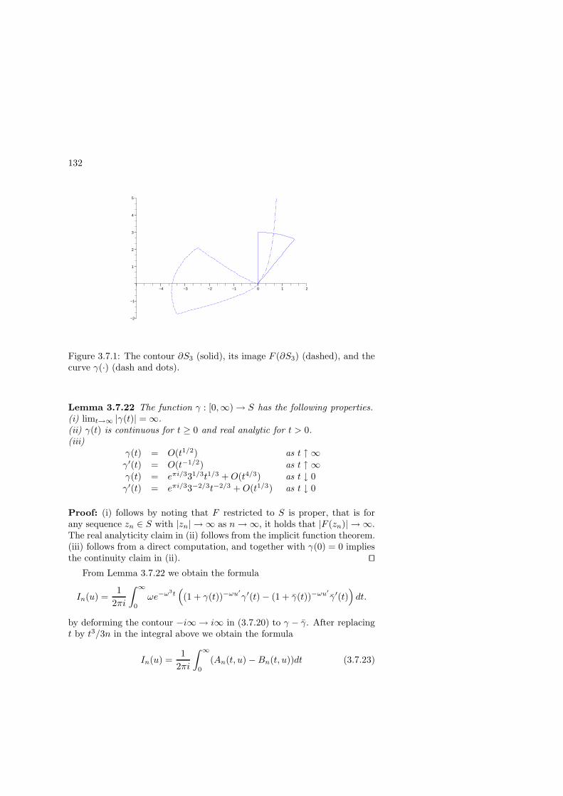
132
−4 −3 −2 −1 0 1 2
−2
−1
1
2
3
4
5
Figure 3.7.1: The contour ∂S3 (solid), its image F (∂S3) (dashed), and thecurve γ(·) (dash and dots).
Lemma 3.7.22 The function γ : [0,∞) → S has the following properties.(i) limt→∞ |γ(t)| = ∞.(ii) γ(t) is continuous for t ≥ 0 and real analytic for t > 0.(iii)
γ(t) = O(t1/2) as t ↑ ∞γ′(t) = O(t−1/2) as t ↑ ∞γ(t) = eπi/331/3t1/3 +O(t4/3) as t ↓ 0
γ′(t) = eπi/33−2/3t−2/3 +O(t1/3) as t ↓ 0
Proof: (i) follows by noting that F restricted to S is proper, that is forany sequence zn ∈ S with |zn| → ∞ as n→ ∞, it holds that |F (zn)| → ∞.The real analyticity claim in (ii) follows from the implicit function theorem.(iii) follows from a direct computation, and together with γ(0) = 0 impliesthe continuity claim in (ii). ut
From Lemma 3.7.22 we obtain the formula
In(u) =1
2πi
∫ ∞
0
ωe−ω3t((1 + γ(t))−ωu′
γ′(t) − (1 + γ(t))−ωu′γ′(t)
)dt.
by deforming the contour −i∞ → i∞ in (3.7.20) to γ − γ. After replacingt by t3/3n in the integral above we obtain the formula
In(u) =1
2πi
∫ ∞
0
(An(t, u) −Bn(t, u))dt (3.7.23)
133
where
An(t, u) = ω exp
(−ω
3t3
3n
)(1 + γ
(t3
3n
))−ωu′
γ′(t3
3n
)t2
n,
Bn(t, u) = ω exp
(−ω
3t3
3n
)(1 + γ
(t3
3n
))−ωu′
γ′(t3
3n
)t2
n.
Put
A(t, u) = exp
(− t
3
3− eπi/3tu+ πi/3
),
B(t, u) = exp
(− t
3
3− e−πi/3tu− πi/3
).
According to (3.7.1) we have
Ai(u) =1
2πi
∫ ∞
0
(A(t, u) −B(t, u))dt. (3.7.24)
A calculus excercise reveals that for any positive constant c,
limn→∞
sup0≤t≤t0
sup|u|<c
∣∣∣∣An(t, u)
A(t, u)− 1
∣∣∣∣ = 0 (3.7.25)
for each t0 ≥ 0 and clearly the analogous limit formula linking Bn(t, u) toB(t, u) holds also. There exist positive constants c1 and c2 such that
| log(1 + γ(t))| ≤ c1t1/3, |γ′(t)| ≤ c2 max(t−2/3, t−1/2)
for all t > 0. There exists a positive constant n0 such that
<(ω3) ≥ n/2, |ω| ≤ 2n1/3, |u′| < 2c
for all n ≥ n0 and |u| < c. Also there exists a positive constant c3 suchthat
ec3t1/3 ≥ t1/6
for t ≥ 1. Consequently there exist positive constants c4 and c5 such that
|ωeω3t(1 + γ(t))−ωu′γ′(t)| ≤ c4n
1/3e−nt/2+c5n1/3tt−2/3
and hence|An(t, u)| ≤ c4e
−t3/6+c5t (3.7.26)
for all n ≥ n0, t > 0 and |u| < c. Clearly we have the same majorizationfor |Bn(t, u)|. Integral formula (3.7.24), uniformity of convergence (3.7.25)

134
and majorization (3.7.26) together are enough to finish the proof of limitformula (3.7.21) and hence of limit formula (3.7.9). ut
Our second application of the steepest descent method is in the follow-ing.
Proof of Lemma 3.7.11 We explain in some detail how to prove (3.7.12)and then we briefly indicate the modifications of the method needed toprove the remaining three formulas.
Recall (3.1.6) in Definition 3.1.5, and by by replacing ζ by x1/2ζ there,deduce the integral representation
Ai(x) =x1/2
2πi
∫
C
ex3/2H(ζ)dζ for x > 0 (3.7.27)
whereH(ζ) = ζ3/3 − ζ.
Consider the image
H(C) = {−t3/3 − eπi/3t|t ≥ 0} ∪ {−t3/3 − e−πi/3t|t ≥ 0}
of the contour C under the map H . The contour H(C) is supported in theleft half-plane, passes through the origin, and is oriented so that the branchbelow (resp., above) the real axis is traversed left to right (resp., right toleft). As in the proof of Lemma 3.7.8, we want to modify the contour C toanother contour, say C′, so that =(H(C′)) is constant, and the deformedcontour C′ “snags” a critical point ζ0 of H , so that the image contourH(C′) satisfies sup<(H(C′)) ≤ <H(ζ0). Now we have H ′(ζ) = ζ2 − 1,hence ζ = ±1 are the critical points of H and H(±1) = ∓2/3 are thecorresponding critical values. The best contour C′ for our purposes “snags”the critical point ζ = 1 and has image H(C′) running on the real axis from−∞ to −2/3 and back.
Again, as in the proof of Lemma 3.7.8, we define the contour C′ im-plicitely. Consider the closed set
S′ = {1 + reiθ |r ≥ 0, θ ∈ [π/3, π/2]}.
For each ρ > 0 let S′ρ be piece-of-pie-shaped closed set obtained by in-
tersecting S′ with the closed disk of radius ρ about 1 and let ∂S′ρ be the
boundary of S′ρ. For all t > 0 and for all sufficiently large ρ, the image curve
H(∂S′ρ) winds exactly once around the point −2/3 − t, see Figure 3.7.2.
Consequently, by the argument principle, the equation H(ζ) = −2/3 − thas for each t > 0 a unique solution γ(t) ∈ S′. Also it is clear that γ(0) = 1is the only solution of the equation H(ζ) = −2/3 in S′. We then havethe following analog of Lemma 3.7.22, whose proof is similar and thereforeomited.

135
−3 −2 −1 0 1 2
−2
−1
1
2
3
4
Figure 3.7.2: The contour ∂S′1.5 (solid), its image H(∂S′
1.5) (dashed), andthe curve γ(·) (dash and dots).
Lemma 3.7.28 The function γ : [0,∞) → S′ has the following properties.(i) limt→∞ |γ(t)| = ∞.(ii) γ(t) is continuous for t ≥ 0 and real analytic for t > 0.(iii)
γ′(t) = 1/(1 − γ(t)2) for t > 0
γ(t) = eπi/331/3t1/3 +O(t−2/3) as t ↑ ∞γ′(t) = eπi/33−2/3t−2/3 +O(t−5/3) as t ↑ ∞γ(t) = 1 + it1/2 +O(t3/2) as t ↓ 0γ′(t) = it−1/2/2 +O(t1/2) as t ↓ 0
Let C′ be the contour consisting of γ with positive orientation plus γ withthe opposite orientation. If we replace C by C′ we leave the integral (3.7.27)unchanged. It follows that
Ai(x) =e−2x3/2/3x1/2
2πi
∫ ∞
0
e−x3/2t(γ′(t) − γ′(t))dt for x > 0, (3.7.29)
whence (3.7.12) by an application of the Laplace transform asymptotics,Lemma D.12. Differentiation of (3.7.29) on both sides with respect to xleads in very similar fashion to (3.7.13). We remark that by developing γ′(t)
136
in a series of half-integral powers of t for small t one can refine (3.7.12) and(3.7.13) to asymptotic expansions.
The starting point for the proof of (3.7.14) and (3.7.15) is the integralformula
Ai(x) =|x|1/2
2πi
∫
C
e|x|3/2G(ζ)dζ for x < 0 (3.7.30)
where
G(ζ) = ζ3/3 + ζ.
To find the best contour C′ with which to replace C consider the wedge-shaped closed sets
S1 ={i+ reiθ
∣∣ t ∈ [0,∞), θ ∈ [π/4, π/3]},
S2 ={i+ reiθ
∣∣ t ∈ [0,∞), θ ∈ [π, π + π/4]}
in the complex plane. One then have the following lemma, whose proof isleft to Exercise 3.7.33.
Lemma 3.7.31 (i) the equation G(ζ) = 2i/3 − t has for each t ≥ 0 aunique solution γj(t) ∈ Sj for j = 1, 2.(ii) the functions γj : [0,∞) → Sj are well-behaved and in particular haveeasily worked out asymptotic behavior as t ↓ 0 and t ↑ ∞. work this out
and write here the results! ??(iii) under replacement of the contour C by the contour C′ = γ1−γ2+γ2−γ1
the integral (3.7.30) does not change.
The proof of (3.7.14) and (3.7.15) follows from Lemma 3.7.31 by the samerecipe that led to to the proof of (3.7.12). ut
Remark 3.7.32 In contrast to the proof of (3.7.12) and (3.7.13) whichinvolves only one critical point of F (ζ), the proof of (3.7.14) and (3.7.15)involves both critical points of G(ζ). In more general applications of steepestdescent it is possible for several critical points to come into play; also onecan have critical points of higher multiplicity.
Proof of Lemma 3.7.4 By (3.7.12), (3.7.13), (3.7.14), (3.7.15), and theAiry differential equation there exists a positive constant C such that
max(|Ai(x)|, |Ai′(x)|, |Ai′′(x)|) ≤ Ce−x
for all real x and hence
|x− y| ≥ 1 ⇒ |A(x, y)| ≤ 2C2e−x−y
137
for all real x and y. But by the variant (3.5.7) of Taylor’s theorem notedabove we also have
|x− y| < 1 ⇒ |A(x, y)| ≤ 2C2e2e−x−y.
Thus the lemma is proved. utExercise 3.7.33 Complete the proof of Lemma 3.7.31.
3.8 Analysis of the Tracy-Widom distribu-
tion and proof of Theorem 3.1.10
We will study the Fredholm determinant
∆ = ∆(t) := 1 +
∞∑
k=1
(−1)k
k!
∫∞t · · ·
∫∞t A
(x1 . . . xk
x1 . . . xk
)∏kj=1 dxj
where A(x, y) is the Airy kernel and as before we write
A
(x1 . . . xk
y1 . . . yk
)=
k
deti,j=1
A(xi, yj).
We are going to explain why ∆(t) is a distribution function, which, to-gether with Theorem 3.1.7, will complete our proof of weak convergence
of n2/3(
λ(n)n√n
− 2). Further, we are going to link ∆(t) to the Painleve II
differential equation.
We begin by putting the study of the Tracy-Widom distribution ∆(t)into a framework compatible with the general theory of Fredholm determi-nants developed in Section 3.4. Let λ denote the unique measure on thereal line such that ∫
f(x)dλ(x) =
∫ ∞
t
f(x)dx
for all integrable f on the line (although λ depends on t, we supress thisdependence from the notation). We have then
∆ = 1 +∞∑
k=1
(−1)k
k!
∫· · ·∫A
(x1 . . . xk
x1 . . . xk
) k∏
j=1
dλ(xj).
Put
H(x, y) = A(x, y) +
∞∑
k=1
(−1)k
k!
∫· · ·∫A
(x x1 . . . xk
y x1 . . . xk
) k∏
j=1
dλ(xj).
138
In view of the basic estimate (3.4.10) and the crude bound (3.7.5) for theAiry kernel, we must have ∆ → 1 as t ↑ ∞. Similarly we have
supt≥t0
supx,y∈R
ex+y|H(x, y)| <∞
for each real t0 and
limt↑∞
supx,y∈R
ex+y|H(x, y) −A(x, y)| = 0.
Note that because ∆ can be extended to a not-identically-vanishing entireanalytic function of t, it follows that ∆ vanishes only for isolated real valuesof t. Put
R(x, y) = H(x, y)/∆,
provided of course that ∆ 6= 0; a similar proviso applies to each of thefollowing definitions since each involves R(x, y). Put
Q(x) = Ai(x) +
∫R(x, y)Ai(y)dλ(y),
P (x) = Ai′(x) +
∫R(x, y)Ai′(y)dλ(y),
q = Q(t), p = P (t),
u =
∫Q(x)Ai(x)dλ(x), v =
∫Q(x)Ai′(x)dλ(x) =
∫P (x)Ai(x)dλ(x),
last equality by symmetry R(x, y) = R(y, x). Convergence of all theseintegrals is easy to check. Note that each of the quantities q, p, u and vtends to 0 as t ↑ ∞. More precisely, q is asymptotic to Ai(t) as t ↑ ∞.
3.8.1 The first standard moves of the game
We follow the trail blazed in the discussion of the sine-kernel in Section 3.6.The first few steps we can get through quickly by analogy. We have
∂
∂tλ = −δt, λ′ = δt, (3.8.1)
∂
∂tlog ∆ = R(t, t), (3.8.2)
∂
∂tR(x, y) = −R(x, t)R(t, y). (3.8.3)

139
As before we have a relation
R(x, y) =Q(x)P (y) −Q(y)P (x)
x− y= R(y, x) (3.8.4)
and hence by L’Hopital’s Rule we have
R(x, x) = Q′(x)P (x) −Q(x)P ′(x). (3.8.5)
We have differentiation formulas
∂
∂tQ(x) = −R(x, t)Q(t) = −Q(t)R(t, x), (3.8.6)
∂
∂tP (x) = −R(x, t)P (t) = −P (t)R(t, x). (3.8.7)
Here the Airy function and its derivative are playing the roles previouslyplayed by sine and cosine, but otherwise to this point our calculation isrunning just as before. Actually the calculation to this point is simplersince we are focusing on a single interval of integration rather than onseveral.
3.8.2 The wrinkle in the carpet
As before we introduce the abbreviated notation
A′(x, y) =
(∂
∂x+
∂
∂y
)A(x, y), R′(x, y) =
(∂
∂x+
∂
∂y
)R(x, y),
(F ?′ G)(x, y) =
∫F (x, z)G(z, y)dλ′(z) = F (x, t)G(t, y).
Here’s the wrinkle in the carpet that changes the game in a critical way:A′ does not vanish identically. Instead we have
A′(x, y) = −Ai(x)Ai(y), (3.8.8)
which is an immediate consequence of the Airy differential equation y′′ −xy = 0. Calculating as before but this time not putting A′ to zero we findthat
R′ = R ?′ R+A′ +R ? A′ +A′ ? R+R ? A′ ? R.
Written out “in longhand” the last equation says that
(∂
∂x+
∂
∂y
)R(x, y) = R(x, t)R(t, y) −Q(x)Q(y). (3.8.9)
140
The wrinkle “propagates” to produce the extra term on the right. We nowhave
Q′(x) = Ai(x) +∫ (
∂∂xR(x, y)
)Ai(y)dλ(y)
= Ai′(x) −∫ (
∂∂yR(x, y)
)Ai(y)dλ(y)
+R(x, t)∫R(t, y)Ai(y)dλ(y) −Q(x)u
= Ai(x) +∫R(x, y)Ai′(y)dλ(y) +
∫R(x, y)Ai(y)dλ′(y)
+R(x, t)∫R(t, y)Ai(y)dλ(y) −Q(x)u
= Ai(x) +∫R(x, y)Ai′(y)dλ(y)
+R(x, t)(Ai(t) +∫R(t, y)Ai(y)dλ(y)) −Q(x)u
= P (x) +R(x, t)Q(t) −Q(x)u.(3.8.10)
Similarly,
P ′(x) = xAi(x) +∫ (
∂∂xR(x, y)
)Ai′(y)dλ(y)
= xAi(x) −∫ (
∂∂yR(x, y)
)Ai′(y)dλ(y)
+R(x, t)∫R(t, y)Ai′(y)dλ(y) −Q(x)v
= xAi(x) +∫R(x, y)yAi(y)dλ(y) +
∫R(x, y)Ai′(y)dλ′(y)
+R(x, t)∫R(t, y)Ai′(y)dλ(y) −Q(x)v
= x(Ai(x) +∫R(x, y)Ai(y)dλ(y))
+∫R(x, y)(y − x)Ai(y)dλ(y)
+R(x, t)(Ai′(t) +∫R(t, y)Ai′(y)dλ(y)) −Q(x)v
= xQ(x) +∫
(P (x)Q(y) −Q(x)P (y))Ai(y)dλ(y)+R(x, t)P (t) −Q(x)v
= xQ(x) +R(x, t)P (t) + P (x)u − 2Q(x)v.(3.8.11)
This is more or less in analogy with the sine-kernel case. But the wrinklecontinues to propagate, producing the extra terms involving the quantitiesu and v.

141
3.8.3 Linkage to Painleve II
The derivatives of the quantities p, q, u and v with respect to t we denotesimply by a prime. We calculate these derivatives as follows. Observe that
q′ =∂
∂tQ(x)
∣∣∣∣x=t
+Q′(t), p′ =∂
∂tP (x)
∣∣∣∣x=t
+ P ′(t).
By adding (3.8.6) to (3.8.10) and (3.8.7) to (3.8.11) we have
q′ = p− qu, p′ = tq + pu− 2qv. (3.8.12)
It follows also via (3.8.5) that
∂
∂tlog ∆(t) = R(t, t) = q′p− p′q = p2 − tq2 − 2pqu+ 2q2v. (3.8.13)
We have
u′ =∫ (
∂∂tQ(x)
)Ai(x)dλ(x) +
∫Q(x)Ai(x)d
(∂λ∂t
)(x)
= −Q(t)∫R(t, x)Ai(x)dλ(x) −Q(t)Ai(t)
= −q2
v′ =∫ (
∂∂tQ(x)
)Ai′(x)dλ(x) +
∫Q(x)Ai′(x)d
(∂λ∂t
)(x)
= −Q(t)∫R(t, x)Ai′(x)dλ(x) −Q(t)Ai′(t)
= −pq.We have a first integral
u2 − 2v = q2;
at least it is clear that the t-derivative here vanishes, but then then constantof integration has to be 0 because all the functions here tend to 0 as t ↑ ∞.Finally
q′′ = (p− qu)′ = p′ − q′u− qu′ = tq + pu− 2qv − (p− qu)u− q(−q2)= tq + pu− 2qv − pu+ qu2 + q3 = tq + 2q3 , (3.8.14)
which is Painleve II.
It remains to prove that F2 is a distribution function. By adding equa-tions (3.8.9) and (3.8.3) we get
(∂
∂x+
∂
∂y+∂
∂t
)R(x, y) = −Q(x)Q(y). (3.8.15)
By evaluating both sides at x = t = y and also using (3.8.2) we get
∂2
∂t2log ∆ = −q2. (3.8.16)

142
Let us now write q(t) and ∆(t) to emphasize the t-dependence. In view ofthe rapid decay of ∆(t) − 1, (log ∆(t))′ and q(t) as t ↑ ∞ we must have
∆ = exp
(−∫ ∞
t
(x− t)q(x)2dx
),
whence (finally!) the conclusion that F2(t) = ∆(t) is a distribution func-tion. Together with (3.8.14) and Theorem 3.1.7, this completes the proofof Theorem 3.1.10. ut
3.9 Bibliographical notes
a lot to do here; what follows is just a random collection moved
from the main body of the text.
The book [Wil78] contains an excellent short introduction to orthogonalpolynomials as presented in Section 3.2.
Our treatment of Fredholm determinants in Section 3.4 is for the mostpart adapted from [Tri85]. The latter gives an excellent short introduc-tion to Fredholm determinants and integral equations from the classicalviewpoint.
Section 3.3.1 follows the very nicely written paper [HT98]. Formula(3.3.13) is due to Haagerup and Thorbjornsen, as is the observation thatdifferential equation (3.3.14) implies a recursion for the moments of LN
discovered by [HZ86] in the course of the latter’s investigation of the modulispace of curves.
The beautiful set of nonlinear partial differential equations (3.6.3), con-tained in Theorem 3.6.2, is one of the great discoveries reported in [JMMS80].We’ll call these the Kyoto equations. To derive the equations we followedthe simplified approach of [TW93]. The differential equations have a Hamil-tonian structure discussed briefly in [TW93]. The same system of partialdifferential equations is discussed in [Mos80] in a wider geometrical context.See also [HTW93].
Limit formula (3.7.9) appears in the literature as [Sze75, Eq. 8.22.14, p.201] but is stated there without much in the way of proof. The importantpaper [PR29] comes very close to supplying a proof of (3.7.9) but strictlyspeaking misses the mark since it is devoted to the asymptotic behavior ofthe Hermite polynomials Hn(x) for real positive x only. But still, the ideasof the latter paper are very robust, and it is on these ideas that we base therelatively short self-contained proof of (3.7.9) presented in Section 3.7.3.[I still must have a look at the Bateman Manuscript Project; perhaps the