introduction to microwaves lectures

Lecture 1

Lecture 1 Objectives• EEE 591/445 is a prerequisite for 545 and 547.• Motivate the study of microwave circuit design.

– Study from the aspects of microwave circuit design.– Review skills that students should have developed in previous

classes (or from work experience).– Prepare students toward real-world project with tools

• Field based HFSS• Circuit based ADS• Combined HFSS and ADS simulations

• These classes build-up ground for Microwave systems– Wire-less communications– Defense industry: high resolution radars, SLAR, SAR, Microwave

radiometers– RF Heating, microwave oven, welding, etc.– Health care industry, MRI, CT, physical therapy

1

Lecture 1 2

Microwave generated images by side looking airborne radar (SLAR)

Courtesy: Microwave Remote Sensing by Ulaby, Moore and Fung

Lecture 1 3

Passive remote sensing: images by microwave radiometer


Lecture 1 4

Prototype Whole Body TEM Coil @ 4T M

RI

RF

coil

an

d t

he i

mag

es:

Cou

rtesy

MR

In

stru

men

ts,

Inc.

Lecture 1

What is a “Microwave”• “Micro”= small• Electromagnetic waves with small wavelength• Small: 1 meter to 1 mm• Frequency range: 300 MHz to 300 GHz• “Classical” microwave frequency range: 1 GHz

to 30 GHz

5

Lecture 1

What are some systems whose RF portion works in the frequency range of 300 MHz to 300 GHz?

• UHF SATCOM (military)• UHF TV• Cell phones• Wireless LANs• Radar (aviation,

military, weather, GPR)• Public service radios

(police, fire)• Radio astronomy• Communication with

space probes

• Business and family service radios

• Amateur radio• GPS• Microwave ovens• Secure comm systems

for the military (LPI/LPD)

• DBS• MMDS

6

Lecture 1

Microwave Engineering• Microwave frequency range: 300 MHz to 300

GHz.• Below 300 MHz, we can usually use circuit theory

to design RF portion of transceiver. – ADS (Advanced Device Simulator)– At worst, only the antenna needs to be analyzed using

full electromagnetic theory (Maxwell’s equations), HFSS (high frequency structure simulator)

• Above 300 GHz, we can usually use geometric optics (ray tracing) to design systems.

7

Lecture 1

Microwave Engineering (Cont’d)• Both circuit theory and geometric optics are

special cases of the more general theory of electromagnetism (Maxwell’s equations).

• In the microwave frequency range, neither of these approximations can be used to completely characterize the system. – Circuit theory can often be used to analyze much

of the system from 300 MHz to 10 GHz.– Geometric optics can often be used to analyze

much of the system above 60 GHz.

8

Lecture 1

Why do satellite based systems tend to use microwave frequency range?

• More bandwidth and hence information carrying capacity is available.

• Atmosphere is “transparent” to electromagnetic radiation from about 30 MHz to about 30 GHz (radio window).

9


Lecture 1

Classifications of Microwave Systems• Noise limited vs interference limited• Government (military, non-military) vs commercial• QoS (quality of service) driven vs capacity driven• Example of a Microwave System: Cell Phone:Interference limited, commercial, capacity driven

– Complete system must cost $1s or $10s per unit– Business is highly commoditized– Technology choices will tend to focus on RF-CMOS single chip

solutions to drive down cost; performance is a secondary issue.

•

10

Lecture 1

Example: Microwave System: Radio Telescope

• Noise limited, government (non-military), QoS driven– Complete system may cost $100k’s per unit– Only one or a few units are ever constructed– Technology choices tend to focus on high quality

discrete components; performance is tantamount; cost is a secondary factor.

11

Lecture 1

Aspects of Microwave Circuit Design• Antenna design• Transmission media design (microstrip, stripline,

waveguide, etc.)• Matching network design (L-networks, single- and double-

stub matching, multi-section transformers, etc.) • Signal (power) distribution (power dividers, and hybrid

couplers, etc.)• Analog signal processing (e.g., amplitude and phase

tapering; attenuators, phase-shifters, etc.)• Filter design• Low noise or power amplifier design and use in a system

(noise and linearity issues).• Mixer design• Oscillator design• SELECTED THREE DESIGNS: MRI, Transceiver, LEPA

12

Lecture 1

MRI 23cm TEM Coil for 2dB more gain

Short Coil Option Multiple transmission line

13

Lecture 1

0

s

lT

ls

ls

h

h

A-A

Tuning stub

Shielding

Magnetic field distribution

around field of view

Schematic view and Cross-section view

14

Lecture 1

Multiple transmission line: Parameters found by MoM

Coaxial line passive loads

Coaxial line passive loads

15

Lecture 1

Case Study: C/Ku Band Earthstation Antennas

ATCi Corporate Headquarters450 North McKemyChandler, AZ 85226 USA

SimulsatParabolicHorn feed Multiple horn feeds

16

Lecture 1


Incoming plane wave is focused by reflector at location of horn feed.

Feed horn is designed so that it will illuminate the reflector in such a way as to maximize the aperture efficiency.

17

Lecture 1

A planar orthomode transducer (OMT) is used to achieve good isolation between orthogonal linear polarizations.


18

Feed horn needs to be able to receive orthogonal linear polarizations (V-pol and H-pol) and maintain adequate isolation between the two channels.

Lecture 1


Horn

Feed waveguide (WR 229)

To LNB

Stripline circuit with OMT, ratrace and WR229 transitions

19

Lecture 1


Single-ended probe

Differential-pair probes

Ratrace hybrid

WR229Transitions

50 ohm transmission line

Layout of the stripline trace layer

Vias

20

Lecture 1

Case Study: C/Ku Band Earthstation Antennas Analysis of ratrace hybrid in ADS

21

Lecture 1

Case Study: C/Ku Band Earthstation Antennas Resulting layout of ratrace hybrid for analysis in Momentum

Port 1

Port 4

Port 3 Port 2

22

Lecture 1


The two linear polarizations each are fed to a LNB (low noise block).

LNB

LNB

23

LNB:

LNA Mixer

IF Output:950-2150 MHz(To Receiver)

Local Oscillator

BPF

Lecture 1


Analysis of Design in ADS

S2PSNP5

21

Ref

S2PSNP6

2 1

Ref

TermTerm1

Z=50 OhmNum=1

S4PSNP4

4

1 2

3 Ref

S3PSNP3

2

3Ref

1

TermTerm2

Z=50 OhmNum=2

RR1R=50 Ohm

S_ParamSP1

Step=0.1 GHzStop=4.8 GHzStart=3.2 GHz

S-PARAMETERS

WR229 Transitions

Horn

Ratrace Hybrid

24

Lecture 1

Combined HFSS-ADI simulation

• Lens enhanced phase array for 60 GHz antennas– Hybrid LEPA configuration

1

2

1 2

10

60

20

10

2.5

L mm

L mm

F mm

G mm

a a mm

25

Lecture 1

Lens enhanced phased array for 60 GHz antennas

• Beam-Steerable Antennas are important for radio communication at high frequencies the directivity of the antenna constitutes an

essential term in the link budget steer-ability is necessary for sustaining

connectivity between mobile nodes.

• Common Methods of Implementation Phased Array Transceivers with bipolar or CMOS

integrated phase shifters Planar Lens-Array Antennas combined with a

switchable array of feed antennas at their focal plane

26

Lecture 1

IntroductionAdvantages Limitations

Phased Array Approach

Phased array transceivers with bipolar or CMOS integrated phase shifters have been extensively researched in recent years, in both industry and academia.

The maximum practical size of the array is restricted to smaller than 8 × 8, or more realistically 4 × 4.

Planar Lens-array Approach

The elimination of the phase shifters and lossy feed networks renders this approach low cost and easily scalable.

(1) discrete beam positions(2) need for RF switches(3) relatively large depth(4) widely spread feed array

geometry(5) Not available for compact

devices

27

Lecture 1

• Lens-Enhanced Phased Array (LEPA) consists of a small phased array and significantly larger lens-array.

• Replacing the feed array with the phased array, it offers several advantages: reduces the depth of the system (from F to G) eliminates the need for RF switches enables high resolution scanning allows for some level of power combining rather than putting

the burden of radiation on a single feed at any given time• We examine the feasibility of this approach via a 60 GHz case

study.

28

Lens enhanced phased array for 60 GHz antennas

Lecture 1

Base Line Designs• We first simulate two cases: The PA radiating alone and the LA being

excited by actual switchable point-source feeds.

Figure 2 Simulated radiation pattern of the 4×4 PA for (0,0) and (45,45) scan angles.

Figure 3 Simulated radiation pattern of the 24×24 LA for (0,0) and (45,45) scan angles (F=20 mm).

The dramatic drop in directivity indicates a poor scan performance that is characteristic of shallow lenses (F/D <1, where D is the lens diameter).

29

Lecture 1

LEPA Simulations with Virtual Point Source

(a) (b)

(d) (c)

Figure 4 Simulation results for LEPA set for radiation towards (0,0). Calculations for F= 20 mm, G= 10 mm. Green squares on (b), (c) indicate the “lit” region in each case. (a) PA phase profile, (b) LA output phase, (c) LA output amplitude, (d) radiation pattern.

30

Lecture 1

LEPA Simulations with Virtual Point Source

(a) (b)

(d) (c)

Fig

ure

5 S

am

e a

s F

ig.4

wit

h L

EP

A s

et

to s

can

to

(4

5,4

5).

31

Lecture 1

LEPA with Improved Lens DesignF

ig.

9 t

he fi

nal

sim

ula

ted

ou

tpu

t p

hase

acr

oss

th

e l

en

s an

d r

ad

iati

on

p

att

ern

s fo

r th

e (

a)

(0,0

) an

d (

b)

(45,4

5)

beam

an

gle

s.

32

(a). Normal incidence: Phase and amplitude

(b). Oblique incidence: Phase and amplitude

Lecture 1

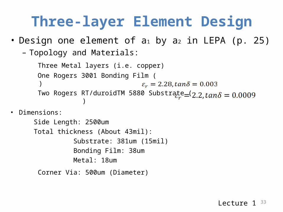
Three-layer Element Design• Design one element of a1 by a2 in LEPA (p. 25)

– Topology and Materials:

Three Metal layers (i.e. copper)

One Rogers 3001 Bonding Film ( )

Two Rogers RT/duroidTM 5880 Substrate ( )

• Dimensions:

Side Length: 2500um

Total thickness (About 43mil):

Substrate: 381um (15mil)

Bonding Film: 38um

Metal: 18um

Corner Via: 500um (Diameter)

33

Lecture 1

Three-layer Element Design (HFSS) 3-pole (red) 4-pole (blue)

45.00 50.00 55.00 60.00 65.00 70.00 75.00Freq [GHz]

-60.00

-50.00

-40.00

-30.00

-20.00

-10.00

0.00

dB

-200.00

-150.00

-100.00

-50.00

0.00

50.00

100.00

150.00

200.00

de

g

45.00 50.00 55.00 60.00 65.00 70.00 75.00Freq [GHz]

-60.00

-50.00

-40.00

-30.00

-20.00

-10.00

0.00

dB

-200.00

-150.00

-100.00

-50.00

0.00

50.00

100.00

150.00

200.00

de

g

34

Lecture 1

Simplified Geometry of 32 GHz LEPA Unit

Bottom Slot Antenna

Top Slot Antenna

Slot Line Resonator

Eout

Einc

x

y

Top View from positive Z-axis

Substrate: Rogers RT/duroid 5880h=381um=15mil

Copper

(zero thickness for simple) Bonding film ~ 38um

35

Lecture 1

Created 3D Geometry Model in HFSS

• element

36

Lecture 1

Setting Boundaries and Excitation• For FSS (frequent selective surface) structures, we use

Master/Slave boundaries and Floquet Port in HFSS. • Master and Slave Boundaries enable you to model planes of

periodicity where the E-field on one surface matches the E-field on another to within a phase difference. – They force the E-field at each point on the slave boundary match that

at corresponding point on the master boundary. They are useful for simulating devices such as infinite arrays.

• Floquet Port in HFSS is used exclusively with planar-periodic structures. Chief examples are planar phased arrays and frequency selective surfaces when these may be idealized as infinitely large. The analysis of the infinite structure is then accomplished by analyzing a unit cell.

• To create “AirBox” Position (-2340, -2340, -4381) XSize 4680; YSize 4680; ZSize 8800 37

Lecture 1

Setting Boundaries and Excitation• After finishing the above settings

for Master1 and Slave1, you can see the boundary condition like the right figure.

• It is similar to set Master2 and Slave2 on the other sets of side faces.

It is easier to set FloquetPort2 on the bottom face, for you will find that A and B direction are done already according to the previous settings in FloquetPort1. 38

Lecture 1

Analyzing and Creating Solution Reports

• Be sure to save the project in time!• To run the project:• HFSS > Analyze all• To create reports:• HFSS > Results > Create Rectangular Report• Report Window:Solution: Setup1 Sweep1Domain: SweepCategory: S ParameterQuantity: S(FloquetPort1:1, FloquetPort1:1) => S11 S(FloquetPort1:1, FloquetPort2:2) => S12Function: we choose dB for amplitude and deg for phase Note: We use two modes to represent polarization rotation in this case.

The choice of Quantity depends on what are Mode 1 and 2. You can check them in Project Manager Window > PortField Display to make sure the right S parameters are displayed.

39

Lecture 1

Analyzing and Creating Solution Reports• Solution report from HFSS

24.00 26.00 28.00 30.00 32.00 34.00 36.00 38.00 40.00Freq [GHz]

-50.00

-40.00

-30.00

-20.00

-10.00

0.00

dB

-200.00

-150.00

-100.00

-50.00

0.00

50.00

100.00

150.00

200.00

de

g

Ansoft LLC HFSSDesign1XY Plot 1 ANSOFT

40

Lecture 1

Co-simulation with HFSS and ADS• To generate .sNp file from HFSS• HFSS > Results > Solution Data > Export Matrix Data• Save the solution as sNp file

• To load S parameters to ADS, in the ADS:• Data Items > S4PFind the *.s4p file by “browse”File type: Touchstone• Add Term and Ground to each port and set Z0=375 ohm (because of de-

embeding in HFSS)

• Then you can do the simulation and plot S parameter results of HFSS in ADS.

• S11: S(FloquetPort1:1, FloquetPort1:1) S(1,1)• S12: S(FloquetPort1:1, FloquetPort2:2) S(1,4)

Phys. HFSS ADS

mode/polarization

41

Lecture 1

Co-simulation with HFSS and ADS

• To plot S parameter results of HFSS in ADS.

26 28 30 32 34 36 3824 40

-40

-30

-20

-10

-50

0

-100

0

100

-200

200

freq, GHz

dB(S

(1,1

))dB

(S(1

,4))

phase(S(1,4))

42

Lecture 1

Equivalent Circuit

• Equivalent circuit of AFA structure.• Here I use Tlines-Stripline for parameters in the table. You

can also use Tlines-Ideal as the figure shows.

Ra 500Ω

Ca 1.03pf

La 0.0218nH

n 0.293

Cf 0.0097pf

W 225um

L 2860um

43

Lecture 1

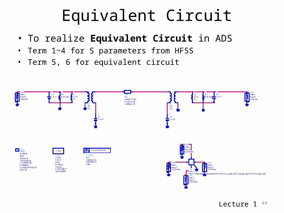
Equivalent Circuit• To realize Equivalent Circuit in ADS• Term 1~4 for S parameters from HFSS• Term 5, 6 for equivalent circuit

S_ParamSP1

Step=Stop=40 GHzStart=24 GHz

S-PARAMETERS

TermTerm3

Z=375 OhmNum=3

TermTerm5

Z=50 OhmNum=5

TermTerm6

Z=50 OhmNum=6

TermTerm2

Z=375 OhmNum=2

TermTerm4

Z=375 OhmNum=4

TermTerm1

Z=375 OhmNum=1

SLINTL5

L=2860 um {t}W=225 um {t}Subst="SSub1"

VARVAR1

f=33.6 {t}L=1.0/(2*pi*f*1e9)̂ 2/CL1=2820e-6C=1.03e-012 {t}Cf=9.7e-015 {t}n=0.293 {t}f0=32R=500 {t}

EqnVar

S4PSNP3File="C:\Users\lzhang95\Desktop\SNP \AAFA_32_3_pole_375_T_sample_steps1 HFSSDesign1.s4p"

4

1 2

3 R e f

CC2C=Cf F

CC1C=Cf F

TFTF1T=n

TFTF2T=n

RR1R=R Ohm

RR3R=R Ohm

CC3C=C F

LL1

R=L=L H

LL2

R=L=L H

CC4C=C F

SSUBSSub1

TanD=0.0009Cond=5.88E+7T=18 umB=750 umMur=1Er=2.2

SSub

44

Lecture 1

Co-simulation with HFSS and ADS• Tune ADS result (blue) according to that from HFSS (red).

24 26 28 30 32 34 36 3822 40

-50

-40

-30

-20

-10

-60

0

freq, GHz

dB(S

(1,1

))dB

(S(1

,4))

dB(S

(5,5

))dB

(S(5

,6))

24 26 28 30 32 34 36 3822 40

-100

0

100

-200

200

freq, GHz

phas

e(S(

1,4)

)ph

ase(

S(5,

6))

45

introduction to microwaves lectures

Documents