INTRODUCTION TO

MATLAB

Kadin Tseng

Boston University

Scientific Computing and Visualization

It is developed by The Mathworks, Inc. (http://www.mathworks.com)

It is an interactive, integrated, environment

• for numerical/symbolic, scientific computations and other apps.

• shorter program development and debugging time than traditional

programming languages such as FORTRAN and C.

• slow (compared with FORTRAN or C) because it is interpreted.

• automatic memory management; no need to declare arrays.

• intuitive, easy to use.

• compact notations.

Introduction to MATLAB 2

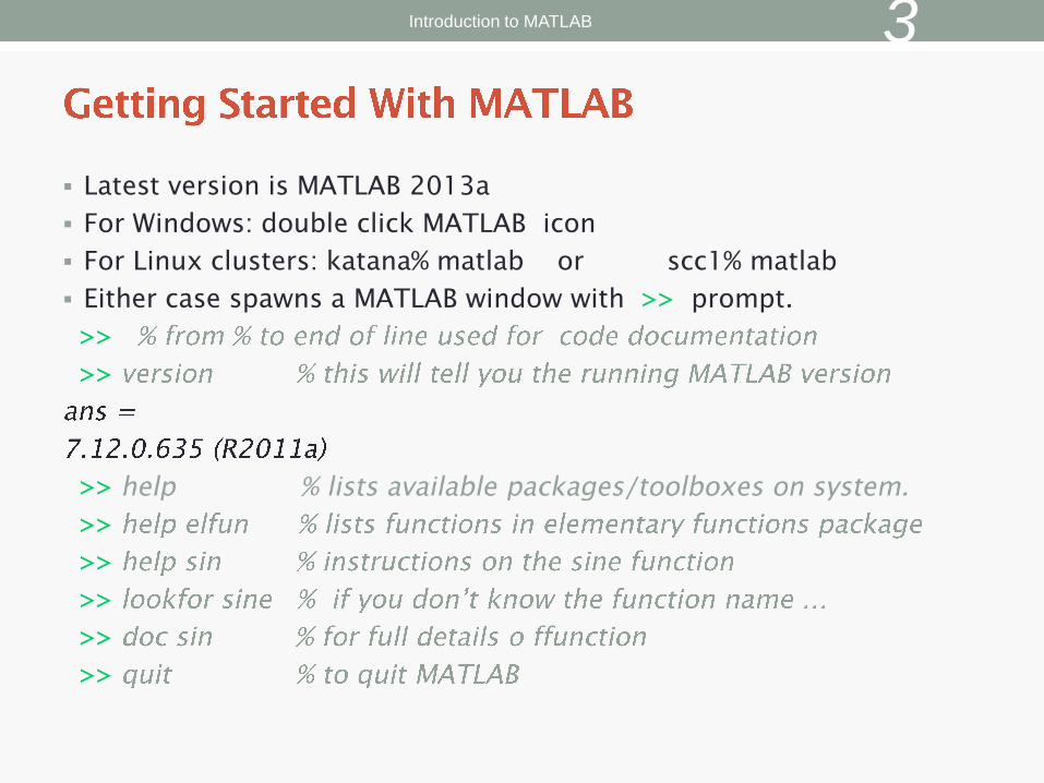
Latest version is MATLAB 2013a

For Windows: double click MATLAB icon

For Linux clusters: katana% matlab or scc1% matlab

Either case spawns a MATLAB window with >> prompt.

>>

>>

>>

>>

>>

>>

>>

>>

Introduction to MATLAB 3

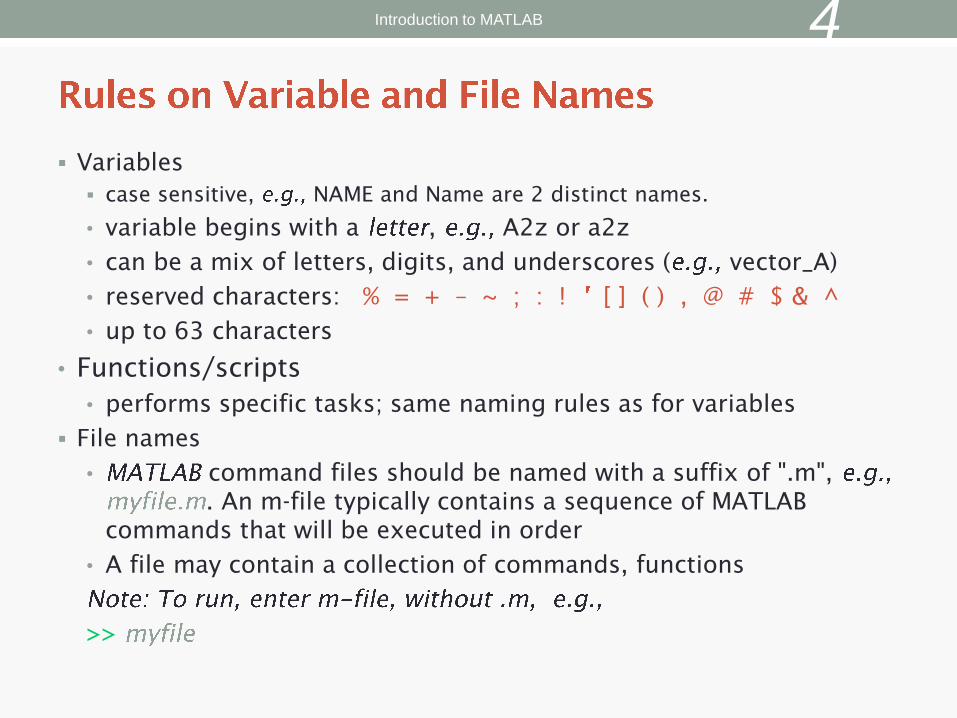
Variables

case sensitive, NAME and Name are 2 distinct names.

• variable begins with a , A2z or a2z

• can be a mix of letters, digits, and underscores ( vector_A)

• reserved characters: % = + – ~ ; : ! [ ] ( ) , @ # $ & ^

• up to 63 characters

• Functions/scripts

• performs specific tasks; same naming rules as for variables

File names

• command files should be named with a suffix of ".m",

. An m-file typically contains a sequence of MATLAB

commands that will be executed in order

• A file may contain a collection of commands, functions

>>

Introduction to MATLAB 4

• Some characters are by for various purposes. Some

as arithmetic or matrix operators: =, +, , *, / , \ and others are used

to perform a multitude of operations. Reserved characters cannot be

used in variable or function names.

• >>

>>

• >>

a =

3

• >>

>>

• >>

>>

• >>

d =

6

,

Introduction to MATLAB 5

• >>

x =

1 3 5 7 9

• >>

y =

3 4 5

• >>

X =

1 2 3

4 5 6

• >>

ans =

6

Introduction to MATLAB 6

>>

>>

>>

x =

1

2

3

>>

ans =

2 3

>>

ans =

6

Introduction to MATLAB 7

• >>

Volume in drive C has no label.

Volume Serial Number is 6860-EA46

Directory of C:\Program Files\MATLAB704\work

01/31/2007 10:56 AM <DIR> .

01/31/2007 10:56 AM <DIR> ..

06/13/2006 12:09 PM 12 foo.exe

06/13/2006 08:57 AM 77 mkcopy.m

• >>

total 0

-rw-r--r-- 1 kadin scv 0 Jan 19 15:53 file1.m

-rw-r--r-- 1 kadin scv 0 Jan 19 15:53 file2.m

-rw-r--r-- 1 kadin scv 0 Jan 19 15:53 file3.m

>>

Introduction to MATLAB 8

>>

>>

>>

5 7 9

>>

A =

1 2 3

4 5 6

>>

B =

1 4

2 5

3 6

Other ways to create B ? (hint: with and )

Introduction to MATLAB 9

>>

C =

14 32

32 77

>>

D =

1 4 9

16 25 36

>>

E =

1 1 1

1 1 1

>>

Your variables are:

A B C D E a b d

Introduction to MATLAB 10

>>

Name Size Bytes Class Attributes

A 2x3 48 double

B 3x2 48 double

C 2x2 32 double

D 2x3 48 double

E 2x3 48 double

a 1x3 24 double

b 1x3 24 double

c 1x3 24 double

>>

>>

Name Size Bytes Class

A 2x3 24 single

>>

Introduction to MATLAB 11

Utilities to initialize or define arrays:

Trigonometric and hyperbolic functions :

These utilities can be used on scalar or vector inputs

>>

Introduction to MATLAB 12

Scalar operation . . .

for j=1:3 % columns

for i=1:3 % rows

a(i,j) = rand; % a(i,j) = random number

b(i,j) = 0; % b(i,j) = 0 unless . . .

if a(i,j) > 0.5

b(i,j) = 1;

end

end

end

Equivalent vector operations . . .

A = rand(3); % A is a 3x3 random number double array

B = zeros(3); % Initialize B as a 3x3 array of zeroes

B(A > 0.5) = 1; % set to 1 all elements of B for which A > 0.5

Introduction to MATLAB 13

A cell array is a special array of arrays. Each element of the cell

array may point to a scalar, an array, or another cell array.

>>

>>

>>

>>

C =

[2x2 double] [1x3 double] {1x1 cell}

[2x1 double] ‘This is a string.‘ []

>>

ans =

1 3

4 2

>>

Related utilities:

Introduction to MATLAB 14

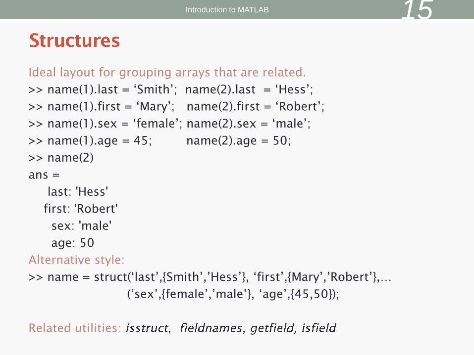
Ideal layout for grouping arrays that are related.

>> name(1).last = ‘Smith’; name(2).last = ‘Hess’;

>> name(1).first = ‘Mary’; name(2).first = ‘Robert’;

>> name(1).sex = ‘female’; name(2).sex = ‘male’;

>> name(1).age = 45; name(2).age = 50;

>> name(2)

ans =

last: 'Hess'

first: 'Robert'

sex: 'male'

age: 50

Alternative style:

>> name = struct(‘last’,{Smith’,’Hess’}, ‘first’,{Mary’,’Robert’},…

(‘sex’,{female’,’male’}, ‘age’,{45,50});

Related utilities:

Introduction to MATLAB 15

There are many types of files in MATLAB.

Only script-, function-, and mat-files are covered here:

1.script m-files (.m) -- group of commands; reside in base workspace

2.function m-files (.m) -- memory access controlled; parameters passed

as input, output arguments; reside in own workspace

3.mat files (.mat) -- binary (or text) files handled with and

4.mex files (.mex) -- runs C/FORTRAN codes from m-file

5.eng files (.eng) -- runs m-file from C/FORTRAN code

6.C codes (.c) – C codes generated by MATLAB compiler

7.P codes (.p) – converted m-files to hide source for security

Introduction to MATLAB 16

If you have a group of commands that are expected to be executed

repeatedly, it is convenient to save them in a file . . .

>> edit mytrig.m % enter commands in editor window

Select File/Save to save it as mytrig.m

A script shares same memory space from which it was invoked.

Define x, then use it in mytrig.m (mytrig can “see” x):

>>

>>

a = 0.5000

b = 0.8660

Script works as if sequentially inserting the commands in mytrig.m at the >>

Introduction to MATLAB 17

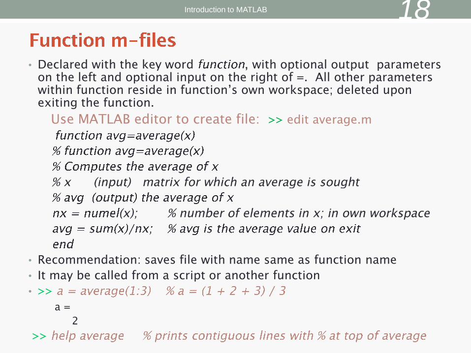
• Declared with the key word , with optional output parameters

on the left and optional input on the right of =. All other parameters

within function reside in function’s own workspace; deleted upon

exiting the function.

Use MATLAB editor to create file: >> edit average.m

• Recommendation: saves file with name same as function name

• It may be called from a script or another function

• >>

a =

2

>>

Introduction to MATLAB 18

Scripts

• Pros:

- convenient; script’s variables are in same workspace as caller’s

• Cons:

- slow; script commands loaded and interpreted each time used

- risks of variable name conflict inside & outside of script

Functions

• Pros:

• Scope of function’s variables is confined to within function. No

worry for name conflict with those outside of function.

• What comes in and goes out are tightly controlled which helps when

debugging becomes necessary.

• Compiled the first time it is used; runs faster subsequent times.

• Easily be deployed in another project.

• Auto cleaning of temporary variables.

• Cons:

• I/O are highly regulated, if the function requires many pre-defined

variables, it is cumbersome to pass in and out of the function – a

script m-file is more convenient.

Introduction to MATLAB 19

>> % creates a special matrix; handy for testing

>> zeros(n,m) % creates matrix of (0)

>> ones(n,m) % creates matrix of (1)

>> rand(n,m) % creates matrix of random numbers

>> repmat(a,n,m replicates by rows and columns

>> diag(M) % extracts the diagonals of a matrix M

>> help elmat % list all elementary matrix operations ( or )

>> abs(x); % absolute value of

>> exp(x); % to the x-th power

>> fix(x); % rounds x to integer towards 0

>> log10(x); % common logarithm of x to the base 10

>> rem(x,y); % remainder of x/y

>> mod(x, y); % modulus after division – unsigned rem

>> sqrt(x); % square root of x

>> sin(x); % sine of x; x in radians

>> acoth(x) % inversion hyperbolic cotangent of x

Introduction to MATLAB 20

>> help % Fastest Fourier Transform in the West

>> help odeexamples % dfferent ODE examples

>> help spline % cubix spline interpolation

>> help eig % eigenvalues & vectors

>> help linsolve % solves Ax=b with LU factorization

>> help visdiff % compare two files or folders (m-file, mat-file,…)

Introduction to MATLAB 21

Create new images

Line plot

Bar graph

Surface plot

Contour plot

Render data or pre-existing images

imread

imshow

imagesc

MATLAB tutorial on 2D, 3D visualization tools as well as other graphics

packages available in our tutorial series.

Introduction to MATLAB 22

Introduction to MATLAB 23

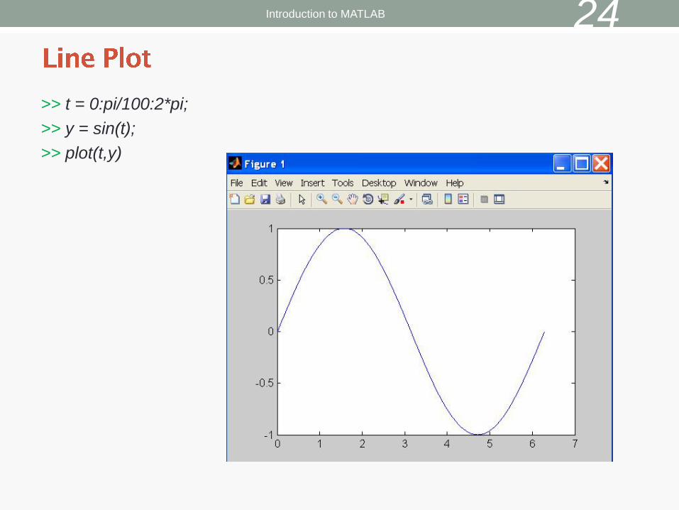
>> t = 0:pi/100:2*pi;

>> y = sin(t);

>> plot(t,y)

Introduction to MATLAB 24

>> xlabel(‘t’);

>> ylabel(‘sin(t)’);

>> title(‘The plot of t vs sin(t)’);

Introduction to MATLAB 25

>> y2 = sin(t-0.25);

>> y3 = sin(t+0.25);

>> plot(t,y,t,y2,t,y3) % make 2D line plot of 3 curves

>> legend('sin(t)','sin(t-0.25)','sin(t+0.25',1)

Introduction to MATLAB 26

Generally, MATLAB’s default graphical settings are adequate which make

plotting fairly effortless. For more customized effects, use the get and set

commands to change the behavior of specific rendering properties.

>> hp1 = plot(1:5) % returns the handle of this line plot

>> get(hp1) % to view line plot’s properties and their values

>> set(hp1, ‘lineWidth’) % show possible values for lineWidth

>> set(hp1, ‘lineWidth’, 2) % change line width of plot to 2

>> gcf % returns current figure handle

>> gca % returns current axes handle

>> get(gcf) % gets current figure’s property settings

>> set(gcf, ‘Name’, ‘My First Plot’) % Figure 1 => Figure 1: My First Plot

>> get(gca) % gets the current axes’ property settings

>> figure(1) % create/switch to Figure 1 or pop Figure 1 to the front

>> clf % clears current figure

>> close % close current figure; “close 3” closes Figure 3

>> close all % close all figures

Introduction to MATLAB 27

>> x = magic(3); % generate data for bar graph

>> bar(x) % create bar chart

>> grid % add grid for clarity

Introduction to MATLAB 28

• Many MATLAB utilities are available in both command and function forms.

• For this example, both forms produce the same effect:

• >> print –djpeg mybar % print as a command

• >> print('-djpeg', 'mybar') % print as a function

• For this example, the command form yields an unintentional outcome:

• >> myfile = 'mybar'; % myfile is defined as a string

• >> print –djpeg myfile % as a command, myfile is treated as text

• >> print('-djpeg', myfile) % as a function, myfile is treated as a variable

% i.e., ‘mybar’ is passed into print

• Other frequently used utilities that are available in both forms are:

• save, load

Introduction to MATLAB 29

>> Z = peaks; % generate data for plot; peaks returns function values

>> surf(Z) % surface plot of Z

Try these commands also:

>> shading flat

>> shading interp

>> shading faceted

>> grid off

>> axis off

>> colorbar

>> colormap(‘winter’)

>> colormap(‘jet’)

Introduction to MATLAB 30

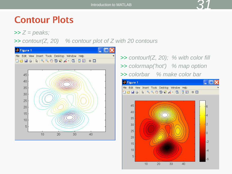
>> Z = peaks;

>> contour(Z, 20) % contour plot of Z with 20 contours

>> contourf(Z, 20); % with color fill

>> colormap('hot') % map option

>> colorbar % make color bar

Introduction to MATLAB 31

Introduction to MATLAB 32

• How to import data (including images in jpg, png, … format)

( read with imread, show with imshow )

• Get on the web, look for an image and save it as, say, myimage.jpg

• >> M = imread(‘myimage.jpg’); % read the image file into a MATLAB array

• >> size(M) % get size of data set; 3rd index represents RGB

• >> imshow(M) % one way to render the image

• >> imagesc(M) % another way

• Export image to file with

• GUI

• Select Export from figure window’s File menu, pick format from save as type, then Save

• MATLAB Command

• imwrite(M, ‘-djpeg’)

• print –djpeg M myfile

(www.bu.edu/tech/research)

www.bu.edu/tech/accounts/special/research/accounts

•

•

• Web-based tutorials

(www.bu.edu/tech/about/research/training/live-tutorials)

(MPI, OpenMP, MATLAB, IDL, Graphics tools)

• HPC consultations by appointment

• Kadin Tseng (kadin@bu.edu)

• Yann Tambouret (yannpaul@bu.edu)

Introduction to MATLAB 33