introduction to machine learning · introduction to machine learning fei li m.s. student in...
TRANSCRIPT

Introduction to Machine Learning
Fei Li M.S. Student in Computer Science
Louisiana State University 04/05/2017

Machine Learning Everywhere!
Face Recognition
Sentiment Analysis
National Defense
Cancer Cell Detection
Natural Language Processing
What is Machine Learning?
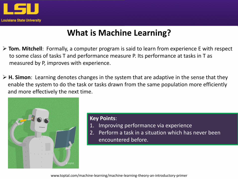
Tom. Mitchell: Formally, a computer program is said to learn from experience E with respect to some class of tasks T and performance measure P. Its performance at tasks in T as measured by P, improves with experience. H. Simon: Learning denotes changes in the system that are adaptive in the sense that they enable the system to do the task or tasks drawn from the same population more efficiently and more effectively the next time.
Key Points: 1. Improving performance via experience 2. Perform a task in a situation which has never been
encountered before.
www.toptal.com/machine-learning/machine-learning-theory-an-introductory-primer
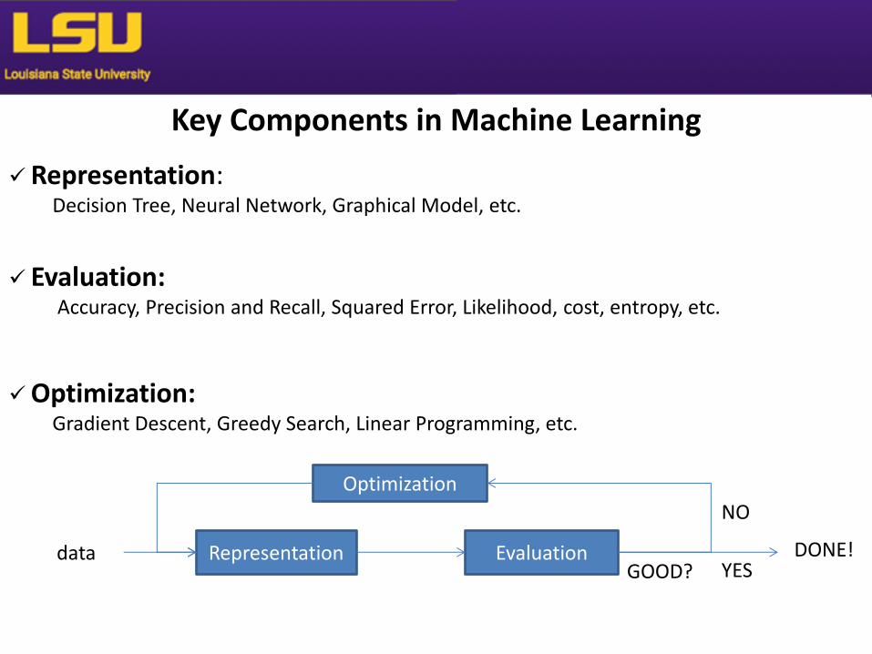
Key Components in Machine Learning
Representation: Decision Tree, Neural Network, Graphical Model, etc.
Evaluation: Accuracy, Precision and Recall, Squared Error, Likelihood, cost, entropy, etc.
Optimization: Gradient Descent, Greedy Search, Linear Programming, etc.
Representation Evaluation
Optimization
data GOOD? YES
NO
DONE!

Application Example: Image Classification
“Motorcycle”
Input: X Output: Y
Source: slides from Prof. Mingxuan Sun, Lousisana State University
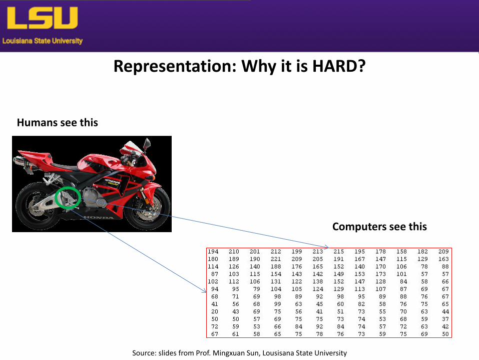
Representation: Why it is HARD?
Humans see this
Computers see this
Source: slides from Prof. Mingxuan Sun, Lousisana State University

handles
wheels
Learning Algorithms
motorcycle
others
Source: slides from Prof. Mingxuan Sun, Lousisana State University

Machine Learning: Evaluation
A dataset Fields class 1.4 2.7 1.9 0 3.8 3.4 3.2 0 6.4 2.8 1.7 1 4.1 0.1 0.2 0 etc …
1.4
2.7
1.9
0.7 (0) Error=0.7
Compare with the target output
https://www.macs.hw.ac.uk/~dwcorne/Teaching/introdl.ppt
Neural Network Model
actual output target
output

Adjust weights based on error
1.4
2.7
1.9
0.7 (0) Error=0.7
Repeat this thousands, maybe millions of times – each time taking a random training instance, and making slight weight adjustments Algorithms for weight adjustment are designed to make changes that will reduce the error
https://www.macs.hw.ac.uk/~dwcorne/Teaching/introdl.ppt
Machine Learning: Optimization
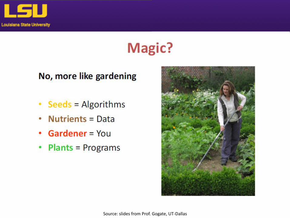
Source: slides from Prof. Gogate, UT-Dallas

Source: slides from Prof. Gogate, UT-Dallas

Summary
Applications
Definitions
Machine Learning = Representation + Evaluation + Optimization
When to Use Machine Learning?

Machine Learning in HPC
Environments
Feng Chen
HPC User Services
LSU HPC & LONI
Louisiana State University
Baton Rouge
April 5, 2017

Topics To Be Discussed
Fundamentals about Machine Learning
What is a neural network and how to train it
Build a basic 1-layer neural network using Keras/TensorFlow
MNIST example
– Softmax classification
– Cross-entropy cost function
– How to add more layers
– Dropout, learning rate decay...
– How to build convolutional networks
How to utilize HPC for hyperparameter test?
04/05/2017 Machine Learning in HPC Environments Spring 2017 2
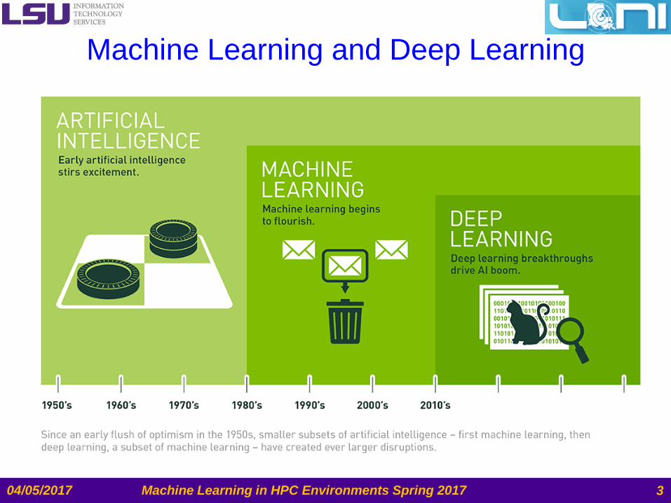
Machine Learning and Deep Learning
04/05/2017 Machine Learning in HPC Environments Spring 2017 3

Machine Learning
Machine Learning is the ability to teach a computer without explicitly
programming it
Examples are used to train computers to perform tasks that would be
difficult to program
04/05/2017 Machine Learning in HPC Environments Spring 2017 4
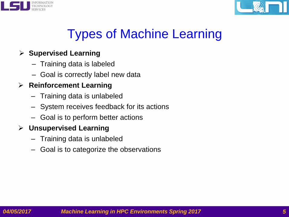
Types of Machine Learning
Supervised Learning
– Training data is labeled
– Goal is correctly label new data
Reinforcement Learning
– Training data is unlabeled
– System receives feedback for its actions
– Goal is to perform better actions
Unsupervised Learning
– Training data is unlabeled
– Goal is to categorize the observations
04/05/2017 Machine Learning in HPC Environments Spring 2017 5

Applications of Machine Learning
Handwriting Recognition
– convert written letters into digital letters
Language Translation
– translate spoken and or written languages (e.g. Google Translate)
Speech Recognition
– convert voice snippets to text (e.g. Siri, Cortana, and Alexa)
Image Classification
– label images with appropriate categories (e.g. Google Photos)
Autonomous Driving
– enable cars to drive
04/05/2017 Machine Learning in HPC Environments Spring 2017 6

Features in Machine Learning
Features are the observations that are used to form predictions
– For image classification, the pixels are the features
– For voice recognition, the pitch and volume of the sound samples are
the features
– For autonomous cars, data from the cameras, range sensors, and GPS
are features
Extracting relevant features is important for building a model
– Time of day is an irrelevant feature when classifying images
– Time of day is relevant when classifying emails because SPAM often
occurs at night
Common Types of Features in Robotics
– Pixels (RGB data)
– Depth data (sonar, laser rangefinders)
– Movement (encoder values)
– Orientation or Acceleration (Gyroscope, Accelerometer, Compass)
04/05/2017 Machine Learning in HPC Environments Spring 2017 7

Training and Test Data Training Data
– data used to learn a model
Test Data
– data used to assess the accuracy of model
Overfitting
– Model performs well on training data but poorly on test data
04/05/2017 Machine Learning in HPC Environments Spring 2017 8

Bias and Variance
Bias: expected difference between model’s prediction and truth
Variance: how much the model differs among training sets
Model Scenarios
– High Bias: Model makes inaccurate predictions on training data
– High Variance: Model does not generalize to new datasets
– Low Bias: Model makes accurate predictions on training data
– Low Variance: Model generalizes to new datasets
04/05/2017 Machine Learning in HPC Environments Spring 2017 9

Supervised Learning Algorithms
Linear Regression
Decision Trees
Support Vector Machines
K-Nearest Neighbor
Neural Networks
– Deep Learning is the branch of Machine Learning based on Deep
Neural Networks (DNNs, i.e., neural networks composed of more than 1
hidden layer).
– Convolutional Neural Networks (CNNs) are one of the most popular
DNN architectures (so CNNs are part of Deep Learning), but by no
means the only one.
04/05/2017 Machine Learning in HPC Environments Spring 2017 10

Machine Learning Frameworks
Tool Uses Language
Scikit-Learn Classification,
Regression, Clustering Python
Spark MLlib Classification,
Regression, Clustering Scala, R, Java
Weka Classification,
Regression, Clustering Java
Caffe Neural Networks C++, Python
TensorFlow Neural Networks Python
04/05/2017 Machine Learning in HPC Environments Spring 2017 11

Overview of LONI QB2
Deep Learning Examples on LONI QB2
04/05/2017 12

QB2 Hardware Specs
QB2 came on-line 5 Nov 2014.
– It is a 1.5 Petaflop peak performance cluster containing 504 compute
nodes with
• 960 NVIDIA Tesla K20x GPU's, and
• Over 10,000 Intel Xeon processing cores. It achieved 1.052 PF during
testing.
Ranked 46th on the November 2014 Top500 list.
480 Compute Nodes, each with:
– Two 10-core 2.8 GHz E5-2680v2 Xeon processors.
– 64 GB memory
– 500 GB HDD
– 2 NVIDIA Tesla K20x GPU's
04/05/2017 Machine Learning in HPC Environments Spring 2017 13

Inside A QB Cluster Rack
04/05/2017 Machine Learning in HPC Environments Spring 2017
Rack
Infiniband
Switch
Compute
Node
14

Inside A QB2 Dell C8000 Node
04/05/2017 Machine Learning in HPC Environments Spring 2017
Storage
Accelerator
(GPU) Accelerator
(GPU)
Processor
Memory
Network
Card
Processor
15

GPU CPU
Add GPUs: Accelerate Science Applications
Deep Learning Practice on LONI QB2 Fall 2016 11/09/2016 16

Performance Comparison
CPU-GPU Comparison of runtime for deep learning benchmark problem
– CIFAR10, 1 Epoch
11/09/2016 Deep Learning Practice on LONI QB2 Fall 2016
Speedups: 537/47=11.4 537/23=23.3
17
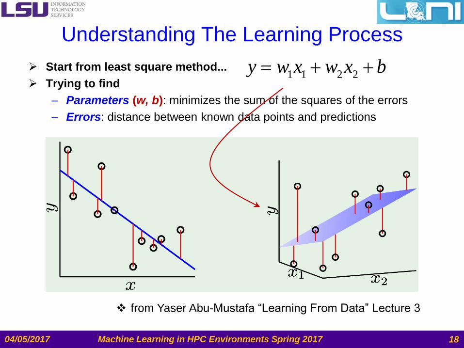
Understanding The Learning Process
Start from least square method...
Trying to find
– Parameters (w, b): minimizes the sum of the squares of the errors
– Errors: distance between known data points and predictions
04/05/2017 Machine Learning in HPC Environments Spring 2017 18
from Yaser Abu-Mustafa “Learning From Data” Lecture 3
1 1 2 2y w x w x b
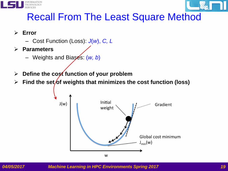
Recall From The Least Square Method
Error
– Cost Function (Loss): J(w), C, L
Parameters
– Weights and Biases: (w, b)
Define the cost function of your problem
Find the set of weights that minimizes the cost function (loss)
04/05/2017 Machine Learning in HPC Environments Spring 2017 19

Theory: Gradient Descent
Gradient descent is a first-order iterative optimization algorithm. To
find a local minimum of a function using gradient descent, one takes
steps proportional to the negative of the gradient (or of the
approximate gradient) of the function at the current point.
04/05/2017 Machine Learning in HPC Environments Spring 2017 20
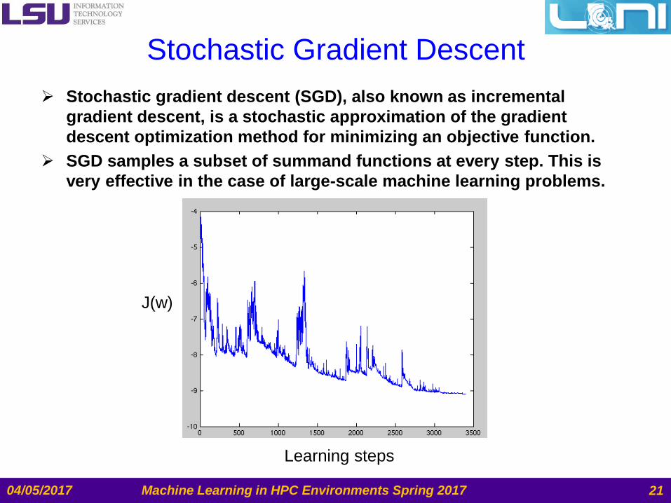
Stochastic Gradient Descent
Stochastic gradient descent (SGD), also known as incremental
gradient descent, is a stochastic approximation of the gradient
descent optimization method for minimizing an objective function.
SGD samples a subset of summand functions at every step. This is
very effective in the case of large-scale machine learning problems.
04/05/2017 Machine Learning in HPC Environments Spring 2017 21
J(w)
Learning steps

Mini-batch Gradient Descent
Batch gradient descent:
– Use all examples in each iteration
Stochastic gradient descent:
– Use one example in each iteration
Mini-batch gradient descent
– Use b examples in each iteration
In the neural network terminology:
– one EPOCH = one forward pass and one backward pass of all the
training examples
– batch size = the number of training examples in one forward/backward
pass. The higher the batch size, the more memory space you'll need.
– number of iterations = number of passes, each pass using [batch size]
number of examples. To be clear, one pass = one forward pass + one
backward pass (we do not count the forward pass and backward pass
as two different passes).
– Example: if you have 1000 training examples, and your batch size is
500, then it will take 2 iterations to complete 1 epoch.
04/05/2017 Machine Learning in HPC Environments Spring 2017 22

What is a neural network?
Start from a perceptron
04/05/2017 Machine Learning in HPC Environments Spring 2017 23
1 1 2 2 3 3( ) sign
sign
sign
i ii
T
h x w x w x w x b
w x b
b
w x
w1
w2
w3
b
x1
x2
x3
h(x)
+1
1
2
3
x
x
x
x
1
2
3
w
w
w
w
x1 age 23
x2 gender male
x3 annual salary $30,000
b threshold some value
h(x) Approve credit if: h(x)>0
Feature vector: x
Denote as: z
Hypothesis
(Prediction: y)
Weight vector: w
Activation function:
σ(z)=sign(z)

Perceptron To Neuron
Replace the sign to sigmoid
04/05/2017 Machine Learning in HPC Environments Spring 2017 24
1 1 2 2 3 3( ) sigmoid
sigmoid
sigmoid
i ii
T
h x w x w x w x b
w x b
b
w x
b
h(x)
Activation function:
σ(z)=sigmoid(z)
y h x z
Tz b w x1
2
3
x
x
x
x
1
2
3
w
w
w
w
Feature vector: x Weight vector: w
w1
w2
w3
x1
x2
x3
+1

Sigmoid Neurons
Sigmoid activation Function
– In the field of Artificial Neural Networks, the sigmoid function is a type of
activation function for artificial neurons.
There are many other activation functions used. (We will touch later.)
04/05/2017 Machine Learning in HPC Environments Spring 2017 25
1
1 zz
e
z sign z
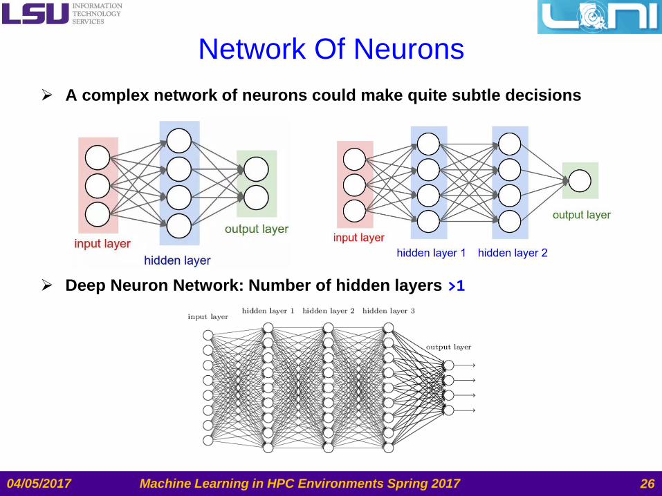
Network Of Neurons
A complex network of neurons could make quite subtle decisions
Deep Neuron Network: Number of hidden layers >1
04/05/2017 Machine Learning in HPC Environments Spring 2017 26

How to Train DNN?
Backward Propagation
– The backward propagation of errors or backpropagation, is a common
method of training artificial neural networks and used in conjunction with
an optimization method such as gradient descent.
Deep Neural Networks are hard to train
– learning machines with lots of (typically in range of million) parameters
– Unstable gradients issue
• Vanishing gradient problem
• Exploding gradient problem
– Choice of network architecture and other hyper-parameters is also
important.
– Many factors can play a role in making deep networks hard to train
– Understanding all those factors is still a subject of ongoing research
04/05/2017 Machine Learning in HPC Environments Spring 2017 27

Hello World of Deep Learning:
Recognition of MNIST
Deep Learning Example
04/05/2017 28

Introducing the MNIST problem
MNIST (Mixed National Institute of Standards and Technology
database) is a large database of handwritten digits that is commonly
used for training various image processing systems.
It consists of images of handwritten digits like these:
The MNIST database contains 60,000 training images and 10,000
testing images.
04/05/2017 29 Machine Learning in HPC Environments Spring 2017
Example Problem - MNIST
Recognizes handwritten digits.
We uses the MNIST dataset, a collection of 60,000 labeled digits that
has kept generations of PhDs busy for almost two decades. You will
solve the problem with less than 100 lines of
Python/Keras/TensorFlow code.
We will gradually enhance the neural network to achieve above 99%
accuracy by using the mentioned techniques.
04/05/2017 Machine Learning in HPC Environments Spring 2017 30

Steps for MNIST
Understand the MNIST data
Softmax regression layer
The cost function
04/05/2017 Machine Learning in HPC Environments Spring 2017 31

The MNIST Data
Every MNIST data point has two parts: an image of a handwritten digit
and a corresponding label. We'll call the images "x" and the labels "y".
Both the training set and test set contain images and their
corresponding labels;
Each image is 28 pixels by 28 pixels. We can interpret this as a big
array of numbers:
04/05/2017 Machine Learning in HPC Environments Spring 2017 32

One Layer NN for MNIST Recognition
We will start with a very simple model, called Softmax Regression.
We can flatten this array into a vector of 28x28 = 784 numbers. It
doesn't matter how we flatten the array, as long as we're consistent
between images.
From this perspective, the MNIST images are just a bunch of points in
a 784-dimensional vector space.
04/05/2017 Machine Learning in HPC Environments Spring 2017 33
...
28x28
pixels

Result of the Flatten Operation
The result is that the training images is a matrix (tensor) with a shape
of [60000, 784].
The first dimension is an index into the list of images and the second
dimension is the index for each pixel in each image.
Each entry in the tensor is a pixel intensity between 0 and 1, for a
particular pixel in a particular image.
04/05/2017 Machine Learning in HPC Environments Spring 2017 34
60000
60,000
784

One-hot Vector (One vs All)
For the purposes of this tutorial, we label the y’s as "one-hot vectors“.
A one-hot vector is a vector which is 0 in most dimensions, and 1 in a
single dimension.
How to label an “8”?
– [0,0,0,0,0,0,0,0,1,0]
What is the dimension of our y matrix (tensor)?
04/05/2017 Machine Learning in HPC Environments Spring 2017 35
60,000
10
0 0 0 0 0 0 1 0 0 0
0 0 0 1 0 0 0 0 0 0
0 0 1 0 0 0 0 0 0 0
0 0 0 0 1 0 0 0 0 0
0 0 0 0 0 1 0 0 0 0
0 0 0 0 1 0 0 0 0 0
...
0 0 0 0 1 0 0 0 0 0
6
3
2
4
5
4
...
4
60,000 labels:
0 1 2 3 4 5 6 7 8 9
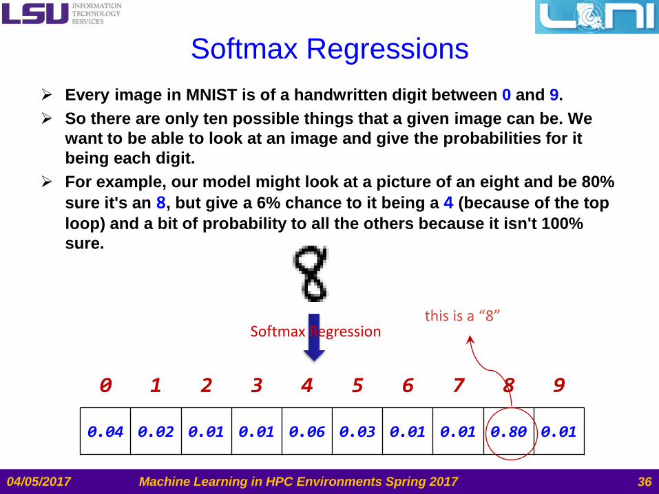
Softmax Regressions
Every image in MNIST is of a handwritten digit between 0 and 9.
So there are only ten possible things that a given image can be. We
want to be able to look at an image and give the probabilities for it
being each digit.
For example, our model might look at a picture of an eight and be 80%
sure it's an 8, but give a 6% chance to it being a 4 (because of the top
loop) and a bit of probability to all the others because it isn't 100%
sure.
04/05/2017 Machine Learning in HPC Environments Spring 2017 36
0 1 2 3 4 5 6 7 8 9
0.04 0.02 0.01 0.01 0.06 0.03 0.01 0.01 0.80 0.01
Softmax Regression this is a “8”

2 steps in softmax regression - Step 1
Step 1: Add up the evidence of our input being in certain classes.
– Do a weighted sum of the pixel intensities. The weight is negative if that
pixel having a high intensity is evidence against the image being in that
class, and positive if it is evidence in favor.
04/05/2017 Machine Learning in HPC Environments Spring 2017 37
,i i j j ijz W x b

Matrix Representation of softmax layer
04/05/2017 Machine Learning in HPC Environments Spring 2017 38
784 pixels
X : 60,000 images,
one per line,
flattened
w0,0 w0,1 w0,2 w0,3 … w0,9 w1,0 w1,1 w1,2 w1,3 … w1,9 w2,0 w2,1 w2,2 w2,3 … w2,9 w3,0 w3,1 w3,2 w3,3 … w3,9 w4,0 w4,1 w4,2 w4,3 … w4,9 w5,0 w5,1 w5,2 w5,3 … w5,9 w6,0 w6,1 w6,2 w6,3 … w6,9 w7,0 w7,1 w7,2 w7,3 … w7,9 w8,0 w8,1 w8,2 w8,3 … w8,9 … w783,0 w783,1 w783,2 … w783,9
78
4 lin
es
broadcast
10 columns
x x x x x x x
softmax( )Y X W b

2 steps in softmax regression - Step 2
Step 2: Convert the evidence tallies into our predicted probabilities y
using the "softmax" function:
Here softmax is serving as an "activation" function, shaping the
output of our linear function a probability distribution over 10 cases,
defined as:
04/05/2017 Machine Learning in HPC Environments Spring 2017 39
,softmax softmaxi i i j j ijh z W x b x
exp
softmax normalize expexp
i
i
jj
zz z
z

Softmax on a batch of images
More compact representation for “softmaxing” on all the images
04/05/2017 Machine Learning in HPC Environments Spring 2017 40
softmax( )Y X W b
Predictions Images Weights Biases
Y[60000, 10] [60000, 784] W[784,10] b[10]
matrix multiply broadcast
on all lines
applied on
each line
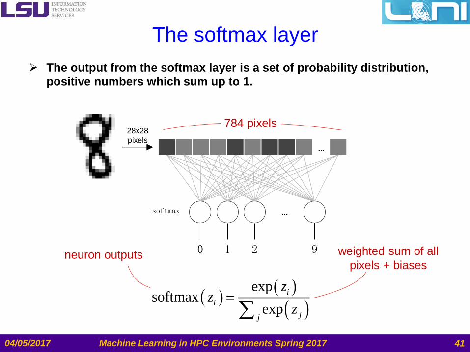
The softmax layer
The output from the softmax layer is a set of probability distribution,
positive numbers which sum up to 1.
04/05/2017 Machine Learning in HPC Environments Spring 2017
28x28
pixels
softmax
...
...
0 1 2 9
784 pixels
weighted sum of all
pixels + biases neuron outputs
41
exp
softmaxexp
i
i
jj
zz
z

0.01 0.01 0.01 0.01 0.01 0.01 0.90 0.01 0.02 0.01
The Cross-Entropy Cost Function
For classification problems, the Cross-Entropy cost function works
better than quadratic cost function.
We define the cross-entropy cost function for the neural network by:
04/05/2017 Machine Learning in HPC Environments Spring 2017
' 'logi iC y y
computed probabilities
this is a “6”
“one-hot” encoded ground truth
0 1 2 3 4 5 6 7 8 9
42
0 0 0 0 0 0 1 0 0 0
Cross entropy

Short Summary
How MNIST data is organized
– X:
• Flattened image pixels matrix
– Y:
• One-hot vector
Softmax regression layer
– Linear regression
– Output probability for each category
Cost function
– Cross-entropy
04/05/2017 Machine Learning in HPC Environments Spring 2017 43

Implementation in
Keras/Tensorflow
Deep Learning Example
04/05/2017 44 Machine Learning in HPC Environments Spring 2017
Few Words about
Keras, Tensorflow and Theano Keras is a high-level neural networks library, written in Python and
capable of running on top of either TensorFlow or Theano.
TensorFlow is an open source software library for numerical
computation using data flow graphs.
Theano is a Python library that allows you to define, optimize, and
evaluate mathematical expressions involving multi-dimensional arrays
efficiently.
04/05/2017 Machine Learning in HPC Environments Spring 2017 45

Introducing Keras
Keras is a high-level neural networks library,
Written in Python and capable of running on top of either TensorFlow
or Theano.
It was developed with a focus on enabling fast experimentation. Being
able to go from idea to result with the least possible delay is key to
doing good research.
See more at: https://github.com/fchollet/keras
04/05/2017 Machine Learning in HPC Environments Spring 2017 46

Typical Code Structure
Load the dataset (MNIST)
Build the Neural Network/Machine Learning Model
Train the model
04/05/2017 Machine Learning in HPC Environments Spring 2017 47

Software Environment
What you'll need
– Python 2 or 3 (Python 3 recommended)
– TensorFlow/Keras
– Matplotlib (Python visualization library)
On LONI QB2 the above modules are already setup for you, simply
use:
$ module load python/2.7.12-anaconda-tensorflow
OR
$ module load python/3.5.2-anaconda-tensorflow
04/05/2017 Machine Learning in HPC Environments Spring 2017 48

Keras - Initialization
# import necessary modules
from keras.models import Sequential
from keras.layers import Dense, Dropout, Activation, Flatten
from keras.layers import Convolution2D, MaxPooling2D
from keras.utils import np_utils
from keras import backend as K
04/05/2017 Machine Learning in HPC Environments Spring 2017 49

Load The MNIST Dataset
# load the mnist dataset
import cPickle
import gzip
f = gzip.open('mnist.pkl.gz', 'rb')
# load the training and test dataset
# download https://s3.amazonaws.com/img-datasets/mnist.pkl.gz
# to use in this tutorial
X_train, y_train, X_test, y_test = cPickle.load(f)
print(X_train.shape, y_train.shape, X_test.shape, y_test.shape)
Output of the print line:
(60000, 28, 28) (60000,) (10000, 28, 28) (10000,)
04/05/2017 Machine Learning in HPC Environments Spring 2017 50

Preprocessing the MNIST Dataset
# Flatten the image to 1D
X_train = X_train.reshape(X_train.shape[0], img_rows*img_cols)
X_test = X_test.reshape(X_test.shape[0], img_rows*img_cols)
input_shape = (img_rows*img_cols,)
# convert all data to 0.0-1.0 float values
X_train = X_train.astype('float32')
X_test = X_test.astype('float32')
X_train /= 255
X_test /= 255
# convert class vectors to binary class matrices
Y_train = np_utils.to_categorical(y_train, nb_classes)
Y_test = np_utils.to_categorical(y_test, nb_classes)
04/05/2017 Machine Learning in HPC Environments Spring 2017 51
One-hot encoding
All grayscale values to 0.0-1.0
Flatten 28x28 image to 1D

Build The First softmax Layer
# The Sequential model is a linear stack of layers in Keras
model = Sequential()
#build the softmax regression layer
model.add(Dense(nb_classes,input_shape=input_shape))
model.add(Activation('softmax'))
# Before training a model,
# configure the learning process via the compile method.
# using the cross-entropy loss function (objective)
model.compile(loss='categorical_crossentropy',
#using the stochastic gradient descent (SGD)
optimizer='sgd',
# using accuracy to judge the performance of your model
metrics=['accuracy'])
# fit the model, the training process
h = model.fit(X_train, Y_train, batch_size=batch_size, nb_epoch=nb_epoch,
verbose=1, validation_data=(X_test, Y_test))
04/05/2017 Machine Learning in HPC Environments Spring 2017 52
nb_classes=10 input_shape=(784,)

Results Of The First softmax Regression
Training accuracy vs Test accuracy, loss function
We reach a Training accuracy at 91.7%
04/05/2017 Machine Learning in HPC Environments Spring 2017 53
91.70%
test accuracy
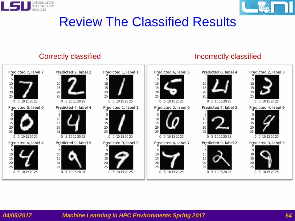
Review The Classified Results
04/05/2017 Machine Learning in HPC Environments Spring 2017 54
Correctly classified Incorrectly classified

Adding More Layers?
Using a 5 fully connected layer model:
04/05/2017 Machine Learning in HPC Environments Spring 2017 55
sigmoid
tanh
relu
0 1 2 ... 9
200
100
60
30
10 softmax
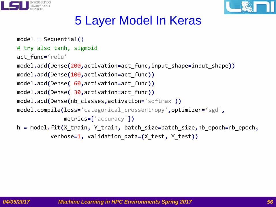
5 Layer Model In Keras
model = Sequential()
# try also tanh, sigmoid
act_func=‘relu'
model.add(Dense(200,activation=act_func,input_shape=input_shape))
model.add(Dense(100,activation=act_func))
model.add(Dense( 60,activation=act_func))
model.add(Dense( 30,activation=act_func))
model.add(Dense(nb_classes,activation='softmax'))
model.compile(loss='categorical_crossentropy',optimizer=‘sgd',
metrics=['accuracy'])
h = model.fit(X_train, Y_train, batch_size=batch_size,nb_epoch=nb_epoch,
verbose=1, validation_data=(X_test, Y_test))
04/05/2017 Machine Learning in HPC Environments Spring 2017 56

5 Layer Regression – Different Activation
Training accuracy vs Test accuracy, loss function
We reach a Test accuracy at 97.35% (sigmoid), 98.06% (tanh)
04/05/2017 Machine Learning in HPC Environments Spring 2017 57
sigmoid
tanh

Rectified Linear Unit (ReLU)
activation function ReLU - The Rectified Linear Unit has become very popular in the last
few years:
We get a test accuracy of 98.07% with ReLU
04/05/2017 Machine Learning in HPC Environments Spring 2017 58
relu
max 0,f z z
Overfitting

Overfitting
Overfitting occurs when a model is excessively complex, such as
having too many parameters relative to the number of observations. A
model that has been overfit has poor predictive performance, as it
overreacts to minor fluctuations in the training data.
04/05/2017 Machine Learning in HPC Environments Spring 2017 59
Regression:
Classification:

Regularization - Dropout
Dropout is an extremely effective, simple and recently introduced
regularization technique by Srivastava et al (2014).
While training, dropout is implemented by only keeping a neuron
active with some probability p (a hyperparameter), or setting it to zero
otherwise.
It is quite simple to apply dropout in Keras.
# apply a dropout rate 0.25 (drop 25% of the neurons)
model.add(Dropout(0.25))
04/05/2017 Machine Learning in HPC Environments Spring 2017 60

Apply Dropout To The 5 Layer NN
model = Sequential()
act_func='relu'
p_dropout=0.25 # apply a dropout rate 25 %
model.add(Dense(200,activation=act_func,input_shape=input_shape))
model.add(Dropout(p_dropout))
model.add(Dense(100,activation=act_func))
model.add(Dropout(p_dropout))
model.add(Dense( 60,activation=act_func))
model.add(Dropout(p_dropout))
model.add(Dense( 30,activation=act_func))
model.add(Dropout(p_dropout))
model.add(Dense(nb_classes,activation='softmax'))
model.compile(loss='categorical_crossentropy',optimizer=‘sgd',
metrics=['accuracy'])
h = model.fit(X_train, Y_train, batch_size=batch_size,nb_epoch=nb_epoch,
verbose=1, validation_data=(X_test, Y_test))
04/05/2017 Machine Learning in HPC Environments Spring 2017 61

Results Using p_dropout=0.25
Resolve the overfitting issue
Sustained 98.26% accuracy
04/05/2017 Machine Learning in HPC Environments Spring 2017 62
98.26%
test accuracy

Why Using Fully Connected Layers?
Such a network architecture does not take into account the spatial
structure of the images.
– For instance, it treats input pixels which are far apart and close together
on exactly the same weight.
Spatial structure must instead be inferred from the training data.
Is there an architecture which tries to take advantage of the spatial
structure?
04/05/2017 Machine Learning in HPC Environments Spring 2017 63

Convolution Neuron Network
(CNN)
Deep convolutional network is one of the most widely used types of
deep network.
In a layer of a convolutional network, one "neuron" does a weighted
sum of the pixels just above it, across a small region of the image
only. It then acts normally by adding a bias and feeding the result
through its activation function.
The big difference is that each neuron reuses the same weights
whereas in the fully-connected networks seen previously, each neuron
had its own set of weights.
04/05/2017 Machine Learning in HPC Environments Spring 2017 64
convolutional
subsampling
convolutional
subsampling
convolutional
subsampling
from Martin Görner Learn TensorFlow and deep learning, without a Ph.D

How Does CNN Work?
By sliding the patch of weights (filter) across the image in both
directions (a convolution) you obtain as many output values as there
were pixels in the image (some padding is necessary at the edges).
04/05/2017 Machine Learning in HPC Environments Spring 2017 65
28
28
1
28x28x1 image
3x3x1 filter
convolve (slide) over all
spatial locations
activation map
1
28
28

Three basic ideas about CNN
Local receptive fields
Shared weights and biases:
Pooling
04/05/2017 Machine Learning in HPC Environments Spring 2017 66

Pooling Layer
Convolutional neural networks also contain pooling layers. Pooling
layers are usually used immediately after convolutional layers.
What the pooling layers do is simplify the information in the output
from the convolutional layer.
We can think of max-pooling as a way for the network to ask whether a
given feature is found anywhere in a region of the image. It then
throws away the exact positional information.
04/05/2017 Machine Learning in HPC Environments Spring 2017 67

Convolutional Network With
Fully Connected Layers
04/05/2017 Machine Learning in HPC Environments Spring 2017 68
convolutional layer
32 output channels
convolutional layer
32 output channels
28x28x1
200
3x3x32
fully connected layer
softmax layer 10
3x3x32
32
32

Stacking And Chaining
Convolutional Layers in Keras model = Sequential()
# Adding the convulation layers
model.add(Convolution2D(nb_filters, kernel_size[0], kernel_size[1],
border_mode='valid',
input_shape=input_shape))
model.add(Activation('relu'))
model.add(Convolution2D(nb_filters, kernel_size[0], kernel_size[1]))
model.add(Activation('relu'))
model.add(MaxPooling2D(pool_size=pool_size))
model.add(Dropout(0.25))
# Fully connected layers
model.add(Flatten())
model.add(Dense(256,activation='relu'))
model.add(Dropout(0.25))
model.add(Dense(nb_classes,activation('softmax'))
model.compile(loss='categorical_crossentropy', optimizer='adadelta', metrics=['accuracy'])
h = model.fit(X_train, Y_train, batch_size=batch_size, nb_epoch=nb_epoch,
verbose=1,callbacks=[history], validation_data=(X_test, Y_test))
04/05/2017 Machine Learning in HPC Environments Spring 2017 69
nb_filters=32 kernel_size=(3,3)
input_shape=(28,28)

Challenging The 99% Testing Accuracy
By using the convolution layer and the fully connected layers, we
reach a test accuracy of 99.23%
04/05/2017 Machine Learning in HPC Environments Spring 2017 70
99.23%
test accuracy

Review The Classified Results of CNN
04/05/2017 Machine Learning in HPC Environments Spring 2017 71
Correctly classified Incorrectly classified

Feed More Data:
Using Expanded Dataset We can further increase the test accuracy by expanding the
mnist.pkl.gz dataset, reaching a nearly 99.6% test accuracy
04/05/2017 Machine Learning in HPC Environments Spring 2017 72
99.57%
test accuracy

Examples of Convolution NN
LeNet (1998)
AlexNet (2012)
GoogleLeNet (2014)
04/05/2017 Machine Learning in HPC Environments Spring 2017 73

Machine Learning Courses List
Machine Learning in Coursera
https://www.coursera.org/learn/machine-learning
Learning from Data (Caltech)
https://work.caltech.edu/telecourse.html
Convolutional Neural Networks for Visual Recognition
http://cs231n.github.io/
Deep Learning for Natural Language Processing
https://cs224d.stanford.edu/
04/05/2017 Machine Learning in HPC Environments Spring 2017 74

How To Run Multiple Tests For
Hyper-parameters?
Machine Learning in HPC Environments
04/05/2017 75
Hyperparameters
Most machine learning algorithms involve “hyperparameters” which
are variables set before actually optimizing the model's parameters.
Setting the values of hyperparameters can be seen as model selection,
i.e. choosing which model to use from the hypothesized set of
possible models.
Examples of hyperparameters in Deep Neuron Network models:
– Number of Hidden Units
– Mini-batch Size
– Number of filters
– …
04/05/2017 76

Example Problem
I want to test which model works best if I have:
– 128, 256, 512 hidden units
– Mini-batch size=50, 100, 200
– Number of filters=8, 16, 32
Total 3x3=27 combinations
– Submit 27 jobs?
– Or we can do better?
04/05/2017 Machine Learning in HPC Environments Spring 2017 77

Usage of GNU Parallel
GNU parallel is a shell tool for executing jobs in parallel using one or
more computers (compute nodes).
A job can be a single command or a small script that has to be run for
each of the lines in the input.
The typical input is a list of files, a list of hosts, a list of users, a list of
URLs, or a list of tables.
See more at: https://www.gnu.org/software/parallel/

GNU Parallel Example Script
#!/bin/bash
#PBS -l nodes=3:ppn=20
#PBS -l walltime=2:00:00
#PBS -q workq
#PBS -N MNST_HYPER
#-j oe
#PBS -A loni_loniadmin3
cd $PBS_O_WORKDIR
export KERAS_BACKEND=tensorflow
SECONDS=0
parallel --joblog logfile \
-j 1 \
--slf $PBS_NODEFILE \
--workdir $PBS_O_WORKDIR \
python mnist_hparam.py ::: 1 2 3 ::: 256 512 1024
echo took $SECONDS secs.
04/05/2017 Machine Learning in HPC Environments Spring 2017 79
specify a log file
One job per node
Use 3 nodes for the job for 9 tests
3 sets of convolution layers
3 numbers of hidden units

Waste
Load Balancing in GNU Parallel
GNU Parallel spawns the next job when one finishes - keeping the
nodes active and thus saving time.
11/02/2016 Distributed Workload with GNU Parallel 80
Job 1
Job 2
Job 3
Job 4
Job 5
Job 6
Job 7
Job 8
Job 9
Waste
Waste
Job 1 Job 2 Job 3
Job 4
Job 5 Job 6
Job 7
Job 8 Job 9
Waste
Without Load Balancing With Load Balancing
Cpu0 Cpu1 Cpu2 Cpu0 Cpu1 Cpu2
Execution Time

Submit and Monitor Your Jobs
Deep Learning Examples on LONI QB2
04/05/2017 81

Two Job Types
Interactive job
– Set up an interactive environment on compute nodes for users
• Advantage: can run programs interactively
• Disadvantage: must be present when the job starts
– Purpose: testing and debugging, compiling
• Do not run on the head node!!!
• Try not to run interactive jobs with large core count, which is a waste of
resources)
Batch job
– Executed without user intervention using a job script
• Advantage: the system takes care of everything
• Disadvantage: can only execute one sequence of commands which cannot
changed after submission
– Purpose: production run
04/05/2017 Machine Learning in HPC Environments Spring 2017 82

PBS Script (MNIST)
Tensorflow Backend #!/bin/bash
#PBS -l nodes=1:ppn=20
#PBS -l walltime=72:00:00
#PBS -q workq
#PBS -N cnn.tf.gpu
#PBS -o cnn.tf.gpu.out
#PBS -e cnn.tf.gpu.err
#PBS -A loni_loniadmin1
cd $PBS_O_WORKDIR
# use the tensorflow backend
export KERAS_BACKEND=tensorflow
# use this python module key to access tensorflow, theano and keras
module load python/2.7.12-anaconda
python mnist_cnn.py
04/05/2017 Machine Learning in HPC Environments Spring 2017
Tells the job
scheduler
how much
resource you
need.
How will you
use the
resources?
83
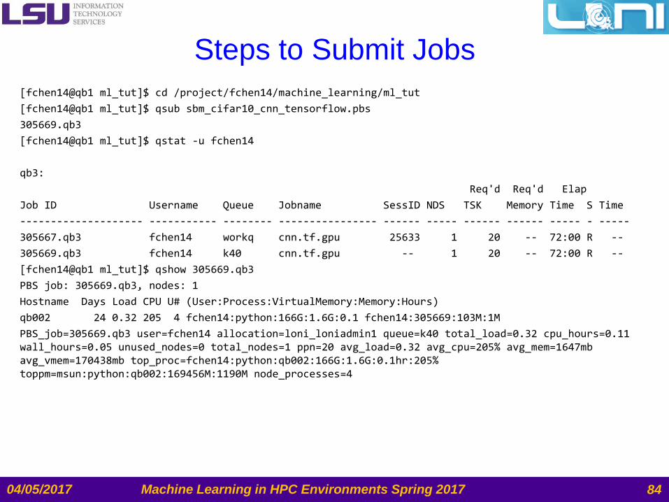
Steps to Submit Jobs
[fchen14@qb1 ml_tut]$ cd /project/fchen14/machine_learning/ml_tut
[fchen14@qb1 ml_tut]$ qsub sbm_cifar10_cnn_tensorflow.pbs
305669.qb3
[fchen14@qb1 ml_tut]$ qstat -u fchen14
qb3:
Req'd Req'd Elap
Job ID Username Queue Jobname SessID NDS TSK Memory Time S Time
-------------------- ----------- -------- ---------------- ------ ----- ------ ------ ----- - -----
305667.qb3 fchen14 workq cnn.tf.gpu 25633 1 20 -- 72:00 R --
305669.qb3 fchen14 k40 cnn.tf.gpu -- 1 20 -- 72:00 R --
[fchen14@qb1 ml_tut]$ qshow 305669.qb3
PBS job: 305669.qb3, nodes: 1
Hostname Days Load CPU U# (User:Process:VirtualMemory:Memory:Hours)
qb002 24 0.32 205 4 fchen14:python:166G:1.6G:0.1 fchen14:305669:103M:1M
PBS_job=305669.qb3 user=fchen14 allocation=loni_loniadmin1 queue=k40 total_load=0.32 cpu_hours=0.11 wall_hours=0.05 unused_nodes=0 total_nodes=1 ppn=20 avg_load=0.32 avg_cpu=205% avg_mem=1647mb avg_vmem=170438mb top_proc=fchen14:python:qb002:166G:1.6G:0.1hr:205% toppm=msun:python:qb002:169456M:1190M node_processes=4
04/05/2017 Machine Learning in HPC Environments Spring 2017 84

Job Monitoring - Linux Clusters
Check details on your job using qstat
$ qstat -n -u $USER : For quick look at nodes assigned to you
$ qstat -f jobid : For details on your job
$ qdel jobid : To delete job
Check approximate start time using showstart
$ showstart jobid
Check details of your job using checkjob
$ checkjob jobid
Check health of your job using qshow
$ qshow jobid
Dynamically monitor node status using top
– See next slides
Monitor GPU usage using nvidia-smi
– See next slides
Please pay close attention to the load and the memory consumed by
your job!
04/05/2017 Machine Learning in HPC Environments Spring 2017 85

Using the “top” command
The top program provides a dynamic real-time view of a running
system. [fchen14@qb1 ml_tut]$ ssh qb002
Last login: Mon Oct 17 22:50:16 2016 from qb1.loni.org
[fchen14@qb002 ~]$ top
top - 15:57:04 up 24 days, 5:38, 1 user, load average: 0.44, 0.48, 0.57
Tasks: 606 total, 1 running, 605 sleeping, 0 stopped, 0 zombie
Cpu(s): 9.0%us, 0.8%sy, 0.0%ni, 90.2%id, 0.0%wa, 0.0%hi, 0.0%si, 0.0%st
Mem: 132064556k total, 9759836k used, 122304720k free, 177272k buffers
Swap: 134217720k total, 0k used, 134217720k free, 5023172k cached
PID USER PR NI VIRT RES SHR S %CPU %MEM TIME+ COMMAND
21270 fchen14 20 0 166g 1.6g 237m S 203.6 1.3 16:42.05 python
22143 fchen14 20 0 26328 1764 1020 R 0.7 0.0 0:00.76 top
83 root 20 0 0 0 0 S 0.3 0.0 16:47.34 events/0
97 root 20 0 0 0 0 S 0.3 0.0 0:25.80 events/14
294 root 39 19 0 0 0 S 0.3 0.0 59:45.52 kipmi0
1 root 20 0 21432 1572 1256 S 0.0 0.0 0:01.50 init
2 root 20 0 0 0 0 S 0.0 0.0 0:00.02 kthreadd
04/05/2017 Machine Learning in HPC Environments Spring 2017 86

Monitor GPU Usage
Use nvidia-smi to monitor GPU usage: [fchen14@qb002 ~]$ nvidia-smi -l
Thu Nov 3 15:58:52 2016
+------------------------------------------------------+
| NVIDIA-SMI 352.93 Driver Version: 352.93 |
|-------------------------------+----------------------+----------------------+
| GPU Name Persistence-M| Bus-Id Disp.A | Volatile Uncorr. ECC |
| Fan Temp Perf Pwr:Usage/Cap| Memory-Usage | GPU-Util Compute M. |
|===============================+======================+======================|
| 0 Tesla K40m On | 0000:03:00.0 Off | 0 |
| N/A 34C P0 104W / 235W | 11011MiB / 11519MiB | 77% Default |
+-------------------------------+----------------------+----------------------+
| 1 Tesla K40m On | 0000:83:00.0 Off | 0 |
| N/A 32C P0 61W / 235W | 10950MiB / 11519MiB | 0% Default |
+-------------------------------+----------------------+----------------------+
+-----------------------------------------------------------------------------+
| Processes: GPU Memory |
| GPU PID Type Process name Usage |
|=============================================================================|
| 0 21270 C python 10954MiB |
| 1 21270 C python 10893MiB |
+-----------------------------------------------------------------------------+
04/05/2017 Machine Learning in HPC Environments Spring 2017 87

Future Trainings
This is the last training for this semester
– Keep an eye on future HPC trainings at:
• http://www.hpc.lsu.edu/training/tutorials.php#upcoming
Programming/Parallel Programming workshops in Summer
Visit our webpage: www.hpc.lsu.edu
04/05/2017 Machine Learning in HPC Environments Spring 2017 88