introduction to linear logic - brics · formulation of classical logic can be obtained by leaving...

BR

ICS

LS-96-6

T.Brauner:

Introductionto

LinearLogic

BRICSBasic Research in Computer Science

Introduction to Linear Logic

Torben Brauner

BRICS Lecture Series LS-96-6

ISSN 1395-2048 December 1996

Copyright c© 1996, BRICS, Department of Computer ScienceUniversity of Aarhus. All rights reserved.

Reproduction of all or part of this workis permitted for educational or research useon condition that this copyright notice isincluded in any copy.

See back inner page for a list of recent publications in the BRICSLecture Series. Copies may be obtained by contacting:

BRICSDepartment of Computer ScienceUniversity of AarhusNy Munkegade, building 540DK - 8000 Aarhus CDenmark

Telephone: +45 8942 3360Telefax: +45 8942 3255Internet: [email protected]

BRICS publications are in general accessible through World WideWeb and anonymous FTP:

http://www.brics.dk/

ftp://ftp.brics.dk/

This document in subdirectoryLS/96/6/

Introduction to Linear Logic

Torben Brauner

Torben BraunerBRICS1

Department of Computer ScienceUniversity of Aarhus

Ny MunkegadeDK-8000 Aarhus C, Denmark

1Basic Research In Computer Science,Centre of the Danish National Research Foundation.

Preface

The main concern of this report is to give an introduction to Linear Logic.For pedagogical purposes we shall also have a look at Classical Logic as wellas Intuitionistic Logic. Linear Logic was introduced by J.-Y. Girard in 1987and it has attracted much attention from computer scientists, as it is a logicalway of coping with resources and resource control. The focus of this technicalreport will be on proof-theory and computational interpretation of proofs,that is, we will focus on the question of how to interpret proofs as programsand reduction (cut-elimination) as evaluation. We first introduce ClassicalLogic. This is the fundamental idea of the proofs-as-programs paradigm.Cut-elimination for Classical Logic is highly non-deterministic; it is shownhow this can be remedied either by moving to Intuitionistic Logic or to LinearLogic. In the case on Linear Logic we consider Intuitionistic Linear Logic aswell as Classical Linear Logic. Furthermore, we take a look at the GirardTranslation translating Intuitionistic Logic into Intuitionistic Linear Logic.Also, we give a brief introduction to some concrete models of IntuitionisticLinear Logic. No proofs will be given except that a proof of cut-eliminationfor the multiplicative fragment of Classical Linear Logic is included in anappendix.

Acknowledgements. Thanks for comments from the participants of theBRICS Mini-course corresponding to this technical report. The proof-rulesare produced using Paul Taylor’s macros.

v

Contents

Preface v

1 Classical and Intuitionistic Logic 11.1 Classical Logic . . . . . . . . . . . . . . . . . . . . . . . . . . 11.2 Intuitionistic Logic . . . . . . . . . . . . . . . . . . . . . . . . 51.3 The λ-Calculus . . . . . . . . . . . . . . . . . . . . . . . . . . 81.4 The Curry-Howard Isomorphism . . . . . . . . . . . . . . . . . 12

2 Linear Logic 142.1 Classical Linear Logic . . . . . . . . . . . . . . . . . . . . . . . 142.2 Intuitionistic Linear Logic . . . . . . . . . . . . . . . . . . . . 192.3 A Digression - Russell’s Paradox and Linear Logic . . . . . . . 232.4 The Linear λ-Calculus . . . . . . . . . . . . . . . . . . . . . . 272.5 The Curry-Howard Isomorphism . . . . . . . . . . . . . . . . . 312.6 The Girard Translation . . . . . . . . . . . . . . . . . . . . . . 322.7 Concrete Models . . . . . . . . . . . . . . . . . . . . . . . . . 35

A Logics 40A.1 Classical Logic . . . . . . . . . . . . . . . . . . . . . . . . . . 40A.2 Intuitionistic Logic . . . . . . . . . . . . . . . . . . . . . . . . 42A.3 Classical Linear Logic . . . . . . . . . . . . . . . . . . . . . . . 43A.4 Intuitionistic Linear Logic . . . . . . . . . . . . . . . . . . . . 45

B Cut-Elimination for Classical Linear Logic 46B.1 Some Preliminary Results . . . . . . . . . . . . . . . . . . . . 46B.2 Putting the Proof Together . . . . . . . . . . . . . . . . . . . 52

vii

Chapter 1

Classical and IntuitionisticLogic

This chapter introduces Classical Logic and Intuitionistic Logic. Also, theCurry-Howard interpretation of Intuitionistic Logic, the λ-calculus, is dealtwith.

1.1 Classical Logic

The presentation of Classical Logic given in this section is based on the book[GLT89]. Formulas of Classical Logic are given by the grammar

s ::= 1 | s ∧ s | 0 | s ∨ s | s⇒ s.

The meta-variables A,B,C range over formulae. Proof-rules for a Gentzenstyle presentation of the logic are given in Appendix A.1; they are used toderive sequents

A1, ..., An ` B1, ..., Bm.

Such a sequent amounts to the formula expressing that the conjunction ofA1, ..., An implies the disjunction of B1, ..., Bm. The meta-variables Γ,∆range over lists of formulae and π, τ range over derivations as well as proofs.The Γ and ∆ parts of a sequent Γ ` ∆ are called contexts . The presenceof contraction and weakening proof-rules allows us to consider the contextsof a sequent as sets of formulae rather than multisets of formulae, which is

1

Chapter 1. Classical and Intuitionistic Logic

a feature distinguishing Classical Logic and Intuitionistic Logic from LinearLogic. The Gentzen style proof-rules were originally introduced in [Gen34].This presentation is characterised by the presence of two different forms ofrules for each connective, depending on which side of the turnstile the in-volved connective is introduced. Note that in Appendix A.1 the rules thatintroduce a connective on the left hand side have been positioned in the lefthand side column, and similarly, the rules that introduce a connective on theright hand side have been positioned in the right hand side column. Notealso that the rules for conjunction are symmetric to those for disjunction.

In the system above, negation is defined as ¬A = A⇒ 0. An alternativeformulation of Classical Logic can be obtained by leaving out implicationand having negation as a builtin connective together with the proof-rules

Γ ` A,∆¬L

Γ,¬A ` ∆

Γ, A ` ∆¬R

Γ ` ¬A,∆

Implication is then defined as A ⇒ B = ¬A ∨ B. We would then have aperfectly symmetric system. However, we have chosen the system of Ap-pendix A.1 with the aim of making clear the connection to IntuitionisticLogic.

One of the most important properties of the proof-rules for Classical Logicis that the cut-rule is redundant; this was originally proved by Gentzen in[Gen34]. The idea is that an application of the cut rule can either be pushedupwards in the surrounding proof or it can be replaced by cuts involvingsimpler formulae. The latter situation amounts to the following key-cases inwhich the cut formula is introduced in the last used rules of both immediatesubproofs:

• The (∧R,∧L1) key-case

··· π1

Γ ` A,∆

··· π2

Γ′ ` B,∆′

Γ,Γ′ ` A ∧B,∆,∆′

··· π′1

Γ′′, A ` ∆′′

Γ′′, A ∧ B ` ∆′′

Γ′′,Γ,Γ′ ` ∆′′,∆,∆′

;

··· π1

Γ ` A,∆

··· π′1

Γ′′, A ` ∆′′

Γ′′,Γ ` ∆′′,∆================Γ′′,Γ,Γ′ ` ∆′′,∆′,∆

2

1.1. Classical Logic

• The (∧R,∧L2) key-case

··· π1

Γ ` A,∆

··· π2

Γ′ ` B,∆′

Γ,Γ′ ` A ∧ B,∆,∆′

··· π′1

Γ′′, B ` ∆′′

Γ′′, A ∧B ` ∆′′

Γ′′,Γ,Γ′ ` ∆′′,∆,∆′

;

··· π2

Γ′ ` B,∆′··· π′1

Γ′′, B ` ∆′′

Γ′′,Γ′ ` ∆′′,∆′

================Γ′′,Γ,Γ′ ` ∆′′,∆′,∆

• The (1R, 1L) key-case

` 1

··· π′1

Γ′ ` ∆′

Γ′, 1 ` ∆′

Γ′ ` ∆′

;

··· π′1

Γ′ ` ∆′

• The (⇒R,⇒L) key-case

··· π1

Γ, A ` B,∆Γ ` A⇒ B,∆

··· π′1

Γ′ ` A,∆′··· π′2

Γ′′, B ` ∆′′

Γ′,Γ′′, A⇒ B ` ∆′′,∆′

Γ′,Γ′′,Γ ` ∆′′,∆′,∆

;

··· π′1

Γ′ ` A,∆′

··· π1

Γ, A ` B,∆

··· π′2

Γ′′, B ` ∆′′

Γ′′,Γ, A ` ∆′′,∆

Γ′′,Γ,Γ′ ` ∆′′,∆,∆′

A double bar denotes a number of applications of rules. We also have(∨R1,∨L), (∨R2,∨L), and (0R, 0L) key-cases, but they are left out as they

3


are symmetric to the mentioned (∧R,∧L1), (∧R,∧L2), and (1R, 1L) cases, re-spectively. We omit the full cut-elimination proof here; the reader is referredto [GLT89] for the details. A notable feature of the system is that all formu-lae occuring in a cut-free proof are subformulae of the formulae occuring inthe end-sequent. This is called the subformula property.

The fundamental idea in the proofs-as-programs paradigm is to considera proof as a program and reduction of the proof (cut-elimination) as evalua-tion of the program. This makes it desirable that the same reduced proof isobtained independent of the choices of reductions. However, this is not pos-sible with Classical Logic where cut-elimination is highly non-deterministic,as pointed out in [GLT89]. The problem is witnessed by the proof

··· πΓ ` ∆

Γ ` A,∆

··· π′

Γ′ ` ∆′

Γ′, A ` ∆′

Γ′,Γ ` ∆′,∆

which, because of its symmetry, can be reduced to both of the proofs

··· πΓ ` ∆

==========Γ′,Γ ` ∆′,∆

··· π′

Γ′ ` ∆′

==========Γ′,Γ ` ∆′,∆

The example implies that Classical Logic as given above has no non-trivialsound denotational semantics; all proofs of a given sequent will simply havethe same denotation. This deficiency can be remedied by breaking the sym-metry; two ways of doing so can be pointed out:

• Each right hand side context is subject to the restriction that it hasto contain exactly one formula. This amounts to Intuitionistic Logicwhich will be dealt with in Section 1.2.

• Contraction and weakening is marked explicitly using additional modal-ities ! and ? on formulae. The !-modality corresponds to contractionand weakening on the left hand side, and similarly, the ?-modality cor-responds to contraction and weakening on the right hand side. Thisamounts to Classical Linear Logic which will be dealt with in Sec-tion 2.1.

4

1.2. Intuitionistic Logic

This dichotomy goes back to [GLT89]. Since the publication of this booka considerable amount of work has been devoted to giving Classical Logica constructive formulation in the sense that proofs can be considered asprograms. This has essentially been achieved by “decorating” formulas withinformation controlling the process of cut-elimination. The work of Parigot,[Par91, Par92], Ong, [Ong96] and Girard, [Gir91] seems especially promising.A notable feature of the latter paper is the presentation of a categorical modelof Classical Logic where A is not isomorphic to ¬¬A. Thus, the dichotomyabove should not be considered as excluding other solutions. The lesson tolearn is that constructiveness, in the sense that proofs can be considered asprograms, is not a property of certain logics, but rather a property of certainformulations of logics.

1.2 Intuitionistic Logic

The presentation of Intuitionistic Logic given in this section is based on thebook [GLT89]. Formulae of Intuitionistic Logic are the same as the formulaeof Classical Logic. The proof-rules of Intuitionistic Logic in Gentzen styleoccur as those of Classical Logic given in Appendix A.1 where ∨L is written

Γ, A ` C Γ′, B ` C∨L

Γ,Γ′, A ∨B ` C

and the remaining rules are subject to the restriction that each right handside context contains exactly one formula.

We shall here consider also an equivalent Natural Deduction presentationof Intuitionistic Logic which has cleaner dynamic properties than the pre-sentation in Gentzen style. Proof-rules for this formulation of the logic aregiven in Appendix A.2; they are used to derive sequents

A1, ..., An ` B.

The Natural Deduction style proof-rules were originally introduced by Gentzenin [Gen34] and later considered by Pravitz in [Pra65]. This style of presen-tation is characterised by the presence of two different forms of rules foreach connective, namely introduction and elimination rules. Note that inAppendix A.2 the introduction rules have been positioned in the left hand

5


side column, and the elimination rules have been positioned in the right handside column. Note also that the contraction and weakening proof-rules areexplicitly part of the Gentzen style formulation whereas they are admissiblein the Natural Deduction formulation.

A notable feature of Intuitionistic Logic is the so-called Brouwer-Heyting-Kolmogorov functional interpretation where formulae are interpreted by meansof their proofs:

• A proof of a conjunction A ∧ B consists of a proof of A together witha proof of B,

• a proof of an implication A ⇒ B is a function from proofs of A toproofs of B,

• a proof of a disjunction A ∨ B is either a proof of A or a proof ofB together with a specification of which of the disjuncts is actuallyproved.

The proof-rules for Intuitionistic Logic can then be considered as methods fordefining functions such that a proof of a sequent Γ ` B gives rise to a functionwhich assigns a proof of the formula B to a list of proofs proving the respectiveformulae in the context Γ. Note that tertium non datur, A ∨ ¬A, whichdistinguishes Classical Logic from Intuitionistic Logic, cannot be interpretedin this way. It turns out that the λ-calculus is an appropriate language forexpressing the Brouwer-Heyting-Kolmogorov interpretation. We shall comeback to the λ-calculus in the next section, and in Section 1.4 we will introducethe Curry-Howard isomorphism that makes explicit the relation between theλ-calculus and Intuitionistic Logic.

Now, a Natural Deduction proof may be rewritten into a simpler formusing a reduction rule. Reduction of a Natural Deduction proof correspondsto cut-eliminating in a Gentzen style formulation. The reduction rules areas follows:

6

1.2. Intuitionistic Logic

• The (∧I ,∧E1) case

···Γ ` A

···Γ ` B

Γ ` A ∧ BΓ ` A

;

···Γ ` A

• The (∧I ,∧E2) case

···Γ ` A

···Γ ` B

Γ ` A ∧ BΓ ` B

;

···Γ ` B

• The (⇒I ,⇒E) case

Γ, A,Λ ` A···

Γ, A ` BΓ ` A⇒ B

···Γ ` A

Γ ` B

;

···Γ,Λ ` A···

Γ ` B

• The (∨I1,∨E) case

···Γ ` A

Γ ` A ∨B

Γ, A,Λ ` A···

Γ, A ` C

Γ, B,∆ ` B···

Γ, B ` CΓ ` C

;

···Γ,Λ ` A···

Γ ` C

7


• The (∨I2,∨E) case

···Γ ` B

Γ ` A ∨ B

Γ, A,Λ ` A···

Γ, A ` C

Γ, B,∆ ` B···

Γ, B ` CΓ ` C

;

···Γ,∆ ` B···

Γ ` C

Note how a reduction rule removes a “detour” in the proof created by theintroduction of a connective immediately followed by its elimination.

The Natural Deduction presentation of Intuitionistic Logic satisfies theChurch-Rosser property which means that whenever a proof π reduces toπ′ as well as to π′′, there exists a proof π′′′ to which both of the proofs π′

and π′′ reduce, and moreover, it satisfies the strong normalisation propertywhich means that all reduction sequences originating from a given proof areof finite length. Church-Rosser and strong normalisation implies that anyproof π reduces to a unique proof with the property that no reductions canbe applied; this is called the normal form of π. Via the Curry-Howardisomorphism this corresponds to analogous results for reduction of terms ofthe λ-calculus which we will come back to in the next two sections.

1.3 The λ-Calculus

The presentation of the λ-calculus given in this section is based on the book[GLT89]. In the next section we shall see how the λ-calculus occurs as aCurry-Howard interpretation of Intuitionistic Logic. Note that we considerproducts and sums as part of the λ-calculus; this convention is not followedby all authors. Types of the λ-calculus are given by the grammar

s ::= 1 | s× s | s⇒ s | 0 | s+ s

8

1.3. The λ-Calculus

Figure 1.1: Type Assignment Rules for the λ-Calculus

x1 : A1, ..., xn : An ` xq : Aq

Γ ` true : 1

Γ ` u : A Γ ` v : B

Γ ` (u, v) : A× BΓ ` u : A× BΓ ` fst(u) : A

Γ ` u : A×BΓ ` snd(u) : B

Γ, x : A ` u : B

Γ ` λxA.u : A⇒ B

Γ ` f : A⇒ B Γ ` u : A

Γ ` fu : B

Γ ` w : 0

Γ ` falseC(w) : C

Γ ` u : A

Γ ` inlA+B(u) : A+B

Γ ` u : B

Γ ` inrA+B(u) : A+B

Γ ` w : A+B Γ, x : A ` u : C Γ, y : B ` v : C

Γ ` case w of inl(x).u |inr(y).v : C

and terms are given by the grammar

t ::= x |true | (t, t) | fst(t) | snd(t) |λxA.t | tt |falseC(t) | inlA+B(t) | inrA+B(t) | case t of inl(x).t|inr(y).t

9


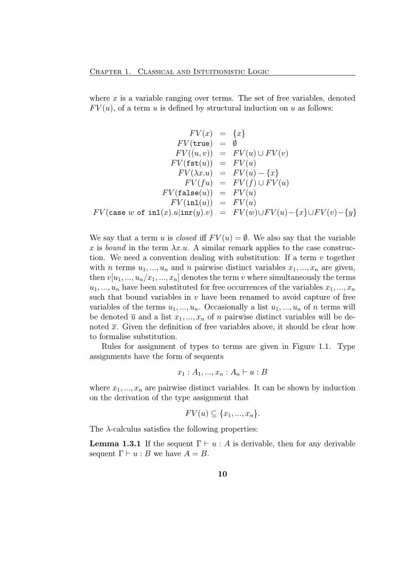
where x is a variable ranging over terms. The set of free variables, denotedFV (u), of a term u is defined by structural induction on u as follows:

FV (x) = {x}FV (true) = ∅FV ((u, v)) = FV (u) ∪ FV (v)FV (fst(u)) = FV (u)FV (λx.u) = FV (u)− {x}FV (fu) = FV (f) ∪ FV (u)

FV (false(u)) = FV (u)FV (inl(u)) = FV (u)

FV (case w of inl(x).u|inr(y).v) = FV (w)∪FV (u)−{x}∪FV (v)−{y}

We say that a term u is closed iff FV (u) = ∅. We also say that the variablex is bound in the term λx.u. A similar remark applies to the case construc-tion. We need a convention dealing with substitution: If a term v togetherwith n terms u1, ..., un and n pairwise distinct variables x1, ..., xn are given,then v[u1, ..., un/x1, ..., xn] denotes the term v where simultaneously the termsu1, ..., un have been substituted for free occurrences of the variables x1, ..., xnsuch that bound variables in v have been renamed to avoid capture of freevariables of the terms u1, ..., un. Occasionally a list u1, ..., un of n terms willbe denoted u and a list x1, ..., xn of n pairwise distinct variables will be de-noted x. Given the definition of free variables above, it should be clear howto formalise substitution.

Rules for assignment of types to terms are given in Figure 1.1. Typeassignments have the form of sequents

x1 : A1, ..., xn : An ` u : B

where x1, ..., xn are pairwise distinct variables. It can be shown by inductionon the derivation of the type assignment that

FV (u) ⊆ {x1, ..., xn}.

The λ-calculus satisfies the following properties:

Lemma 1.3.1 If the sequent Γ ` u : A is derivable, then for any derivablesequent Γ ` u : B we have A = B.

10

1.3. The λ-Calculus

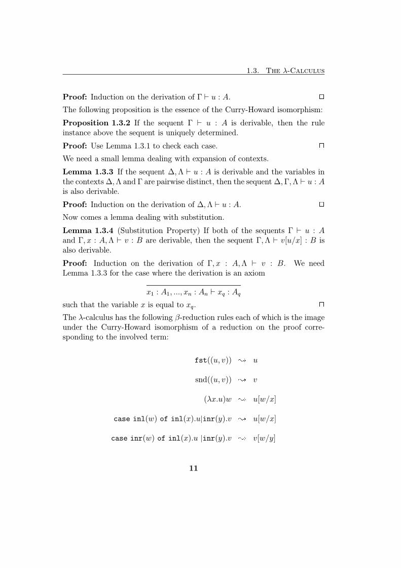
Proof: Induction on the derivation of Γ ` u : A. 2

The following proposition is the essence of the Curry-Howard isomorphism:

Proposition 1.3.2 If the sequent Γ ` u : A is derivable, then the ruleinstance above the sequent is uniquely determined.

Proof: Use Lemma 1.3.1 to check each case. 2

We need a small lemma dealing with expansion of contexts.

Lemma 1.3.3 If the sequent ∆,Λ ` u : A is derivable and the variables inthe contexts ∆,Λ and Γ are pairwise distinct, then the sequent ∆,Γ,Λ ` u : Ais also derivable.

Proof: Induction on the derivation of ∆,Λ ` u : A. 2

Now comes a lemma dealing with substitution.

Lemma 1.3.4 (Substitution Property) If both of the sequents Γ ` u : Aand Γ, x : A,Λ ` v : B are derivable, then the sequent Γ,Λ ` v[u/x] : B isalso derivable.

Proof: Induction on the derivation of Γ, x : A,Λ ` v : B. We needLemma 1.3.3 for the case where the derivation is an axiom

x1 : A1, ..., xn : An ` xq : Aq

such that the variable x is equal to xq. 2

The λ-calculus has the following β-reduction rules each of which is the imageunder the Curry-Howard isomorphism of a reduction on the proof corre-sponding to the involved term:

fst((u, v)) ; u

snd((u, v)) ; v

(λx.u)w ; u[w/x]

case inl(w) of inl(x).u|inr(y).v ; u[w/x]

case inr(w) of inl(x).u |inr(y).v ; v[w/y]

11


We shall not be concerned with η-reductions or commuting conversions. Theproperties of Church-Rosser and strong normalisation for proofs of Intuition-istic Logic correspond to analogous notions for terms of the λ-calculus viathe Curry-Howard isomorphism, and in [LS86] it is shown that these prop-erties are indeed satisfied. First strong normalisation is proved. By Konig’sLemma, this implies that any term t is bounded , that is, there exists a numbern such that no sequence of one-step reductions originating from t has morethan n steps. Given the result that all terms are bounded, Church-Rosser isproved by induction on the bound.

1.4 The Curry-Howard Isomorphism

The original Curry-Howard isomorphism, [How80], relates the Natural De-duction formulation of Intuitionistic Logic to the λ-calculus; formulae cor-respond to types, proofs to terms, and reduction of proofs to reduction ofterms. This is dealt with in [GLT89] and in [Abr90]; the first emphasises thelogic side of the isomorphism, the second the computational side. In whatfollows, we will consider the Natural Deduction presentation of IntuitionisticLogic given in Appendix A.2. The relation between formulae of IntuitionisticLogic and types of the λ-calculus is obvious. The idea of the Curry-Howardisomorphism on the level of proofs is that proof-rules can be “decorated”with terms such that the term induced by a proof encodes the proof. In thecase of Intuitionistic Logic an appropriate term language for this purposeis the λ-calculus. If we decorate the proof-rules of Intuitionistic Logic withterms in the appropriate way we get the rules for assigning types to termsof the λ-calculus, and moreover, if we take the typing rules of the λ-calculusand remove the variables and terms we can recover the proof-rules. We getthe Curry-Howard isomorphism on the level of proofs as follows: Given aproof of the sequent A1, ..., An ` B, that is, a proof of the formula B on as-sumptions A1, ..., An, one can inductively construct a derivation of a sequentx1 : A1, ..., xn : An ` u : B, that is, a term u of type B with free variablesx1, ..., x1 of respective types A1, ..., An. Conversely, if one has a derivablesequent x1 : A1, ..., xn : An ` u : B, there is an easy way of getting a proofof A1, ..., An ` B; erase all terms and variables in the derivation of the typeassignment. The two processes are each other’s inverses modulo renamingof variables. The isomorphism on the level of proofs is essentially given by

12

1.4. The Curry-Howard Isomorphism

Proposition 1.3.2.On the level of reduction the Curry-Howard isomorphism says that a re-

duction on a proof followed by application of the Curry-Howard isomorphismon the level of proofs, yields the same term as application of the Curry-Howard isomorphism on the level of proofs followed by the term-reductioncorresponding to the proof-reduction. This can be verified by applying theCurry-Howard isomorphism to the proofs involved in the reduction rules ofIntuitionistic Logic. For example, in the case of a (⇒I ,⇒E) reduction weget

Γ, x : A,Λ ` x : A···

Γ, x : A ` u : B

Γ ` λx.u : A⇒ B

···Γ ` v : A

Γ ` (λx.u)v : B

;

···Γ,Λ ` v : A

···Γ ` u[v/x] : B

We see that a β-reduction has taken place on the term encoding the proofon which the reduction is performed. In fact all β-reductions appear asCurry-Howard interpretations of reductions on the corresponding proofs.

13

Chapter 2

Linear Logic

This chapter introduces Classical Linear Logic and Intuitionistic Linear Logic.We make a detour to Russell’s Paradox with the aim of illustrating the dif-ference between Intuitionistic Logic and Intuitionistic Linear Logic. Also,the Curry-Howard interpretation of Intuitionistic Linear Logic, the linearλ-calculus, is dealt with. Furthermore, we take a look at the Girard Transla-tion translating Intuitionistic Logic into Intuitionistic Linear Logic. Finally,we give a brief introduction to some concrete models of Intuitionistic LinearLogic.

2.1 Classical Linear Logic

Linear Logic was discovered by J.-Y. Girard in 1987 and published in thenow famous paper [Gir87]. In the abstract of this paper, it is stated that“a completely new approach to the whole area between constructive logicsand computer science is initiated”. In [Gir89] the conceptual background ofLinear Logic is worked out. The fundamental idea of Linear Logic is to controlthe use of resources which is witnessed by the fact that the contraction andweakening proof-rules are not admissible in general. Rather, Linear Logicoccurs essentially as Classical Logic with the restriction that contractionand weakening is marked explicitly using additional modalities ! and ? onformulae. The !-modality corresponds to contraction and weakening on theleft hand side, and similarly, the ?-modality corresponds to contraction andweakening on the right hand side. A proof of !A amounts to having a proof

14

2.1. Classical Linear Logic

of A that can be used an arbitrary number of times.

Here we shall only consider the multiplicative fragment of Classical LinearLogic. Formulae are given by the grammar

s ::= I | s⊗ s | ⊥ | s............................................................................................... s | s( s | !s | ?s | & | 1 | ⊕ | 0.

Proof-rules for a Gentzen style presentation of the logic are given in Ap-pendix A.3; they are used to derive sequents

A1, ..., An−B1, ..., Bm.

A Girardian turnstile − is used to distinguish sequents of Classical LinearLogic from sequents of Classical Logic, where the usual turnstile ` is used.The &,1,⊕ and 0 connectives are called additive. The system obtained byexcluding the additives is called the multiplicative fragment. Note that, un-like most presentations of Classical Linear Logic, we use two-sided sequents,which will make the connection to Intuitionistic Linear Logic more explicit.Negation is then defined as A⊥ = A (⊥. The absence of contraction andweakening prevents us from considering the contexts of a sequent as sets offormulae, but we have to consider them to be multisets instead. This shouldbe compared to Classical and Intuitionistic Logic where we do have contrac-tion and weakening which implies that contexts can be considered as sets offormulae. The fact that contexts are considered as multisets means that ev-ery formula occuring in the context of a sequent has to be used exactly once.Therefore the two conjunctions & and ⊗ of Linear Logic are very differentconstructs: A proof of A&B consists of a proof of A together with a proofof B where exactly one of the proofs has to be used. A proof of A⊗ B alsoconsists of a proof of A together with a proof of B but here both of the proofshave to be used.

Now, as with Classical Logic, the cut-rule of Classical Linear Logic isredundant. Again the idea is that an application of the cut rule can eitherbe pushed upwards in the surrounding proof or it can be replaced by cutsinvolving simpler formulae. In Classical Linear Logic we have the followingkey-cases (excluding the additive key-cases which are similar to the corre-sponding key-cases for Classical Logic):

15

Chapter 2. Linear Logic

• The (⊗R,⊗L) key-case

··· π1

Γ ` A,∆

··· π2

Γ′ ` B,∆′

Γ,Γ′ ` A⊗ B,∆,∆′

··· π′1

Γ′′, A,B ` ∆′′

Γ′′, A⊗ B ` ∆′′

Γ′′,Γ,Γ′ ` ∆′′,∆,∆′

;

··· π1

Γ ` A,∆

··· π2

Γ′ ` B,∆′··· π′1

Γ′′, A,B ` ∆′′

Γ′′, A,Γ′ ` ∆′′,∆′

Γ′′,Γ,Γ′ ` ∆′′,∆′,∆

• The (IR, IL) key-case

` I

··· π′1

Γ′ ` ∆′

Γ′, I ` ∆′

Γ′ ` ∆′

;

··· π′1

Γ′ ` ∆′

16

2.1. Classical Linear Logic

• The ((R,(L) key-case

··· π1

Γ, A ` B,∆Γ ` A( B,∆

··· π′1

Γ′ ` A,∆′··· π′2

Γ′′, B ` ∆′′

Γ′,Γ′′, A( B ` ∆′′,∆′

Γ′,Γ′′,Γ ` ∆′′,∆′,∆

;

··· π′1

Γ′ ` A,∆′

··· π1

Γ, A ` B,∆

··· π′2

Γ′′, B ` ∆′′

Γ′′,Γ, A ` ∆′′,∆

Γ′′,Γ,Γ′ ` ∆′′,∆,∆′

• The (!R, !L) key-case

··· π1

!Γ ` A, ?∆

!Γ `!A, ?∆

··· π′1

Γ′, A ` ∆′

Γ′, !A ` ∆′

Γ′, !Γ ` ∆′, ?∆

;

··· π1

!Γ ` A, ?∆

··· π′1

Γ′, A ` ∆′

Γ′, !Γ ` ∆′, ?∆

• The (!R,WL) key-case

··· π1

!Γ ` A, ?∆

!Γ `!A, ?∆

··· π′1

Γ′ ` ∆′

Γ′, !A ` ∆′

Γ′, !Γ ` ∆′, ?∆

;

··· π′1

Γ′ ` ∆′

===========Γ′, !Γ ` ∆′, ?∆

We also have (...............................................................................................R,

...............................................................................................L), (⊥R,⊥L), (WR, ?L), and (?R, ?L) key-cases, but they

are left out as they are symmetric to the mentioned (⊗R,⊗L), (IR, IL),

17


(!R,WL), and (!R, !L) cases, respectively. The key-cases have the propertythat a cut is replaced by cuts involving simpler formulas. Furthermore wehave the following so-called pseudo key-case:

• The (!R, CL) pseudo key-case

··· π1

!Γ ` A, ?∆

!Γ `!A, ?∆

··· π′1

Γ′, !A, !A ` ∆′

Γ′, !A ` ∆′

Γ′, !Γ ` ∆′, ?∆

;

··· π1

!Γ ` A, ?∆

!Γ `!A, ?∆

··· π1

!Γ ` A, ?∆

!Γ `!A, ?∆

··· π′1

Γ′, !A, !A ` ∆′

Γ′, !Γ, !A ` ∆′, ?∆

Γ′, !Γ, !Γ ` ∆′, ?∆, ?∆=================

Γ′, !Γ ` ∆′, ?∆

We also have a (CR, ?L) pseudo key-case, but this is left out as it is symmetricto the mentioned (!R, CL) case. Note that in a pseudo key-case the cutformula is replaced by cuts involving the same formula. Hence, the pseudokey-cases does not simplify the involved cut formulas, which distinguishesthem from the key-cases (and this is indeed the reason why we call thempseudo key-cases). In Appendix B we shall give a proof of cut-eliminationfor the multiplicative fragment. As with Classical Logic, it is the case thatClassical Linear Logic satisfies the subformula property, that is, all formulaeoccuring in a cut-free proof are subformulae of the formulae occuring in theend-sequent.

Classical Linear Logic does not satisfy Church-Rosser, but on the otherhand, it is possible to give a non-trivial sound denotational semantics usingcoherence spaces, see [GLT89]. Thus, the non-determinism of cut-elimination

18

2.2. Intuitionistic Linear Logic

for Classical Linear Logic is limited. Note also that the example of Section 1.1showing the non-determinism of cut-elimination for Classical Logic does notgo through for Classical Linear Logic. It is, however, the case that themultiplicative fragment of Classical Linear Logic satisfies Church-Rosser, cf.[Laf96]. A proof can be found in [Dan90].

2.2 Intuitionistic Linear Logic

This section deals with Intuitionistic Linear Logic. The formulae are the sameas with Classical Linear Logic except that those involving the connectives⊥,..

............................................................................................. and ? are omitted. The proof-rules of Intuitionistic Linear Logic in

Gentzen style occur as those of Classical Linear Logic given in Appendix A.3where the proof-rules are subject to the restriction that each right hand sidecontext contains exactly one formula. It is possible to deal with the ⊥,.

..............................................................................................

and ? connectives intuitionistically by allowing sequents to have more thanone conclusion together with an appropriate restriction on the (R rule -see [BdP96, HdP93]. It turns out that the ! modality enables IntuitionisticLogic to be interpreted faithfully in Intuitionistic Linear Logic via the GirardTranslation - see Section 2.6.

Here we shall also consider a Natural Deduction presentation of Intu-itionistic Linear Logic which is equivalent to the Gentzen style formulation.Proof-rules for this formulation of the logic are given in Appendix A.4; theyare used to derive sequents

A1, ..., An−B.

The Natural Deduction presentation is the same as the one given in the paper[BBdPH92], and later fleshed out in detail in [Bie94]. A historical accountof the Natural Deduction presentation of Intuitionistic Linear Logic can befound in Section 4.4 of [Bra96].

As in Intuitionistic Logic, a proof might be rewritten into a simpler formusing a reduction rule. Again, reduction of a Natural Deduction proof cor-responds to cut-eliminating in a Gentzen style formulation. The reductionrules of the Natural Deduction presentation of Intuitionistic Linear Logicgiven here are as follows (excluding the additive reductions which are similarto the corresponding reductions for Intuitionistic Logic):

19


• The (II , IE) case

− I

···Γ−A

Γ−A

;

···Γ−A

• The (⊗I ,⊗E) case

···Γ−A

···∆−B

Γ,∆−A⊗B

A−A B−B···Λ, A,B−C

Λ,Γ,∆−C

;

···Γ−A

···∆−B···

Λ,Γ,∆−C

• The ((I ,(E) case

A−A···Γ, A−B

Γ−A( B

···Λ−A

Γ,Λ−B

;

···Λ−A···

Γ,Λ−B

20

2.2. Intuitionistic Linear Logic

• The (Promotion,Dereliction) case

···Γ1− !A1 , ... ,

···Γn− !An

!A1− !A1 , ..., !An− !An···!A1, ..., !An−B

Γ1, ...,Γn− !B

Γ1, ...,Γn−B

;

···Γ1− !A1 , ...,

···Γn− !An···

Γ1, ...,Γn−B

21


• The (Promotion, Contraction) case

···Γ1− !A1 , ...,

···Γn− !An

!A1− !A1 , ..., !An− !An···!A1, ..., !An−B

Γ1, ...,Γn− !B

!B− !B !B− !B···Λ, !B, !B−C

Λ,Γ1, ...,Γn−C

;

···Γ1− !A1 , ...,

···Γn− !An

!A1− !A1 , ..., !An− !An···!A1, ..., !An−B!A1, ..., !An− !B

!A1− !A1 , ..., !An− !An···!A1, ..., !An−B!A1, ..., !An− !B

···Λ, !A1, ..., !An, !A1, ..., !An−C

Λ,Γ1, ...,Γn−C

where the last used rule is derivable by using the Contraction andExchange rules. Note that a special case of the Contraction rule isused.

22

2.3. A Digression - Russell’s Paradox and Linear Logic

• The (Promotion,Weakening) case

···Γ1− !A1 , ... ,

···Γn− !An

!A1− !A1 , ..., !An− !An···!A1, ..., !An−B

Γ1, ...,Γn− !B Λ−CΛ,Γ1, ...,Γn−C

;

···Γ1− !A1 , ... ,

···Γn− !An Λ−C

Λ,Γ1, ...,Γn−C

where the last used rule is derivable by using the Weakening rule.

If we think of the Promotion rule as putting a “box” around the righthand side proof, then (Promotion,Dereliction) reduction removes the box,whereas the (Promotion, Contraction) and (Promotion,Weakening) reduc-tions respectively copy and discard the box.

Notions of Church-Rosser and strong normalisation for the Natural De-duction presentation of Intuitionistic Linear Logic are defined in analogywith the notions of Church-Rosser and strong normalisation for Intuitionis-tic Logic. Intuitionistic Linear Logic does indeed satisfy these properties; viaa Curry-Howard isomorphism this corresponds to analogous results for reduc-tion of terms of the linear λ-calculus which we will return to in Section 2.4and Section 2.5.

2.3 A Digression - Russell’s Paradox and

Linear Logic

In this section we will make a digression with the aim of illustrating the finegrained character of Intuitionistic Linear Logic compared to Intuitionistic

23


Logic. We will take set-theoretic comprehension into account: In both of thelogics unrestricted comprehension enables a contradiction to be proved viaRussell’s Paradox, but it turns out that Intuitionistic Linear Logic allows thepresence of a restricted form of comprehension, which is not possible in thecase of Intuitionistic Logic.

Unrestricted comprehension says that for any predicate A(x) there is aset {x |A(x)} with the property that

t ∈ {x |A(x)} ⇔ A(t).

This is a very strong axiom; it has all the axioms of Zermelo-Fraenkel settheory except the Axiom of Choice as special cases. An informal proof ofRussell’s Paradox now goes as follows: Using comprehension we define a setu as

u = {x | ¬(x ∈ x)}.Thus, u is the famous set of all those sets that are not elements of themselves.We then define a formula R to be

u ∈ u.

We then have R⇔ ¬R which enables a contradiction to be proved as follows:Assume R, this entails ¬R, which together with R entails a contradiction.Thus we have proved ¬R. The proof of ¬R also gives a proof of R. But aproof of ¬R together with a proof of R entails a contradiction.

Note how the contradiction is proved in two stages: First a formula Rsuch that R⇔ ¬R is defined, then a contradiction is derived in a proof wherethe assumption R is used twice. The two applications of the assumption Rare emphasised in the informal proof above. The are two ways of remedyingthis inconsistency:

• Unrestricted comprehension is replaced by weaker axioms such that itis impossible to define the set u and hence the formula R with theproperty that R ⇔ ¬R cannot be defined either. This was the optiontaken historically and which gave rise to Zermelo-Fraenkel set theory.

• Unrestricted comprehension is kept but the surrounding logic is weak-ened such that the existence of a formula R with the property thatR⇔ ¬R does not imply a contradiction. The !-free fragment of Linear

24

2.3. A Digression - Russell’s Paradox and Linear Logic

Logic is one such option as assumptions here can be used only once(recall that in deriving a contradiction from R ⇔ ¬R the assumptionR is used twice).

We will now flesh out some details of the second option. First we give a formalproof of Russell’s Paradox in Intuitionistic Logic extended with unrestrictedcomprehension as prescribed in [Pra65]. Recall that in Intuitionistic Logicnegation ¬A is defined as A⇒ 0. The grammar for formulae of IntuitionisticLogic is extended with an additional clause

s ::= ... | t ∈ t

and a grammar for terms is added

t ::= x | {x | s}

where x is a variable ranging over terms. Terms are to be thought of as sets(they should not be confused with terms of the λ-calculus). Furthermore,proof-rules for introduction and elimination of the connective ∈ are added

Γ ` A[t/x]∈I

Γ ` t ∈ {x |A}Γ ` t ∈ {x |A}

∈EΓ ` A[t/x]

The first stage of Russell’s Paradox is formalised as follows: We define theterm u and the formula R as above and get

Γ ` RΓ ` ¬R

and vice versa, which is equivalent to provability of ` R ⇒ ¬R and viceversa. The second stage of the paradox is formalised as follows: Two copiesof the proof

R ` RR ` ¬R R ` R

R,R ` 0

R ` 0

` ¬R

25


are applied in the proof···

` ¬R` R

···` ¬R

` 0

of a contradiction. Note that we have used the admissible contraction proof-rule together with a multiplicative version of the ⇒E rule which is also ad-missible in Intuitionistic Logic. The presence of contraction is crucial for theproof of inconsistency to go through. In [Pra65] the following observationis made: It can be shown that the sequent ` 0 is not provable by a normalproof; this means that no reduction sequences originating from the proof of` 0 above end in a normal proof. Indeed, the proof reduces in two stages toitself by carrying out the only performable reductions.

Now, above we have shown that unrestricted comprehension in the con-text of Intuitionistic Logic is inconsistent. But it turns out that we do not getinconsistency if we extend the !-free fragment of Intuitionistic Linear Logicwith unrestricted comprehension as above. Negation ¬A is here defined asA( 01. We still have a formula R such that R( ¬R and vice versa, butnow we cannot prove − 0 as before because contraction is forbidden. Thesystem was proved consistent in [Gri82] using the following two observations:A proof essentially shrinks under normalisation and there is no normal proofof − 0. The !-free fragment of Intuitionistic Linear Logic with unrestrictedcomprehension is, however, very unexpressive. A partial solution to this lackof expressiveness is to extend Intuitionistic Linear Logic with comprehensionas above but with the restriction that the ! modality is not allowed to occur inthe involved formula A(t). We still have the formula R such that R( ¬Rand vice versa, but it turns out that this system is consistent, which wasproved in [Shi94].

Hence, the fine-grainedness of Intuitionistic Linear Logic allows the pres-ence of a restricted form of comprehension, which is not possible in thecontext of Intuitionistic Logic. It should be mentioned that considerationson Russell’s Paradox in the context of Linear Logic have been crucial forGirard’s discovery of Light Linear Logic - see [Gir94].

1This is not the same as the negation A⊥ of Classical Linear Logic which is defined asA⊥ = A(⊥. However, this difference is not of importance here.

26

2.4. The Linear λ-Calculus

2.4 The Linear λ-Calculus

The presentation of the linear λ-calculus which we give in this section isthe same as the one given in [BBdPH92, BBdPH93], and later fleshed out indetail in [Bie94]. We have omitted the additive fragment as it is similar to thecorresponding fragment of the λ-calculus. The next section shows how thelinear λ-calculus occurs as a Curry-Howard interpretation of IntuitionisticLinear Logic in the same way as the λ-calculus occurs as a Curry-Howardinterpretation of Intuitionistic Logic. Types of the linear λ-calculus are givenby the grammar

s ::= I | s⊗ s | s( s | !s

and terms are given by the grammar

t ::= x |∗ | let t be ∗ in t | t⊗ t | let t be x⊗ y in t |λxA.t | tt |promote t, ..., t for x1, ..., xn in t | derelict(t) |discard t in t | copy t as x, y in t

where x is a variable ranging over terms and t, ..., t denotes a list of n occur-rences of the symbol t. The set of free variables, denoted FV (u), of a termu is defined by induction on u as follows:

FV (x) = {x}FV (∗) = ∅

FV (let w be ∗ in u) = FV (w) ∪ FV (u)FV (u⊗ v) = FV (u) ∪ FV (v)

FV (let w be x⊗ y in u) = FV (w) ∪ FV (u)− {x, y}FV (λx.u) = FV (u)− {x}FV (fu) = FV (f) ∪ FV (u)

FV (promote v1, ..., vn for x1, ..., xn in u) = FV (v1) ∪ ... ∪ FV (vn)FV (derelict(u)) = FV (u)

FV (discard w in u) = FV (w) ∪ FV (u)FV (copy w as x, y in u) = FV (w) ∪ FV (u)− {x, y}

27


Figure 2.1: Type Assignment Rules for the Linear λ-Calculus

x : A−x : A

Γ, x : A, y : B,∆−u : C

Γ, y : B, x : A,∆−u : C

−∗ : I

Λ−w : I Γ−u : A

Γ,Λ− let w be ∗ in u : A

Γ−u : A ∆− v : B

Γ,∆− u⊗ v : A⊗ BΛ−w : A⊗ B Γ, x : A, y : B−u : C

Γ,Λ− let w be x⊗ y in u : C

Γ, x : A−u : B

Γ−λxA.u : A( B

Λ− f : A( B ∆− u : A

Λ,∆− fu : B

Γ1− v1 :!A1, ... ,Γn− vn :!An x1 :!A1, ..., xn :!An−u : B

Γ1, ...,Γn− promote v1, ..., vn for x1, ..., xn in u :!B

Λ−u :!B

Λ− derelict(u) : B

Λ−w :!A Γ, x :!A, y :!A−u : B

Γ,Λ− copy w as x, y in u : B

Λ−w :!A Γ−u : B

Γ,Λ− discard w in u : B

28

2.4. The Linear λ-Calculus

We use the same convention concerning substitution as for terms of the λ-calculus: If a term v together with n terms u1, ..., un and n pairwise distinctvariables x1, ..., xn are given, then v[u1, ..., un/x1, ..., xn] denotes the termv where simultaneously the terms u1, ..., un have been substituted for freeoccurrences of the variables x1, ..., xn such that bound variables in v havebeen renamed to avoid capture of free variables of the terms u1, ..., un.

Rules for assignment of types to terms are given in Appendix A.4. Typeassignments have the form of sequents

x1 : A1, ..., xn : An−u : A

where x1, ..., xn are pairwise distinct variables. Note that the definition ofsequents implicitly restricts use of the rules. For example, it is not possibleto use the rule for introduction of ⊗ if the contexts Γ and ∆ have commonvariables. By induction on the derivation of the type assignment it can beshown that

FV (u) = {x1, ..., xn}.

Note that this is different from the λ-calculus where we did not have equality,but only an inclusion. By induction on the derivation of the type assignmentit can be shown that every free variable of the term u occurs exactly once2.The linear λ-calculus satisfies the following properties:

Lemma 2.4.1 If the sequent Γ−u : A is derivable, then for any derivablesequent Γ′−u : B, where the context Γ′ is a permutation of the context Γ,we have A = B.

Proof: Induction on the derivation of Γ−u : A. 2

The following proposition is the essence of the Curry-Howard isomorphism:

Proposition 2.4.2 If the sequent Γ−u : A is derivable, then the firstrule instance above the sequent which is different from an instance of theExchange rule is uniquely determined up to permutation of the context Γ.

Proof: Use Lemma 2.4.1 to check each case. 2

Now comes a lemma dealing with substitution.

2This does not hold if the additive fragment is included.

29


Lemma 2.4.3 (Substitution Property) If both of the sequents Γ−u : A and∆, x : A,Λ− v : B are derivable and the variables in the contexts Γ and ∆,Λare pairwise distinct, then the sequent ∆,Γ,Λ− v[u/x] : B is also derivable.

Proof: Induction on the derivation of ∆, x : A,Λ− v : B. 2

We now need a couple of conventions: The term

copy w1 as x1, y1 in (...copy wn as xn, yn in u...)

is denoted

copy w as x, y in u

and the term

discard w1 in (...discard wn in u...)

is denoted

discard w in u.

The linear λ-calculus has the following β-reduction rules each of which isthe image under the Curry-Howard isomorphism of a reduction on the proofcorresponding to the involved term:

let ∗ be ∗ in u ; u

u⊗ v be x⊗ y in w ; w[u, v/x, y]

(λx.u)w ; u[w/x]

derelict(promote w for x in u) ; v[w/x]

discard (promote w for x in u) in v ; discard w in v

copy (promote w for x in u) as y, z in v;

copy w as x′, x′′ in (v[promote x′ for x in u, promote x′′ for x in u/y, z])

30

2.5. The Curry-Howard Isomorphism

We shall only be concerned with β-reductions. The properties of Church-Rosser and strong normalisation for proofs of Intuitionistic Linear Logic cor-respond to analogous notions for terms of the linear λ-calculus via the Curry-Howard isomorphism. In [Ben93] it is shown that the linear λ-calculus sat-isfies strong normalisation by giving a reduction preserving translation intoSystem F (which does satisfy strong normalisation). By Konig’s Lemma, thisimplies that all terms are bounded. Church-Rosser can then be proved inthe standard way by induction on the bound. The proof is straightforward,but tedious.

2.5 The Curry-Howard Isomorphism

In what follows, we will consider the Natural Deduction presentation of In-tuitionistic Linear Logic given in Appendix A.4. Intuitionistic Linear Logiccorresponds to the linear λ-calculus via a Curry-Howard isomorphism in thesame way as Intuitionistic Logic corresponds to the λ-calculus. The formulaeof Intuitionistic Linear Logic correspond to types of the linear λ-calculus inthe obvious way. We get the rules for assigning types to terms of the linearλ-calculus if we decorate the proof-rules of Intuitionistic Linear Logic withterms in the appropriate way, and moreover, we can recover the proof-rules ifwe take the typing rules of the linear λ-calculus and remove the terms. Theisomorphism on the level of proofs is essentially given by Proposition 2.4.2.

As with the λ-calculus, it is the case that all the β-reductions of thelinear λ-calculus appear as Curry-Howard interpretations of reduction rules ofIntuitionistic Linear Logic. For example, in the case of a (⊗I ,⊗E) reduction

31


we get

···Γ−u : A

···∆− v : B

Γ,∆−u⊗ v : A⊗ B

x : A−x : A y : B− y : B···

Λ, x : A, y : B−wCΛ,Γ,∆− let u⊗ v be x⊗ y in w : C

;

···Γ−u : A

···∆− v : B···

Λ,Γ,∆−w[u, v/x, y] : C

We see that a β-reduction has taken place on the term encoding the proofon which the reduction is performed. All β-reductions actually do appear asCurry-Howard interpretations of reductions on the corresponding proofs.

2.6 The Girard Translation

The [Gir87] paper introduced the Girard Translation which embeds Intuition-istic Logic into Intuitionistic Linear Logic. We will state the Girard Transla-tion in terms of the Natural Deduction presentations of Intuitionistic Logicand Intuitionistic Linear Logic given in Appendix A.2 and Appendix A.4,respectively. The translation works at the level of formulae as well as at thelevel of proofs. At the level of formulae the Girard Translation is definedinductively as follows:

1o = 1(A ∧B)o = Ao&Bo

(A⇒ B)o = !Ao( Bo

0o = 0(A ∨B)o = !Ao⊕!Bo

32

2.6. The Girard Translation

At the level of proofs the Girard Translation inductively translates a proofof a sequent

A1, ..., An ` Binto a proof of the sequent

!Ao1, ..., !Aon−Bo.

In what follows we consider each case except the symmetric ones. Specialcases of rules are used when appropriate. Recall that a double bar means anumber of applications of rules.

• A derivation

A1, ..., An ` Apis translated into

!Aoq − !Aop

!Aoq −Aop=============!Ao1, ..., !A

on−Aop

• A derivation

Γ ` 1is translated into

!Γo− 1

• A derivationΓ ` A Γ ` B

Γ ` A ∧Bis translated into

!Γo−Ao !Γo−Bo

!Γo−Ao&Bo

• A derivationΓ ` A ∧B

Γ ` Ais translated into

!Γo−Ao&Bo

!Γo−Ao

33


• A derivationΓ, A ` B

Γ ` A⇒ B

is translated into!Γo, !Ao−Bo

!Γo− !Ao( Bo

• A derivationΓ ` A⇒ B Γ ` A

Γ ` Bis translated into

!Γo− !Ao( Bo

!Γo−Ao

!Γo− !Ao

!Γo, !Γo−Bo

==========!Γo−Bo

• A derivationΓ ` 0

Γ ` Cis translated into

!Γo− 0

!Γo−Co

• A derivationΓ ` A

Γ ` A ∨ Bis translated into

!Γo−Ao

!Γo− !Ao

!Γo− !Ao⊕!Bo

• A derivationΓ ` A ∨B Γ, A ` C Γ, B ` C

Γ ` C

34

2.7. Concrete Models

is translated into!Γo− !Ao⊕!Bo !Γo, !Ao−Co !Γo, !Bo−Co

!Γo, !Γo−Co

==========!Γo−Co

The translation is sound with respect to provability in the sense that thesequent A1, ..., An ` B is provable (in Intuitionistic Logic) iff !Ao1, ..., !A

on−Bo

is provable (in Intuitionistic Linear Logic). Moreover, it is shown in [Bie94]that the translation preserves β-reductions. In [Gir87] it is shown that theGirard Translation is sound with respect to the standard coherence spaceinterpretation, that is, the interpretation of a proof in Intuitionistic Logicis essentially the same as the interpretation of its image under the GirardTranslation. A categorical version of this result can be found in [Bra96].

2.7 Concrete Models

An example of a concrete model of Intuitionistic Linear Logic is the categoryof cpos and strict continuous functions. A cpo is a partial order with theproperty that each directed subset has a least upper bound. Note that thisentails that a cpo has a bottom element. A monotone function between cposis continuous if it preserves the least upper bound of any non-empty directedsubset, and it is strict if it preserves the bottom element. The symmetricmonoidal structure is given by the smash product, the internal-hom of twoobjects is given by the set of strict continuous functions with the pointwiseorder, and the comonad is given by the lift operation.

It should be mentioned that the category of cpos and strict continuousfunctions is actually a model for intuitionistic relevant logic in the sense of[Jac94].

Also the category of dI domains and linear stable functions is a modelof Intuitionistic Linear Logic. We will first define a dI domain. Let (D,v)be a non-empty poset such that every finitely bounded subset X has a leastupper bound tX where a subset X is finitely bounded iff every finite subsetof X has an upper bound. This entails that D has a bottom element, andmoreover, every non-empty subset X has a greatest lower bound which wewill denote by uX. A prime element of D is an element d such that

d v tX ⇒ ∃x ∈ X. d v x

35


for any finitely bounded subset X. We will denote the set of prime elementsof D by Dp. The poset D is prime algebraic iff

∀d ∈ D. d = t{d′ ∈ Dp | d′ v d)}A finite element of D is an element d such that

d v tX ⇒ ∃x ∈ X. d v x

for any non-empty directed subset X. We will denote the set of finite elementsof D by Do. The poset D is finitary iff

∀d ∈ Do. |{d′ ∈ D | d′ v d}| <∞The poset D is a dI domain if it is prime algebraic and finitary. A mono-tone function f between dI domains is stable iff f(uX) = u{f(x) | x ∈ X}for any non-empty finitely bounded subset X, and it is linear iff f(tX) =t{f(x) | x ∈ X} for any finitely bounded subset X. The trace tr(f) of alinear stable function f : D → E is a subset of Dp × Ep defined as

{(d, e) ∈ Dp × Ep | e v f(d) ∧ ∀d′ v d. (e v f(d′)⇒ d = d′)}In what follows, X ↑ means that the subset X has an upper bound. Thetensor product D ⊗E of two dI domains D and E is defined as

{t ⊆ Dp × Ep | π1(t) ↑ ∧π2(t) ↑ ∧t is down-closed }ordered by inclusion. The unit I is defined to be the dI domain with twoelements. We define the internal-hom D( E as

{tr(f) | f : D→ E}ordered by inclusion. This is called the stable order. The dI domain !D isdefined as

{t ⊆ Do | t ↑ ∧t is down-closed }ordered by inclusion.

There are quite a few other concrete models of Intuitionistic Linear Logicaround. The traditional coherence space model should be mentioned - see[Gir87] and [GLT89] for details. In another vein, there are the bistructuremodel of [PW94] and the category of hypercoherences and strongly stablelinear functions of [Ehr93]. Recently, the game models of [AJM96, HO96,Nic94] have gained attention as they give rise to fully abstract models ofScott’s PCF.

36

Bibliography

[Abr90] S. Abramsky. Computational interpretations of linear logic.Technical Report 90/20, Department of Computing, ImperialCollege, 1990.

[AJM96] S. Abramsky, R. Jagadeesan, and P. Malacaria. Full abstractionfor PCF. Submitted for publication, 1996.

[BBdPH92] N. Benton, G. Bierman, V. de Paiva, and M. Hyland. Termassignment for intuitionistic linear logic. Technical Report 262,Computer Laboratory, University of Cambridge, 1992.

[BBdPH93] N. Benton, G. Bierman, V. de Paiva, and M. Hyland. A term cal-culus for intuitionistic linear logic. In Proceedings of TLCA ’93,LNCS, volume 664. Springer-Verlag, 1993.

[BdP96] T. Brauner and V. de Paiva. Cut-elimination for full intuition-istic linear logic. Technical Report 395, Computer Laboratory,University of Cambridge, 1996. 27 pages. Also available as Tech-nical Report RS-96-10, BRICS, Department of Computer Sci-ence, University of Aarhus.

[Ben93] N. Benton. Strong normalisation for the linear term calculus.Technical Report 305, Computer Laboratory, University of Cam-bridge, 1993.

[Bie94] G. Bierman. On Intuitionistic Linear Logic. PhD thesis, Com-puter Laboratory, University of Cambridge, 1994.

37

BIBLIOGRAPHY

[Bra96] T. Brauner. An Axiomatic Approach to Adequacy. PhD thesis,Department of Computer Science, University of Aarhus, 1996.168 pages.

[Dan90] V. Danos. La Logique Lineaire appliquee a l’etude de diversprocessus de normalisation (principalement du λ-calcul). PhDthesis, Universite Paris VII, 1990.

[Ehr93] T. Ehrhard. Hypercoherences: A strongly stable model of linearlogic. Mathematical Structures in Computer Science, 3, 1993.

[Gen34] G. Gentzen. Untersuchungen uber das logische Schliessen. Math-ematische Zeitschrift, 39, 1934.

[Gir87] J.-Y. Girard. Linear logic. Theoretical Computer Science, 50,1987.

[Gir89] J.-Y. Girard. Towards a geometry of interaction. In Contempo-rary Mathematics, Categories in Computer Science and Logic,volume 92. American Mathematical Society, 1989.

[Gir91] J.-Y. Girard. A new constructive logic: Classical logic. Mathe-matical Structures in Computer Science, 1, 1991.

[Gir94] J.-Y. Girard. Light linear logic. Manuscript, 1994.

[GLT89] J.-Y. Girard, Y. Lafont, and P. Taylor. Proofs and Types. Cam-bridge University Press, 1989.

[Gri82] V. N. Grishin. Predicate and set-theoretic calculi based on logicswithout contractions. Math. USSR Izvestiya, 18, 1982.

[HdP93] M. Hyland and V. de Paiva. Full intuitionistic linear logic (ex-tended abstract). Annals of Pure and Applied Logic, 64, 1993.

[HO96] J. M. E. Hyland and C.-H. L. Ong. On full abstraction for PCF.Submitted for publication, 1996.

[How80] W. A. Howard. The formulae-as-type notion of construction. InTo H. B. Curry: Essays on Combinatory Logic, Lambda Calcu-lus and Formalism. Academic Press, 1980.

38

BIBLIOGRAPHY

[Jac94] B. Jacobs. Semantics of weakening and contraction. Annals ofPure and Applied Logic, 69, 1994.

[Laf96] Y. Lafont. Private communication, 1996.

[LS86] J. Lambek and P. J. Scott. Introduction to higher order categor-ical logic. Cambridge University Press, 1986.

[Nic94] H. Nickau. Hereditarily sequential functionals. In Proceedingsof LFCS ’94, LNCS, volume 813. Springer-Verlag, 1994.

[Ong96] C.-H. L. Ong. A semantic view of classical proofs: Type-theoretical, categorical, and denotational characterizations. In11th LICS Conference. IEEE, 1996.

[Par91] M. Parigot. Free deduction: An analysis of ”computations” inclassical logic. In Proceedings of RCLP, LNCS, volume 592.Springer-Verlag, 1991.

[Par92] M. Parigot. λµ-calculus: An algorithmic interpretation of clas-sical natural deduction. In Proceedings of LPAR, LNCS, volume624. Springer-Verlag, 1992.

[Pra65] D. Pravitz. Natural Deduction. A Proof-Theoretical Study.Almqvist and Wiksell, 1965.

[PW94] G. Plotkin and G. Winskel. Bistructures, bidomains and lin-ear logic. In Proceedings of ICALP ’94, LNCS, volume 820.Springer-Verlag, 1994.

[Shi94] M. Shirahata. Linear Set Theory. PhD thesis, Stanford Univer-sity, 1994.

39

Appendix A

Logics

A.1 Classical Logic

AxiomA ` A

Γ ` A,∆ Γ′, A ` ∆′

CutΓ′,Γ ` ∆′,∆

Γ ` ∆WeakeningL

Γ, A ` ∆

Γ ` ∆WeakeningR

Γ ` A,∆

Γ, A,A ` ∆ContractionL

Γ, A ` ∆

Γ ` A,A,∆ContractionR

Γ ` A,∆

Γ, A ` ∆∧L1

Γ, A ∧B ` ∆

Γ, B ` ∆∧L2

Γ, A ∧ B ` ∆

Γ ` A,∆ Γ′ ` B,∆′∧R

Γ,Γ′ ` A ∧B,∆,∆′

Γ ` ∆1L

Γ, 1 ` ∆1R` 1

Γ ` A,∆ Γ′, B ` ∆′

⇒LΓ,Γ′, A⇒ B ` ∆,∆′

Γ, A ` B,∆⇒R

Γ ` A⇒ B,∆

40

A.1. Classical Logic

Classical Logic - Disjunction

Γ, A ` ∆ Γ′, B ` ∆′

∨LΓ,Γ′, A ∨ B ` ∆,∆′

Γ ` A,∆∨R1

Γ ` A ∨ B,∆Γ ` B,∆

∨R2Γ ` A ∨B,∆

0L0 `

Γ ` ∆0R

Γ ` 0,∆

41

Appendix A. Logics

A.2 Intuitionistic Logic

AxiomA1, ..., An ` Aq

1IΓ ` 1

Γ ` A Γ ` B∧I

Γ ` A ∧ BΓ ` A ∧ B

∧E1Γ ` A

Γ ` A ∧ B∧E2

Γ ` B

Γ, A ` B⇒I

Γ ` A⇒ B

Γ ` A⇒ B Γ ` A⇒E

Γ ` B

Γ ` 00E

Γ ` C

Γ ` A∨I1

Γ ` A ∨BΓ ` B

∨I2Γ ` A ∨B

Γ ` A ∨ B Γ, A ` C Γ, B ` C∨E

Γ ` C

42

A.3. Classical Linear Logic

A.3 Classical Linear Logic

AxiomA−A

Γ−A,∆ Γ′, A−∆′

CutΓ′,Γ−∆′,∆

Γ, A,B−∆⊗L

Γ, A⊗B−∆

Γ−A,∆ Γ′−B,∆′⊗R

Γ,Γ′−A⊗B,∆,∆′

Γ−∆IL

Γ, I −∆IR− I

Γ, A−∆ Γ′, B−∆′.................................................

..............................................L

Γ,Γ′, A............................................................................................... B−∆,∆′

Γ−A,B,∆.................................................

..............................................R

Γ−A............................................................................................... B,∆

⊥L⊥ −Γ−∆

⊥RΓ− ⊥,∆

Γ−A,∆ Γ′, B−∆′

(LΓ,Γ′, A( B−∆,∆′

Γ, A−B,∆(R

Γ−A( B,∆

Γ, A−∆!L

Γ, !A−∆

!Γ−A, ?∆!R

!Γ− !A, ?∆

!Γ, A− ?∆?L

!Γ, ?A− ?∆

Γ−A,∆?R

Γ− ?A,∆

Γ−∆WeakeningL

Γ, !A−∆

Γ−∆WeakeningR

Γ− ?A,∆

Γ, !A, !A−∆ContractionL

Γ, !A−∆

Γ− ?A, ?A,∆ContractionR

Γ− ?A,∆

43

Appendix A. Logics

Classical Linear Logic - the Additives

Γ, A−∆&L1

Γ, A&B−∆

Γ, B−∆&L2

Γ, A&B−∆

Γ−A,∆ Γ−B,∆&R

Γ−A&B,∆

1RΓ− 1,∆

Γ, A−∆ Γ, B−∆⊕L

Γ, A⊕ B−∆

Γ−A,∆⊕R1

Γ−A⊕ B,∆Γ−B,∆

⊕R2Γ−A⊕B,∆

0LΓ, 0−∆

44

A.4. Intuitionistic Linear Logic

A.4 Intuitionistic Linear Logic

AxiomA−A

II− IΛ− I Γ−A

IEΓ,Λ−A

Γ−A ∆−B⊗I

Γ,∆−A⊗ BΛ−A⊗ B Γ, A,B−C

⊗EΓ,Λ−C

Γ, A−B(I

Γ−A( B

Λ−A( B ∆−A(E

Λ,∆−B

Γ1− !A1, ...,Γn− !An !A1, ..., !An−BProm.

Γ1, ...,Γn− !B

Λ− !BDereliction

Λ−B

Λ− !A Γ, !A, !A−BContraction

Γ,Λ−B

Λ− !A Γ−BWeakening

Γ,Λ−B

Γ1−A1, ... ,Γn−An1I

Γ1, ...,Γn− 1

Γ−A Γ−B&I

Γ−A&B

Λ−A&B&E1

Λ−AΛ−A&B

&E2Λ−B

Γ1−A1, ... ,Γn−An Λ− 00E

Γ1, ...,Γn,Λ−C

Γ−A⊕I1

Γ−A⊕BΓ−B

⊕I2Γ−A⊕ B

Λ−A⊕ B Γ, A−C Γ, B−C⊕E

Γ,Λ−C

45

Appendix B

Cut-Elimination for ClassicalLinear Logic

In this appendix we show that the multiplicative fragment of Classical LinearLogic satisfies the cut-elimination property. We actually give an algorithmtransforming an arbitrary Classical Linear Logic proof (in the multiplicativefragment) into a cut-free proof with the same end-sequent. Our proof ofcut-elimination is essentially taken from [BdP96]; it is along the lines of theproof of cut-elimination for Classical Logic given in [GLT89] where the linearcontext is taken into account. Towards the goal of proving this theorem westart with some preliminary results.

B.1 Some Preliminary Results

As usual with cut-elimination proofs, a cut can either be replaced by cutsinvolving simpler formulas, or it can be pushed upwards in the surroundingproof. The former situation amounts to the key-cases, and the latter situationis exemplified by the proof

Γ−A,∆Γ1, A−∆1

r′

Γ′, A−∆′

Γ′,Γ−∆′,∆

which is transformed into

46

B.1. Some Preliminary Results

Γ−A,∆ Γ1, A−∆1

Γ1,Γ−∆1,∆r′

Γ′,Γ−∆′,∆

As is usual in cut-elimination proofs we need to define the degree of a formula.

Definition B.1.1 The degree ∂(A) of a formula A is defined inductively asfollows:

1. ∂(A) = 1 when A is atomic

2. ∂(A⊗ B) = ∂(A............................................................................................... B) = ∂(A( B) = max{∂(A), ∂(B)} + 1

3. ∂(!A) = ∂(?A) = ∂(A) + 1

The degree of a cut is defined to be the degree of the formula cut. The degreeof a proof is defined as the supremum of the degrees of the cuts in the proof.The fundamental property of the key-cases is that a cut is replaced by cutsof strictly lower degree.

Now we deal with what we call the pseudo key-cases, which differ from thekey-cases in that they do not decrease the degree of the cuts involved. Thereare two pseudo key-cases, namely (!R, CL) and (CR, ?L). In Lemma B.1.3we show how to perform additional modifications when applying the pseudokey-cases such that the degree of the involved cuts does decrease. Let usexamine the (!R, CL) pseudo key-case

!Γ−A, ?∆!R

!Γ− !A, ?∆

Γ′, !A, !A−∆′

Γ′, !A−∆′

Γ′, !Γ−∆′, ?∆

;

!Γ−A, ?∆

!Γ− !A, ?∆

!Γ−A, ?∆

!Γ− !A, ?∆ Γ′, !A, !A−∆′

Γ′, !Γ, !A−∆′, ?∆

Γ′, !Γ, !Γ−∆′, ?∆, ?∆=================

Γ′, !Γ−∆′, ?∆

47

Appendix B. Cut-Elimination for Classical Linear Logic

The (!R, CL) pseudo key-case does not decrease the degree, as mentionedabove. Thus, instead of just modifying the proof as prescribed, we haveto “track” the cut formula !A upwards in the right hand side immediatesubproof which has CL as the last rule. When we follow an antecedent !Aformula upwards in a proof, then a track ends due to one of the followingreasons: The formula is introduced by an instance of the !L rule, the formulais absorbed by an instance of the WL rule, or finally, we end up in an axiom.Note that on the way upwards the formula !A might have proliferated intoseveral copies while passing instances of the CL rule. In each of the mentionedend-points there is an appropriate way of modifying the proof such that !Ais replaced by !Γ and ?∆ is added on the succedent in a way that decreasesthe degree. For example the following proof where none of the tracks areproliferated by passing instances of the CL rule and they both both end upin an axiom

!Γ−A, ?∆!R

!Γ− !A, ?∆

!A− !A···

Γ1, !A−∆1

!A− !A···

Γ2, !A−∆2

Γ′, !A, !A−∆′

Γ′, !A−∆′

Γ′, !Γ−∆′, ?∆

is modified as follows

!Γ−A, ?∆!R

!Γ− !A, ?∆···

Γ1, !Γ−∆1, ?∆

!Γ−A, ?∆!R

!Γ− !A, ?∆···

Γ2, !Γ−∆2, ?∆

Γ′, !Γ, !Γ−∆′, ?∆, ?∆=================

Γ′, !Γ−∆′, ?∆

Note that a (!R, CL) pseudo key-case was performed in the process of followingthe track(s) upwards. This is formalised in the next lemma which takes care

48


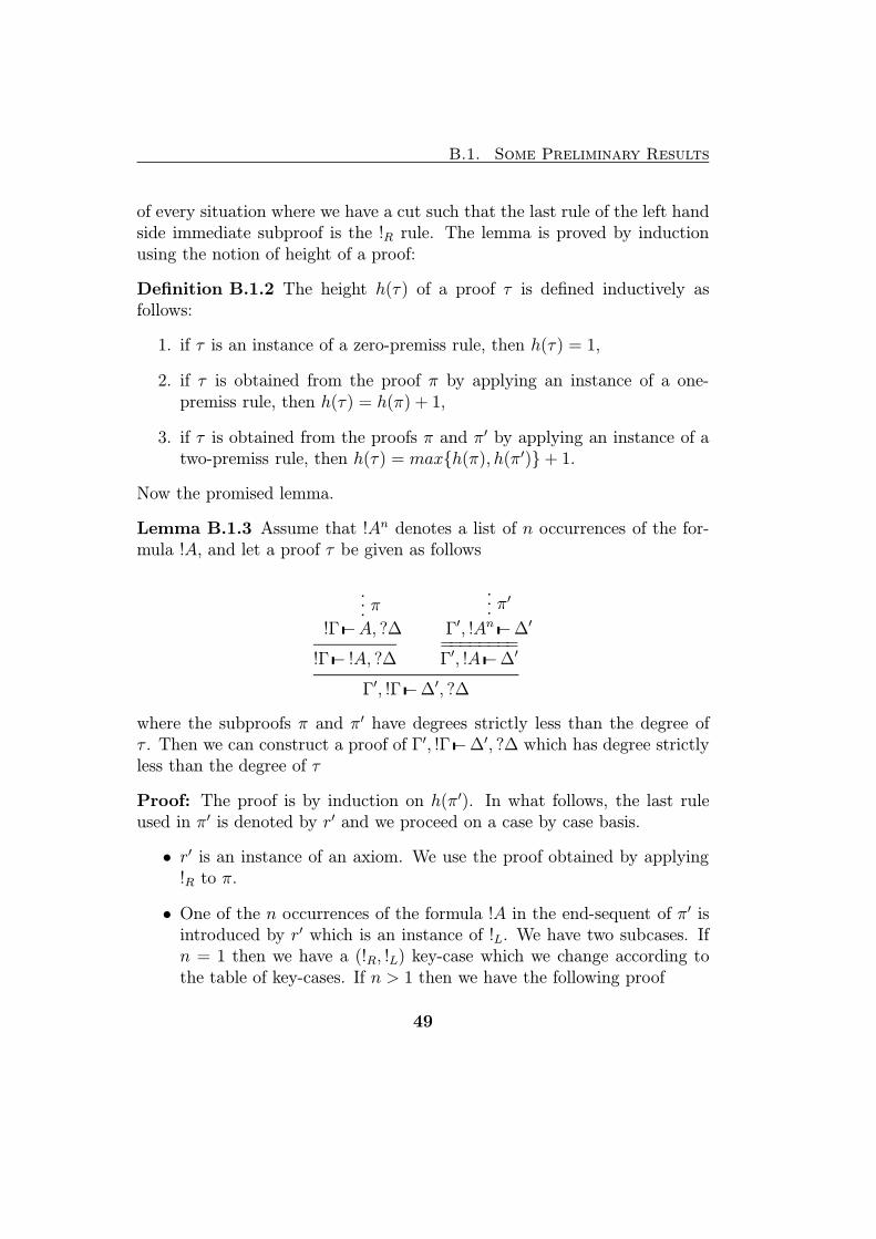
of every situation where we have a cut such that the last rule of the left handside immediate subproof is the !R rule. The lemma is proved by inductionusing the notion of height of a proof:

Definition B.1.2 The height h(τ) of a proof τ is defined inductively asfollows:

1. if τ is an instance of a zero-premiss rule, then h(τ) = 1,

2. if τ is obtained from the proof π by applying an instance of a one-premiss rule, then h(τ) = h(π) + 1,

3. if τ is obtained from the proofs π and π′ by applying an instance of atwo-premiss rule, then h(τ) = max{h(π), h(π′)}+ 1.

Now the promised lemma.

Lemma B.1.3 Assume that !An denotes a list of n occurrences of the for-mula !A, and let a proof τ be given as follows

··· π!Γ−A, ?∆

!Γ− !A, ?∆

··· π′

Γ′, !An−∆′

========Γ′, !A−∆′

Γ′, !Γ−∆′, ?∆

where the subproofs π and π′ have degrees strictly less than the degree ofτ . Then we can construct a proof of Γ′, !Γ−∆′, ?∆ which has degree strictlyless than the degree of τ

Proof: The proof is by induction on h(π′). In what follows, the last ruleused in π′ is denoted by r′ and we proceed on a case by case basis.

• r′ is an instance of an axiom. We use the proof obtained by applying!R to π.

• One of the n occurrences of the formula !A in the end-sequent of π′ isintroduced by r′ which is an instance of !L. We have two subcases. Ifn = 1 then we have a (!R, !L) key-case which we change according tothe table of key-cases. If n > 1 then we have the following proof

49


!Γ−A, ?∆

!Γ− !A, ?∆

Γ′, !An−1, A−∆′

Γ′, !An−1, !A−∆′

=============Γ′, !A−∆′

Γ′, !Γ−∆′, ?∆

which we transform into

!Γ−A, ?∆

!Γ−A, ?∆

!Γ− !A, ?∆

Γ′, !An−1, A−∆′

=============Γ′, !A,A−∆′

Γ′, !Γ, A−∆′, ?∆

Γ′, !Γ, !Γ−∆′, ?∆, ?∆=================

Γ′, !Γ−∆′, ?∆

on which we apply the induction hypothesis on the appropriate sub-proof.

• One of the n occurrences of the formula !A in the end-sequent of π′ isintroduced by r′ which is an instance of WL. We have two subcases. Ifn = 1 then we have a (!R,WL) key-case which we change according tothe table of key-cases. If n > 1 then we have the following proof

!Γ−A, ?∆

!Γ− !A, ?∆

Γ′, !An−1−∆′

Γ′, !An−1, !A−∆′

=============Γ′, !A−∆′

Γ′, !Γ−∆′, ?∆


!Γ−A, ?∆

!Γ− !A, ?∆

Γ′, !An−1−∆′

===========Γ′, !A−∆′

Γ′, !Γ−∆′, ?∆

on which we apply the induction hypothesis.

50


• One of the n occurrences of the formula !A in the end-sequent of π′

is introduced by r′ which is an instance of CL. We apply the induc-tion hypothesis to the immediate subproof of π′ where we consider theappropriate n+ 1 occurrences of !A.

• None of the n occurrences of the formula !A in the end-sequent of π′ areintroduced by r′. We have two subcases. In the first subcase all of then occurrences of the formula !A in the end-sequent of π′ are inheritedfrom the same immediate subproof. If r′ is a one-premiss rule, we havethe following proof

!Γ−A, ?∆

!Γ− !A, ?∆

Γ1, !An−∆1

r′

Γ′, !An−∆′

=========Γ′, !A−∆′

Γ′, !Γ−∆′, ?∆


!Γ−A, ?∆

!Γ− !A, ?∆

Γ1, !An−∆1

==========Γ1, !A−∆1

Γ1, !Γ−∆1, ?∆r′

Γ′, !Γ−∆′, ?∆

on which we apply the induction hypothesis on the appropriate sub-proof. The situation is analogous if r′ is a two-premiss rule. In thesecond subcase the n occurrences of the formula !A in the end-sequentof π′ are not inherited from the same immediate subproof, so we havethe following proof

!Γ−A, ?∆

!Γ− !A, ?∆

Γ1, !Ap−∆1 Γ2, !A

q −∆2r′

Γ′, !Ap+q −∆′

===========Γ′, !A−∆′

Γ′, !Γ−∆′, ?∆


51


!Γ−A, ?∆

!Γ− !A, ?∆

Γ1, !Ap−∆1

==========Γ1, !A−∆1

Γ1, !Γ−∆1, ?∆

!Γ−A, ?∆

!Γ− !A, ?∆

Γ2, !Aq −∆2

=========Γ2, !A−∆2

Γ2, !Γ−∆2, ?∆r′

Γ′, !Γ, !Γ−∆′, ?∆, ?∆=================

Γ′, !Γ−∆′, ?∆

on which we use the induction hypothesis on the appropriate two sub-proofs.

2

There is a dual to Lemma B.1.3; and it is the case that the proofs are alsodual.

B.2 Putting the Proof Together

The following lemma is the engine of the cut-elimination proof.

Lemma B.2.1 Let a proof τ be given as follows

··· πΓ−A,∆

··· π′

Γ′, A−∆′

Γ′,Γ−∆′,∆

where the subproofs π and π′ have degrees strictly less than the degree of τ .Then we can construct a proof of Γ′,Γ−∆′,∆ which has a degree strictlyless than the degree of τ .

Proof: Induction on h(π) + h(π′). In what follows, the last rules in π andπ′ are denoted by r and r′, respectively, and the immediate subproofs of πand π′ are denoted by πi and π′j , respectively. The formula A is denoted theprincipal formula. We proceed case by case.

• r is an instance of an axiom; we use π′.

• r′ is an instance of an axiom; dual to the previous case.

52

B.2. Putting the Proof Together

We have now dealt with the cases where r or r′ is an instance of an axiom.

• r is an instance of !R that introduces the principal formula; thus, A =!A′

for some A′, and π looks as follows:

!Γ−A′, ?∆

!Γ− !A′, ?∆

We use Lemma B.1.3.

• r′ is an instance of ?L that introduces the principal formula; dual tothe previous case.

• r is an instance of !R that does not introduce the principal formula;thus, A =?A′ for some A′, and π looks as follows:

!Γ−B, ?A′, ?∆

!Γ− !B, ?A′, ?∆

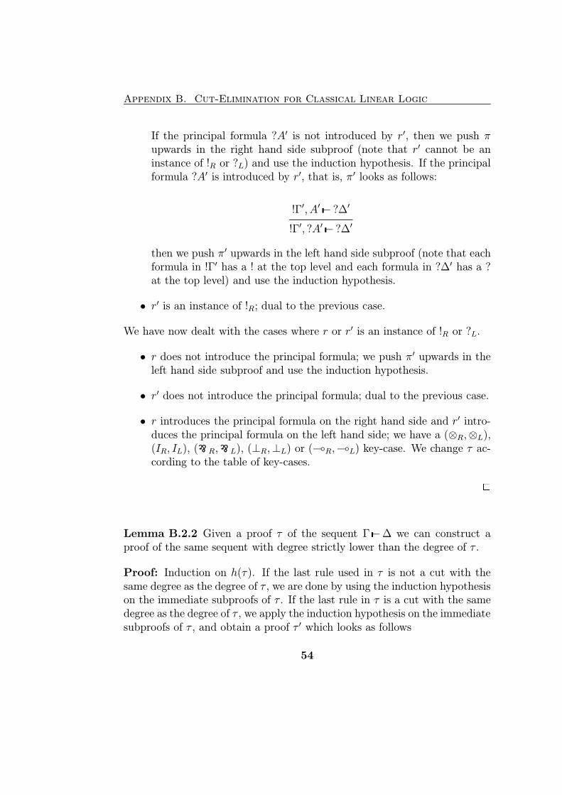
If the principal formula ?A′ is not introduced by r′, then we push πupwards in the right hand side subproof (note that r′ cannot be aninstance of !R or ?L) and use the induction hypothesis. If the principalformula ?A′ is introduced by r′, that is, π′ looks as follows:

!Γ′, A′− ?∆′

!Γ′, ?A′− ?∆′

then we push π′ upwards in the left hand side subproof (note that eachformula in !Γ′ has a ! at the top level and each formula in ?∆′ has a ?at the top level) and use the induction hypothesis.

• r′ is an instance of ?L that does not introduce the principal formula;dual to the previous case.

• r is an instance of ?L; thus, A =?A′ for some A′, and π looks as follows:

!Γ, B− ?A′, ?∆

!Γ, ?B− ?A′, ?∆

53


If the principal formula ?A′ is not introduced by r′, then we push πupwards in the right hand side subproof (note that r′ cannot be aninstance of !R or ?L) and use the induction hypothesis. If the principalformula ?A′ is introduced by r′, that is, π′ looks as follows:

!Γ′, A′− ?∆′

!Γ′, ?A′− ?∆′

then we push π′ upwards in the left hand side subproof (note that eachformula in !Γ′ has a ! at the top level and each formula in ?∆′ has a ?at the top level) and use the induction hypothesis.

• r′ is an instance of !R; dual to the previous case.

We have now dealt with the cases where r or r′ is an instance of !R or ?L.

• r does not introduce the principal formula; we push π′ upwards in theleft hand side subproof and use the induction hypothesis.

• r′ does not introduce the principal formula; dual to the previous case.

• r introduces the principal formula on the right hand side and r′ intro-duces the principal formula on the left hand side; we have a (⊗R,⊗L),(IR, IL), (..................................................

.............................................R,

...............................................................................................L), (⊥R,⊥L) or ((R,(L) key-case. We change τ ac-

cording to the table of key-cases.

2

Lemma B.2.2 Given a proof τ of the sequent Γ−∆ we can construct aproof of the same sequent with degree strictly lower than the degree of τ .

Proof: Induction on h(τ). If the last rule used in τ is not a cut with thesame degree as the degree of τ , we are done by using the induction hypothesison the immediate subproofs of τ . If the last rule in τ is a cut with the samedegree as the degree of τ , we apply the induction hypothesis on the immediatesubproofs of τ , and obtain a proof τ ′ which looks as follows

54

B.2. Putting the Proof Together

··· πΓ′−A,∆′

··· π′

Γ′′, A−∆′′

Γ′′,Γ′−∆′′,∆′

where the proofs π and π′ have degrees strictly lower than the degree ofτ ′. Note that Γ′′,Γ′ is equal to Γ and ∆′′,∆′ is equal to ∆. We then useLemma B.2.1. 2

And now the Hauptsatz.

Theorem B.2.3 Given any proof of a sequent we can construct a cut-freeproof of the same sequent.

Proof: Iteration of Lemma B.2.2. 2

55

Recent Publications in the BRICS Lecture Series

LS-96-6 Torben Brauner. Introduction to Linear Logic. December1996. iiiv+55 pp.

LS-96-5 Devdatt P. Dubhashi. What Can’t You Do With LP? De-cember 1996. viii+23 pp.

LS-96-4 Sven Skyum. A Non-Linear Lower Bound for MonotoneCircuit Size. December 1996. viii+14 pp.

LS-96-3 Kristoffer H. Rose. Explicit Substitution – Tutorial & Sur-vey. September 1996. v+150 pp.

LS-96-2 Susanne Albers.Competitive Online Algorithms. Septem-ber 1996. iix+57 pp.

LS-96-1 Lars Arge. External-Memory Algorithms with Applica-tions in Geographic Information Systems. September 1996.iix+53 pp.

LS-95-5 Devdatt P. Dubhashi. Complexity of Logical Theories.September 1995. x+46 pp.

LS-95-4 Dany Breslauer and Devdatt P. Dubhashi.Combinatoricsfor Computer Scientists. August 1995. viii+184 pp.

LS-95-3 Michael I. Schwartzbach. Polymorphic Type Inference.June 1995. viii+24 pp.

LS-95-2 Sven Skyum. Introduction to Parallel Algorithms. June1995. viii+17 pp. Second Edition.

LS-95-1 Jaap van Oosten.Basic Category Theory. January 1995.vi+75 pp.

introduction to linear logic - brics · formulation of classical logic can be obtained by leaving...

Documents