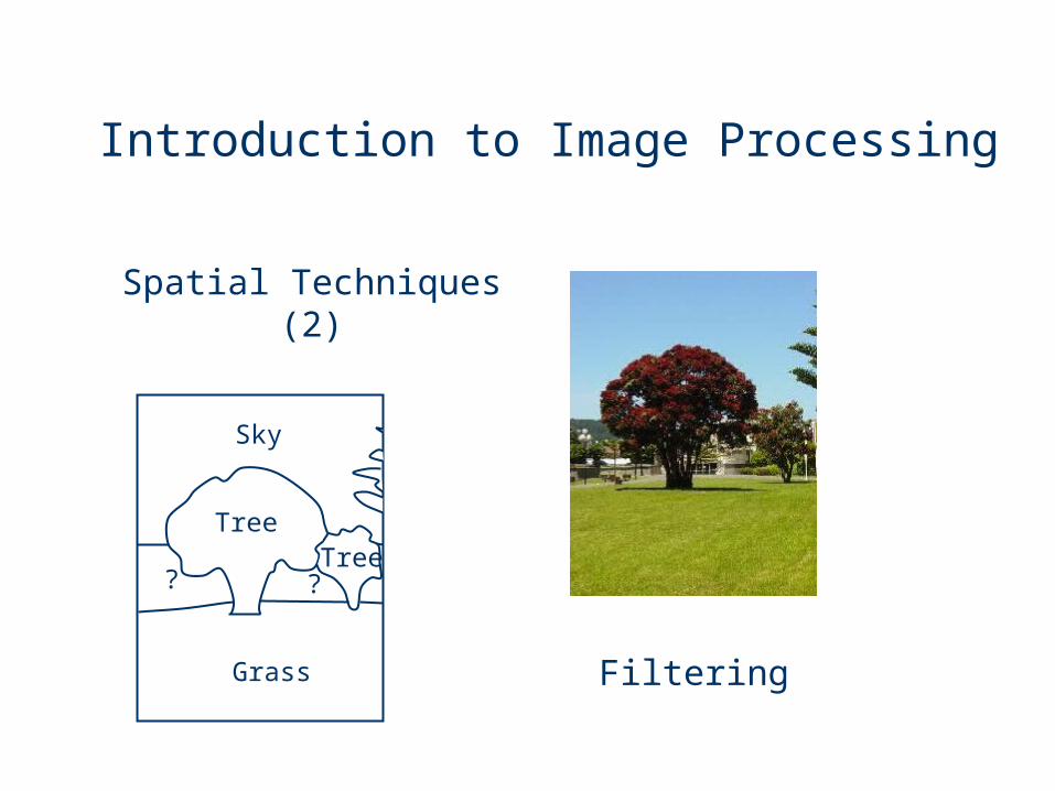
Introduction to Image Processing

Grass

Sky

TreeTree

? ?

Spatial Techniques (2)

Filtering

Spatial Techniques

• Neighbourhood Operations• Linear System Theory

– Unit Pulse Response• Convolution & Correlation• Image Filtering

‒ Linear − Non-linear

Neighbourhood Operations

• Operation at a pixel depends on the grey level values of a region of interest surrounding that pixel

• Neighbourhood is assumed to be centred at a pixel, thus normally it is a square with odd dimensions

• For point operations, the original input pixel value is no more needed once it has been processed. Neighbourhood operators, however, need the original pixel value for subsequent calculations of other neighbourhoods that also include that specific pixel

• applications include blurring, sharpening, noise reduction, edge detection, feature identification, measuring the similarity of two images

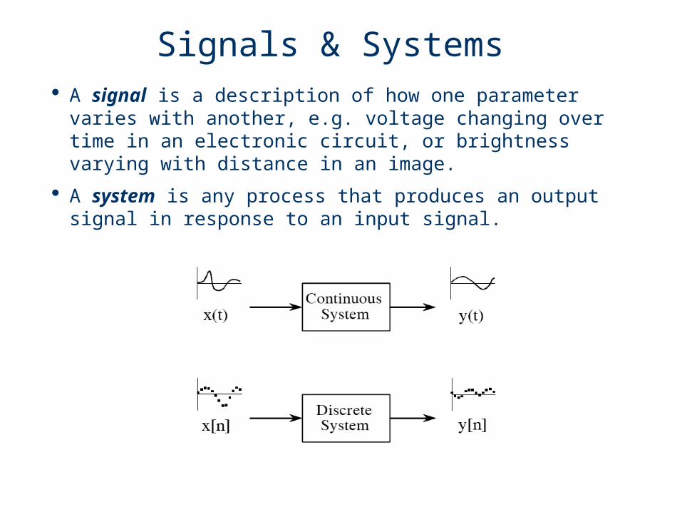
· A signal is a description of how one parameter varies with another, e.g. voltage changing over time in an electronic circuit, or brightness varying with distance in an image.

· A system is any process that produces an output signal in response to an input signal.

Signals & Systems

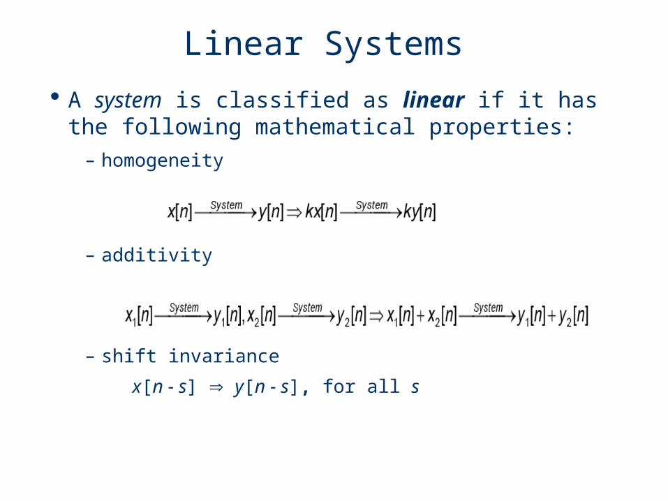
· A system is classified as linear if it has the following mathematical properties:

– homogeneity

– additivity

– shift invariance

x[n - s] y[n - s], for all s

Linear Systems

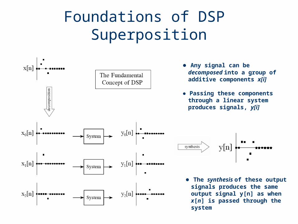
● Any signal can be decomposed into a group of additive components x[i]

● Passing these components through a linear system produces signals, y[i]

● The synthesis of these output signals produces the same output signal y[n] as when x[n] is passed through the system

Foundations of DSP Superposition

Characterising Linear Systems

· Any linear digital image processing system can be characterised by one of two following equivalent ways:

– unit pulse (impulse) response

– frequency response

· Unit pulse (impulse) response

– when the unit pulse is passed through a linear system, the single non-zero point will be changed into some other 2-D pattern

– since the only thing that can happen to a point is that it spreads out, it is often called the point spread function (PSF) in image processing jargon

– it is an effective way to model an imaging system, as any image can be viewed as a sum of scaled and shifted unit pulses

Convolution and Correlation

· Many image processing operations can be modeled as a linear system.

· Convolution and correlation are the two fundamental neighbourhood operations of image processing

· Convolution takes two signals and produces a third signal as output. Its main application is the filtering of images, e.g. sharpening the edges of objects, reducing random noise, correcting unequal illumination, blur and motion.

· Correlation measures similarity of two images which is useful in feature recognition and in registration, where we wish to place one image relative to another at a position of maximum similarity.

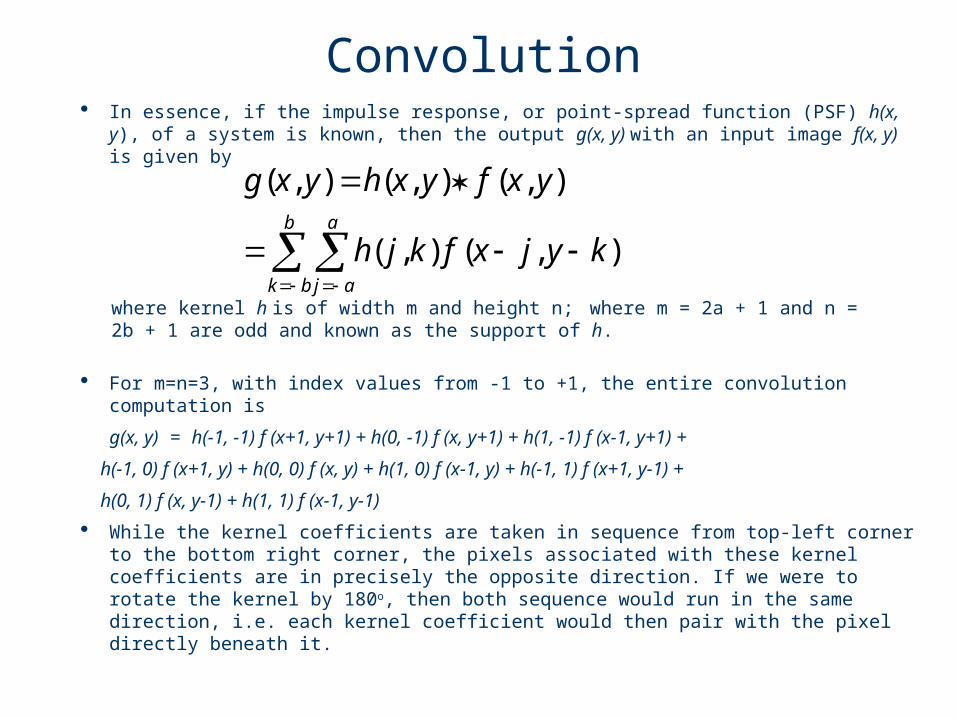
Convolution· In essence, if the impulse response, or point-spread function (PSF) h(x, y), of a

system is known, then the output g(x, y) with an input image f(x, y) is given by

b

bk

a

aj

kyjxfkjh

yxfyxhyxg

),(),(

),(),(),(

where kernel h is of width m and height n; where m = 2a + 1 and n = 2b + 1 are odd and known as the support of h.

· For m=n=3, with index values from -1 to +1, the entire convolution computation is

g(x, y) = h(-1, -1) f (x+1, y+1) + h(0, -1) f (x, y+1) + h(1, -1) f (x-1, y+1) +

h(-1, 0) f (x+1, y) + h(0, 0) f (x, y) + h(1, 0) f (x-1, y) + h(-1, 1) f (x+1, y-1) +

h(0, 1) f (x, y-1) + h(1, 1) f (x-1, y-1)

· While the kernel coefficients are taken in sequence from top-left corner to the bottom right corner, the pixels associated with these kernel coefficients are in precisely the opposite direction. If we were to rotate the kernel by 180o, then both sequence would run in the same direction, i.e. each kernel coefficient would then pair with the pixel directly beneath it.

· Using the same notation of convolution, if the template is represented as h(x, y), the output g(x, y) with an input image f (x, y) is given by

where template h is of width m and height n and m = 2a + 1, n = 2b + 1.

• Mathematically, convolution is the same process, except that h is rotated by 180 degree.

• When h(x, y) is symmetric, convolution is equal to correlation.

Correlation

b

bk

a

aj

kyjxfkjh

yxfyxhyxg

),(),(

),(),(),(

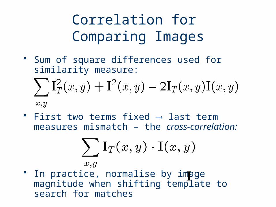
Correlation for Comparing Images

• Sum of square differences used for similarity measure:

• First two terms fixed last term measures mismatch – the cross-correlation:

• In practice, normalise by image magnitude when shifting template to search for matches

Template Matching

• The filter is called a template or a mask

• The brighter the value in the output, the better the match

Input image

Template

Output

Removing Noise (Denoising)Spatial Domain

• Some sorts of processing are sensitive to noise• We want to remove the effects of noise before

going further• However, we may lose information in doing so

• Most noise removal processes are called filtering

• They are applied to each point in an image through convolution

• They use information in a small local window of pixels

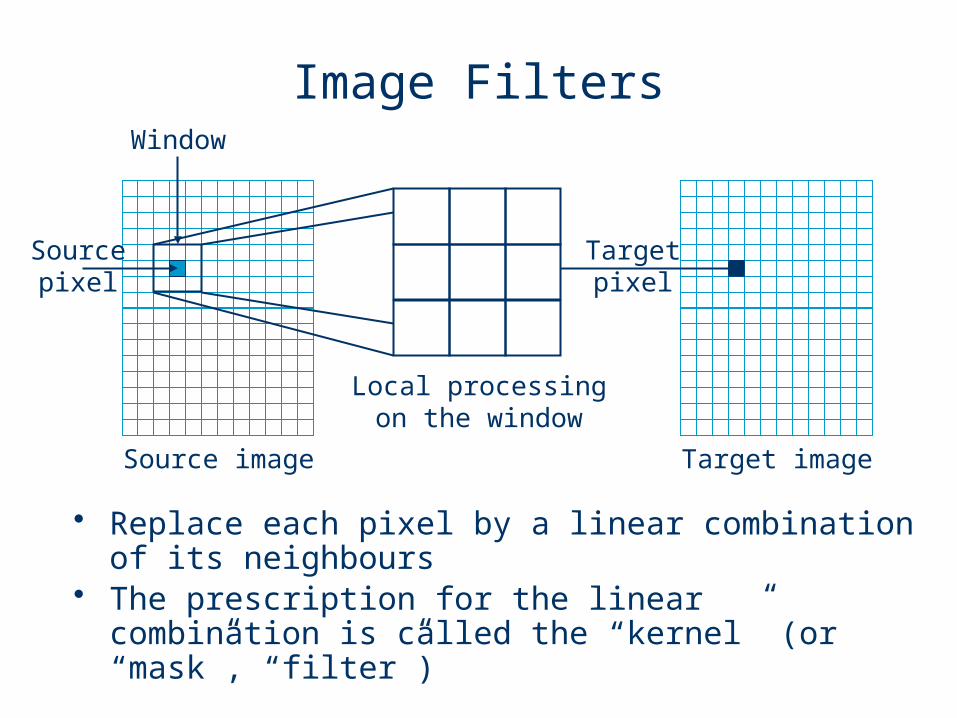
Image Filters

Source image Target image

Sourcepixel

Window

Local processingon the window

Targetpixel

• Replace each pixel by a linear combination of its neighbours

• The prescription for the linear combination is called the “kernel” (or “mask”, “filter”)

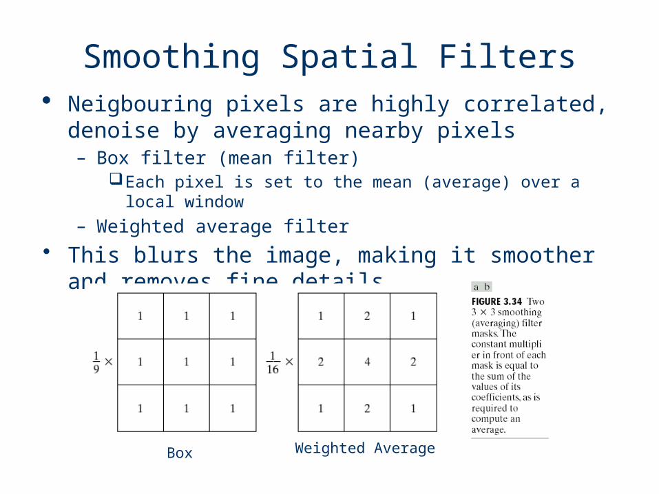
· Neigbouring pixels are highly correlated, denoise by averaging nearby pixels– Box filter (mean filter)

Each pixel is set to the mean (average) over a local window

– Weighted average filter• This blurs the image, making it smoother and

removes fine details

Box Weighted Average

Smoothing Spatial Filters

4.3

Step 1: Move the window to the first location where we want to compute the average value and then select only pixels inside the window.

4

4

67

6

1

9

2

2

2

7

5

2

26

4

4

5

212

1

3

3

4

2

9

5

7

7

Step 2: Computethe average value

3

1

3

1

),(9

1

i j

jipy

Sub image p

Original image

4 1

9

2

2

3

2

9

7

Output image

Step 3: Place theresult at the pixelin the output image

Step 4: Move the window to the next location and go to Step 2

Basics of Spatial Filtering

Gaussian Filter

• Gaussian filters are based on the same function used for Gaussian noise

• To generate a filter it needs to be 2D− If we take the mean to be 0 then we get

2

2

2σ

μ)(x

e2πσ

1P(x)

2

22

2σ

)y(x

2e

2πσ

1y)P(x,

Gaussian Filter

• The Gaussian filter has a 2D bell shape− It is symmetric around the centre− The centre value gets the highest weight− Values further from the centre get lower weights

2-D Gaussian distribution with mean (0,0) and standard deviation 1

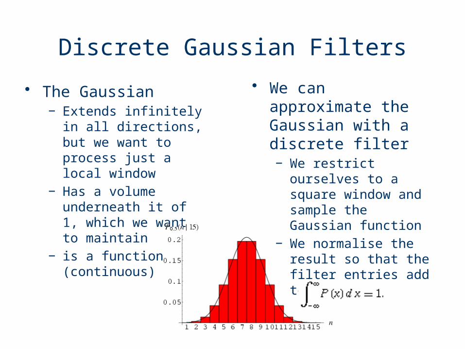
Discrete Gaussian Filters

• The Gaussian− Extends infinitely in

all directions, but we want to process just a local window

− Has a volume underneath it of 1, which we want to maintain

− is a function (continuous)

• We can approximate the Gaussian with a discrete filter− We restrict ourselves

to a square window and sample the Gaussian function

− We normalise the result so that the filter entries add to 1

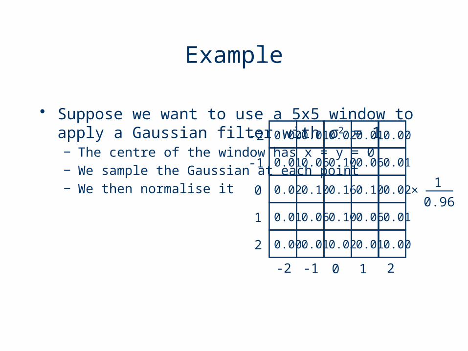
Example

• Suppose we want to use a 5x5 window to apply a Gaussian filter with σ2 = 1− The centre of the window has x = y = 0− We sample the Gaussian at each point− We then normalise it

0 1 2-1-2

0

1

2

-1

-2 0.00 0.01 0.02 0.01 0.00

0.01 0.06 0.10 0.06 0.01

0.02 0.10 0.16 0.10 0.02

0.01 0.06 0.10 0.06 0.01

0.00 0.01 0.02 0.01 0.00

×1

0.96

Averaging vs. Gaussian Filters• Advantages of Gaussian filtering

− rotationally symmetric (isotropic)− filter weights decrease monotonically from central

peak, giving most weight to central pixels− separable

Separable Filters

• The Gaussian filter is separable− This means you can do a 2D Gaussian as 2 1D

Gaussians− First you filter with a ‘horizontal’ Gaussian− Then with a ‘vertical’ Gaussian

P(y)P(x)

e2πσ

1e

2πσ

1

ee2πσ

1

2πσ

1

e2πσ

1y)P(x,

2

2

2

2

2

2

2

2

2

22

2σ

y

2σ

x

2σ

y

2σ

x

2σ

)y(x

2

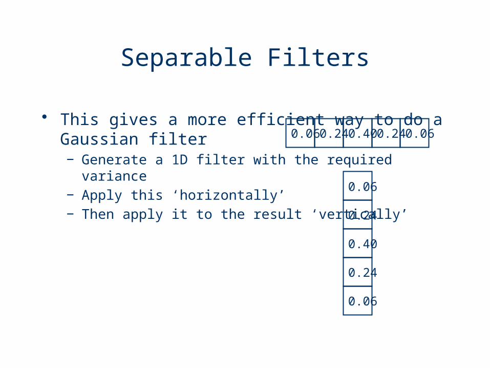
Separable Filters

• This gives a more efficient way to do a Gaussian filter− Generate a 1D filter with the required variance− Apply this ‘horizontally’− Then apply it to the result ‘vertically’

0.06 0.24 0.40 0.24 0.06

0.06

0.24

0.40

0.24

0.06

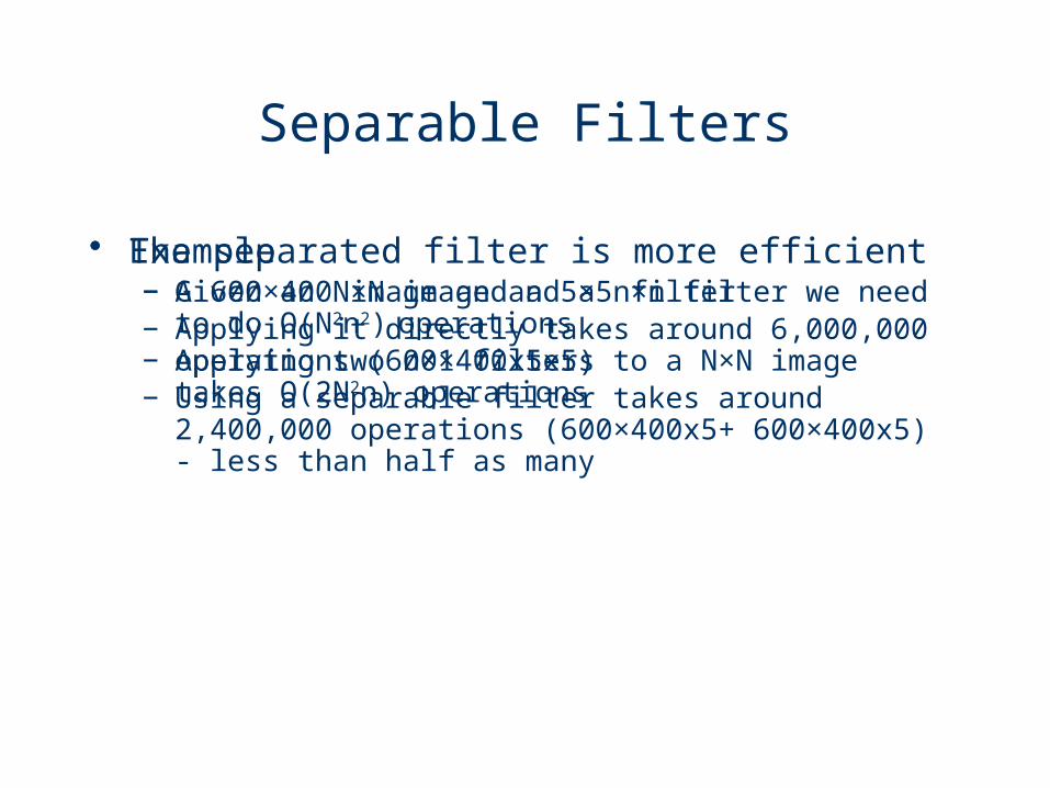
Separable Filters

• The separated filter is more efficient− Given an N×N image and a n×n filter we need to do

O(N2n2) operations− Applying two n×1 filters to a N×N image takes

O(2N2n) operations

• Example− A 600×400 image and a 5×5 filter− Applying it directly takes around 6,000,000

operations (600×400x5x5)− Using a separable filter takes around 2,400,000

operations (600×400x5+ 600×400x5) - less than half as many

Gaussian Filters

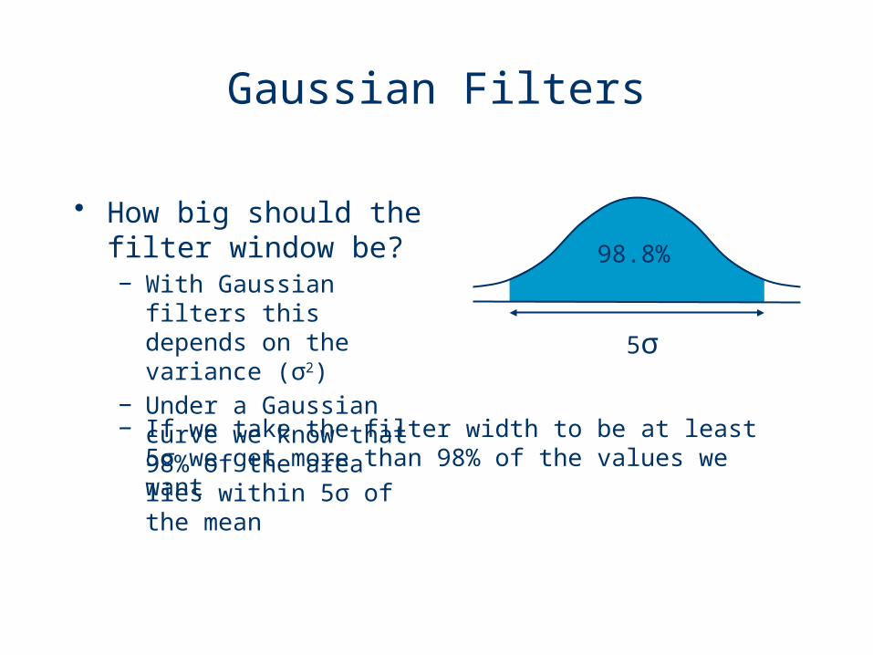
• How big should the filter window be?− With Gaussian filters

this depends on the variance (σ2)

− Under a Gaussian curve we know that 98% of the area lies within 5σ of the mean

− If we take the filter width to be at least 5σ we get more than 98% of the values we want

5σ

98.8%

Spatial Non-Linear FilteringAs in the case of linear filtering, we consider a subimage Sxy centred at a certain pixel (x,y) of the image. The new value of the image at the pixel (x,y) is a non-linear function of the values of Sxy, such as:

Original image Processed image

Centre

Min

Max

Median

)},({min),(ˆ),(

tsfyxfxySts

)},({max),(ˆ),(

tsfyxfxySts

)},({median),(ˆ),(

tsfyxfxySts

Example

Image with salt

noise

Image denoised with a 3x3 min

filter

Example

Image with

pepper noise

Image denoised with a 3x3 max

filter

Nonlinear Median Filter

• An alternative to the mean filter is the median filter− Statistically the median is the middle value in a set− Each pixel is set to the median value in a local

window

123124125

129127 9

126123131

123124125129127 9 126123131

Find the values in a local window

9 123123124125126127129131

Sort them9 123123124125126127129131

Pick the middle one

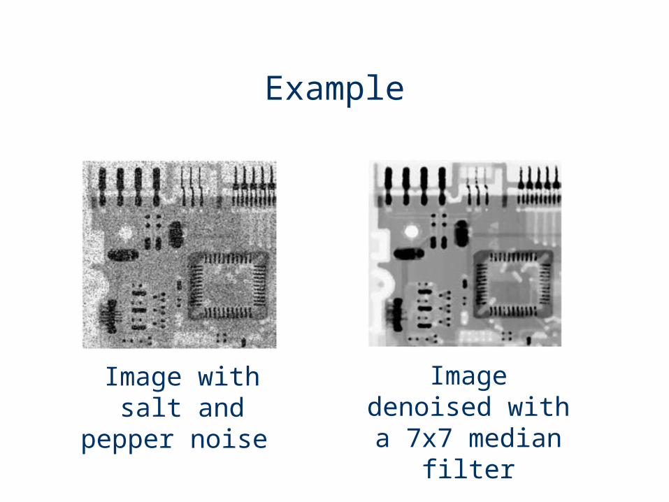
Example

Image with salt and pepper

noise

Image denoised with a 7x7

median filter

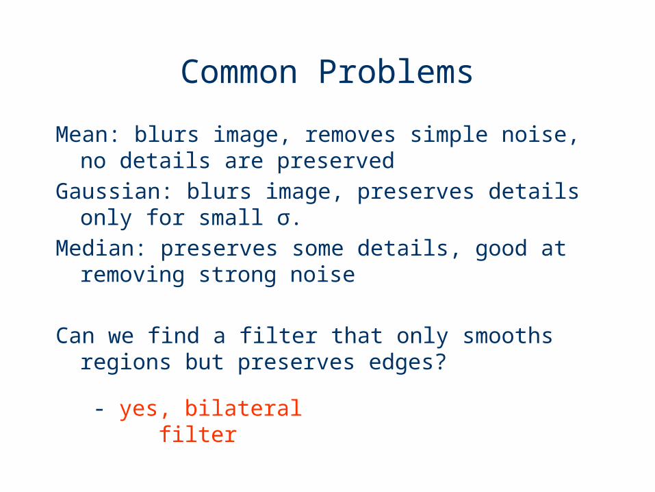
Common Problems

Mean: blurs image, removes simple noise, no details are preserved

Gaussian: blurs image, preserves details only for small σ.

Median: preserves some details, good at removing strong noise

Can we find a filter that only smooths regions but preserves edges?

- yes, bilateral filter

Illustration a 1D Image

• 1D image = line of pixels

• Better visualized as a plot

pixelintensity

pixel position

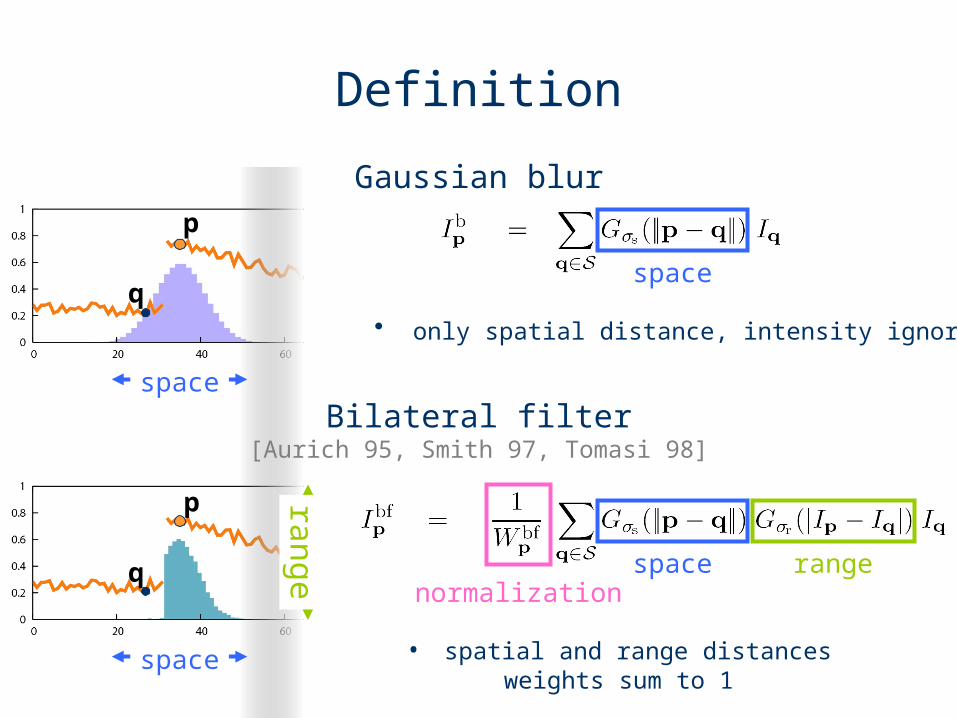
Definition

space rangenormalization

space

Gaussian blur

Bilateral filter[Aurich 95, Smith 97, Tomasi 98]

• only spatial distance, intensity ignored

• spatial and range distancesweights sum to 1

space

spacerange

p

p

q

q

Gaussian Smoothing

*

*

*

input output

Same Gaussian kernel everywhereAverages across edges blur

Slides taken from Sylvain Paris, Siggraph 2007

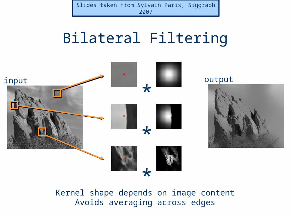
Bilateral Filtering

*

*

*

input output

Kernel shape depends on image contentAvoids averaging across edges

Slides taken from Sylvain Paris, Siggraph 2007

The Problem with Edges

• We have seen two ways to filter images− Mean filter - take the average value over a local window− Median filter - take the middle value over a local window

• Filters operate on a local window− We need to know the value of all the neighbours of each pixel− Pixels on the edges or corners of the image don’t have all their

neighbours

? ??

?

?

Dealing with Edges

• There are a number of ways we can deal with edges− Ignore them - don’t use filters near edges− Modify our filter to account for smaller

neighbourhoods− Extend the image to predict the unknowns

• Ignoring the edges− This is simple − It means that we lose the border pixels each time we

apply a filter− Might be OK for one or two small filters, but your

image can shrink rapidly

Modifying the Filter

• Many filters can be modified to give a reasonable value near the edge− We may need different filters for top, bottom, left,

and right edges, and for each corner

• Example: mean filter

1/61/61/6

1/61/61/6

1/61/61/6

1/61/61/6

1/61/6

1/6

1/61/6

1/6

1/61/6

1/6

1/61/6

1/6

1/41/4

1/41/4

1/41/4

1/41/4

1/41/4

1/41/4

1/41/4

1/41/4

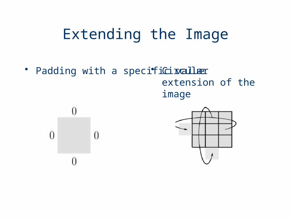
Extending the Image

• Padding with a specific value• Circular extension of the image

Extending the Image

• We need to predict what lies beyond the edges of the image− We can use the value

of the nearest known pixel

− We can apply a more detailed model to the image

• Nearest neighbour

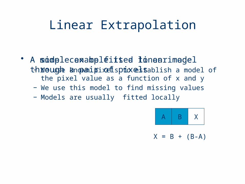
Linear Extrapolation

• A model can be fitted to an image− We use known pixels to establish a model of the pixel

value as a function of x and y− We use this model to find missing values− Models are usually fitted locally

• A simple example is a linear model through a pair of pixels

A B X

X = B + (B-A)

Linear Extrapolation

130 133

136 138

130 + (130-133)

136 + (136-138)

127

134

136 + (136-133)

139

136 + (136-130)

142

138 + (138-133)

143

Code for filters

• With a filter the processing at (x,y) depends on a neighbourhood, typically a square with ‘radius’ r (3x3 has radius 1, 5x5 radius 2…)

int x, y, dx, dy, r;for (x = 0; x < image.getWidth(); x++) { for (y = 0; y < image.getHeight(); y++) { for (dx = -r; dx <= r; dx++) { for (dy = -r; dy <= r; dy++) {

// Do something with (x+dx, y+dy)}}}}

For eachpixel, p

For each pixel in theneighbourhood of p

• function gaussianfilter()• • % Parameters of the Gaussian filter:• n1=10;sigma1=3;n2=10;sigma2=3;theta

=0;• % The amplitude of the noise:• noise=10;• • [w,map]=imread('lena.gif', 'gif'); • x=ind2gray(w,map);• x_rand=noise*randn(size(x));• [m,n]=size(x);• • for i=1:m• for j=1:n • y(i,j)=x(i,j)+x_rand(i,j);• j=j+1;• end• i=i+1;• end • • filter1=d2gauss(n1,sigma1,n2,sigma2,thet

a);• • f1=conv2(x,filter1,'same');• f2=conv2(y,filter1,'same');• • figure(1);• subplot(2,2,1);imagesc(x);title('lena');• subplot(2,2,2);imagesc(y);title('noisy');• subplot(2,2,3);imagesc(f1);title('Gaussian

filter lena - smooth');• subplot(2,2,4);imagesc(f2);title('Gaussian

filter noisy - noise removal');• colormap(gray);• return;

• % Function "d2gauss.m":

• % This function returns a 2D Gaussian filter with size n1*n2; theta is

• % the angle that the filter rotated counter clockwise; and sigma1 and sigma2

• % are the standard deviation of the Gaussian functions.

• • function h = d2gauss(n1,std1,n2,std2,theta)• r=[cos(theta) -sin(theta);• sin(theta) cos(theta)];• for i = 1 : n2 • for j = 1 : n1• u = r * [j-(n1+1)/2 i-(n2+1)/2]';• h(i,j)=gauss(u(1),std1)*gauss(u(2),std2);• end• end• h = h / sqrt(sum(sum(h.*h)));• • % Function "gauss.m":• function y = gauss(x,std)• y = exp(-x^2/(2*std^2)) / (std*sqrt(2*pi));

• http://en.wikipedia.org/wiki/Gaussian_function

Acknowlegements

Slides are modified based on the original slide set from Dr Li Bai, The University of Nottingham, Jubilee Campus plus the following sources:

• Digital Image Processing, by Gonzalez and Woods• Digital Image Processing: a practical introduction using

Java, by Nick Efford• http://gear.kku.ac.th/~nawapak/178353/Chapter03.ppt • http://www.comp.dit.ie/bmacnamee/materials/dip/lectures/

ImageProcessing5-SpatialFiltering1.ppt• The Scientist and Engineer’s Guide to Digital Signal

Processing, by Steven W. Smith