Introduction to Image Processing

Grass

Sky

TreeTree

? ?

Image Segmentation

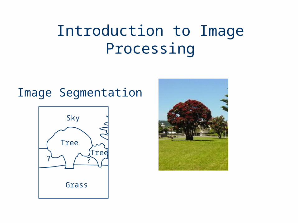
• Image segmentation is the partitioning of an image into non-overlapping, constituent regions that are homogeneous with respect to some characteristics.

• If one views an image as depicting a scene composed of different objects, regions, etc. then segmentation is the decomposition of an image into these objects and regions by associating or “labelling” each pixel with the object that it corresponds to.

• It is an essential step for image analysis, object representation, visualisation and many other image processing tasks.

Image Segmentation

Image Segmentation

• Most humans can segment an image with ease.

• Computer automated segmentation is a difficult problem, requiring sophisticated algorithms to work in tandem.

• High level segmentation, such as segmenting humans, cars etc., from an image is a very difficult problem. It is considered an unsolved problem and is still under active research.

Image Segmentation

Perfect image segmentation is usually difficult to achieve due to the following:– a pixel may straddle the “real” boundary of objects

such that it partially belong to two or more objects– effects of noise, non-uniform illumination, occlusions

etc. that give rise to the problem of over-segmentation and under-segmentation

In over-segmentation, pixels belonging to the same object are classified as belonging to different segments while in under-segmentation, pixels belonging to different objects are classified as belonging to the same object

Image Segmentation

For the most part there are fundamentally two kinds of approaches to segmentation: discontinuity and similarity. – similarity may be due to pixel intensity, colour

or texture. – differences are sudden changes

(discontinuities) in any of these, but especially sudden changes in intensity across a boundary, which is called an edge.

Finding Objects in Images

• To do this we need to divide the image into two parts– the object of interest

(the foreground)– everything else (the

background)

• The definition of foreground and background depends on the task at hand

Grass

Sky

TreeTree

? ?

A Simple Method - Thresholding

• If the image contains a dark object on a light background– choose a threshold

value, T– for each pixel

if the brightness at that pixel is less than T it is on the object

otherwise it is part of the background

Threshold, T = 96

Choosing a Threshold

• The value of the threshold is very important– if it is too high then

background pixels will be classified as foreground

– if it is too low then foreground pixels will be classified as background

T = 128

T = 64

Image Histograms

• To find a threshold we can use an image histogram– count how many pixels

in the image have each value

– shows peaks around regions of the image

• The seal image shows three regions– one below T1 = 80– one above T2 = 142– one between the two

thresholds

Basic Global ThresholdingIterative Algorithm

• Select an initial estimate for the global threshold, T. The average intensity of the image is a good initial choice for T.

• Segment the image using T. This will produce two groups of pixels: G1 consisting of all pixels with grey level values > T and G2 consisting of pixels with grey level values T

• Compute the average (mean) intensity values 1 and 2 for the pixels in regions G1 and G2 respectively.

• Compute a new threshold value: T = 0.5 (1 + 2)

• Repeat steps 2 through 4 until the difference between values of T in successive iterations is smaller than a predefined parameter To.

Connected Components

• The seal is now a large black blob in the image, but– not all the black pixels

are on the seal– not all the pixels on the

seal are black

• We can deal with the first problem by finding connected components in the image

• The second problem is much harder

• Each object in the image is (hopefully)– all same colour– all in one piece– not merged with any other

objects with the same colour

• Finding connected component - given one pixel on the object– all of its neighbours with

the same colour are on the object

– their neighbours’ neighbours with the same colour are on the object

– and so on...

Connected Components

Input: A pixel p on the objectAlgorithm:Make two lists, object and searchAdd p to searchWhile (search is not empty) Remove a pixel q from searchAdd q to object

For each neighbour n of q If n is not in object AND I(n) = I(p)

Add it to search

p (x+1,y)(x-1,y)

(x,y-1)

(x,y+1)

4-neighbours of p:

N4(p)= (x1,y)(x+1,y)(x,y1)(x,y+1)

p (x+1,y)(x-1,y)

(x,y-1)

(x,y+1)

(x+1,y-1)(x-1,y-1)

(x-1,y+1) (x+1,y+1)

(x1,y1)(x,y1)

(x+1,y1)(x1,y)(x+1,y)

(x1,y+1)(x,y+1)

(x+1,y+1)

N8(p)=

8-neighbours of p:

Neighbours of a Pixel

Otsu’s Thresholding Method

• Based on a very simple idea: Find the threshold that minimises the weighted within-class variance

• This turns out to be the same as maximising the between-class variance

• Operates directly on the grey level histogram [e.g. 256 numbers, p(i)], so it’s fast (once the histogram is computed)

(1979)

The weighted within-class variance is:

)()()()()( 222

211

2 kkPkkPkw

where the class probabilities are estimated as:

k

i

ipkP0

1 )()(

1

12 )()(

L

ki

ipkP

k

i kP

iipkm

0 11 )(

)()(

1

1 22 )(

)()(

L

ki kP

iipkm

and the class means are given by:

Calculation of Within Class Variance

Finally, the individual class variances are:

k

i kP

ipkmik

1 1

21

21 )(

)()]([)(

L

ki kP

ipkmik

1 2

22

22 )(

)()]([)(

Now, we could actually stop here. All we need to do is just run through the full range of k values [0,255] and pick the value that minimises

But the relationship between the within-class and between-class variances can be exploited to allow a much faster calculation. (Refer to recommended text by Gonzalez on how between-class variance is used instead)

)(2 kw

Calculation of Within Class Variance

Basic Adaptive Thresholding

• Subdivide original image into small areas.

• Utilize a different threshold to segment each subimages.

• Since the threshold used for each pixel depends on the location of the pixel in terms of the subimages, this type of thresholding is adaptive.

Example : Adaptive Thresholding

Multilevel Thresholding

• A point (x,y) belongs to – to an object class if T1 < f(x,y) T2

– to another object class if f(x,y) > T2

– to background if f(x,y) T1

• Tn depends on – only f(x,y) : only on gray-level

values global threshold– both f(x,y) and p(x,y) : on gray-level

values and its neighbours Local threshold

• The algorithm of connected components can be applied iteratively to isolate and label each individual object

• Connected component labelling works by scanning an image, pixel-by-pixel (from top to bottom and left to right) in order to identify connected pixel regions, i.e. regions of adjacent pixels which share the same set of intensity values.

Identify Individual Object

• Scan the image by moving along a row until it comes to a point p (where p denotes the pixel to be labelled at any stage in the scanning process) for which V={1}. When this is true, it examines the four neighbours of p which have already been encountered in the scan (in the case of 8-connectivity, the neighbours (i) to the left of p, (ii) above it, and (iii and iv) the two upper diagonal terms). Based on this information, the labelling of p occurs as follows:

• If all four neighbours are 0, assign a new label to p, else• if only one neighbour has V={1}, assign its label to p, else• if more than one of the neighbours have V={1}, assign one of the

labels to p and make a note of the equivalences.

• After completing the scan, the equivalent label pairs are sorted into equivalence classes and a unique label is assigned to each class.

• As a final step, a second scan is made through the image, during which each label is replaced by the label assigned to its equivalence classes. For display, the labels might be different grey levels or colours.

Labelling Algorithm

• (8-connectivity)

1 1 1 1

1 1

1 1

1 1

1

1 1 1

1 1 2 2

1 1

1 1

3 1

3

3 3 3

Equivalent labels

{1, 2}

Original Binary Image After first scan

Labelling Algorithm - Example

• (8-connectivity)

1 1 2 2

1 1

1 1

3 1

3

3 3 3

Equivalent labels

{1, 2}

After 1st scan

1 1 1 1

1 1

1 1

2 1

2

2 2 2

Final label

1: {1, 2}2: {3}

After 2nd scan (two individual objects/regions have been identified)

Labelling Algorithm - Example

• Connected Component Labeling: Give pixels belonging to the same object the same label (grey level or colour)

Identify Individual Object

Another Method – Edge Based• Due to imperfections, the set of pixels given by

edge detection methods seldom characterises an edge completely. Spurious intensity discontinuities and breaks in the edge is usual. Thus linking procedure following edge detection to assemble edge pixels into meaningful edges are needed.

• Commonly used post-processing techniques are:– local processing– global processing via the Hough transform– other processing methods

Local Processing• Similarity-based methods: two principal properties used

for establishing similarity of edge pixels are: – the strength of the response of the gradient operator

used to produce the edge pixels;– the direction of gradient vector

where the edge point (x0, y0) locates in the predefined neighborhood of point (x, y). When both similarities are satisfied, the two point are linked.

0 0

0 0

( , ) ( , )

( , ) ( , )

f x y f x y E

x y x y A

Global ProcessingThe Hough Transform

• The Hough is a general technique for extracting geometrical primitives from e.g. edge data

• We will look at the basic method and how it can be used to find straight lines and circles

Why Find Lines, etc?

• Edge detectors mark interesting features of the world, but produce a binary image after thresholding operation

• By fitting lines, circles, ellipses, etc we group edge points together to give fewer, more significant entities

The Problem

• High level features such as lines are important

• Edge detection provides a set of points (xi, yi) which are likely to lie on those lines

• But how many lines are there and what are their parameters?

• The Hough Transform

y

x

Line Parameters

• The standard equation of a line is

y = mx +c

• This line represents the set of (x,y) pairs that satisfy the line equation

• If we know the line parameters m,c we can vary x, compute y and draw the line

y

x

y = mx + c

• But we don’t know the line parameters - we just have some data points (xi,yi)

Parameter Space

• If a data point (xi,yi) lies on a line then that line’s parameters m,c must satisfy

yi = mxi+ c

• So we can represent all possible lines through (xi,yi) by the set of (m,c) pairs that satisfy this equation

• Rearranging the equation gives

c = -mxi+ yi

• This also describes a straight line, but as xi

and yi are known and m and c are unknown that line is in m,c space – a parameter space

Parameter Space

y

x

(xi, yi)m

c

c = -mxi + yi

• This straight line in m,c space represents all the values of (m,c) that satisfy yi = mxi+ c, and so the parameters of all the lines that could pass through (xi, yi)

Parameter Space

y

x

(x1, y1)m

c

c = -mx1 + y1

• Suppose there are 2 edges in our image (x1,y1) and (x2,y2)

• They will each generate a line in (m,c) space representing the set of lines that could pass through them

(x2, y2) c = -mx2 + y2

Parameter Space

y

x

(x1, y1)m

c

c = -mx1 + y1

• The intersection of our 2 lines is the intersection of 2 sets of line parameters

• The point of intersection therefore gives the parameters of a line through both (x1,y1) and (x2,y2)

(x2, y2)

c = -mx2 + y2

(m’,c’)

y = m’x + c’

Parameter Space• Taking this one step

further

– All pixels on a line in (x,y) space are represented by lines passing through a single point in (m,c) space

– Similarly, all points on a line in the (m,c) space passes through a single point in the (x,y) space

– The point through which all different lines pass in the (m,c) space gives the values of m’ and c’ in the equation of the line: y=m’x+c’

• To detect lines all we need to do is transform each edge point into m,c space and look for places where lots of lines intersect. This is what Hough Transforms do

• The Hough Transform only supplies the parameters of the lines it detects

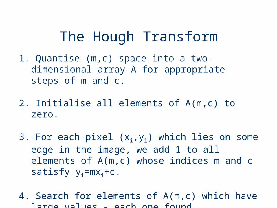
The Hough Transform1. Quantise (m,c) space into a two-dimensional

array A for appropriate steps of m and c.

2. Initialise all elements of A(m,c) to zero.

3. For each pixel (xi,yi) which lies on some edge in the image, we add 1 to all elements of A(m,c) whose indices m and c satisfy yi=mxi+c.

4. Search for elements of A(m,c) which have large values - each one found corresponds to a line in the original image.

The Hough Transform

0 0 0 0 0 0 0 0 0 0

0 0 0 0 0 0 0 0 0 0

0 0 0 0 0 0 0 0 0 0

0 0 0 0 0 0 0 0 0 0

0 0 0 0 0 0 0 0 0 0

0 0 0 0 0 0 0 0 0 0

0 0 0 0 0 0 0 0 0 0

0 0 0 0 0 0 0 0 0 0

0 0 0 0 0 0 0 0 0 0

0 0 0 0 0 0 0 0 0 0

y

x

m

c

0 1 0 0 0 0 0 0 0 0

0 0 1 0 0 0 0 0 0 0

0 0 0 1 0 0 0 0 0 0

0 0 0 0 1 0 0 0 0 0

0 0 0 0 0 1 0 0 0 0

0 0 0 0 0 0 1 0 0 0

0 0 0 0 0 0 0 1 0 0

0 0 0 0 0 0 0 0 1 0

0 0 0 0 0 0 0 0 0 1

0 0 0 0 0 0 0 0 0 0

0 1 0 0 0 0 0 0 0 0

0 0 1 0 0 0 0 0 0 0

0 0 0 1 0 0 0 0 0 0

0 0 0 0 1 0 0 0 0 0

0 0 0 0 0 1 0 0 0 0

1 1 1 1 1 1 2 1 1 1

0 0 0 0 0 0 0 1 0 0

0 0 0 0 0 0 0 0 1 0

0 0 0 0 0 0 0 0 0 1

0 0 0 0 0 0 0 0 0 0

0 1 0 0 0 0 0 0 0 0

0 0 1 0 0 0 0 0 0 0

0 0 0 1 0 0 0 0 0 1

0 0 0 0 1 0 0 0 1 0

0 0 0 0 0 1 0 1 0 0

1 1 1 1 1 1 3 1 1 1

0 0 0 0 0 1 0 1 0 0

0 0 0 0 1 0 0 0 1 0

0 0 0 1 0 0 0 0 0 1

0 0 1 0 0 0 0 0 0 0

m’

c’There is one line: y = m’x + c’

0 1 0 0 0 0 0 0 0 0

0 0 1 0 0 0 0 0 0 0

0 0 0 1 0 0 0 0 0 1

0 0 0 0 1 0 0 0 1 0

0 0 0 0 0 1 0 1 0 0

1 1 1 1 1 1 3 1 1 1

0 0 0 0 0 1 0 1 0 0

0 0 0 0 1 0 0 0 1 0

0 0 0 1 0 0 0 0 0 1

0 0 1 0 0 0 0 0 0 0

A Real Example

Image Edges

Accumulators Result

Another Parameter Space• Another equation for a straight line

= x.cos() + y.sin()

• For an n x n image- is in range [0, 2n]- is in range [0, 2]

• Each xi, yi generates a sinusoid in , space

Circles• Parametric equation is r2 = (x-a)2 + (y-b)2

- full problem cones in (a, b, r) space- known r circles in (a,b) space

Other Segmentation Methods

• Texture segmentation• Region growing

methods• The split and merge

algorithm• Motion segmentation

Texture Segmentation

• Another cue used in segmentation is image ‘texture’– texture is the local

variation in an image– even images with the

same overall intensity can look quite different

Carpet

Notice board

Wall

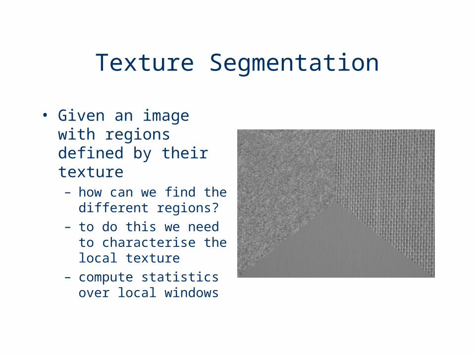
Texture Segmentation

• Given an image with regions defined by their texture– how can we find the

different regions?– to do this we need to

characterise the local texture

– compute statistics over local windows

Characterising Texture

• Textures can be quite complex– regular or random– small or large scale– with varying contrast

differences

• Simple statistics can help in some cases– there are more

complex methods

• We will use a local (11×11) window to compute– the average local

pixel value– the standard

deviation of the pixel values

Characterising Texture

• Given a set of n pixel values p1…pn we have

n

1i

2ip

n

1ii

)p(pn

1σ

pn

1p

Mean

Std. Dev.

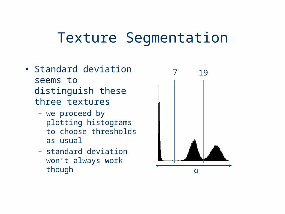
Texture Segmentation

• Standard deviation seems to distinguish these three textures– we proceed by

plotting histograms to choose thresholds as usual

– standard deviation won’t always work though

σ

7 19

Texture Segmentation

• The two thresholds define three regions– these correspond

closely to the texture regions

– some errors are made, especially at the boundaries

Region Growing

• Region growing starts with a small patch of seed pixels1. compute statistics

about the region2. check neighbours

to see if they can be added

3. if pixel(s) added, recompute the statistics and goto 2

• This procedure repeats until the region stops growing– simple example: We

compute the mean grey level of the pixels in the region

– neighbours are added if their grey level is near the average

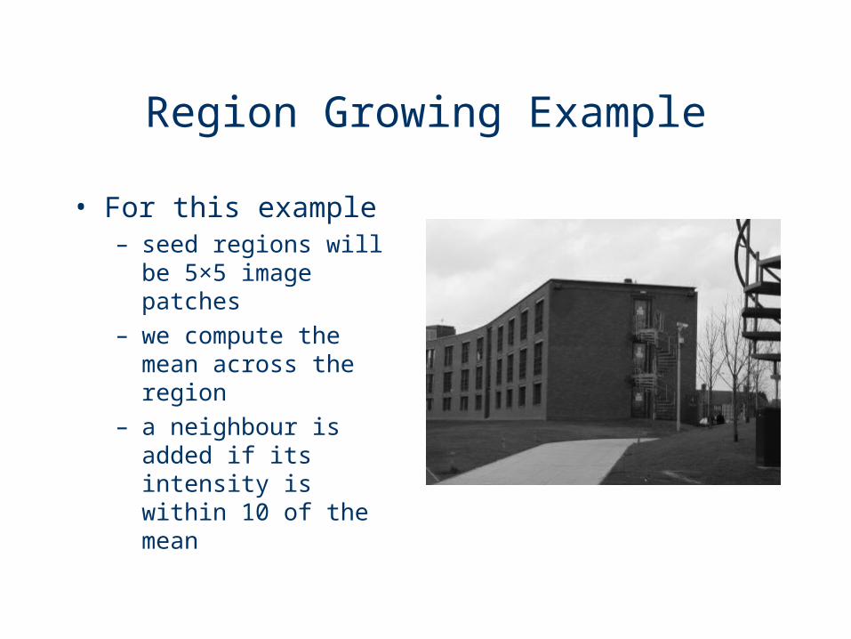
Region Growing Example

• For this example– seed regions will be

5×5 image patches– we compute the mean

across the region– a neighbour is added

if its intensity is within 10 of the mean

Region Growing Example

Region Growing

• Since all pixels belong to a region, any pixel may be selected and it will be part of some region

• The following pseudocodes can be used for segmenting the whole image:1. While there are pixels in the image that have not

been assigned to a region, select an unassigned pixel and make it a new region. Initialise the region’s properties.

2. If the properties of a neighouring pixel are not inconsistent with the region:2.1 add the pixel to the region2.2 Update the region’s properties2.3 Repeat from 2 using the updated properties

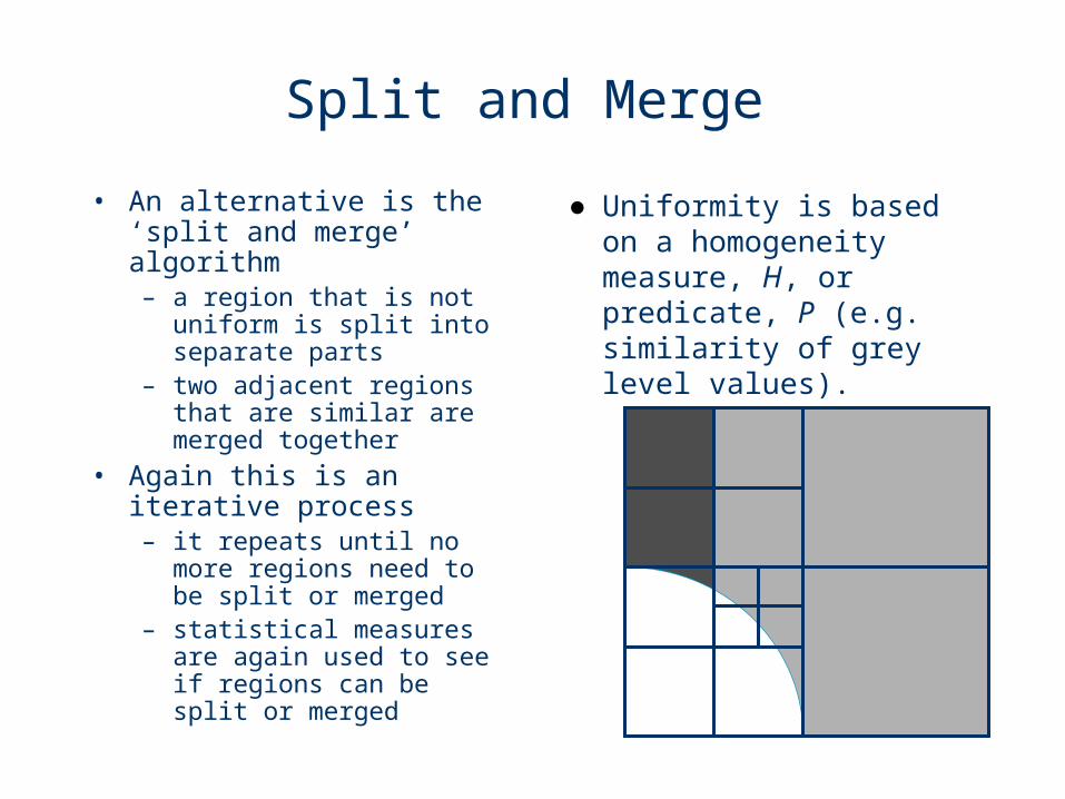
Split and Merge

• An alternative is the ‘split and merge’ algorithm– a region that is not

uniform is split into separate parts

– two adjacent regions that are similar are merged together

• Again this is an iterative process– it repeats until no more

regions need to be split or merged

– statistical measures are again used to see if regions can be split or merged

● Uniformity is based on a homogeneity measure, H, or predicate, P (e.g. similarity of grey level values).

● The main problem with region splitting is determining where to split a region.

● One method to divide a region is to use a quadtree structure.● Quadtree: a tree in which nodes have exactly four

descendants.

Region Splitting

Region Merging• Using the homogeneity condition or predicate definition

below, merge together all sub-regions where P(Rj U Rk) = TRUE.

• Can merge nodes of the tree that are not adjacent or on the same level.

• Can have an adaptive homogeneity condition.

Predicate definition

P = TRUE if σ > 10 AND 0 < µ < 125

P = FALSE otherwise

Splitting and Merging: Example

• Quadtree and RAG (region adjacency graph)

Motion Segmentation

• Up to now we have considered single images– often we have a

sequence of images of a scene

– motion detection is a useful way of finding objects

• The basic plan– take two (or more)

consecutive images of a scene

– look for differences between these images to detect motion

– group moving areas into objects

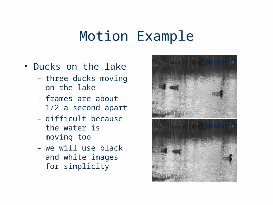
Motion Example

• Ducks on the lake– three ducks moving

on the lake– frames are about 1/2

a second apart– difficult because the

water is moving too– we will use black and

white images for simplicity

Frame 1

Frame 2

The Difference Image

• The difference in intensity between the two images– this might be positive

or negative so we can use

– or use a mid grey as representing 0, dark as +ve, light as -ve

y)(x,Iy)(x,Iy)D(x, 21

10055

Finding Moving Areas

• The moving areas seem quite clear– We can try and find a

threshold to separate them out

– As before we look at the histogram to find a good threshold value

– Neither value seems very clear, but we can try them out

– The problem is that the ducks are small and there is noise from the ripples on the water

T=55

T=100

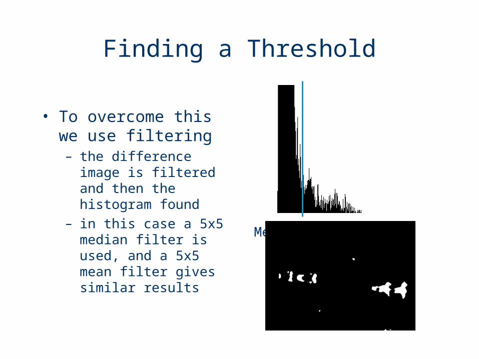
Finding a Threshold

• To overcome this we use filtering– the difference image

is filtered and then the histogram found

– in this case a 5x5 median filter is used, and a 5x5 mean filter gives similar results

Median filtered

Seeing Double

• Each moving object gives two regions in the motion image– one in areas where

the object is in frame 1, but not in frame 2

– one in areas where the object is in frame 2, but not in frame 1 duck in

frame 1duck inframe 2

Seeing Double

• These pairs of areas generally have opposite signs in the difference image– a dark object moving

on a light surface has a negative area in front of the motion, and a positive area behind

Frame 1

Frame 2

Difference

Acknowlegements

Slides are modified based on the original slide set from Dr Li Bai, The University of Nottingham, Jubilee Campus plus the following sources:

• Digital Image Processing, by Gonzalez and Woods