introduction to gis spatial analysis

OpenYourMineMaster Education Project Dedicated to Mineral Resources and Sustainability

Lisbon, 28.10.2019

Introduction to GIS spatial analysis

Dr. Jan Blachowski, WUST Prof.Department of Mining and Geodesy, WUST

2


Source: https://pl.m.wikipedia.org/wiki/Plik:Politechnika_Wroclawska_-_budynek_glowny.jpg

Source: http://www.pryzmat.pwr.edu.pl/wiadomosci/1013Source: http://www.pwr.edu.pl

3


Plan of lecture

• GIS data model

• Sources of GIS data

• Types of spatial analysis problems

• Spatial analysis concept

• Exmples of raster and vector functions and operations (approach to spatial analysis)

4


GIS DATA MODEL

Lat 66° 30' 11.0124'' NLong 25° 43' 37.0812'' E

Weather station

-8 °C2.5 m/s NE1010 hPa0 mmSunny

28.11.2019

5


GIS DATA MODEL

REAL WORLD

LANDUSE

ELEVATION

PARCELS

STREETS

CUSTOMERS

…

Source: https://peiyunprocess.wordpress.com

6


GIS DATA MODEL

• Real world objects, processes, phenomena, events, …REALITY

• Model of representation of objects, processes, phenomena representing a given domain, field or problem,

• Basic types of models: discrete object data model, continuous field data model

CONCEPTUAL MODEL

• Representation of the real world independent of the implementation environment,

• Basic type of models: raster data model, vector data modelLOGICAL MODEL

• Specifies file structure used for data storage,• Specific for a given environment of implementation (eg.

shapefile ESRI)PHYSICAL MODEL

7

• the type of analysis that can be performed in GIS depends on how the real world is represented(what data model is adopted),

• the adopted data model is of key importance for the implementation of the GIS project,• GIS is used in various organizations for different purposes – there is no universal data model


GIS DATA MODEL

source: Longley et al., 2005

8


RASTER DATA MODEL VS. VECTOR DATA MODEL

Discrete objects <> vector data model

Continuous fields objects <> raster data model

9


RASTER DATA MODEL

Raster characteristics

• Uses pixels (orthogonal cells) to represent data,• Pixels are organised in rows and columns,• Pixel size determines spatial resolution of data,• Pixels store value (integer or floating point),• Bit size determines range of values raster cell can represent

• 2 bit raster = 4 combinations: 00, 01, 10, 11• 4 bit raster = 16 combinations• 8 bit raster = 256 combinations• …• 32 bit raster = ?

10


RASTER DATA MODEL

Integer value raster, e.g. landuse Floating point raster, e.g. DEM, slope

Raster characteristics

Integer value raster• stores integer number or code• Value attribute table

Floating point raster• stores floating point numbers• Does not have value attribute table• Each value can be unique

11


RASTER DATA MODEL

RASTER SPACE COORDINATE SYSTEM SPACE

X’

RASTER LOCATION (x, y)

CELL SIZEROW

S

ROWS 6COLUMNS 8

Raster space determined by:• Number or rows and columns,• Size of pixel (cells)• Coordinate system space• Reference coordinates (x, y coordinates of raster origin)

Cells in a raster have unique position related to the origin of the raster

Y’

12


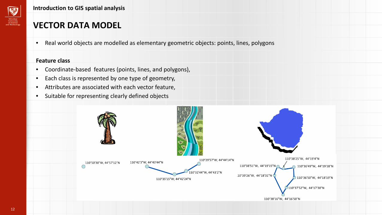
VECTOR DATA MODEL

• Real world objects are modelled as elementary geometric objects: points, lines, polygons

Feature class• Coordinate-based features (points, lines, and polygons),• Each class is represented by one type of geometry,• Attributes are associated with each vector feature,• Suitable for representing clearly defined objects

13


VECTOR DATA MODEL

Example - database of topographic objects

Figure 13. Visualization of Database of Topographic Objects

14


VECTOR DATA MODEL

Example – Mine map

• CAD data, Topology is important (connectivity and adjacency rules)

15


SOURCES OF GIS DATA

• Primary and secondary sources of data,• e.g. GNSS measurements (primary), cartographic documentation (secondary)

16


SOURCES OF GIS DATA

• Facebook?, Internet databases?• Used for pattern recognistion,• Rank of scientific centres

Figure 16. Visualization of scientific cooperation based on the Scopus database

Source Olivier H. Beauchesne, 2014 @http://olihb.com/2014/08/11/map-of-scientific-collaboration-redux/

17


DEFINITION OF GIS

EQUIPMENT

SOFTWAREDATA

PEOPLE METHODS

INTERNET

• There is also scientific disciple GIScience (geographic information science) (Goodchild, 2010)

18


GOOD AT SOLVING SPATIAL PROBLEMS

LOCATION

CONDITIONS

TRENDS

PATTERNS

IMPLICATIONS

19



LOCATION

CONDITIONS

TRENDS

PATTERNS

IMPLICATIONS

20



LOCATION

CONDITIONS

TRENDS

PATTERNS

IMPLICATIONS

Source: https://blogs.agu.org/fromaglaciersperspective/files/2017/10/klinaklini-compare-2017.jpg

21



LOCATION

CONDITIONS

TRENDS

PATTERNS

IMPLICATIONS

22



LOCATION

CONDITIONS

TRENDS

PATTERNS

IMPLICATIONS

23

How to apply analysis to solve spatial problems?


SPATIAL ANALYSIS CONCEPT

FRAME QUESTION

EXPLORE DATA

CHOOSE METHOD

PERFORM ANALYSIS

EXAMINE RESULTS

SHARE RESULTS

Explore data• Accuracy,• Scale,• Format,• Projection,• Availability,• Topicality,

Choose method• Identify tools,• Analyse

commonapproaches,

• Suitable data,• Break down

question,• Choose

functions

Perform analysis• Automate

procedures,• Code

procedures,• Model and

documentworkflow,

• Pilot analysis

Examine results• Examine

visually,• Examine

statistically,

Share results• Choose

presentationmethod,

• Share online• Static,

interactive

Framequestion• Define

problem to be solved

24


SPATIAL ANALYSIS FUNCTIONS OVERVIEW

• Map overlay and weighted map overlay concept

Source http://roopurbandesignseminar.blogspot.com/2016/10/design-nature-and-influence-ian-mcharg.html

Ian McHarg,Design with nature, 1969

Figure 24. Site analysis concept

25



• Polygon overlay (vector overlay)

Source http://wiki.gis.com/wiki/index.php/Overlay

Landuse

Underground water reservior

Union (OR)

Forest

Agriculture

Intersect (NOT)

Forest

Agriculture

Underground water reservior

Landuse

26



Spatial join (vector overlay)

• adds attributes of one feature class to another based on the spatial relationships between them

• Results depende on the spatial relationship defined for the procedure (intersect, are contained by, within a distance, etc.)

Targetfeatures

Appendedfeatures

Result for intersect

Result for within a specified distance

27





• Results depende on the spatial relationship defined for the procedure (intersect, are contained by, within a distance, etc.)

Targetfeatures

Appendedfeatures

Attribute rules

• Statistics can be calculated (sum, mean, max., min, first, last)

• Example (3 appended fetures with attribute value 10, 20, 30)

• SUM = 60• FIRST = 10• LAST = 30• MAX = 30• MEAN = ?

28





Targetfeatures

Appendedfeatures

Resources and production of dimension stones and crushed rocks in administrative units

29


MAP ALGEBRA (RASTER CALCULATOR)

Map Algebra Concept by Dana Tomlin 1990

Assumptions• Space can be divided into regular orthogonal units (cells),• Cell or cells can be subjected to specific, general and basic

transformations,• Transformations can be combined into sequences (as in

algebra) to form complex functions,• The data subjected to operations are treated as spatial

variables.

http://arcg.is/2vTfavQ

http://arcg.is/2vTfavQ

30



Map Algebra syntax

• Objects (raster data, values, tables),• Actions (operators and functions),

Operators - perform mathematical operations on or between data,Functions - cartographic modeling tools analyzing data made of cells (local, zonal, neighbourhood, central, …)

• Qualifier (parameters controlling action)

Raster 1

SUM: Raster 1 + Raster 2 = Raster 3

Raster 2 Raster 3

OPERATOR OBJECT

31



Map Algebra Map overlay

Point in Polygon Example

0 0 0 0

1 0 1 0

0 0 0 0

0 1 0 0

0 0 0 0

0 0 10 10

0 0 10 10

0 10 10 10

0 0 0 0

1 0 11 10

0 0 10 10

0 11 10 10

1 – Sample location(pollution),

0 – Remaining area

ResultLand useObservation points

10 – Agriculture0 – other types oflanduse

0 – Not sample location and not agriculture

1 – Sample location but not agriculture

10 – Use for agriculture but not sample location

11 – Sample location and use for agriculture

32



Map Algebra Map overlay

Polygin in Polygon Example (logical opertion)

1 – Permeable grounds0 – Remaining area

1 – Agriculture0 – other types oflanduse

0 – Non permeable grounds and not agriculture

1 – Permeable grounds or agriculture2 – Permeable grounds and agriulture

1 1 1 1

1 1 1 1

0 0 0 0

0 0 0 0

0 0 0 0

0 0 1 1

0 0 1 1

0 1 1 1

1 1 1 1

1 1 2 2

0 0 1 1

0 1 1 1

ResultAgriculturePermeable

grounds

33



Map Algebra functions

Local functions• The resulting raster cell value at a specific location is a function of the values of all input rasters (one or more)

for this location

• Example aplications– Calculating statistics for the location of each cel in a set of rasters,– Calculating the number of times the input raster values meet a given criterion,– Identification of values meeting the given criterion,– Identification of raster position in a set of raster data based on a given criterion,– Assigning unique values for each unique combination of values of two or more rasters.

34




Local functions• Example - calculating statistics for the location of each cell in a set of rasters

(sum, maximum, minimum, average, median, standard deviation, range, number of unique values, rank, …)

• Median,– Value separating the higher half from the lower half of a values in a given position of a set of rasters

– If number of input rasters is even then result is the average of two middle values,

Source: ESRI ArcGIS Help

Raster 1 Raster 2 Raster 3 Result Raster

35






• Range,– Calculates range of values for a given position in a set or input rasters

– Result can be floating point or integer raster,



36




• Highest Rank,– Returns the position of the raster containing the maximum value for a given position in the inputset of rasters

– What is the value of cell marked in red?





37






• Highest Rank,– Returns the position of the raster containing the maximum value for a given position in the inputset of rasters

– What is the value of cell marked in red? NO DATA



38




Zonal functions• perform operations on all cells belonging to a given zone

• A zone is an area consisting of cells with the same values• A zone can consist of several regions or unconnected cells

• A region is any group of connected (adjacent) cells in a zone

Examples of zonal functions• Zonal Geometry,• Zonal Statistics,• Functions determining the distribution of values in zones,• Funtions determining area of classes in zones,

Zone with value 42

Zone with value 44

Zone with value 46

Zone with value 50

Zone with value 48

Zone with value 52

Zone with value 54

Zone with value 58

39




Zonal geometry functions• perimeter,• area,• centroid

Perimeter

Input Raster Output Raster Input Raster Output Raster

Area

Input Raster Output Raster

Centroid

Angle of orientation

Major Axis

Minor Axis


40




Zonal statistics functions• The statistics are calculated for each zone specified in the input data set for the values of

the second data set (raster),• Statistics: sum, maximum, minimum, mean, median, range, minority, majority, standard

deviation, …

Zone Raster Output RasterValue Raster

Mean


41




Zonal histogram functions• Calculates distribution of values of the analysed feature in zones for input, zone and value

rasters

Example applications• Slope distribution in land cover classes,• Distribution of precipitation in elevation classes


42




Zonal histogram functions• Calculates distribution of values of the analysed feature in zones for input, zone and value

rasters

Example applications• Slope distribution in land cover classes,• Distribution of precipitation in elevation classes

Figure 42. Distribution of eco-environmental vulnerability (Nguyen, Liou, 2019)

43

Neighbourhood functions (Block statistic functions)• Calculates statistics for input raster cells in a specified neighborhood,• Statistics are calculated for all cells in a given neighborhood,• Neighbourhood can be user defined



1. Definition of Neighbourhood

RADIUS BLOCK #1

2 .Definition of Block (based on neighbourhood)

3 .Division of raster into Blocks 4. Calculation of values for each block

BLOCK #1 BLOCK #2 BLOCK #3INPUT RASTER OUTPUT RASTER

44


MAP ALGEBRA SURFACE ANALYSIS (VIEWSHED)

Parameters for calculation

• SPOT – DEM,• OF1 – offset, height of observation point above the

ground surface,• OF2 – offset, height added to raster cells representing

topographic features,• AZ1 – azimuth, initial angle of analysis, default value 0

degrees,• AZ2 – azimuth, end angle of analysis, default value 360

degrees, • V1 – initial vertical angle of analysis, default value 90

degrees,• V2 – end initial vertical angle of analysis, default value

90 degrees,• R1 – initial radius of analysis, default value 0 map units,• R2 – end radius of analysis, default value ∞ map units,

R2 > R1


45











R2 > R1

Source: https://pro.arcgis.com/en/pro-app/tool-reference/3d-analyst/viewshed-2.htm

Azimuth 1

Azimuth 2

Radius 1

Radius 2

Area of viewshedanalysis

46











R2 > R1

Source: Kowalczyk P., 2015

Visibility analysis ofr part of Highway (HWY-1) in Afganistan, Buckeye platform

47


MAP ALGEBRA SURFACE ANALYSIS (CUT AND FILL)

2010

2019

Deposition

Excavation

Suitable for analysis of processes during which the surface of the areahas been transformed as a result of excavation or deposition of material(anthropogenic, natural)

Example applications:

• calculation of the volume of material excavated and/or stored during construction or mining works,

• identification of subsidence areas in mining grounds,

• analysis of iceberg retreat processes,

• identification of areas prone to landslides,

• analysis and identification of erosionand deposition processes

48




Rasters need to be spatially congrugent(Resampling)

DEMinitial state

DEMEnd state

OutputNet change

Cell volume = Cell area x ΔZ

ΔZ = Zinitial – Zfinal

Source: ArcGIS Desktop Help

49




Deposition

Erosion

Source: http://www.et-st.com

50


PROXIMITY FUNCTIONS (vector approach)

Input polygonfeature

Output bufferfeatures

Output buffer feature includingarea of source feature

Multibuffer zones

• Buffering

d = 200

d = 400

Input line feature Output buffer feature Output buffer feature(selected side)

51



Input point feature Output bufferfeatures

Output buffer features (dissovlefunction applied)

• Buffering

d = 1000

d = 500

Output buffer features (attributeused)

52



• Buffering (example application)

railways

Crushed rock loading points

53




railways


Buffer zone, 1000m yellow2000m green

54




railways


Quarries usingroad transport

Buffer zone, 1000m yellow2000m green

55



• Near (different approach)


QuarriesRailways

• Distances calculated between all points of the input feature class and the nearest objects in the second feature class (based on the given search radius),

• Vector coordinates used

56


PROXIMITY FUNCTIONS (raster approach)

Euclidean distance

Input data (start points) Euclidean distanceraster

Start points

Start point 1

57


PROXIMITY FUNCTIONS (raster approach)

Euclidean distance

• Uses the node/link cell representation used in graph theory,

• Each center of a cell is considered a node and each node is connected to its adjacent nodes by multiple links,

• Links may have cost associated to them

Start point (cost 1)d1End point (cost 2)

Start point (cost 1)d1End point (cost 2)

𝒅𝒅𝒅𝒅 =𝒄𝒄𝒄𝒄𝒄𝒄𝒄𝒄 𝒅𝒅 + 𝒄𝒄𝒄𝒄𝒄𝒄𝒄𝒄 𝟐𝟐

𝟐𝟐 𝒅𝒅𝒅𝒅 =𝒅𝒅.𝟒𝟒𝒅𝒅𝟒𝟒 × (𝒄𝒄𝒄𝒄𝒄𝒄𝒄𝒄 𝒅𝒅 + 𝒄𝒄𝒄𝒄𝒄𝒄𝒄𝒄 𝟐𝟐)

𝟐𝟐


58


COST PATH

Euclidean distance

2 3 4

Raster of start points

Raster of costsurface

• Source cells (start points) are assigned value of 0 (2)• Cost of movement from source cells to adjacent cells is calculated (2)• Cell with the lowest value is stored in the output raster of cost path (value 1.5 above)• Cost for cells adjacent to cel with the lowest value is calculated (values 6.4, 3.5 above)• Again, the next cell with lovest values is stored in the output raster of cost path (value 2.0 above)


59


COST PATH

Euclidean distance

• The process continues for next cells• Cell value may change and is replaced if the new one is lower than the value obtained in the previous step (11.0> 8.0 above ),

5 6 7 8


60


MINIMUM COST PATH

Least cost path

Raster of accumulated costExample individual costs:DEMSlopeLanduseWind direction/speed

Raster of direction of movingfrom each location to sourcecell along path of least cost

Least cost pathe.g. new quarry to closestroad

61


DENSITY ANALYSIS

Density analysis methods

POINT LOCATIONS GRID OF REGULAR REFERENCE UNITS (CELLS), E.G. QUADRATS, HEXAGONS

REFERENCE UNITS SUCH AS ADMNISTRATIVE DIVISIONS

DENISTY SURFACE

62


DENSITY ANALYSIS


Quadrat Count Methodsgeneralization of one-dimensional analysis (histogram) into a two-dimensional case

Point density• Calculates density of point features around each output raster cell.• neighborhood is defined around each raster cell center, and the number of points that fall within the

neighborhood is summed up and divided by the area of the neighborhood• Attribute values can be associated with point features

63


DENSITY ANALYSIS


Point density

Dimension stone and crushed rock deposits / quarries

Attribute reserves, production

Density of dimension stone and crushed rock deposits or quarriesDensity of reserves,

Density of output

2.5 visualisationChange in spatial distribution of the analysed

phenomenon

64


FUTURE TRENDS – Internet of Things (IoT, Industry 4.0)

Source https://blogs.3ds.com/geovia/part-2-iot-4th-industrial-revolution/

Figure 17. The Mining Internet of Things

65


SUMMARY

• GIS data model defines / affects geospatial analysis procedure,• Conversion and/or harmonisation of data may be necessary,

• Applications and case studies tomorrow

KNOWLEDGE

INFORMATION

DATA

66


FURTHER READING

• Berry J., 1989-2013: Beyond Mapping Compilation Series. GIS Modeling: Applying Map Analysis Tools and Techniques (columns from 2007 to 2013)

• Berry J., 1989-2013: Beyond Mapping Compilation Series. Map Analysis: Understanding Spatial Patterns and Relationships (columns from 1996 to 2007)

• DeMers M., 2005: Fundamentals of Geographic Information Systems. John Wiley & Sons,

• Duckham M. (Ed.), Goodchild M. (Ed.), Worboys M. (Ed.) 2003: Foundations of Geographic Information Science, CRC Press,

• Heywood I., Cornelius S., Carver S., 2006: An Introduction to Geographical Information Systems, 3rd Edition, Pearson – Prentice Hall,

• Kennedy M., 2013: Introducing Geographic Information Systems with ArcGIS: A Workbook Approach to Learning GIS, Third Edition, John Wiley and Sons,

• Longley P. A., Goodchild M. F., Maguire D. J., Rhind D. 2011: Geographic Information Systems and Science, John Wiley & Sons,

• Madden M. (Ed.), 2009: Manual of Geographic Information Systems, Acamedia

Thank you for your [email protected]

introduction to gis spatial analysis

Documents