introduction to gauss programming language -...
TRANSCRIPT

Introduction to GAUSS ProgrammingLanguage
Eduardo RossiUniversity of Pavia
September, 2004
Contents1 Introduction 5
2 Platforms and Interfaces 62.1 Memory management . . . . . . . . . . . . . . . . . . . . . . . 62.2 Interfaces . . . . . . . . . . . . . . . . . . . . . . . . . . . . . 7
3 Programming Tips 7
4 Layout and Syntax 8
5 The GAUSS Windows Environment 85.1 Startup Options . . . . . . . . . . . . . . . . . . . . . . . . . . 105.2 Running Commands Interactively . . . . . . . . . . . . . . . . 105.3 Command Keys . . . . . . . . . . . . . . . . . . . . . . . . . . 115.4 Function Keys . . . . . . . . . . . . . . . . . . . . . . . . . . . 125.5 Exercises . . . . . . . . . . . . . . . . . . . . . . . . . . . . . . 125.6 Running Commands from Files . . . . . . . . . . . . . . . . . 135.7 File Menu . . . . . . . . . . . . . . . . . . . . . . . . . . . . . 135.8 Edit Menu . . . . . . . . . . . . . . . . . . . . . . . . . . . . . 14
5.8.1 Bookmarks . . . . . . . . . . . . . . . . . . . . . . . . 145.9 Run Menu . . . . . . . . . . . . . . . . . . . . . . . . . . . . . 155.10 The Help system . . . . . . . . . . . . . . . . . . . . . . . . . 16
1

6 GAUSS Data Types 166.0.1 Examples of data types . . . . . . . . . . . . . . . . . . 186.0.2 Grouping variables . . . . . . . . . . . . . . . . . . . . 19
6.1 Creating matrices . . . . . . . . . . . . . . . . . . . . . . . . . 206.1.1 Creating a matrix using constants: LET . . . . . . . . 206.1.2 Examples of LET . . . . . . . . . . . . . . . . . . . . . 216.1.3 Creating a matrix using values . . . . . . . . . . . . . . 226.1.4 Examples of assigning values to a variable . . . . . . . 22
6.2 Referencing matrices . . . . . . . . . . . . . . . . . . . . . . . 236.2.1 Direct references . . . . . . . . . . . . . . . . . . . . . 236.2.2 Indirect references . . . . . . . . . . . . . . . . . . . . 266.2.3 Nested references . . . . . . . . . . . . . . . . . . . . . 27
7 Managing data - SHOW, PRINT, FORMAT, NEW, CLEAR,DELETE 287.1 SHOW . . . . . . . . . . . . . . . . . . . . . . . . . . . . . . . 287.2 PRINT and FORMAT . . . . . . . . . . . . . . . . . . . . . . 287.3 NEW, CLEAR, and DELETE . . . . . . . . . . . . . . . . . . 30
8 GAUSS procedures 32
9 Matrix algebra 359.1 The basic operators . . . . . . . . . . . . . . . . . . . . . . . . 35
9.1.1 Concatenation . . . . . . . . . . . . . . . . . . . . . . . 389.1.2 Conformability and the ”dot” operators . . . . . . . . 399.1.3 Relational operators and dot operators . . . . . . . . . 419.1.4 Fuzzy operators . . . . . . . . . . . . . . . . . . . . . . 42
10 Set operations 43
11 Special matrix operations 4311.1 Some useful matrix types . . . . . . . . . . . . . . . . . . . . . 4311.2 Special operations . . . . . . . . . . . . . . . . . . . . . . . . . 4411.3 Manipulating matrices . . . . . . . . . . . . . . . . . . . . . . 45
12 Examples 47
13 Manipulating Matrices 2 50
2

14 Mathematical Functions 54
15 Statistical Functions 56
16 Strings 58
17 Printing 59
18 Missing Values 62
19 Exercises 65
20 Flow of control 6720.1 Conditional branching: IF . . . . . . . . . . . . . . . . . . . . 67
20.1.1 IF examples . . . . . . . . . . . . . . . . . . . . . . . . 6920.2 Loop statements: WHILE/UNTIL and FOR . . . . . . . . . . 75
20.2.1 WHILE/UNTIL loops . . . . . . . . . . . . . . . . . . 7520.2.2 WHILE examples . . . . . . . . . . . . . . . . . . . . . 7620.2.3 FOR loops . . . . . . . . . . . . . . . . . . . . . . . . . 8320.2.4 FOR examples . . . . . . . . . . . . . . . . . . . . . . 8320.2.5 Exercises . . . . . . . . . . . . . . . . . . . . . . . . . . 85
20.3 Suspending execution: PAUSE, WAIT and END . . . . . . . . 8720.3.1 Temporary suspension using commands . . . . . . . . . 8720.3.2 Terminating a program using commands . . . . . . . . 87
21 Publication Quality Graphics 8921.1 Commands . . . . . . . . . . . . . . . . . . . . . . . . . . . . 9021.2 Global variables . . . . . . . . . . . . . . . . . . . . . . . . . . 9121.3 Fonts and Special Characters . . . . . . . . . . . . . . . . . . 9321.4 Windows . . . . . . . . . . . . . . . . . . . . . . . . . . . . . . 9721.5 Examples . . . . . . . . . . . . . . . . . . . . . . . . . . . . . 99
22 Input and Output 10422.1 GAUSS Matrices . . . . . . . . . . . . . . . . . . . . . . . . . 10422.2 ASCII files . . . . . . . . . . . . . . . . . . . . . . . . . . . . . 105
22.2.1 Reading . . . . . . . . . . . . . . . . . . . . . . . . . . 10522.2.2 Writing . . . . . . . . . . . . . . . . . . . . . . . . . . 108
22.3 Spreadsheets . . . . . . . . . . . . . . . . . . . . . . . . . . . . 10922.3.1 Format . . . . . . . . . . . . . . . . . . . . . . . . . . . 113
3

22.4 GAUSS Dataset . . . . . . . . . . . . . . . . . . . . . . . . . . 11722.4.1 Creating new datasets . . . . . . . . . . . . . . . . . . 11722.4.2 Opening datasets . . . . . . . . . . . . . . . . . . . . . 11922.4.3 Reading and Moving about . . . . . . . . . . . . . . . 12022.4.4 Writing . . . . . . . . . . . . . . . . . . . . . . . . . . 12022.4.5 Closing . . . . . . . . . . . . . . . . . . . . . . . . . . . 121
23 Procedures 12223.1 Global and local variables . . . . . . . . . . . . . . . . . . . . 12323.2 Writing procedures . . . . . . . . . . . . . . . . . . . . . . . . 12423.3 Global Variables in External Procedures . . . . . . . . . . . . 13023.4 Procedures as variables . . . . . . . . . . . . . . . . . . . . . . 131
24 Functions and keywords 135
25 Exercises 136
26 Procedures: examples 13726.1 Ordinary least squares . . . . . . . . . . . . . . . . . . . . . . 13726.2 Runge - Kutta Algorithm . . . . . . . . . . . . . . . . . . . . 14126.3 Simulation of Stochastic Differential Equation. Euler - Maruyama
Algorithm . . . . . . . . . . . . . . . . . . . . . . . . . . . . . 14526.4 Simulation of the price of a European Call Option . . . . . . . 14526.5 Monte Carlo Simulation to price a European Call Option . . . 14826.6 Simulation of Poisson Process . . . . . . . . . . . . . . . . . . 15026.7 Simulation of Diffusion Process with jumps . . . . . . . . . . . 153
4

1 IntroductionGAUSS is a complex language with a large number of specialised functionsfor dealing with matrices. There are also a lot of add-on packages whichexpand GAUSS’s capabilities further.The emphasis in this course is on acquiring familiarity with the funda-
mentals of GAUSS and programming competence, rather than becoming aGAUSS guru.
GAUSS is a programming language designed to operate with and on ma-trices. It is a general purpose tool. As such, it is a long way from morespecialised econometric packages. On a spectrum which runs from the com-puter language C at one end to, say, the menu-driven econometric programEViews at the other, GAUSS is very much at the programming end.
Advantages
1. GAUSS is appropriate for a wider range of applications than standardeconometric packages because it is a general programming language.
2. GAUSS operates directly on matrices. This makes it more useful foreconomists than standard programming languages where the basic dataunits are all scalars.
3. GAUSS programs and functions are all available to the user, and sothe user is able to change them.
4. Similarly, if data is held in a non-standard format, you may write yourown routine to access it.
5. GAUSS is extremely powerful for matrix manipulation. It is also fastand efficient.
Disadvantages
1. The fixed costs of using GAUSS are high. Its very generality meansthat there is unlikely to be a simple procedure to do a simple econo-metric task readily to hand (although commercially available routinesameliorate this somewhat).
5

2. Even if pre-programmed or bought in software is available for a task,a reasonable degree of familiarity with GAUSS and its methods willoften be necessary to make effective use of such routines.
3. GAUSS is too tolerant of sloppy programming. GAUSS is very flexible;however, this means it is difficult for the computer to tell when mistakesoccur. For example, lax conformability requirements mean that it iseasy to mistakenly divide a scalar by a row vector and then multiplyby a matrix in the belief that all three variables were column vectors.
4. GAUSS is not tolerant of errors in its environment. Ask it to readfrom a non-existent file, or use an uninitialised variable, and the pro-gram stops. This is, of course, a sensible feature of all programminglanguages. Unfortunately, GAUSS is short on routines allowing non-fatal error checking.
5. Input and output routines are basic - especially input.
6. GAUSS programs are designed to be run within the GAUSS environ-ment. They cannot be run as stand-alone programs (.EXE files) with-out buying a program called the GAUSS ”Run-time Engine”TM. Thusyou can only swap code with other GAUSS users.
2 Platforms and InterfacesGAUSS is available in both single user versions and networked versions.GAUSS on Unix is very powerful and very quick, partly because Unix
machines are designed for heavy-duty processing and computation ratherthan user interaction. For manipulating large matrices, the time saving canbe tremendous.GAUSS on Unix runs in both teletype (command-line) and X-Windows
mode. Access to the latter depends on how you access your Unix machine.There is also a version to run on Linux (a form of Unix which runs on
Intel processors).
2.1 Memory management
In the early days of GAUSS, efficient memory management was often crucialto getting a program running well. The amount of memory used by GAUSS
6

could be varied by the user to make appropriate use of scarce resources.However, this is much less of an issue in modern computers, and from version4.0 for Windows, GAUSS no longer gives you the option to manage memorydirectly. Instead it relies on the more efficient memory-management facilitiesof the operating system.
2.2 Interfaces
GAUSS programs can be written in two ways:
• command-lineIn this mode, commands typed into the GAUSS interface are executedimmediately. This allows for an instant response to a command, but thecommands cannot be stored. This is therefore not suitable for writinglarge programs, or for commands which need to be run repeatedly.
• batch or programIn this mode, GAUSS commands are typed into a text file. This fileis then sent to be GAUSS to be run. This allows one to develop andstore complex programs.
This facility has existed since the earliest versions of GAUSS. However,the precise way this is carried out has varied over time. The original DOSinterface is still extant in the latest Windows version as ”TGAUSS”, butthe recommended interface is the windowing one. The Unix version is closerto the DOS version but has a few operating differences. Additionally, allthree versions draw graphics windows differently as a result of their operatingenvironments.
3 Programming TipsYour programs will be easier for others to follow and revise if you follow somesimple tips:
1. Clean code means that do loops are indented
2. Clean code means that comments are liberally used, allowing readersto follow the program’s logic.
7
3. A block of comments may be enclosed between two @ symbols or be-tween /* and */. Comments delimited by the /*, */ symbols may benested. Comments delimited by the @ symbol may not be nested. Inaddition, comments on a single line may be preceded by //
4. Clean code means using spaces liberally, and not necessarily includingas many operations as possible in a single line of code.
4 Layout and SyntaxGAUSS could be described as a free-form structured language: structuredbecause GAUSS is designed to be broken down into easily-read chunks; free-form because there is no particular layout for programs. Although the syntaxis closely defined, extra spaces between words (including line breaks) areignored. Commands are separated by a semi-colon, rather than having onecommand on each line as in FORTRAN or BASIC. A complete instruction isidentified by the placing of semicolons, and not by the placing of commandson different lines.Program layout is generally a matter of supreme indifference to GAUSS,
and this gives the user freedom to lay out code in a style he finds acceptable.GAUSS is not case-sensitive.
5 The GAUSS Windows Environment• Start GAUSS for Windows.• You will see the GAUSS menu bar, the GAUSS toolbar, the workingdirectory toolbar, a Command Input-Output window and, near or atthe bottom of the screen, the GAUSS status bar.
• Your cursor will be in the Command Input-Output window, next to aGAUSS prompt, >>, in the lower left corner of the screen.
GAUSS runs the le startup when it starts. Often users put a chdir com-mand in the startup le to change the GAUSS working directory.GAUSS starts up with the same con guration it had when last shutdown.
Main windows in GAUSS for Windows include:
8

the Command Input-Output
Edit
Output
Debug windows
Additional windows include a Matrix Editor window and an HTML Helpwindow.
Code may be run from the:
Command Input-Output window
Edit window.
Output may appear in the:
Command Input-Output window
Output window
sent to a file.
Command Input-Output Window. Enter interactive commands andview output in the Command Input-Output window. Give this window focusby clicking inside it, by selecting it from the Windows Menu, or by typingCtrl+W.
Edit Window. Edit windows are created and opened a number of ways.
Click the New button on the toolbar.
Type edit filename from the GAUSS prompt. This opens a new Edit windowif filename does not already exist in the current directory. For example,typing
edit c:\mydir\myfile.srcopens c:\mydir\myfile.src for editing.It will reside in the c:\mydir directory when saved.
9
Type
edit filename
from the GAUSS prompt. This opens the the editor for an existing fileif filename already exists.
Click the File/New menu combination.
Output Window. Output is written to the Output window when it isactive. GAUSS commands cannot be executed from the Output window. TheOutput window is made active and inactive by selecting it from the GAUSSWindow menu, or by using the keyboard shortcut Ctrl+O. Note that Ctrl+Ohas two functions. It gives the Output window focus and changes its state(active/inactive).
Debug Window. The Debug window and Debug toolbar are displayedduring a debugging session.
5.1 Startup Options
Startup options are set in the GAUSS installation directory’s startup fileor using the Configure/Preferences and Configure/Editor Properties menuitems. GAUSS starts with the preferences that were in place when it waslast shutdown.Each window, including each Edit window, has its own set of options.
This means that you will need to configure each window independently.
5.2 Running Commands Interactively
Single commands or blocks of commands may be run interactively from theCommand Input-Output Window.Select the Command Input-Output window by clicking inside it or by
typing Ctrl+W.Move to the bottom by scrolling or by simply typing Ctrl+End. You will
see the GAUSS prompt.Interactive commands are typically entered at the GAUSS prompt. When
you run commands interactively, the processed code lies between the GAUSSprompt and the end of the current line. This is called the active block .
10

The active block can be one or more lines of code.Pressing Ctrl-I will insert a GAUSS prompt in your code. This is often
useful when you want to start a new active block from the middle of a line.Enter an active block with more than one line of code into the Command
Input-Output window by pressing CTRL+Enter at the end of each line. Atthe end of the final line press Enter.A block of commands may be executed by selecting the code and dropping
it into the Command Input-Output window next to the GAUSS prompt, byclicking the Run Selected Text button, or by typing Ctrl+R.Repeat the last command line by pressing CTRL+L.
5.3 Command KeysCTRL+A RedoCTRL+C Copy selection to the Windows clipboardCTRL+D Open the Debug windowCTRL+E Open the Matrix EditorCTRL+F Find/Replace textCTRL+G Go to the speci ed line numberCTRL+I Insert the GAUSS promptCTRL+L Insert lastCTRL+N Make the next window activeCTRL+O Open the Output window and change its stateCTRL+P Print the current window, or selected textCTRL+Q Exit GAUSSCTRL+R Run selected textCTRL+S Save the window to a leCTRL+W Open the Command windowCTRL+V Paste the contents of the Windows clipboardCTRL+X Cut the selection to the Windows clipboardCTRL+Z Undo
11

5.4 Function KeysF1 Open the GAUSS Help system or context-sensitive HelpF2 Go to the next bookmarkF3 Find againF4 Go to the next search item in Source BrowserF5 Run the Main FileF6 Run the Active FileF7 Edit the Main FileF8 Step IntoF9 Set/Clear breakpointF10 Step OverALT+F4 Exit GAUSSALT+F5 Debug the Main FileCTRL+F1 Searches the active libraries for the source code of a function.CTRL+F2 Toggle bookmarkCTRL+F4 Close the active windowCTRL+F5 Compile the Main FileCTRL+F6 Compile the Active FileCTRL+F10 Step OutESC Unmark marked text
5.5 Exercises
1. Type some simple GAUSS commands in the GAUSS Command Input-Output window, e.g.:
let x = 1 2 3 4;
Print x;
2. Open the Output window. Notice that output appears in the Outputwindow when you type commands in in the Command Input-Outputwindow. Switch focus to the Output window by clicking in it or by usingthe keystroke shortcut, Ctrl+O. Switch focus back and forth betweenthe Command Input-Output and Output windows.
3. Tile the Command Input-Output and Output windows, either verticallyor horizontally by selecting a Tile option from the Window menu (hor-izontal tiling is often useful when GAUSS output is long horizontally).
12
Have the output from some simple commands display alternately in theCommand Input-Output and Output windows.
5.6 Running Commands from Files
The GAUSS for Windows environment distinguishes between two files, theActive file and theMain file. The Active file is often called the Currentfile.
The Active file is the one displayed in the Edit window, the one withfocus. An Active file may also be the Main file.
Execute the active file by clicking Run Active File on the Run menu,by clicking the Run Currently Active File button on the Main tool-bar, or by pressing F5.
A file must be saved to disk before it becomes the Active file.
TheMain file is displayed in the Main File list.
Execute theMain file by clicking Run Main File on the Runmenu, byclicking the Run Main File button on the Main toolbar, or by pressingF6.
Make an Active file the Main file by choosing the Run/Set MainFile menu item.
5.7 File Menu
Some useful items in the File menu are
Change Working Directory
Clear Working
Directory List
Recent Files.
Change Working Directory may also be implemented using a chdir orchangedir
13
command or by selecting a directory from the working directory toolbar.
The ten most recent files opened are displayed at the end of the File menu.If the file you want to open is on this list, click it and GAUSS opens itin an Edit window.
5.8 Edit Menu
Edit window items and associated keyboard shortcuts are:Undo Ctrl+ZRedo Ctrl+ACut Ctrl+XCopy Ctrl+CPaste Ctrl+VSelect AllClear AllFind Ctrl+F
The search can be case sensitive or case insensitive. You may also limitthe search to regular expressions.
Find Again F3Replace Ctrl+Alt+F3Insert Time/DateGo to Line Ctrl+GGo to Next Bookmark F2Toggle Bookmark Ctrl+F2Edit BookmarksRecord Macro Ctrl+Shift+R
5.8.1 Bookmarks
Bookmarks enable quick and easy cursor movement to particular lines orsections of code.
To add a bookmark, place the cursor in the line you want to bookmark andpress Ctrl+F2 or click the Toggle Bookmark item on the Edit menu.
Cycle forward through all bookmarks by pressing F2. Cycle backwardsthrough all bookmarks with Shift+F2.
14

The Edit Bookmarks window lets you add, remove, name, or jump to aparticular bookmark.
This window is opened when you select Edit Bookmarks from the Editwindow.
Margin display must be turned on to see bookmarks. Use the Misc tabin the Configure/Editor Properties menu to turn margins on and off.
5.9 Run Menu
The Run Menu is used to access run commands. Run Menu items are:
Insert GAUSS Prompt Keyboard shortcut: Ctrl+I
Manually adds a GAUSS prompt at the cursor position.
Insert Last Command Keyboard shortcut: Ctrl+L
Run Selected Text Keyboard shortcut: Ctrl+R
This is active only when text is selected.
Run Active File Keyboard shortcut: F6
Runs the active file.
Test Compile Active File Keyboard shortcut: Ctrl+F6
This is used to see whether the Active le will compile, without enteringsymbols into the symbol table.
Run Main File Keyboard shortcut: F5
Runs the Main file.
Test Compile Main File Keyboard shortcut: Ctrl+F5
This is used to see whether the Main le will compile, without enteringsymbols into the symbol table.
Edit Main File Keyboard shortcut: F7
Opens an editor window for the Main le. The le is loaded, if needed,and the Edit window becomes the active window.
15
Stop Program Stops a program while it is running. The program willstop only after nishing the currently active GAUSS command. Thissometimes takes considerable time, especially if the active commandinvolves optimization. In this case, closing GAUSS via the taskbar isthe only other way to stop the execution of a program.
Build GCG File from Main
Set Main File
Clear Main File List
Translate Dataloop Commands This must be checked if dataloop isbeing used.
5.10 The Help system
GAUSS has two electronic help systems, corresponding to the manuals. The”Command Reference” is an easy way to pick up information on commands(as long as they are not deemed ”obsolete”), and is organised both alphbet-ically and by function, which is useful. It is very terse and does not displayproperly, but generally seems accurate.The ”User Guide” is slightly more chatty, and has more examples. Note
however that it is less reliable. First, information on old commands is leftunchanged, even though the commands may operate in a different way inlater versions or has been deleted altogether. Second, information on newfunctions is often not forthcoming in that version. The first problem doesseem to be disappearing, but if something doesn’t work as the manual saysit should, don’t assume that it’s your code that’s wrong.
6 GAUSS Data TypesGAUSS has two data types:
• matrices• strings (or string arrays).
16

Matrices may contain numeric and character data; GAUSS does not dis-tinguish internally between the two. Both are stored as double precision (8byte) data.Numeric matrices and numeric matrix elements are printed to the
screen using a print command.Character matrix elements are limited in length to 8 characters.
Character matrix elements are printed to the screen using aPrint $variablename command.Strings are printed using aPrint variablename command.
Matrices obviously include vectors (row and column) and scalars as sub-types, but these are all treated the same by GAUSS. For example
a = b + c;
is valid whether a, b, and c are scalars, vectors, or matrices, assuming thevariables are conformable. However, the results of the operation may differdepending on the variable type.
Matrices may contain numerical data or character data or both.Eight bytes are used to store each element of a matrix. Hence, each cell ina matrix can contain up to eight text characters, or numerical data with arange of about 1.0E±35.If you enter text of more than eight characters into the cells in a matrix,
the text will be truncated.Numerical data are stored in scientific notation to around 12 places of
precision.
Strings are pieces of text of unlimited length. These are used to giveinformation to the user. If you try to assign a string value to an element ofthe matrix, all but the first eight characters will be lost.
17

6.0.1 Examples of data types
(4× 3) Numerical matrix 1 2.2 −38 88 100
3.11E − 6 −2 58.6E + 29 1000 2
(2× 4) Character matrix·
Will Jack Harry SteveLory Dick Mary John
¸(3× 3) Mixed matrix Milan 40 K
Rome 22 MLondon 1 N
Strings
’’Hello Mum!’’’’Strings are pieces of text of unlimited length’’’’2.2’’’’’’The null string ”” is a valid piece of text for both strings and matrices.
Because GAUSS treats all matrix data the same, GAUSS sometimes mustbe told that it is dealing with character data. The $ sign identifies text and isused in a number of places. For example, to display the value of the variable”v1” requiresPRINT v1; PRINT $v1;orPRINT v1;PRINT $v1;depending on whether v1 is a numerical matrix, a character matrix, or a
string. Strings are identified by GAUSS and don’t need the $. You can putone in if you like but it makes no difference to printing.
18

Variables need to have names to reference them. Names can be any length(except in very old versions of GAUSS where they must be eight charactersor less). Acceptable names for variables can contain alphanumeric data andthe underscore ”_”, and must not begin with a number. Reserved wordsmay not be used; standard procedure names may be reassigned, but this isnot generally a good idea. Variables names are not case-sensitive.
Acceptable variable names:eric Eric eric1 eric_1 _eric1 _e_r_i_cUnacceptable variable names:1eric 100 if (reserved word) delif (GAUSS procedure - legal, but fool-
ish)
Using good variable names can make a big difference to your program-ming. Having variables called ”m” and ”t” may be quick to write, but”max_value” and ”total_obs” would be more meaningful, and hence easierto interpret when you come back to look at a program later when you’veforgotten what it does.
6.0.2 Grouping variables
String arrays String arrays are, as the name suggests, a convenient wayof grouping strings. They are similar to a character matrix, but the stringsthey contain can be of unlimited length. Thus this is a valid string array: Mediobanca Italy
JPMorgan USASchroeder UK
Note how the data fields are more than eight characters long. One differ-
ence between a character matrix and a string array is that GAUSS treatsthe former as a standard array so you can carry out any matrix operationon it, whether it makes sense or not. In contrast, a lot of operations will notbe allowed on a string array because GAUSS ’understands’ the string datatype.String arrays are therefore more flexible in storing characters. However,
they have some disadvantages:
1. they only store strings, and therefore you cannot mix character andnumeric data.
19

2. because the length of the element is variable, GAUSS will handle themless efficiently. If all your character strings are eight characters or less,then keeping them in a character matrix may be marginally quicker.Third, string arrays take up more memory. For example, a 32768-element character matrix takes roughly 270Kb, irrespective of the num-ber of characters. A string matrix with an average string length of 4characters takes 400Kb; with an average length of eight characters thatrises to 560Kb, twice as much as the equivalent character matrix.
Structures Structures allow the grouping of variables of different types.They were introduced in version 4.0. Suppose you are running repeatedregressions and for each regression you want to store the following informationfor each array:Scalars: TSS, ESS, RSS, s, NVectors: Coefficients, standard errorsString array List of variable namesBy placing these into a structure, they could be passed around between
procedures, simplifying the program. This could also mean lower mainte-nance, by minimising changes to procedure calls if the structure form changes.
6.1 Creating matrices
New matrices can be defined at any point (except inside procedures). Theeasiest way is to assign a value to one. There are two ways to do this - byassigning a constant value or by assigning the result of some operation.
6.1.1 Creating a matrix using constants: LET
The keyword LET creates matrices. The format for creating a matrix calledvarName is
LET varName = constant-list;LET varName[r,c] = constant-list;
In the first case, the type of matrix created depends on how the constantswere specified.
A list of constants separated by space will create a column vector.
20

If, however, the list of constants is enclosed in braces {}, then a row vectorwill be produced.
When braces are used, inserting commas in the list of constants instructsGAUSS to form a matrix, breaking the rows at the commas, then an(r × c) matrix will be created; the constants will be allocated to thematrix on a row-by-row basis.
If curly braces are not used, then adding commas has no effect. In the firstcase, the actual word ’LET’ is optional.
If only one constant is entered, then the whole matrix will be filled withthat number.Note the square brackets. This is the standard way to tell GAUSS
either the dimensions of a matrix or the coordinates of a block, depending oncontext. The first number refers to the row, the second the column. Curlybraces generally are used within GAUSS to group variables together.
6.1.2 Examples of LET
Command Shape of x:
LET x = 1 2 3 4 5 6; Column vector (6× 1)LET x = 1,2,3, 4,5, 6; Column vector (6× 1)LET x = 1 2, 3 4, 5 6; Column vector (6× 1)LET x = {1 2 3 4 5 6}; Row vector (1× 6)LET x = {1,2,3, 4,5, 6}; Column vector (6× 1)LET x = {1 2, 3 4, 5 6}; Matrix (3× 2)LET x[3,2] = 1 2 3 4 5 6; Matrix (3× 2)LET x[3,2] = 1, 2, 3, 4, 5, 6; Matrix (3× 2)LET x[3, 2] = 5; Matrix (3× 2)
21

If we have two variables ”a” and ”b” then the commandLET x = a*b;is illegal as ”a*b” is a value and not a constant. In practice, GAUSS
will interpret ”a*b” as a string constant and will create a string variablecontaining the letters and figures ”a*b”.
6.1.3 Creating a matrix using values
The results of any operation can be placed into a matrix without an LETexplicit declaration. The result of the operation
m1 = m2 + m3;
will be that the value ”m2+m3” is contained in a variable called ”m1”. If thevariable m1 did not exist before this statement, it will have been created.The size and type of a variable depends entirely on the last thing done
with it. Suppose m1 existed prior to the last operation. If m2 and m3 are bothscalars, then m1 will now be a scalar - regardless of whether it was previouslya matrix, vector, scalar, or string.
Variables have no fixed size or type in GAUSS - they can be changed atwill simply by assigning a different value to them. It is up to the programmerto make sure he has the correct variable for any operation, as GAUSS willrarely check.Assigning a value is done by writing down the equation. Any correct (for
GAUSS’s syntax) mathematical expression is acceptable, as are strings orthe results of procedures.
6.1.4 Examples of assigning values to a variable
The routines ZEROS and ONES create matrices of 0s and 1s. The transposeoperator ’ can be used as in any normal equation. Examining the impact ofvarious assignment statements on matrices m1, m2 and m3 we get
22

Command m1 m2 m3
m1=ZEROS(2,3); (2× 3) undefined undefinedm2=ONES(1,3); (2× 3) (1× 3)m3=m1*m2’; (2× 3) (1× 3) (2× 1)
m1=’’Hello Mum!’’; String (1× 3) (2× 1)LET m2=5 2; String (2× 1) (2× 1)m3=m3’*m2; String (2× 1) (1× 1)
Note that LET statements can appear anywhere constants are used. Thefinal size of m3 will be governed by the result of the last operation; in thiscase, it becomes a scalar.
Why use constant assignments rather than just creating matrices as aresult of mathematical or other operations? The answer is that sometimesit is awkward to create matrices of appropriate shapes. It also allows forincreased security, as constant assignment is finicky about what values areappropriate, and will trap more errors.However, you cannot rely on this. The above example of LET x = a*b
giving a string variable rather than a numeric variable is a simple of howGAUSS will do the correct thing, by its definition, and happily produce ameaningless result.In practice the main place you will use constant assignment will be at the
beginning of programs where you set initial values and environment variables(like the name of an output file, or font to use for graphing). During theprogram you will be using variable assignment most of the time and you canignore the strict rules on constants assignment. However, this is one of thoseareas where unnoticed errors creep in, and you need to be aware that GAUSSassigns values in different ways depending upon the context.
6.2 Referencing matrices
6.2.1 Direct references
Referencing strings is easy. They are one unit, indivisible. Matrices, on theother hand, are composed of the individual cells, and access to these mightbe required. GAUSS provides ways of accessing cells, columns, rows andblocks of the matrix as well as referring to the whole thing.
23
The general format is
mat[r1:r2,c1:c2]
where mat is the matrix and r1, r2, c1, and c2 may be constants, val-ues, or other variables. This will reference a block from row r1 to row r2, andfrom column c1 to column c2 of the matrix mat. A value could be assignedto this block; or this block could be extracted for output or transfer to someother location. For example,
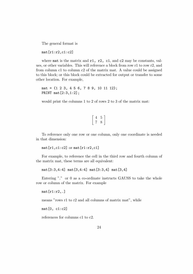
mat = {1 2 3, 4 5 6, 7 8 9, 10 11 12};PRINT mat[2:3,1:2];
would print the columns 1 to 2 of rows 2 to 3 of the matrix mat:
·4 57 8
¸
To reference only one row or one column, only one coordinate is neededin that dimension:
mat[r1,c1:c2] or mat[r1:r2,c1]
For example, to reference the cell in the third row and fourth column ofthe matrix mat, these terms are all equivalent:
mat[3:3,4:4] mat[3,4:4] mat[3:3,4] mat[3,4]
Entering ”.” or 0 as a co-ordinate instructs GAUSS to take the wholerow or column of the matrix. For example
mat[r1:r2,.]
means ”rows r1 to r2 and all columns of matrix mat”, while
mat[0, c1:c2]
references for columns c1 to c2.
24

A whole matrix could then be referred to identically as
mat or mat[.,.]
This particular feature of GAUSS causes a number of unexpected prob-lems, particularly when using loops to access columns or rows in sequence.If your counter drops to zero (or some unspecified values) then you will findthe program operating on all rows or columns instead of just one.For vectors only one co-ordinate is needed. For a column vector, say,
these are all identical
mat[r1:r2,.] mat[r1:r2,0] mat[r1:r2,1] mat[r1:r2]
For scalars there is obviously no need for co-ordinates. However, becausea scalar is a subclass of matrix,
mat[1,1] mat[.,.] mat[1] mat[1,0]
or a number of other variations are acceptable.
This similarity in accessing matrices of zero, one, or two dimensions allowsyou to program loops to access matrices without necessarily knowing thedimensionality of the matrix in advance.A last way to identify a set of rows or columns is to list them sequentially.
For example, to refer to columns 1, 3, and 22 and rows 2 to 4 inclusive of thematrix mat we could use
mat[2:4,1 3 22]
Note that that there are no separating commas in the list ofcolumns; GAUSS treats everything up to the comma as a row reference,everything afterwards as a column reference. If it finds two or more commaswithin square brackets, it treats this as an error.
These different methods can be combined:
mat[1 3:5 9, .]
will select every column on rows 1, 3 to 5, and 9.
25
The order is also important:
mat[1 2 3, .]mat[3 2 1, .]
will give two matrices with the row order reversed in the second one.
6.2.2 Indirect references
Elements of matrices can also be referred to indirectly. Instead of explicitlyusing a constant to indicate a row or column number, a variable can also beused. For example,
PRINT mat[1:5, .];endRow = 5;PRINT mat[1:endRow, .];
are equivalent. This is a key feature in all but the most simple programs,as it avoids having to write out references explicitly. For example, supposethe program is to print out ten lines of a matrix. One solution would be towrite a command to print each line:
PRINT mat[1,.];PRINT mat[2,.];...
This is clearly a tedious process. But one could write a loop to changethe value of a variable i from 1 to 10. Then, only one PRINT statement isneed in the loop:
PRINT mat[i,.];
Even more usefully, this feature will work even if you are unsure howmany lines there are in the matrix. You can set the loop to go as many timesround as there are lines in the matrix. The PRINT statement does not haveto be changed at all.
Similarly, instead of entering explicilty a list of column or row numbers tobe selected, if you enter a vector then GAUSS will use these as the indexes.For example, if rowv is a vector containing (1, 2, 3) then
26

mat[1 2 3, .]; and mat[rowv,.];
are equivalent.
6.2.3 Nested references
Indirect references could be nested. If rowv and colv are a vectors of num-bers, then
mat[rowv[1]:rowv[2], .]
is legal. So is
mat[rowv[r1,c1]:rowv[r2,c2], colv[rowv[r3, c3], rowv[r4,c4]]]
if values have been assigned to r1, c1... and the matrices rowv and colvhave the relevant dimensions. This process can be carried on ad infinitum.
However, one problem with this flexibility in referencing is that GAUSSwill always try to find a solution. For example, to access the first row ofmatrix mat you could use the vector rowv (above), one could use
mat[rowv[1],.]
However, if you omit the index
mat[rowv,.]
then GAUSS will interpret this row vector as a list of rows to be selected,as in the previous section. It will not report an error, as this construct isperfectly acceptable.
27
7 Managing data - SHOW, PRINT, FOR-MAT, NEW, CLEAR, DELETE
These commands are introduced at this point as they are the basic ones formanaging data. DELETE may only be used at the command line, but allthe others can be included in programs.
7.1 SHOW
SHOW displays the name, size and memory location of all global variables andprocedures in memory at any moment. The format is
SHOW varName;SHOW/m varName;
where varName is the variable of interest. The ”wild card” symbol ”*”can be used, so that
SHOW er* ;
will find all references beginning with ”er”. The /m parameter means thatonly matrices are displayed.
7.2 PRINT and FORMAT
PRINT displays the contents of matrices and strings. The format is
PRINT var1 var2 var3... varx ;
which prints the list of variables. How it prints depends on the data. Ifthe data fits on one line (all row vectors, scalars, or strings) then PRINT willdisplay one after the other on the same line. If, however, one of the variablesis a matrix or column vector, then the variable immediately following thematrix will be printed on a new line.
PRINT wraps round when it reaches the end of the line. Each PRINTcommand will start off on a new line. To display without going on to a newline, the PRINT statement must be ended with two semi-colons; this stopsPRINT adding a carriage return to the variable list. For example, consider
28

PRINT ’’Hello’’;PRINT ’’Mum’’; and PRINT ’’Hello’’;;PRINT ’’Mum’’; and PRINT ’’Hello’’ ’’Mum’’;
These display, respectively,
HelloMum HelloMum HelloMum
If strings or string constants (as above) are used, PRINT will recognisethat this is character data. If, however, PRINT is given a matrix name, itmust be informed if this matrix is to be printed as character data. This isdone by prefixing the variable name with the dollar sign $. Hence
a = 1;b = 3;c = ’’Some string data’’;d = ’’char.’’ | ’’matrix’’; PRINT a b c $d;
prints everything correctly. Matrices composed entirely of character dataare shown in the same way; however, mixed matrices needs special com-mands, PRINTFM and PRINTFMT, of which more later.
Remark 1 Once GAUSS comes across a $ sign indicating character data,it prints all the rest of that line as text. Thus
PRINT a $c b;
would lead to ’b’ being treated as if it were text. To get round this, ’b’must be printed in a separate statement, perhaps using the double-colon:
PRINT a $c;;PRINT b;
PRINT style is controlled by the FORMAT commands, which sets theway matrices (but not strings) are printed. There are options to print num-bers and character data with varying field widths, decimal expansion, justi-fication, spacing and punctuation. These are covered in the manual and areall similar in form to:
29
FORMAT /RD 6, 0;
where, in this case, we have numbers right-justified (/RD), separated byspaces (/RDC would do commas), with 6 spaces left for writing the numberand 0 decimal places. If the number is too large to fit into the space, thenthe field will be expanded but for that number only - not the whole matrix.Strings are given as much space as they need, but no spaces are insertedbetween them (see the ”HelloMum” example, above).The print styles set by FORMAT operate from the time they are set until
the next FORMAT command is received.
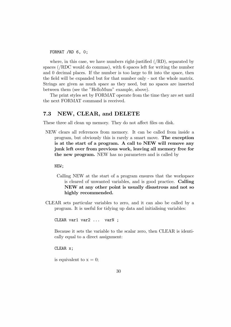
7.3 NEW, CLEAR, and DELETE
These three all clean up memory. They do not affect files on disk.
NEW clears all references from memory. It can be called from inside aprogram, but obviously this is rarely a smart move. The exceptionis at the start of a program. A call to NEW will remove anyjunk left over from previous work, leaving all memory free forthe new program. NEW has no parameters and is called by
NEW;
Calling NEW at the start of a program ensures that the workspaceis cleared of unwanted variables, and is good practice. CallingNEW at any other point is usually disastrous and not sohighly recommended.
CLEAR sets particular variables to zero, and it can also be called by aprogram. It is useful for tidying up data and initialising variables:
CLEAR var1 var2 ... varN ;
Because it sets the variable to the scalar zero, then CLEAR is identi-cally equal to a direct assignment:
CLEAR x;
is equivalent to x = 0;
30
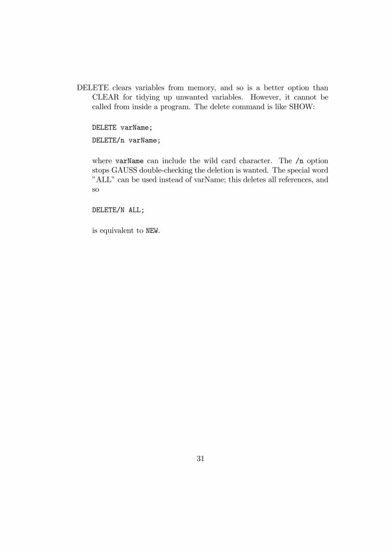
DELETE clears variables from memory, and so is a better option thanCLEAR for tidying up unwanted variables. However, it cannot becalled from inside a program. The delete command is like SHOW:
DELETE varName;
DELETE/n varName;
where varName can include the wild card character. The /n optionstops GAUSS double-checking the deletion is wanted. The special word”ALL” can be used instead of varName; this deletes all references, andso
DELETE/N ALL;
is equivalent to NEW.
31

8 GAUSS procedures• The library functions in GAUSS work like library routines in otherpackages - a procedure is called with some parameters, something hap-pens, and a result may be returned.
• The parameters may be constants or variables; any returned valuesmust be placed in variables. There may be any number of input andoutput parameters, including none.
• The general format in
{outVar1, ...outVarN} = ProcName (inVar1, ... inVarN);
The inVar parameters are giving information to the procedure; theoutVar variables are collecting information from the procedure. Theinput parameters will be unaffected by the action of the procedure(unless, of course, they also feature in the output list). The outVarparameters will be affected, and so obviously constants can not beused:
{outVar1, ’’eric’’} = ThisProc (inVar1, inVar2);
is incorrect.
Note that we have curly brackets {} to group variables together forthe purposes of collecting results, but that we have round brackets ()to delineate the input parameters. The former is GAUSS’s usual way ofgrouping things together, the latter is a near-universal programming syntax.They’re mixed in together just to keep you on your toes.
If there is one or no parameter, then the form can be simplified:
{outVar1, ... outVarx} = ProcName (inVar); one input parameter{outVar1, ... outVarx} = ProcName; no input parameterProcName (inVar1, ... inVarx); no returned resultoutVar = ProcName (inVar1, ...inVarx); one result returned
32

For example, the procedure DELIF requires two input parameters (a ma-trix and a column vector), and returns one output, a matrix:
outMat = DELIF (inMat, colVec);
The procedure EIGCG requires two input parameters and two outputparameters
{eigsReal, eigsImag} = EIGCG(matReal, matImag);
The procedure SORT needs four input parameters but returns no result:
SORT (inFile, outFile, keyName, keyType);
If the program is not concerned with the results from procedure then thefunction CALL tells GAUSS to throw away any returns. This can save timeand memory in some cases. For example, the quickest way to find the deter-minant of a large matrix is through a Cholesky decomposition. Running theprocedure CHOL sets a global variable which can be read by the procedureDETL to give the matrix’s determinant. However, the actual result of thedecomposition is not wanted, only a side effect. So, to find the determinantof ”mat” most quickly use
CALL CHOL(mat);determ = DETL;
As input and returned parameters are both lists, you can pass the wholelist of returned parameters to a new function, along with any other param-eters that are necessary. This means that you do not need to have anyintermediate variables to store the results from one procedure before passingthem to another, and it will make your code shorter. However, it will notnecessarily make it more readable, and you can run into maintenance prob-lems - if you change the list of parameters for one procedure you need tochange it for the other as well.
Remark 2 For all procedures, it is the programmer’s responsibility to ensurethat the right sort of data is used. If a procedure is expecting a scalar as aparameter and you pass it a row vector, for example, this will not be flaggedas an error when GAUSS checks the program syntax. It may or may not
33

cause the procedure to crash but this will not be apparent until the programis running. All GAUSS will check is that the correct number of parametersis being passed back and forth.
34

9 Matrix algebraAlgebra involving matrices translates almost directly from the page intoGAUSS. At bottom, most mathematical statements can be directly tran-scribed, with some small changes.
9.1 The basic operators
GAUSS has eight mathematical operators and six relational ones.The mathematical ones are
+ Addition- Subtraction* Multiplication/ Division
’ Transposition% Modulo division! Factorial
^ Exponentiation
The relational operators are:
== EQ equals/= NE does not equal> GT greater than< LT less than
>= GE greater than/equals<= LE less than/equals
Either the symbols or the two-letter acronyms may be used.
Warning
35
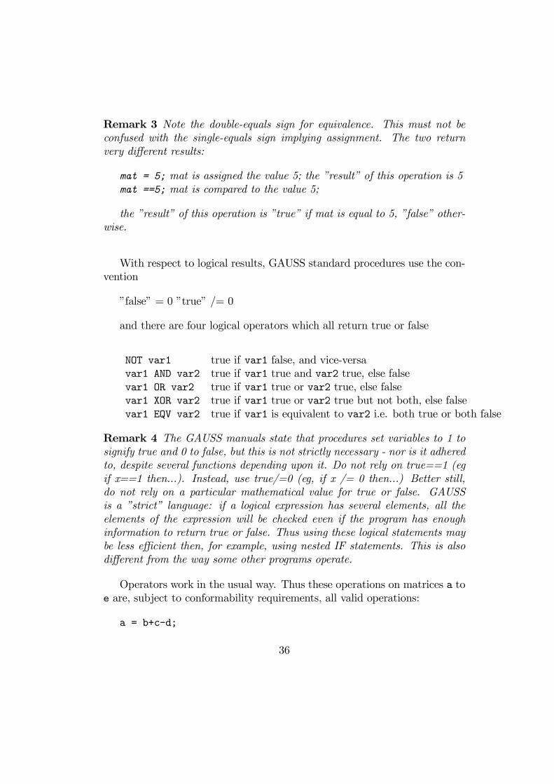
Remark 3 Note the double-equals sign for equivalence. This must not beconfused with the single-equals sign implying assignment. The two returnvery different results:
mat = 5; mat is assigned the value 5; the ”result” of this operation is 5mat ==5; mat is compared to the value 5;
the ”result” of this operation is ”true” if mat is equal to 5, ”false” other-wise.
With respect to logical results, GAUSS standard procedures use the con-vention
”false” = 0 ”true” /= 0
and there are four logical operators which all return true or false
NOT var1 true if var1 false, and vice-versavar1 AND var2 true if var1 true and var2 true, else falsevar1 OR var2 true if var1 true or var2 true, else falsevar1 XOR var2 true if var1 true or var2 true but not both, else falsevar1 EQV var2 true if var1 is equivalent to var2 i.e. both true or both false
Remark 4 The GAUSS manuals state that procedures set variables to 1 tosignify true and 0 to false, but this is not strictly necessary - nor is it adheredto, despite several functions depending upon it. Do not rely on true==1 (egif x==1 then...). Instead, use true/=0 (eg, if x /= 0 then...) Better still,do not rely on a particular mathematical value for true or false. GAUSSis a ”strict” language: if a logical expression has several elements, all theelements of the expression will be checked even if the program has enoughinformation to return true or false. Thus using these logical statements maybe less efficient then, for example, using nested IF statements. This is alsodifferent from the way some other programs operate.
Operators work in the usual way. Thus these operations on matrices a toe are, subject to conformability requirements, all valid operations:
a = b+c-d;
36
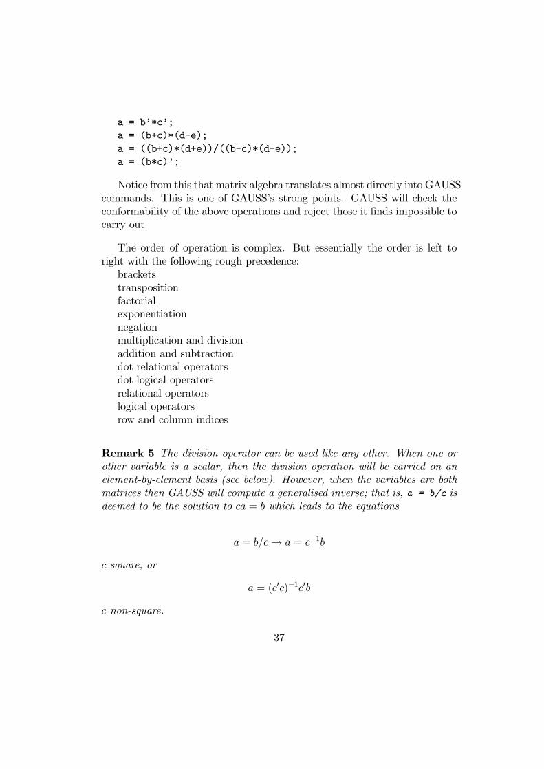
a = b’*c’;a = (b+c)*(d-e);a = ((b+c)*(d+e))/((b-c)*(d-e));a = (b*c)’;
Notice from this that matrix algebra translates almost directly into GAUSScommands. This is one of GAUSS’s strong points. GAUSS will check theconformability of the above operations and reject those it finds impossible tocarry out.
The order of operation is complex. But essentially the order is left toright with the following rough precedence:bracketstranspositionfactorialexponentiationnegationmultiplication and divisionaddition and subtractiondot relational operatorsdot logical operatorsrelational operatorslogical operatorsrow and column indices
Remark 5 The division operator can be used like any other. When one orother variable is a scalar, then the division operation will be carried on anelement-by-element basis (see below). However, when the variables are bothmatrices then GAUSS will compute a generalised inverse; that is, a = b/c isdeemed to be the solution to ca = b which leads to the equations
a = b/c→ a = c−1b
c square, or
a = (c0c)−1c0b
c non-square.
37

Therefore, if two matrices are divided, then it may be preferable to dothe inverse explicitly rather than leave the calculation to GAUSS. Divisionis a common source of unnoticed errors, because GAUSS will try as hard aspossible to find an appropriate inverse.
9.1.1 Concatenation
There are two concatenation operators:
~ horizontal concatenation| vertical concatenation
These add one matrix to the right or bottom of another. Obviously, therelevant rows and columns must match. Consider the following operationson two matrices, a and b, with ra and rb rows and ca and cb columns, andthe result placed in the matrix c:
dimensions of a dimensions of b operation dimensions of c conditionra× ca rb× cb c = a ~b ra× (ca+ cb) ra = rbra× ca rb× cb c = a | b (ra+ rb)× ca ca = cbParts of matrices may be used, and results may be assigned to matrices
or to parts:
a = b*c;a = b[r1:r2,c1]*c[r3, c2:c3];a[r1, c1:c2] = b[r1,.]*c;
subject to, in the last case, the recipient area being of the correct size.These operations are available on all variables, but obviously ”a=b*c” is
nonsensical when b and c are strings or character matrices. However, therelational operators may be used; and there is one useful numerical operator- addition:
a = b $+ c;
This appends c to b. Note that the operator needs the string signifier ”$”to inform GAUSS to do a string concatenation rather than a numericaladdition. If you omit the $ GAUSS will carry out a normal addition.For example,
38

b = ’’hello’’;c = ’’mum’’;a = b $+ ’’ ’’ $+ c;PRINT $a;
will lead to ”hello mum” being printed.With character matrices, the rules for the conformability of matrices and
the application of the operator are the same as for mathematical operators.Note that, in contrast to the matrix concatenation operators, the overallmatrix remains the same size (strings grow) but each of the elements in thematrix will be changed. Thus if a is an r × c matrix of file names,
a = a $+ ’’.RES’’;
will add the extension ”.RES” to all the names in the matrix (subject tothe eight-character limit) but a will still be an (r × c) matrix. If any of thecells then have more than eight characters, the extra ones are cut off.String concatenation applied to strings and string arrays will cause these
to grow.Strings and character matrices may be compared using the relational
operators. The string signifier $ is not always necessary, but it makes theprogram more readable and may avoid unexpected results.In the eight bytes of data used for each matrix cell, characters and num-
bers are stored in different ways. GAUSS uses the $ symbol to signify thebyte order, but otherwise makes no distinction between characters and num-bers. So if you mix data types, omit a $ sign or put one in where it shouldn’tbe, GAUSS will not complain but the result will be gibberish.
9.1.2 Conformability and the ”dot” operators
GAUSS generally operates in an expected way. If a scalar operand is appliedto a matrix, then the operation will be applied to every element of the matrix.If two matrices are involved, the usual conformability rules apply:
39

Operation Dimensions of b Dimensions of c Dimensions of aa = b * c; scalar 4× 2 4× 2a = b * c 3× 2 4× 2 illegala = b * c’; 3× 2 4× 2 3× 4a = b + c; scalar 4× 2 4× 2a = b - c; 3× 2 4× 2 illegala = b - c; 3× 2 3× 2 3× 2and so on.However, GAUSS allows most of the mathematical and logical operators
to be prefixed by a dot:
a = b.>c; a = (b+c).*d’; a = b.==c;
This tells the machine that operations are to be carried out on an ”elementby element” basis (or ExE, as the manual so succinctly puts it). This meansthat the operands are essentially broken down into the smallest conformableelements and then the scalar operators are applied. How this works in prac-tice depends on the matrices.To give an example, suppose that mat1 is a (5× 4) matrix. Then the
following results occur for multiplication:
Operation dimensions of mat2 Resultmat1 * mat2 scalar 5× 4; mat2 times each element of mat1mat1 .* mat2 (5× 4) 5× 4; mat1[i,j] * mat2[i,j] for all i, j (mat1¯mat2)mat1 .* mat2 (5× 1) 5× 4; mat1[j,i] is multiplied by mat2[j] for all i,jmat1 .* mat2 (1× 4) 5× 4; mat1[j,i] is multiplied by mat2[i] for all i,jmat1 .* mat2 anything else illegal
Similarly for the other numerical operators:Operation dimensions of mat2 Resultmat1 ./ mat2 5× 4 5× 4; mat1[i,j] / mat2[i,j] for all i, jmat1 .% mat2 1× 4 5× 4; modulus mat1[i,j] / mat2[j] for all i, jmat1 .*. mat2 5× 4 25× 16; mat1[i, j] * mat2 for all i,j (mat1⊗mat2)
Remark 6 The dot operators do not work consistently across all operands.In particular, for addition and subtraction no dot is needed.
40

Examplenew;x = {2 5,0.9 11};y = {.5 .2,3 4};
z = y .*. x;v = x *~ y;
x =
·2 50.9 11
¸
y =
·0.5 0.23 4
¸
v =
·x11 × y11 x11 × y12 x12 × y11 x12 × y12x21 × y21 x21 × y22 x22 × y21 x22 × y22
¸
v =
·1 0.4 2.5 12.7 3.6 33 44
¸9.1.3 Relational operators and dot operators
For the relational operators, the results are slightly different. These operatorsreturn a scalar 0 or 1 in normal circumstances; for example, compare twoconformable matrices:
mat1 /= mat2;
mat1 GT mat2;
The first returns ”true” if every element of mat1 is not equal to everycorresponding element of mat2; the second returns ”true” if every element ofmat1 is greater than every corresponding element of mat2. If either variableis a scalar than the result will reflect whether every element of the matrixvariable is not equal to, or greater than, the scalar. These are all scalarresults.
41
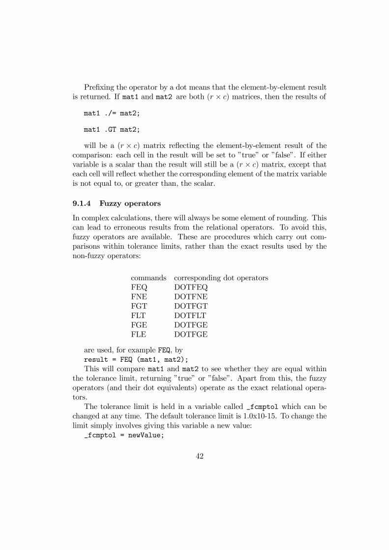
Prefixing the operator by a dot means that the element-by-element resultis returned. If mat1 and mat2 are both (r × c) matrices, then the results ofmat1 ./= mat2;
mat1 .GT mat2;
will be a (r × c) matrix reflecting the element-by-element result of thecomparison: each cell in the result will be set to ”true” or ”false”. If eithervariable is a scalar than the result will still be a (r × c) matrix, except thateach cell will reflect whether the corresponding element of the matrix variableis not equal to, or greater than, the scalar.
9.1.4 Fuzzy operators
In complex calculations, there will always be some element of rounding. Thiscan lead to erroneous results from the relational operators. To avoid this,fuzzy operators are available. These are procedures which carry out com-parisons within tolerance limits, rather than the exact results used by thenon-fuzzy operators:
commands corresponding dot operatorsFEQ DOTFEQFNE DOTFNEFGT DOTFGTFLT DOTFLTFGE DOTFGEFLE DOTFGE
are used, for example FEQ, byresult = FEQ (mat1, mat2);This will compare mat1 and mat2 to see whether they are equal within
the tolerance limit, returning ”true” or ”false”. Apart from this, the fuzzyoperators (and their dot equivalents) operate as the exact relational opera-tors.The tolerance limit is held in a variable called _fcmptol which can be
changed at any time. The default tolerance limit is 1.0x10⁻¹⁵. To change thelimit simply involves giving this variable a new value:_fcmptol = newValue;
42

10 Set operationsColumn vectors can be treated like sets for some purposes. GAUSS providesthree standard procedures for set operation:
unVec = UNION (vec1, vec2, flag);intVec = INTRSECT (vec1, vec2, flag);difVec = SETDIF (vec1, vec2, flag);
where unVec, intVec, and difVec are the results of union, intersection,and difference operations on the two column vectors vec1 and vec2. Thescalar flag is used to indicate whether the data is character or numeric: 1 fornumeric data, 0 for character. The difference operator returns the elementsof vec1 not in vec2, but not the elements of vec2 not in vec1.These commands will only work on column vectors (and obviously scalars).
The two vectors can be of different sizes. A related command to the set op-erators is
unVec = UNIQUE (vec, flag);
which returns the column vector vec with all its duplicate elements re-moved and the remaining elements sorted into ascending order.
11 Special matrix operationsGAUSS provides methods to create andmanipulate a number of useful matrixforms. The commonest are covered in this section. A fuller description is tobe found in the GAUSS Command Reference.
11.1 Some useful matrix types
Firstly, three useful matrix creating operations:
identMat = EYE (iSize);onesMat = ONES (onesRows, onesCols);zerosMat = ZEROS (zeroRows, zeroCols);
These create, respectively: an identity matrix of size iSize; a matrix ofones of size onesRows by onesCols; and a matrix of zeroes of size zeroRowsby zeroCols.
43

11.2 Special operations
A number of common mathematical operations have been coded in GAUSS.These are simple to use to use and more efficient then building them up fromscratch. They are
invMat = INV (mat);invPDMat = INVPD (mat);momMat = MOMENT (mat, missFlag);determ = DET (mat);determ = DETL;matRank = RANK (mat);
The first two of these invert matrices. The matrices must be squareand non-singular. INVPD and INV are almost identical except that the inputmatrix for INVPD must be symmetric and positive definite, such as a momentmatrix. INV will work on any square invertible matrix; however, if the matrixis symmetric, then INVPD will work almost twice as fast because it uses thesymmetry to avoid calculation. Of course, if a non-symmetric matrix is givento INVPD, then it will produce the wrong result because it will not check forsymmetry.GAUSS determines whether a matrix is non-singular or not using another
tolerance variable. However, even if it decides that a matrix is invertible, theINV procedure may fail due to near-singularity. This is most likely to bea problem on large matrices with a high degree of multicollinearity. TheGAUSS manual suggests a simple way to test for singularity to machineprecision.The MOMENT function calculates the cross-product matrix from mat; that
is, mat’*mat. For anything other than small matrices, MOMENT(x, flag) ismuch quicker than using x0x explicitly as GAUSS uses the symmetry of theresult to avoid unnecessary operations. The missFlag instructs GAUSS whatto do about missing values - whether to ignore them (missFlag=0) or excisethem (missFlag=1 or 2).DET and DETL compute the determinants of matrices. DET will return the
determinant of mat. DETL, however, uses the last determinant created byone of the standard functions; for example, INV, DET itself, decompositionfunctions all create determinants along the way. DETL simply reads this value.Thus DETL can avoid repeating calculations. The obvious drawback is that itis easy to lose track of the last matrix passed to the decomposition routines,
44

and so determinants should be read as soon as possible after the relevantdecomposition function has been called. See the Command Reference fordetails of which procedures create the DETL variable.RANK calculates the rank of mat.
11.3 Manipulating matrices
There are a number of functions which perform useful little operations onmatrices. Commonly-used ones are:
vec = DIAG (mat);mat = DIAGRV (vec);newMat = DELIF (oldMat, flagVec);newMat = SELIF (oldMat, flagVec);newMat = RESHAPE (oldMat, newRows, newCols);nRows = ROWS (mat);nCols = COLS (mat);maxVec = MAXC (mat);minVec = MINC (mat);sumVec = SUMC (mat);
DIAG and DIAGRV abstract and insert, respectively, a column vector fromor into the diagonal of a matrix.DELIF and SELIF allow certain rows and columns to be deleted from the
matrix oldMat. The column vector flagVec has the same number of rowsas oldMat and contains a series of ones and zeros. DELIF will delete all therows from the matrix for which there is a corresponding one in flagVec, whileSELIF will select all those rows and throw away the rest. Therefore DELIFand SELIF will, between themselves, cover the whole matrix.DELIF and SELIFmust have only ones and zeros in flagVec for the function
to work properly. This is something to consider as the vector flagVec is oftencreated as a result of some logical operation. For example, to delete all therows from matrix mat1 whose first two columns are negative would involve
flags = (mat1[1,.] .< 0) .AND (mat1[2,.] .< 0);mat2 = DELIF (mat1, flags);
45

This particular example should work on most systems, as the logical op-erator AND only returns 1 or 0. But because true is really non-zero (not 1)some operations could lead to unexpected results.DELIF and SELIF also use a lot of memory to run.ROWS and COLS return the number of rows and columns in the matrix of
interest.MAXC, MINC, and SUMC produce information on the columns in a matrix.
MAXC creates a vector with the number of elements equal to the number ofcolumns in the matrix. The elements in the vector are the maximum numbersin the corresponding columns of the matrix. MINC does the same for minimumvalues, while SUMC sums all the elements in the column. However, note thatall these functions return column vectors. So, to concatenate onto the bottomof a matrix the sum of elements in each column would require an additionaltransposition:
sums = SUMC(mat1);mat1 = mat1 | sums’;
On the other hand, because these functions work on columns, then callingthe functions again on the column vectors produced by the first call allowsfor matrix-wide numbers to be calculated:
maxMat=MAXC(MAXC(mat1));minMat=MINC(MINC(mat1));sumMat=SUMC(SUMC(mat1));
will return the largest value in mat1, the smallest value, and the totalsum of the elements.
46

12 Examplesnew;x = {2 5,0.9 11};y = {0.5 0.2,3 4};z = y.*.x;v = x.^y;x*~y;print z;print v;
new;let x[2,2] = 1 0 2 0;let y[2,2] = 1 5 0 0;
z = .NOT x;print z;z = x.and y;print z;
z = ( ( .NOT x) .XOR y ) .OR Y;print z;
new;let x[2,2] = 1 0 2 0;let y[2,2] = 1 5 4 2;z = x > y;print z;z = x <= y;print z;z = x == y;print z;z = x .== y;print z;z = x ./= y;print z;z = (x ./=y) .AND (x.==y);
47

print z;
48

new;x = seqa(1,1,4);y = x’*ones(10,4);indx = {1 3 4};z = y[.,indx];print z;
new;y = rndn(100,4);ex = y[.,2] .> 0.5;suby = selif(y,ex);print suby;ex2 = abs(y[.,1]) .< 0.33 .AND y[.,2] .> 0.66;suby2 = selif(y,ex);print suby2;ex = y[.,1] .< 0.33;y = delif(y,ex);
49

13 Manipulating Matrices 2• Y = Cumsumc(A); Computes the cumulative sums of the columns of amatrix.
• Z = Complex(X,Y); Converts a pair of real matrices to a complex ma-trix (X (N ×K) real matrix, the real elements of Z.
• Y = Imag(A); Returns the imaginary part of a matrix.• Y = Maxindc(A); Returns a column vector containing the index (i.e.,row number) of the maximum element in each column in a matrix.
• Y = Minindc(A); Returns a column vector containing the index (i.e.,row number) of the smallest element in each column in a matrix.
• Y = Reshape(X,r,c); reshapes a matrix.Input
X (N ×K) matrix.r scalar, new row dimension.
c scalar, new column dimension.
Output
Y (R × C) matrix created from the elements of X.
The first c elements are put into the first row of Y, the second c elementsin the second row, and so on.
If there are more elements in X than in Y, the remaining are discarded.If there are not enough elements in X to fill in Y it goes back to thefirst elements of X and starts getting additional elements from there.
Example
new;
x = rndn(7*100,1); /* (700 * 1) vector */
y = reshape(x,100,7);
/*reshaping in a (100 * 7) matrix */
call printfmt(x[8:14],1);
50

print;
call printfmt(y[2,.],1);
Example
new;
let Let A[3,3] = 1 2 3 4 5 6 7 8 9 ;
B = reshape(A,2,4);
print ’’reshape(A,2,4) =’’;
call printfmt(B,1);
C = reshape(A,6,4);
print ’’reshape(A,6,4) =’’;
call printfmt(C,1);
• Y = Rev(A) Inversion of rows• Y = Trimr(X,A,B) Trimming of the first A rows and the last B rows.• Y = Lag1(X);Lags a matrix by one time period for time series analysis.Input
X (N ×K) matrix.Output
Y (N ×K) matrix. First observations of y are missing.• Y = Lagn(X,M); Lags or leads a matrix a specified number of timeperiods for time series analysis.
Input
X (N ×K) matrix.M number of time periods
Z (N ×K) matrix.Output
Y (N ×K) matrix. If M>0, lagn lags X back M time periods, so thefirst M observations of Y are missing. If M<0, lagn lags X forward Mtime periods, so the last M observations of Y are missing.
51

Example
X (10× 2)
Z = Lag1(X);
Z =
· ·x11 x12...
...x91 x92
Z = Lagn(X,2);
Z =
· ·· ·x11 x12...
...x81 x82
Example
new;
T = 10;
x = seqa(1,1,T);
xt = lagn(x,-1);
xt_1 = lag1(x);
print xt;
print xt_1;
xt = trimr(xt,0,1);
xt_1 = trimr(xt_1,1,0);
print;
print xt_1;
print xt;
52

• Y = vec(X); Creates a column vector by appending the columns/rowsof a matrix to each other.
Input
X (N ×K) matrix.Output
Y (N ×K)× 1 vector, the columns of x appended to each other.• Y = Seqa(S,H,N) creates an additive sequence
Yj = S + (N − 1)H
• Y = Seqm(S,H,N) creates a multiplicative sequence
Yj = SHN−1
53

14 Mathematical Functions• Y = Abs(X) absolute value or module• Y = Cos(X) cosine• Y = Sin(X) sine• Y = Exp(x) exponential• Y = Gamma(X) Γ (x) =
R∞0tx−1e−tdt
• Y = Ln(X) natural log• Y = Sqrt(X) square root• Y = Tan(X) tangent• P = Chol(A) Cholesky’s Decomposition of a symmetric, positive defi-nite matrix A = P 0P , P upper triangular
• {Va,Ve} = Eighv(M) Eigenvalues and Eigenvectors of complex hermi-tian or real symmetric matrix
• {Va,Ve} = Eigv(M) Eigenvalues and Eigenvectors of a general matrix• Va = Eigh(M) Eigenvalues of complex hermitian or real symmetricmatrix
• Va = Eig(M) Eigenvalues of a general matrix• Y = Gradp(&f,X) Jacobian of function F in X• Y = Hessp(&f,X) Hessian of function F in X• B = Inv(A) Inverse of A• B = Invpd(A) Inverse of a positive definite matrix• B = Pinv(A) Generalised Inverse (Moore-Penrose)• C = Polychar(A) Characteristic Polynomial of A• C = Polyroot(A) Roots of a polynomial
54

ExampleDecomposition of a symmetric p.d. matrix X corresponds to the command
CHOL, i.e. Cholesky Decomposition:
X = Q0Q
where Q is an upper triangular matrix.Let
P = Q0
Suppose we want to simulate random vectors from a multivariate normalN(mu, Sigma).
N(mu, Sigma) = mu+ P ∗N(0, 1)
new;rndseed 123;let mu = 10 12 2;let Sigma[3,3] =2.2 0.5 0.00.5 1.2 -.60.0 -.6 1.8;P = chol(Sigma)’;print ’’P = ’’ P;print ’’P*P’ = ’’ P*P’;/* simulation of a random vector u~N(mu,Sigma) */u = mu + P*rndn(3,1);print ’’u = ’’ u;u = mu + P*rndn(3,1000); /* simulation of 1000 r.v. */u = u’;smean = meanc(u);scov = vcx(u);print ’’Sample mean = ’’ smean;print ’’Sample covariance matrix = ’’ scov;cumsumc(u)./seqa(1,1,1000);
55

15 Statistical Functions• Y = Cdfn(X) R x−∞ φ (s) ds
• Y = Cdfnc(X) 1− R x−∞ φ (s) ds
• Y = Cdfchic(X,n) Computes the complement of the cdf of the chi-square distribution.
Y is the integral from x to 8of the chi-square distribution with n degreesof freedom.
• Y = Cdftc(X,N) Computes the complement of the cdf of the Studentst distribution.
• C = Corrx(X) Correlation matrix of matrix X• M = Meanc(X) Means of columns• S = Stdc(X) Standard deviation of matrix X’s columns• V = Vcx(X) Variance-covariance matrix X• N = Rndn(K,L) (K × L) Matrix of standard normal pseudo-randomnumbers
• U = Rndu(K,L) (K × L) Matrix of uniform pseudo-random numbers
• Rndseed seednumber
56

Example
rndseed 5390;p =100;q = 10;x = rndn(p,q);mu = meanc(x);st = stdc(x);vc = vcx(x);print ’’sample mean ’’ mu;print ’’sample variance’’ st.^2;print ’’variance-covariance matrix’’;print;vc;
Examplenew;rndseed 4572;u = rndu(1000,1);x = 10 + 2*u;y = x.*lag1(x).*lagn(x,2).*lagn(x,3);y = trimr(y,3,0);/* Correlation coefficient
ρ =1N
PNt=1 (xt − x) (yt − y)h
1N
PNt=1 (xt − x)2
i1/2 h1N
PNt=1 (yt − y)2
i1/2*/
x = trimr(x,3,0);yc = y - meanc(y);xc = x - meanc(x);covxy = meanc(xc.* yc);sigmax = sqrt(meanc(xc .* xc));sigmay = sqrt(meanc(yc.*yc));corrxy = covxy ./ (sigmax*sigmay);print corrxy;corrx(y~x);
57

16 Strings• ^ interprets the following name as a variable• Y = Chrs(X) converts a matrix of ASCII codes to character string• Y = Ftocv(X,Field,Prec) character representation of numbers in (N ×K)matrix. It converts a matrix containing floating point numbers into amatrix containing the decimal character representation of each element.
Input
X (N ×K) matrix containing numeric data to be converted.Field scalar, minimum field width.
Prec scalar, the numbers created will have prec places after the decimalpoint.
Output
Y (N ×K) matrix containing the decimal character equivalent of thecorresponding elements in X in the format defined by field and prec.
• Y = Getf(filename,mode) loads ASCII or Binary file into string.Input
filename string, any valid file name.
mode scalar 1 or 0 which determines if the file is to be loaded in ASCIImode (0) or binary mode (1).
Output
Y string containing the file.
• Y = Stof(X) converts string to floating pointInput
X (N ×K) matrix containing numeric data to be converted.Output
Y matrix, the floating point equivalents of the ASCII numbers in x.
Examplen=5;print chrs(ones(n,1)*42);
58

17 Printing• Printfmt(X,mask);Input
X (N ×K) matrix which is to be printed.mask scalar, 1 if X is numeric or 0 if X is character or (1×K) vector of1’s and 0’s.
The corresponding column of x will be printed as numeric where mask= 1 and as character where mask = 0.
• Y = Ftos(X,Fmat,Field,Prec) converts a scalar into a string con-taining the decimal character representation of that number.
Input
X scalar
Fmat the format stirng to control the conversion
Field scalar or (2× 1) vector, the minimum field width
Prec scalar or (2× 1) vector, the numbers of places following thedecimal point.
Output
Y string containing the decimal character equivalent of X in formatspecified.
59
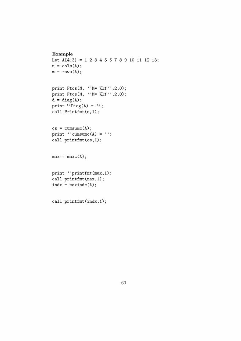
ExampleLet A[4,3] = 1 2 3 4 5 6 7 8 9 10 11 12 13;n = cols(A);m = rows(A);
print Ftos(N, ’’M= %lf’’,2,0);print Ftos(M, ’’M= %lf’’,2,0);d = diag(A);print ’’Diag(A) = ’’;call Printfmt(s,1);
cs = cumsumc(A);print ’’cumsumc(A) = ’’;call printfmt(cs,1);
max = maxc(A);
print ’’printfmt(max,1);call printfmt(max,1);indx = maxindc(A);
call printfmt(indx,1);
60

ExampleLet x = 125.34985027;let y = 3.21;let z = 5;
field = 1;prec = 0;fmat = ’’%*.*lf’’;ftos(z,fmat,field,prec);
field = 7;prec = 2;fmat = ’’%*.*lf seconds’’;ftos(x,fmat,field,prec);ftos(y,fmat,field,prec);
Example
• new;let Let A[4,3] = 1 2 3 4 5 6 7 8 9 10 11 12 13;;
v = vec(A);
vr =vecr(A) /* vecr(A) = vec(A’) */
print ’’vec(A) vecr(A)’’;
call printfmt(v~vr,1);
B = trimr(A,0,2);
print ’’trimr(A,0,2) = ’’;
call printfmt(B,1);
61

18 Missing ValuesA missing value is a special floating point encoding which the numeric pro-cessor considers a NaN (Not a Number).
• Y = MISS(X,V) elements in X (N ×K) that are equal to the corre-sponding elements in V, (L×M) matrix E × E conformable with X,will be replaced with the GAUSS missing value code.
• Y = MISSRV(X,V) elements in X (N ×K) that are equal to the GAUSSmissing value code will be replaced with the corresponding element ofV (L×M) matrix E ×E conformable with X.
• Y = MISSEX(X,E) converts numeric values in X (N ×K) to the missingvalue code according to the values given in a logical expression (E is a(N ×K) logical matrix).
• M = ISMISS(X) Returns 1 if its matrix argument ((N ×K) matrix)contains any missing values, otherwise returns a 0.
• M = SCALMISS(X) Tests to see if its argument is a scalar missing value.X (N ×K) matrix. The ISMISS function will test each element of thematrix and return 1 if it encounters any missing values.
Examplelet A[3,3] = 1 2 . 4 5 6 7 . 9;scalmiss(a);scalmiss(a[1,3]);
• y = PACKR(X) Deletes the rows of the matrix that contain any missingvalues. X (N ×K) matrix.
• ENABLE; Enables the invalid operation interrupt of the numeric proces-sor. This affects the way missing values are handled in most calcula-tions. When ENABLE is in effect, missing values will not be allowedin most calculations. The default is to have the program crash whenmissing values are encountered or when any operation sets the numericprocessor’s invalid operation exception. If ENABLE is on these oper-ation will cause the program to terminate with ”Invalid floating pointoperation” error message.
62

• DISABLE; It is the opposite of ENABLE. If DISABLE is on these op-erations will return a NaN, and the program will continue.
63

Example
new;msym .;/* The command MSYM changes the character for missing values */
machineEPSILON = machepsilon;
print ’’the smallest number such that 1+ eps > 1’’;print machineEPSILON;
Missingvalue = miss(0,0);print ftos(MissingValue, ’’missing value : %*.*s’’,5,1);print ftos(MissingValue, ’’missing value : %*.*lf’’,5,1);
msym ’’NA’’;print ftos(MissingValue, ’’missing value : %*.*s’’,5,1);
msym -9999.99;print ftos(MissingValue, ’’missing value : %*.*s’’,5,1);print;
let A[3,3] = 1 2 . 4 5 6 7 . 9;print ’’A =’’ A;B = missrv(A,0);print ’’B = ’’ B;C = miss(A,0);print ’’C = ’’ C;D = miss(a,0);print ’’D = ’’ D;
64

19 Exercises1. Generate two random vectors (10× 1), compare them E×E and returna vector of boolean variables.
2. Compare two matrices (generated randomly) and print to screen a mes-sage like ”true” and ”false”.
3. Generate a (10× 10) random matrix (using rndn) extract the rows thathave the first element, i.e. the first column, greater than zero.
4. Generate a (10× 10) random matrix (using rndu) and extract only theelements greater than 0.5, i.e. the output is a new matrix that haszeros in place of the elements less or equal to 0.5.
5. Create a (3× 3) matrix of Gaussian pseudo-random numbers. Use arelational operator to set elements of the matrix that are less than zeroto zero.
6. Create a second (3× 3) matrix of Gaussian pseudo-random numbers.Generate a third matrix that equals the element-by-element productsof the two matrices, conditional on the products being less than zero.All other elements of the third matrix should equal zero.
7. Create two (100× 100) matrices of Uniform pseudo-random numbers.Generate a third matrix with elements equal to the sum of the firsttwo matrices, given that each of the two elements in the sum is greaterthan 0.5. Elements of the third matrix are zero if this condition is notmet. Use sumc to see whether your results roughly match the expectedresults (Hint: First turn the third matrix into ones and zeros).
8. Create a 10 3 matrix of pseudo-random numbers. Generate a columnvector of the means of the columns of the pseudo-randommatrix. Don’tuse meanc for this.
9. Create a column vector containing a sequence of numbers using seqa.Call it s. Create a square matrix of ones with the same number of rowsand columns as rows in the sequence. Call it X. Notice the differencesbetween s.*X and X.*s’. The first element-by-element multiplicationcauses GAUSS to sweep vertically across X. The second causes GAUSSto sweep horizontally, down X.
65

10. Create a string with eight or less characters. Now create a string arraywhere each element of the array is equal to your initial string. Use theones matrix and a multiplication operator to do this, converting themultiplication result to a string array.
11. Create a string array containing VAR1,VAR2,...
12. Create a (5× 5) string array where elements in rows 2 and 3 andcolumns 2 and 3 are set to the letter B and the remaining elementsset to the letter A.
13. Create a (5× 5) Create a 5 5 matrix of missing values. First createa numeric matrix. Convert the numeric matrix to one with missingvalue.
66

20 Flow of controlUp to now all the code used in the examples and exercises has been presentedin a step-by-step way:
instruction1;instruction2;instruction3;...
Both the loop and the conditional branch involve changes in the flowof control of the program: the sequence of instructions that the programexecutes, and the order in which they are executed, is being controlled byother instructions in the program. There are two other ways in which thesequence of instructions can be altered: by the suspension (temporary orpermanent) of execution; and by procedure calls.
GAUSS also provides the ability for unconditional branching (GOTO,BREAK, CONTINUE) and open subroutines (GOSUB).
20.1 Conditional branching: IF
The syntax of the full IF statement is:
IF condition1;doSomething1;ELSEIF condition2;doSomething2;ELSEIF condition3;...ELSE;doSomething4;ENDIF;
but all the ELSEIF and ELSE statements are optional. Thus the simplestIF statement is
IF condition1;doSomething1;
67

ENDIF;
• Each condition has an associated set of actions (the doSomethings).• Each condition is tested in the order in which they appear in the pro-gram; if the condition is ”true”, the set of actions will be carried out.
• Once the actions associated with that condition have been carried out,and no others, GAUSS will jump to the end of the conditional branchcode and continue execution from there. Thus GAUSS will only executeone set of actions at most.
• If several conditions are ”true”, then GAUSS will act on the first truecondition found and ignore the rest.
• IF none of the conditions is met, then no action is taken, unless thereis an ELSE part to the statement.
• The ELSE section has no associated condition; therefore, if GAUSSreaches the ELSE statement it will always execute the ELSE section.
• To reach the ELSE, GAUSS must have found all other conditions”false”. So, ELSE is a catch-all category: it is only called when noother conditions are met, but if the ELSE section is included thensome action will always be taken.
• ELSE effectively provides a default option, which can be useful in somecircumstances:
IF number > 0 ;numType = ’’positive’’;
ELSEIF number < 0;umType = ’’negative’’;
ELSE;numType = ’’zero’’;
ENDIF;
or
68

numType = ’’zero’’;IF number > 0;
numType = ’’positive’’;ELSEIF number < 0 ;
numType = ’’negative’’;ENDIF;
These programs produce identical results, but each might be appropriatein particular cases (if, for example, the default operation was very complex,or there was a need for an initialised variable numType in the branches).
20.1.1 IF examples
The set of actions may be one instruction, a number of instructions, or evennested IF or loop statements. It could also be a null (empty) statement. Forexample, augmenting the above code to separate numbers greater than onein absolute terms could be achieved by
new;number = rndn(1,1);numType = ’’zero’’;IF number > 0;
numType = ’’pos ’’;IF number > 1;
numType = numType $+ ’’>1’’;ELSE;
numType = numType $+ ’’<= 1’’;ENDIF;
ELSEIF number < 0;numType = ’’neg ’’;IF number < -1;
numType = numType $+ ’’<-1’’;ELSE;
numType = numType $+ ’’>= -1’’;ENDIF;
ENDIF;
Alternative formulation could be
69

new;number = rndn(1,1);numType = ’’zero’’;IF number > 1;
numType = ’’pos >1’’;ELSEIF number > 0;
numType = ’’pos <1’’;ELSEIF number < -1;
numType = ’’neg <-1’’;ELSEIF number < 0;
numType = ’’neg > -1’’;ENDIF;
Finally, as a null statement is still a valid action, these three (for example)are equivalent:
IF condit;doThings;
ENDIF;
IF condit;doThings;
ELSE;;
ENDIF;
IF condit;doThings;
ELSE;ENDIF;
70

Example
new;
i = 1;
do while i<=10;
number = rndn(1,1);
IF number > 0;
numtype = ’’positive’’;
ELSEIF number <0;
numtype = ’’negative’’;
ELSE;
numtype = ’’zero’’;
ENDIF;
print numtype;
i = i + 1;
endo;
Example
new;
i = 1;
do while i<=10;
number = rndn(1,1);
numtype = ’’zero’’;
IF number > 0;
numtype = ’’positive’’;
IF number > 1;
numtype = numtype $+ ’’ >1’’;
ELSE;
71

numtype = numtype $+ ’’ <= 1’’;
ENDIF;
ELSEIF number < 0;
numtype = ’’negative’’;
IF number < -1;
numtype = numtype $+ ’’ < -1’’;
ELSE;
numtype = numtype $+ ’’ > -1’’;
ENDIF;
ENDIF;
print numtype;
i = i + 1;
endo;
Example
x = {1 3 26, -1 3 567};
y = x < 0;
print y;
z = x.< 0;
w = x < 1000;
print w;
a = {1 2};
b = {2 0};
if a < b;
print ’’true’’;
else;
print ’’false’’;
endif;
if a < 2;
72

print ’’true’’;
else;
print ’’false’’;
endif;
73

Example
new;
rndseed 234;
print; print ’’IF1’’; print;
if rndu(1,1) >= 0.5;
print ’’tail’’;
endif;
print; print ’’IF1’’; print;
if rndu(1,1) >= 0.5;
print ’’TAIL’’;
else;
print ’’HEAD’’;
endif;
print; print ’’IF3’’; print;
i = 1;
do until i > 100;
if rndu(1,1) >= 0.5;
else;
print ’’HEAD’’;
endif;
i = i + 1;
endo;
74
20.2 Loop statements: WHILE/UNTIL and FOR
GAUSS has two types of loops: FOR loops and WHILE/UNTIL loops. Theloop stops repeating itself when some condition is met. FOR loops are usedwhen the number of loops is fixed and known in advance; the others areused when the conditions to enter or exit the loop need to be continuallyre-evaluated.
• WHILE/UNTIL loops. These are used when the conditions to enter orexit the loop need to be continually re-evaluated.
These two are identical except that DO WHILE loops until conditionis ”false”, while the DO UNTIL loops until condition is ”true”.
The operation of the WHILE loop is as follows:
1. test the condition;
2. if ”true”, carry out the actions in the loop; then return to stage(i) and repeat;
3. if ”false”, skip the loop actions and continue execution from thefirst instruction after the loop.
The condition is tested before the loop is entered; therefore the loopmight not be entered at all. Second, there is nothing in the definitionof the loop to say how the loop condition is set or altered. It is theprogrammer’s responsibility to ensure that the condition is set properlyat each stage.
• FOR loops are used when the number of loops is fixed and known inadvance.
20.2.1 WHILE/UNTIL loops
The format for the WHILE and UNTIL loop statements are
DO WHILE condition;doSomething;ENDO;
DO UNTIL condition;
75

doSomething;ENDO;
These two are identical except that the first loops until condition is”false”, while the second loops until condition is ”true”. This means thatDO WHILE condition; DO UNTIL (NOT condition);are identical.All the code can be converted into UNTIL statements by using the above
transformation.
Two functions, BREAK and CONTINUE, allow the cycle to be inter-rupted. BREAK exits the loop immediately. CONTINUE takes executionback to the top of the loop where the test condition is re-evaluated. Use ofthese is generally a bad idea. Use IF statements to ensure an orderly exitfrom a loop; it makes the program much more traceable.
• BREAK breaks out of a DO or FOR loop.• CONTINUE jumps to the top of a DO or FOR loop.
20.2.2 WHILE examples
Consider first of all a loop to print the integers 10 down to one. The variablei is used as a count variable:i = 10;DO WHILE i /=0;PRINT i;;i = i - 1;ENDO;Note that the condition is set before entering the loop, and it needs to
be updated explicitly, as in the penultimate line. If the line ”i = i -1;”was not included, then i would have stayed at 10, the condition would nothave been met, and the program would have continued printing out ”10”forever. Alternatively, suppose the above code had operated on a user-enterednumber:
PRINT ’’Enter start number ’’;;i = CON (1, 1);DO WHILE i /=0;
76

PRINT i;;i = i - 1;ENDO;
If the user enters a negative number to start, then i will never equalzero. Eventually the program will crash when i gets to -5.0E305, althoughthis could take some days and an observant programmer may suspect thatsomething has gone wrong before then. In this case the problem is easilyavoided by changing the third line toDO WHILE i > 0;
If the user enters a negative number with this condition, then the loopwill not be executed at all.Because the condition is tested at the beginning of a loop, the place at
which the condition is changed will affect the outcome. Consider a variationon the above code:
i = 11;DO WHILE i /= 1;i = i -1;PRINT i;;ENDO;
This will have exactly the same result, but in the second case the conditionis being changed before any action takes place, which necessitates a slightvariation on the loop test and the order of instructions within the loop.
77

Example
/* GenerateP100
i=1 x2i , xi ∈ N */
sum1 = 0;
i = 1; /* counter */
do while i <= 100;
sum1 = sum1 + i^2;
i = i + 1;
endo;
print sum1;
Example
sum2 = 0;
i = 1;
do until i > 100;
sum2 = sum2 + i^2;
i = i + 1;
endo;
Example
rndseed 636877789;
i = 0;
do while (RNDU(1,1) >= 0.5);
print ’’HEAD’’;
i = i + 1;
endo;
ftos(i,’’The number of heads is : %lf’’,5,0);
78

Example
/* This code verifies if each element of a matrix is greater than thoseon the boundary */
new;
x = rndn(20,10);
x = x.*x;
format 7,3;
Print ’’Generated Matrix’’;
print x;
print;
print;
icol = 2;
format 3,3;
do while icol < cols(x);
irang = 2;
do while irang < rows(x);
if x[irang-1:irang+1 , icol-1:icol+1] >= x[irang,icol];
print ’’The element x[ ’’ irang ’’, ’’ icol ’’ ] satisfiesthe conditions’’;
endif;
irang = irang + 1;
endo;
icol = icol + 1;
endo;
79
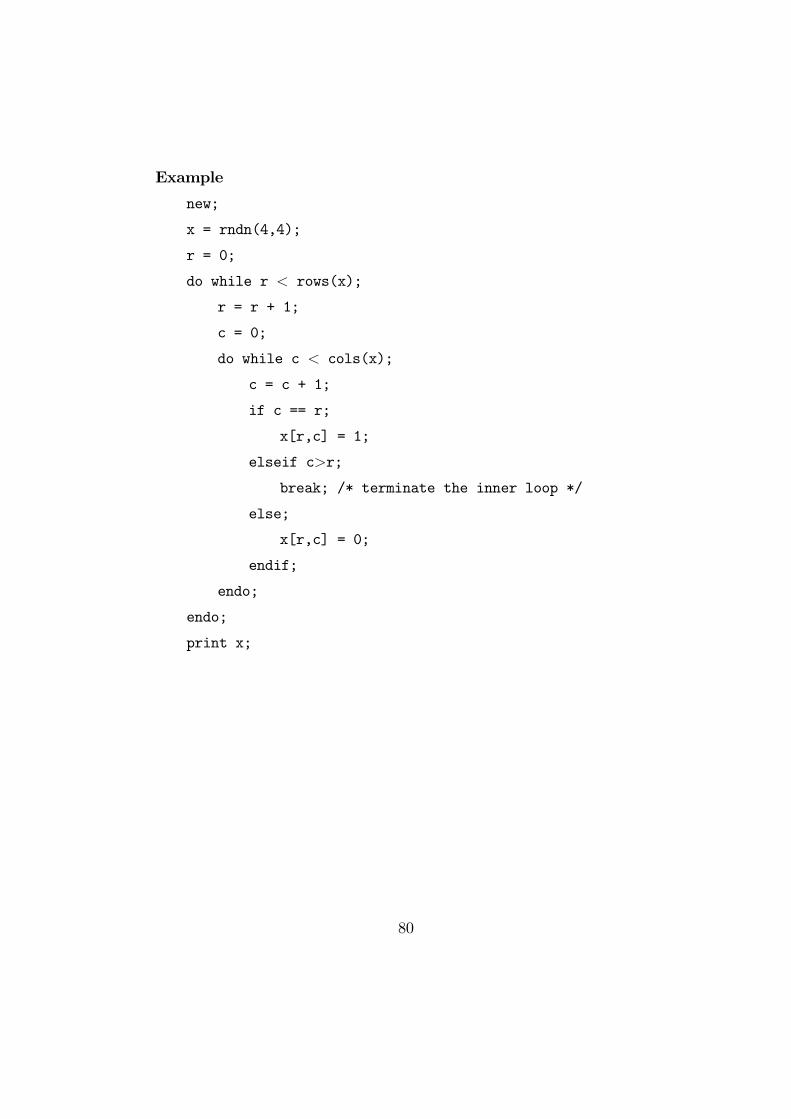
Example
new;
x = rndn(4,4);
r = 0;
do while r < rows(x);
r = r + 1;
c = 0;
do while c < cols(x);
c = c + 1;
if c == r;
x[r,c] = 1;
elseif c>r;
break; /* terminate the inner loop */
else;
x[r,c] = 0;
endif;
endo;
endo;
print x;
80

Example
new;
x = rndn(4,4);
r = 0;
do while r < rows(x);
r = r + 1;
c = 0;
do while c < cols(x);
c = c + 1;
if c == r;
continue;
endif;
x[r,c] = 0;
endo;
endo;
print x;
81

Example
new;
rndseed 123;
s1 = 0;
s2 = 0;
i = 1;
do until i > 100;
e = rndu(1,1);
if e <= 0.48;
print ’’profit’’;
s1 = s1 + 1;
elseif e <= 0.96;
print ’’loss’’;
s2 = s2 + 1;
else;
print; print;
print ftos(i,’’for i = %lf, we restart’’,1,0);
print;
continue;
endif;
if abs(s1 - s2) > 10;
print; print;
print ftos(i,’’the game is stopped for i = %lf, we restart’’,1,0);
break;
endif;
i = i + 1;
endo;
82

20.2.3 FOR loops
A FOR loop cycles a fixed number of times. In this it differs from the WHILEloop, which checks the end condition on every cycle. Because of this, the FORloop operates much more quickly.The format of the FOR loop is
FOR i(start, stop, interval);:ENDFOR;
• The for statement is faster than the do while and do until state-ments. However, its functionality is more limited. It uses only integersas the loop index whereas anything, an integer, complex number, ra-tio, string, or matrix, may be used as the loop index in a do whileor do until loop. The for loop stops only when the specified limitvalue is exceeded. Stopping conditions for the do while and do untilloops are more general; anything may be specified. Finally, recursiveprocedure calls are allowed in do loops but not in for loops.
• The variables start, stop, and interval control the number of timesthe loop operates. The loop will count from start to stop in stepsof interval. Unlike the WHILE loop, there is no need to reset thecounter explicitly.
• The counter i can be referenced within the loop, but should not bechanged. The counter is also local to the loop. That is, if not pre-existing when the loop starts it is created; it is controlled by theloop properties; and on exiting the loop (whether normally or throughBREAK) the value is undefined.
20.2.4 FOR examples
To rewrite the above code to count down to zero using a FOR loop, then
Example
FOR i (10, 1, -1);
PRINT i;;
ENDFOR;
83
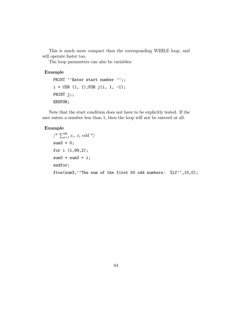
This is much more compact then the corresponding WHILE loop, andwill operate faster too.The loop parameters can also be variables:
Example
PRINT ’’Enter start number ’’;;
i = CON (1, 1);FOR j(i, 1, -1);
PRINT j;;
ENDFOR;
Note that the start condition does not have to be explicitly tested. If theuser enters a number less than 1, then the loop will not be entered at all.
Example
/*P99
i=1 xi, xi odd */
sum3 = 0;
for i (1,99,2);
sum3 = sum3 + i;
endfor;
ftos(sum3,’’The sum of the first 50 odd numbers: %lf’’,10,0);
84
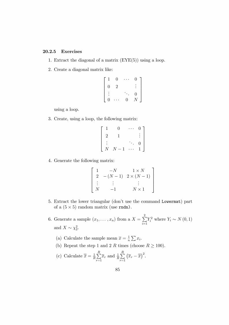
20.2.5 Exercises
1. Extract the diagonal of a matrix (EYE(5)) using a loop.
2. Create a diagonal matrix like:1 0 · · · 0
0 2...
.... . . 0
0 · · · 0 N
using a loop.
3. Create, using a loop, the following matrix:1 0 · · · 0
2 1...
.... . . 0
N N − 1 · · · 1
4. Generate the following matrix:
1 −N 1×N2 − (N − 1) 2× (N − 1)...
......
N −1 N × 1
5. Extract the lower triangular (don’t use the command Lowermat) partof a (5× 5) random matrix (use rndn).
6. Generate a sample (x1, . . . , xn) from a X =2Pi=1
Y 2i where Yi ∼ N (0, 1)and X ∼ χ22.
(a) Calculate the sample mean x = 1n
Pxi.
(b) Repeat the step 1 and 2 R times (choose R ≥ 100).
(c) Calculate x = 1R
RPr=1
xr and 1R
RPr=1
¡xr − x
¢2.
85

(d) Evaluate
1
R
RXr=1
xr − E£χ22¤
1
R
RXr=1
¡xr − x
¢2 − V ar £χ22¤ /nTheorem 7 Sampling Distribution of the Sample Mean. If (x1, . . . , xn)are a random sample from a population with mean µ and varianceσ2, then x is a random variable with mean µ and variance σ2/n.
7. Sample n observations from the t distribution with d degrees of freedomby sampling d+1 values from the standard normal distribution andthen computing
tir =zir,d+1s1d
dPj=1
z2ir,j
i = 1, . . . , n j = 1, . . . , R
where d = 6, 8, 20 and n = 10, 20, 30.
(a) Generate, for each value of n and d, R=100 replications.
(b) Calculate for each of the 100 replications the mean and the me-dian.
(c) The mean and the median are unbiased estimators, so comparethe mean squared errors using,
Mn,d =
1R
RPr=1
(medianr − 0)2
1R
RPr=1
(xr − 0)2
86

20.3 Suspending execution: PAUSE, WAIT and END
All these commands stop execution either temporarily or permanently. Inaddition, some key combinations may stop a program in an emergency.
20.3.1 Temporary suspension using commands
Three commands can lead to the temporary suspension of a program:
PAUSE (sec);WAIT;WAITC;
PAUSE will wait for sec seconds before the program continues.
WAIT will wait until a key has been pressed.
WAITC will clear the keyboard buffer before waiting for a key, so that theprogram will always stop long enough for, for example, a message tobe read. In this, WAITC works much the same as the MS-DOS ”pause”command.
These functions are most useful where the program is stopped while some-thing is being checked or a message is displayed which should be read.
WAIT and WAITC cannot be used to read console input. The key read byeither of these two is lost to the program. The key is only wanted forits signalling role, not for its inherent value, and GAUSS throws thekey away once the signal has been received.
20.3.2 Terminating a program using commands
When GAUSS has finished executing all the instructions in a file, the pro-gram is finished. However, GAUSS just returns to command mode; all theparameters, environment settings and variables used by the program stillexist and are accessible to either instructions on the command line or newprograms. This is the main reason for calling NEW at the beginning of aprogram: it clears out all the rubbish from any previous work.Having variables around is not a problem. GAUSS could run out of mem-
ory, but as the program is finished this is unlikely to be a serious problem.
87

However, the case for file access is different. Many PCs, and GAUSS, havesome sort of disk cacheing system: a small, fast bit of memory is used as anintermediary store between disk and ”normal” memory to avoid excess diskaccesses. If a GAUSS dataset has been used for writing, then the last set ofchanges may not be permanently written to disk until the file is CLOSEd.Closing a file is the only way to be sure (relatively) that updates are properlywritten to disk. The GAUSS manual is silent on what happens to open fileswhen the GAUSS environment is left. Therefore, in a worst case, runninga program and then leaving the GAUSS system could result in some databeing lost even though the program has run ”correctly”.Ideally, a program should close all files and reset all screen and output
options before it terminates. However, the commandEND;will also carry out these functions. END tells GAUSS that the program
is complete. Even if there are more instructions, the program will terminateat this point. Moreover, the housekeeping functions will ensure that thereis an orderly exit from the program. Neither NEW or END is necessary to aprogram, but between them they increase the security of the program andthe integrity of the GAUSS environment. If several programs are being run,they will also improve efficiency of the programs by keeping the workspacetidy.END can be placed anywhere in a program. Whenever it is encountered,
the program stops. However, ENDs in the middle of a program are rarely agood idea. Having multiple exit points from a program confuses the issue,usually unnecessarily.
An alternative to END isSTOP;This also indicates to GAUSS that execution is finished, but none of the
housekeeping tasks are carried out. This could be used where, for exam-ple, a program had to be stopped in an emergency with files left open forexamination. It is of little practical use. Use END in preference.In GAUSS 5.0, END causes what appears to be an error message to come
up at the end of the program. This can be ignored.
88

21 Publication Quality GraphicsGAUSS Publication Quality Graphics consists of a set of main graphingprocedures and several additional procedures and global variables for cus-tomizing the output.
Four basic parts to a graphics program:
1. HeaderIn order to use the graphics procedure, the pgraph library must beactive. This is done in the library statement at the top of the program.
library pgraph;
graphset;
Graphset resets the graphical global variable to the default state.
2. Data setup
The data to be graphed must be in matrices.
3. Graphics format setup
Most of graphics elements contain defaults which allow the user togenerate a plot without modification. Then defaults may be overridenby the user through the use of global variables and graphics procedures.
The variables that begins with ”_p” are the global control variablesused by the graphics routines.
4. Calling Graphics RoutinesIt is the main graphics routines where all of the work for the graphicsfunctions get done. The graphics routines takes as input the user dataand global variables which have previously been set up.
89
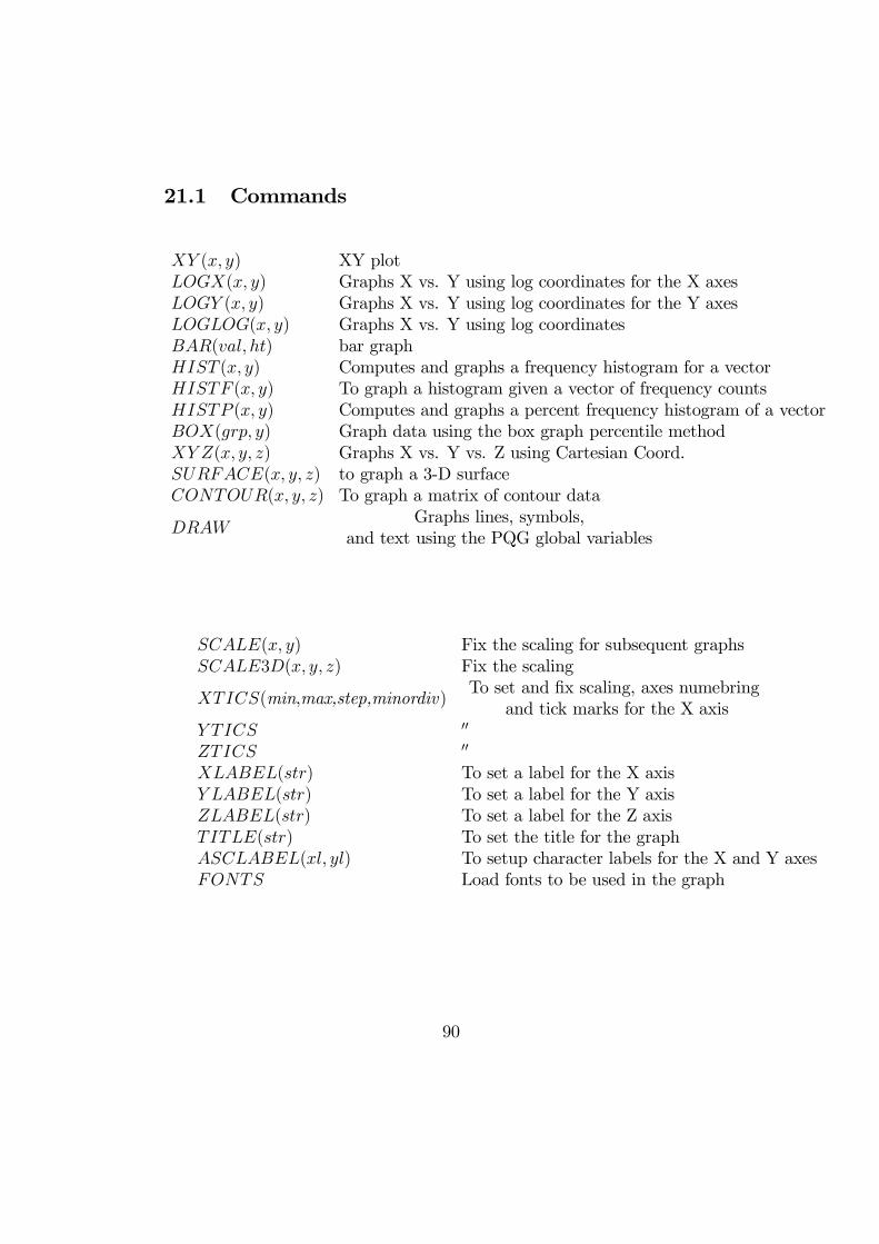
21.1 Commands
XY (x, y) XY plotLOGX(x, y) Graphs X vs. Y using log coordinates for the X axesLOGY (x, y) Graphs X vs. Y using log coordinates for the Y axesLOGLOG(x, y) Graphs X vs. Y using log coordinatesBAR(val, ht) bar graphHIST (x, y) Computes and graphs a frequency histogram for a vectorHISTF (x, y) To graph a histogram given a vector of frequency countsHISTP (x, y) Computes and graphs a percent frequency histogram of a vectorBOX(grp, y) Graph data using the box graph percentile methodXY Z(x, y, z) Graphs X vs. Y vs. Z using Cartesian Coord.SURFACE(x, y, z) to graph a 3-D surfaceCONTOUR(x, y, z) To graph a matrix of contour data
DRAWGraphs lines, symbols,
and text using the PQG global variables
SCALE(x, y) Fix the scaling for subsequent graphsSCALE3D(x, y, z) Fix the scaling
XTICS(min,max,step,minordiv)To set and fix scaling, axes numebring
and tick marks for the X axisY TICS 00
ZTICS 00
XLABEL(str) To set a label for the X axisY LABEL(str) To set a label for the Y axisZLABEL(str) To set a label for the Z axisTITLE(str) To set the title for the graphASCLABEL(xl, yl) To setup character labels for the X and Y axesFONTS Load fonts to be used in the graph
90

21.2 Global variables
_paxes scalar, 2× 1, 3× 1The first element controls the X axis,the second controls the Y axis, and the third will control the Z axis
_paxht scalar, size of axes labels in inches.If 0, a default size will be computed. Default = 0
_pgrid 2× 1 vector to control grid(1, 1)0 no grid1 dotted grid2 fine dotted grid3 solid grid
(2, 1)0 no subdivisions1 dotted lines at subdiv2 tick marks only at subdiv
_plegctl scalar, 1× 4,legend control variable
[1]1 coordinates in plot coord.2 coordinates in inches3 coordinates in pixels
[2] Legend text font size. 1 ≤ size ≤ 9. Default 5[3] x coordinate of lower left corner of legend box[4] y coordinate of lower left corner of legend box
_plegstr string, legend entry textText for multiple curves is separated by a null byte (”\000”)
_plineM× 9 matrix. Each row controls one item to be drawn.If this is zero nothing will drawn.
_pltype scalar or K × 1 vector, line type for the main curvesIf this is a nonzero scalar, all lines will be this type.If scalar 0, line types will be default styles. The default is 01 dashed2 dotted3 short dashes4 closely spaced dots5 dots and dashes6 solid
91

_plwidth scalar or K × 1 vector, line thickness for main curvesDefault=0 (single pixel)
_pnum scalar, 2× 1 or 3× 1 vector for independent control for axes numberingDefault = 10 No axes numbers displayed1 Axes numbers displayed, vertically oriented on Y axis2 Axes numbers displayed, horizontally oriented on Y axis
_pnumht scalar, size of axes numbers in inches.If 0 (default), a size of .13 will be used
_ptitlht scalar, the height of the title characters in inches.If this is 0, a default height of approx. o.13” will be used
92

21.3 Fonts and Special Characters
The escape codes used for graphics text are:
\000 String termination character (null byte)[ Enter superscript mode, leave subscript mode] Enter subscript mode, leave superscript mode@ Interpret next character as literal\20n Select font number n\L create a multiple line title
Four fonts are supplied with PQG: Simplex, Complex, Simgrma and Mi-crob.Fonts are loaded by the command FONTS:
fonts(’’simplex complex microb simgrma’’);
The FONTS command must be called before any of the fonts may beused in text strings.
One of these fonts may be selected by embedding an escape code of theform:
\201 Simplex\202 Complex\203 Microb\204 Simgrma
Default font is Simplex.
93

Examplenew;library pgraph;graphset;an = zeros(12,10);x = seqa(90,1,10);i=1;do until i > rows(x);
y = seqa(1,1,12);a = 0 $+ ’’19’’ $+ ftocv(x[i],2,0) $+ ftocv(y,2,0);an[.,i] = stof(a);
i = i + 1;endo;datem = vec(an);xy(datem,rndn(rows(datem),1)+5);
new;library pgraph;graphset;n = 100;x = seqa(1,1,n);y = sin(pi*x);fonts(’’simplex complex microb simgrma’’);title(’’\201This is the title using Simplex Fonts’’);xy(x,y);title(’’\202This is the title using Complex Fonts’’);xy(x,y);title(’’\203This is the title using Microb Fonts’’);xy(x,y);
new;library pgraph; graphset;t = seqa(0,2*pi/100,100);x = sin(t);_pdate = ’’’’;_pnum = 2;title(’’The sinus function’’);
94

xlabel(’’t’’);ylabel(’’sin(t)’’);xy(t,x);
library pgraph;graphset;n = 100;x = seqa(1,1,n);y = sin(pi*x);fonts(’’simplex simgrma’’);title( ’’\201f(x) = sin(\202p\201x)’’ );xy(x,y);
x = seqa(-3,.01,6/.01);z = sqrt(1/(2*pi))*exp(-(x.^2)/2);title( ’’\201f(x) = \2021\2011/2\202p\201e[-x[2]/2]’’ );xy(x,z);
new;library pgraph;graphset;t = seqa(0,2*pi/100,100);x1 = sin(t);x2 = cos(t);fonts(’’simplex simgrma’’);_pdate = ’’’’;_pnum = 2;title(’’trigonometric functions’’);xlabel(’’t’’);_plegstr = ’’sin(t)\000cos(t)’’;_plegctl = {2 6 4 5};xtics(0,2*pi,pi/2,4);ytics(-1,1,0.5,5);labelx = ’’\2010 \202p\201/2 \202p \2013\202p\201/2 \2012\202p\201’’;
95

labelx = 0 π/2 π 3π22π
asclabel(labelx,0);xy(t,x1~x2);
96

21.4 Windows
A window is any rectangular subsection of the screen or page. Windows maybe of any size and position on the screen and may be tiled or overlapping,transparent and nontrasparent.Tiled windows don’t overlap. The screen can be divided into any number
of tiled windows with
WINDOW(nrows,ncols,attr);
Inputs:
1. number of rows
2. number of columns
3. window type attribute (1=transparent, 0=nontransparent).
Overlapping windows are create with the MAKEWIND command:
MAKEWIND(hsize,vsize,hpos,vpos,attr);
Inputs:
1. horizontal size
2. vertical size
3. horizontal distance from left edge of screen in inches
4. vertical distance from the bottom edge of screen in inches
5. window attribute type (1=transparent, 0=nontransparent)
Screen dimension expressed in inches 9× 6.855
97

begwind Window initialization procedureendwind End window manipulations, display graphswindow Partition screenmakewind Create Window with specified size and positionsetwind Set to specified window numbernextwind Set to next available window numbergetwind Get current window numbersavewind Save Window configurationloadwind Load Window configuration
98
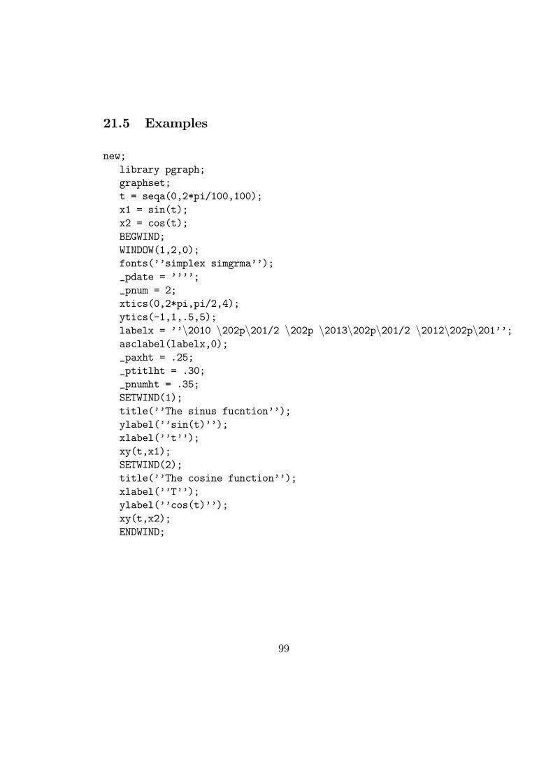
21.5 Examples
new;library pgraph;graphset;t = seqa(0,2*pi/100,100);x1 = sin(t);x2 = cos(t);BEGWIND;WINDOW(1,2,0);fonts(’’simplex simgrma’’);_pdate = ’’’’;_pnum = 2;xtics(0,2*pi,pi/2,4);ytics(-1,1,.5,5);labelx = ’’\2010 \202p\201/2 \202p \2013\202p\201/2 \2012\202p\201’’;asclabel(labelx,0);_paxht = .25;_ptitlht = .30;_pnumht = .35;SETWIND(1);title(’’The sinus fucntion’’);ylabel(’’sin(t)’’);xlabel(’’t’’);xy(t,x1);SETWIND(2);title(’’The cosine function’’);xlabel(’’T’’);ylabel(’’cos(t)’’);xy(t,x2);ENDWIND;
99

new;library pgraph;T = seqa(1,4*pi/101,101);x = cos(t);y = sin(t);z = (x’^2).*y;n = rndn(1000,1);graphset;begwind;makewind(9/2,6.855/2,0,0,0);
MAKEWIND has 5 inputs:
1. horizontal size
2. vertical size
3. horizontal distance from left edge of screen in inches
4. vertical distance from the bottom edge of screen in inches
5. window attribute type (1=trasparent, 0=nontrasparent)
Screen dimension expressed in inches 9× 6.855
The makewind command will create an overlapping window of size 9/2inches horizontally by 6.855/2 inches vertically and positioned 0 inch fromthe left edge of the page and 0 inch from the bottom of the page. It will benon transparent.
makewind(9/2,6.855-1,9/2,1,0);makewind(9/2,6.855/2,0,6.885/2,0);makewind(9/2,6.855/2,0,6.885/2,1);makewind(3,3,3.5,0.25,1);_pdate = ’’’’;
setwind(1);fonts(’’simplex simgrma’’);title(’’Parametric Function’’\
100

’’\Lx = cos(\202t\201),’’\’’ y = sin(\202t\201),’’\’’ z = cos(\202t\201)[2] * sin(\202t\201)’’\4 ’’\L\202t!@[\2010,4\202p@]’’);_paxes = 0;_pframe = 0;_psurf = {0,0};_pzclr = {1,9,4};_ptitlht = .25;volume(3,2,1);surface(x’,y,z);setwind(2);graphset;title(’’Histogram’’);_ptitlht = .20;_pnumht = .20;_paxht = .20;_pnum = 2;call hist(n,100);
101

HIST computes and graphs a frequency histogram for a vector. The actualfrequencies are plotted for each category.
{b,m,freq}=HIST(X,V)
1. X (M × 1) vector of data2. V (N × 1) vector of breakpoints to be used to compute the frequencies,or scalar the number of categories.
setwind(3);title(’’XY Plot’’);xtics(-2,2,1,10);ytics(-2,2,1,10);xy(x,y);setwind(4);xy(2*x,2*y);setwind(5);_ptitlht = .5;_pnum = 0;_paxes = 0;xy(2*x,2*y);endwind;
102

new;x = seqa(-10,0.1,71)’;y = seqa(-10,0.1,71);z = cos(5*sin(x) - y);begwind;makewind(9,6.855,0,0,0);makewind(9/2,6.855/2,1,1,0);setwind(1);_pzclr = {1,2,3,4};title(’’cos(5*sin(x) - y)’’);xlabel(’’ X axis’’);ylabel(’’Y axis’’);scale3d(miss(0,0),miss(0,0),-5/5);surface(x,y,z);nextwind;graphset;_pzclr = {1,2,3,4};_pbox = 15;contour(x,y,z);endwind;
103

22 Input and OutputGAUSS handles data on disk in a number of formats. It can read and createstandard text files and older spreadsheet formats, as well as using its ownformat to store matrices, datasets or code samples.
GAUSS matrices
ASCII files (normal text) anything.
GAUSS datasets .DAT, .DHT (files come in pairs)
Spreadsheets
22.1 GAUSS Matrices
A .FMT file contain a GAUSS matrix. A matrix can be saved onto disk andcan be retrieved at any time. This is the default option - if no extension isgiven to file names, GAUSS will assume it is reading or writing a matrix file.
The commands for matrix files are:
load varname = filename;
loadm varname = filename;
If the disk file has the same name as the variable. Load and loadm aresynonyms.
save filename = varname;
creates a file on disk called filename.fmt which contains the matrix var-name.save varname,
saves the variable varname to a file called varname.fmt.
Example
filename = ’’file1’’;
104

loadm mat1 = ^filename;filename = ’’file2’’;save ^filename = mat1;
This code reads a matrix from file1.fmt and then saves it to file file2.fmt.An alternative is to have the name of the file in a string variable. To tell
GAUSS that the name is contained in the string, the caret (^) operator hasto be used. GAUSS then looks at the current value of the variable to seewhich name to use, instead of taking the variable name as a constant value.This indirect referencing is the more usual way of using file names: it
allows for the program to prompt for names, rather than having them ex-plicitly coded into the program. This is useful when the program does notknow what files are to be used - for example, if a program is to be run onseveral sets of data.
22.2 ASCII files
22.2.1 Reading
Input can be taken from ASCII (i.e. normal alphanumeric text) files usingthe LOAD command described above. This is augmented by the addition ofsquare brackets which indicate the ASCII nature of the file:
load varname[]=filename;
or
load varname[r,c]=filename;
In the first case varname is a (r × c) × 1 vector if filename contains a(r × c) matrix.In the second case varname is a (r × c) matrix. The objects in the file
can be text or numbers, they must be separated by spaces or commas.
loadm filename;
This will load the data in filename in a variable called filename.If the name of the file is a string we have to use ^ to interpret the following
name as a variable.
105

filename = ’’file1’’;loadm x = ^filename;filename = ’’file2’’;save ^filename = mat;
Remark 8 Neither RESHAPE or LOAD[r, c] will send an error message ifthey do not find the correct number of elements to fill the output matrix. Theywill always return a matrix of the desired size. This is why it is important tocheck the number of elements read in before reshaping them into a matrix.
106

Producing ASCII output files is no different from displaying on the screen.GAUSS allows for all output to be copied and redirected to a disk file. Thusanything which appears on the screen also appears in the disk file. To producean ASCII file therefore requires that
1. an output file is opened;
2. PRINT is used to display all the information to go into the output file
3. the output file is closed when no more output is to be sent to it.
The relevant command to begin this process is OUTPUT:
OUTPUT FILE = fileName ON;OUTPUT FILE = fileName RESET;
Both will instruct GAUSS to send a copy of everything it displays, fromthat point onward, to the file fileName. If fileName does not already exist,then these two are identical; but if the file does exist, then the first formensures that any output is appended to the existing contents of the file,while the second empties the file before GAUSS starts writing to it. If nofile name is given, then GAUSS will use the default ”output.out”. There isno default extension for output files.Once a file has been opened, it can be closed and opened any number of
times by combining the above commands withOUTPUT OFF;
These commands will all work on the last recorded file name given. TheFILE=fileName bit could be included here as well if the user wishes to swapbetween different output files; generally, however, only one output file is usedfor a program, and so naming the file explicitly is superfluous.An analogous command SCREEN switches screen output on and off. These
two commands are independent and so screen display off and file output onis a perfectly acceptable combination.
107
22.2.2 Writing
To write data to an ASCII file the print and printfmt commands are used toprint to the auxiliary output. The resulting files are standard ASCII files,and can be edited with any text editor.To write to an ASCII file we have to:
1. open an output file:
output file = filename on; opens the auxiliary output file and causesthe results of all print statements to be sent to that file. If the file al-ready exists, it will be opened for appending. If the file does not alreadyexist, it will be created.
output file = filename reset; It always creates a new file. If thefile already exists, it will be destroyed and a new file by that name willbe created. It it does not exist, it will be created.
Because GAUSS is treating the output as something to be ”displayed”(even if only to a file), it retains the concept of only having a certainnumber of characters on a ”line”. The default is eighty characters,the standard screen width. This means that sending a matrix with alarge number of columns to an output file may lead to the matrix beingbroken up, with ”overflow” columns being put on new lines. The wayto avoid this is to use
OUTWIDTH numChars;
where numChars is the nominal line width, and can be anything from2 to 256. If this is set to 256, then this tells GAUSS to leave out allextraneous line breaks - new lines will only start with a new row of thematrix. Note that output on the screen may still be wrapped around.This does not affect the layout of the output file - it is just the display’sfunctionality, and nothing to do with GAUSS.
2. print the data that we want to write;
3. close the output file:
output off; closes the auxiliary output and turns off the auxiliaryoutput.
108

22.3 Spreadsheets
GAUSS 4.0 and 5.0 for Windows can import data directly from Excel spread-sheets. For multiple-page spreadsheets, you can specify both the sheet andthe cell range to upload. It will try to maintain character and numeric datacharacteristics.GAUSS will also export data to these third-party formats. However,
it writes these data files in the earliest compatible version. For example,although it understands Excel spreadsheets up to version 7, it will save themas version 2.1 by default.
mat = SPREADSHEETREADM(fileName,range,sheet);:okay = SPREADSHEETWRITE(mat,fileName,range,sheet);
In version 4: If the first row contains text, GAUSS assumes that theseare column headings and creates an appropriate matrix of variable names.If it only finds numeric data, it creates a vector of column names as ”C1”,”C2” and so on. When exporting, the situation reverses and you can supplycolumn names.The import command just returns a matrix and it’s up to the user to
break off row or column headings. When writing, particular areas of thespreadsheet can be targetted.Warning: while the obsolete v4.0 commands still exist in v5.0, they only
work correctly if the read spreadsheet has column names. GAUSS 5 assumesthat column names exist and so will automatically chop off the top row. Ifyour spreadsheet file has no column headings, you will lose a row of data.Please also note that although v4.0 starts numbering spreadsheets from
0, v5.0 numbers them from 1:
• EXPORT in v4 returns a 0 if the operation failed; SPREADSHEETWRITEMreturns a 0 if the operation succeeded
• The v5 commands do not appear to work if Excel is not installed onyour computer
• if a full path is not specified, v4 uses the working directory but v5appears to use the system default document directory.
109

Using the import and export functions is much more convenient thanusing ASCII files as intermediaries, as well as being more reliable. However,if you are running your program on something other than GAUSS 4.0+ forWindows, you will need to go back to ASCII files for data exchange.
110

• SpreadsheetreadM
xlsmat = SpreadsheetReadM(file, range, sheet);
Input
file string, name of .xls file.
range string, range to read or write; e.g., ”a1:b20”.
sheet scalar, sheet number.
Output
xlsmat matrix of numbers read from Excel.
If the read functions fail, they will return a scalar error code whichcan be decoded with scalerr. If the write function fails, it returns anon-zero error number.
• Spreadsheetwritexlsret = SpreadsheetWrite(data, file, range, sheet);
Input
data matrix, string or string array, data to write.
file string, name of .xls file.
range string, range to read or write; e.g., ”a1:b20”.
sheet scalar, sheet number.
Output
xlsmat success code, 0 if successful, else error code.
111

Examplenew;y = seqa(1,1,10);x = rndu(10,1);data = y~x;filename = ’’c:\\gauss50\\eser\\gauss2excl.xls’’;range = ’’a1:b10’’;ret = spreadsheetwrite(data,filename,range,1);ret;filename = ’’c:\\gauss50\\eser\\gauss2excl2.xls’’;range = ’’a1:b11’’;xlsmat = SpreadsheetReadM(filename, range, 1);printfm(xlsmat,zeros(1,2)|ones(10,2),fmt);
112

22.3.1 Format
The following commands can be used to control printing to the auxiliaryoutput:FormatControls the format of matrices and numbers printed out with print and
lprint statements.
format /typ /fmted /mf /jnt [f,p]
/mf Matrix row format/m0 no delimiters/m1 or /mb1
print 1 carriage return/line feed pair before each row of a matrixwith more than 1 row
/ma1print1 carriage return/line feed pair after each row of a matrixwith more than 1 row
/a1 print 1 carriage return/line feed pair after each of a matrix/b1 print 1 carriage return/line feed pair before each of a matrix
/jnt Right justified/rd
Signed decimal number in the form [-]####.####,where #### is one or more decimal digits.The number of digits before the decimal pointdepends on the magnitude of the number,
and the number of digits after the decimal point depends on the precision.If the precision = 0 no decimal point will be printed
113

/reSigned number in the form [−]#.##E±###,## is one or more decimal digits depending
on the precision, and ### is three decimal digits/ro
This will give a format like /rd or /re depending onwhich is the most compact for the number being printed.A format like /re will be used only if the exponent value
is less than -4 or greater than the precision.If a /re format is used, a decimal point will always appear.
/rzThis will give a format like /rd or /re depending
on which is the most compact for the number being printed.A format like /re will be used only if the exponent value
is less than -4 or greater than the precision.If a /re format is used, trailing zeros will be suppressed
and a decimal point will appear only if oneor more digits follow it.
Left justified/ld
Signed decimal number in the form [-]####.####,where #### is one or more decimal digits.The number of digits before the decimal pointdepends on the magnitude of the number,
and the number of digits after the decimal point depends on the precision.If the precision = 0 no decimal point will be printed.
If ther number is positive a space characterwill replace the lleading minus sign.
Trailing Character
• s the number will be followed immediately by a space character. (De-fault)
• c The number will be followed immediately with a comma.• t The number will be followed immediately with a teb character.• n No trailing character.
114
f scalar expression, controls the filed widthp scalar expression, controls the precision.
For numeric matrices, p sets the number of significant digits to be printed.For string arrays, p sets the number of characters to be printed.A format statement stays in effect until it is overridden by a new format
statement.The total width of field will be overridden if the number is too big to fit
into space allotted.format /rds 1,0 can be used to print integers with a single between
them, regardless of the magnitudes of the integers.
GAUSS default = format /mb1 /ros 16,8
format /m1 /rd 16,8
new;rndseed 444;x = rndn(3,3);format /m1 /rd 16,8;print x;
The numbers in the matrix X will be printed with a field width of 16spaces per number, and 8 spaces beyond the decimal point.
print 1000*x;format /m1 /rd 1,8;print x;print 1000*x;format /m1 /rd 13,4;print x;print 1000*x;format /mb1 /ros 16,8;
Outwidth nspecifies the width of the auxiliary output. The default is 80 columns.
2 ≤ n ≤ 256.Screen
115

Controls output to the screen.screen on;The results of all print statements will be directed to the screen.screen off;Print statements will not be sent to the screen. Turning the screen off
will speed up execution.screen;It will print ”Screen is on” or ”Screen is off” on the console.
EndTerminates a program. The End statement terminates the program, the
output file will be closed and the screen will be turned back on.
Example
rndseed 124;x = rndn(10,3);format /rd 8,2;outwidth 132;output file = c:\gauss\eser\datatry1.txt reset;screen off;print x;output off;end;
116

22.4 GAUSS Dataset
GAUSS datasets are created by writing data from GAUSS or by taking anASCII file and converting through a stand-alone program called ATOG.EXE(Ascii TO Gauss). As with the datasets for other econometric packages, theyconsist of rows of data split into fields. GAUSS will automatically add .datto the filenames you give, and so there is no need to include the extension.Unlike the GAUSS matrices, reading from or writing to a GAUSS dataset
is not a single, simple operation. For matrices, the whole object is beingmoved into memory or onto disk. By contrast, a GAUSS dataset is used ina number of stages:
1. The file must be opened,
2. it may be read; or written to;
3. when references to the file are finished, it should be closed.
All files used will be given a handle by GAUSS; this is a scalar which isGAUSS’s internal reference for that file. It will be needed for all operationson that file, and so should not be altered. The handle is needed becauseseveral files can be ”open” at one time. Without the file handle, a datasetcannot be accessed, and if the file handle is overwritten then the wrong filemay be used. So be careful with your handles.
22.4.1 Creating new datasets
To start a new dataset for writing, it must be created. This is done by
CREATE handle = filename WITH colnames,columns,type;Handle is the handle GAUSS will return if it is successful in creating
filename.Filename may be a constant like ”file1”, or it may be a string, referenced
using the ^ operator.Colnames is the list of names for the columns (usually a character vector);
columns tells GAUSS how many columns of data there are.Type is the storage precision of the data - integers (2), single precision
(4), or double precision (8).
117

Example
filename = ’’file1’’;let varnames = Date ExchgeRte InterestRte;CREATE handle1 = ^filename WITH ^varnames,3,4;
It prepares a datafile called file1.dat for writing. A header file file1.dhtwill be also created, which records that the datafile should contain fourcolumns, named ”Date” ”ExchangeRate” ”InterestRate” and in single pre-cision (type = 04, Default).Alternatively, matrices may be converted into datasets using the com-
mand
Success = SAVED(variable,filename,colnames);
variable the matrix to be savedsuccess is a scalar variable set to 1 if the operation worked.
118
22.4.2 Opening datasets
A dataset must be opened for either reading or writing or updating (both).Once a dataset has been opened for one mode it cannot be switched toanother.
OPEN handle = filename FOR mode VARINDXI offset;
handle is a non-negative scalar if the operation is successful (if the commanddid not work, the handle is set to -1).
mode = READ,APPEND or UPDATE. (READ = default).
If READ is chosen updating the file is not allowed. Choosing APPENDmeans that the data can only be appended to the file. UPDATE allowsreading and writing.
VARINDXI. WhenGAUSS opens the file, it reads the names of fields (columns)from the .DAT fileand prefixes them all with ”i” (for index). These canthen be used to reference the columns of the dataset symbolically in-stead of using column numbers explicitly.
Offset scalar option shifts all these indexes by a scalar and so is useful if thedata is to be concatenated horizontally to another matrix or dataset.When a file is created it is automatically opened in APPEND mode.
119

22.4.3 Reading and Moving about
A GAUSS dataset is composed of rows of data, and these rows are the basicunit of manipulation. One or more rows is read at a time; data is parcelledup into rows before being written. GAUSS mantains a file pointer whichmantains the current position (i.e. row number) in the file. Generally, asrows are read from or written to the file, the row pointer is moved on. If therow pointer currently points to the start of the file and ten rows are read,the row pointer now indicates that row eleven is the current row.To find out where the pointer currently is
currPos = SEEKR(handle,rownum);
Handle is the handle returned by the OPEN or CREATE.rownum is the rownum to which the file pointer is to be moved. If it is set
to -1, then currpos is the current row number.
To read the data, the command is
datamat = READR(handle,numlines);
which reads numlines rows from the file referenced by handle into thedata matrix datamat. After the read, the file pointer will have been movedon to the point to the first row after the block just read.
22.4.4 Writing
result = WRITER(handle,datamat);
It will add datamat into the file at the current file position. datamatmusthave the same number of columns as the data currently in the file. Resultis the number of times actually written to disk.
120
22.4.5 Closing
Files should always be closed when reading or writing is finished, GAUSSwill automatically do this when leaving the GAUSS environment or when itencounters the END statement.
Files are closed by the CLOSE command:
result = CLOSE(handle);
result =
½0 closed successfully there is no open file attached with this handle
−1 otherwise
If the close worked, then handle should be set to 0.
Example
result = close(handle);if result == 0;
handle = 0;else;print ’’Close failed on file number’’ handle;endif;
Alternative:
Closeall,Closeall handle1,handle2,..,handlen;
121

23 ProceduresProcedures are short self-contained blocks of code. When they are called bythe program, the chain of command within the program switches to the pro-cedure; when the procedure has completed all its operations, control returnsto the main program.
A procedure works in just the same way as code in the main program.So why bother with them? For a number of reasons, of which the main onesare:
Tidiness. An excessively large and complicated program may be difficultto read, understand, and alter. If the program is broken into sepa-rate sections with meaningful procedure names, it becomes much moremanageable.
Repetitive operations. Some functions are used in many places; for ex-ample, the READR operation, or SEQA which creates ordered vectors.The choice is between explicitly programming the same operation sev-eral times, or writing a procedure and calling it several times; usuallythe latter wins hands down.
Security. As the way a procedure interacts with the rest of the environmentcan be more strictly controlled, then procedures are often easier to testand less susceptible to unexpected influences.
The main disadvantage of procedures is the associated efficiency loss andthe extra memory usage. The first is due to the overhead of setting upsubroutines and variables, and GAUSS seems to manage this relatively well.The second drawback is largely due to the need to take copies of variables,and it is the programmer’s responsibility to minimise this.
122

23.1 Global and local variables
A variable always has a certain scope: the domain in which it is visible(accessible) to parts of a program. All of the variables considered so far havebeen global: they are visible to all parts of the program.Procedures allow the use of local variables: they can only be seen within
the ambit of the procedure. Anything outside that procedure cannot reador access those variables; as far as the program outside the procedure goes,that variable does not exist.
Local variables are only visible at the level at which they were declared.Procedures may be nested: one procedure may call another. However, thelocal variables are only visible to those procedures in which they were called:they are not visible to procedures they call or were called by.Because procedures cannot see the variables created by other procedures,
variables with the same name can be used in any number of procedures. If,however, variable names do conflict, (a global variable has the same name asa local variable), then the local variable always takes precedence.
Local variables only exist for the life of the procedure; once the procedureis completed and control returns to the calling code, all variables local to thatprocedure will be deleted from memory. If the procedure is called again, thelocal variables will be a completely new set, not the set that was used lasttime the procedure was called. Obviously, local variables always start offuninitialised.Global variables cannot be declared inside a procedure. They may be
used, their size may be changed, but they may not be declared afresh. Anyvariable which is used in a procedure must be either declared explicitly as alocal variable or be a preexisting global variable.
123

23.2 Writing procedures
A procedure definition consists of five parts:
1. Procedure declaration: proc statement
2. Local variable declaration: local statement. These are variables thatexist only when the procedure is executing. They cannot con ict withother variables of the same name in your main program or in otherprocedures.
3. Body of procedure
4. Return from procedure: retp statement
5. End of procedure definition: endp statement
PROC (numReturns) = ProcName( inParam1, inParam2,... inParamN);LOCAL locVar1;:LOCAL locVarN;
instruction1;instruction2;:instructionN;RETP(outParam1, outParam2, ... outParamN);ENDP;
proc sqrtinv(x); @ procedure declaration could also be: proc sqrtinv(x);@
local y; @ local variable declaration @y = sqrt(x); @ body of procedure @
retp(y+inv(x)); @ return from procedure @endp; @ end of procedure @
• The first element tells GAUSS that the procedure can be referred to asProcName, that it will return numReturns variables to the bit of codewhich called the procedure, and that it requires a number of piecesof information from the calling code: inParam1 to inParamN. GAUSS
124

will check numReturns against the number of variables actually beingreturned to the calling code and produce an error message if the twodo not match. It will not check that the variables are the right sortof vector, matrix, etcetera. If you have just one return value, you canomit numReturns but I leave it in for consistency.
• The input parameters are variables which can be used like any other.They are copies of the variables with which the procedure was called.Therefore they can be altered in any way inside the procedure and thiswill have no effect on the original variables.
• Local variables are declared using the LOCAL statement. Any vari-ables used in the procedure which are not input parameters or globalvariables must be declared here. variables can be defined in two ways:
LOCAL x;
LOCAL y;
LOCAL z;
or
LOCAL x, y, z;
Note that there is no information about the size or type of the variablehere. All this statement says is that there are variables x, y, and z whichwill be accessed during this procedure, and that GAUSS should addtheir names to the list of valid names while this procedure is running.
• LET statements are legal in a procedure, once the variables have beenidentified as local, global, or parameter.
• The main body of the procedure can contain exactly the same instruc-tions as any other section of code, with the obvious exception thatprocedures cannot be defined within another procedure. However, aprocedure can call other procedures; the only effective limit to thenumber of nested procedure calls is the amount of memory available.
• When the workings of the procedure are finished, the final action isto return to the calling code any output parameters. These can beof any type; GAUSS will not check. Nor will its compiler check warnif the number of returns is not equal to numReturns in the procedure
125

declaration. GAUSS will only report an error when the procedure isactually called during a program run, so a program may run for aconsiderable time before an error in the number of returns is discovered.
• The RETP statement is followed by a list of output parameters. Theseparameters can be any of the variables used.
• If there is no value to be returned, then the RETP statement can beomitted. The procedure can have several RETPs; however, this is notrecommended for the same reasons that multiple END statements area poor idea: they confuse the flow of control, and rarely lead to moreefficient programs. A RETP will usually be the penultimate line of theprocedure.
• The statement ENDP tells GAUSS that the definition of the procedureis finished. GAUSS then adds the procedure to its list of symbols. Itdoes not do anything with the code, because a procedure does not, initself, generate any executable code. A procedure only ”exists” in anymeaningful sense when it is called; otherwise it is just a definition. Con-sider a procedure which is not called during a particular run of a pro-gram. Then that procedure could have contained any code statementsand it would have made no difference whatsoever to the running of theprogram; for all intents and purposes, that procedure was completelyignored and might as well have been just another unused variable. Thisis why local variables have no existence outside their procedure: access-ing variables local to a procedure that was never called is equivalent tobeing the child of parents who never existed.
126

ExampleConsider this simple procedure to take a column vector and fill it with as-
cending numbers. The start number and increment are given as parameters.This mimics the action of the standard function SEQA:
PROC(1) = FillVec(inVec, startNum, step);LOCAL i;LOCAL nRows;nRows = ROWS (inVec);inVec[1] = startNum;i = 1;DO WHILE i <= nRows;inVec[i] = inVec[i-1] + step;i = i + 1;ENDO;RETP (inVec);ENDP;
This procedure could be called by, for example,
sequence = FillVec(ZEROS(10, 1), 10, 10);
which would give a (10× 1) vector counting to one hundred in tens.In this case, even though the parameters are variables within the pro-
cedure, they were created using constants. This is due to the fact thatparameters are copies of the variables passed to the procedure. In the aboveexample, GAUSS calculated the results of the ZEROS operation; createdthree new variables, ”inVec”, ”startNum”, and ”step”, which have no fur-ther connection to the original values ZEROS(..), 10, 10; and then made thesenew variables visible to FillVec, and FillVec only. Thus to concatenate anindex vector onto an existing matrix, a program could use
temp = FillVec(mat[.,1], 1, 1);mat = mat ~temp;
or, equivalently and without needing an extra variable,
mat = mat ~FillVec(mat[.,1], 1, 1);
127

The column of mat used as the input vector is irrelevant; it will not bealtered by the procedure call.Note that when a procedure returns a single result, it can be treated
like the result of any other operation. Thus, given a vector iVec, a validcommand could be
result = SQRT((FillVec(iVec, 50, 1).*FillVec(iVec, 50, -1))*ONES(50,1));
A procedure is called the same way as an intrinsic function.{zed, state1} = rndKMn(3,3,-1); @ this statement defines the input
argument to the procedure @zsi = sqrtinv(zed); @ this statement calls the procedure @
The procedure with two returns would be called as:
{zed, state1} = rndKMn(3,3,-1); @ this statement defines the inputargument to the procedure @{ret1, zsi } = sqrtinvA(zed); @ this statement calls the procedure
@
128

ExampleConsider a procedure which, given a GAUSS dataset handle, reads a
number of lines or returns an end-of-file message:PROC (2) = Extract (handle, numLines);LOCAL currRow;LOCAL readOkay;LOCAL data;currRow = SEEKR (handle, -1);IF (currRow+numLines-1) > ROWSF(handle);readOkay = 0;CLEAR data;ELSE;readOkay = 1;data = READR (handle, numLines);ENDIF;RETP (readOkay, data);ENDP;
Note the need to CLEAR data: if we did not assign some value to data(in this case, 0) before we returned from the procedure, then GAUSS wouldreport an error arising from an uninitialised variable.
129

23.3 Global Variables in External Procedures
Often procedures reference global variables, variables that exist in the globalsymbol table. Each procedure has its own local symbol table which vanishesafter the procedure returns. The global variables in the main symbol tablecan be seen using the show command.Global variables that do not already exist in the symbol table must be
declared and initialized prior to being used. The compiler learns that globalvariables exist from external statements, usually in .ext les. These les tellthe compiler that a variable exists and that it is external to the procedure.For example, suppose a collection of procedures in a file calledmyprocs.src
use a global variable, _myprocs_x. The myprocs.ext file contains:
external matrix _myprocs_x; @ convention is to precede globals with”_” @
Each entry in the .ext file must be initialized in a corresponding .dec file.A .dec file is where values are assigned to global variables at compile time,using declare statements, . The default initialization value for matrices iszero. The default initialization value for strings is a null string. For example,the initialization statement for the _myprocs_x variable looks like this:
declare matrix _myprocs_x; @ This takes the default value of zero @
Suppose there are two matrices and that you want to explicity assignvalues to them compile time. Your .dec file will contain the following lines:
declare matrix _myprocs_x = 3;declare matrix _myprocs_y = { 1.2, 3, -1 };
130

23.4 Procedures as variables
An extremely useful feature of GAUSS is the ability to pass procedures asvariables to other procedures. For example,
PROC(1) = Sign(mat, procVar);LOCAL procVar: proc;LOCAL temp;temp = procVar(mat);IF temp <0;temp = ’’negative’’;ELSE;temp = ’’non-negative’’;ENDIF;RETP (temp);ENDP;
This procedure takes a procedure variable called procVar and a matrixmat as parameters. We need to declare in the procedure body that procVaris a procedure (by the LOCAL procVar: proc; statement) so that GAUSSwill realise this is a procedure and not another matrix or string.Having done that, we can then use procVar within the procedure as if it
were a proper procedure, even though we have no idea what the procedureis. All we require is that procVar takes one input parameter and returns onenumeric scalar.To use this, we need to call it with a reference to the relevant function.
We do this by putting an ampersand & in front of the function name.To continue this example, we could call the above procedure thus:
v = someVector;PRINT ’’The sign of the largest number is ’’ Sign(v, &Max_mat);PRINT ’’The sign of the smallest number is ’’ Sign(v, &Min_mat);
assuming the procedures Max_mat and Min_mat have been defined as tak-ing a vector input and producing a scalar output. So calling any one of thesefunctions with a vector parameter satisfies the requirements of the procedurevariable procVar.GAUSS does not allow GAUSS reserved words (such as MINC) to be
used as procedure variables, although some standard GAUSS procedures can
131

be used. The list of proscribed procedures can be found in the User Guide -Reserved Words Appendix. Anything not in there can be used as a procedurevariable.These are trivial examples, but third-party products make extensive use
of procedure variables - this is how they can supply generic optimisationroutines while you just supply functions and derivatives. If you plan to usethese add-on packages, it is worthwhile practising using procedure variables.
132

Example&F is not a procedure but a scalar it allows to recover the position of F.
new;
proc F(x);local y;y = x^2;retp(y);endp;
proc G(x);local y;y = x^2.*sin(x);retp(y);endp;
proc H(x);local y;y = x^2;retp(y);endp;
points = &F|&G|&H;
proc VE(x,i);local f;f = points[i];local f:proc;retp(F(x));endp;
z = zeros(rows(points),1);x = 2;
133

i = 1;do while i <= rows(points);
z[i] = VE(x,i);i = i + 1;endo;print z;
134
24 Functions and keywordsFunctions are one-line procedures which return a single parameter. They aredefined slightly differently:
FN fnName(inParam1,... inParamN) = someCode;
but otherwise operate in much the same way as procedures. However,the code in a function can only be one line, and functions do not have localvariables. Thus functions can be neater than procedures for defining simplerepetitive tasks, but apart from that they offer no real benefits.Keywords take a single string as input and do not return any output.
They can be useful for printing messages to the screen, for example. Theyare called slightly differently to procedures and functions, looking more likethe PRINT function. They do allow for local variables and more than oneline of code, so in that sense they are more flexible than functions. However,only taking a string as input restricts their value somewhat.
keyword what(str);print ’’The argument is:’’ str ;
endp;what GAUSS;
135

25 Exercises1. Write a procedure to simulate a matrix of Bernoulli random variables.
2. Write a procedure to simulate a matrix of Binomial random variables.
3. Write a procedure to compute a covariance matrix from data; simulatea data set and compute its covariance matrix.
4. Write a procedure to compute a correlation matrix from a covariancematrix.
136

26 Procedures: examples
26.1 Ordinary least squares
Y = Xβ + ²
X (N × k)
ρ (X) = k
E [² |X ] = 0
E [²²0 |X ] = σ2²IN
yt = β0 + β1x1t + . . .+ βkxkt + ²t
Parameters to estimate: (β0,σ2²)0
The OLS estimator of β
argminβ
S (β) = (Y −Xβ)0 (Y −Xβ)
X0b²= 0→ TXt=1
b²t = 0bβ=(X0X)−1X0Y
bY = Xbβb² = bY −Xbβbσ2² = b²0b²
T − k
137

Cov³bβ´ = bσ2² (X0X)−1
t³bβi´ = bβiqbσ2² (X0X)−1ii
R2 =
PNi=1 (byt − y)2PNi=1 (yt − y)2
= 1−PN
i=1b²2tPNi=1 (yt − y)2
138

new;library pgraph;/* Data Simulation */n = 100;x0 = ones(n,1);x1 = seqa(0.02,0.001,n)+.4*rndn(n,1);x2 = sin(seqa(1,1,n)/n+rndu(n,1));x3 = seqm(0.2,0.02,n)+.2*rndn(n,1);t = seqa(1,1,n);xy(t,x1~x2~x3);let beta[4,1] = 2,0.6,-1.7,0.5;y = (x0~x1~x2~x3)*beta + rndn(n,1);xy(t,y);dati = y~(x0~x1~x2~x3);save datimqo = dati;
/* OLS Estimate */
load dati = c:\gauss\eser\datimqo;y = dati[.,1];x = dati[.,2:cols(dati)];Nobs = rows(y);k = cols(x);betah = invpd(x’x)*x’y;yhat = x*betah;epsh = y - x*betah;ssr = epsh’epsh;tss = (y - meanc(y))’(y - meanc(y));rss = (yhat - meanc(y))’(yhat - meanc(y));betah;r2 = rss/tss;r2;gdl = Nobs - k;sigmah = ssr/gdl;Mcov = (sigmah)*invpd(x’x);stderr = sqrt(diag(Mcov));tstud = betah./stderr;
139

pvalue = 2*cdftc(abs(tstud),gdl);deps = epsh - lag1(epsh);deps = trimr(deps,1,0);dw = sumc(deps^2)/sumc(epsh^2);print ftos(Nobs,’’Observation Number: %lf’’,5,0);print ftos(k,’’Number of regressors: %lf’’,5,0);print;print ftos(gdl,’’Degrees of Freedom: %lf’’,5,0);print;print ftos(sigmah,’’Variance Estimate: %lf’’,5,0);print;print ftos(DW,’’Durbin-Watson: %lf’’,5,0);print;print ’’ coefficient stand. error test t marginal prob’’;print’’--------------------------------------------------’’;print betah~stderr~tstud~pvalue;print;print ’’Estimator Var-Cov Matrix’’ Mcov;
Transform this program in a procedure.
140

26.2 Runge - Kutta Algorithm
K Differential Equations of order 1:
dx1dt= f1 (t, x1 (t) , . . . , xk (t))
...dxidt= fi (t, x1 (t) , . . . , xk (t))
...dxkdt= fk (t, x1 (t) , . . . , xk (t))
Vector representation:
dx (t)
dt= f (t,x (t))
x (t) =
x1 (t)...xk (t)
f (t,x (t)) =
f1 (t, x1 (t) , . . . , xk (t))...fk (t, x1 (t) , . . . , xk (t))
h discretization step. xi numerical solution to x (ti), where ti = t0+ ih. Thealgorithm solves
xi+1 = xi +h
6[k1 + 2k2 + 2k3 + k4]
k1 = f (ti, xi)
k2 = f
µti +
h
2, xi +
h
2k1
¶k3 = f
µti +
h
2, xi +
h
2k2
¶k4 = f
µti +
h
2, xi +
h
2k3
¶/*Format{t,x,dx} = RuKu4(&f,xstart,tstart,tend,N):**
141

PurposeIntegrate a system of ODE using the Algortithm of Runge-Kutta
of order 4**** Input &f - pointer to a procedure that computes f(t,X)** Xstart - Kx1 vector, initial value for X** tstart - scalar, initial time value** tend - scalar, number of points**** Output t - Nx1 vector, time** x - Nxk, numerical solution of x(t)** dx - Nxk matrix, numerical solution of dx(t)/dt*/proc(3) = RuKu4(&f,Xstart,tstart,tend,N);local f:proc;local h,t,h2,K,x,dx;local i,ti,xi,dxi;local k1,k2,k3,k4,k5;h = (tend-tstart)/(n-1);t = seqa(tstart,h,N);h2 = h/2;K = rows(Xstart);x = zeros(K,N);xi = Xstart;x[.,1] = xi;dx = zeros(K,N);dx[.,1] = miss(zeros(K,1),0);i = 2;do until i>N;ti = t[i-1];k1 = f(ti,xi);k2 = f(ti+h2,xi+h2*k1);k3 = f(ti+h2,xi+h2*k2);k4 = f(ti+h,xi+h*k3);dxi = (h/6)*(k1+2*k2+2*k3+k4);xi = xi + dxi;x[.,i] = xi;dx[.,i] = dxi;
142
i = i + 1;endo;x = x’;dx = dx’;dx = dx/h;retp(t,x,dx);endp;/***** Example of application of Runge-Kutta4** dx(t)/dt = sin(t)** x(0) = 1.5 - cos(t)***/library pgraph;proc f(t,x);retp(sin(t));endp;t = seqa(1,1,10);{t,x,dx} = RuKu4(&f,.5,0,10,1000);solut = 1.5 - cos(t);graphset;_pdate = ’’’’;title(’’ODE solution: dx/dt = sin(t), x(0) = .5’’);xlabel(’’t’’);ylabel(’’x(t)’’);xy(t,x~solut);
143

Black & Scholes Option Pricing
C = S0Φ (d1)− ke−rτΦ (d2)
d1 =ln (S0/K) + rτ
σ√τ
+1
2σ√τ
d2 = d1 − σ√τ
Φ (·) Gaussian CDF.
Proc EBSCALL(S0,K,Sigma,tau,r);local W,d1,d2,c;w = sigma.*sqrt(tau);d1 = (ln(S0./K) + r.*tau)./W + .5*W,d2 = d1 - w;c = S0.*cdfn(d1) - K.*exp(-r.*tau).*cdfn(d2);retp(c);endp;
144
26.3 Simulation of Stochastic Differential Equation. Eu-ler - Maruyama Algorithm
SDE:
dX (t) = µ (t,X (t)) dt+ σ (t,X (t)) dW (t)
X (t0) = X0
Algorithm:
xi+1 = xi + µ (ti, xi)h+ σ (ti, xi)√hui
ti = t0 + ih
ui ∼ N (0, 1)
xi simulation of X (ti)
26.4 Simulation of the price of a European Call Option
/**Euler-Maruyama Algorithm
x0 initial conditionmu process parameter (scalar or vector)sigma volatility parameter (scalar or vector)t0 initial dateT final dateN # of discrete intervalsM # of simulations
**/
proc(2) = Eu_Maru(x0,mu,sigma,t0,T,N,M);local mu:proc, sigma:proc;local h,t_,x,k1,u,i,ti,xi;h = (T-t0)/N;t_ = seqa(t0,h,N+1);x = zeros(N+1,M);x[1,.] = x0.*ones(1,M);
145

k1 = sqrt(h);u = rndn(N+1,M);i = 1;do until i > N;ti = t_[i];xi = x[i,.];x[i+1,.] = xi + mu(ti,xi)*h + k1.*sigma(ti,xi).*u[i+1,.];i = i + 1;endo;retp(t_,x);endp;
library pgraph;s0 = 100;k = 98;sigma = .15;tau = 95/365;r = .08;c = EBSCall(s0,K,sigma,tau,r);proc a(t,x);retp(r*x);endp;proc B(t,x);retp(sigma*x);endp;rndseed 1234;Ns = 300;{t,s} = Eu_Maru(S0,&A,&B,0,tau,100,Ns);ST = S[101,.]’;PayOff = (ST - K).*( (St - K) .> 0);Csimul = cumsumc(PayOff) ./seqa(1,1,Ns);graphset;_pdate = ’’’’; _pnum = 2;title(’’Simulazione Monte-Carlo del prezzo di un’opzione call’’\’’\LStudio della convergenza’’);_pline = 1~1~0~C~Ns~C~1~2~10;xlabel(’’Numero di simulazioni’’);ylabel(’’Prezzo’’);
146

ytics(3,7,1,10);xy(seqa(1,1,Ns),Csimul);proc EBScall(s0,k,sigma,tau,r);local w,d1,d2,C;w = sigma.*sqrt(tau);d1 = (ln(s0./k) + r.*tau)./w + .5*w;d2 = d1 - w;c = s0.*cdfn(d1) - k.*exp(-r.*tau).*cdfn(d2);retp(c);endp;
147
26.5 Monte Carlo Simulation to price a European CallOption
The price of the underlying is described by a Geometric Brownian Motion
dS (t) = µS (t) dt+ σS (t) dW (t)
S (t0) = S0
The solution is given by the Feynman-Kac Theorem
C (t0) = e−rτ eE £(S (t)−K)+ |Ft ¤
change of probability measure by Girsanov Theorem. Under the risk neutralprobability measure we have
dS (t) = µS (t) dt+ σS (t) dfW (t)
S (t0) = S0
In order to calculate the solution we can use Monte Carlo simulation
C (t0) ' e−rτ"1
N
NXn=1
(Sn −K)+#
148

library pgraph;s0 = 100;k = 98;sigma = .15;tau = 95/365;r = .08;c = EBSCall(s0,K,sigma,tau,r);proc a(t,x);retp(r*x);endp;proc B(t,x);retp(sigma*x);endp;rndseed 1234;Ns = 300;{t,s} = Eu_Maru(S0,&A,&B,0,tau,100,Ns);ST = S[101,.]’;PayOff = (ST - K).*( (St - K) .> 0);Csimul = cumsumc(PayOff) ./seqa(1,1,Ns);graphset;_pdate = ’’’’; _pnum = 2;title(’’Monte-Carlo Simulation of the Call Option price’’\’’\LConvergence Study’’);_pline = 1~1~0~C~Ns~C~1~2~10;xlabel(’’Simulations number’’);ylabel(’’Price’’);ytics(3,7,1,10);xy(seqa(1,1,Ns),Csimul);proc EBScall(s0,k,sigma,tau,r);local w,d1,d2,C;w = sigma.*sqrt(tau);d1 = (ln(s0./k) + r.*tau)./w + .5*w;d2 = d1 - w;c = s0.*cdfn(d1) - k.*exp(-r.*tau).*cdfn(d2);retp(c);endp;
149

26.6 Simulation of Poisson Process
Let’s consider a sequence of random variables strictly increasing
(Tn)n>0
• with T0 = 0,
I{Tn≤t} =½1 if t ≥ Tn (ω)0 if t < Tn (ω)
We define a counting process as
Nt =Xn≥1I{Tn≤t}
A counting process is a Poisson process if Nt −Ns• is a sequence of independent random variables
• are stationary increments (i.e. the distribution of Nt −Ns is the sameas Nv−Nu where 0 ≤ s < t <∞ and 0 ≤ u < v <∞ and t−s = v−u)
N = {Nt}0≤t≤∞Pr {Nt = n} =
e−λt (λt)n
n!n = 0, 1, 2, . . . λ > 0
/* Simulation of Poisson Process *//*Inputlambda - scalar, Process parametert0 - scalar, starting dateT - scalar, final dateL - scalar, number of discrete stepsK - scalar, number of simulationsOutput.ti - vector (L+1)x1, dates
150

N - matrix (L+1)xK, simulated Poisson processThe i-th simulated process corresponds to the vector N[.,i]*/
proc(2)=poisson(lambda,t0,T,L,K);local h,ti,u,N;
h = (T-t0)/L;ti = seqa(t0,h,L+1);u = rndu(L,k);u = u.< (lambda*h);u = zeros(1,K)|u;N = cumsumc(u);
retp(ti,N);endp;
library pgraph;rndseed 123;L = 1000;t0 = 0;TT = 10;lambda = 5;
{t,N} = poisson(lambda,t0,TT,L,1);{t,N2} = poisson(2,t0,TT,L,1);
graphset;fonts(’’simplex simgrma’’);_pdate = ’’’’;_plwidth = 5;_pnum = 2;title(’’Simulation of Poisson process’’\’’\L\202l\201 = 5 _ _ \202l\201 =2’’);xtics(t0,TT,1,0);ytics(0,50,10,0);xs = t[1:L];xe = t[2:L+1];ys = N[1:L];ye = N2[1:L];
151

e = ones(L,1);xlabel(’’t’’);ylabel(’’N]t[(\202w\201)’’);xy(xs,ys~ye);
152

26.7 Simulation of Diffusion Process with jumps
/* Simulation of diffusion process with jumpsInputx0 - scalar or vector Nsx1, initial value of the process&mu - pointer di una procesura che calcola la funzione mu(t,X)&sigma - pointer to a procedure that calculates the function sigma(t,X)&kappa - pointer to a procedure that calculates the function kappa(t,X)&lambda - pointer to a procedure that calculates the function
lambda(t,X)t0 - scalar, t0TT - scalar, TN - scalar, # of points of discretization of the interval [t0,T]Ns - scalare, number of simulations
Outputt - vector (N+1)x1, dates tixt - matrix (N+1)xNs, simulated diffusion process with jumpsdN - matrix (N+1)xNs, when jump 1, no jump 0.*/
new;proc(3) = salto(x0,mu,sigma,kappa,lambda,t0,TT,N,Ns);local h,t,xt,u,dN,i,xi,ti,dN_,lambda_;local mu:proc, sigma:proc,kappa:proc,lambda:proc;
h = (TT - t0)/N;t = seqa(t0,h,N+1);xt = zeros(N+1,Ns);xt[1,.] = x0.*ones(1,Ns);u = rndn(N,Ns)*sqrt(h);dN = zeros(N+1,Ns);i = 1;do until i > N;xi = xt[i,.];ti = t[i];lambda_ = lambda(ti,xi);
153

dN_ = rndu(1,Ns) .< (lambda_*h);xt[1+i,.] = xi + mu(ti,xi)*h + sigma(ti,xi).*u[i,.] + kappa(ti,xi).*dN_;dn[1+i,.] = dN_;i = i + 1;endo;retp(t,xt,dN);endp;
/*Example
dX (t) = µX (t) dt+ σX (t) dW (t) + k (t) dN (t)
X (0) = 2
k (t) = 1
λ (t,X) =
½1 if t ≤ 5
0.5 otherwise
We can obtain as a by-product the Geometric Brownian Motion justsetting lambda = 0 or kappa = 0.*/
library pgraph;x0 = 2;proc mu(t,x);retp(0.0002*x);endp;proc sigma(t,x);retp(1.09*x);endp;proc kappa(t,x);retp(1);endp;proc lambda1(t,x);retp(0);endp;rndseed 123;
154

{t,x1,dN} = salto(x0,&mu,&sigma,&kappa,&lambda1,0,10,100,1);proc lambda2(t,x);if t <= 5;retp(1);else;retp(.5);endif;endp;rndseed 123;{t,x2,dN} = salto(x0,&mu,&sigma,&kappa,&lambda2,0,10,100,1);xs2 = indexcat(dN[.,1],1);graphset;fonts(’’simplex simgrma’’);_pdate = ’’’’;_pnum = 2;title(’’Geometric Brownian Motion : ’’\’’dX]t[ = \202m\201X]t[dt + \202s\201X]t[dW]t[’’\’’\LJump Process : ’’\’’dX]t[ = \202m\201X]t[dt + \202s\201X]t[ + \202k\201]t[dN]t[’’);xy(t,x1~x2);
155