introduction to fluent - minnesota supercomputing institute
TRANSCRIPT
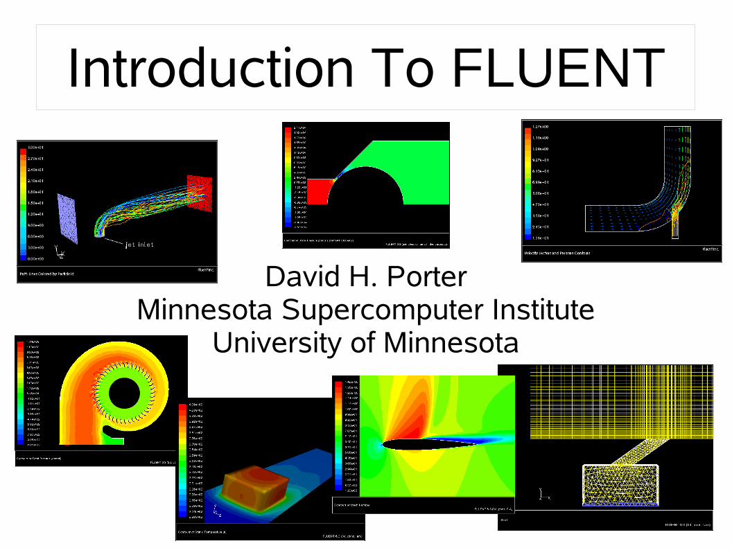
Introduction To FLUENT
David H. PorterMinnesota Supercomputer Institute
University of Minnesota
Topics Covered in this Tutorial
● What you can do with FLUENT– FLUENT is feature rich
– Summary of features and capabilities
● Using FLUENT at MSI– Hosts, X forwarding, environment, startup
● Essentials of working with FLUENT– Basic steps for success
● User Resources at MSI – Web documentation: User Guides & tutorials
– Help is available: helpline & forums
What You Can Do With FLUENT
● Flow problems in 2D and 3D● Compressible & Incompressible● Steady state and time dependent● Variety of material properties● Complex physics & chemsitry● Inviscid, viscous, and turbulence models● Complex geometries & meshes● Multiple and non-inertial reference frames● Quantitative analysis & visualization

Flow Problems in 2D and 3D
● 2D– Planar
– Axisymmetric
– Axisymmetric with swirl
● 3D– Full 3D
– Complex boundaries
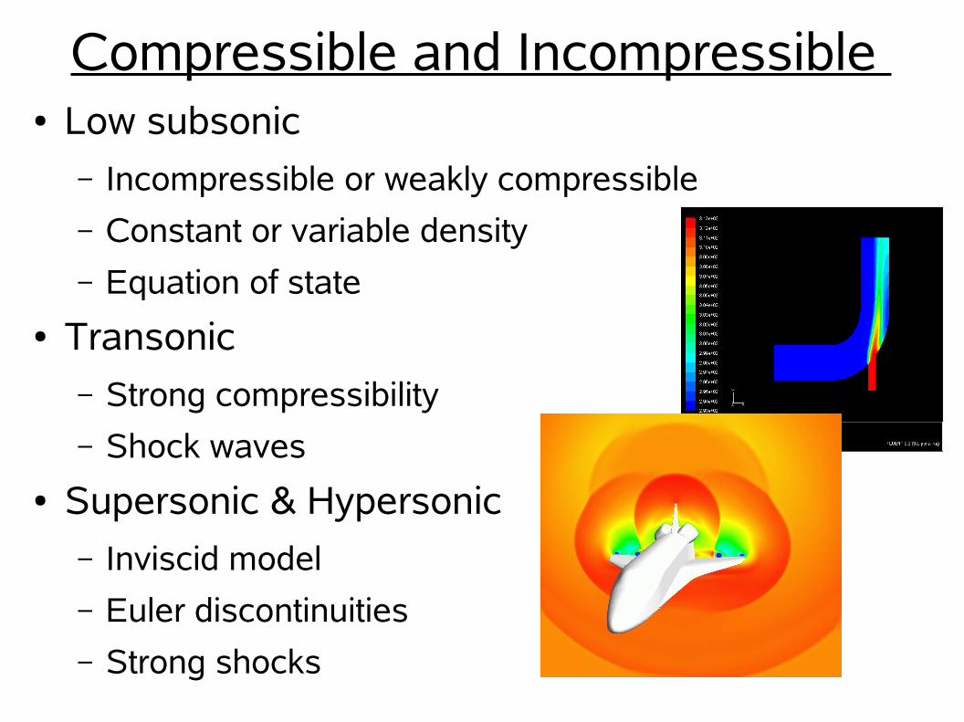
Compressible and Incompressible ● Low subsonic
– Incompressible or weakly compressible
– Constant or variable density
– Equation of state
● Transonic– Strong compressibility
– Shock waves
● Supersonic & Hypersonic– Inviscid model
– Euler discontinuities
– Strong shocks

Steady State and Time Dependent
● Iterative convergence to steady state solutions
● Follow transient solutions
● Use steady state solution to initialize transient problems.

Material Properties● Newtonian & non-Newtonian fluids● Phase changes
– Melting and solidification
● Porous media– Non-isotropic permeability
– Inertial resistance
– Solid heat conduction
– Porous-face pressure jump conditions
● Material properties database
Porous media in a catalytic converter

Chemistry
● Chemical Species– Mixing
– Reaction
● Combustion models– Homogeneous
– Heterogeneous
● Surface deposition/reaction models

Complex Physics
● MHD
● Heat transfer– solid/fluid “conjugate” transfer
– Forced, natural & mixed convection
● Volume sources of mass, momentum and energy
● Acoustic models: flow induced noise
000
Natural ConvectionVelocity field
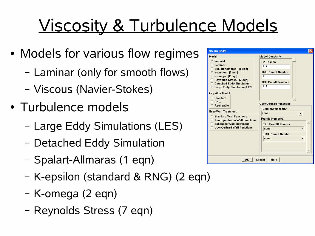
Viscosity & Turbulence Models● Models for various flow regimes
– Laminar (only for smooth flows)
– Viscous (Navier-Stokes)
● Turbulence models– Large Eddy Simulations (LES)
– Detached Eddy Simulation
– Spalart-Allmaras (1 eqn)
– K-epsilon (standard & RNG) (2 eqn)
– K-omega (2 eqn)
– Reynolds Stress (7 eqn)

Complex Geometries & Meshes
● Various and mixed meshes– Structured, unstructured, & mixed
● Sliding meshes● Mixing-plane model
– Time averaged mesh boundaries
● Dynamic (deforming) meshes● Free surfaces● GAMBIT: mesh generation● T-GRID: merge meshes
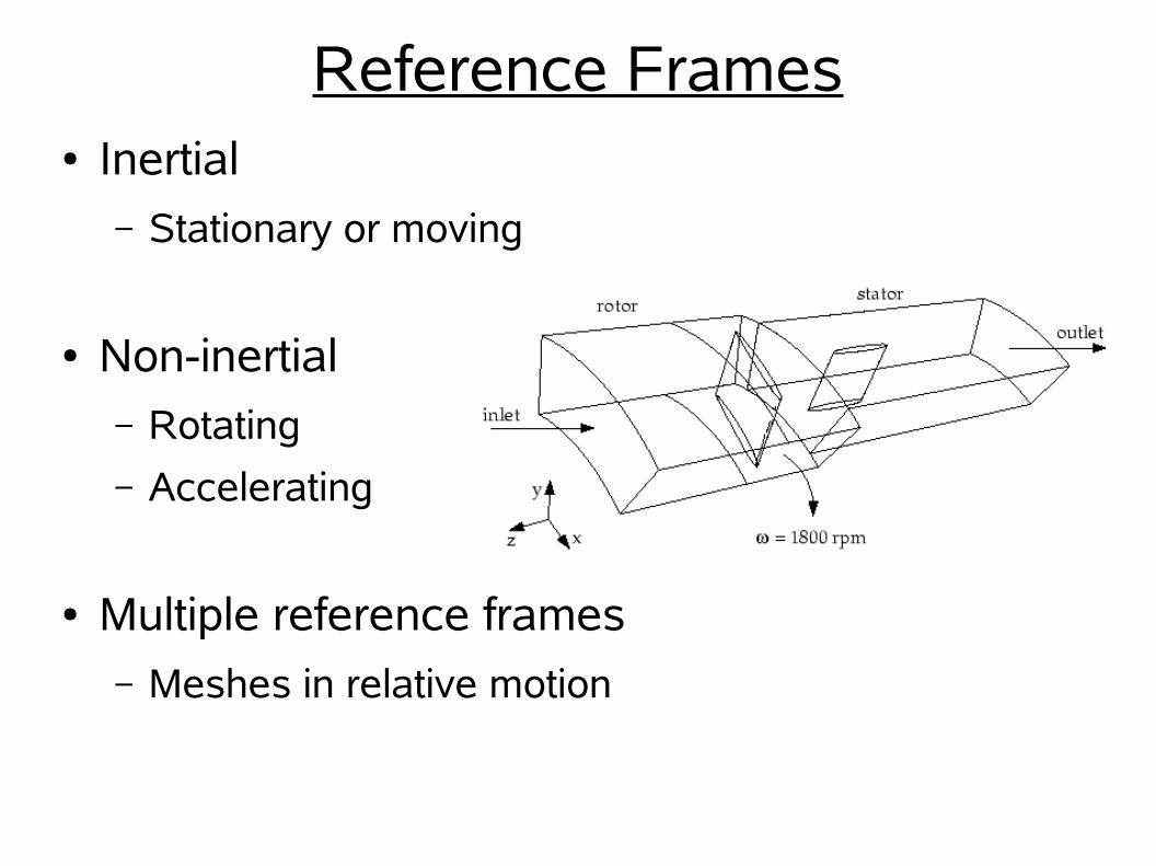
Reference Frames● Inertial
– Stationary or moving
● Non-inertial– Rotating
– Accelerating
● Multiple reference frames– Meshes in relative motion

Quantitative Analysis
● XY plots of values along lines– Primitive & derived
quantities
● Surface and volume integrals– Fluxes
– Averages
● Temporal variation● Fourier analysis

Flow Visualization
● On surfaces– Contours
– Primitive and derived fields
● In volumes– Particle paths
– Vector fields
– Colored with scalar fields
● Animation– Time dependent flows
– Moving viewpoint
Using FLUENT at MSI● Hardware to run FLUENT on
– Computational resources at MSI
– MSI maintains academic licenses from ANSYS
– Run locally in MSI labs
● Running remotely on core hardware– SSH & X forwarding
● Getting Started– Environmental settings & modules
– Tutorial files & run directories
– GUIs for GAMBIT & FLUENT

FLUENT Availability at MSI
● Core hardware (remote access)– Altix (up to 256 processors)
– Regatta (up to 32 processors)http://www.msi.umn.edu/hardware/
● Labs (run locally or remotely)– BMSDL
– SDVLhttp://www.msi.umn.edu/labs/

Running Remotely
● GUI driven GAMBIT & FLUENT● From your graphics & X11 enabled desktop
– X11 is standard with Linux shells
– On Mac use an xterm shell & “ssh -Y ...”
– On Windows, need X server & SSH client● X server: XMing● SSH client: PuTTY
http://www.cs.caltech.edu/courses/cs11/misc/xwindows.html
● Linux: SSH to remote host with X forwarding
ssh -X <user_name>@regatta.msi.umn.edu
Getting Started● Use the “fluent” module to set your environment
module load fluent
● GAMBIT & FLUENT produce many files– Good idea to make a project directory
● Tutorial resource files available on regatta– Meshes & example output
– Zipped files for each tutorial/usr/local/Fluent.Inc/fluent6.3.26/help/tutfiles
http://wwwr.msi.umn.edu/fluent/tutfiles/

Essentials of Working with FLUENT
● Dream up a problem● Draw a picture with labels for consistency● Use GAMBIT to generate mesh
– Specify geometry & boundaries
– Specify solver, mesh type & resolution
● Use FLUENT to generate flow solutions– Specify models, boundaries, material properties
– Specify solver approx, monitors, & iterate ...
– Adapt/refine mesh
– Examine/compare results
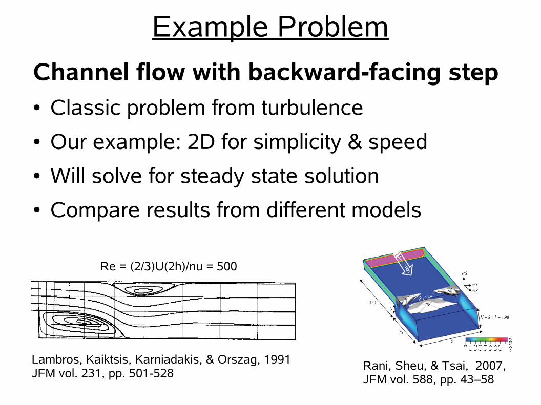
Example Problem
Channel flow with backward-facing step● Classic problem from turbulence● Our example: 2D for simplicity & speed● Will solve for steady state solution● Compare results from different models
Rani, Sheu, & Tsai, 2007,JFM vol. 588, pp. 43–58
Lambros, Kaiktsis, Karniadakis, & Orszag, 1991JFM vol. 231, pp. 501-528
Re = (2/3)U(2h)/nu = 500
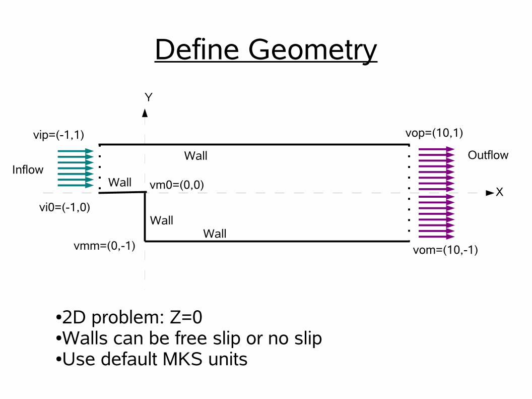
Define Geometry
X
Y
vip=(-1,1)
vi0=(-1,0)
vop=(10,1)
vom=(10,-1)vmm=(0,-1)
vm0=(0,0)Inflow
Outflow
WallWall
Wall
Wall
●2D problem: Z=0●Walls can be free slip or no slip●Use default MKS units

Mesh Generation: Outline● Setup & start GAMBIT● Specify FLUENT 5/6 solver● 0D: Vertices from point coordinates● 1D: Edges from pairs of vertexes● 2D: Domain from edges● Specify 1D meshes on Edges● Interior mesh (on face) from 1D meshes● Associate boundary types & labels with edges● Save work & export mesh

Setup GAMBIT● Project Directory
– Make directory: mkdir step
– Enter directory: cd step
● Start GAMBIT– module load fluent
– gambit
● Specify solver
menu: solver -> FLUENT 5/6

Specify Vertices
● Vertexes from point coordinates– Operation: GEOMETRY button
– Geometry: VETREX button
– Vertex: CREATE VERTEX button
– Enter coordinates with labels & APPLY for each pair
vip (-1,1) vmm (0,-1)
vim (-1,0) vom (10,-1)
vm0 (0,0) vop (10,1)
● Resize view to see all– Global Control: FIT TO WINDOW button
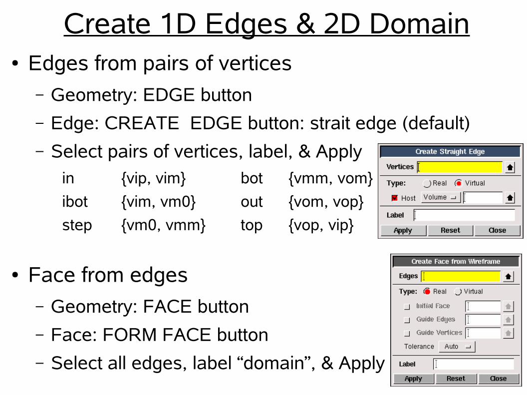
Create 1D Edges & 2D Domain● Edges from pairs of vertices
– Geometry: EDGE button
– Edge: CREATE EDGE button: strait edge (default)
– Select pairs of vertices, label, & Applyin {vip, vim} bot {vmm, vom}
ibot {vim, vm0} out {vom, vop}
step {vm0, vmm} top {vop, vip}
● Face from edges– Geometry: FACE button
– Face: FORM FACE button
– Select all edges, label “domain”, & Apply

Generate Mesh● 1D Mesh on Edges (0.1 m mesh)
– Operation: MESH button
– Mesh: EDGE button
– Mesh Edges dialog:● Spacing: 0.1 (interval size)● Select all edges & Apply
● Mesh 2D domain from edges – Mesh: FACE button
– Face: MESH FACES button
– Mesh faces dialog:● Select all edges● Retain defaults for quad mesh & Apply
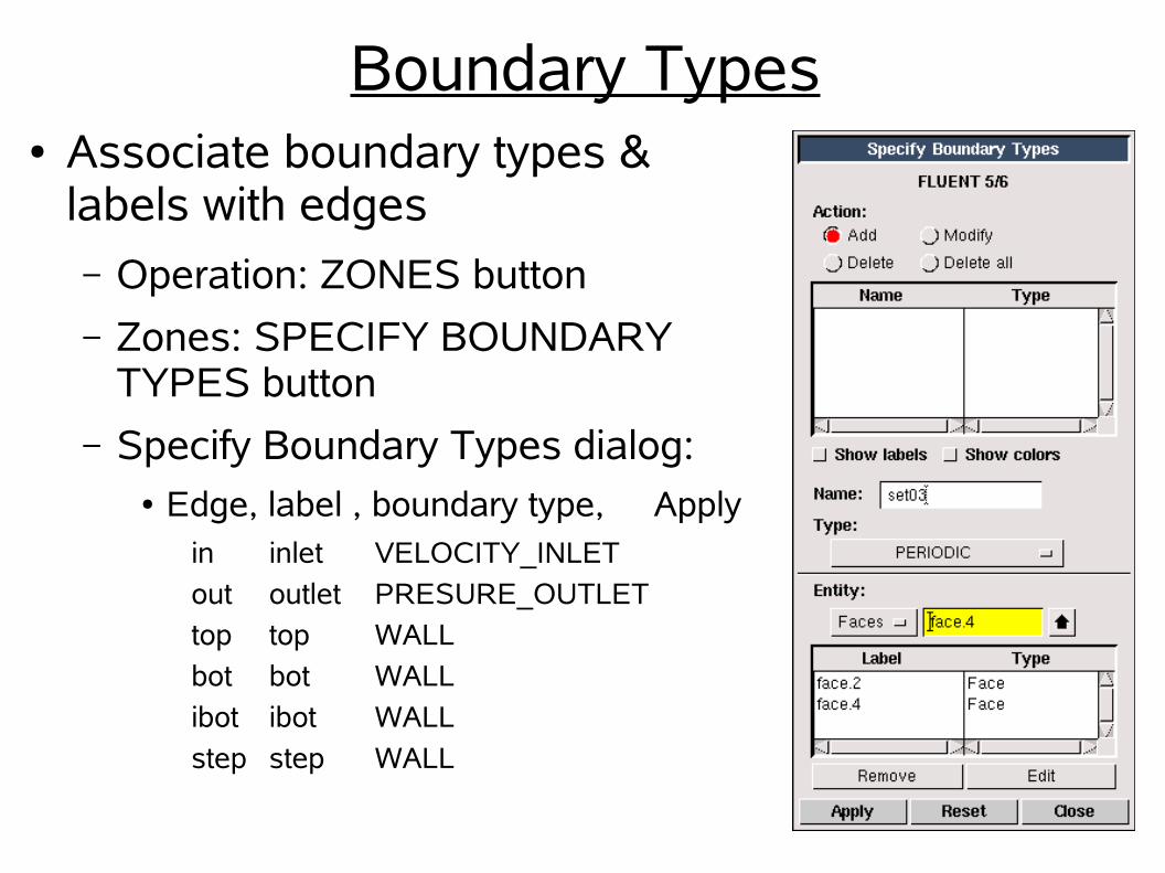
Boundary Types● Associate boundary types &
labels with edges– Operation: ZONES button
– Zones: SPECIFY BOUNDARY TYPES button
– Specify Boundary Types dialog:● Edge, label , boundary type, Apply
in inlet VELOCITY_INLET
out outlet PRESURE_OUTLETtop top WALL
bot bot WALL
ibot ibot WALL
step step WALL

Save Work & Export Mesh● Good Idea to save GAMBIT session
– Modify or fix mesh as needed
– Use as a starting point for another projectMenu: File -> Save As ...
● Export mesh– Generates a mesh file: step.msh
– Will import this file into FLUENTMenu: File -> Export -> Mesh ...● Enable “Export 2-D (X-Y) Mesh”● File name: step.msh● Accept
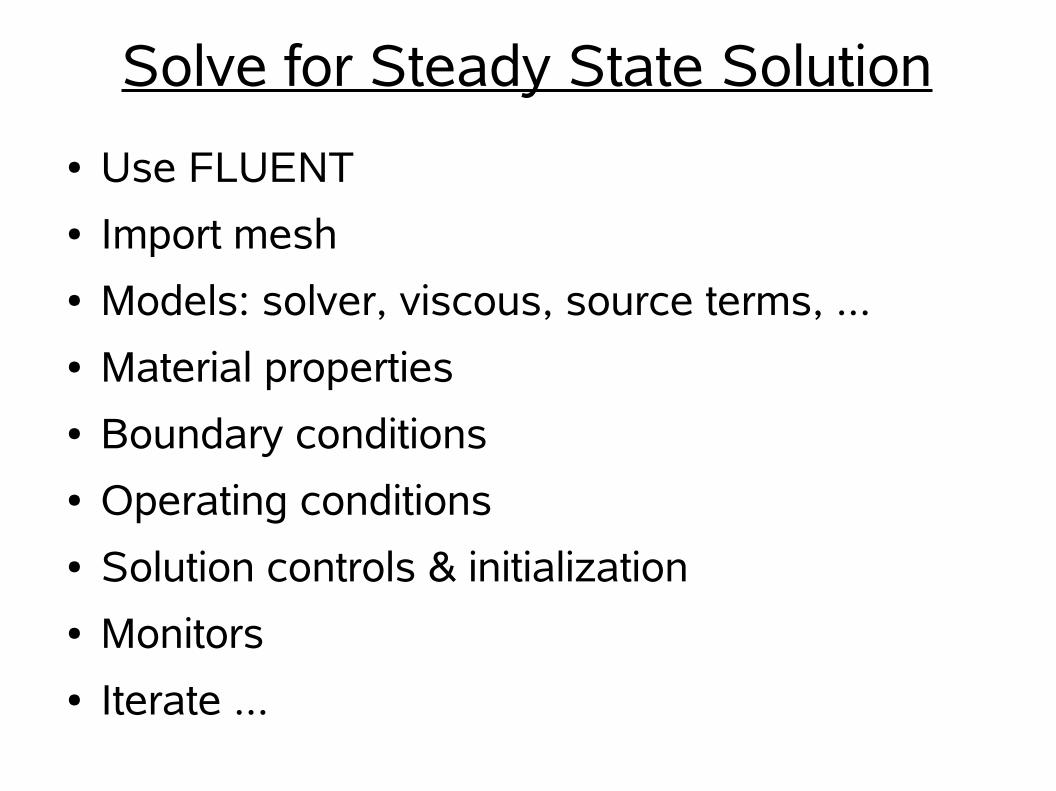
Solve for Steady State Solution
● Use FLUENT● Import mesh● Models: solver, viscous, source terms, ...● Material properties● Boundary conditions● Operating conditions● Solution controls & initialization● Monitors● Iterate ...

Setup FLUENT● Use “step” project directory
– Contains file: step.msh
● Set environment: module load fluent– Only need to do once per shell
– Can put “module load ...” in file: .bashrc
● Run FLUENT for 2D simulations
fluent 2D
● Import mesh from file step.msh
File -> Read -> Case
● Check mesh: Grid -> Check
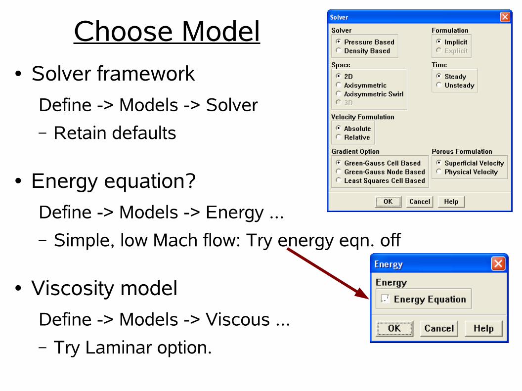
Choose Model● Solver framework
Define -> Models -> Solver
– Retain defaults
● Energy equation?
Define -> Models -> Energy ...
– Simple, low Mach flow: Try energy eqn. off
● Viscosity model
Define -> Models -> Viscous ...
– Try Laminar option.

Materials & Boundaries
● Select fluid
Define -> Materials ...
– Can select from Database
– Can define your own
– Will keep default: air● Dynamic Viscosity: 1.7894e-05 [kg/m-s]
● Boundaries: Define -> Bounary Conditions– Select Inlet (Velocity Inlet) & Set...
– Set Velocity Magnitude: 0.002435 m/s (Re ~ 500)
– Retain default settings for outlet (Pressure Outlet)
– Retain defaults for all other boundaries (Wall)

Operating Conditions & Solver Controls● Set operating conditions
Define -> Operating Conditions ...
– Retain defaults
● NOTE: panel entry fields adapt to model chosen.
Set solver controlsSolve -> Controls -> Solution● Discretization: Momentum: 2nd order
Upwind● Retain other defaults

Initialization & Monitors● Initialize flow on mesh
Solve -> Initialize -> Initialize ...
– Compute From: inlet
– Init
● Solution convergence monitors
Solve -> Monitors -> Residual ...
– Select “Plot” under Options
– Increase Storage & Plotting iterations to 10000
– Keep Continuity, X-, & Y-velocity monitors

Iterative Solution to Steady State● Iterate
Solver -> Iterate ...
– Set # of iterations to 1000
– Iterate
● Laminar: unrealistic– Low res. mesh
– Numerical Diff.
– Need Turb. Visc.
● Save settings & data
File -> Write -> Case & Data ...
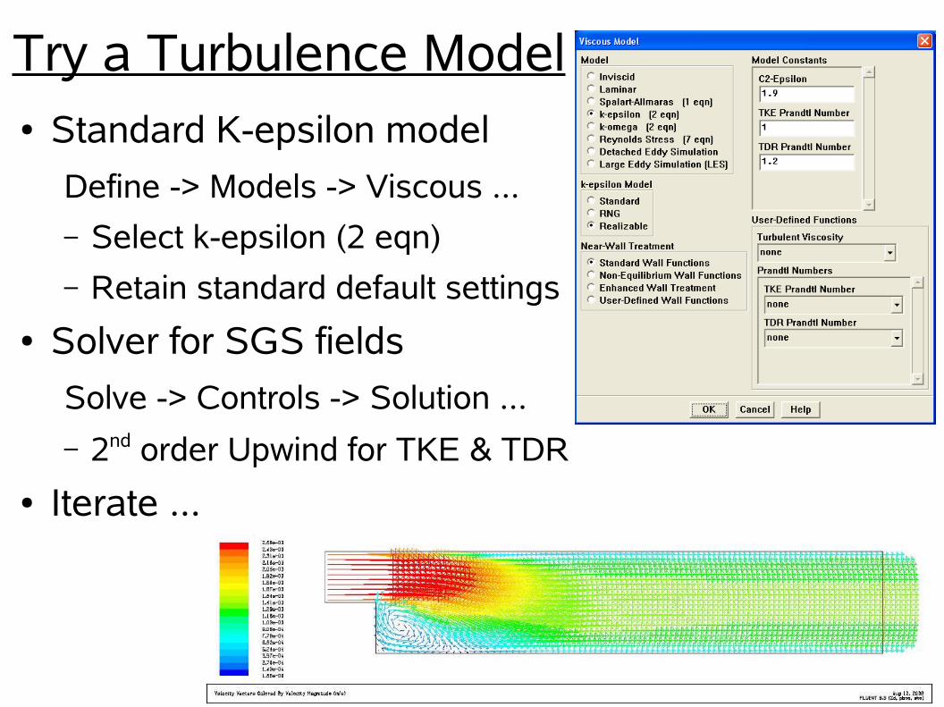
Try a Turbulence Model● Standard K-epsilon model
Define -> Models -> Viscous ...
– Select k-epsilon (2 eqn)
– Retain standard default settings
● Solver for SGS fields
Solve -> Controls -> Solution ...
– 2nd order Upwind for TKE & TDR
● Iterate ...

Examine Flow● Vector fields● Contours● Particle paths● XY plots along lines or edges● Quantitative reports● Compare results from different models● Hard copy output
File -> Hardcopy ...
– I've used: JPEG & Color
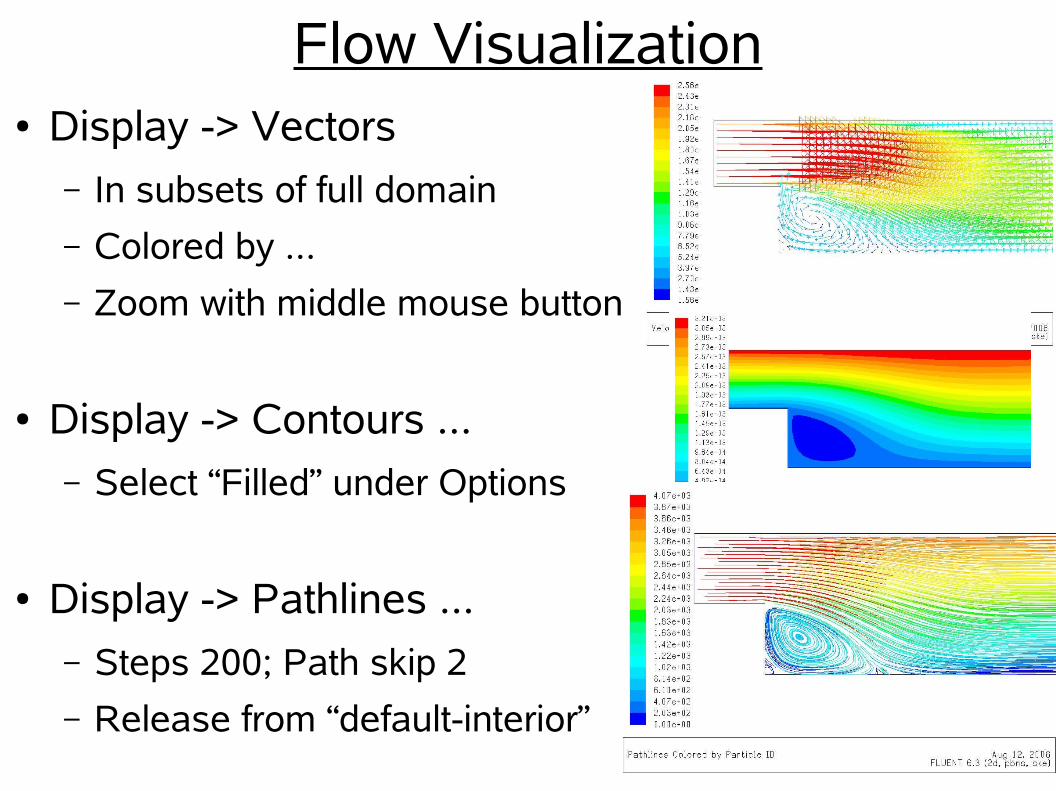
Flow Visualization● Display -> Vectors
– In subsets of full domain
– Colored by ...
– Zoom with middle mouse button
● Display -> Contours ...– Select “Filled” under Options
● Display -> Pathlines ...– Steps 200; Path skip 2
– Release from “default-interior”
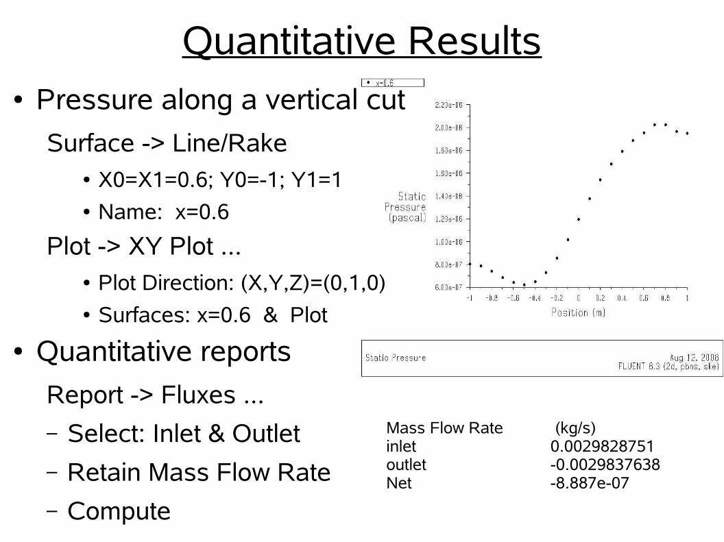
Quantitative Results● Pressure along a vertical cut
Surface -> Line/Rake● X0=X1=0.6; Y0=-1; Y1=1● Name: x=0.6
Plot -> XY Plot ...● Plot Direction: (X,Y,Z)=(0,1,0)● Surfaces: x=0.6 & Plot
● Quantitative reports
Report -> Fluxes ...
– Select: Inlet & Outlet
– Retain Mass Flow Rate
– Compute
Mass Flow Rate (kg/s)inlet 0.0029828751outlet -0.0029837638Net -8.887e-07
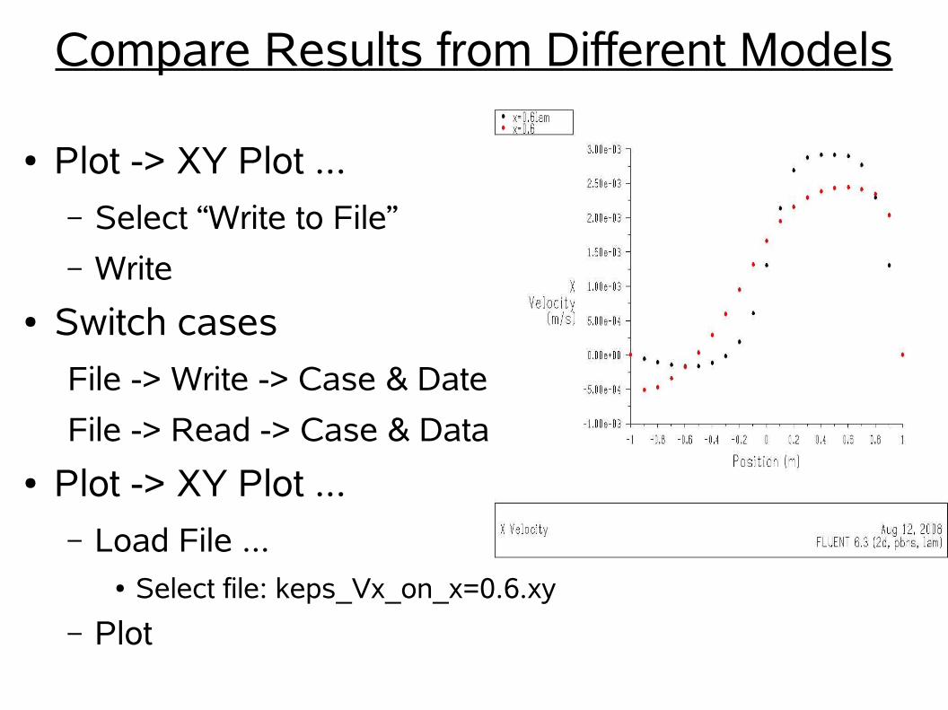
Compare Results from Different Models
● Plot -> XY Plot ...– Select “Write to File”
– Write
● Switch cases
File -> Write -> Case & Date
File -> Read -> Case & Data
● Plot -> XY Plot ...– Load File ...
● Select file: keps_Vx_on_x=0.6.xy
– Plot

Adapt/Refine Mesh
● Reason: test & improve accuracy● Refinement based on your choice of
– Gradients
– Residual errors
– Domain
● Adapt -> Region– X=[-1,10]; y=[-1,1]
– Adapt● doubles mesh
● Solver -> Iterate ...

Comparison of Vx from 3 Models

User Resources at MSI● User Guide & tutorials on the WEB:
– GAMBIT: http://wwwr.msi.umn.edu/gambit/index.htm
– FLUENT: http://wwwr.msi.umn.edu/fluent/index.htm
● MSI User Support– Email: [email protected]
– Phone: 612–626–0802 (8:30am – 5pm)
● MSI web portals & Forums– Still in planning stages
– Will be under MSI web site http://www.msi.umn.edu

Proposed:MSI Forum on Fluid Dynamics/Continuum Mech.
● Interdisciplinary & interdepartmental– Theory, Experiment, Computation
– Facilitate access to local resources & opportunities
– Share knowhow
– Address questions & concerns with MSI resources
– Brainstorm projects leveraged by MSI resources
● Still in planning stages– Forums will be user driven
– Your input is crucial
– Email: [email protected]