1

Mass Spec Data Post-Processing SoftwareClinProTools

Presenter:

Email:Phone:

Help:

Wayne Xu, Ph.D

Supercomputing Institutewxu@msi.umn.edu

(612) 624-1447help@msi.umn.edu (612) 626-0802

Aug. 24,Thur. 2006

Outline• Introduction• ClinProTools functions• Models in ClinProTools• Demo ClinProTools

– Data preparation workflow– Peak statistics workflow– Generate models workflow– Classify samples workflow

2

Introduction

Mass Data Acquisition & Post Processing

Samples

Instruments

Acquisition Software

Data

FlexControl

Bruker’s mass spectrometer

Methods & parameters

post data analysis

MALDI-TOF protocol_1

ClinProTools, ….

ClinProt kits

Spectra data

Center for Mass Spectrometry and Proteomics, UMN,

“Proteomics Workshop”, 5-6 times / year

3

Post Data Analysis Software in Supercomputing Institute

• Post data analysis software: Analyze data that comes off from the mass spec instruments

– Analyst QS– BioAnalysis– ClinProTools– Mascot– Sequest– Peaks Online– Pro ID– Pro QuanT– Pro TS Data– Scaffold

Sample Preparation• Sample types

– For peptide mass fingerprint– For tandem mass (ms/ms)– For quantitative Traq labeling – For intact mass (biological fluids)

• Biological fluids preparation (blood serum, blood plasma,..):

– Highly concentrated components, similar mass to charge (m/z) ratio, may result in overlapping peaks.

– A selective enrichment of specific proteins according to their biological, chemical or physical properties can improve spectra quality significantly.

– Bruker’s enrichment/prefraction magnetic microbead system with different functionalized surfaces are provided as different profiling kits (ClinProt Kits) and each kit contains a detailed protocol for sample preparation (optimized on blood serum).

– Mass analysis reproducibility is significantly depending on reproducibility of sample preparation

4

Post Processing• Visualization

– trace, virtual gel, contour, stacked view

• Data preparation – baseline subtraction, calibration, normalization– m/z, peak intensity, peak area

Data mining– Peak statistics– Database search– Building predictive model– ....

ClinProTools Functions

5

ClinProTools Functions• Main:

– Combine intuitive visualization and multiple mathematical algorithms to generate pattern recognition models

• Use:– Detect intact protein differential levels between cases

and controls in order to discover biomarkers topredict or diagnose diseases

Features• Visualization:

– averaged spectra, compared spectra, and single spectrum with intuitive visualization features such as trace, virtual gel, contour and stacked views

• Data normalization:– processing parameters for baseline substraction, peak

definition, calibration, normalization• Data mining:

– Averages and compares peaks from different spectra– Generates and validates pattern recognition models using

different sophisticated mathematical and bioinformaticalgorithms

• Biomarkers:– Highlights the locations of the biomarkers and allows users

to visually inspect individual spectrum to verify their results• Results:

– Stores the detailed results for each analysis

6

Models in ClinProTools

Models• Models are built on training data (known

cases and known controls), and then used to classify new spectra samples

• ClinProTools supports three kinds of algorithms for generating classification models

– Genetic Algorithm (GA)– Support Vector Machine Algorithm (SVM)– QuickClassifier Algorithm (QC)

7

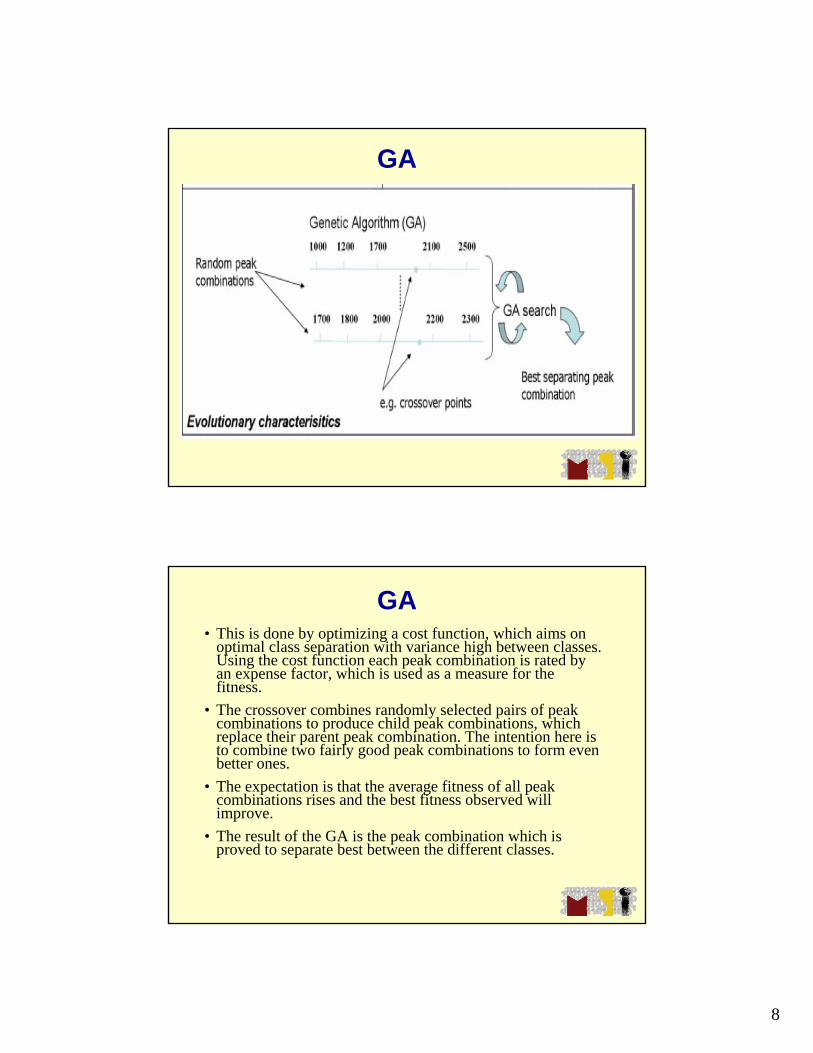
Genetic algorithm (GA)

• GA which mimics evolution in nature, is used to select the peak combinations which are most relevant for separation.

GA• The idea of evolution in which the fittest individuals have the highest chances

of survival.

• Select combinations of peaks, which perform best in separating the classes under consideration.

• Pattern determination is used to identify an optimal set of peaks, which gives the best separating model determined upon the model generation spectra used and validated on test spectra or by a cross validation procedure.

• A brute force approach would not work: A systematic trial of all combinations would take far too long because the number of possible combinations is extremely large. For 1000 given peaks and a desired com-bination of just 3 peaks, you get 1,000*999*998 = 997,002,000 sets of peaks! There-fore, we need more sophisticated ways to do it.

• The advantage of the GA is that it needs much less computational time than the brute force approach while still yielding good results.

8

GA

GA• This is done by optimizing a cost function, which aims on

optimal class separation with variance high between classes. Using the cost function each peak combination is rated by an expense factor, which is used as a measure for the fitness.

• The crossover combines randomly selected pairs of peak combinations to produce child peak combinations, which replace their parent peak combination. The intention here is to combine two fairly good peak combinations to form even better ones.

• The expectation is that the average fitness of all peak combinations rises and the best fitness observed will improve.

• The result of the GA is the peak combination which is proved to separate best between the different classes.

9

Support Vector Machine Algorithm (SVM)

• SVM is motivated from statistical learning theory and is at first used to determine separation planes between the different data classes. Upon the obtained planes, a peak ranking can be calculated in a second step.

Support Vector Machine Algorithm (SVM)

10

VSM• A peak ranking is derived from the obtained hyperplane solution. The procedure is iterated until for each class a classifier (class vs rest) is obtained.

• Upon the obtained SVM model the best number of peaks is determined by a clustering in the subspace taken from the k best peaks and the (best) solution is stored as the final model.

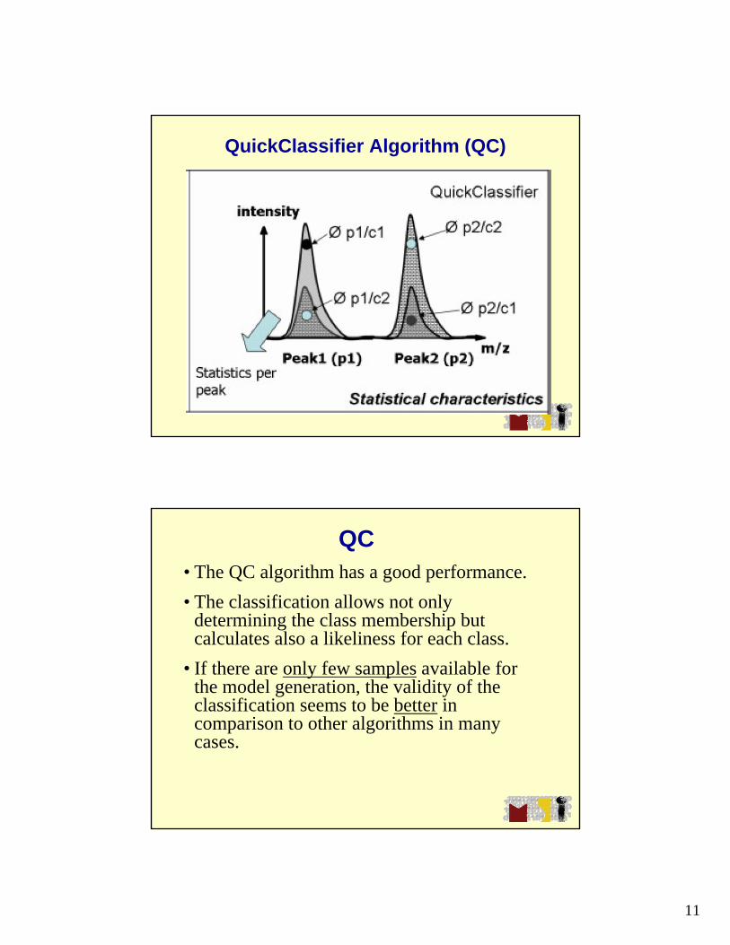
QuickClassifier Algorithm (QC)• a univariate sorting algorithm. The class

averages of the peak areas are stored in the model together with some statistical data like the p-values at certain peak positions.

• For classification, the peak areas are sorted per peak and a weighted average over all peaks is calculated.

11

QuickClassifier Algorithm (QC)

QC• The QC algorithm has a good performance. • The classification allows not only

determining the class membership but calculates also a likeliness for each class.

• If there are only few samples available for the model generation, the validity of the classification seems to be better in comparison to other algorithms in many cases.

12

QC• At first for each peak position, the class averages of

the peak areas are calculated.• These averages are stored in the model together

with the weights determined from the statistical tests.

• For classification at each peak position the reciprocal difference of the peak area and the class averages are calculated and normalized.

• In the next step over all peak positions from these values weighted averages for the classes are calculated.

• To determine the class member ship these weighted averages are compared.

Cross Validation• Evaluate the performance of a classifier for a given data set

and under a given parameterization. • Different methods (random, K-fold, leave one to split a

given set of data into a model generation and a test set. • The model generation set is used to determine a model by

use of the chosen classifier. The test set is than used to evaluate the obtained model and to determine the prediction capability.

• This procedure is repeated multiple times and the absolute prediction capabilities are accumulated

• The cross validation is calculated only if at least 20 not excluded spectra over all groups are available.

13

External Validation•Load new spectra data for each class that was not used in the class generation, but is known to be that class

Getting Start with ClinProTools

14

Data Preparation workflow• Includes:

– Baseline subtraction– Normalization of spectra– Recalibration of specta– Total average of spectrum calculation– Peak area detection on the total average spectra– Area calculation of each peak– Normalization of peak area (GA, SVM only)

• Result:– A collection of peak area for each spectra

• Implemented in settings and automatically started:– Settings spectra preparation– Settings peak calculation

Peak Statistic workflow•Includes:

–Spectra recalibration–Average spectra calculation–Peak picking–Area calculation–Peak statistic

15

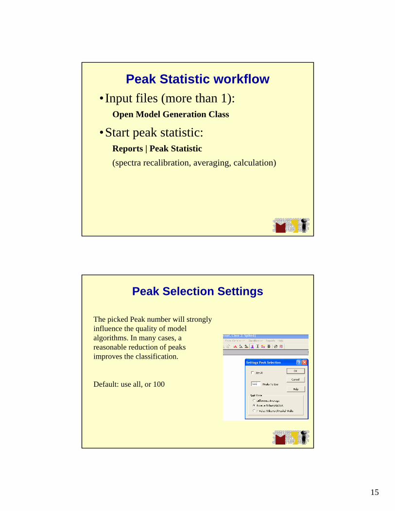
Peak Statistic workflow•Input files (more than 1):

Open Model Generation Class

•Start peak statistic:Reports | Peak Statistic(spectra recalibration, averaging, calculation)

Peak Selection Settings

The picked Peak number will strongly influence the quality of model algorithms. In many cases, a reasonable reduction of peaks improves the classification.

Default: use all, or 100

16

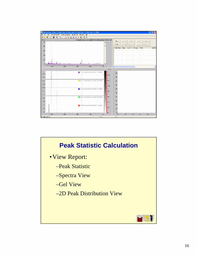
Peak Statistic Calculation

Peak Statistic Calculation

•View Report:–Peak Statistic–Spectra View–Gel View–2D Peak Distribution View

17

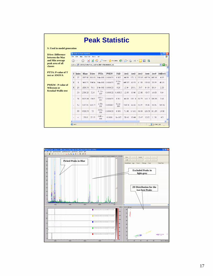
Peak StatisticS: Used in model generation

DAve: Difference between the Max and Min average peak area of all classes

PTTA: P-value of T test or ANOVA

PWKW: P-value of Wilcoxon or Kruskal-Wallis test

Peak Statistic CalculationPicked Peaks in Blue

Excluded Peaks in light-grey

2D Distribution for the two best Peaks

18

Model Generation workflow

• Includes:– Spectra recalibration– Average spectra calculation– Peak calculation– Model generation

Model Generation workflow• Input files:

File | Opene Model generation Class (normal vsspiked)

• Select models:Model Generation | New ModelUse default settings

• Generate models:Model Generation | Calculate

• Save models:Model Generation | Save Model As

19

View Models• :

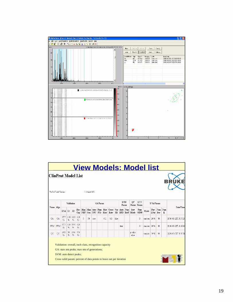
View Models: Model list

•Model list:

Validation: overall, each class, recognition capacity

GA: max nm peaks; max nm of generations;

SVM: auto detect peaks;

Cross valid param: percent of data points to leave out per iteration

20

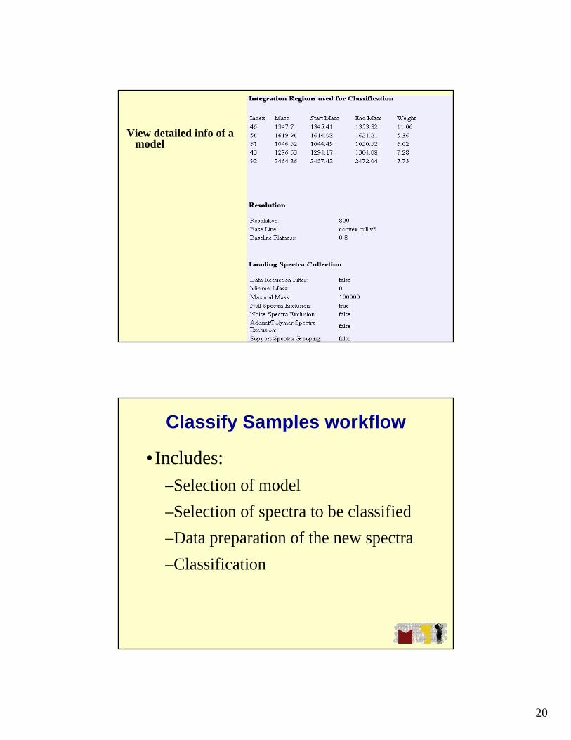
View detailed info of a model

Classify Samples workflow

•Includes:–Selection of model–Selection of spectra to be classified–Data preparation of the new spectra–Classification

21

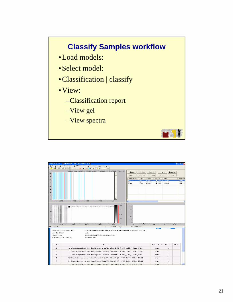
Classify Samples workflow•Load models:•Select model:•Classification | classify•View:

–Classification report–View gel–View spectra

View Classify Samples