introduction to elk stack - mindtree whitepaper.pdf · introduction to elk stack g oal of this...
TRANSCRIPT
1
INTRODUCTION TO ELK STACK
Goal of this document: A simple yet effective document for folks who want to learn basics of ELK (Elasticsearch, Logstash and Kibana) without any prior knowledge.
Introduction: Elasticsearch is a search engine that stores data in the form of documents (JSON). Each document can be compared to a row in a RDBMS. Like any other database, the ‘insert’, ‘delete’, ‘update’ and ‘retrieve’ operations can be done in Elasticsearch. However, as the name suggests, the main purpose or the primary objective of Elasticsearch lies in its very powerful search capacity. It is built on open source project Apache Lucene.
Kibana is a visualization tool that analyzes and visually represents the data from Elasticsearch in the form of chart, graph and many other formats.
Logstash is a data processing pipeline that pulls in data in parallel from various sources, parses, and transforms it into a convenient format for fast and easy analysis, and finally sends it to Elasticsearch or any other destination of choice.
Pre-requisite: Basic understanding of JSON.
Note: This document is based on Elasticsearch version 6.
Instructions are based on Windows OS.
Installation of the ELK stack:
Java (JDK) should be installed on the machine before the ELK stack is installed.
JDK can be downloaded from the site:
https://www.oracle.com/technetwork/java/javase/downloads/index.html
Once Java is installed, download the ELK stack from the Elasticsearch site:
https://www.elastic.co/downloads
Once downloaded, follow the installation steps mentioned in the above link.
To start Elasticsearch, Logstash and Kibana, go to the bin folder of the installation directory and run the respective bat files, “elasticsearch”, “logstash” and “kibana”.
Logstash takes the configuration file as a parameter to get started as shown in example below:
logstash –f config.conf
Examples of configuration file could be found in https://www.elastic.co/guide/en/logstash/5.3/config-examples.html
Note: the path of an input file within the configuration file should contain forward slash even if it’s in Windows. e.g. path => “D:/ELK/data/logs”
Before starting Kibana, update the “kibana.yml” that is in the config folder of your Kibana installation directory, with an entry for the Elasticsearch url, to point to its instance.
E.g. elasticsearch.url: “http://localhost:9200”.
In essence, Elasticsearch should be started first, followed by Kibana.
2
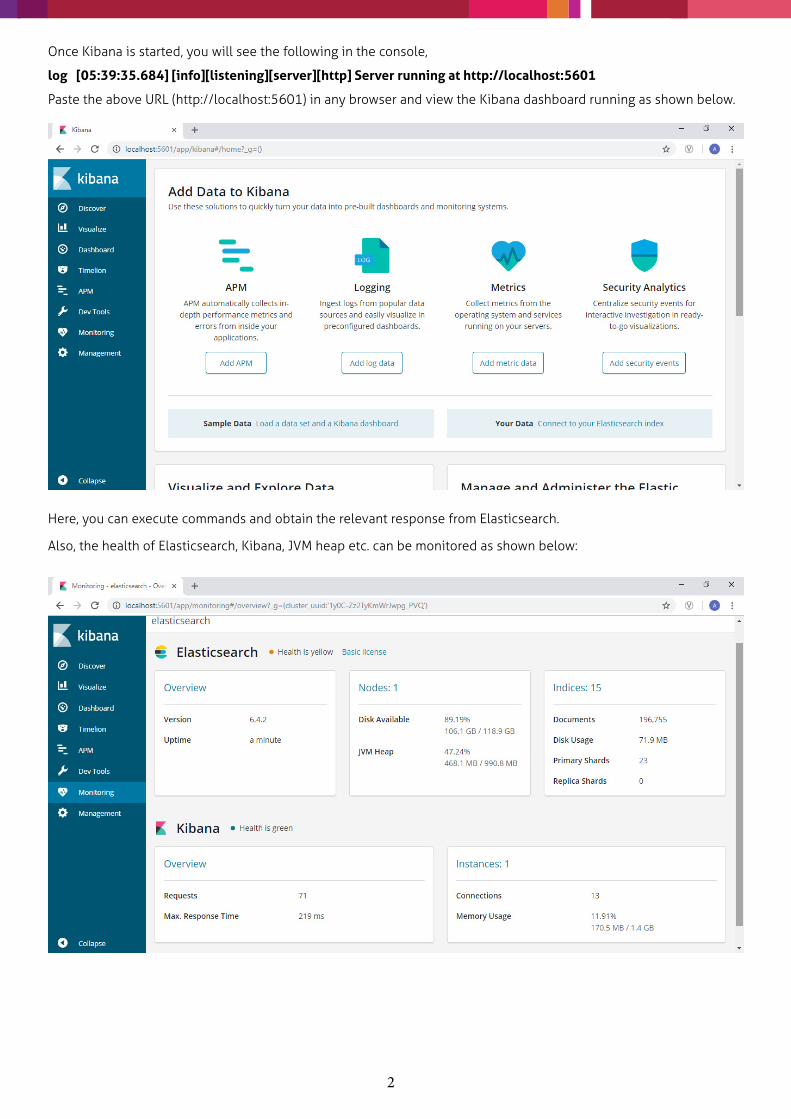
Once Kibana is started, you will see the following in the console,
log [05:39:35.684] [info][listening][server][http] Server running at http://localhost:5601
Paste the above URL (http://localhost:5601) in any browser and view the Kibana dashboard running as shown below.
Here, you can execute commands and obtain the relevant response from Elasticsearch.
Also, the health of Elasticsearch, Kibana, JVM heap etc. can be monitored as shown below:
3
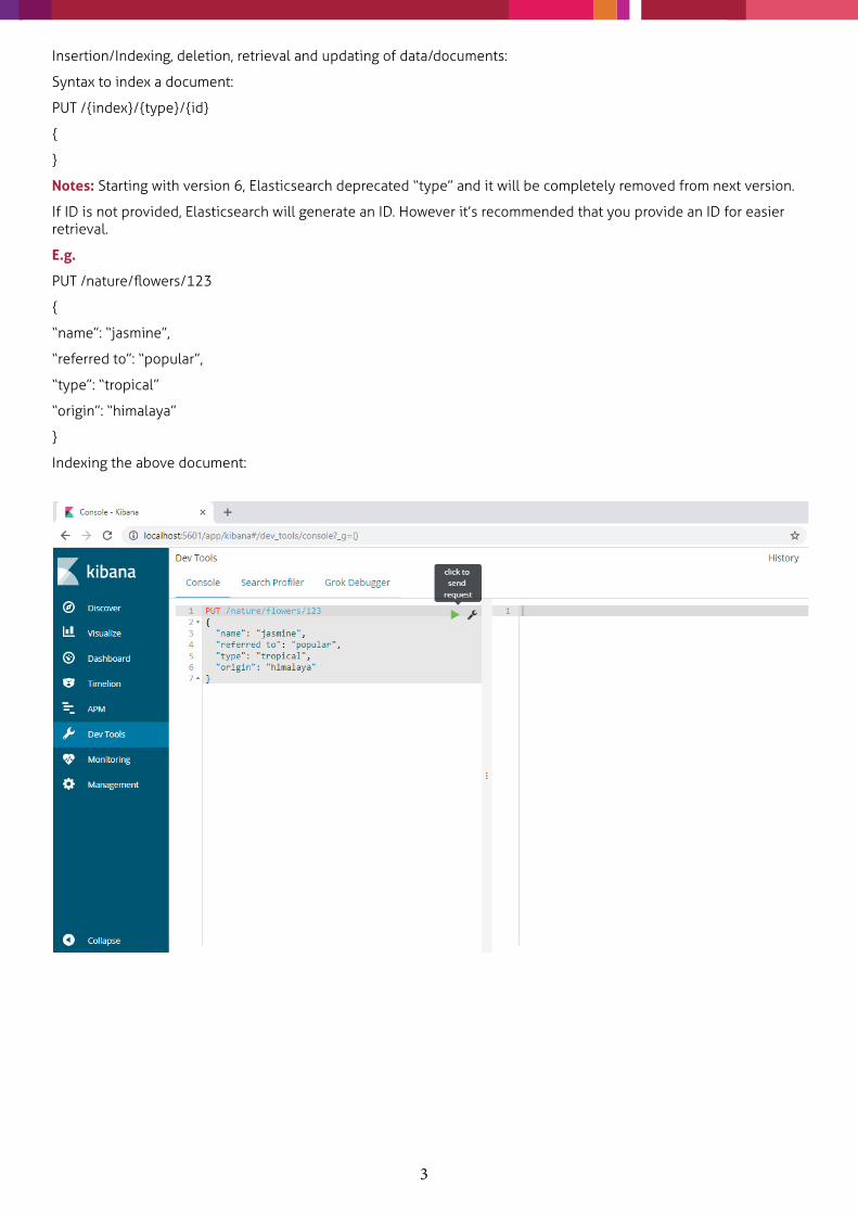
Insertion/Indexing, deletion, retrieval and updating of data/documents:
Syntax to index a document:
PUT /{index}/{type}/{id}
{
}
Notes: Starting with version 6, Elasticsearch deprecated “type” and it will be completely removed from next version.
If ID is not provided, Elasticsearch will generate an ID. However it’s recommended that you provide an ID for easier retrieval.
E.g.
PUT /nature/flowers/123
{
“name”: “jasmine”,
“referred to”: “popular”,
“type”: “tropical”
“origin”: “himalaya”
}
Indexing the above document:
4
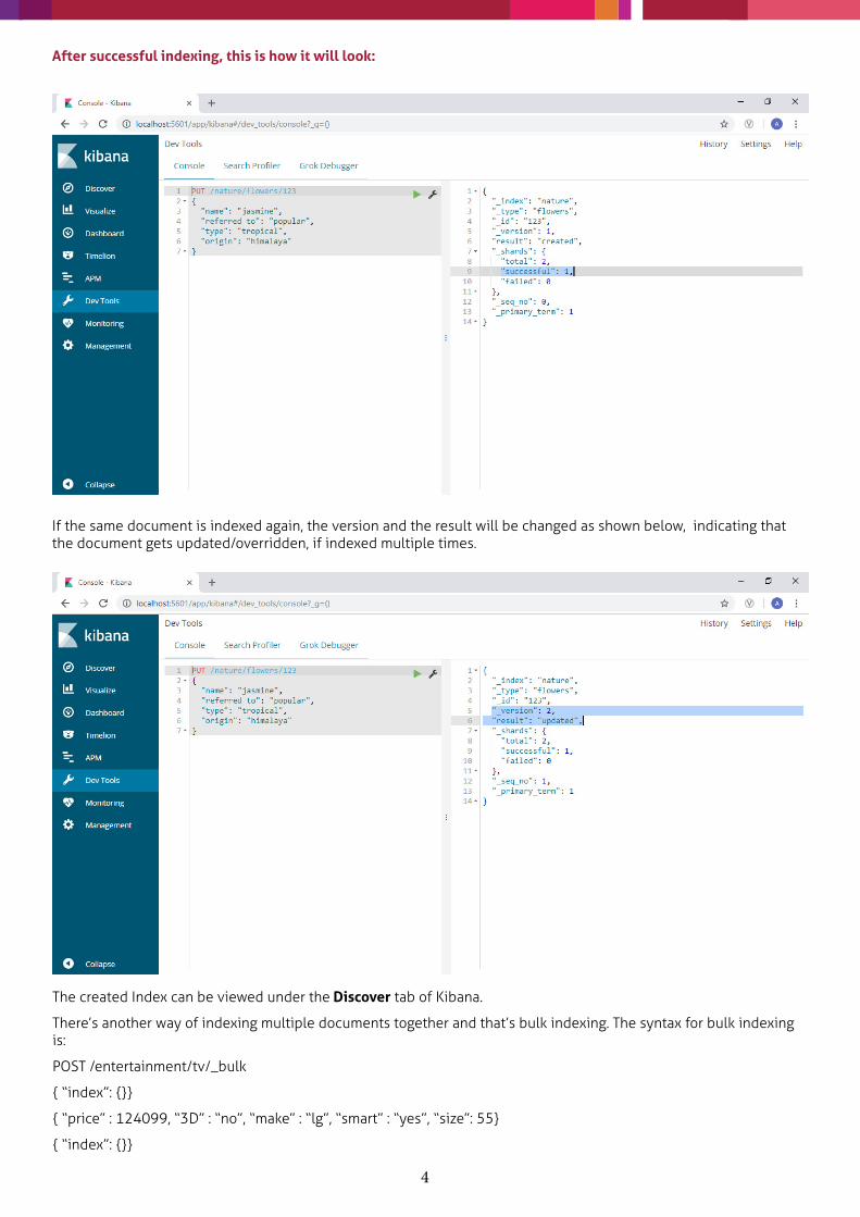
After successful indexing, this is how it will look:
If the same document is indexed again, the version and the result will be changed as shown below, indicating that the document gets updated/overridden, if indexed multiple times.
The created Index can be viewed under the Discover tab of Kibana.
There’s another way of indexing multiple documents together and that’s bulk indexing. The syntax for bulk indexing is:
POST /entertainment/tv/_bulk
{ “index”: {}}
{ “price” : 124099, “3D” : “no”, “make” : “lg”, “smart” : “yes”, “size”: 55}
{ “index”: {}}
5
{ “price” : 120900, “3D” : “yes”, “make” : “samsung”, “smart” : “yes”, “size”: 55}
{ “index”: {}}
{ “price” : 199800, “3D” : “yes”, “make” : “sony”, “smart” : “yes”, “size”: 55}
{ “index”: {}}
{ “price” : 89999, “3D” : “no”, “make” : “haier”, “smart” : “yes”, “size”: 55}
{ “index”: {}}
{ “price” : 141333, “3D” : “no”, “make” : “panasonic”, “smart” : “no”, “size”: 65}
In the above scenario, the ID will be auto-generated.
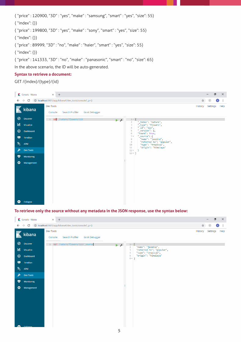
Syntax to retrieve a document:
GET /{index}/{type}/{id}
To retrieve only the source without any metadata in the JSON response, use the syntax below:
6
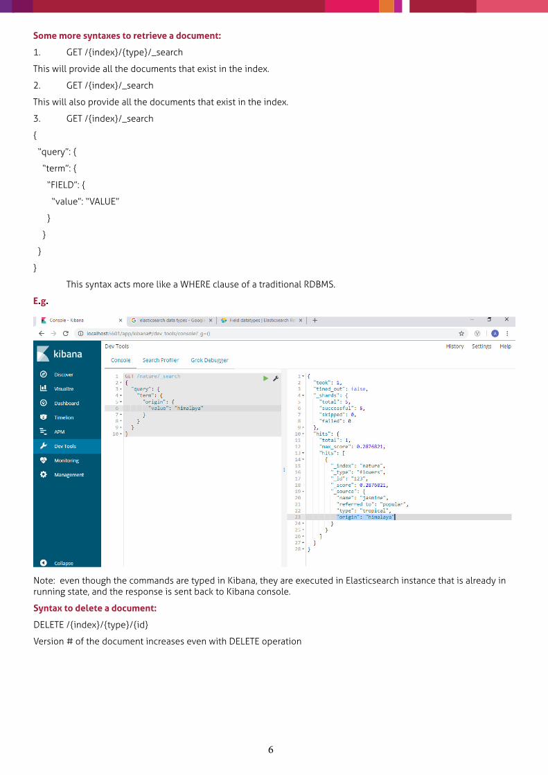
Some more syntaxes to retrieve a document:
1. GET /{index}/{type}/_search
This will provide all the documents that exist in the index.
2. GET /{index}/_search
This will also provide all the documents that exist in the index.
3. GET /{index}/_search
{
“query”: {
“term”: {
“FIELD”: {
“value”: “VALUE”
}
}
}
}
This syntax acts more like a WHERE clause of a traditional RDBMS.
E.g.
Note: even though the commands are typed in Kibana, they are executed in Elasticsearch instance that is already in running state, and the response is sent back to Kibana console.
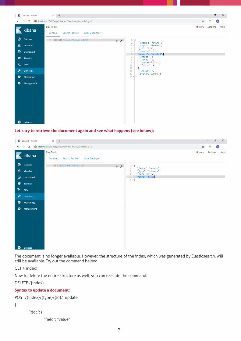
Syntax to delete a document:
DELETE /{index}/{type}/{id}
Version # of the document increases even with DELETE operation
7
Let’s try to retrieve the document again and see what happens (see below):
The document is no longer available. However, the structure of the index, which was generated by Elasticsearch, will still be available. Try out the command below:
GET /{index}
Now to delete the entire structure as well, you can execute the command:
DELETE /{index}
Syntax to update a document:
POST /{index}/{type}/{id}/_update
{
“doc”: {
“field”: “value”
8
}
}
However, POST and PUT work same way. At the backend, it re-indexes the complete document.
Shards and Replicas
Documents in an index can be split across multiple nodes (Elasticsearch clusters) and physically stored in a disc - in something called Shards. For example, if we have 500 documents and have 5 nodes cluster of Elasticsearch, we can split 100 documents in each of the 5 shards. However, it’s the Elasticsearch that combines the data from different shards and responds back when queried which means the request can be made to any node. Also, it makes sure the data in shards are in complete sync with its replicas in the case of operations like indexing, deletion etc.
Shards allow parallel operations across nodes and thus improve performance.
Elasticsearch allows the creation of copies of the shards to ensure a failover mechanism in a distributed environment. These copies are called Replicas. It’s very important to make a note here that the original shard and its replica are never on the same node, otherwise it would defeat the purpose of having replica if that node goes down for any reason.
Querying exact value and full text
Querying exact value is like extracting data with a WHERE clause in a SQL statement. On the contrary, the full text is textual data, like the body of an email, which is hardly used as an exact match to retrieve data. Rather, specific text is searched within that textual data. Also, it’s expected that the search is intelligent enough to understand the intention behind the search.
For example:
1. If someone searches for “run”, it should return documents containing “running”, “runner” etc.
2. If the user searches for any abbreviated word, it should return documents containing the exact match of that word and also the elaborated text.
3. If the user searches for a word, and the same word appears in sentence case, CAPS or lower case in multiple documents, then all those documents should be returned.
To achieve this level of intelligence, Elasticsearch analyzes the text and builds inverted index.
Elasticsearch comes with many built-in analyzers as well as a custom analyzer to satisfy specific needs.
What does Analyzer do?
Analyzer converts the text into tokens and adds those to inverted index to facilitate the search. If the entire text is simply tokenized, the volumes would be very high with many unnecessary tokens. So, to reduce the volume into meaningful tokens, Elasticsearch analyzer typically uses filters like:
1. Removing common stop words like “The”, “was”, “and”.
2. Lowercasing the words.
3. Stemming the words, i.e., reducing words like “running” and “runner” to “run”.
4. Using synonyms
To do this conversion, it analyzes the text with built-in or custom analyzer based on the configuration.
Note: The Analyzer is applied on the document being indexed. Specifically, it’s applied on a particular field when the Analyzer is enabled for that specific field.
How the index structure and analyzer are configured?
It’s not recommended that Elasticsearch define your index structure. Instead, you should define the structure to impose more restriction/security as shown below.
PUT /nature
{
“settings”: {
“number_of_shards”: 2,
“number_of_replicas”: 2
},
“mappings”: {

9
“flowers”: {
“properties”:{
“name”: {
“type”: “text”
},
“easily_available”: {
“type”: “boolean”
},
“type”: {
“type”: “text”
},
“date_of_entry”:{
“type”: “date”
},
“no_of_petals”:{
“type”: “integer”
},
“description”: {
“type”: “text”,
“analyzer”: “standard”
}
}
}
}
}
10
Note: With the above configuration of the index structure, any additional field apart from those mentioned in the mapping section can also be indexed, and Elasticsearch will add them to the mapping section for that extra field. To restrict that, the parameter “dynamic” should be added in the mapping section as follows:
GET /nature/_mapping/flowers
{
“dynamic”: “false”
}
This will not allow the additional field to be indexed, hence it will not be searchable. But at the same time, it will not throw any error even though it appears on the _source field.
Again, if you need it to throw an error in case any additional field is attempted to be indexed, then you need to set it to “strict”. The error thrown in this case would be as follows: “strict_dynamic_mapping_exception”.
Note: Index structure/mapping cannot be changed once created. If you need to change it, then another index structure with modified mapping should be created and all the documents from the existing index must be copied using Reindex API as shown below:
POST _reindex
{
“source”: {
“index”: “<source index name>”
},
“dest”: {
“index”: “<new index name>”
}
}
Querying in Elasticsearch
DSL: Domain specific language or DSL is the language that Elasticsearch uses to write the queries. It has two contexts, Query context and Filtering context.
Query Context
Relevancy score: The more number of times a specific term being searched is found in a document, the more relevant the document, and it will therefore be positioned at the top of the search results.
Syntax to retrieve all the documents of an Index:
GET /{index}/_search
{
“query”: {
“match_all”: {}
}
}
Check the relevancy score here, it will be “1” for all the documents.
Note that max of 10 records are shown in the Kibana console. If more than 10 documents are to be displayed then a parameter called “size” is to be added in the search criteria like:
GET /{index}/_search
{
“size”: 20,
“query”: {
“match_all”: {}
}
}
11
The documents can be sorted as shown below:
GET /{index}/_search
{
“query”: {
“match_all”: {}
}
, “sort”: [
{
“FIELD”: {
“order”: <”desc” or “asc”>
}
}
]
}
Syntax to retrieve the documents of an index based on a specific term:
GET /{index}/_search
{
“query”: {
“match”: {
“FIELD”: “VALUE”
}
}
}
Syntax to retrieve the documents of an index based on a multiple terms (like AND condition in SQL):
GET /{index}/_search
{
“query”: {
“bool”: {
“must”: [
{
“match”: {
“FIELD”: “TEXT”
}
},
{
“match”: {
“FIELD”: “TEXT”
}
}
]
}
}
}
12
Similar to “must”, we have the “must_not” condition which acts like “NOT EQUAL TO” in SQL.
“Should” is like “NICE TO HAVE” in the result of that query. However, this condition can be forcefully included in the result with a clause “minimum_should_match” - and this should be equal to an integer. This means, if we have multiple conditions inside a “should” block, and if we have <“minimum_should_match”: 1>, then any one of those multiple conditions should match.
There’s another aspect of multi search. Here, a specific term can be searched in multiple fields, using the syntax below:
GET /{index}/_search
{
“query”: {
“multi_match”: {
“query”: “”,
“fields”: []
}
}
}
Note: The “fields” above is an array where multiple fields can be accommodated. The query would return, if it matches any of the fields. However, the more it matches, the higher the relevancy score.
There are many other types of queries that Elasticsearch offers. These can be found under the url: https://www.elastic.co/guide/en/elasticsearch/reference/current/query-dsl.html
Filter Context
Filter context differs from Query context in the following ways:
1. Filtering context does not return relevancy score while Query context returns the result along with th relevancy score.
2. Filter context is faster than Query context.
So, it’s better to use the Filtering context if relevancy score is not something you are looking for.
Syntax to retrieve documents using Filtering context:
GET /{index}/_search
{
“query”: {
“bool”: {
“filter”: {
“bool”: {
“must”:[
{“match”: {“FIELD”: “VALUE”}}
]
}
}
}
}
}
The above will not provide any relevancy score, it would be 0(zero) for all the documents as shown below (check the highlighted “max_score”):

13
However, Query criteria can be added outside the Filtering context and the resultant JSON of that criteria ONLY will contain the relevancy score as shown below (check the highlighted “max_score”). Any other result which is not yielded by the criteria mentioned outside the Filtering context will still have a score of 0(zero):
Aggregation
It refers to the summarized data out of a search query. The main intention behind the aggregation theory is analyzing the data to get some insights into something, say, a business.
Example: Suppose an electronic store stores data in Elasticsearch for all the TV units in their stock and now they want to figure out how many 55 inch TVs there are, and out of those TVs, what’s the maximum, minimum and average price for each brand. To get this data, aggregate functions are used as shown below:
GET /entertainment/tv/_search
{
“query”: {
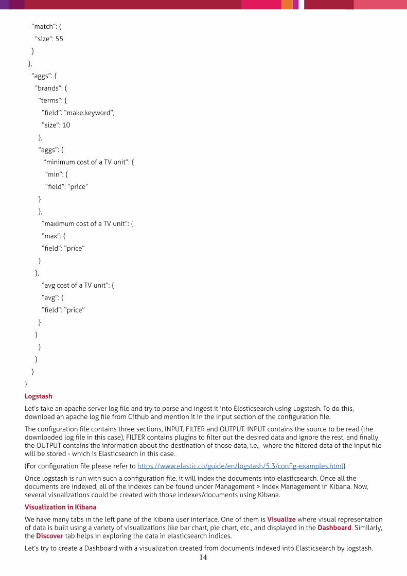
14
“match”: {
“size”: 55
}
},
“aggs”: {
“brands”: {
“terms”: {
“field”: “make.keyword”,
“size”: 10
},
“aggs”: {
“minimum cost of a TV unit”: {
“min”: {
“field”: “price”
}
},
“maximum cost of a TV unit”: {
“max”: {
“field”: “price”
}
},
“avg cost of a TV unit”: {
“avg”: {
“field”: “price”
}
}
}
}
}
}
Logstash
Let’s take an apache server log file and try to parse and ingest it into Elasticsearch using Logstash. To do this, download an apache log file from Github and mention it in the Input section of the configuration file.
The configuration file contains three sections, INPUT, FILTER and OUTPUT. INPUT contains the source to be read (the downloaded log file in this case), FILTER contains plugins to filter out the desired data and ignore the rest, and finally the OUTPUT contains the information about the destination of those data, i.e., where the filtered data of the input file will be stored - which is Elasticsearch in this case.
(For configuration file please refer to https://www.elastic.co/guide/en/logstash/5.3/config-examples.html).
Once logstash is run with such a configuration file, it will index the documents into elasticsearch. Once all the documents are indexed, all of the indexes can be found under Management > Index Management in Kibana. Now, several visualizations could be created with those indexes/documents using Kibana.
Visualization in Kibana
We have many tabs in the left pane of the Kibana user interface. One of them is Visualize where visual representation of data is built using a variety of visualizations like bar chart, pie chart, etc., and displayed in the Dashboard. Similarly, the Discover tab helps in exploring the data in elasticsearch indices.
Let’s try to create a Dashboard with a visualization created from documents indexed into Elasticsearch by logstash.

15
Go to Management > Index Patterns. Look for an index pattern, add a Time Filter field, and then create the index pattern.
Next, go to Visualization > select a Visualization type (e.g. Pie chart) followed by index pattern created above.
Now, select Count as the metrics, and under Buckets > Split Slices, select Aggregation as the Terms, and choose Continent as the Field. Finally, hit the play button. This will give you a pie chart with the document count based on the continent (by default it will provide five in the descending order).
Now go to Dashboard > Add, the visualization created above > Save.
Multiple visualizations such as the above can be added under a single Dashboard.