Introduction to DSGE modelling

Nicola Viegi

University of Pretoria

Dynamic

Stochastic

General Equilibrium

Dynamic

tt-1 t+1

expectations

Stochastic

Impulses

Propagation

Fluctuations

Firms

General equilibrium

Households

Monetary

authority

Households

Maximise present discounted value of expected

utility from now until infinite future, subject to

budget constraint

Households characterised by

utility maximisationconsumption smoothing

Households

+

+

+=

+11

1)

1(')('

t

tt

i

tCUE

tCU

πβ

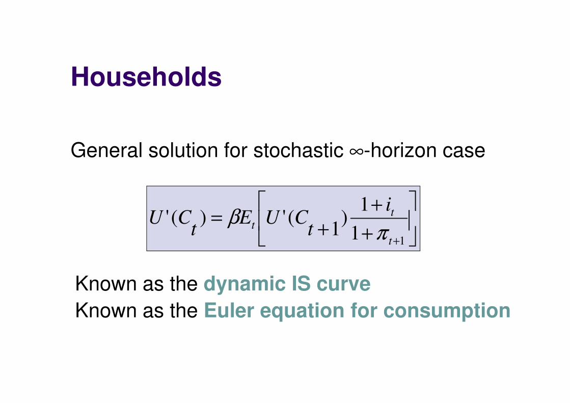
General solution for stochastic ∞-horizon case

Known as the dynamic IS curve

Known as the Euler equation for consumption

Households - intuition

+

+

+=

+11

1)

1(')('

t

tt

i

tCUE

tCU

πβ

it↑ → U’(Ct)↑ → Ct↓ Higher interest rates reduce consumption

Etπt+1↑ → U’(Ct)↓ → Ct ↑ Higher expected future

inflation increases

consumption

Firms

Maximise present discounted value of expected profit from now until infinite future, subject to demand curve, nominal price rigidity and labour supply curve.

Firms characterised by profit maximisationsubject to nominal price rigidity

Nominal price rigidity

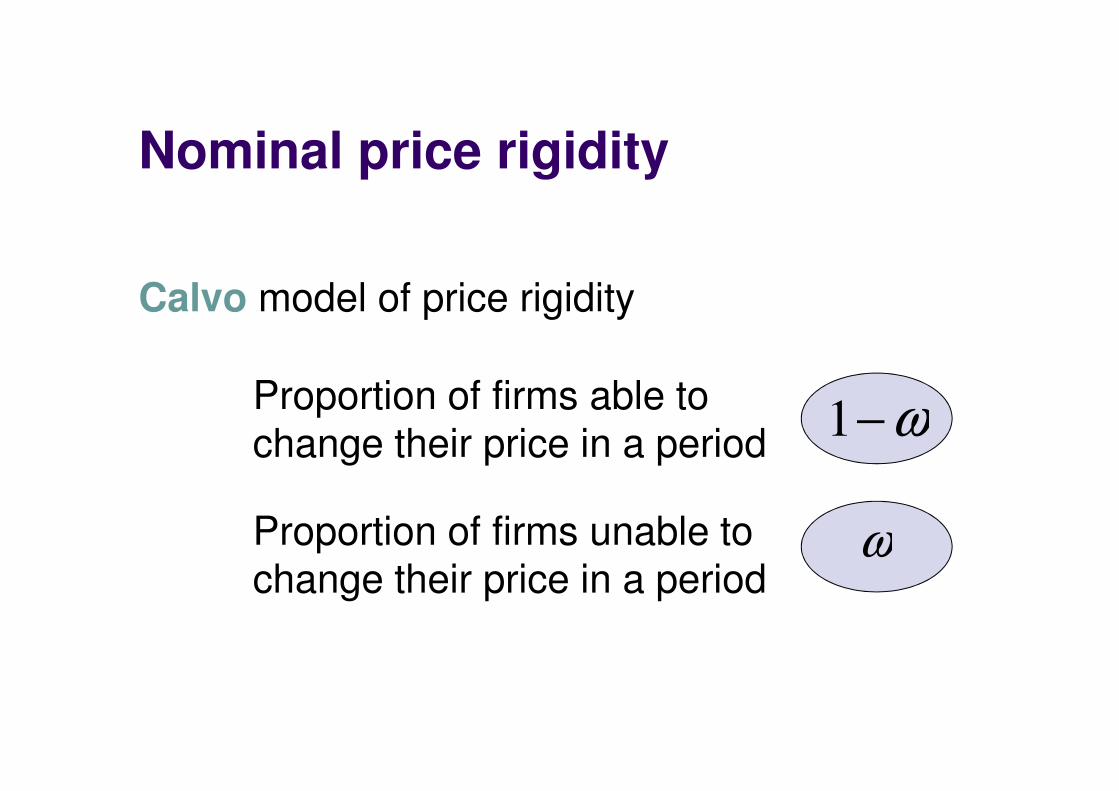
Calvo model of price rigidity

ωProportion of firms unable to

change their price in a period

Proportion of firms able to

change their price in a periodω−1

Firms

)ˆˆ()1)(1(

ˆ1+−

−−= tttt Ex πβπ

βωω

αω

Known as the New Keynesian Phillips curve

Known as the forward-looking Phillips curve

Full solution

Firms - intuition

)ˆˆ()1)(1(

ˆ1+−

−−= tttt Ex πβπ

βωω

αω

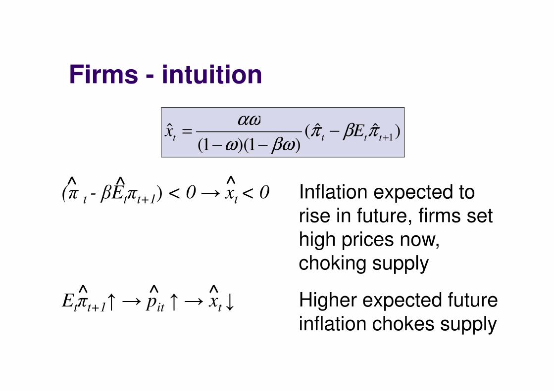
(π t - βEtπt+1) < 0→ xt < 0 Inflation expected to

rise in future, firms set

high prices now,

choking supply

Etπt+1↑ → pit ↑ → xt ↓ Higher expected future

inflation chokes supply

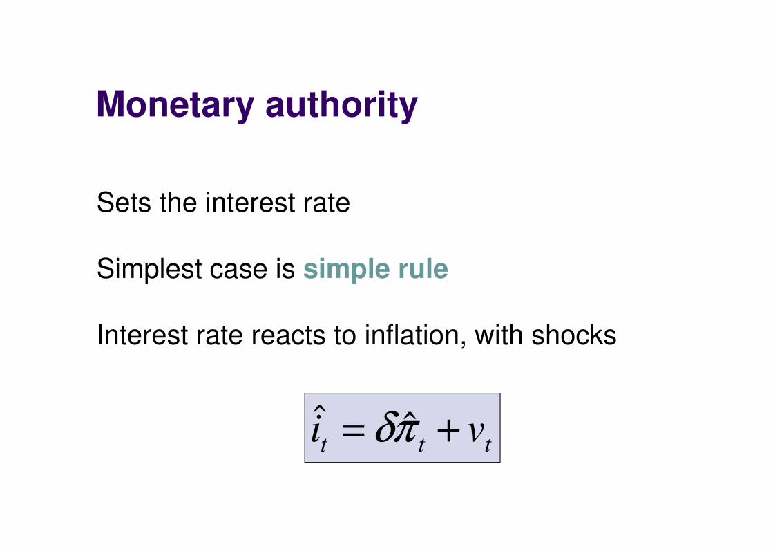
Sets the interest rate

Simplest case is simple rule

Interest rate reacts to inflation, with shocks

Monetary authority

ttt vi += πδ ˆˆ

Firms

Baseline DSGE model

Households

Monetary

authorityttt vi += πδ ˆˆ

+

+

+=

+11

1)

1(')('

t

tt

i

tCUE

tCU

πβ1

ˆ ˆ ˆ( )(1 )(1 )

t t t tx E

αωπ β π

ω βω+= −

− −

Households

Two simplifying assumptions:

CRRA utility functionσ

σ

−=

−

1)(

1

tt

CCU

σ−= tt CCU )('

tt YC =No capital

Firms

Log-linearised DSGE model

Households

Monetary

authorityttt vi += πδ ˆˆ

)ˆˆ(ˆˆ1

1

1 +−

+ −−= tttttt EixEx πσ)ˆˆ()1)(1(

ˆ1+−

−−= tttt Ex ππ

βωω

αω

Calibration

1.5

0.75

0.99

2

α

ω

β

σ

=

=

=

=

Full DSGE model

αω

βωωκ

πδ

κπβπ

πσ

)1)(1(

ˆˆ

ˆˆˆ

)ˆˆ(ˆˆ

1

1

1

1

−−=

+=

+=

−−=

+

+−

+

ttt

tttt

tttttt

vi

xE

EixEx

Alternative representation

tttt

ttttttt

xE

vxExE

πκπβ

σπδσπσ

ˆˆˆ

ˆˆˆˆ

1

11

1

1

1

+−=

++=+

+

−−+

−+

t

t

t

tt

ttv

x

E

xE

+

−=

−−

+

+−

0ˆ

ˆ

1

1

ˆ

ˆ

0

111

1

11 σ

πκ

δσ

πβ

σ

State-space form

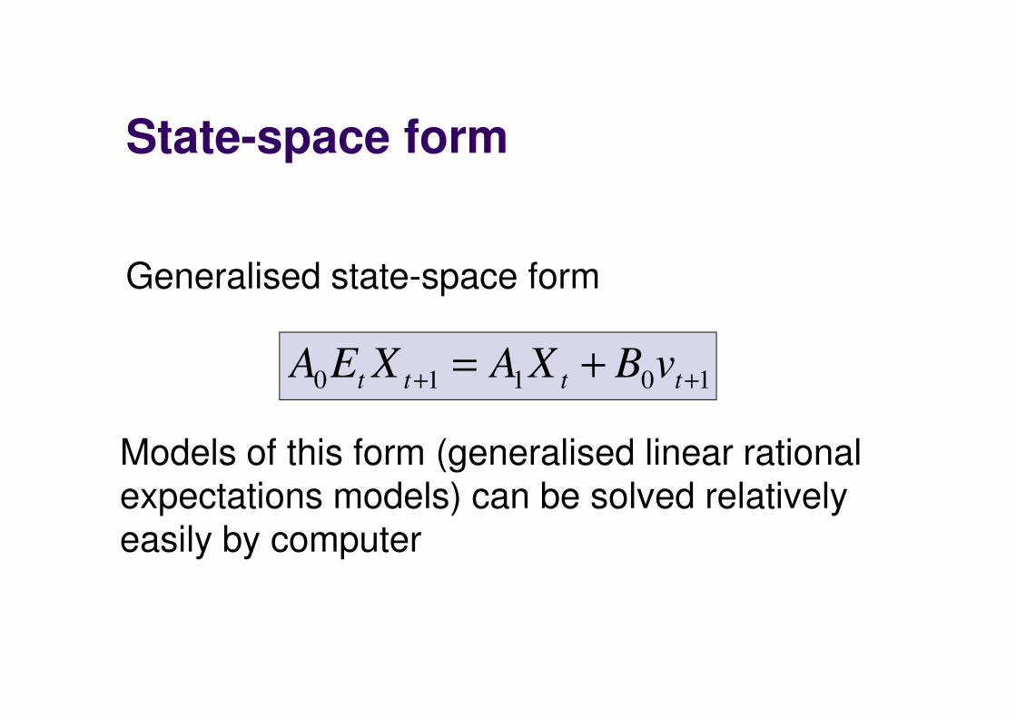
10110 ++ += tttt vBXAXEA

Generalised state-space form

Models of this form (generalised linear rational

expectations models) can be solved relatively

easily by computer

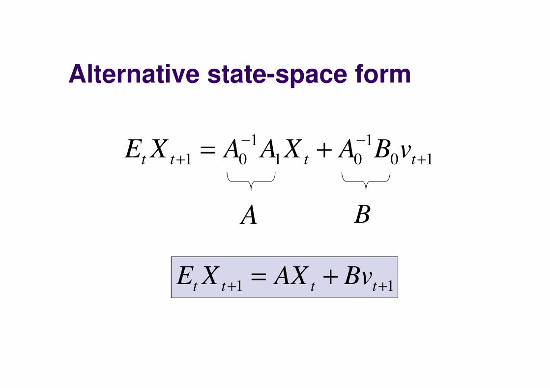
Alternative state-space form

10

1

01

1

01 +−−

+ += tttt vBAXAAXE

11 ++ += tttt BvAXXE

A B

Partitioning of model

1

1

1

+

+

++

=

t

t

t

tt

tBv

y

wA

yE

w

=

t

t

ty

wX

backward-looking variables

predetermined variables

forward-looking variables

control variables

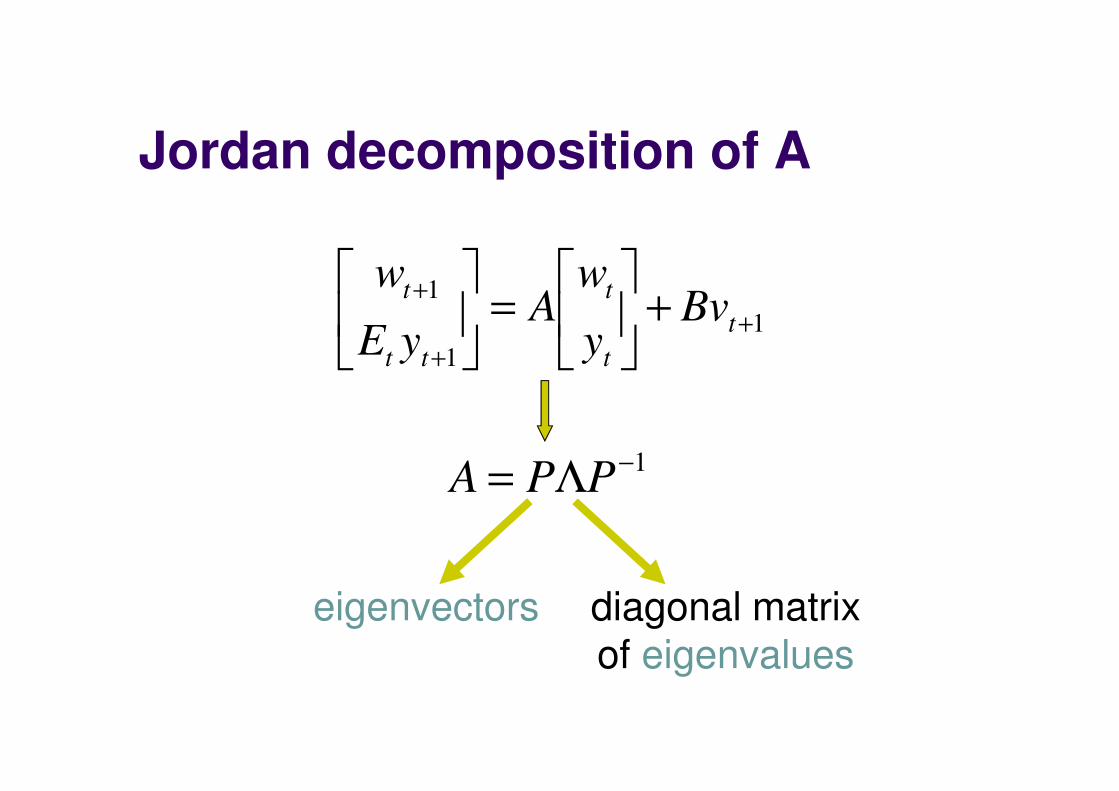
Jordan decomposition of A

1

1

1

+

+

++

=

t

t

t

tt

tBv

y

wA

yE

w

1−Λ= PPA

eigenvectors diagonal matrix

of eigenvalues

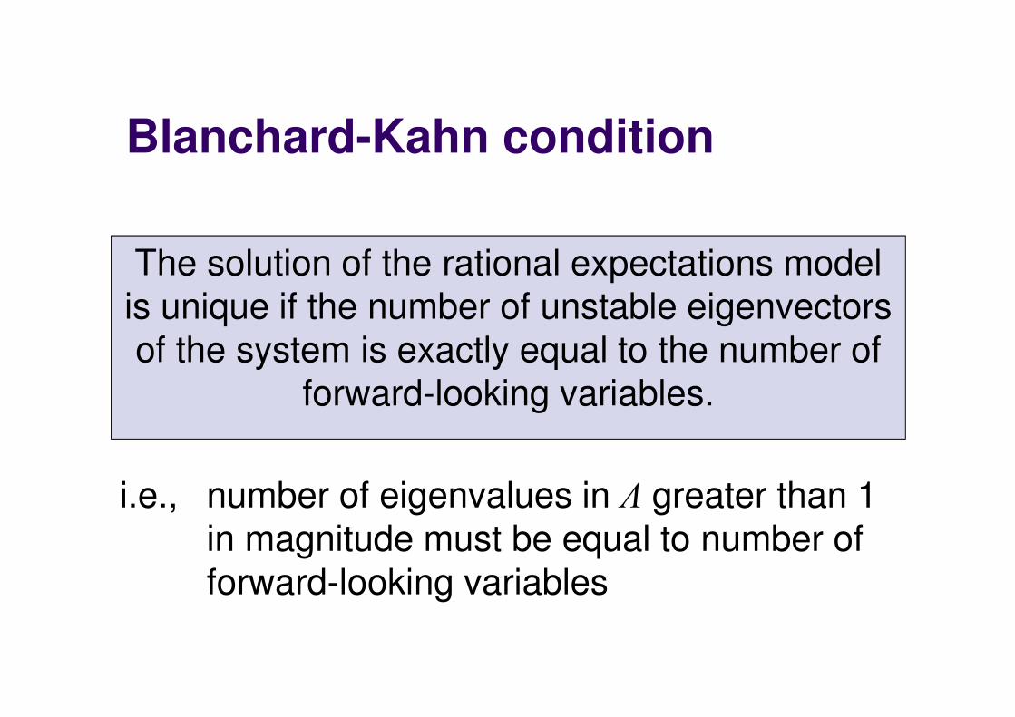
Blanchard-Kahn condition

The solution of the rational expectations model

is unique if the number of unstable eigenvectors

of the system is exactly equal to the number of

forward-looking variables.

i.e., number of eigenvalues in Λ greater than 1

in magnitude must be equal to number of

forward-looking variables

tw

ty

Too many stable roots

0w

multiple solutions

equilibrium path

not unique

need alternative

techniques

tw

ty

Too many unstable roots

0w

no solution

all paths are

explosive

transversality

conditions violated

tw

ty

Blanchard-Kahn satisfied

0w

one solution

equilibrium path

is unique

system has saddle

path stability

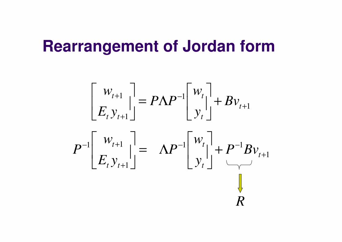
Rearrangement of Jordan form

1

11

1

11

+−−

+

+− +

Λ=

t

t

t

tt

tBvP

y

wP

yE

wP

1

1

1

1

+−

+

++

Λ=

t

t

t

tt

tBv

y

wPP

yE

w

R

Partition of model

Λ

Λ=Λ

2

1

0

0

=−

*

22

*

21

*

12

*

111

PP

PPP

1

1

1

11

+−

+

+− +

Λ=

t

t

t

tt

tRv

y

wP

yE

wP

=

2

1

R

RR

stable

unstable

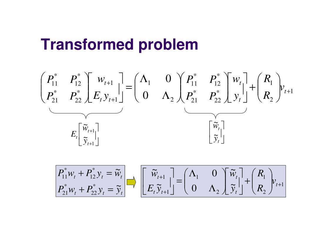
Transformed problem

+

+

1

1

~

~

t

t

ty

wE

t

t

y

w~

~

ttt

ttt

yyPwP

wyPwP

~

~

*

22

*

21

*

12

*

11

=+

=+

1

2

1

*

22

*

21

*

12

*

11

2

1

1

1

*

22

*

21

*

12

*

11

0

0+

+

+

+

Λ

Λ=

t

t

t

tt

tv

R

R

y

w

PP

PP

yE

w

PP

PP

1

2

1

2

1

1

1

~

~

0

0

~

~

+

+

+

+

Λ

Λ=

t

t

t

tt

tv

R

R

y

w

yE

w

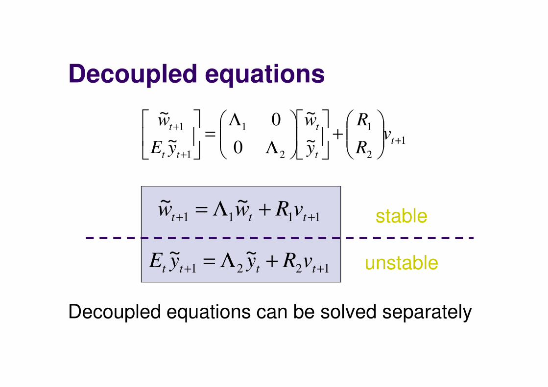
Decoupled equations

1

2

1

2

1

1

1

~

~

0

0

~

~

+

+

+

+

Λ

Λ=

t

t

t

tt

tv

R

R

y

w

yE

w

1111

~~++ +Λ= ttt vRww

1221

~~++ +Λ= tttt vRyyE

Decoupled equations can be solved separately

stable

unstable

Solution strategy

Solve unstable transformed equation ty~

Translate back into

original problem

tw~

t

t

y

w

Solve stable transformed equation

Solution of unstable equation

As , only stable solution is12 >Λ tyt ∀= 0~

0~ *

22

*

21 =+= ttt yPwPy

( ) t

j

jtt yyE ~~2Λ=+

tt wPPy*

21

1*

22

−−=

Solve unstable equation forward to time t+j

Forward-looking (control) variables are function

of backward-looking (predetermined) variables

Solution of stable equation

tt

ttt

wPPy

yPwPw

*

21

1*

22

*

12

*

11

~

−−=

+=

( ) t

j

jtt wwE ~~1Λ=+

tt wPPPPw )(~ *

21

1*

22

*

12

*

11

−−=

Solve stable equation forward to time t+j

As , no problems with instability11

<Λ

Solution of stable equation

11

1*

21

1*

22

*

12

*

11

*

21

1*

22

*

12

*

111

1*

21

1*

22

*

12

*

111

)(

)()(

+−−

−−−+

−+

−Λ−=

t

tt

vRPPPP

wPPPPPPPPw

1111

~~++ +Λ= ttt vRww

tt wPPPPw )(~ *

21

1*

22

*

12

*

11

−−=11

*

21

1*

22

*

12

*

11

~)( ++

− =− tt wwPPPP

Future backward-looking (predetermined)

variables are function of current backward-

looking (predetermined) variables

Full solution

11

1*

21

1*

22

*

12

*

11

*

21

1*

22

*

12

*

111

1*

21

1*

22

*

12

*

111

*

21

1*

22

)(

)()(

+−−

−−−+

−

−+

−Λ−=

−=

t

tt

tt

vRPPPP

wPPPPPPPPw

wPPy

All variables are function of backward-looking

(predetermined) variables: recursive structure

Baseline DSGE model

t

t

t

tt

ttv

x

E

xE

+

−=

−−

+

+−

0ˆ

ˆ

1

1

ˆ

ˆ

0

111

1

11 σ

πκ

δσ

πβ

σ

11 ++ += ttt vv ερ

State space form

To make model more interesting, assume policy shocks vt follow an AR(1) process

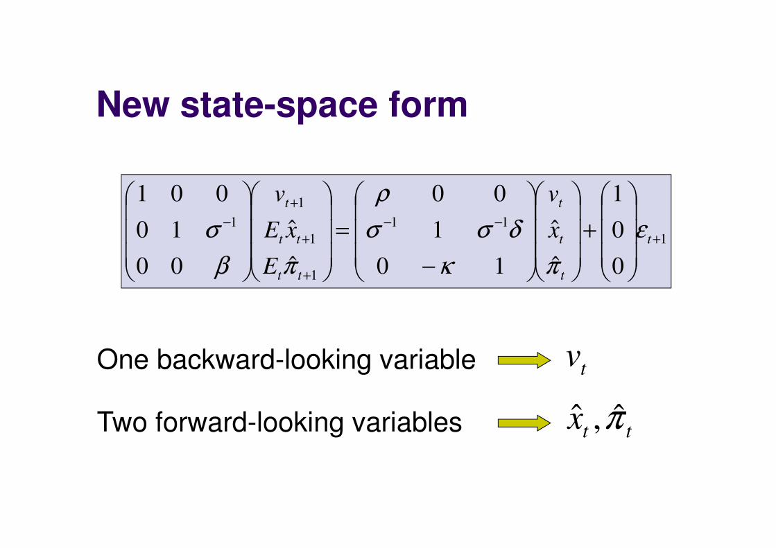
New state-space form

tv

1

11

1

1

1

1

0

0

1

ˆ

ˆ

10

1

00

ˆ

ˆ

00

10

001

+−−

+

+

+

−

+

−

=

t

t

t

t

tt

tt

t

x

v

E

xE

v

ε

πκ

δσσ

ρ

πβ

σ

ttx π̂,ˆ

One backward-looking variable

Two forward-looking variables

Blanchard-Khan conditions

=

=

t

t

t

tt

xy

vw

π̂

ˆ

Require one stable root and two unstable roots

Partition model according to

More complex models

Impulses

Propagation

Fluctuations

Frisch-Slutsky paradigm

Shocks may be correlated

Impulses

Can add extra shocks to the model

ttt

ttttt

ttttttt

vi

uxE

gEixEx

+=

++=

+−−=

+

+−

+

πδ

κπβπ

πσ

ˆˆ

ˆˆˆ

)ˆˆ(ˆˆ

1

1

1

1

+

=

+

+

+

+

+

+

g

t

u

t

v

t

t

t

t

t

t

t

g

u

v

g

u

v

1

1

1

333231

232221

131211

333231

232221

131211

1

1

1

ε

ε

ε

υυυ

υυυ

υυυ

ρρρ

ρρρ

ρρρ

Propagation

Add lags to match dynamics of data

(Del Negro-Schorfeide, Smets-Wouters)

ttxtt vxi ++= ˆˆˆ δπδπTaylor rule

ttt

p

t

p

p

t

ttttttt

xE

EixEh

xh

hx

ˆˆ1

ˆ1

ˆ

)ˆˆ(ˆ1

1ˆ

1ˆ

11

1

1

11

κπβγ

βπ

βγ

γπ

πσ

++

++

=

−−+

++

=

+−

+−

+−

29.01

35.01

≈+

≈+

p

p

h

h

βγ

γ

Simulation possibilities

Stylised facts

Impulse response functions

Forecast error variance decomposition

Optimised Taylor rule

What are best values for parameters in Taylor

rule ?ttxtt vxi ++= ˆˆˆ δπδπ

Introduce an (ad hoc) objective function for policy

)ˆˆˆ(min222

0

titxt

i

iix λλπβ ++∑

∞

=

Brute force approach

Try all possible combinations of Taylor rule

parameters

Check whether Blanchard-Kahn conditions are

satisfied for each combination

For each combination satisfying B-K condition,

simulate and calculate variances

Brute force method

Calculate simulated loss for each combination

Best (optimal) coefficients are those satisfying

B-K conditions and leading to smallest

simulated loss

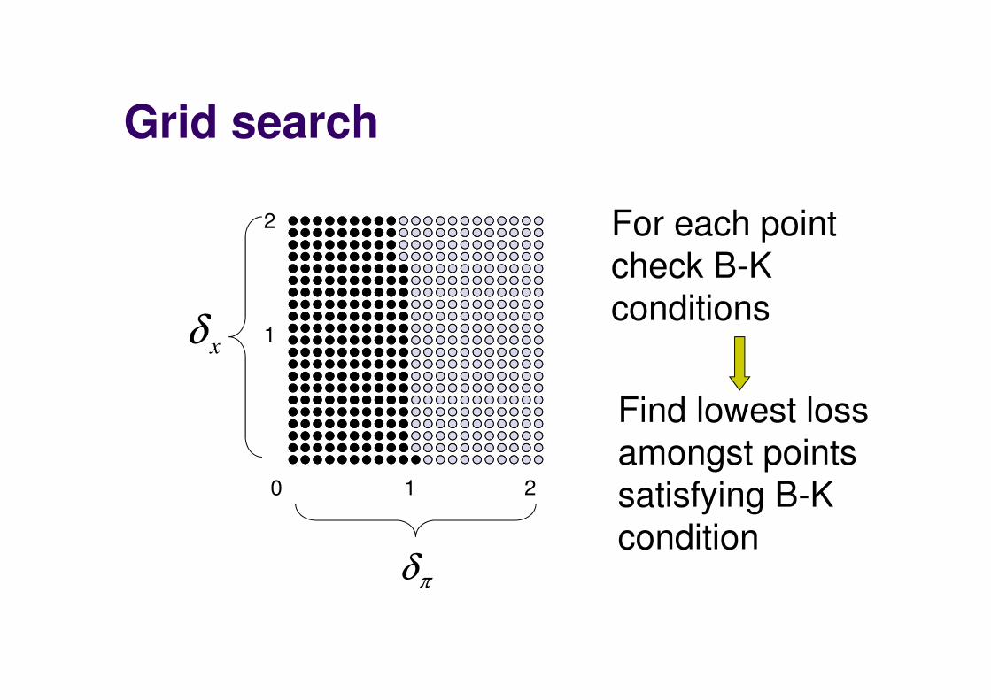
Grid search

πδ

xδ

0 1 2

2

1

For each point

check B-K

conditions

Find lowest loss

amongst points

satisfying B-K

condition