LBNL-59975

Introduction to Commercial Building Control Strategies and Techniques for Demand Response

N. Motegi, M.A. Piette, D.S. Watson, S. Kiliccote, P. Xu Energy Environmental Technologies Division

May 2007

 

 

 

 

 

 

 

 

Introduction to Commercial Building Control Strategies and Techniques for Demand Response 

 

Naoya Motegi Mary Ann Piette David S. Watson  Sila Kiliccote Peng Xu  

Lawrence Berkeley National Laboratory 

MS90R3111 

1 Cyclotron Road 

Berkeley, California 94720 

 

May 22, 2007 

 

This work described in this report was coordinated by the Demand Response Research Center and funded by the California Energy Commission, Public Interest Energy Research Program, under Work for Others Contract No. 500‐03‐026 and by the U.S. Department of Energy under Contract No. DE-AC02-05CH11231. 

 

LBNL Report Number 59975

   

  i

Acknowledgements

The work described  in  this report was coordinated by  the Demand Response Research Center and funded by the California Energy Commission (Energy Commission), Public Interest Energy Research (PIER) Program, under Work for Others Contract No. 500‐03‐026  and by the U.S. Department of Energy under Contract No. DE‐AC02‐05CH11231. 

The authors wish to thank the engineers and staff at each building site.  Special thanks to Ron Hofmann  for his  conceptualization of  this project and ongoing  technical  support.  Thanks  also  to  Laurie  ten  Hope, Mark  Rawson,  and  Dave Michel  at  the  California Energy  Commission.  Finally,  thanks  to  the  Pacific  Gas  and  Electric  Company  who funded the Automated CPP research.    

We  appreciate  the  helpful  comments  provided  by  the  peer  reviewers  of  this  report: Douglas  B.  Nordham  (EnerNOC),  Austen  D’Lima  (San  Diego  Gas  and  Electric Company), Steve Greenberg and Barbara Atkinson (LBNL). 

 

 

 

 

 

 

 

 

 

 

 

 

 

 

 

 

Please cite this report as follows:  

Motegi, N., M.A. Piette, D.S. Watson, S. Kiliccote, P. Xu. 2006. Introduction to Commercial Building  Control  Strategies  and  Techniques  for  Demand  Response.  California  Energy Commission, PIER. LBNL Report Number 59975. 

   

  ii

Preface 

The  Public  Interest  Energy  Research  (PIER)  Program  supports  public  interest  energy research  and  development  that will  help  improve  the  quality  of  life  in California  by bringing environmentally safe, affordable, and reliable energy services and products to the marketplace. 

The  PIER  Program,  managed  by  the  California  Energy  Commission  (Energy Commission), annually awards up to $62 million to conduct the most promising public interest energy research by partnering with Research, Development, and Demonstration (RD&D) organizations, including individuals, businesses, utilities, and public or private research institutions. 

PIER funding efforts are focused on the following six RD&D program areas: 

• Buildings End‐Use Energy Efficiency • Industrial/Agricultural/Water End‐Use Energy Efficiency • Renewable Energy • Environmentally‐Preferred Advanced Generation • Energy‐Related Environmental Research • Energy Systems Integration 

What follows is the final report for the Statewide Auto‐DR Collaboration Project, 500‐03‐026,  conducted  by  Lawrence  Berkeley  National  Laboratory.  The  report  is  entitled “Introduction  to Commercial Building Control Strategies and Techniques  for Demand Response.” This project contributes to the Energy Systems Integration Program. 

For more information on the PIER Program, please visit the Energy Commissionʹs Web site  at:  http://www.energy.ca.gov/research/index.html  or  contact  the  Energy Commissionʹs Publications Unit at 916‐654‐5200.  

   

  iii

Table of Contents 

Executive Summary..................................................................................................................... 1

1. Introduction ......................................................................................................................... 1 1.1. Background and Overview........................................................................................ 1 1.2. Objectives ..................................................................................................................... 1 1.3. Research Scope ............................................................................................................ 1 1.4. Benefits to California .................................................................................................. 3 1.5. Report Organization ................................................................................................... 3 1.6. Building Operation and Energy Management Framework .................................. 4 1.7. Terms and Concepts for DR Strategies .................................................................... 6

2. Demand Response Strategy Overview ......................................................................... 10 2.1. HVAC Systems.......................................................................................................... 10 2.2. Lighting Systems....................................................................................................... 14 2.3. Miscellaneous Equipment........................................................................................ 16 2.4. Non‐Component‐Specific Control Strategies........................................................ 16 2.5. Strategies Used in Case Studies .............................................................................. 16

3. Demand Response Strategy Detail................................................................................ 19 3.1. HVAC Systems.......................................................................................................... 19 3.1.1. Global temperature adjustment...................................................................... 20 3.1.2. Passive thermal mass storage ......................................................................... 25 3.1.3. Duct static pressure decrease.......................................................................... 26 3.1.4. Fan variable frequency drive limit................................................................. 27 3.1.5. Supply air temperature increase .................................................................... 28 3.1.6. Fan quantity reduction .................................................................................... 29 3.1.7. Cooling valve limit ........................................................................................... 30 3.1.8. Chilled water temperature increase............................................................... 31 3.1.9. Chiller demand limit........................................................................................ 32 3.1.10. Chiller quantity reduction............................................................................... 34 3.1.11. Rebound avoidance strategies ........................................................................ 36

3.2. Lighting Systems....................................................................................................... 37 3.2.1. Zone switching ................................................................................................. 37 3.2.2. Luminaire/lamp switching.............................................................................. 38 3.2.3. Stepped dimming ............................................................................................. 41 3.2.4. Continuous dimming....................................................................................... 42

3.3. Miscellaneous Equipment........................................................................................ 43 3.4. Non‐Component‐Specific Strategies ...................................................................... 45 3.4.1. Demand limit strategy ..................................................................................... 45 3.4.2. Price‐level response strategy .......................................................................... 46

4. Implementation of DR Strategies .................................................................................. 47 4.1. DR Strategy Development and Commissioning................................................... 47

   

  iv

4.2. Notification to Occupants ........................................................................................ 50 4.2.1. No notification .................................................................................................. 50 4.2.2. Notification........................................................................................................ 50

4.3. Factors that influence demand savings achievement .......................................... 51

5. Discussion and Conclusions........................................................................................... 55 5.1. Discussion .................................................................................................................. 55 5.2. Conclusions................................................................................................................ 56 5.3. Recommendations..................................................................................................... 57 5.4. Benefits to California ................................................................................................ 57

References ................................................................................................................................... 58

Glossary....................................................................................................................................... 60

Appendix A: DR Strategies for HVAC                  A‐1 Appendix B: Summary of DR Strategies............................................................................. B‐1 Appendix C: Case Study of Advanced Demand Response ............................................. C‐1 

  

   

  v

List of Figures 

Figure 1. Examples of load shapes ............................................................................................. 6 Figure 2. HVAC DR strategy decision tree ............................................................................. 11 Figure 3. Lighting DR strategy decision tree .......................................................................... 15 Figure 4. Frequency of DR strategies....................................................................................... 18 Figure 5. Temperature drift rate allowed under ASHRAE Standard 55 .......................... 218 Figure 6. Zone setpoints deadband.......................................................................................... 22 Figure  7.  Conceptual  diagram  of  demand  savings  for  typical  HVAC‐based  demand 

response strategy ............................................................................................................... 24 Figure 8. Luminaire switching – alternate rows of luminaires ............................................ 39 Figure 9. Luminaire switching – every other luminaire in each row.................................. 39 Figure 10. Lamp switching ‐ middle lamps of three‐lamp fixtures..................................... 40 Figure 11. Lamp switching – lamps in each luminaire ......................................................... 40 Figure 12. Example of price‐level zone setpoint control....................................................... 46 Figure 13. Demand savings intensity by shed strategy (W/ft2)............................................ 51 Figure 14. OAT vs. average demand savings ......................................................................... 52 Figure 15. Whole‐building hourly demand vs. OAT and demand sheds .......................... 54

 

List of Tables 

Table 1. Demand side management terminology and building operations......................... 4 Table 2. Building HVAC types ................................................................................................. 11 Table 3. HVAC demand response strategies .......................................................................... 12 Table 4. DR strategies used in LBNL Auto‐DR studies (fully‐automated) ........................ 17 Table 5. DR strategies used in case studies (manual or semi‐automated) ......................... 18 Table 6. Conditions for global temperature adjustment (GTA)........................................... 20 Table 7. Conditions for passive thermal mass storage .......................................................... 25 Table 8. Conditions for duct static pressure decrease ........................................................... 26 Table 9. Conditions for fan variable frequency drive limit .................................................. 27 Table 10. Conditions for supply air temperature reset ......................................................... 28 Table 11. Conditions for fan quantity reduction .................................................................... 29 Table 12. Conditions for cooling valve limit........................................................................... 30 Table 13. Conditions for chilled water temperature increase .............................................. 31 Table 14. Conditions for chiller demand limit........................................................................ 32 Table 15. Conditions for chiller quantity reduction............................................................... 34 Table 16. Conditions for zone switching................................................................................. 37 Table 17. Conditions for luminaire/lamp switching.............................................................. 38 Table 18. Conditions for stepped dimming ............................................................................ 41 Table 19. Conditions for continuous dimming....................................................................... 42 Table 20. Recommended data collection points ..................................................................... 49 Table 21. Demand savings influence factors........................................................................... 51

   

 vi

Table 22. Statistical significance of OAT vs. demand savings.............................................. 53  

   

 vii

Abstract 

Demand Response  (DR)  is a set of  time‐dependent program activities and  tariffs  that seek to reduce electricity use or shift usage to another time period.  DR provides control systems  that encourage  load  shedding or  load  shifting during  times when  the electric grid  is  near  its  capacity  or  electricity  prices  are  high. DR  helps  to manage  building electricity costs and to improve electric grid reliability. 

This  report  provides  an  introduction  to  commercial  building  control  strategies  and techniques for demand response. Many electric utilities have been exploring the use of critical  peak  pricing  (CPP)  and  other  demand  response  programs  to  help  reduce summer  peaks  in  customer  electric  loads. This  report  responds  to  an  identified  need among building operators for knowledge to use DR strategies in their buildings. These strategies can be implemented using either manual or automated methods.   

The  report  compiles  information  from  field  demonstrations  of  DR  programs  in commercial  buildings.  The  guide  provides  a  framework  for  categorizing  the  control strategies  that  have  been  tested  in  actual  buildings.  The  guide’s  emphasis  is  on characterizing and describing DR control strategies for air‐conditioning and ventilation systems. There is also good coverage of lighting control strategies.  The guide provides some additional introduction to DR strategies for other miscellaneous building end‐use systems and non‐component‐based DR strategies.   

The  core  information  in  this  report  is  based  on  DR  field  tests  in  28  non‐residential buildings, most of which were  in California, and  the  rest of which were  in New York State.  The majority  of  the  participating  buildings were  office  buildings. Most  of  the California buildings participated in fully automated demand response field tests. 

 

  

   

  1

Executive Summary 

Introduction 

Demand Response  (DR)  is a set of  time‐dependent program activities and  tariffs  that seek  to reduce or shift electricity usage  to  improve electric grid reliability and manage electricity  costs.  DR  strategies  provide  control  methodologies  that  enhance  load shedding  or  load  shifting  during  times when  the  electric  grid  is  near  its  capacity  or electricity prices are high. Many electric utilities have been exploring the use of critical peak pricing (CPP) and other demand response programs to help reduce summer peaks in customer electric  loads. Recent evaluations have shown that customers have  limited knowledge of how  to operate  their facilities  to reduce  their electricity costs under CPP (Quantum and Summit Blue 2004).  

Purpose 

The purpose of this report is to provide an introduction to commercial building control strategies and techniques for demand response. While energy efficiency measures have been  widely  understood  by  many  audiences  including  facility  managers,  building owners,  control  contractors,  utility  program managers,  auditors,  and  policy makers, there are not many documents introducing frameworks or guidelines for measures and strategies to participate in demand response programs.  

Commercial buildings have been only minor participants in demand response programs. This  report  is  designed  to  be  an  initial  introduction  to  the  technical  capabilities  of existing building equipment and systems and their ability to provide demand response control strategies. While the focus of the guide is on DR, we have found that the process of developing DR control strategies can also help identify strategies for energy efficiency during daily building operations. 

Project Objectives 

The report is a unique guide that compiles information from actual field demonstrations of DR  programs  in  commercial  buildings.  The  guide  provides  background  technical information necessary  to  identify and enable demand response control strategies.   The guide is intended for use by building professionals including facility managers, building owners, control contractors, building engineers, utility personnel, and auditors. 

Project Outcomes 

The guide provides a  framework  for categorizing  the control strategies  that have been tested in actual buildings. The guide’s emphasis is on characterizing and describing DR control  strategies  for  air‐conditioning  and  ventilation  systems,  plus  lighting  control strategies.   The guide provides some additional  introduction  to DR strategies for other miscellaneous building end‐use systems and non‐component‐based DR strategies. These strategies can be implemented using either manual or automated methods.   

   

  2

The  core  information  in  this  report  is  based  on  DR  field  tests  in  28  non‐residential buildings, most of which were  in California, and  the  rest of which were  in New York State.  The majority  of  the  participating  buildings were  office  buildings. Most  of  the California buildings participated in fully automated demand response field tests. 

Heating,  Ventilating,  and  Air  Conditioning  (HVAC).  HVAC  systems  can  be  an excellent  resource  for  DR  savings  for  the  following  reasons.  First,  HVAC  systems comprise a substantial portion of the electric load in commercial buildings. Second, the “thermal  flywheel”  (thermal  storage)  effect  of  indoor  environments  allows  HVAC systems  to  be  temporarily  unloaded  without  immediate  impact  on  the  building occupants. Third,  it  is  common  for HVAC  systems  to  be  at  least partially  automated with energy management and control systems  (EMCS). To provide reliable, repeatable DR control, it is best to pre‐plan and automate operational modes that will provide DR savings. The use of automation reduces the labor required to implement DR operational modes when they are signaled.   

HVAC‐based DR  strategies  recommended  for  a given  facility vary based  on building type and condition, mechanical equipment, and EMCS. Based on these factors, the best DR  strategies  are  those  that  achieve  the  aforementioned  goals  of meeting  electricity demand‐savings  targets while minimizing  negative  impacts  on  the  occupants  of  the buildings  or  the  processes  that  they  perform.  This  guide  discusses  the  following DR strategies for HVAC systems, which are best suited to achieve these goals: 

• Global Temperature Adjustment of Zones, and 

• Systemic Adjustments to the Air Distribution and/or Cooling Systems. 

It  is  often  difficult  to  estimate  the  demand  savings  achieved  by  HVAC  strategies, because  the  building’s  HVAC  electric  load  is  dynamic  and  sensitive  to  weather conditions,  occupancy,  and  other  factors. However,  previous  research  has  found  that HVAC  demand  as  well  as  demand  savings  tend  to  have  positive  correlation  with outside air temperature (OAT). 

Lighting. DR strategies for lighting can also be effective in reducing peak demand. On a hot summer day when daylight is in abundance, daylit and/or over‐lit buildings are the best  candidates  for  lighting  demand  savings.  Since  lighting  produces  heat,  reducing lighting  levels will also reduce  the cooling  load within  the space  (Sezgen and Koomey 1998).  Lighting  DR  strategies  tend  to  be  simple  and  depend  widely  on  wiring  and controls  infrastructures.  However,  since  lighting  has  safety  implications  and  the strategies  tend  to  be  noticeable,  they  should  be  carried  out  selectively  and  carefully, considering  the  tasks  in  the  space and  ramifications of  reduced  lighting  levels  for  the occupants. 

DR control capability of  lighting systems  is generally determined by the characteristics of  the  lighting  circuit  and  the  control  system.  Following  is  the  list  of  lighting  DR strategies discussed in this guide in increasing order of sophistication: 

• Zone switching 

   

  3

• Fixture switching • Lamp switching • Stepped dimming • Continuous dimming 

Miscellaneous  Equipment.  There  is  also  demand  savings  potential  for  certain  other equipment  in both  commercial and  industrial buildings. Equipment or processes with the demand  saving potentials discussed  in  this  report are  fountain pumps, anti‐sweat heaters,  electric vehicle  chargers,  industrial process  loads,  cold  storage,  and  irrigation water pumps. 

Non‐Component‐Specific  Strategies. Other  effective DR  strategies  focus  on  controls settings  rather  than  on  specific  equipment.  Such  strategies  highlighted  in  this  report include demand limit strategy and signal‐level response strategy. 

Conclusions 

HVAC  systems  can  be  an  excellent  resource  for DR  shed  savings  because;  1) HVAC systems  create  a  substantial  electric  load  in  commercial  buildings,  2)  the  thermal flywheel  effect  of  indoor  environments  allows  HVAC  systems  to  be  temporarily unloaded without immediate impact to the building occupants, and 3) it is common for HVAC systems to be at least partially automated with EMCS systems. 

For HVAC DR strategies, global temperature adjustment of zones is the priority strategy that best achieves the DR goal. In contrast, systemic adjustments to the air distribution and/or cooling systems can be disruptive to occupants.  DR strategies that slowly return the  system  to  normal  condition  (rebound  avoidance)  should  be  considered  to  avoid unwanted demand spikes caused by an immediate increase of cooling load. 

Lighting DR  strategies  tend  to  be  simple  and  provide  constant,  predictable  demand savings. Since  lighting produces heat,  reducing  lighting  levels may  reduce  the cooling load  and/or  increase  the  heating  load  within  the  space.    The  resolution  of  lighting controls tends to be lower than that of HVAC controls.  Also lighting systems are often not  automated with  EMCS.    These  issues  can  be major  obstacles  for  automation  of lighting DR strategies. 

If a DR strategy can be achieved without any reduction in service, the strategy should be considered  as  permanent  energy  efficiency  opportunity  rather  than  a  temporary DR strategy.  That  is,  it  should  be  performed  on  non‐DR  days  as well.    The  process  of commissioning  should  be  applied  to  each  phase  of  DR  control  strategy  application, including  planning,  installation,  and  implementation  to  make  sure  the  goal  of  DR control is achieved. 

Recommendations 

The  information  in  this  report  should  be  disseminated  to  key  personnel  who  are involved  in DR  implementation  including  facility managers, building owners, controls contractors, and auditors. Disseminating  this  information will help provide a common understanding  of DR  control  strategies  and  development  procedures  to  enable  these 

   

  4

strategies. The  report  is not an exhaustive  list of all DR  strategies. Further  research  is needed  to better understand  the peak demand  reduction potential  and  capabilities of these strategies for various building types in different climates and occupancy patterns.  One  specific  technical development needed  is  to  explore  the design  and  operation  of simplified peak electric demand savings estimation methods and tools. Current auditors and  building  engineers  have  widely  varying  methods  to  estimate  peak  demand reductions for various strategies. 

Benefits to California 

This  guide  is  based  primarily  on  case  studies  in  California  and  is  intended  to  help streamline  the  DR  control  strategy  implementation  process  and  increase  successful participation  in  DR  programs  in  California.    Peak  demand  reduction  and  demand response are key parts of the state’s energy policies. 

   

  1

1. Introduction

1.1. Background and Overview

Demand Response  (DR)  is a set of  time‐dependent program activities and  tariffs  that seek  to reduce or shift electricity usage  to  improve electric grid reliability and manage electricity  costs.  DR  strategies  provide  control  methodologies  that  enhance  load shedding  or  load  shifting  during  times when  the  electric  grid  is  near  its  capacity  or electricity prices are high. Many electric utilities have been exploring the use of critical peak pricing (CPP) and other demand response programs to help reduce summer peaks in customer electric  loads. Recent evaluations have shown that customers have  limited knowledge of how  to operate  their facilities  to reduce  their electricity costs under CPP (Quantum and Summit Blue 2004).  

1.2. Objectives

The purpose of this report is to provide an introduction to commercial building control strategies and techniques for demand response. While energy efficiency measures have been  widely  understood  by  many  audiences  including  facility  managers,  building owners,  utility  program managers,  auditors,  and  policy makers,  there  are  not many documents  introducing  frameworks  or  guidelines  for  measures  and  strategies  to participate in demand response programs. Commercial buildings have been only minor participants  in  demand  response  programs.  This  report  is  designed  to  be  an  initial introduction  to  the  technical  capabilities  of  existing  building  equipment  and  systems and  their ability  to provide demand response control strategies. While  the focus of  the guide is on DR, we have found that the process of developing DR control strategies can also help identify strategies for energy efficiency during daily building operations. 

This report will help understand technical aspects of demand response control strategies. HVAC  systems  are  often  complex  combinations  of  components with minimal  sensor points,  limited  trend  logging,  and  poorly‐commissioned  sequences  of  operation.  The process of developing DR control strategies will provide valuable peak demand savings in  addition  to  new  insights  for  improving  energy  efficiency  during  daily  building operations.  The  report  is  the  first  guide  that  compiles  information  from  actual  field demonstrations  of  DR  programs  in  commercial  buildings.  The  guide  provides  the technical  information  necessary  to  install  demand  response  control  strategies  for audiences including facility managers, building owners, and auditors. 

1.3. Research Scope

This  report  provides  an  introduction  to  commercial  building  control  strategies  for demand  response  that  have  been  field‐tested  in  actual  commercial  buildings.  These strategies can be implemented using either manual or automated control methods. The authors compiled information from actual field demonstrations in commercial buildings that have participated  in DR programs  in California  and New York. Thus,  the  guide 

   

  2

provides a framework for categorizing control strategies that have been tested in actual buildings. The guide emphasizes strategies for air‐conditioning and ventilation systems. There  is  also  ample  coverage  of  lighting  control  strategies.  In  addition,  the  guide provides  some  introduction  to DR  strategies  for other building  end‐use  equipment.  It also discusses non‐component‐based DR strategies. 

The report is a unique guide that compiles information from actual field demonstrations of DR  programs  in  commercial  buildings.  The  guide  provides  background  technical information necessary  to  identify and enable demand response control strategies.   The guide is intended for use by building professionals including facility managers, building owners, control contractors, building engineers, utility personnel, and auditors.   It may also be of interest to researchers, energy planners, and policy makers. 

The demand response control strategies discussed in this guide would be recommended for either semi‐ or fully‐automated DR, though they may be used for manual DR as well.  See Section 1.6 on Levels of Automation for DR for definitions of DR automation types.  Lawrence Berkeley National Laboratory (LBNL) has been conducting a series of research projects and demonstrations of fully‐automated DR strategies (referred to as LBNL Auto‐DR)  (Piette  et  al.  2005a,  2005b,  and  2006).  This  report  is  based  on  the  cumulative experiences and findings from the LBNL Auto‐DR demonstration studies along with the other case studies referenced in this report.  

The  core  information  in  this  guide  is  based  on  DR  field  tests  in  28  non‐residential buildings, most of which were  in California. DR data  from  the Energy Commission’s Enhanced Automation case studies in California were also evaluated (CEC 2006a), along with  case  studies  from  New  York  (NYSERDA  2006).  Case  studies  to  date  have emphasized  certain  types  of  buildings, while  other  building  types  have  not  yet  been studied.  The majority  of  the  participants  have  been  office  buildings. Other  building types include several retail sites, a supermarket, public assembly buildings, a cafeteria, a post office, a museum, a high school, data centers, and laboratory buildings. The sample did not  include any hotel or healthcare buildings, but many of the strategies discussed may be applicable to these building types. Most of the California buildings participated in fully automated demand response field tests. 

It  is  also  important  to  consider  the  HVAC  systems  that  the  case  studies  and demonstration buildings used. Built‐up variable air volume (VAV) systems with central cooling plants dominate the sample, although many of the smaller buildings use rooftop packaged unit systems. Many of the less‐common HVAC systems were not included in the case studies. This report did not identify any water‐source heat pump or gas cooling sites that have implemented DR strategies.  

This guide focuses on summer peak demand reduction strategies, although lighting DR strategies  can  be  utilized  to  reduce  winter  demand  as  well.  Most  of  the  examples introduced in this report are based on case studies in the northern or central California region, which has a mild or hot‐and‐dry  climate. This  report does not  include  careful consideration of the application of DR to facilities in hot and humid climates. 

   

  3

This  guide  is  intended  as  a  starting  point  for  organizing  and  presenting  such information. Although  the  information  is based on a  limited number of buildings,  the authors  compiled  the  existing  case  study  data  because  of  the  need  for  organized information on this subject. The information in this guide has been evaluated by several professional engineers and energy analysts to bring building HVAC and controls theory into the discussion of DR strategies. 

1.4. Benefits to California

This  guide  is  based  primarily  on  case  studies  in  California  and  is  intended  to  help streamline  the  DR  control  strategy  implementation  process  and  increase  successful participation  in  DR  programs  in  California.    Peak  demand  reduction  and  demand response are key parts of the state’s energy policies. 

1.5. Report Organization

This section discusses the guide’s background, objectives, organization, and definitions, terms,  and  concepts. Section  2 provides  an overview of  the  characteristics of demand response  control  strategies.  These  control  strategies  are  presented  in  four  categories: HVAC,  lighting,  miscellaneous  equipment,  and  non‐end‐use‐specific  measures.  In Section  3,  ten HVAC  strategies,  four  lighting  strategies,  six miscellaneous  equipment strategies,  and  two  non‐end‐use‐specific  strategies  are  described  in  detail  along with their  system  requirements  and  sequences  of  operation. The  appendices provide more detailed  descriptions  and  case  study  examples  of  each  strategy.  Section  4  discusses commissioning and the EMCS data collection procedure; measurement and verification of demand response strategies is very important to achieve successful demand response.  Statistical findings from the DR strategy case studies are also introduced in this section. 

This report reviewed DR strategies that have been demonstrated  in actual buildings  in previous research activities, including; 

• Enhanced Automation ‐ California Energy Commission (CEC 2006a) • Real‐Time  Price  Response  Program  ‐  Independent  System  Operator  New 

England (ISO New England 2003) • Automated Demand Response ‐ Lawrence Berkeley National Laboratory (LBNL) 

(Piette 2005a, 2005b) • Automated Critical Peak Pricing ‐ LBNL (Piette 2006) • Demand Shifting with Thermal Mass ‐ LBNL (Xu 2004, 2006) • Peak  Load  Reduction  Program  ‐  New  York  State  Energy  Research  and 

Development Authority (NYSERDA 2006 and Smith 2004) • New York Times ‐ LBNL and New York Times (Kiliccote 2006) • Demand Response Program Evaluation ‐ Quantum Consulting and Summit Blue 

Consulting (Quantum and Summit Blue 2004) 

   

  4

1.6. Building Operation and Energy Management Framework

This section provides background  information  for various energy and demand control activities. It also provides definitions of terms and concepts used in this guide.  

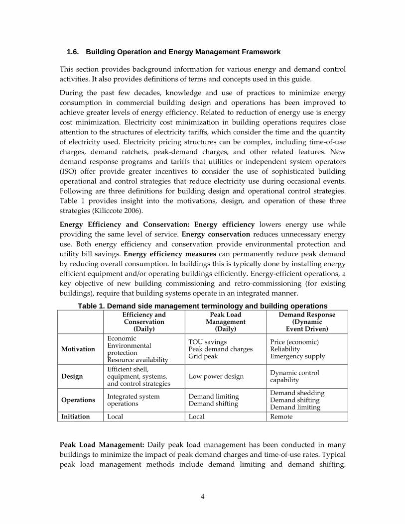
During  the  past  few  decades,  knowledge  and  use  of  practices  to  minimize  energy consumption  in  commercial  building  design  and  operations  has  been  improved  to achieve greater levels of energy efficiency. Related to reduction of energy use is energy cost minimization.  Electricity  cost minimization  in  building  operations  requires  close attention to the structures of electricity tariffs, which consider the time and the quantity of electricity used. Electricity pricing  structures can be complex,  including  time‐of‐use charges,  demand  ratchets,  peak‐demand  charges,  and  other  related  features.  New demand  response programs  and  tariffs  that utilities  or  independent  system  operators (ISO)  offer  provide  greater  incentives  to  consider  the  use  of  sophisticated  building operational and  control  strategies  that  reduce electricity use during occasional events. Following  are  three definitions  for building design  and operational  control  strategies. Table  1  provides  insight  into  the motivations,  design,  and  operation  of  these  three strategies (Kiliccote 2006). 

Energy  Efficiency  and  Conservation:  Energy  efficiency  lowers  energy  use  while providing  the  same  level of  service. Energy  conservation  reduces unnecessary energy use.  Both  energy  efficiency  and  conservation  provide  environmental  protection  and utility bill savings. Energy efficiency measures can permanently reduce peak demand by reducing overall consumption. In buildings this is typically done by installing energy efficient equipment and/or operating buildings efficiently. Energy‐efficient operations, a key  objective  of  new  building  commissioning  and  retro‐commissioning  (for  existing buildings), require that building systems operate in an integrated manner. 

Table 1. Demand side management terminology and building operations

 Efficiency and Conservation (Daily) 

Peak Load Management (Daily) 

Demand Response (Dynamic 

Event Driven) 

Motivation Economic Environmental protection Resource availability 

TOU savings Peak demand charges Grid peak 

Price (economic) Reliability Emergency supply 

Design Efficient shell, equipment, systems,  and control strategies 

Low power design  Dynamic control capability 

Operations  Integrated system operations 

Demand limiting Demand shifting 

Demand shedding Demand shifting Demand limiting 

Initiation  Local  Local  Remote 

 

Peak Load Management: Daily peak  load management has  been  conducted  in many buildings to minimize the impact of peak demand charges and time‐of‐use rates. Typical peak  load  management  methods  include  demand  limiting  and  demand  shifting. 

   

  5

Demand Limiting  refers  to shedding  loads when pre‐determined peak demand  limits are about to be exceeded. Demand limits can be placed on equipment (such as a chiller or  fan),  systems  (such  as  a  cooling  system),  or  a whole  building.  Loads  are  restored when the demand is sufficiently reduced. This is typically done to flatten the load shape when  the monthly peak demand  is pre‐determined. Demand  shifting  is  achieved  by changing  the  time  that  electricity  is used. Thermal  energy  storage  is  an  example of  a demand shifting strategy. Thermal storage can be achieved with active systems such as chilled water  or  ice  storage,  or with  passive  systems  such  as  pre‐cooling  of  building mass. In California, time dependent valuation (TDV)1 is also in use for building energy code  compliance  calculations  required  by  the  state  building  energy  code  (Title  24)  to take  into  account  the  time  that  electricity  is  used  during  the  year  (CEC  2005).  TDV acknowledges that some efficiency measures reduce summer peak electric demand more than others. 

Demand Response: Demand response is dynamic and event‐driven and can be defined as short‐term modifications  in customer end‐use electric  loads  in  response  to dynamic price  and  reliability  information.  Demand  response  programs may  include  dynamic pricing  and  tariffs,  price‐responsive  demand  bidding,  contractually  obligated  and voluntary curtailment, and direct load control or equipment cycling. As discussed above, Demand  limiting  and  shifting  can be utilized  for demand  response. DR  can  also be accomplished with demand shedding, which is a temporary reduction or curtailment of peak electric demand. Ideally a demand shedding strategy would maximize the demand reduction while minimizing any loss of building services.   

Figure  1  illustrates  concept  of  typical  electric  load  shapes  for  each  energy/demand control activity described above. 

                                                      

1 Time  dependent  valuation  (TDV)  is  an  energy  cost  analysis methodology  that  accounts  for variations in cost related to time of day, seasons, geography, and fuel type.  In California, under TDV  the value of electricity differs depending on  time‐of‐use  (hourly, daily,  seasonal) and  the value of natural gas differs depending on season. TDV is based on the cost for utilities to provide the energy at different times. 

   

  6

0

1

2

3

4

5

6

7

8

9

10

1:00

2:00

3:00

4:00

5:00

6:00

7:00

8:00

9:00

10:0

011

:00

12:0

013

:00

14:0

015

:00

16:0

017

:00

18:0

019

:00

20:0

021

:00

22:0

023

:00

0:00

Time of day

Bui

ldin

g de

man

d

Baseline

EnergyefficiencyDemandlimitingDemandsheddingDemandshifting

 * This chart is conceptual; the data are not from actual measurements. 

Figure 1. Examples of load shapes

Levels of Automation  for DR: Varying  levels of automation  for DR can be defined as follows.  Manual  Demand  Response  involves  a  labor‐intensive  approach  such  as manually  turning  off  or  changing  comfort  set  points  at  each  equipment  switch  or controller.  Semi‐Automated  Demand  Response  involves  a  pre‐programmed  load shedding strategy initiated by a person via centralized control system. Fully‐Automated Demand Response does not involve human intervention, but is initiated by an Energy Management Control System (EMCS) in a home, building, or facility through receipt of an external communications signal, receipt of which initiates pre‐programmed shedding strategies. 

Recent  evaluations  have  shown  that  customers  have  limited  knowledge  of  how  to operate their facilities to reduce their electricity costs under critical peak pricing or CPP (Quantum  and  Summit  Blue  2004). While  lack  of  knowledge  of  how  to  develop  and implement DR control strategies  is a barrier  to participation  in DR programs  like CPP, another barrier is the lack of automation in DR systems. Most DR activities are manual and require people to first receive emails, phone calls, and pager signals, and secondly for people to act on these signals to execute DR strategies (Piette 2006).

1.7. Terms and Concepts for DR Strategies

The  terms defined below describe key concepts of demand response control strategies. These terms are used throughout this report. 

Reduction in service: Demand response strategies achieve reductions in electric demand by  temporarily reducing  the  level of service  in  the  facility. HVAC and  lighting are  the systems most  commonly adjusted  to achieve demand  response  savings  in  commercial buildings. The goal of demand response strategies is to meet the demand savings targets while  minimizing  any  negative  impacts  on  the  occupants  of  the  buildings  or  the processes that they perform. 

   

  7

Occupant  satisfaction: Occupant  satisfaction  should  be maintained  by  adjusting DR strategies  to minimize  the reduction  in service, so  that  the occupants do not notice  the change in service (detectability), or at least so that the occupants can accept the changes (acceptability).  Many  studies  have  addressed  the  effect  of  temperature  changes  or lighting  changes  on  occupant  detectability,  acceptability,  and  task  performance.  Newsham  et  al.  conducted  an  extensive  literature  search  on  these  studies  (Newsham 2006). 

One common question regarding DR strategies  is: If you can use a strategy for a short period, why not use it all the time? Even if the occupants do not notice the reduction in service, the occupants’ productivity may be higher when the space conditions are closer to  the  occupants’ desirable  conditions. Differences  between  the  impacts  of  short‐term and  long‐term  space  condition  changes  are  yet  unknown.  Daily  demand  savings associated with reduction in service should be considered carefully. See Links to retro‐commissioning below for discussion of related topics. 

Shared burden: DR strategies  that share  the burden evenly  throughout  the  facility are least  likely  to  have  negative  effects  on  building  occupants.  For  example,  if  it  were possible to reduce lighting levels throughout an entire facility by 25% during a DR event, impacts  to occupants might be minimal. However,  turning off all of  the  lights  in one quadrant of an occupied  space would not be acceptable.  In HVAC  systems,  strategies that reduce load evenly throughout all zones of a facility are superior to those that allow certain areas (such as those with high solar gains) to substantially deviate from normal temperature  ranges. By  combining demand  savings  from  shed  in  each  component  of HVAC  and  lighting  systems  (and  other  loads,  if  available),  the  impact  on  each component is minimized and the demand savings potential is increased. 

Closed‐loop  control: Comfort  is maintained  in modern  buildings  through  the  use  of closed  loop  controls.  Sensors  are  used  to  measure  important  parameters  such  as temperature, and actuators adjust dampers or valves to maintain the desired setpoints. The effect of the valve or actuator on the controlled zone or system is measured by the sensor,  hence  closing  the  (control)  loop.  Control  sub‐systems  for  which  there  is  no feedback from sensors are known as open loop controls. 

To maintain predictable and managed reductions of service during DR events, strategies should maintain the use of closed loop control wherever possible. However, closed loop control  may  become  an  obstacle  to  achieve  demand  savings  when  the  final  target parameter  cannot  be  changed  through  centralized  control.  (For  example,  pneumatic control  systems  cannot  change  zone  setpoints  from  centralized  control, while  typical direct digital control systems can.) For instance, if supply air temperature is raised in a closed loop control system to reduce chiller demand, the fan speeds up to deliver more air  to  satisfy  the  zone  setpoints  and  fails  to  shed  HVAC  demand,  unless  the  zone setpoints are increased. 

Granularity  of  control:  For  the  purposes  of DR  control  in  buildings,  the  concept  of granularity refers to the amount of floor area covered by each controlled parameter (e.g. 

   

  8

temperature). If the space has many zones that can be separately controlled, the control strategy is considered highly granular. In HVAC systems, the ability to easily adjust the temperature setpoint of each occupied space  is a highly granular way  to distribute  the DR  shed  burden  throughout  the  facility.  Less  granular  strategies  such  as  making adjustments  to chillers and other central HVAC equipment can provide effective shed savings, but can cause temperature in some zones to drift out of control. Granularity of control  can  also  allow  building  operators  to  create  DR  shed  behaviors  that  are customized  for  their  facility. An example would be  to  slightly  increase all office zone temperature setpoints, but leave computer room setpoints unchanged.     

Resolution of control: Higher resolution of control increases the flexibility to adjust the level of DR control within a desirable range. Higher resolution of control also enhances the capability of ramping up  the change of DR control parameters. HVAC parameters can often be controlled with high resolution; in many systems temperature setpoints can be adjusted by as  little as 0.1°F. Although  some modern  fluorescent dimming ballasts can  adjust  individual  lamps  light  output  in  1%  increments,  most  commercial  lamp ballasts are only capable of turning lamps on or off. 

Rebound: At  the  end  of  each DR  event,  the  affected  systems must  return  to  normal operation. When  lighting  strategies  are used  for DR, normal operation  is  regained by simply re‐enabling all  lighting systems to their normal operation. Lights come back on as  commanded  by  time  clocks,  occupancy  sensors,  or manual  switches.  There  is  no reason for lighting power to jump to levels that are higher than normal for that period.   

However,  without  special  forethought,  HVAC  systems  tend  to  use  extra  energy following DR events to bring systems back to normal conditions. Extra energy is used to remove heat that is typically gained during the reduced service  levels of the DR event. This post DR event spike is known as rebound.  To minimize the chance of high demand charges and to reduce negative effects to the electric grid, rebound should be minimized through use of a graceful return to normal strategy. The simplest case is where the DR event ends or can be postponed until the building is unoccupied. If this is not possible, strategies  that  allow HVAC  equipment  to  slowly  ramp  up  or  otherwise  limit  power usage during the post‐DR period should be used. 

Links  to  retro‐commissioning: Assuming  the HVAC and  lighting systems are already operated to achieve optimal occupant satisfaction and minimize energy consumption in their  normal  operation,  the  implementation  of DR may  cause  a  reduction  in  service. However, there are many cases in reality where the systems are not operated optimally. In these cases, it may be possible to reduce electric demand without reduction in service. If a facility finds such a strategy, it should be considered a permanent energy efficiency opportunity rather than a temporary DR strategy, and should be performed on non‐DR days as well. 

Planning  a  DR  strategy  can  be  a  good  opportunity  to  examine  the  sequence  and parameters  of  building  control.  While  facility  managers  may  be  concerned  about deviations  from  current  operation  only  for  energy  efficiency,  they  may  be  more 

   

  9

motivated  if  the goal  is both  energy  efficiency  and DR because  the  occupants  can be more permissive under a DR situation in many cases. Once confirmed that the strategy does not negatively  impact the  level of service, the strategy can be operated on a daily basis. 

The LBNL Auto‐DR studies  found several cases where DR strategies merely  impacted the level of service and  incorporated the strategies in their daily operation (Piette et al. 2005a, 2005b, 2006). In one example, a duct static pressure reset strategy was used for a building with pneumatic zone  controls. Through  this  effort  to develop  short‐term DR strategies, the duct static pressure was reset to operate lower during all operating hours. In  another  case,  reduction  in  service  actually  improved  occupant  comfort  or productivity in some zones that were over‐cooled during normal operation. These cases can  be  viewed  as  classic  retro‐commissioning  opportunities,  identified  through  the process of developing DR  strategies.  In other  instances, when  examining  electric  load shapes,  the  team  found  equipment,  such  as  fans  or  process  equipment,  running unnecessarily at night. 

In addition, if systems in a facility are operating poorly due to design or commissioning issues,  it may  be more difficult  to  implement  effective DR  strategies.  For  example,  if zones  are  over‐cooled  due  to  excessive  minimum  airflows  or  low  supply  air temperatures,  raising  zone  temperature  setpoints  during  a  DR  event  will  not  save energy.   

DR strategy commissioning: The process of commissioning should be applied  to each phase  of  DR  control  strategy  application  including  planning,  installation,  and implementation to make sure that the goal of DR control ‐‐ to maximize demand savings and minimize impact to occupants ‐‐ is achieved. The commissioning procedure and key issues are described in Section 4.1. 

Design of DR  control  strategies would  ideally  take place during  the new  construction commissioning  phase  and  be  incorporated  into  the  commissioning  process.  A demonstration of  this  concept  is being planned at  the New York Times Headquarters building (Kiliccote et al. 2006).

   

 10

2. Demand Response Strategy Overview

This  section  provides  an  overview  of  demand  response  control  strategies.  These strategies  are  categorized  into  four  areas: HVAC,  lighting, miscellaneous  equipment, and non‐component‐specific measures. The details of each strategy are described in the following section. 

2.1. HVAC Systems

HVAC  systems  can be  an  excellent  resource  for DR  shed  savings  for  several  reasons. First, HVAC systems create a substantial electric demand in commercial buildings, often more  than one  third of  the  total demand. Second,  the  thermal  flywheel  effect of  indoor environments  allows HVAC  systems  to  be  temporarily  unloaded without  immediate impact to the building occupants. Third, it is common for HVAC systems to be at least partially automated with EMCS. 

However, there are significant technical challenges to using commercial HVAC systems to provide DR savings. These systems are designed to provide ventilation and thermal comfort  to  the  occupied  spaces.  Operational  modes  that  provide  reduced  levels  of service  or  comfort  are  rarely  included  in  the  original  design  of  these  facilities.  To provide  reliable,  repeatable DR  sheds  it  is  best  to pre‐plan  and  automate  operational modes  that  will  provide  DR  savings.  The  use  of  automation  reduces  labor  costs associated with the implementation of DR operational modes.   

HVAC‐based DR strategies recommended for a given facility vary based on the type and condition of the building, mechanical equipment, and EMCS. Based on these factors, the best DR  strategies are  those  that achieve  the aforementioned goals of meeting electric demand  savings  targets while minimizing  negative  impacts  on  the  occupants  of  the buildings or the processes that they perform. The following DR strategies are prioritized to achieve these goals: 

• Global Temperature Adjustment of Zones 

• Systemic Adjustments to the Air Distribution and/or Cooling Systems 

It  is  often  difficult  to  estimate  the  demand  savings  that will  be  achieved  by HVAC strategies, because HVAC cooling load is dynamic and sensitive to weather conditions, occupancy,  and  other  factors. However,  previous  research  has  found  that  the HVAC demand  and  its  demand  savings  tend  to  have  positive  correlation  with  outside  air temperature (OAT). 

In  all  field  tests  that  used HVAC‐based DR  strategies,  upon  initiation  of DR  events, temperatures  in  occupied  zones  drifted  from  normal  levels  at  rates well within  the acceptable rate of change specification allowed in ASHRAE Standard 55‐2004 (ASHRAE 2004). DR strategies used  to return HVAC systems  to normal operation should also be designed  to  limit  the  rate  of  temperature  change  so  as  to  not  exceed  the  ASHRAE standard. DR  strategies  that  slowly  return  the  system  to  normal  condition  have  the additional benefit of limiting rebound. 

   

 11

HVAC  strategies  can  be  categorized  by  the  system  targeted  for  control modification.  These include zone control, air distribution, and central plant, in order of recommended priority.  Where  practical,  DR  strategies  that  use  temporary  modifications  to  zone temperature setpoints are recommended. This recommendation is based on maximizing DR shed savings effectiveness while minimizing the potential for occupant discomfort.   

Figure 2 shows the basic concept of the HVAC DR strategy decision tree.  

START

Zonecontrol

DDC zonecontrol?

Y NDDC zonecontrol?

Y N

Central plantcontrol

Airdistribution

control

Air distributionSystem DDC?

Y NAir distributionSystem DDC?

Y N Central plantDDC?

Y NCentral plantDDC?

Y N

Do not try DRat this time

 Figure 2. HVAC DR strategy decision tree

Building HVAC types 

Building  HVAC  types  are  characterized  using  the  following  four  primary  system attributes and  the  secondary attributes  listed  in Table 2.The primary attributes are  (1) constant  air  volume  (CAV)  or  variable  air  volume  (VAV),  and  (2)  central  plant with chilled  water  system  or  packaged  units.  Applicable  DR  strategies  depend  on  these system  types.  Applicability  based  on  these  attributes  is  described  in  each  strategy section. Many of the  less‐common HVAC systems,  including water source heat pumps and gas cooling systems, are not included in this study. 

Table 2. Building HVAC types Type  Primary system attribute  Secondary system attribute 

Type A  CAV system with central plant (CAV‐Central) 

Single zone / multi‐zone Single duct / dual duct With reheat / without reheat Type of chiller 

Type B  VAV system with central plant (VAV‐Central) 

Single duct / dual duct With reheat / without reheat Type of chiller 

Type C  CAV system with package units (CAV‐Package) 

Single zone / multi‐zone Single duct / dual duct With reheat / without reheat 

Type D  VAV system with package units (VAV‐Package) 

Single duct / dual duct With reheat / without reheat 

CAV: Constant air volume   VAV: Variable air volume 

   

 12

Table 3 provides  short definitions of DR  strategies and  their applicability by building HVAC  type. One can  find a building HVAC  type  that  is  the closest  to one’s building, and  look for those strategies that are appropriate. Even  if the HVAC type matches, the strategies listed here may or may not be feasible, depending on the control attributes of your building.  

Table 3. HVAC demand response strategies Category  DR Strategy  Definition  A  B  C  D

Global temperature adjustment 

Increase zone temperature setpoints for an entire facility 

X  X  X  X 

Zone control  Passive thermal 

mass storage 

Decrease zone temperature setpoints prior to DR operation to store cooling energy in the building mass, and increase zone setpoints to unload fan and cooling system during DR. 

X  X  X  X 

Duct static pressure decrease 

Decrease duct static pressure setpoints to reduce fan power. 

  X    X 

Fan variable frequency drive limit 

Limit or decrease fan variable frequency drive speeds or inlet guide vane positions to reduce fan power. 

  X    X 

Supply air temperature increase 

Increase SAT setpoints to reduce cooling load. 

X  X  X  X 

Fan quantity reduction 

Shut off some of multiple fans or package units to reduce fan and cooling loads. 

X  X  X  X 

Air distribution 

Cooling valve limit  Limit or reduce cooling valve positions to reduce cooling loads. 

X  X     

Chilled water temperature increase 

Increase chilled water temperature to improve chiller efficiency and reduce cooling load. 

X  X     

Chiller demand limit  Limit or reduce chiller demand or capacity.  X  X     Central plant 

Chiller quantity Reduction  Shut off some of multiple chiller units.  X  X  *  * 

Slow recovery  Slowly restore HVAC control parameters modified by DR strategies. 

**  **  ** **

Sequential equipment recovery 

Restore HVAC control to equipment sequentially within a certain time interval. 

**  **  ** **Rebound avoidance 

Extended DR control Period 

Extend DR control period until after the occupancy period. 

**  **  ** **

* The strategy can be applied to package systems by reducing shutting off some of the compressors. ** Applicability of rebound avoidance strategies is determined by the DR strategies selected. 

Zone control strategies – Global Temperature Adjustment 

This  strategy  requires  zone  level  direct  digital  control  (DDC)  that  can  be  easily programmed to respond globally to demand response commands. Some control system manufacturers provide products  that enable  the zone setpoints of all  thermostats  to be changed  globally  by  one  parameter.  This  software  feature  is  known  as  global temperature adjustment (GTA). For control systems that do not offer GTA as a standard feature, it can usually be programmed during the installation or retrofit process, at a cost 

   

 13

somewhat higher  than  if  it were a standard  feature. This strategy has proven  to be an effective and minimally‐disruptive technique for achieving HVAC demand response. 

Air distribution strategies 

In systems for which global temperature adjustment of zones  is not an option (such as those  that  are  not  DDC),  strategies  that  make  temporary  adjustments  to  the  air distribution or mechanical cooling systems can be employed to enable demand response. If the HVAC (fans, chillers, or both) is a constant volume system (without VAV), direct control of the equipment may be considered.  

If  the  HVAC  system  is  VAV,  a  combination  of multiple  parameter  controls  can  be considered. Within a  closed  loop  system,  fans and  chillers always  try  to maintain  the required  set  points  by  changing  HVAC  parameters.  For  example,  a  supply  air temperature (SAT) increase might reduce chilled water flow to save cooling energy, but fan power might rise to increase airflow to maintain cooling zone set points at the VAV boxes  (which  try  to  compensate  for warmer  supply  air  by  supplying more  air).  To achieve  a  demand  reduction,  the  fan  and  chiller  control  strategies  may  require simultaneous modifications.  One may want  to  limit  or  fix  the  chilled water  supply temperature,  and  simultaneously  limit  or  fix  the  variable  frequency  drive  (VFD) percentage to reduce fan power. 

While  effective  in  achieving  load  reductions,  the  use  of  systemic  adjustments  to  air distribution  systems  and/or  mechanical  cooling  systems  for  DR  purposes  has  some fundamental  drawbacks.    In  these  strategies,  the  DR  burden  is  not  shared  evenly between  all  the  zones.  Centralized  systemic  HVAC  DR  shed  strategies  can  allow substantial deviations  in  temperature, airflow, and ventilation rates  in some areas of a facility. Centralized systemic changes  to  the air distribution system and/or mechanical cooling  systems  allow  zones with  low  demand  or  those  that  are  closer  to  the main supply  fan  to  continue  to  operate  normally  and  hence  these  zones do  not  contribute toward load reduction in the facility. Zones with high demand, such as the sunny side of the building or zones at the ends of long duct runs, can become starved for air. After a VAV  box  is  fully  opened,  its  zone  setpoint  is  no  longer  under  control.  Increased monitoring of occupied areas should be conducted when using these strategies.   

Cooling strategies 

Most  modern  centrifugal,  screw,  and  reciprocating  chillers  have  the  capability  of reducing  their power demands. This  can be done by  raising  the  chilled water  supply temperature  setpoint  or  by  limiting  the  speed,  capacity, number  of  stages,  or  current draw of the chiller. The number of chillers running can also be reduced in some plants.  As  mentioned  above,  reducing  the  central  plant  load  can  typically  achieve  larger demand  savings  than  can  be  achieved  by  reducing  the  air  distribution  load.  These strategies may cause some air distribution  load  increases, which are usually more than compensated for by central plant load reductions. 

   

 14

Rebound avoidance strategies 

As mentioned  in  section  1.7, HVAC  systems  tend  to  experience  rebound, using  extra energy  following DR  events  in  order  to  bring  systems  back  to normal  conditions. To minimize  the  chance  of  high  demand  charges  and  to  reduce  negative  effects  on  the electric  grid,  rebound  should  be minimized  through  use  of  a  gradual  return  to  the normal strategy. The simplest case is where the DR event ends or can be postponed until the building is unoccupied. If this is not possible, strategies that allow HVAC equipment to  slowly  ramp up or otherwise  limit power usage during  the  return  to normal  state should be used.

2.2. Lighting Systems

On a hot summer day when daylight  is abundant, daylit and/or over‐lit buildings are the  best  candidates  for  demand  reduction  using  the  lighting  system.  Since  lighting produces heat, reducing lighting levels will also reduce the cooling load within the space and  allow  the HVAC  strategies  to work  for  extended  periods  of  time.  Research  has shown that each kWh of lighting savings can also provide additional cooling savings by reducing  the  cooling  load.  This  savings  varies  in  quantity  by  building  type  and characteristics, climate zone, and season of the year. An LBNL study estimated that, on a national annual average, 1 kWh  lighting savings  induces 0.48 kWh cooling savings  for existing commercial buildings (Sezgen and Koomey 1998). 

Lighting demand shed strategies  tend  to be simple and depend widely on wiring and controls infrastructures. However, since lighting is typically associated with health and safety and the shed strategies tend to be visible, they have to be carried out selectively and carefully considering the tasks perfomed in the space and ramifications of reduced lighting for the occupants. Typically, the resolution of lighting controls tends to be lower than that of HVAC controls. Also, lighting systems are often not automated with EMCS. These  issues can be major obstacles  for automation of  lighting DR strategies, although lighting strategies are popularly used in manual DR. 

Estimating  the  demand  savings  potential  of  lighting  strategies  depend  on  how  the demand savings are achieved. Demand response control capability of lighting systems is generally determined by the characteristics of lighting circuit and control system. There are  two ways  to  implement demand  response  control with  lighting,  absolute  reduction and  relative  reduction. Absolute  reduction  is  achieved by programming preset  lighting level  for  times when demand  response  is  required. This may  be  configured  in many different ways based on the lighting control strategies, i.e. half the fixtures on, one third of the lamps in each fixture on, or all lamps at 70% of full light output.   

The problem with an absolute reduction approach is that it does not yield any savings or may even increase lighting electricity consumption if the lighting levels are the same as or  lower  than  the  preset  levels  at  the  time  demand  response  is  initiated.  Therefore, although this approach  is easy to  implement with current  lighting control systems, the demand savings estimate varies depending on the building use and occupancy. 

   

 15

Relative reduction means reducing loads with respect to the level of lighting at the time of demand  response.  Instead of  reducing  to a preset  level, a certain percent  reduction over  the  current  value  is  achieved during  a demand  response  event.  Implementation requires  that  the  light  output  from  the  lamp  or  power  output  from  the  ballast  is communicated  back  to  the  lighting  control  system,  so  central  closed  loop  control  is required. Systems with such sophisticated controls tend to be newer and more expensive. The  decision  to  implement  absolute  or  relative  lighting  reduction  depends  on  the building  lighting  infrastructure, the  lighting use  in the building, and the capabilities of the installed lighting control system. 

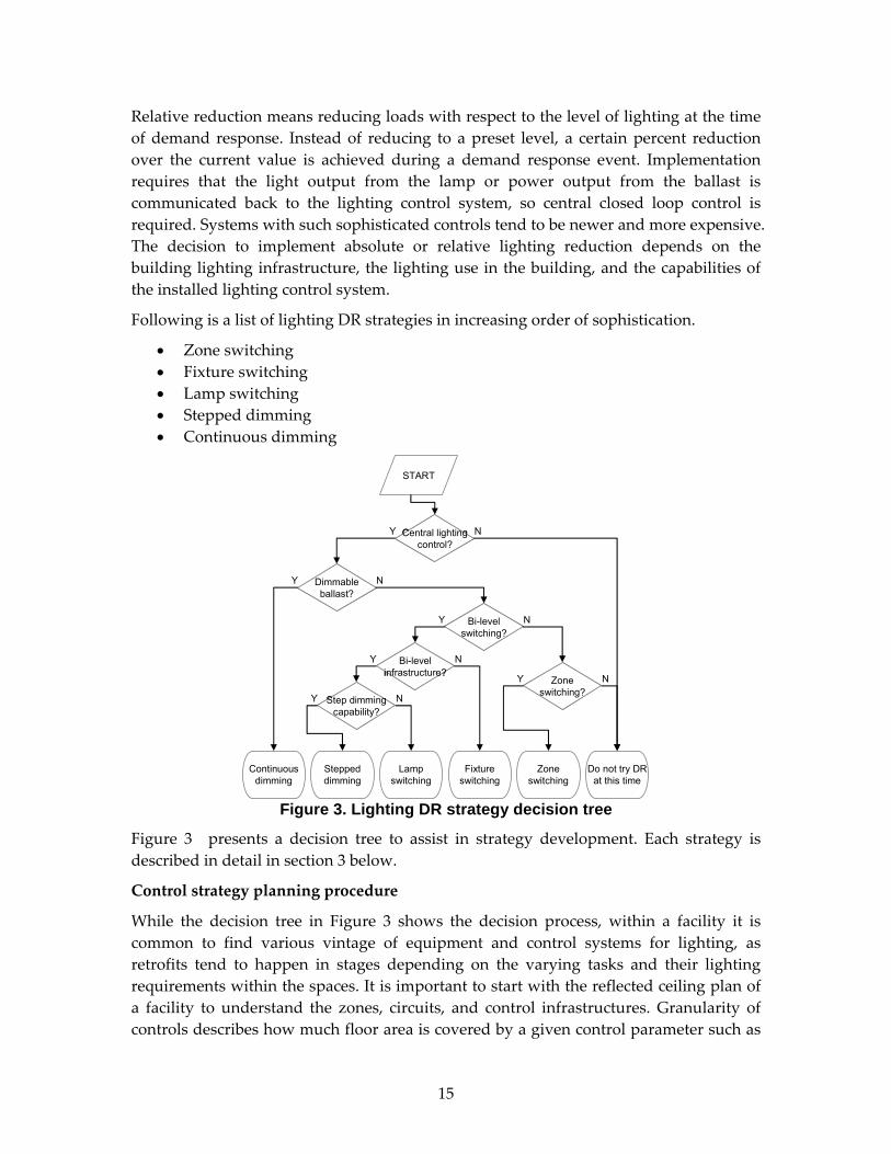
Following is a list of lighting DR strategies in increasing order of sophistication.  

• Zone switching • Fixture switching • Lamp switching • Stepped dimming • Continuous dimming 

START

Central lightingcontrol?

Y NCentral lightingcontrol?

Y N

Dimmableballast?

Y NDimmableballast?

Y N

Zoneswitching

Zoneswitching?

Y NZoneswitching?

Y N

Bi-levelswitching?

Y NBi-levelswitching?

Y N

Do not try DRat this time

Fixtureswitching

Continuousdimming

Lampswitching

Steppeddimming

Bi-levelinfrastructure?

Y NBi-levelinfrastructure?

Y N

Step dimmingcapability?

Y NStep dimmingcapability?

Y N

 Figure 3. Lighting DR strategy decision tree

Figure  3 presents  a decision  tree  to  assist  in  strategy development. Each  strategy  is described in detail in section 3 below. 

Control strategy planning procedure 

While  the decision  tree  in  Figure  3  shows  the decision  process, within  a  facility  it  is common  to  find  various  vintage  of  equipment  and  control  systems  for  lighting,  as retrofits  tend  to  happen  in  stages  depending  on  the  varying  tasks  and  their  lighting requirements within the spaces. It is important to start with the reflected ceiling plan of a  facility  to understand  the  zones,  circuits,  and  control  infrastructures. Granularity of controls describes how much floor area is covered by a given control parameter such as 

   

 16

a  photosensor.  Less  granular  strategies  affect more  occupants  and  tend  to  be more disruptive.  More  granular  strategies  require  well‐designed  and  well‐implemented infrastructures and allow occupants to better accept DR strategy implementation.   

2.3. Miscellaneous Equipment

DR  can  target  other  equipment  besides  HVAC  and  lighting.  If  the  equipment  is independent from any critical operation, the sequence of control does not require such careful  consideration.  One  issue  of  shedding  miscellaneous  equipment  is  that  this equipment  is often not  connected  to  the EMCS but  rather  is operated  stand‐alone.  In commercial buildings, the demand response potential of miscellaneous equipment shed is  usually  insignificant  compared  to HVAC  or  lighting  shed. On  the  other  hand,  in industrial sites, significant demand reduction can be achieved by temporally unloading process loads without jeopardizing the process or product quality 

2.4. Non-Component-Specific Control Strategies

The  demand  response  control  strategies  mentioned  above  can  be  controlled  in  a sophisticated manner with the use of an advanced EMCS. Combination of DR strategies are  programmed  in  the  EMCS  to  coordinate  appropriate  strategies  based  on  various conditional parameters such as outside air  temperature, whole building demand  level, or electricity price level. These strategies may require a high level of programming effort.

2.5. Strategies Used in Case Studies

Table 4 and Table 5 summarize the DR strategies used during 4 years in the LBNL Auto‐DR studies and  the other case studies. The  list contains 56 participants (35 commercial and  9  industrial  buildings). All  40  LBNL  project  sites  implemented  the  strategies  as fully‐automated DR, while the other case studies used either manual or semi‐automated DR. 

   

 17

Table 4. DR strategies used in LBNL Auto-DR studies (fully-automated)

Building use 2003

2004

2005

2006

Glo

bal t

emp.

adj

ustm

ent

Duc

t sta

tic p

res.

Incr

ease

SA

T In

crea

se

Fan

VFD

lim

it

CH

W te

mp.

Incr

ease

Fan

qty.

redu

ctio

n

Pre

-coo

ling

Coo

ling

valv

e lim

it

Boi

ler l

ocko

ut

Fan-

coil

unit

off

Ele

ctric

hum

idifi

er o

ff

Chi

ller d

eman

d lim

it

Slo

w re

cove

ry

Ext

ende

d sh

ed p

erio

d

Com

mon

are

a lig

ht d

im

Offi

ce a

rea

light

dim

Turn

off

light

Dim

mab

le b

alla

st

Bi-l

evel

sw

itchi

ng

Ant

i-sw

eat h

eate

r she

d

Foun

tain

pum

p of

f

Non

-crit

ical

pro

cess

she

d

Office ● ● XOffice ● XOffice ● X XOffice ● XOffice ● X X X X XOffice ● X X X X XOffice ● ● ● X XOffice ● ● ● X XOffice ● ● XOffice ● ● X XHi-tech office ● ● ● X X X X X X X XHi-tech office ○ XOffice, data center ● ● ● ● X X X X XOffice, data center ● X XOffice, lab ● X X X X X XOffice, lab ● ● X X X X X X XOffice, lab ● ● X XOffice, lab ● ● X XResearch facility ● X XCafeteria, auditorium ● ● XArchive storage ● XLibrary ● ● X X XHighschool ● ● X XJunior Highschool ○ X XDetention facility ● XRetail ● ● X X X XRetail ● X XRetail ● X XRetail ● X XFurniture retail ● ● XFurniture retail ○ XSupermarket ● X X XSupermarket ○ XSupermarket ○ XSupermarket ○ XMuseum ● ● X XDistribution center ● ○ ○ X XManufacture, office ○ X XBakery ● XMaterial process ● X

Participation HVAC Lighting Other

 * Some sites participated in 2003 or 2004 study stopped due to ineligibility to participate in CPP. * In the Participation column, ● indicates the year of participation, and ○ indicates that the site was in the process of developing the DR strategies indicated in columns to the right. 

   

 18

Table 5. DR strategies used in case studies (manual or semi-automated)

Building useRerefenced

studies Glo

bal t

emp.

adj

ustm

ent

Duc

t sta

tic p

res.

Incr

ease

SAT

Incr

ease

Fan

VFD

lim

it

CH

W te

mp.

Incr

ease

Fan

qty.

redu

ctio

n

Pre

-coo

ling

Fan-

coil

unit

off

Chi

ller d

eman

d lim

it

Chi

ller q

ty. r

educ

tion

Com

mon

are

a lig

ht d

im

Offi

ce a

rea

light

dim

Turn

off

light

Dim

mab

le b

alla

st

Bi-l

evel

sw

itchi

ng

Non

-crit

ical

pro

cess

she

d

Ele

vato

r cyc

ling

Shu

t off

cold

sto

rage

Ww

ater

pum

p pe

ak s

hift

Office Quantum X X XOffice Quantum X X X X X X XFood process Quantum X X XGlass process Quantum XChemical repackage Quantum X X XPacking & cold storage Quantum X X X XPacking & cold storage Quantum X XRetail NYSERDA X XCement process NYSERDA XOffice NYSERDA X X XIrrigation NYSERDA XLumber process SCE XOffice SCE X XOffice DOE Project X X X X X X X XLibrary ISO New England X X

HVAC Lighting Other

 Figure 4 illustrates the number of sites for each strategy used. The most popular strategy used was global  temperature adjustment, of which nearly half of  the  listed sites used. Duct static pressure increase and SAT increase were the second‐most popular strategies. 

0 5 10 15 20 25

Global temp. adjustment

Duct static pres. Increase

SAT Increase

Fan VFD limit

CHW temp. Increase

Fan qty. reduction

Pre-cooling

Cooling valve limit

Turn off light

Dimmable ballast

Bi-level switching

# of sites

Fully-Automated Manual or Semi-Automated 

Figure 4. Frequency of DR strategies

   

 19

3. Demand Response Strategy Detail

This section describes the details of the system operation methods of demand response strategies. Each strategy  is explained with system requirements, sequence of operation and specific  issues  to consider. The  information  is  first summarized  in  table  form and then explained below. 

3.1. HVAC Systems

This section describes the details of HVAC DR control strategies. Table 6 through Table 15 summarize the key information on the strategy, and the details are explained below the table.  Definitions of items in the table are listed below, 

• Definition – Brief definition of the DR control strategy. 

• HVAC type – Applicable HVAC types as defined in Table 2.  

• Target  loads  – HVAC  system  component  or  equipment whose  electric  load  is targeted to be reduced by the DR strategy. 

• Category  –  DR  approach:  demand  shed,  demand  shift,  or  demand  limit  as defined in Section 1.6. 

• System applicability – HVAC or control system characteristics required  to use the DR strategy. 

• Sequence  of  operation  – Detailed  sequence  of  operation used  to program  the EMCS to implement the DR control strategy. 

• EE potential – Potential of achieving savings  from energy efficiency as well as DR by applying the DR strategy during regular practice outside of DR events.  

• Rebound – Risk of  rebound peak and necessity of  rebound avoidance strategy from applying the DR strategy. 

• Cautions  –  Miscellaneous  issues  to  be  considered  when  the  DR  strategy  is applied to mitigate and avoid any risks. 

• Applied  sites  – Number  and  building  type  of  the LBNL Auto‐DR participant sites  that  applied  the  DR  strategy.  None  indicates  the  DR  strategy  was  not implemented  at  the  LBNL  Auto‐DR  sites,  but  was  used  in  some  other  case studies or at an  ex‐candidate  site  that  implemented  the  strategy but  could not automate it. 

   

 20

3.1.1. Global temperature adjustment Table 6. Conditions for global temperature adjustment (GTA)

Definition  Increase zone temperature setpoints for an entire facility. HVAC type  All Target loads  Air distribution, cooling Category  Demand shed 

System applicability 

1. DDC zone control 2a. Global temperature adjustment (GTA) capability at zone level, or 2b. Capability to program GTA at each VAV box. Option 1: Absolute setpoint adjustment Globally adjust (increase) all zone cooling setpoints to a common value (e.g. 76°F ), Tc°F Globally adjust (decrease) or leave unchanged all zone heating setpoints to a common value (e.g. 68°F), Th °F (Tc: DR mode cooling setpoint, Th: DR mode heating setpoint) Sequence of 

operation  Option 2: Relative setpoint adjustment Globally adjust (increase) all zone cooling setpoints by a common differential temperature from their prior setpoint (e.g. 2°F ), Tc°F Globally adjust (decrease) or leave unchanged all zone heating setpoints by a common differential temperature from their prior setpoint (e.g. 2°F ), T h°F  (Tc: DR mode cooling setpoint, Th: DR mode heating setpoint) 

EE potential  Some occupants may be more comfortable during DR events.  This would indicate making permanent changes to the setpoints.    

Rebound  Rebound avoidance strategy required. 

Cautions  Adjust zone temperature setpoints in multiple steps if a long shed duration is required.   

Applied sites 15 office buildings, 6 retail stores, 2 laboratory facilities, 2 schools, 1 manufacturing facility, 1 museum, 1 archive storage, 1 detention facility 

Global  Temperature  Adjustment  (GTA)  of  occupied  zones  is  a  strategy  that  allows commercial building operators  to  easily adjust  the  space  temperature  setpoints  for an entire facility by one command from one location. Typically, this is done from a screen on the human machine interface (HMI) to the EMCS. In field tests, GTA was shown to be the most  effective  and  least  objectionable  strategy  of  the HVAC DR  strategies  tested (Piette et al. 2005a, 2005b, and 2006). It is most effective because it reduces the load of all associated air handling and cooling equipment. It is least objectionable because it shares the burden of reduced service level evenly between all zones. GTA‐based DR strategies can  be  implemented  either  automatically  based  on  remote  signals  or  manually  by building operators.   

   

 21

GTA  is  typically  implemented  by  broadcasting  a  signal  from  the  central  EMCS HMI server to all the endpoint space temperature control devices distributed throughout the facility. Upon  receipt of a global  signal  from  the  central EMCS  server,  the  final  space temperature control devices interpret the signal and react accordingly. (For example, the global signal for DR Mode Stage‐1 means to increase space cooling setpoints 3°F and to decrease space heating setpoints 3°F). Final space  temperature control devices suitable for  GTA  include:  1)  space  temperature  controllers  that  adjust  VAV  terminal  box dampers  (e.g.  VAV  boxes),  2)  space  temperature  controllers  that  adjust  hot  water heating  coil  valves  or  chilled water  cooling  coils  (e.g.  fan  coil units, CAV multi‐zone heating,  and  cooling  coil  valves)  and  3)  space  temperature  controllers  that  adjust  the capacity of heat pumps or direct expansion (DX) units.   

To  avoid  an  unwanted  increase  in  heating  energy,  heating  setpoints  (if  any)  should remain the same or be reduced during GTA mode. Otherwise, raising cooling setpoints could also raise heating setpoints, and may cause heating operation to be started.  

GTA may  be  implemented  on  either  an  absolute  or  relative  basis. Absolute  setpoint adjustment of GTA allows  the operator  to  set  the  space  temperature  setpoints  for  the entire  facility  to  absolute  values  (e.g.  heating  setpoints  at  all  final  space  temperature control  devices  =  68°F  and  cooling  setpoints  at  all  final  space  temperature  control devices = 76°F). Relative setpoint adjustment of GTA allows  the operator  to adjust  the space temperature setpoints for the entire facility to new values that are offset from the current values by a relative amount (e.g. heating setpoints at all final space temperature control devices decrease 2°F from current values and cooling setpoints increase 2°F from current values). 

While  being  implemented,  the  rate  of  increase  in  temperature  in  the  spaces  should comply with the temperature drift rate allowed under ASHRAE Standard 55 as outlined in the Figure 5: 

 

Several manufacturers offer GTA as a standard feature  in their EMCS products. EMCS without  the  GTA  feature  can  adjust  space  temperature  setpoints  in  each  zone individually, but not globally. Adjusting each zone  individually  is too time‐consuming and  error‐prone  for DR purposes.  In  field  tests,  sites  that used EMCS products  from 

Time Period2 ºF -15 minutes3 ºF - 30 minutes4 ºF - 1 hour5 ºF - 2 hours6 ºF - 4 hours

ASHRAE 55-2004, Paragraph 5.2.5.2Change in Temperature

Time Period2 ºF -15 minutes3 ºF - 30 minutes4 ºF - 1 hour5 ºF - 2 hours6 ºF - 4 hours

ASHRAE 55-2004, Paragraph 5.2.5.2Change in Temperature

Figure 5. Temperature drift rate allowed under ASHRAE Standard 55 

   

 22

these vendors provided some of the largest sheds and required the least amount of set‐up labor.   

For  sites  that  have  EMCS  controlled  space  temperature  zones,  but  lack GTA,  it  can typically  be  added  in  the  field.  To  add  GTA  to  an  existing  site,  each  EMCS  zone controller must be programmed to “listen” for a global GTA command from the central EMCS  system.  In  addition,  the  central  system  must  be  programmed  to  send  GTA commands to all relevant zone controllers on the EMCS digital network. Typically GTA commands are sent in a global broadcast to all controllers simultaneously. 

Manufacturers offer different  types of VAV zone  setpoint  configuration methods. The following two examples are common VAV zone setpoint configurations. 

1. Define zone cooling setpoints and zone heating setpoints separately. 

2. Define the midpoint between zone cooling setpoints and zone heating setpoints and the width of the deadband.2 Increasing the deadband makes cooling setpoints higher  and  heating  setpoints  lower. Raising  the midpoint makes  both  cooling and heating  setpoints higher. Figure 6  shows  the  change  in  the deadband and required  airflow  change  in  a  VAV  system. 3   Increasing  the  cooling  setpoints reduces the required airflow. 

Heatingsetpoint

Coolingsetpoint

MinCFM

Airf

low

CFM

Deg-FThNew

setpoint

TcNew

setpoint

Originaldeadband

New deadband

∆Th∆Th ∆Tc∆Tc

Setpoint-airflow relationshipwith original deadband

Setpoint-airflow relationshipwith new deadband

 Figure 6. Zone setpoints deadband

                                                      2 Deadband  in  the  context of zone  temperature  control has  two definitions; 1)  the  temperature range  between  actuation  and  de‐actuation  of  the  cooling  or  heating  system,  and  2)  the temperature  range where no  cooling or heating  (beyond  that  required  to provide  fresh  air)  is provided. Although  the  first definition has been historically used,  the second definition  is also commonly used. This report uses the second definition. 

3  Figure  5  shows  proportional  control  for  illustrative  purposes.    Most  zone  controllers  use proportional and integral control algorithms.   

   

 23

If GTA of zones is available, it is the recommended HVAC DR strategy for commercial buildings. In field tests, sites that used HVAC DR strategies other than GTA usually did so because that feature was not available at the site. Reasons that GTA was not available include: 1) Space  temperature was not controlled by  the EMCS  (e.g. use of pneumatic controls in occupant zones), and 2) Space temperature was controlled by the EMCS, but the space temperature controllers did not include the GTA feature.   

While the GTA strategy reduces the service level of the occupied spaces, it does so using a  closed‐loop  control  strategy  in  a  highly  granular  fashion.  This  causes  the DR  shed burden  to be evenly shared between all building occupants and keeps all zones under control. Since none of  the zones are  starved  for airflow,  there  is no  risk of ventilation rates dropping below specified design levels. 

Sometimes if the HVAC systems are oversized and the chillers are not controlled by the percentage  of  zones  asking  for  cooling,  the  GTA  strategy  has  to  be  combined with supply air  temperature  reset. One  typical example  is a building with multiple  rooftop units, where the compressors are controlled not by how many zones are directly asking for  cooling,  but  by  meeting  the  supply  air  temperature  setpoints.  If  the  units  are oversized or the minimum supply air flow rate is too high, GTA may not work and the zone  temperatures will not  follow  the new  setpoints because of  the  excessive  cooling provided by  the minimum air  flow.  In  that case,  the SAT setpoint has  to be  increased about 3~5oF in the GTA period to reduce the minimum cooling delivered by the HVAC system.  

The GTA  strategy works well with most built‐up HVAC  systems, where  typically  the chillers shut off if the percentage of zones that ask for cooling is less than a predefined threshold. In GTA, if no zones ask for cooling once the new setpoint is above the current zone  temperatures,  the chillers normally shut off automatically. Sometimes,  instead of being  completely  shut  off,  the  chillers will  only  be  reduced  to  a  partial  capacity,  to maintain cooling for some “hot spots” that are poorly balanced or otherwise overloaded.   

Thermal zones that are poorly designed or poorly balanced can also pose challenges due to overcooling.  If minimum  fresh  air  requirements  are overcooling many  zones,  shed savings from a GTA DR strategy alone may not be effective. This problem can be solved by  increasing  the  supply  air  temperature  in  addition  to  raising  the  zone  temperature setpoints.   

Demand savings components of GTA 

Demand  savings by  the GTA  strategy  consists of  two parts,  steady‐state  savings and transient savings.  When zone setpoints are raised, cooling is turned off or reduced to its minimal operation until zone temperatures reach the new setpoints (transient savings).  After  zone  temperatures  are  stabilized  at  the  new  setpoints,  the  cooling  load  is  still lower than the baseline cooling load due to a smaller difference between zone setpoints and OAT (steady‐state savings). 

   

 24

Transient  savings  can  be  achieved  by  the  thermal  mass  storage  effect  of  building structure mass, including floor slab and interior‐and‐exterior walls, furniture, and other materials. When  zone  setpoints  are  increased  by  the GTA  strategy,  the  thermal mass components have  stored  cooling energy. The  thermal mass  cools down  the  indoor air and displaces  the  cooling  load until  it  runs out of  stored  cooling  energy. Duration of transient  savings  can widely  vary depending  on  factors  including  building  structure, outside air flow rate, internal heat gain, and solar heat gain through windows.  

Figure 7  illustrates a conceptual diagram of demand savings  (not actual  field data) by the GTA strategy with zone setpoint (ZT set point) increase from 72°F to 76°F.   The zone temperture  (ZT  read)  is  also  shown.   A  case  study  of  this  strategy  is  introduced  in Appendix A, section A.1. 

 

 

0

100

200

300

400

500

11:0

0

11:3

0

12:0

0

12:3

0

13:0

0

13:3

0

14:0

0

14:3

0

15:0

0

15:3

0

16:0

0

16:3

0

17:0

0

17:3

0

18:0

0

18:3

0

19:0

0

Time

Who

le B

uild

ing

Pow

er [k

W]

70

75

80

85

90

95

Tem

pera

ture

[°F]

Baseline DR demand ZT SP ZT read

Transient Savings

Steady-State Savings

Figure 7. Conceptual diagram of demand savings for typical HVAC-based demand

response strategy

 

 

 

 

 

   

 25

3.1.2. Passive thermal mass storage Table 7. Conditions for passive thermal mass storage

Definition Decrease zone temperature setpoints during off‐peak hours prior to a curtailment to store cooling energy in the building mass, and then increase zone setpoints to unload fan and cooling system during a curtailment. 

HVAC type  All 

Target loads  Air distribution, cooling 

Category  Demand shift or demand shed 

System applicability 

1. DDC zone control 2a. Global temperature adjustment (GTA) capability at zone level, or 2b. Capability to program GTA at each VAV box. 3. Medium to high building mass. 

Sequence of operation 

Decrease zone temperature setpoints by ΔTc1 °F prior to a curtailment. Increase zone temperature setpoints by ΔTc2°F during a curtailment. 

EE potential Occasionally produces total energy usage savings in mild climates, especially when nighttime free ventilation cooling is used.  However, total energy usage may increase depending on climate, building type, and pre‐cooling schedule. 

Rebound  Rebound avoidance strategy required. 

Cautions 

This strategy is applicable to day‐ahead DR programs, where the event notification is sent on the day before.  If the event notification is on the same day, there is not sufficient time to store enough cooling energy.  The passive thermal mass storage control is very complicated and has to be done properly.  Testing, adjusting, and balancing control schedules are recommended in the preparation phase. Avoid over‐cooling during the pre‐cooling period to prevent cold complaints from occupants. 

Applied sites  1 office building, 1 museum 

Pre‐cooling  the  thermal mass of  the building can be used  to reduce  the peak  load. For example, in summer, the building mass can be cooled during non‐peak hours to reduce the cooling load in the peak hours. As a result, the cooling load is shifted in time and the peak  demand  is  reduced.  The  building mass  can  be  cooled most  effectively  during unoccupied hours because it is possible to relax the comfort constraints. 

Thermal mass control strategies differ  in  the way  they store and release heat  from  the mass. The building mass may be cooled by natural or mechanical ventilation, with or without mechanical cooling. Pre‐cooling can be performed either during the unoccupied hours or during the occupied non‐peak hours, usually in the morning. In climates with a large  diurnal  temperature  swing,  it  may  be  possible  to  pre‐cool  the  building  mass without mechanical cooling. 

If there is sufficient pre‐cooling and the daytime cooling load is relatively low, it may be possible  for  the  indoor air  temperature  to remain within  the comfort range during  the peak hours without any mechanical cooling. Cooling energy stored  in  the mass can be discharged during the peak hours by either zonal temperature reset or demand limiting the cooling plant and distribution system (Xu 2004). A detailed simulation study of the passive thermal mass storage strategy is summarized in Appendix A, section A.2 (Braun et al. 2001).  

   

 26

3.1.3. Duct static pressure decrease Table 8. Conditions for duct static pressure decrease

Definition  Decrease duct static pressure (DSP) setpoints to reduce fan power. HVAC type  B (VAV‐Central), D (VAV‐Package) Target loads  Air distribution, cooling (occasionally) Category  Demand shed System applicability 

1. All zone control systems including pneumatic and DDC 2. DDC for air handling unit 

Sequence of operation  Lower DSP setpoints by X%. 

EE potential  Tuning DSP setpoints can save fan power consistently without a reduction in service. 

Rebound  Rebound avoidance strategy required. 

Cautions  Less airflow for some zones that may cause ventilation rates to drop below specified design levels. 

Applied sites  5 office buildings, 1 library 

For VAV systems, duct static pressure  (DSP)  is  typically measured  in  the supply duct. The EMCS modulates the speed of the fan or the position of inlet guide vanes (IGV) to maintain defined DSP  setpoints  at  the measured  locations. The normal DSP  setpoints should  be  high  enough  to  provide  enough  pressure  for  each  terminal  VAV  box  to function properly. Typically DSP is measured at a single location about two‐thirds of the way  down  the  duct  system.  The DSP  setpoints  are  set  to  fixed  values  that  are  high enough  to meet  the  needs  of  the  box  of  greatest  demand  during  design  conditions. During less demanding conditions energy may be wasted due to losses associated with the DSP setpoints being higher than necessary to meet demands of VAV boxes.   

Fan energy and cooling energy can be reduced during DR events by reducing the DSP setpoints. This strategy is effective for three reasons:  

1. Unless  the building has been recently commissioned,  the normal DSP setpoints are  often  higher  than  necessary.    By  reducing  the  DSP  setpoints,  some  shed savings is provided without any reduction in comfort or service to the occupants.   

2. Additional  shed  savings  occur when  the DSP  setpoints  are  set  low  enough  to cause  some  VAV  terminal  boxes  to  starve  from  lack  of  air  pressure.  This reduction  in  service  causes  less air  flow  through  the  fans. When airflow drops below  levels necessary to cool the space, the electric  load on the cooling system also  drops. However,  there  is  some  risk  of  ventilation  rates  dropping  below specified design levels in some areas using this strategy. 

3. When airflow drops below levels necessary to cool the space, the electric load on the cooling system also drops.  

Details of the controls behavior of this strategy are discussed in Appendix A, section A.3. 

   

 27

3.1.4. Fan variable frequency drive limit Table 9. Conditions for fan variable frequency drive limit

Definition  Limit or decrease fan variable frequency drive (VFD) speed or change position of IGV) to reduce fan power. 

HVAC type  B (VAV‐Central), D (VAV‐Package) Target loads  Air distribution, cooling (occasionally) Category  Demand shed 

System applicability 

1. Applicable to all zone control systems including pneumatic and DDC without GTA feature. 2. DDC for air handling unit 3. Supply fans have VFD or IGV. Option 1: VFD limit (absolute) Limit supply fan VFD to X% of normal condition, or limit IGV opening to provide the same result. Sequence of 

operation  Option 2: VFD reduction (relative) Limit supply fan VFD at ΔX% lower than A% (pre‐DR mode), or limit IGV opening to provide the same result. 

EE potential  If DSP setpoints are set too high, the VFD limit will decrease DSP and save fan power without reduction in service. 

Rebound  Rebound avoidance strategy required. 

Caution Less airflow for some zones that may cause ventilation rates to drop below specified design levels. 

Applied sites  2 office buildings, 1 library 

Like duct static pressure setpoint reduction described above, this DR strategy is relevant to  fans with  variable  frequency drives  (VFD). During  a  curtailment,  the  speed  of  the VFD is limited to a fixed value. To be effective, the fixed value must be lower than if it were allowed  to operate under normal closed  loop conditions. This  fan speed  limiting saves  energy  for  the  same  reasons  as  DSP  setpoint  reduction.  Its  effect  on  the  air distribution  systems  and  associated  occupied  zones  is  somewhat  less  predictable because of the open‐loop nature of the control. Fan speed limits may be useful as part of other DR strategies such as cooling system adjustments described below. This strategy may also be used on fans with inlet guide vanes. 

The VFD limit can be programmed in the following two ways. The first option (absolute limit)  is to apply a fixed percentage  limit to the VFD. If the VFD  is  limited to 70%, the fan  cannot  speed up more  than  the  limit. One disadvantage of  this option  is  that  the demand savings totally depend on where it was operated. If a supply fan was running at 100% VFD, a 50% limit may cause significant change in its operation. On the other hand, if a supply fan was operated at 40% VFD, a 50% limit will not shed any demand at all. This option is adequate when the fans normally run at fairly constant speed. The second option (relative reduction) is to lock the VFD at a fixed percentage lower than the VFD% prior to the curtailment. Detail of this strategy is discussed in Appendix A, section A.4. 

   

 28

3.1.5. Supply air temperature increase Table 10. Conditions for supply air temperature reset

Definition  Increase supply air temperature (SAT) setpoints to reduce cooling load. 

HVAC type  A (CAV‐Central), C (CAV‐Package) (B (VAV‐Central), D (VAV‐Package with additional measures) 

Target loads  Cooling.  May increase air distribution load slightly. Category  Demand shed 

System requirement 

1. Applicable to all zone control systems including pneumatic and DDC without GTA feature. 2. DDC for air handling unit 

Sequence of operation 

Increase supply air temperature (SAT) by X °F. For VAV, lock fan VFD or IGV at the position prior to DR operation. 

EE potential  If the building has a large reheat load, this strategy will save reheat energy. 

Rebound  Rebound avoidance strategy required. 

Caution 

For a VAV system, cooling demand shed will not be achieved until some VAV boxes begin to starve.  It is hard to predict the SAT increase that will result in demand savings.  A series of tests is recommended prior to actual implementation. 

Applied sites  4 office buildings, 2 laboratory facilities 

For a CAV system, increasing SAT saves mechanical cooling energy. In packaged direct expansion units and heat pumps, the savings will be achieved at each unit by reducing compressor load. For air handlers with cooling coils, the savings will occur at the central cooling plant. As the temperature difference between mixed air and supply air becomes smaller, the fan requires less chilled water flow. 

For a VAV system, locking the fan VFD or IGV at the position prior to the DR operation is  required  to  prevent  a  fan  power  increase.  Cooling  demand  savings  will  not  be achieved  until  some VAV  boxes  begin  to  starve.  Therefore,  there will  be  a  time  lag between the strategy initiation and the achievement of demand shed. Unless the VFD or IGV positions are locked, airflow will increase to deliver more air to the zones. Then fan power will  increase while  cooling  load does  not decrease,  resulting  in  a  net demand increase. Details  of  controls  behavior  for  this  strategy  are  discussed  in Appendix A, section A.5. 

In addition to the cooling demand savings, this strategy will reduce reheat load for both VAV and CAV systems if the building has a large reheat load. 

 

   

 29

3.1.6. Fan quantity reduction Table 11. Conditions for fan quantity reduction

Definition  Shut off some of multiple fans or direct expansion units to reduce fan and cooling load. 

HVAC type  A (CAV‐Central), C (CAV‐Package) Target loads  Air distribution, cooling Category  Demand shed System requirement 

1. Open floor space with multiple air handling or package units, or  2. Multi‐fan single‐duct system where GTA feature is not available. 

Sequence of operation 

Shutdown part of multiple supply fans or package units. Multiple CAV fans: Prevent any offline fans from starting up to make up the shut‐off load. VFD fans: Limit VFD% of remaining supply fans at the position prior to curtailment. 

EE potential  None Rebound  Rebound avoidance strategy required. 

Caution 

Significant reduction of airflow is expected if the building has only few fans in the system. Make sure that the remaining fans can supply the required airflow to all zones. Low airflow can cause the pollutant level to rise in the conditioned space. 

Applied sites  4 office buildings, 1 retail store 

This  strategy  reduces  air  distribution  demand  by  shutting  off  some  of  the  fans  or package  units. Depending  on  the  quantity  of  fans  in  the  system,  this  can  be  a  very disruptive strategy for the conditioned space. This strategy will increase cooling load of the remaining fans or package units to make up for those that are shut off. This strategy is  primarily  recommended  for  constant  volume  systems.  Though  not  impossible  to implement  for VAV systems,  this  is not  recommended, since  less disruptive strategies are available. 

In a CAV system, if the some fans are offline before DR operation is started, these fans should be prevented from starting up to make up for the load of the fans that are shut off. In a VAV system, the VFD or IGV for the remaining fans should be locked to prevent the fans from speeding up. For both systems, it is critical that the remaining fans satisfy ventilation requirements of the conditioned space. 

The applicability of this strategy depends on the design airflow level and the occupancy level during the DR period. If the fans deliver too low a level of airflow to the occupied space during normal operation,  this  strategy may  cause a  shortage of  fresh air.  If  the building has only a  few  fans  in  the system, shutting off one  fan may cause significant airflow  reduction due  to  low  control  resolution. This  strategy  should be applied with careful consideration. 

A case study of this strategy is introduced in Appendix A, section A.6. 

   

 30

3.1.7. Cooling valve limit Table 12. Conditions for cooling valve limit

Definition  Limit or reduce cooling valve positions to reduce cooling load. HVAC type  A (CAV‐Central), B (VAV‐Central with additional measures) 

Target loads  Chiller demand.  Chilled water pump demand if variable speed drive (VFD) pump. 

Category  Demand shed 

System requirement 

1. DDC for air distribution 2. Chilled water temperature setpoint is not optimized by feedback from zones or fans. Option 1: Cooling valve limit Limit cooling valve position to X% open. Option 2: Cooling valve position reduction Limit cooling valve position to ΔX % lower than A%. (A%: cooling valve percentage open prior to a curtailment) 

Sequence of operation 

VAV system: Limit supply fan VFD or IGV at the position prior to a curtailment. 

EE potential  None Rebound  Rebound avoidance strategy required. 

Caution Cooling valve limit must not be set lower than the threshold to shut off chiller operation. For cooling load savings, lock the supply fan VFD or IGV in position to prevent the fans from speeding up. 

Applied sites  2 office buildings, 1 library 

For  air  handling  unit  (AHU)  systems  with  chilled  water,  the  chilled  water  flow  is controlled  by  modulating  the  cooling  valve  positions  to  maintain  the  supply  air temperature  setpoints. By  limiting or  closing  the  cooling valve positions,  this  strategy reduces chilled water flow and saves electric demand at the central plant. It is important to make sure that the cooling valve limits are not set lower than the threshold to shut off chiller operation. 

In CAV  systems,  if  the  chilled water  temperature  setpoints  are  constant without  any feedback from zones or fans, cooling  load  is reduced by  limiting or closing the cooling valves. AHUs may lose control of the SAT setpoints due to the shortage of chilled water.   

In VAV systems, AHUs also begin to lose control of the SAT setpoints due to shortage of cooling. Unless  the VFD  or  IGV  are  locked,  the  fans  speed  up  to  increase  airflow  to deliver more air  to  the zones. The SAT cannot be maintained even with  the  increased airflow, but the same amount of cooling will be delivered to the zones until some VAV boxes start to starve. The chilled water return temperature will rise due to the increased airflow, resulting in increased chiller operation and no cooling load savings. Therefore, locking  the  fan VFD or  IGV at  their positions prior  to  the DR operation  is required  to achieve demand savings.  

A case study of this strategy is introduced in Appendix A, section A.7. 

   

 31

3.1.8. Chilled water temperature increase Table 13. Conditions for chilled water temperature increase

Definition  Increase chilled water temperature to reduce cooling load. HVAC type  A (CAV‐Central), B (VAV‐Central) Target load  Chiller demand Category  Demand shed System applicability  DDC for central plant 

Sequence of operation 

Increase chilled water supply temperature by X °F. VAV system: Lock fan VFD or IGV in position prior to  curtailment. 

EE potential Raising chilled water temperature increases chiller efficiency.  Until the AHU loses control of the SAT setpoints, total HVAC power can be reduced without a reduction in service. 

Rebound  Rebound avoidance strategy required. 

Caution For cooling load savings, lock the fan VFD or IGV in position to prevent the fans from speeding up. If the chilled water temperature setpoints are already optimized properly, a chilled water temperature increase strategy may cause inefficient operation. 

Applied sites  3 office buildings 

By increasing chilled water discharge temperature, chiller power can be reduced due to the  increased  efficiency. Most  chillers perform  at higher  efficiency  at  a higher  chilled water discharge  temperature. However,  if  chilled water pumps or AHUs  are variable volume,  the  distribution  energy  increases  under  this  strategy  to  deliver more  chilled water or air. Unless  the variable volume  components are  locked,  the demand  savings will depend on the trade‐off between the reduced chiller electric demand from increased chiller efficiency and the increased distribution electric demand from fans and pumps. 

The best practice of  chilled water  temperature optimization  is  to maintain  the highest temperature before air handling units begin to lose control of the SAT setpoints. Chilled water temperature reset based on outside air temperature is also a popular optimization strategy. However,  the majority of existing HVAC systems do not have proper chilled water  temperature  optimization  strategies.  Therefore,  the  chilled  water  temperature increase strategy may have energy efficiency potential as well as demand savings. 

By  raising  chilled  water  temperature,  chilled  water  flow  delivered  to  AHU  will  be increased  to maintain  the  same  amount  of  cooling  energy.  This  will  cause  variable volume  chilled water pumps  to  speed up  and  increase  their demand, while  constant volume pumps will not  increase their demand. Fan operation will not be affected until the chilled water flow reaches  its maximum  limit and the AHU begins to  lose the SAT setpoints. Until then, no reduction of cooling service would be anticipated. 

Once  the AHU  loses  the SAT  setpoints due  to a  shortage of  chilled water  flow, CAV systems  begin  to  lose  zone  control.  For VAV  systems,  fans  speed  up  to  satisfy  zone setpoints. It is recommended to lock the fan VFD or IGV positions to prevent fans from speeding up, to achieve larger demand savings. VAV dampers begin to open wider until they satisfy  the  required airflow, or  reach  their 100% open position. When  the airflow rate reaches the maximum limit, reduction of service may occur in some zones. 

   

 32

3.1.9. Chiller demand limit Table 14. Conditions for chiller demand limit

Definition  Limit or reduce chiller demand or capacity. HVAC type  A (CAV‐Central), B (VAV‐Central) Target loads  Cooling Category  Demand shed 

System applicability 

1. DDC for central plant 2. Chiller demand limit or capacity limit is available. 3. For VAV system, DDC for air distribution Option 1: Chiller demand limit Limit chiller demand at X% Option 2: Chiller demand reduction Limit chiller demand at ΔX % lower than the demand provided by the cooling valve position of the pre‐DR mode Sequence of 

operation  Prevent offline chillers from starting up to make up the reduced cooling load. VFD pumps: Limit chilled water pump speed to that prior to curtailment.  VAV systems: Limit fan VFD% speed to that prior to curtailment. 

EE potential  None Rebound  Rebound avoidance strategy required. 

Caution 

Severe reduction of cooling may occur if large percent of demand limit is applied.  Impact on zone temperatures is hard to predict. .  For demand savings, lock the pump speed at the state prior to DR.  In VAV systems, lock the fan VFD or IGV in position to prevent the fans from speeding up. 

Applied sites  1 distribution center 

The  chiller  demand  limit  strategy  saves  cooling  demand  by  directly  controlling  the chiller  compressor.  If  the  chillers  are  operated  nearly  at  full  load,  this  strategy  is beneficial  just by  limiting  the demand at  the most  efficient part‐load operation.  If  the chiller was already running under the assigned demand limit (for Option 1), no change would occur in this strategy. 

The  chiller  compressor  adjusts  its  capacity  based  on  the  chilled  water  supply temperature. By limiting its demand capacity, the chiller system can no longer maintain the  chilled water  supply  temperature  setpoint  at  high  loads.  Then  cooling  valves  at AHUs  open wider  and  request more  chilled water  flow  to maintain  the  SAT.  For  a constant volume chilled water system, the pump power will not increase. For a variable volume  system,  the  chilled water  pump  speeds  up  to  increase  chilled water  flow  to maintain the SAT. However, when this strategy is employed, regardless of the increase in the chilled water flow, the chiller cannot provide more cooling than the demand limit allows. Therefore, the more the chilled water flow increases, the higher the chilled water supply  temperature  becomes. Thus,  the  pump  power  increase will  not  provide more space cooling; therefore the pump speed should be locked at the state prior to DR. 

   

 33

AHUs begin to lose control of the SAT setpoints due to a shortage of cooling.  Then CAV systems begin to lose zone control. In VAV systems, unless the VFD or IGV are locked, the fans speed up to increase airflow to deliver more air to the zones. The SAT cannot be maintained  even with  the  increased  airflow  and  begin  to  lose  zone  control,  because amount of cooling capacity is limited. Therefore, locking fan VFD or IGV at the position prior  to  the DR operation  is required  to achieve demand savings. Chillers  that are not operated when the DR operation is initiated must remain offline. 

   

 34

3.1.10. Chiller quantity reduction Table 15. Conditions for chiller quantity reduction

Definition  Shut off some of multiple chiller units. HVAC type  A (CAV‐Central), B (VAV‐Central) Target loads  Cooling Category  Demand shed System requirement  Central plant with multiple chillers 

Sequence of operation 

Shut off some operating chillers. Prevent offline chillers from starting up to make up the reduced cooling load. VFD pumps: Limit chilled water pump speed to that prior to curtailment. VAV systems: Limit fan VFD% speed to that prior to curtailment. 

EE potential  None Rebound  Rebound avoidance strategy required. 

Caution 

Remaining chillers may run at lower efficiency if they begin to run at full‐load, which may result in a net demand increase.  Impact on zone temperatures is hard to predict. For demand savings, lock the pump speed at the state prior to DR.  In VAV systems, lock the fan VFD or IGV in position to prevent the fans from speeding up. 

Applied sites  None 

If  the chiller demand  limit strategy discussed above  is not available, shutting off some chillers  can be  an  alternative  strategy. To  apply  this  strategy,  the  central plant has  to have multiple  chiller  units. A  larger  number  of  chillers  are  preferred  to  have  better control  resolution.  It  is  important  to  consider  carefully  which  chillers  are  usually operated, and which chillers should be shut off during DR. Lack of the careful planning may result in either no demand savings or severe reduction in service. This strategy can be  very  disruptive  due  to  significant  reduction  of  cooling  supply.  If  the  remaining chillers  run  at  full  load,  lower  chiller  efficiency may  result, which may  cause  a  net demand increase. 

By shutting off some of the chillers, the central plant can no longer maintain the chilled water  temperature  setpoint when  the  operating  chillers  reach  full‐load.  Then  cooling valves  at  the AHUs open wider and  request more  chilled water  flow  to maintain  the SAT. For constant volume chilled water systems, the pump power will not increase. For variable volume systems, the chilled water pump will speed up to increase chilled water flow to maintain the SAT. However, regardless of the increase in the chilled water flow, chillers cannot provide any more cooling  than  their  total  full‐load capacity. Therefore, the  more  the  chilled  water  flow  increases,  the  higher  the  chilled  water  supply temperature  becomes.  Thus,  this  pump  power  increase will  not  provide more  space cooling, and therefore the pump speed should be locked at its state prior to DR. 

   

 35

Once  the operating chillers reach  full  load,  the AHUs begin  to  lose control of  the SAT setpoints due to the shortage of cooling. Then CAV systems begin to lose zone control. In VAV systems, unless VFD or IGV are locked, the fans speed up to increase airflow to deliver more air  to  the zones. The SAT cannot be maintained even with  the  increased airflow  and  zone  control begins  to be  lost, because  the  amount of  cooling  capacity  is limited. Therefore, locking the fan VFD or IGV at their positions prior to DR operation is required to achieve demand savings. 

   

 36

3.1.11. Rebound avoidance strategies

A  rebound avoidance  strategy  should be  considered  for each HVAC DR  strategy  that has a risk of having a rebound peak at the end of the DR period. There are several types of strategies to avoid rebound. 

Slow recovery strategy 

Slow recovery strategies slowly recover the target parameter that was controlled in the DR  strategy.  If  the GTA  strategy  is  applied,  the  zone  setpoints  should  be  gradually restored  to  the normal setpoints..  If  the  fan VFD  limit strategy  is applied,  the  fan VFD limit should be gradually shifted up. The setpoints should be changed linearly or step‐by‐step  in  short  increments.  Some  facilities  extend  the  DR  event  into  “unoccupied” periods  where  the  setpoints  are  higher  than  the  “occupied”  period  setpoints  and therefore do not need  to gradually  lower  the  setpoint A  case  study of  this  strategy  is introduced in Appendix A, section A.8. 

Sequential equipment recovery 

If many pieces of equipment are controlled by a DR strategy, the rebound peak can be suppressed by restoring  the original control setpoints  for each piece of equipment one by  one  at  certain  time  intervals.  For  example,  for  global  temperature  adjustment,  the normal zone setpoints can be restored for each VAV box one by one. Similarly, for fan quantity  reduction,  fans  can  be  restored  one  by  one.  Although  constant  volume equipment  do  not  speed  up,  sequential  equipment  recovery  should  be  applied  to strategies  that control constant volume equipment. Sequential equipment recovery can disperse  the  short‐duration  start‐up  spikes  and  avoid  a  huge  in  the whole  building demand spike. 

 

Extended DR control period 

Although  a  slow  recovery  strategy  is  very  critical  to maximize  the demand  response program benefit, the EMCS programming for the strategy can be very complex or may not  be  possible  for  many  conventional  EMCSs.  An  alternative  method  to  avoid  a rebound peak is to extend DR control until the end of the building’s occupancy schedule. This strategy may be applied to office buildings and retail stores that close around 5 or 6 p.m. A case study of this strategy is introduced in Appendix A, section A.9. 

   

 37

3.2. Lighting Systems

In  this  section,  conditions  for  each  lighting  DR  strategy  are  first  presented  in  table format (Table 16 through Table 19) followed by discussion. 

3.2.1. Zone switching Table 16. Conditions for zone switching

Definition  Switching off luminaires in an entire zone. 

Lamp type  Any (except high‐intensity discharge (HID) lamps if full light output is needed when lights are turned back on). 

System applicability 

Availability of daylighting in affected zones. Separate zoning of luminaires in common spaces such as a lobby, corridor, or cafeteria. 

Sequence of operation  Switch off lighting in an entire zone. 

Target loads  Lighting. May decrease cooling load and/or increase heating load. Category  Demand shed EE potential  None 

Rebound  Rebound avoidance strategy required for all lamps, especially HID lamps. 

Cautions  Visible, may disrupt work. Do not use in high‐security areas. Applied sites  3 office buildings 

A zone switching strategy switches off luminaires where daylight is available.  Since this is simple on/off control, it is quite noticeable for occupants, especially if the zone size is large. This strategy can be adequately applied to common spaces such as lobby, corridor, and cafeteria, if daylight is present. It may not be appropriate for open office spaces even where they are daylit because of its possibility to disrupt work. Zone switching may not be useful in private offices or other areas where there is already an occupancy sensor. 

To avoid rebound, when the event is over, turn lamps back on in groups rather than all at once. Most high‐intensity discharge (HID) lamps require a warm‐up period of several minutes to reach full brightness after they are turned on. In areas where full light output is needed right away  this may be  inconvenient, although  if daylight  is already present the warm‐up time may not be noticeable.  

   

 38

3.2.2. Luminaire/lamp switching Table 17. Conditions for luminaire/lamp switching

Definition Luminaire Switching: Switching off a percentage of luminaires. Lamp Switching: Switching off various fractions (e.g. one‐half, one‐third, two‐thirds) of lamps within a luminaire. 

Lamp type  Fluorescent or incandescent System applicability 

Wiring and circuiting of fixtures that allow for separate luminaire or lamp switching 

Sequence of operation  Switch off a portion of the luminaires or lamps in luminaires.  

Target load  Lighting. May decrease cooling load and/or increase heating load. Category  Demand shed EE potential  None. Rebound  No capability for slow recovery. Caution  Visible, may disrupt work. Applied sites  2 retail stores 

Luminaire  switching  depends  on  how  the  fixtures  are  circuited  and  lamp  switching depends on how each  lamp/ballast combination  is wired. California’s Title 24 building energy  standards  require multiple  lighting  level  control  for  all  enclosed  spaces  100 square  feet or  larger with connected  lighting  load over 0.8 watts per square  foot with more than one light source. With multilevel switching, each office occupant is provided with two wall switches near the doorway to control their lights. In a typical installation, one  switch would  control  1/3  of  the  fluorescent  lamps  in  the  ceiling  lighting  system, while  the other switch would control  the remaining 2/3 of  the  lamps. This allows  four possible  light  levels: Off, 1/3, 2/3 and Full  lighting. Because  it has been required by the building  standards  since  1983,  multilevel  switching  is  common  in  California  office buildings  (LBN  1998).  The  2005  compliance manual  for  the  Title  24  standards  (CEC 2006b)  indicates  that multilevel  lighting  control  can  be  achieved  in  a  variety  of ways such as: 

• Separately  switching  on  alternative  rows  of  fixtures  (luminaire  switching). Typically an electronic ballast drives each luminaire. When each ballast in a row is connected to the same circuit with the ballasts in alternating rows, turning off one circuit results in turning off alternating rows of fixtures, as shown in Figure 8. For example, this  is often  implemented  in pendant‐mounted fixtures  in rows  in school buildings. 

   

 39

 Figure 8. Luminaire switching – alternate rows of luminaires

• Separately switching on every other luminaire in each row (luminaire switching), as shown  in Figure 9. Since  this wiring scheme  is  less common  than  the wiring scheme of Figure 8, rewiring may be required to achieve this pattern. 

 Figure 9. Luminaire switching – every other luminaire in each row

• Switching  the middle  lamps  of  three‐lamp  fixtures  independently  of  the  outer lamps (lamp switching). The wiring for a three‐lamp fixture can be done in one of two ways: 1) Two ballasts are installed; i.e. one of them drives the inner lamp and the other drives the outer lamps. 2) Fixtures share ballasts (tandem wiring); i.e. two inner lamps of two fixtures are connected to a two‐lamp ballast and the four outer lamps of two fixtures are connected to a four‐lamp ballast. Both wiring schemes, shown  in Figure 10, deliver  the same operation  for  this strategy.  (The second  option may  be  preferable  because  it  uses  fewer  ballasts  and  the  total wattage per  luminaire  is slightly  lower. However, the  luminaire  layout must be conducive  to  luminaires sharing a ballast;  i.e.  luminaires must be close enough together to allow the tandem wiring). 

   

 40

 

1) 

 

2) 4

6

5

4

6

5

 

Figure 10. Lamp switching - middle lamps of three-lamp fixtures

• Separately switching lamps in each luminaire (lamp switching). In two‐ or four‐lamp fixtures, each half of the lamps can be driven by a separate ballast or ballast combinations  and  switched  off  independently.  Figure  11 shows  this configuration for two‐lamp and four‐lamp fixtures. 

 

1) 

 

2) 3

4

3

4  

Figure 11. Lamp switching – lamps in each luminaire

   

 41

3.2.3. Stepped dimming Table 18. Conditions for stepped dimming

Definition  Dimming a fixture in discrete steps using lamp switching Lamp type  Fluorescent, incandescent   System applicability  Fixture wiring that allows for two or three lighting levels. 

Sequence of operation  Switch off a portion of the lamps in luminaires.  

Target load  Lighting. May decrease cooling load and/or increase heating load. Category  Demand shed 

EE potential  Only when replacing existing fixtures that do not have dimming ballasts 

Rebound No capability for slow recovery.  Stepping up the lighting level to recover the original level may be even more disruptive to occupants than switching immediately back to the original level. 

Caution  Visible, may disrupt work. Applied sites  None. 

Stepped‐dimming ballasts are typically enclosed in a fluorescent luminaire with two or three lamps and regulate the lighting level by switching one of two (bi‐level dimming), or  one,  two  or  three  lamps  (tri‐level  dimming)  incrementally  through  use  of  on/off switch  controls.  Stepped  dimming was  a  popular  energy‐saving  retrofit  solution  for applications where  existing  fixtures were  not  equipped with  dimming  ballasts.  Their function  is essentially  the same as  that of  the ballasts  in  the  lamp switching strategies discussed  above;  stepped‐dimming  ballasts  are  transitional  devices  that  were  used before  the  lamp  switching  wiring  methods  shown  in  the  luminaire/lamp  switching strategy became popular. Stepped‐dimming can be operated on a time‐of‐day schedule or on a sensed quantity of daylight.  

 

   

 42

3.2.4. Continuous dimming Table 19. Conditions for continuous dimming

Definition  Dimming lamps using dimmable ballasts. Lamp type  Fluorescent, HID System applicability  Dimmable ballasts 

Sequence of operation 

1. Absolute reduction: Dim to a preset level, or 2. Relative reduction: Dim a certain percent of the current light level.  

Target load  Lighting. May decrease cooling load and/or increase heating load. Category  Demand shed EE potential  Fully utilize daylighting where applicable. 

Rebound  May want to come gradually back to full light level to avoid disturbing the visual environment.  

Caution  Design according to ballast dimming capability (some ballasts do not dim below a certain light level). 

Applied sites  3 office buildings 

Dimmable ballast control is the best way to shed lighting for demand response because it  is  gradual  and  therefore  not  usually  noticeable  by  the  occupants. With  dimming ballasts,  some dimming would already be occurring, but  this  strategy may  increase  it during the DR event.  

Depending  on  the  control  system,  a  continuous  dimming  strategy  may  be  able  to implement relative reduction,  instead of absolute reduction  (Rubinstein 2006). Relative reduction requires that the light output from the lamp or power output from the ballast is communicated back to the lighting control system, so centrally closed loop control is required. Systems with such sophisticated controls tend to be newer and more expensive. 

As  an  additional  control  option,  the  light  level  can  be  gradually  lowered  so  that occupants will not notice  the  change. A  study by Lighting Research Center  (LRC) on their load shedding ballast states that a 30% light level reduction over 10 seconds is not noticeable (Akashi 2002). 

 

   

 43

3.3. Miscellaneous Equipment

Fountain pumps 

Exterior or interior fountains serve mainly for visual comfort, though a they have some evaporative cooling effect. Since fountains are mostly located in common space, shutting down  fountains may  not  cause much  discomfort  to  the  occupants.  Though  it  varies widely depending on pump size, potential demand savings is about 3 to 10 kW for each pump. 

Anti‐sweat heaters 

Cold  display  cases  with  glass  doors  in  grocery  stores  usually  have  small  anti‐sweat heaters to keep moisture from forming. Some of them can be controlled by a thermostat or  humidistat  based  on  the  room  air  temperature  or  humidity.  Turning  off  the  anti‐sweat heaters for short period of time may not cause any significant service  loss to the display cases. Potential demand savings  is about 5  to 10 kW  for a  typical supermarket  (30,000  to 50,000  ft²). However,  if anti‐sweat heaters are controlled by humidistat,  this strategy may not save much demand  in a dry climate because  the air does not contain much moisture. Savings may not result by curtailing anti‐sweat heaters in a supermarket with a dehumidification system, since during normal operation the room humidity may not become high enough to turn on the anti‐sweat heaters.   

Electric vehicle chargers 

Regardless  of when  vehicles  are  used  the  next  time,  electric  vehicle  chargers  usually charge vehicles whenever the vehicles are plugged into them until the batteries are fully charged. When the batteries are fully charged, most chargers shut off or ramp down to trickle charger mode. If the vehicle will not be used until the end of the day or the next day,  charging  it  is not necessary during a DR  event. There are  some  charger  systems designed  to  take  advantage  of  time‐of‐use  rates  during  normal  operation.  This technology  can  be  used  for DR  operation  as well.  The  electric  demand  for  a Class‐1 electric  vehicle  charger  is  usually  up  to  2  kW,  and  that  of  a  Class‐2  electric  vehicle charger is up to 6.5 kW. 

Industrial process loads 

Some process equipment loads can be shut off during a DR period without spoiling the process or product quality. For example, a material process plant might shut off transfer pumps  during  a  DR  period.  Because  the  process  has  a  buffer  tank,  the  processed material  is  stored  in  the  tank  for  short period of  time. Once  the DR period  ends,  the transfer pumps restart and  transfer  the material  in  the buffer  tank  to  the storage  tank.  Another example  is a  cement process plant  that  shuts off  rock  crushers. During a DR event,  the  rock  crushers are  run before  the DR period,  so  that  they will have  enough crushed rock until the end of the DR period. Both of the above cases use demand shift techniques. If the buffer tank is filled, or crushed rock runs out, the equipment must be restarted even during the DR period. Other strategies that do not use demand shift, such 

   

 44

as air compressor  shed, are also available, but careful consideration  is  required not  to spoil the industrial processes. 

Cold storage 

A large segment of agricultural and food processing plants have cold storage equipment. The refrigeration load for cold storage can be shed during a DR period by increasing the storage  temperature  setpoints or unloading chillers.  It  is possible  to  shed cold  storage load  without  spoiling  the  product  by  keeping  an  acceptably‐high  limit  of  storage temperature and limiting the length of exposure time to the higher temperature. A pre‐cooling strategy may be a suitable option for cold storage. Unlike commercial building spaces, cold storage areas usually have much lower internal and external heat gains, so the thermal mass storage effect  lasts  longer than  it does  in commercial building spaces (Quantum and Summit Blue 2004). 

Elevator cycling 

If  a  building  has multiple  elevators,  some  of  the  elevators  can  be  shut  off  or  cycled during  the DR period. This  strategy  is  considered  a demand  shift  strategy because  it does not save energy consumption if occupants wait for the remaining elevators. Part of a large office building in New York City used this strategy and shut down two elevators in each passenger bank as well an escalator (NYSERDA 2006). 

Irrigation water pumps 

Water delivery systems that have large‐scale water tanks can store sufficient amounts of water  to  satisfy  their  customers  during  a  curtailment.  This  large  storage  capacity provides  the  flexibility  to pump and store water before  it  is needed. This strategy will contribute  to  significant water pump demand  savings without  reduction  in  service. A water measurement  system  integrated with  the  pump  control  system  is  required  to analyze water reserves and ensure that a proper water supply is available even during a curtailment (NYSERDA 2006). 

 

   

 45

3.4. Non-Component-Specific Strategies

Non‐component‐specific  strategies  are means  of  control  of  the  single  or multiple DR strategies introduced so far.  

3.4.1. Demand limit strategy

Many  advanced  EMCS  have  the  capability  to  minimize  the  whole  building  peak demand from exceeding a pre‐specified peak demand limit (Piette 1991). This strategy has been utilized for daily peak load management for many years.  Demand limit strategy is a  supervisory  control algorithm  that manages a  combination of  single or multiple DR control strategies. When the whole building demand exceeds a warning level, the EMCS deploys  strategy  #1.  If  the  whole  building  demand  still  exceeds  the  warning  level, strategy #2 is deployed, and so on. Thus, whenever the demand hits the warning level, the whole  building  demand  is  suppressed  by  a  combination  of  sequential  strategies. Strategies  that  have  a  lower  impact  on  occupants’  comfort  should  come  first,  and strategies that have more impact should come later.  When the demand goes below the lower deadband  level,  the  last strategy should be deployed. For any strategy  that may have a risk of causing a rebound peak, slow recovery strategies must be considered.   

Demand limit strategy has been considered as a method to avoid high demand charges during  normal  operation,  rather  than  as  a  demand  response  strategy.  However, depending on the structure of demand response programs, demand limit strategy can be a very useful tool to achieve desired kW savings. For example, demand bidding programs4 offered  by many  utility  companies  require  curtailing  a  preset  kW  demand  against  a baseline defined by each utility. If the EMCS has a function to develop dynamic demand limit  setpoints based on  the baseline,  the demand  limit  target  can be  set as  shown  in Equation 1, so that the desired demand savings can always be achieved. 

Equation 1

[Demand limit target] = [Baseline] – [Desired demand savings]  

                                                      4 A demand response program where participants submit bids for a proposed level of curtailment. For accepted bids, participants receive a credit equal to the product of the energy reduction and the market price plus a participation bonus. 

   

 46

3.4.2. Price-level response strategy

Real time pricing, a type of price‐based demand response program or tariff, provides a dynamic electricity price  to motivate customers  to shift or reduce consumption during high‐cost periods. To relate the level of the electricity price to the depth (aggressiveness) of DR strategy control, electricity price information can be used as a control parameter. Figure 12 shows an example of DR strategy control based on electricity price change. In this example, global  temperature adjustment,  the zone setpoints are  increased  linearly with correlation  to  the electricity price until  the maximum allowed zone  setpoints are reached. Control  parameters  used  for DR  strategies,  such  as duct  static  pressure,  fan VFD%, chiller demand limit percent, or light level, can be controlled in this manner. The electricity price, or any other dynamic value, can be used as an external input. The input should be translated to an analog signal (e.g. 4‐20 mA or 0‐10 V) so that the EMCS can receive  the  input  directly.  The  controls  capability  based  on  this  input may  require  a similar  level  of  controls  resolution.  For  example,  zone  setpoints  can  be  related  to electricity price level as shown in Figure 12 since zone setpoints can be adjusted at 1°F or lower  resolution, while  an  on/off  lighting  switching  strategy  cannot  be  controlled  to such fine resolution. 

70

72

74

76

78

80

82

0 0.2 0.4 0.6 0.8 1

Electric Price [$/kWh]

Zone

Set

poin

t [°F

]

 Figure 12. Example of price-level zone setpoint control

   

 47

4. Implementation of DR Strategies This section discusses procedures and issues to be considered during the process of DR control strategy planning, installation, and implementation. 

4.1. DR Strategy Development and Commissioning

The process of commissioning should be applied  to each phase of DR control strategy application,  including planning,  installation, and  implementation. This will ensure  the goal of DR control, to maximize demand savings while minimizing impact to occupants, is achieved. This process should be supervised by a “coordinator.”  A “coordinator” can be  a  controls  contractor,  a building  facility management  team, or  a  third‐party  agent. The following steps should be taken to achieve successful DR strategy operation. 

1. Initial site inspection. At the beginning of the DR strategy planning, the coordinator collects all  the necessary  information on  the  site process  to minimize  redundancy. The necessary data  include building  type, building  floor area, HVAC and  lighting system profiles, EMCS profiles, and historical electricity demand data. 

2. DR  strategy  sequence  of  operation.  In  coordination with  the  coordinator,  facility managers, controls contactors, and other key personnel, DR  strategies are planned with respect  to system applicability,  impact  to occupants, desired demand savings, and  other  relevant  factors.  Each  planned  DR  strategy  needs  to  be  written  as  a detailed  control  sequence of operation  so  that  controls  contractors  can understand exactly what  they need  to do with EMCS programming  and  additional hardware installation if necessary. 

3. Demand  savings  potential  estimation.  The  coordinator  makes  a  preliminary estimate of demand saving potential  to estimate  the benefits of participating  in  the DR program and to justify the project cost. While estimation of demand savings from lighting DR  strategies  can  be  relatively  simple,  demand  savings  from HVAC DR strategies  are  complicated  by  various  factors.  Development  of  a  simplified simulation  tool  for  demand  savings  estimation  from  different  DR  strategies  is desired. 

4. Performance monitoring plan. Along with  the DR strategy sequence of operation, EMCS data collection should be also planned in advance by the facility management team. EMCS trend data are helpful to evaluate the success of DR strategies. Table 20 lists  EMCS  data  points  that  are  recommended  for  collection  for  DR  strategy diagnosis. 

5. Proof‐of‐concept manual  test.  It  is  recommended  that  facility management  team perform  a  manual  DR  strategy  demonstration  test  as  a  proof‐of‐concept.  The coordinator should supervise the test and analyze the trend data after the test. If the demand  savings  by  the DR  strategies  are weather  dependent,  such  a  test  should preferably be conducted on a warm day that can represent a DR event day (at least 85°F  or  higher).  If  operational  problems  or  complaints  occur  even  though  the 

   

 48

sequence of operation  is successful,  the strategies should be  reconsidered. The  test results  should  be  compared  with  the  preliminary  demand  savings  potential estimation. If there is difficulty conducting both a demand savings estimation and a manual  test,  at  least  one  of  them  should be performed  (manual  test  is preferred).  Obstacles  to  a  manual  test  include  seasonal  weather  conditions,  concerns  about distracting occupants without a real DR situation, and lack of sophisticated controls to  perform  a  manual  test  (e.g.  hundreds  of  zone  setpoints  cannot  be  changed simultaneously without automation). 

6. DR strategy proposal. Based on the DR strategy sequence of operation developed in the previous step, the controls contractor develops a project proposal for the client. 

7. DR  strategy  installation. When  the  project  proposal  is  accepted  by  the  facility manager,  the  controls  contractor  starts  the  EMCS  programming  and  hardware installation as specified in the proposal. 

8. Post‐installation  test. When  the DR  strategy  installation  is  completed,  the  facility manager  tests  the  strategies  to  1)  confirm  that  the  strategies  work  correctly  as specified in the sequence of operation, and 2) verify the demand savings potential as estimated  in  the  calculation  and  pre‐installation  test.  Confirmation  of  correct operation  is more critical, and may be done on a cool day with a shorter duration than actual DR events. EMCS  trend data should be collected during  the  test. After the  test,  the  coordinator  should  check  the EMCS data,  especially  for  the modified parameters, to see if the controls change occurred as planned. If it did not occur, the EMCS programming should be revisited. 

9. M&V for DR events. Measurement and verification efforts should be continued by the coordinator during the actual curtailment as well. If the post‐installation test was conducted before the hot summer season, the reduction in service can be larger and the demand savings can be widely different during the real curtailment than in the test.  The  DR  operation  should  be  carefully  reviewed  especially  until  the  first  or second curtailment is completed. The facility manager should calibrate the strategies to maximize demand savings while minimizing impact to occupants. 

Completing  all  the  steps  above may  take  several months  or more, depending  on  the effort  required  for  coordinating  the  process  among  facility  managers,  controls contractors,  and  upper management  decision‐makers.  It  is  important  to  prepare  DR strategies well in advance before the peak summer season arrives.

   

 49

Table 20. Recommended data collection points Whole building  Whole building power demand 

Zone control 

Zone temperature Zone setpoint temperatures VAV damper position VAV airflow Reheat valve position 

Air distribution  

Supply air temperature Return air temperature Outside air temperature Outside air damper position Fan power Fan status Fan VFD percent Fan airflow Duct static pressure 

HVAC system 

Central plant 

Chiller power Chiller status Chilled water supply temperature Chilled water return temperature Chilled water flow Cooling tons 

Lighting system  Lighting power Light levels 

Other equipment  Power of target equipment Status of target equipment 

Weather  Outside air temperature Outside air humidity 

   

 50

4.2. Notification to Occupants

One of the issues of DR implementation is whether the facility managers should notify their occupants of the potential adjustments in site conditions from DR. The LBNL Auto‐DR studies included both participants who notified their occupants about DR and those who did not notify them. 

4.2.1. No notification

One  of  the  most  common  reasons  not  to  notify  occupants  is  to  avoid  unnecessary concern among occupants. When occupants are notified of an upcoming DR event, some may overreact and increase complaints. In one case where the facility manager notified occupants  of  the  DR  event  in  advance,  some  occupants  complained  that  the  zone temperature was  too high. However,  later  the  facility manager  found out  that  the DR control had failed and there was actually no affect on the zone temperature. In later DR events the facility manager did not notify the occupants and received no complaint call even when the DR strategies were successfully operated (LBNL Auto‐DR demonstration 2004). No notification may work well if detectability of the DR strategy is low. 

4.2.2. Notification

On  the  other  hand,  some  facility  managers  prefer  to  inform  the  occupants  about upcoming  DR  events.  One  of  the  common  reasons  to  notify  occupants  is  to  avoid upsetting occupants.  In  this occasion, notification works well  if detectability of  the DR strategy  is high but still within  in an acceptable  level (i.e. the occupants will notice the reduction  in service but can accept  it).  In one case, when  the  facility manager did not notify  the  occupants  of  a  DR  event,  some  occupants  inquired  about  increased temperature  or  reduced  lighting  because  they  concerned  that  the HVAC  or  lighting systems had malfunctioned. Once  they were  told  that  it was part of DR effort and not equipment  failure,  they  understood  and  the  inquiry  calls  stopped  (LBNL  Auto‐DR demonstration 2004). In a unique example, the facility group announced a DR event the day  before  and  requested  employees  to wear  tropical  outfits.  They  declared  the DR event  “Aloha  Day”  and  employees  apparently  enjoyed  the  temporary  warm  space condition (LBNL Auto‐CPP demonstration 2006). 

   

 51

4.3. Factors that influence demand savings achievement

This  section describes demand  savings achieved by DR  strategies with  some  example data  from  the  LBNL  Auto‐DR  studies.  These  studies  covered  DR  events  for  eleven buildings in 2003 and 2004. Demand savings achieved by DR strategies vary, especially for HVAC DR strategies, depending on various factors. It is difficult to estimate demand saving  potential  by  an  HVAC  DR  strategy  until  it  is  tested.  Even  within  the  same building, demand savings will vary widely depending on weather conditions. Table 21 summarizes  the  factors  that  influence  HVAC  demand  savings.  On  the  other  hand, lighting  DR  strategies  generally  provide  consistent,  predictable  demand  savings. Lighting demand savings can be  influenced by daylight (if the strategy uses dimmable ballast  control with  daylight  feedback)  or  occupant  behavior  (if  the  strategy  can  be controlled or disabled by the occupants). 

Table 21. Demand savings influence factors Building factors  System factors  Strategy factors  Weather factors 

Building use Building size Structure type Level of occupancy 

HVAC type Efficiency Control type Commissioning 

Depth of shed Area% controlled Duration of curtailment 

Outside air temperature Outside air humidity Solar radiation 

Figure  13  shows  maximum  demand  savings  intensity  (W/ft²)  categorized  by  shed strategy  for one of  the LBNL Auto‐DR  tests. The  test was performed on November 5, 2004,  a  relatively  cool  day with maximum  average  outside  air  temperature  (OAT)  of 66°F in the site locations. Of the 9 sites shown in the chart, these methods were used to calculate the demand savings from their DR strategies: 

• 5 sites (A, B, D, G, and H) used the whole building baseline method,  • 3 sites (C, E, and F) used HVAC end‐use metering data, and  • 3 sites (I, E, and F) used lighting end‐use metering. 

0.00

0.20

0.40

0.60

0.80

1.00

1.20

A B C D E F G H I E F

Dem

and

Savi

ng In

tens

ity [W

/ft²]

Global temp adjustment Direct fan/chiller control Lighting shed

• GTA (76 80F)

• GTA (72 78F)

• DSP decrease(2.2 1.4IWC)

• SAT increase(55 59F)

• Lamp switching(100 65%)

• Zone switchingat daylit area

• Cont. dimmingat office area

• Zone switching athallway(33~50% off)

• RTU shutoff(3/3 1/3)

• Fan shutoff(100 50%)

• ChillerdemandLimit (50%)

• DSP decrease(1.0 0.5IWC)

Dem

and

savi

ng in

tens

ity [W

/ft²]

(Ave

rage

of 1

-hou

r hig

h sh

ed p

erio

d)

 Figure 13. Demand savings intensity by shed strategy (W/ft2)

The limited case study results of the buildings in the LBNL study shown in Figure 13 do not  guarantee  the  level  of  demand  savings  for  each DR  strategy. Depending  on  the 

   

 52

factors mentioned above, the demand savings can be either larger or smaller than those shown.  Since  these  results  are  from  intermediate  seasons  (fall  and  spring),  demand savings by some HVAC DR strategies can be larger than the results shown in the charts. 

Figure 14 shows the average demand savings (CPP high price period 3 p.m. to 6 p.m.) versus outside air temperature for six sites, including four offices and two retail stores. The  results vary building by building. While Office A, Office C, and Retail B  seem  to have positive  correlation  between OAT  and demand  savings, Office B, Office D,  and Retail A do not show correlation. In the charts, P means probability of linear correlation between the average demand savings and OAT. 

Office A

0

20

40

60

80

100

120

140

70 80 90 100 110Outside Air Temperature [°F]

Avg

Dem

and

Sav

ings

[kW

]

(P=99%) Office B

020406080

100120140160

70 80 90 100 110Outside Air Temperature [°F]

Avg

Dem

and

Sav

ings

[kW

]

(P=66%)

Office C

0

20

40

60

80

100

120

70 80 90 100 110Outside Air Temperature [°F]

Avg

Dem

and

Sav

ings

[kW

]

(P>99%) Office D

0

20

40

60

80

100

120

140

70 80 90 100 110Outside Air Temperature [°F]

Avg

Dem

and

Sav

ings

[kW

]

(P=87%)

Retail A

020406080

100120140160180200

70 80 90 100 110Outside Air Temperature [°F]

Avg

Dem

and

Sav

ings

[kW

]

(P=91%) Retail B

0

20

40

60

80

100

120

70 80 90 100 110Outside Air Temperature [°F]

Avg

Dem

and

Sav

ings

[kW

]

(P=99%)

    Figure 14. OAT vs. average demand savings

   

 53

Table 22 lists the results of paired sample t‐tests for OAT vs. demand savings shown in Figure  14  (significance  level  α  =  0.05).  The  demand  savings  at  three  sites  out  of  six showed  statistically  significant  correlation  with  OAT.  The  weather  dependency  of demand  savings  varies  widely  depending  on many  factors  including  the  building’s system profile and the DR strategies chosen. Further investigation should be conducted with a larger set of sample data. 

Table 22. Statistical significance of OAT vs. demand savings

Sites DR strategies Samplesize Probability Statistical

significanceOffice A GTA, CHW valve limit, etc 11 97% YesOffice B GTA 11 4% NoOffice C GTA 11 100% YesOffice D RTU shutdown, Lighting, etc 11 79% NoRetail A GTA 5 87% NoRetail B GTA, RTU shutdown 11 100% Yes  

Figure  15  shows  the  correlation  between  outside  air  temperature  (OAT)  and  average whole building power demand for an office building for a high‐price period (3 p.m. to 6 p.m.) for 11 events in 2006. This building utilized GTA strategy with two‐level increase for  a  rooftop  unit  (RTU)  system  with  VAV.  The  high‐price  period  average  of  the adjusted OAT regression baseline and CPP baseline of  the event days are also plotted. Regression lines are projected for the actual demand of non‐event days and event days separately. As shown, the regression  line of non‐event day actual demand has positive linear  correlation,  as  well  as  does  the  regression  line  of  event  day  actual  demand. Though  the event day demand  line  is slightly steeper  than  the non‐event day  line,  the two regression lines are approximately parallel. This indicates that the average demand savings were  nearly  constant  regardless  of OAT  at  this  building.  The  adjusted OAT regression model baseline shows a higher estimate than the actual days’ regression line. Since the noon‐time load of the actual event days was closer to the adjusted model than the regression estimate, we assume that the adjusted model is more accurate in this case. The  average  demand  savings  based  on  the  adjusted  OAT  regression  model  were approximately  constant  over  the  series  of  events.  This  chart  also  indicates  that  CPP baselines were  nearly  constant,  because  CPP  baseline  is  an  average  of  the  building demand for non‐event days.   On the CPP event days the OAT was higher than that of any non‐event days. 

   

 54

0

100

200

300

400

500

600

50 60 70 80 90 100 110 120

Max OAT (°F)

Who

le b

uild

ing

pow

er [k

W]

(Ave

rage

of h

igh

pric

e pe

riod,

3pm

- 6p

m)

DR event day Non-DR event day Adj OAT RegCPP Baseline Linear (Non-DR event day) Linear (DR event day)

 Figure 15. Whole-building hourly demand vs. OAT and demand sheds

   

 55

5. Discussion and Conclusions

5.1. Discussion

This section addresses key issues that were not pursued in this report.  These issues can form a future research agenda. 

Hot and humid climates  

Most of the examples introduced in this report are based on the results from the LBNL Auto‐DR studies. The studies were performed  in the northern California region, which does  not  have  a  hot  and  humid  climate.  Thus,  this  report  does  not  include  careful consideration of application of DR to facilities in hot and humid climates. While lighting DR  strategies are mostly  independent of  climate,  further  field  investigation  in diverse climate conditions should be considered for HVAC DR strategies. 

Demand savings potential in different seasons  

The  focus  of  the  report  was  to  introduce  DR  strategies  for  summer  peak  demand reduction. However, although a DR event is likely to occur on a high‐temperature day, an unexpected event in electric grid conditions or a temporary electricity price increase can be triggered by factors other than temperature.   In such cases, the demand savings potential  for  seasons  other  than  summer  should  also  be  investigated  for HVAC DR strategies. 

Short hours versus long hours 

As DR programs  evolve  into more dynamic  and  real‐time  strategies,  a  variety  of DR program options will emerge, including short‐hours and long‐hours events. This report does  not  specifically  indicate  the  difference  between  the  short‐hours  and  long‐hours events. A  short‐hours event may be  triggered by a  sudden  contingency  in  the electric grid and may require short‐term but aggressive demand savings. On the other hand, a long‐hours  event may be  triggered by an electricity price  change or other  factors and may require  long‐term but moderate demand savings. Characteristics of a DR strategy may  better  suit  either  short‐hours  or  long‐hours  events  or  be  applicable  for  both. Currently major California  investor‐owned  utilities  (IOUs)  offer Critical  Peak  Pricing (CPP), which has a DR period of 6 hours, and Demand Bidding Program (DBP), which has a customizable DR period of 2 to 8 hours. DR strategies and the depth of DR control should  be  carefully  investigated with  relation  to  their duration  to maximize demand savings achievement, minimize  impact  to occupants, and maximize  financial  incentive benefits from the DR programs. 

Demand savings estimation tool 

As mentioned  throughout  this report,  the demand savings can widely vary depending on numerous influential factors. It would be useful to have a simplified calculation tool for demand  savings estimation. The  tool  should be examined by comparing  it against actual  case  studies  and  detailed  building  simulation  models.  Development  of  a 

   

 56

simplified  estimation  tool  for various  types of DR  strategies  is  recommended. Part of this development was  initiated  in passive  thermal mass  storage  cooling  research  area (Xu 2006). A series of discussions has been conducted among LBNL researchers and DR auditors  regarding  simplified  calculation  methods  to  be  used  in  utility  incentive applications  for DR  technology  installations. These efforts need  to be coordinated and expanded. 

5.2. Conclusions

The conclusions of this report are summarized below. 

• The  goal  of  DR  strategies  is  to  meet  electric  demand  savings  targets  while minimizing  negative  impacts  on  the  occupants  or  the  processes  that  they perform. 

• HVAC systems can be an excellent resource for DR shed savings because: 

o HVAC systems create a substantial electric load in commercial buildings,  

o The  thermal  flywheel  effect  of  indoor  environments  allows  HVAC systems  to  be  temporarily  unloaded without  immediate  impact  to  the building occupants, and  

o It  is common  for HVAC systems  to be at  least partially automated with EMCS systems. 

• For HVAC DR strategies, global temperature adjustment of zones is the priority strategy that best achieves the DR goal. In contrast, systemic adjustments to the air distribution and/or cooling systems can useful for DR, but care must be taken to prevent disruption to occupants. 

• DR  strategies  that  slowly  return  the  system  to  normal  conditions  (rebound avoidance) should be considered  to avoid unwanted demand spikes caused by an immediate increase of cooling load. 

• Lighting  DR  strategies  tend  to  be  simple  and  provide  constant,  predictable demand  savings.  Since  lighting  systems produce heat,  reducing  lighting  levels may reduce the cooling load and/or increase the heating load within the space. 

• Major obstacles for automation of lighting DR strategies are: 

o  the resolution of  lighting controls  tends  to be  lower  than  that of HVAC controls, and  

o lighting systems are often not automated with EMCS.  

• If a DR strategy can be achieved without any reduction  in service,  the strategy should be considered as a permanent energy‐efficiency opportunity rather than a temporary DR strategy. That is, it should be performed on non‐DR days as well. An added benefit of DR is that these energy‐efficiency opportunities can often be discovered through development and implementation of DR control. 

   

 57

• The process  of  commissioning  should  be  applied  to  each phase  of DR  control strategy  application,  including  planning,  installation,  and  implementation  to make sure the goal of DR control is achieved. 

5.3. Recommendations

This  information  should  be  disseminated  to  key  personnel who  are  involved  in DR implementation including facility managers, building owners, controls contractors, and auditors. Disseminating this information will help provide a common understanding of DR  control  strategies and development procedures  to enable  these  strategies. Readers should note that the report is intended as a starting point for organizing and presenting such information, not an exclusive list of all DR strategies. Further research is needed to better  understand  the  peak  demand  reduction  potential  and  capabilities  of  these strategies  for  various  building  types  in  different  climates  and  occupancy  patterns. Additionally, research is needed in characterizing the capabilities of EMCSs for enabling DR  and matching DR  technologies  and  strategies with  existing DR program  rules  for delivering optimized demand savings. One specific technical development needed is to explore the design and operation of simplified peak electric demand savings estimation methods  and  tools.  Current  auditors  and  building  engineers  have  widely  varying methods to estimate peak demand reductions for various strategies. 

Among  specific  technical  development  efforts,  development  of  a  simplified  demand saving estimation  tool  is recommended, as mentioned  in  the Discussion section. These efforts should be conducted as streamlined research. 

5.4. Benefits to California

This  guide  is  based  primarily  on  case  studies  in  California  and  is  intended  to  help streamline  the  DR  control  strategy  implementation  process  and  increase  successful participation  in  DR  programs  in  California.    Peak  demand  reduction  and  demand response are key parts of the state’s energy policies. 

 

   

 58

References 

Akashi, Y., J. Neches, and A. Bierman. 2002. Energy saving load‐shedding ballast for fluorescent lighting systems: Occupantʹs dimming requirements. Lighting Research Center, Rensselaer Polytechnic Institute. Troy, NY. Draft report available at http://www.lrc.rpi.edu/researchTopics/reducingBarriers/resources.asp. Accessed December 11, 2006. 

ASHRAE. 2004. ASHRAE Standard 55‐2004, Thermal Environmental Conditions for Human Occupancy. American Society of Heating, Refrigerating, and Air‐Conditioning Engineers, Inc. Item #: 330‐6854‐04.  ISBN: 1041‐2336. Atlanta GA.   

Braun, J.E., K.W. Montgomery, and N. Chaturvedi. 2001. Evaluating the Performance of Building Thermal Mass Control Strategies. International Journal of Heating, Ventilating, Air‐Conditioning and Refrigeration Research, Vol. 7, No. 4, pp. 403‐428. October. 

CEC. 2006a. California Energy Commission. “Enhanced Automation – Case Studies.” Sacramento CA. Available at http://www.energy.ca.gov/enhancedautomation. Accessed November 10, 2006. 

CEC. 2006b. Nonresidential Manual for Compliance with the 2005 Energy Efficiency Standards.CEC 400‐2005‐006‐CFM, Revision 3. Sacramento CA. September. Available at http://www.energy.ca.gov/title24/2005standards/index.html. Accessed December 19, 2006. 

ISO (Independent System Operator) New England. 2003. “Real‐Time Price Response Program Case Study ‐ Wesleyan University.” July 22. Available at http://www.iso‐ne.com/genrtion_resrcs/dr/broch_tools. Accessed November 10, 2006. 

Kiliccote, S., M.A. Piette, and G. Hughes. 2006. “Dynamic Controls for Demand Response in New and Existing Commercial Buildings in New York and California.” Presented at the ACEEE 2006 Summer Study on Energy Efficiency in Buildings: Less is More: En Route to Zero Energy Buildings, Asilomar, Pacific Grove CA, August 13–18. 

LBNL. 1998. The Usefulness of Bi‐Level Switching; Original Technical Note. Lawrence Berkeley National Laboratory, Lighting Systems Group. LBNL‐44281. Berkeley CA. 

NYSERDA (New York State Energy Research and Development Authority). “Peak‐Load Program Case Studies.” Albany NY. Available at http://www.nyserda.org/programs/PeakLoad/peakload_case_studies.asp Accessed November 10, 2006. 

Piette, M. A.1991. Leaning Experiences with Controls to Reduce Electrical Peak Demands in Commercial Buildings. Centre for the Analysis and Dissemination of 

   

 59

Demonstrated Energy Technologies, Analysis Series No. 7. Sittard, Netherlands. August. 

Piette, M.A., O. Sezgen, D.S. Watson, N. Motegi, and C. Shockman. 2005a. Development and Evaluation of Fully Automated Demand Response in Large Facilities. Lawrence Berkeley National Laboratory. CEC‐500‐2005‐013. LBNL‐55085. Berkeley CA, January. Available at http://drrc.lbl.gov/drrc‐pubs1.html. Accessed November 10, 2006. 

Piette, M.A., D.S. Watson, N. Motegi, N. Bourassa, and C. Shockman. 2005b. Findings from the 2004 Fully Automated Demand Response Tests in Large Facilities. Lawrence Berkeley National Laboratory. CEC‐500‐03‐026. LBNL‐58178. Berkeley CA, September. Available at http://drrc.lbl.gov/drrc‐pubs1.html. Accessed November 10, 2006. 

Piette, M.A., D.S. Watson, N. Motegi, S. Kiliccote, and P. Xu. 2006. Automated Critical Peak Pricing Field Tests: Program Description and Results. Lawrence Berkeley National Laboratory. LBNL‐ 59351.  Berkeley CA, April.  Available at http://drrc.lbl.gov/drrc‐pubs4.html. Accessed December 3, 2006. 

Quantum Consulting Inc. and Summit Blue Consulting, LLC. 2004. Working Group 2 Demand Response Program Evaluation – Program Year 2004 Final Report. Prepared for Working Group 2 Measurement and Evaluation Committee. Berkeley CA and Boulder CO, December 21. Available at http://www.energy.ca.gov/demandresponse/documents/. Accessed November 10, 2006. 

Rubinstein, F., and S. Kiliccote. 2006. Demand Responsive Lighting: A Scoping Study. Lawrence Berkeley National Laboratory. Berkeley CA, November. Review Draft. 

Sezgen, O. and J. Koomey. 1998. Interactions between Lighting and Space Conditioning Energy Use in U.S. Commercial Buildings. Lawrence Berkeley National Laboratory. LBNL‐39795. Berkeley CA. 

Smith, C, G. Epstein and M. D’Antonio. 2004. “Demand Response Enabling Technologies and Case Studies from the NYSERDA Peak Load Reduction Program.” Presented at the ACEEE 2004 Summer Study on Energy Efficiency in Buildings: Breaking Out of the Box, Asilomar, Pacific Grove, CA, August 22–27.  

Xu, P., P. Haves, M.A. Piette, and J. Braun. 2004. “Peak Demand Reduction from Pre‐Cooling with Zone Temperature Reset in an Office Building.” Presented at the ACEEE 2004 Summer Study on Energy Efficiency in Buildings: Breaking Out of the Box, Asilomar, Pacific Grove, CA, August 22–27. LBNL‐55800. Available at http://drrc.lbl.gov/drrc‐pubsall.html. Accessed December 19, 2006. 

Xu, P., P. Haves, M.A. Piette, and L. Zagreus. 2006. Demand shifting with Thermal Mass in Large Commercial Buildings (Field Tests, Simulations and Audits). Lawrence Berkeley National Laboratory. CEC‐500‐2006‐009. LBNL‐58815. Berkeley CA, January. Available at http://drrc.lbl.gov/drrc‐pubsall.html. Accessed December 19, 2006. 

   

 60

 

Glossary 

AHU  Air handling unit CAV  Constant air volume CEC  California Energy Commission CHW  Chilled water CPP  Critical peak pricing DBP  Demand bidding program DDC  Direct digital control DR  Demand response DSP  Duct static pressure DX  Direct expansion EMCS  Energy management and control system GTA  Global temperature adjustment HMI  Human machine interface HVAC  Heating, ventilating, and air conditioning IGV  Inlet guide vanes IOU  Investor‐owned utility ISO  Independent system operator IWC  Inch water column LBNL  Lawrence Berkeley National Laboratory LRC  Lighting Research Center NYSERDA  New York State Energy Research and Development Authority OAT  Outside air temperature PIER  Public Interest Energy Research PMV  Predicted mean vote RTU  Roof‐top unit SAT  Supply air temperature TDV  Time dependent valuation TMY  Typical meteorological year VAV  Variable air volume VFD  Variable frequency drive 

 

   

 61

Appendix A

DR Strategies for HVAC

   

 62

Appendix B Summary of DR Strategies

   

 63

Appendix C Case Study of Advanced Demand Response