133

CHAPTER 12. Using LiDAR to Evaluate Forest Landscape and Health Factors and Their Relationship to Habitat of the Endangered Mount Graham Red Squirrel on the Coronado National Forest, Pinaleño Mountains, Arizona1 (Project INT–EM–F–08–02)

JOHN ANHOLD

BRENT MITCHELL

CRAIG WILCOX

TOM MELLIN

MELISSA MERRICK

ANN LYNCH

MIKE WALTERMAN

DONALD FALK

JOHN KOPROWSKI

DENISE LAES

DON EVANS

HAANS FISK

INTRODUCTION

The Pinaleño Mountains in southeastern Arizona represent a Madrean sky island ecosystem that contains the southernmost

expanse of spruce-�r forest type in North America. This ecosystem is also the last remaining habitat for the Mt. Graham red squirrel (Tamiasciurus hudsonicus grahamenis), a federally listed endangered species. Due to a general shift in species composition and forest structure of spruce-�r type forests across the Southwest, the ecosystem is being threatened by large high-severity �res, insect infestation, and a general loss of biodiversity. These risk factors have led the Coronado National Forest to begin a forest restoration effort using LiDAR (light detection and ranging) as a tool for identifying habitat and cataloging forest inventory variables at a landscape level. LiDAR was identi�ed as an ef�cient tool for �lling the data collection needs because �eld data collection is restricted due to rugged terrain and safety concerns.

This Pinaleño Canopy Mapping Project was divided into three phases. Phase 1 compiled the technical speci�cations for the LiDAR data acquisition. A request for quotes was posted, the contract was awarded, and airborne LiDAR data collected in 2008 (Laes and others 2008).

Phase 2 evaluated the acquired LiDAR data, applied image analysis techniques, and derived several forestry-based Geographic Information System (GIS) data layers. Eighty 0.05-ha forest

inventory plots were established during this phase in the 2009 �eld season. These data were used in the subsequent phase to establish statistical relationships between the conditions on the ground and the LiDAR data for modeling (Laes and others 2009).

Phase 3 modeled forest inventory parameters at the landscape level. Regression models were constructed using forest inventory parameters measured on �eld plots and their associated LiDAR canopy (plot) metrics (Mitchell and others 2012).

In addition to these three initial analysis phases, the effort has led to several ongoing research projects focusing on the Mt. Graham red squirrel and its habitat, an intended outcome of the original project proposal. Led by the University of Arizona Conservation Research Laboratory and Mount Graham Research Program, researchers have utilized the LiDAR GIS layers and modeling products from the Forest Service, U.S. Department of Agriculture Remote Sensing Applications Center (RSAC) to create additional LiDAR analysis layers and habitat models (Merrick and others 2013).

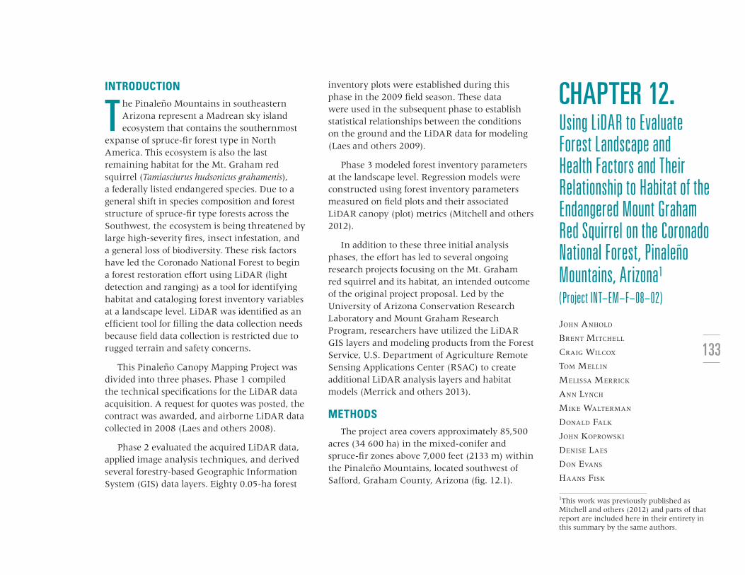
METHODSThe project area covers approximately 85,500

acres (34 600 ha) in the mixed-conifer and spruce-�r zones above 7,000 feet (2133 m) within the Pinaleño Mountains, located southwest of Safford, Graham County, Arizona (�g. 12.1).

1This work was previously published as Mitchell and others (2012) and parts of that report are included here in their entirety in this summary by the same authors.

SECT

ION 3

Ch

apter

12Fo

rest H

ealth

Mon

itorin

g

134

Data collected for this project included airborne LiDAR data and associated �eld plot data. The two datasets were collected with similar dates, and �eld data were collected speci�cally for use with high-resolution LiDAR data.

LiDAR DataHigh pulse-density LiDAR data were

acquired over the Pinaleño Mountains project area September 22–27, 2008. The dataset had a nominal pulse density of ≥3 pulses/m2, >50

percent side lap, and a scan angle within 14 degrees off nadir. The full LiDAR data collection speci�cations and quality assessment can be found in the Phase 2 report by Laes and others (2009).

Field DataField data were collected with the primary

goal of addressing data needs to support LiDAR modeling. Eighty �eld plots were collected in the summer of 2009 based on a 500-m grid.

L iD A R acq uisition

A nalysis area

Figure 12.1—Pinaleño Mountains in southeastern Arizona showing the LiDAR acquisition and forest inventory modeling area represented in a three-dimensional virtual globe environment (Mitchell and others 2012).

135

Plots were 1/20-ha (0.05-ha) �xed plots with a 12.62-m radius. Only 80 of the 200 potential plot locations were sampled due to extreme terrain, one of the primary reasons for the LiDAR project. All plots were permanently monumented and trees tagged.

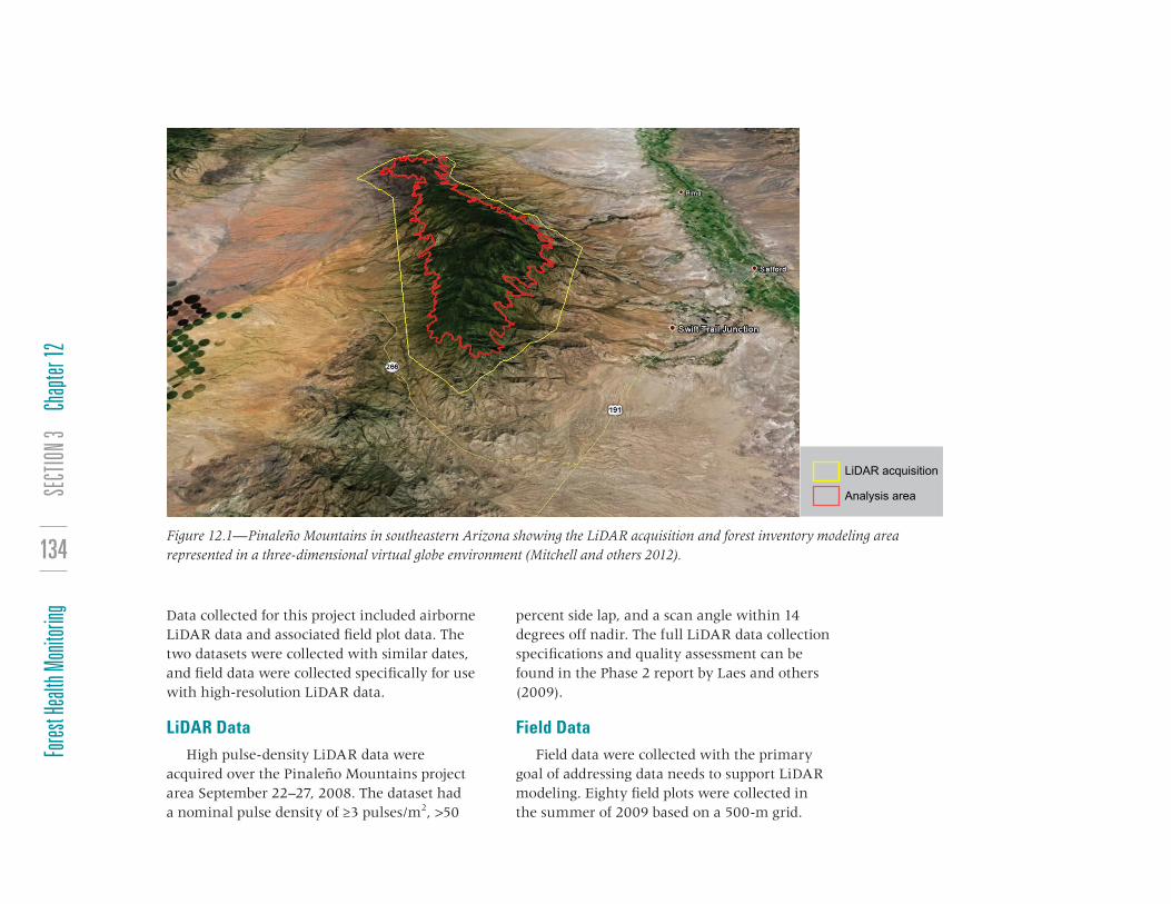
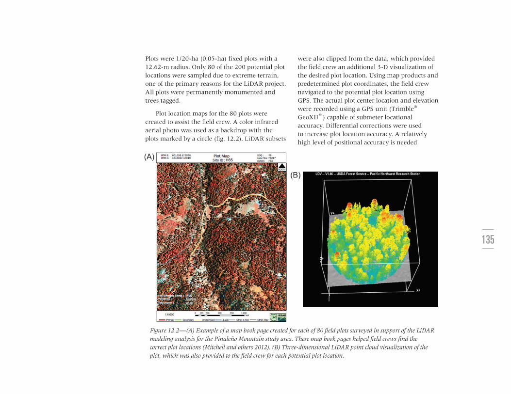
Plot location maps for the 80 plots were created to assist the �eld crew. A color infrared aerial photo was used as a backdrop with the plots marked by a circle (�g. 12.2). LiDAR subsets

were also clipped from the data, which provided the �eld crew an additional 3-D visualization of the desired plot location. Using map products and predetermined plot coordinates, the �eld crew navigated to the potential plot location using GPS. The actual plot center location and elevation were recorded using a GPS unit (Trimble® GeoXH™) capable of submeter locational accuracy. Differential corrections were used to increase plot location accuracy. A relatively high level of positional accuracy is needed

Figure 12.2—(A) Example of a map book page created for each of 80 �eld plots surveyed in support of the LiDAR modeling analysis for the Pinaleño Mountain study area. These map book pages helped �eld crews �nd the correct plot locations (Mitchell and others 2012). (B) Three-dimensional LiDAR point cloud visualization of the plot, which was also provided to the �eld crew for each potential plot location.

(A )

(B )

SECT

ION 3

Ch

apter

12Fo

rest H

ealth

Mon

itorin

g

136

to minimize error and maximize correlation between �eld and LiDAR data in the modeling methodology.

All trees (live or dead) ≥20 cm in diameter at breast height (d.b.h.) and all coarse woody debris (down logs) >20 cm were measured on each plot. To assess smaller trees and small coarse woody fuel, a 1/60-ha wedge-shaped subplot was created within the plot from a random radius bearing. All trees (live or dead) <20 cm in d.b.h. and coarse woody debris <20 cm but ≥5 cm in diameter were measured in the subplot. Three Brown’s fuel transects (Brown 1974) and understory cover transects were used to measure shrub, forbs, grasses, and regeneration. Three photos were collected at each plot location.

The LiDAR and �eld inventory data were then processed and prepared for modeling. The goal of the data processing was to ensure a high level of correspondence between the data sets. Field inventory data were summarized to the plot level [e.g., basal area (BA), stand density index (SDI), average tree height, trees/ha (TPH), and quadratic mean diameter (QMD)] with corresponding metrics from the LiDAR data.

LiDAR predictor variables were generated at the plot scale using FUSION software (McGaughey 2012). The ClipData FUSION command was used to subset the LiDAR data. LiDAR metrics were calculated for each plot’s point cloud using FUSION’s CloudMetrics command. The resulting metrics became the predictor variables for the inventory models.

In summary, the plot level data were used to develop models to estimate the forest inventory variables while LiDAR metrics at the landscape scale were used in subsequent steps to apply the regression models to the entire landscape.

Model DevelopmentPredictive models were created for 23 different

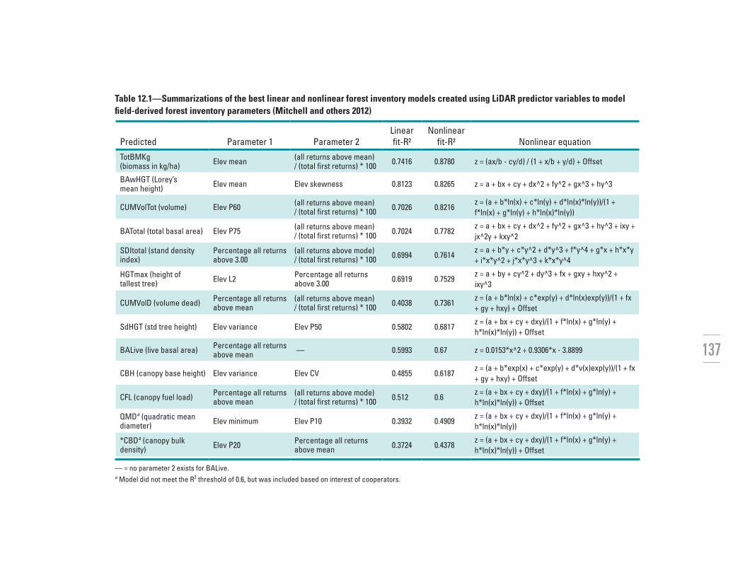
forest and fuel inventory parameters (Mitchell and others 2012). Since all parameters being modeled are represented by continuous values, regression techniques were used to perform the modeling. Nonlinear regression was used to provide adequate predictive functions for each of the modeled parameters. All models created and applied to the landscape, along with the selected LiDAR predictor variables, are displayed in table 12.1.

The modeling process was conducted in �ve principal stages: (1) identify best predictors, (2) create appropriate modeling masks, (3) generate forest inventory models, (4) extrapolation, and (5) validation. To �nd the best linear predictors, a “leave one out” cross validation with a generalized linear regression model was used to �nd the LiDAR-derived parameters that best predicted the plot parameters. Forty LiDAR predictor variables were evaluated for each model. Two selected as additional variables did not contribute to model performance. Once these were selected, a curve-�tting application was used to identify the best nonlinear functions to correlate the LiDAR predictors with the modeled parameters of interest. The �nal models that were regarded as acceptable to apply to the

137

Table 12.1—Summarizations of the best linear and nonlinear forest inventory models created using LiDAR predictor variables to model fi eld-derived forest inventory parameters (Mitchell and others 2012)

Predicted Parameter 1 Parameter 2Linear fi t-R²

Nonlinear fi t-R² Nonlinear equation

TotBMKg (biomass in kg/ha) Elev mean (all returns above mean)

/ (total fi rst returns) * 100 0.7416 0.8780 z = (ax/b - cy/d) / (1 + x/b + y/d) + Offset

BAwHGT (Lorey’s mean height) Elev mean Elev skewness 0.8123 0.8265 z = a + bx + cy + dx^2 + fy^2 + gx^3 + hy^3

CUMVolTot (volume) Elev P60 (all returns above mean) / (total fi rst returns) * 100 0.7026 0.8216

z = (a + b*ln(x) + c*ln(y) + d*ln(x)*ln(y))/(1 + f*ln(x) + g*ln(y) + h*ln(x)*ln(y))

BATotal (total basal area) Elev P75 (all returns above mean) / (total fi rst returns) * 100 0.7024 0.7782

z = a + bx + cy + dx^2 + fy^2 + gx^3 + hy^3 + ixy + jx^2y + kxy^2

SDItotal (stand density index)

Percentage all returns above 3.00

(all returns above mode) / (total fi rst returns) * 100 0.6994 0.7614

z = a + b*y + c*y^2 + d*y^3 + f*y^4 + g*x + h*x*y + i*x*y^2 + j*x*y^3 + k*x*y^4

HGTmax (height of tallest tree) Elev L2 Percentage all returns

above 3.00 0.6919 0.7529z = a + by + cy^2 + dy^3 + fx + gxy + hxy^2 + ixy^3

CUMVolD (volume dead) Percentage all returns above mean

(all returns above mean) / (total fi rst returns) * 100 0.4038 0.7361

z = (a + b*ln(x) + c*exp(y) + d*ln(x)exp(y))/(1 + fx + gy + hxy) + Offset

SdHGT (std tree height) Elev variance Elev P50 0.5802 0.6817z = (a + bx + cy + dxy)/(1 + f*ln(x) + g*ln(y) + h*ln(x)*ln(y)) + Offset

BALive (live basal area) Percentage all returns above mean — 0.5993 0.67 z = 0.0153*x^2 + 0.9306*x - 3.8899

CBH (canopy base height) Elev variance Elev CV 0.4855 0.6187z = (a + b*exp(x) + c*exp(y) + d*v(x)exp(y))/(1 + fx + gy + hxy) + Offset

CFL (canopy fuel load) Percentage all returns above mean

(all returns above mode) / (total fi rst returns) * 100 0.512 0.6

z = (a + bx + cy + dxy)/(1 + f*ln(x) + g*ln(y) + h*ln(x)*ln(y)) + Offset

QMDa (quadratic mean diameter) Elev minimum Elev P10 0.3932 0.4909

z = (a + bx + cy + dxy)/(1 + f*ln(x) + g*ln(y) + h*ln(x)*ln(y))

*CBDa (canopy bulk density) Elev P20 Percentage all returns

above mean 0.3724 0.4378z = (a + bx + cy + dxy)/(1 + f*ln(x) + g*ln(y) + h*ln(x)*ln(y)) + Offset

— = no parameter 2 exists for BALive.a Model did not meet the R2 threshold of 0.6, but was included based on interest of cooperators.

SECT

ION 3

Ch

apter

12Fo

rest H

ealth

Mon

itorin

g

138

landscape based on a smoothness of �t and an R2 value ≥0.6 are displayed in table 12.1. The models for quadratic mean diameter and canopy bulk density were included for further investigation based on interest from the project cooperators even though the models did not meet the R2 threshold.

Some of the forest inventory parameters that performed poorly included downed woody fuels, TPH, and QMD. The poor performance of downed woody fuels models probably re�ects the limitation of LiDAR ground-�ltering models to differentiate between the modeled ground surface and coarse woody debris. TPH and QMD are dif�cult to estimate due to the large variation in tree size. Both QMD and TPH could have bene�ted from a second round of modeling in which trees under a certain diameter class (<5 cm) were excluded from the model. This is typically done in traditional forest inventories where numerous small trees wash out the midstory and overstory characteristics of the unit being measured. Parameters governed by larger tree size, such as BA, SDI, volume, biomass, and Lorey’s mean height, performed well in our study. Lorey’s mean tree height (height of a tree of average BA) holds particular promise (R2 = 0.83) with LiDAR inventories and could be used in a similar fashion as QMD to represent the average tree of a stand. Since all tree heights within the plots were measured, we were able to calculate Lorey’s mean tree height and develop models for this parameter.

LiDAR may be superior to �eld estimates at measuring parameters that are indirectly measured in the �eld, such as crown bulk density, but ascertaining this will require more intensive studies. For example, crown bulk density is estimated from very costly whole tree clipping studies but can be mathematically modeled using more easily measured tree attributes (height, diameter, and species). Clipping studies utilizing LiDAR data may be required to develop better models.

Our models for estimating continuous forest inventory measurements across the LiDAR acquisition area performed poorly in two areas: areas that fell outside the range of plot measurements and thus required the model to extrapolate estimates, and nonforest areas. Predicted data outliers were masked and clipped in the �rst circumstance, and in the latter, nonforested areas were excluded from the modeling process.

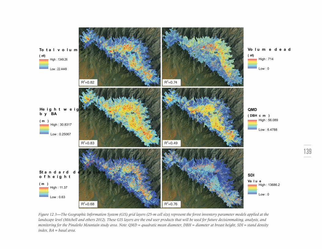
Continuous inventory parameters were created at the landscape scale by applying the derived equations (table 12.1) to the LiDAR GridMetrics layers. Each calculation produced a new grid of cells with 25-m side lengths, each of which spatially represented the estimated forest parameter of interest derived from the LiDAR data (�g. 12.3). These models were validated using local biological, silvicultural, and ecological knowledge of the study area alongside ancillary GIS data and imagery.

139

Figure 12.3—The Geographic Information System (GIS) grid layers (25-m cell size) represent the forest inventory parameter models applied at the landscape level (Mitchell and others 2012). These GIS layers are the end user products that will be used for future decisionmaking, analysis, and monitoring for the Pinaleño Mountain study area. Note: QMD = quadratic mean diameter, DBH = diameter at breast height, SDI = stand density index, BA = basal area.

St a n d a r d d e v i a t i o no f h e i g h t

( m )High : 11.3 7

L ow : 0.63

He i g h t w e i g h t e db y BA

( m )High : 3 0.8 3 17

L ow : 0.25 067

To t a l v o l u m e( m 3)

High : 1349.26

Low : 22.4449

SDIV a l u e

High : 13 68 6.2

L ow : 0

QMD( DBH c m )

High : 5 6.08 9

L ow : 6.47 8 8

V o l u m e d e a d( m 3)

High : 7 14

L ow : 0

R2=0.74

R2=0.83 R2=0.49

R2=0.68 R2=0.76

R2=0.82

SECT

ION 3

Ch

apter

12Fo

rest H

ealth

Mon

itorin

g

140

Since LiDAR technology directly and continuously measures the structural characteristics of the forest vegetation across the landscape, and the modeling methodology used has been replicated and accepted internationally (Means and others 2000, Naesset 2002), we are con�dent that our statistically validated models provide reasonable results representing trends known to exist on the landscape.

CONCLUSIONSThe Pinaleño Canopy Mapping Project

illustrates that forest inventory parameters measured in the �eld can be successfully modeled across the landscape with continuous LiDAR data. Parameters such as biomass (above ground), basal area, Lorey’s mean height, and timber volume appear to lend themselves to this methodology, which is not surprising as they are directly related to tree size and density of vegetation. Our methodology failed to adequately model trees/ha or any of the down woody debris parameters.

The landscape GIS layers are also being used by the Coronado National Forest to create better strategies for managing and conserving the Pinaleño sky island ecosystem. The �rst-order LiDAR derivatives, modeled parameters, and the landscape GIS inventory layers created from this project are currently being incorporated

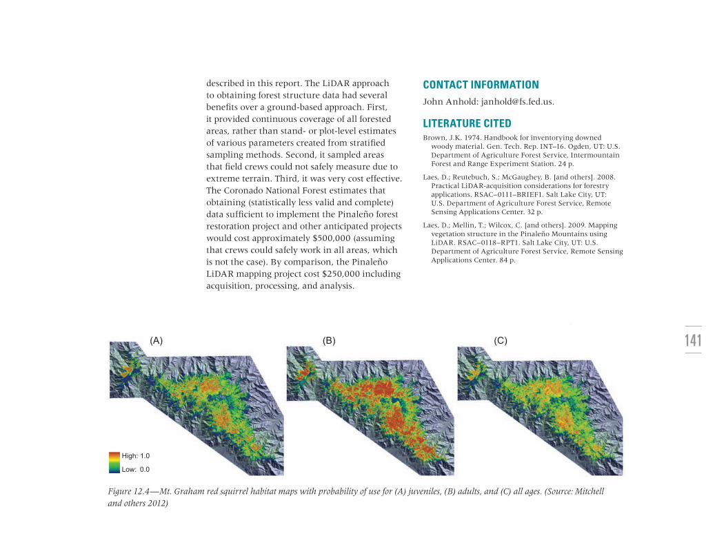
into habitat characterization studies for the Mt. Graham red squirrel. In particular, the University of Arizona Conservation Research Laboratory’s work has utilized the project’s products. The lab’s interests have focused on factors in�uencing natal dispersal movements and habitat selection during adult red squirrel settlement. The researchers are currently testing several hypotheses related to natal habitat preference within mixed conifer forest, decision rules habitat selection, habitat fragmentation, wild�re impacts, and Forest Service restoration treatments and their in�uence on red squirrel dispersal movements and settlement patterns. These studies utilize the Pinaleño LiDAR data in conjunction with other �eld-based measurements to model red squirrel occurrence and settlement, to characterize forest structure, to develop canopy connectivity indices and identify dispersal thresholds, and to identify forest structural features associated with long-term Mt. Graham red squirrel occupancy (Merrick 2014) (�g. 12.4).

This project, from scoping and data acquisition to production of usable GIS layers, took approximately 65 weeks. We have demonstrated that �rst-order LiDAR derivatives, such as canopy height and percent canopy cover, can be used in natural resource management activities without the added cost of �eld data collection and in-depth modeling scenarios

141

described in this report. The LiDAR approach to obtaining forest structure data had several bene�ts over a ground-based approach. First, it provided continuous coverage of all forested areas, rather than stand- or plot-level estimates of various parameters created from strati�ed sampling methods. Second, it sampled areas that �eld crews could not safely measure due to extreme terrain. Third, it was very cost effective. The Coronado National Forest estimates that obtaining (statistically less valid and complete) data suf�cient to implement the Pinaleño forest restoration project and other anticipated projects would cost approximately $500,000 (assuming that crews could safely work in all areas, which is not the case). By comparison, the Pinaleño LiDAR mapping project cost $250,000 including acquisition, processing, and analysis.

CONTACT INFORMATIONJohn Anhold: janhold@fs.fed.us.

LITERATURE CITEDBrown, J.K. 1974. Handbook for inventorying downed

woody material. Gen. Tech. Rep. INT–16. Ogden, UT: U.S. Department of Agriculture Forest Service, Intermountain Forest and Range Experiment Station. 24 p.

Laes, D.; Reutebuch, S.; McGaughey, B. [and others]. 2008. Practical LiDAR-acquisition considerations for forestry applications. RSAC–0111–BRIEF1. Salt Lake City, UT: U.S. Department of Agriculture Forest Service, Remote Sensing Applications Center. 32 p.

Laes, D.; Mellin, T.; Wilcox, C. [and others]. 2009. Mapping vegetation structure in the Pinaleño Mountains using LiDAR. RSAC–0118–RPT1. Salt Lake City, UT: U.S. Department of Agriculture Forest Service, Remote Sensing Applications Center. 84 p.

(B )(A ) (C)

High: 1.0

L ow : 0.0

Figure 12.4—Mt. Graham red squirrel habitat maps with probability of use for (A) juveniles, (B) adults, and (C) all ages. (Source: Mitchell and others 2012)

SECT

ION 3

Ch

apter

12Fo

rest H

ealth

Mon

itorin

g

142

Merrick, M.J. 2014. A new dimension for spatial ecology: LiDAR as a tool for improving wildlife habitat models and fostering collaboration. Remotely Wild: Newsletter of the Spatial Ecology and Telemetry Working Group. The Wildlife Society. Issue 30, Spring: 10-17.

Merrick, M.J.; Koprowski, J.L.; Wilcox, C. 2013. Into the third dimension: bene�ts of incorporating LiDAR into wildlife habitat models. In: Gottfried, G.J.; Gebow, B.S.; Eskew, L.G., eds. Biodiversity and management of the Madrean Archipelago, conference 3. Proceedings RMRS–P–67. Fort Collins, CO: U.S. Department of Agriculture Forest Service, Rocky Mountain Research Station: 389-395.

Mitchell, B.; Walterman, M.; Mellin, T. [and others]. 2012. Mapping vegetation structure in the Pinaleño Mountains using LiDAR—phase 3: forest inventory modeling. RSAC–10007–RPT1. Salt Lake City, UT: U.S. Department of Agriculture Forest Service, Remote Sensing Applications Center. 17 p.

McGaughey, R. 2012. FUSION/LDV: software for LiDAR data analysis and visualization. Version 3.01. Seattle, WA: U.S. Department of Agriculture Forest Service, Paci�c Northwest Research Station. http://forsys.cfr.washington.edu/fusion/fusionlatest.html. [Date accessed: April 2, 2012].

Means, J.E.; Acker, S.A.; Fitt, B.J. [and others]. 2000. Predicting forest stand characteristics with airborne scanning LiDAR. Photogrammetric Engineering and Remote Sensing. 66(11): 1367-1371.

Naesset, E. 2002. Predicting forest stand characteristics with airborne scanning laser using a practical two-stage procedure and �eld data. Remote Sensing of Environment. 80: 88-99.

Forest Health Monitoring: National Status, Trends, and Analysis 2014

Editors Kevin M. Potter Barbara L. Conkling

United States Department of Agriculture

Forest ServiceResearch & DevelopmentSouthern Research StationGeneral Technical Report SRS-209

July 2015Southern Research Station

200 W.T. Weaver Blvd.Asheville, NC 28804

www.srs.fs.usda.gov

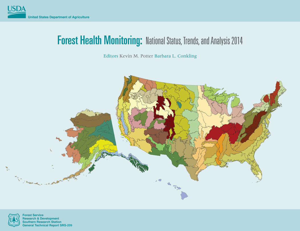
Front cover map: Ecoregion provinces and ecoregion sections for the conterminous United States (Cleland and others 2007) and for Alaska (Nowacki and Brock 1995).

Back cover map: Forest cover (green) backdrop derived from Moderate Resolution Imaging Spectroradiometer (MODIS) satellite imagery by the U.S. Forest Service Remote Sensing Applications Center.

DISCLAIMER

The use of trade or �rm names in this publication is for reader information and does not imply endorsement by the U.S. Department of Agriculture of any product or service.

PESTICIDE PRECAUTIONARY STATEMENT

This publication reports research involving pesticides. It does not contain recommendations for their use, nor does it imply that the uses discussed here have been registered. All uses of pesticides must be registered

by appropriate State and/or Federal agencies before they can be recommended.

CAUTION: Pesticides can be injurious to humans, domestic animals, desirable plants, and �sh or other wildlife—if they are not handled or applied properly. Use all pesticides selectively and carefully.

Follow recommended practices for the disposal of surplus pesticides and pesticide containers.

Forest Health Monitoring: National Status, Trends, and Analysis 2014

Editors

Kevin M. Potter, Research Associate Professor, North Carolina State University, Department of Forestry and Environmental Resources, Raleigh, NC 27695

Barbara L. Conkling, Research Assistant Professor, North Carolina State University, Department of Forestry and Environmental Resources, Raleigh, NC 27695

ii

The annual national report of the Forest Health Monitoring (FHM) Program of the Forest Service, U.S. Department of

Agriculture, presents forest health status and trends from a national or multi-State regional perspective using a variety of sources, introduces new techniques for analyzing forest health data, and summarizes results of recently completed Evaluation Monitoring projects funded through the FHM national program. In this 14th edition in a series of annual reports, survey data are used to identify geographic patterns of forest insect and disease activity. Satellite data are employed to detect geographic patterns of forest �re occurrence. Recent drought conditions

are compared across the conterminous United States. Data collected by the Forest Inventory and Analysis (FIA) Program are employed to detect regional differences in tree mortality. Results of a national insect and disease forest risk assessment, including maps, are presented. Using FIA and national land cover data, decline of intact forest is assessed by forest type and ownership. Ten recently completed Evaluation Monitoring projects are summarized, addressing forest health concerns at smaller scales.

Keywords—Change detection, drought, �re, forest health, forest insects and disease, fragmentation, risk assessment, tree mortality.

ABSTRACT

Potter, Kevin M.; Conkling, Barbara L., eds. 2015. Forest Health Monitoring: national status, trends, and analysis 2014. Gen. Tech. Rep. SRS-209. Asheville, NC: U.S. Department of Agriculture Forest Service, Southern Research Station. 190 p.

The annual national report of the Forest Health Monitoring (FHM) Program of the Forest Service, U.S. Department of Agriculture, presents forest health status and trends from a national or multi-State regional perspective using a variety of sources, introduces new techniques for analyzing forest health data, and summarizes results of recently completed Evaluation Monitoring projects funded through the FHM national program. In this 14th edition in a series of annual reports, survey data are used to identify geographic patterns of forest insect and disease activity. Satellite data are employed to detect geographic patterns of forest �re occurrence. Recent drought conditions are compared across the conterminous United States. Data collected by the Forest Inventory and Analysis (FIA) Program are employed to detect regional differences in tree mortality. Results of a national insect and disease forest risk assessment, including maps, are presented. Using FIA and national land cover data, decline of intact forest is assessed by forest type and ownership. Ten recently completed Evaluation Monitoring projects are summarized, addressing forest health concerns at smaller scales.

Keywords—Change detection, drought, �re, forest health, forest insects and disease, fragmentation, risk assessment, tree mortality.

Scan this code to submit your feedback, or go to www.srs.fs.usda.gov/pubeval

You may request a copy of this publication by email at pubrequest@fs.fed.us.

In accordance with Federal civil rights law and U.S. Department of Agriculture (USDA) civil rights regulations and policies, the USDA, its

Agencies, offices, and employees, and institutions participating in or administering USDA programs are prohibited from discriminating based on race, color, national origin, religion, sex, gender identity (including gender expression), sexual orientation, disability, age, marital status, family/parental status, income derived from a public assistance program, political beliefs, or reprisal or retaliation for prior civil rights activity, in any program or activity conducted or funded by USDA (not all bases apply to all programs). Remedies and complaint filing deadlines vary by program or incident.

Persons with disabilities who require alternative means of communication for program information (e.g., Braille, large print, audiotape, American Sign Language, etc.) should contact the responsible Agency or USDA’s TARGET Center at (202) 720-2600 (voice and TTY) or contact USDA through the Federal Relay Service at (800) 877-8339. Additionally, program information may be made available in languages other than English.

To file a program discrimination complaint, complete the USDA Program Discrimination Complaint Form, AD-3027, found online at http://www.ascr.usda.gov/complaint_filing_cust.

html and at any USDA office or write a letter addressed to USDA and provide in the letter all of the information requested in the form. To request a copy of the complaint form, call (866) 632-9992. Submit your completed form or letter to USDA by: (1) mail: U.S. Department of Agriculture, Officeof the Assistant Secretary for Civil Rights, 1400Independence Avenue, SW, Washington, D.C.20250-9410; (2) fax: (202) 690-7442; or (3) email:program.intake@usda.gov.

USDA is an equal opportunity provider, employer, and lender.