interpreters and virtual machines · an interpreter is a program that executes another program,...
TRANSCRIPT

Interpreters and virtual machines
Advanced Compiler Construction Michel Schinz — 2016–04–28

Interpreters
InterpretersAn interpreter is a program that executes another program, represented as some kind of data-structure. Common program representations include:
– raw text (source code), – trees (AST of the program), – linear sequences of instructions.
Interpreters enable the execution of a program without requiring its compilation to native code. They simplify the implementation of programming languages and — on modern hardware — are efficient enough for many tasks.
Text-based interpreters
Text-based interpreters directly interpret the textual source of the program. They are very seldom used, except for trivial languages where every expression is evaluated at most once — i.e. languages without loops or functions. Plausible example: a calculator program, which evaluates arithmetic expressions while parsing them.
Tree-based interpreters
Tree-based interpreters walk over the abstract syntax tree of the program to interpret it. Their advantage compared to string-based interpreters is that parsing — and name/type analysis, if applicable — is done only once. Plausible example: a graphing program, which has to repeatedly evaluate a function supplied by the user to plot it. All the interpreters included in the L3 compiler are also tree-based.

Virtual machines
Virtual machinesVirtual machines resemble real processors, but are implemented in software. They accept as input a program composed of a sequence of instructions. Virtual machines often provide more than the simple interpretation of programs: they also abstract the underlying system by managing memory, threads, and sometimes I/O. Perhaps surprisingly, virtual machines are a very old concept, dating back to ~1950. They have been — and still are — used in the implementation of many important languages, like SmallTalk, Lisp, Forth, Pascal, and more recently Java and C#.
Why virtual machines?
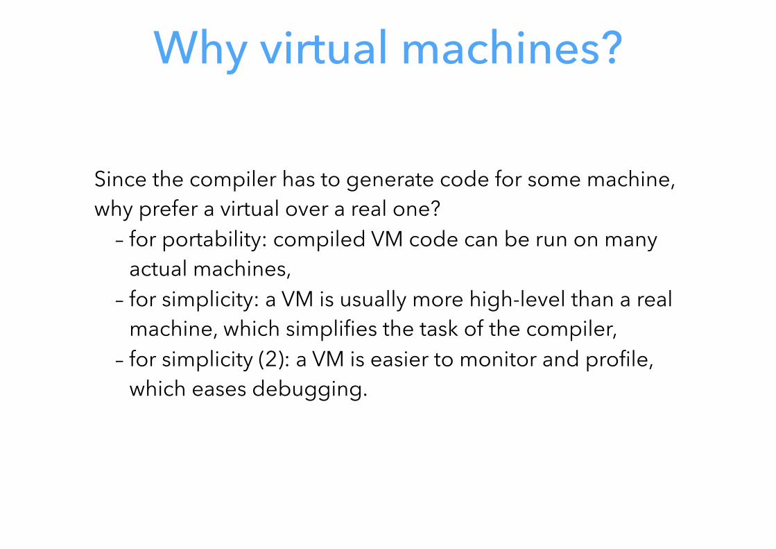
Since the compiler has to generate code for some machine, why prefer a virtual over a real one?
– for portability: compiled VM code can be run on many actual machines,
– for simplicity: a VM is usually more high-level than a real machine, which simplifies the task of the compiler,
– for simplicity (2): a VM is easier to monitor and profile, which eases debugging.
Virtual machines drawbacks
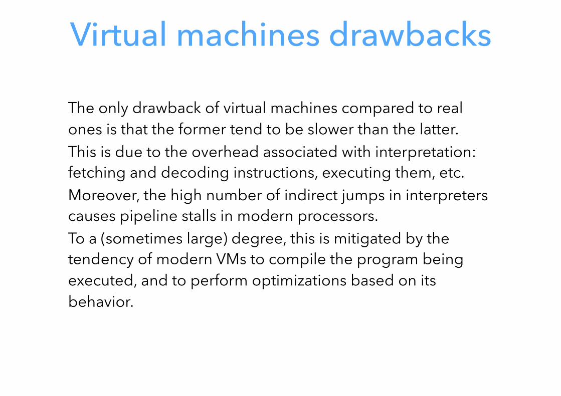
The only drawback of virtual machines compared to real ones is that the former tend to be slower than the latter. This is due to the overhead associated with interpretation: fetching and decoding instructions, executing them, etc. Moreover, the high number of indirect jumps in interpreters causes pipeline stalls in modern processors. To a (sometimes large) degree, this is mitigated by the tendency of modern VMs to compile the program being executed, and to perform optimizations based on its behavior.
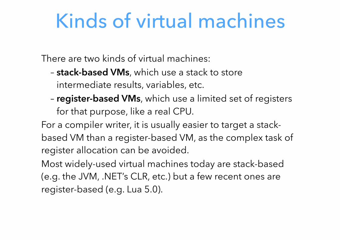
Kinds of virtual machinesThere are two kinds of virtual machines:
– stack-based VMs, which use a stack to store intermediate results, variables, etc.
– register-based VMs, which use a limited set of registers for that purpose, like a real CPU.
For a compiler writer, it is usually easier to target a stack-based VM than a register-based VM, as the complex task of register allocation can be avoided. Most widely-used virtual machines today are stack-based (e.g. the JVM, .NET’s CLR, etc.) but a few recent ones are register-based (e.g. Lua 5.0).
Virtual machine input
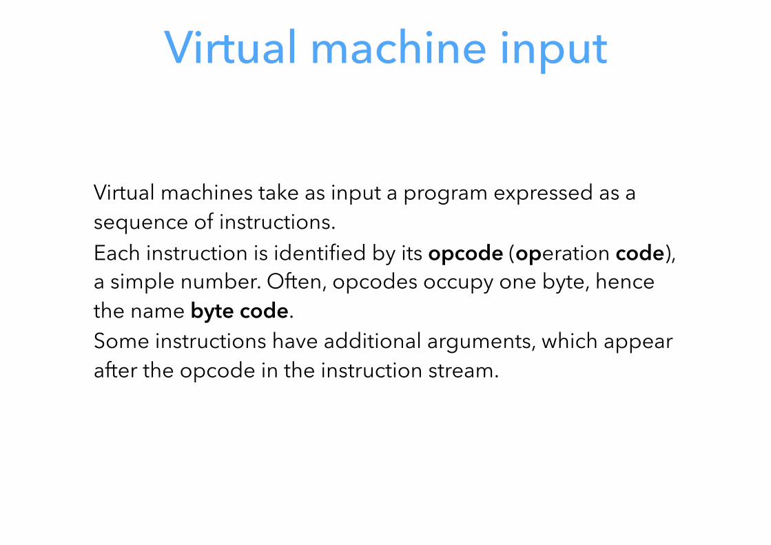
Virtual machines take as input a program expressed as a sequence of instructions. Each instruction is identified by its opcode (operation code), a simple number. Often, opcodes occupy one byte, hence the name byte code. Some instructions have additional arguments, which appear after the opcode in the instruction stream.
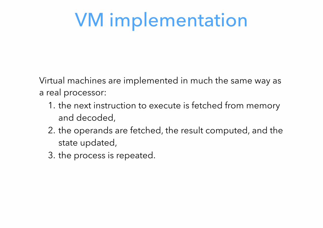
VM implementation
Virtual machines are implemented in much the same way as a real processor:
1. the next instruction to execute is fetched from memory and decoded,
2. the operands are fetched, the result computed, and the state updated,
3. the process is repeated.
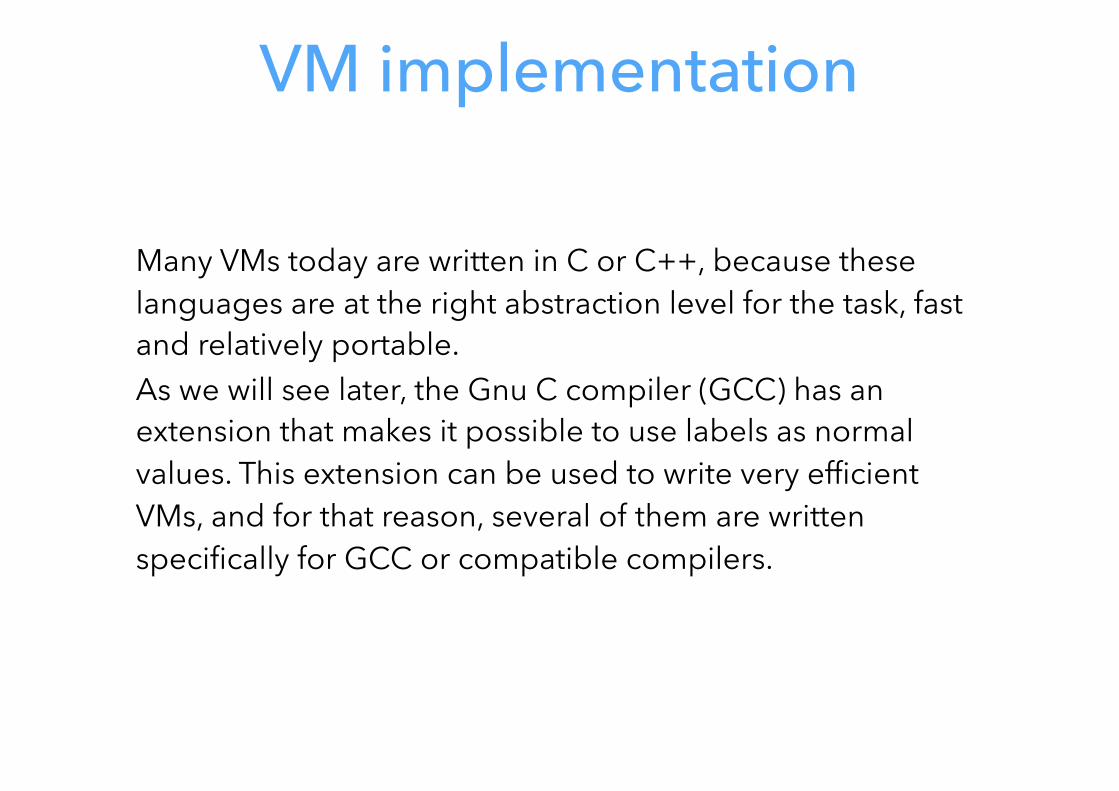
VM implementation
Many VMs today are written in C or C++, because these languages are at the right abstraction level for the task, fast and relatively portable. As we will see later, the Gnu C compiler (GCC) has an extension that makes it possible to use labels as normal values. This extension can be used to write very efficient VMs, and for that reason, several of them are written specifically for GCC or compatible compilers.
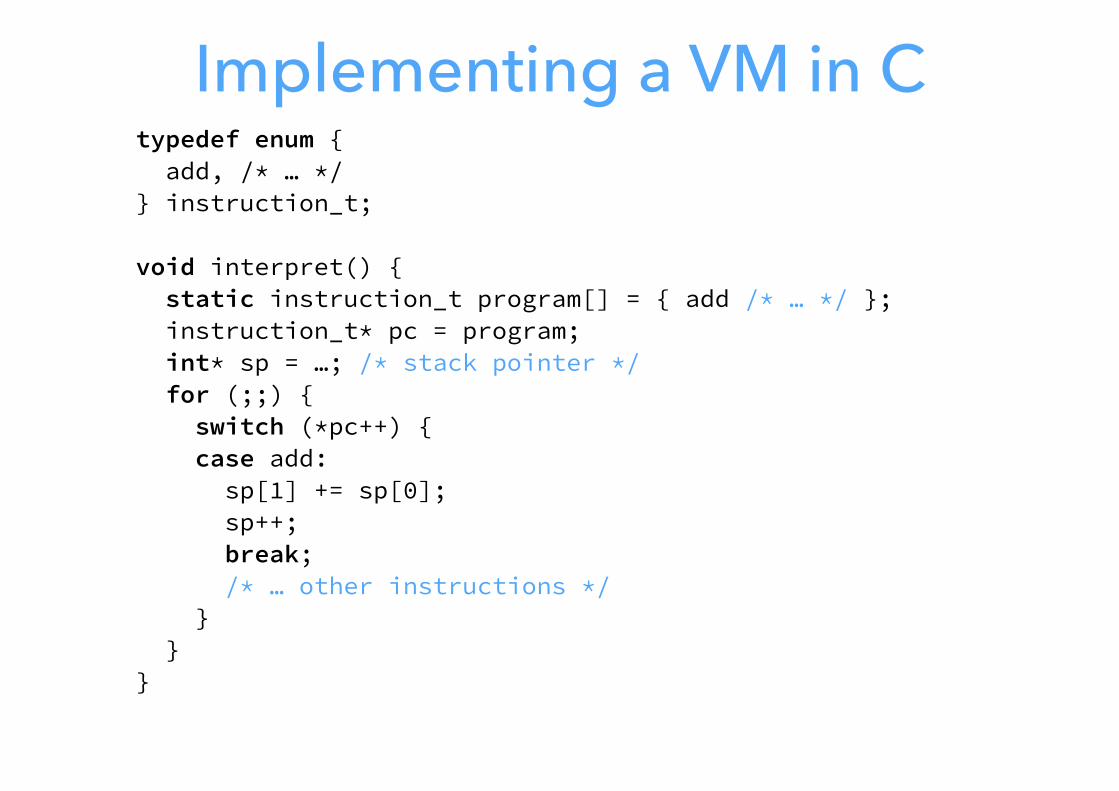
Implementing a VM in Ctypedef enum { add, /* … */ } instruction_t; void interpret() { static instruction_t program[] = { add /* … */ }; instruction_t* pc = program; int* sp = …; /* stack pointer */ for (;;) { switch (*pc++) { case add: sp[1] += sp[0]; sp++; break; /* … other instructions */ } }}
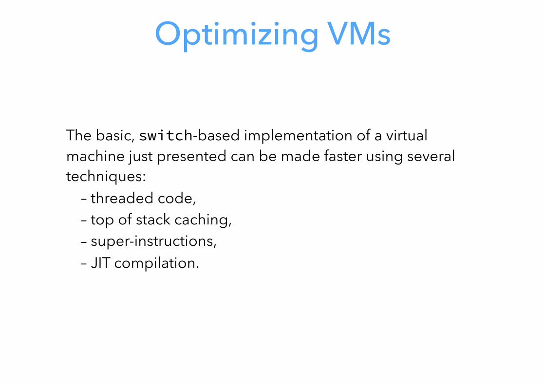
Optimizing VMs
The basic, switch-based implementation of a virtual machine just presented can be made faster using several techniques:
– threaded code, – top of stack caching, – super-instructions, – JIT compilation.
Threaded code
Threaded code
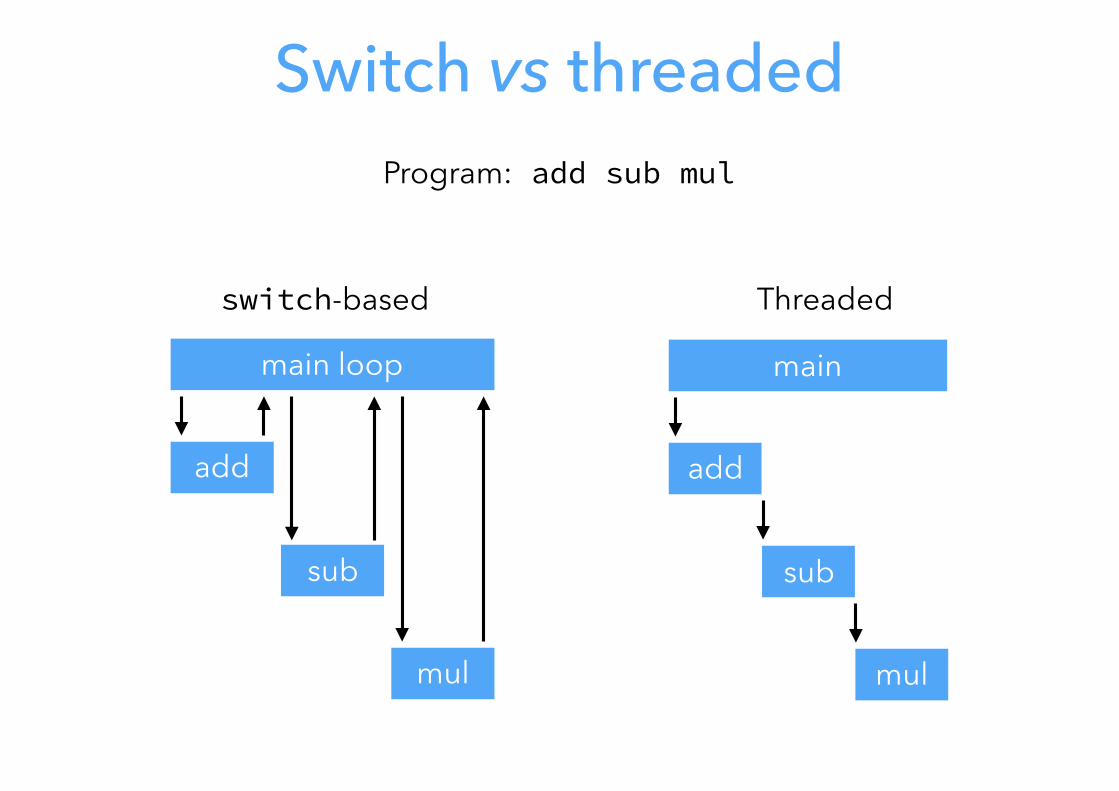
In a switch-based interpreter, each instruction requires two jumps:
– one indirect jump to the branch handling the current instruction,
– one direct jump from there to the main loop. It would be better to avoid the second one, by jumping directly to the code handling the next instruction. This is the idea of threaded code.
Switch vs threaded
switch-based
main loop
add
sub
mul
Threaded
main
add
sub
mul
Program: add sub mul
Implementing threaded code
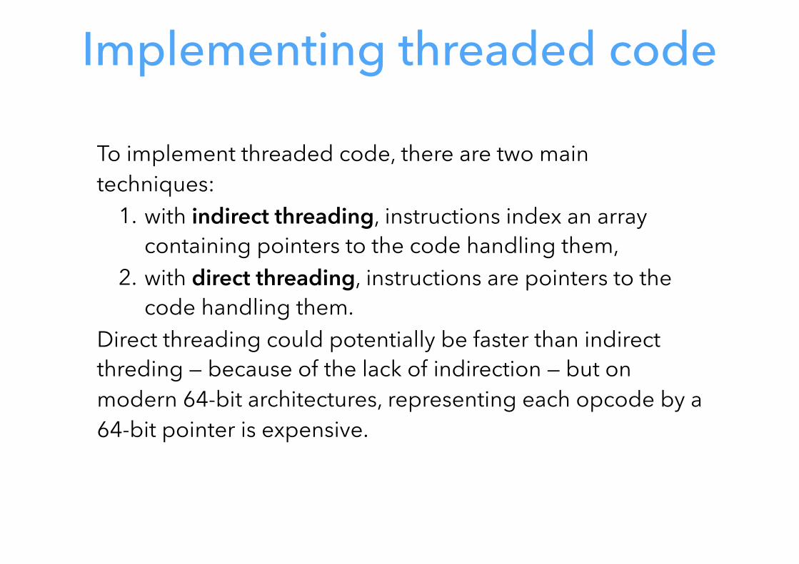
To implement threaded code, there are two main techniques:
1. with indirect threading, instructions index an array containing pointers to the code handling them,
2. with direct threading, instructions are pointers to the code handling them.
Direct threading could potentially be faster than indirect threding — because of the lack of indirection — but on modern 64-bit architectures, representing each opcode by a 64-bit pointer is expensive.
Threaded code in C
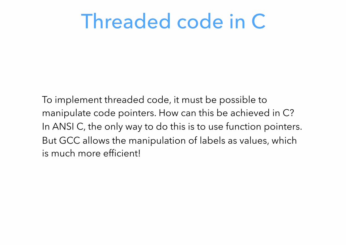
To implement threaded code, it must be possible to manipulate code pointers. How can this be achieved in C? In ANSI C, the only way to do this is to use function pointers. But GCC allows the manipulation of labels as values, which is much more efficient!
Direct threading in ANSI C
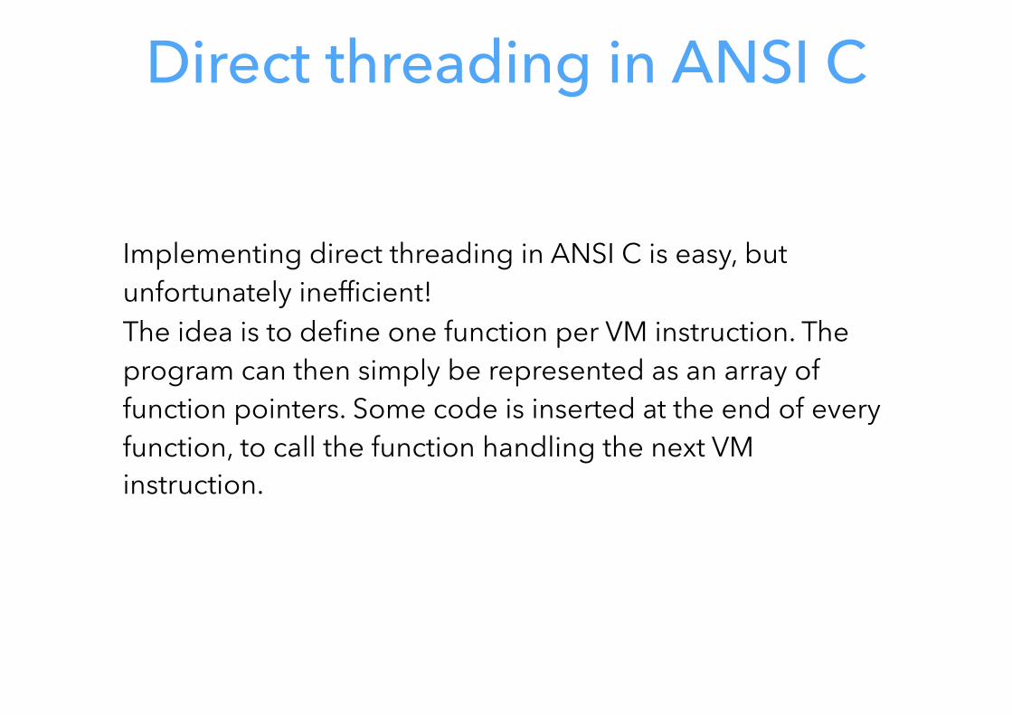
Implementing direct threading in ANSI C is easy, but unfortunately inefficient! The idea is to define one function per VM instruction. The program can then simply be represented as an array of function pointers. Some code is inserted at the end of every function, to call the function handling the next VM instruction.
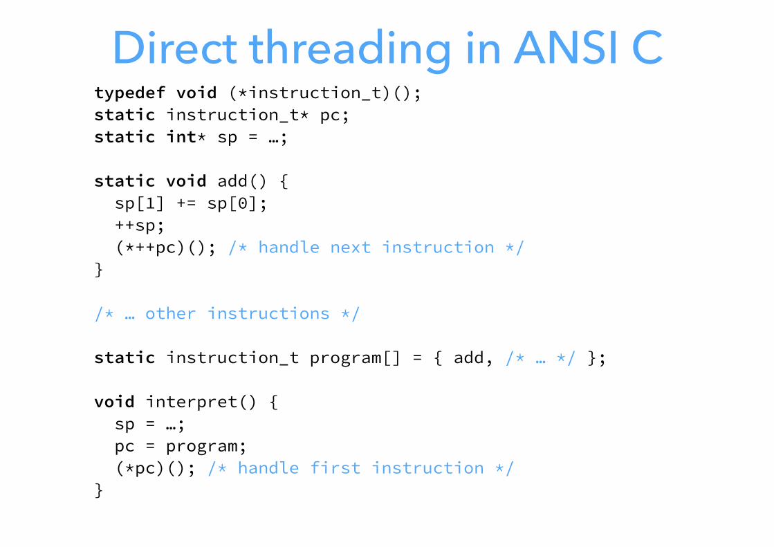
Direct threading in ANSI Ctypedef void (*instruction_t)(); static instruction_t* pc; static int* sp = …; static void add() { sp[1] += sp[0]; ++sp; (*++pc)(); /* handle next instruction */}/* … other instructions */ static instruction_t program[] = { add, /* … */ };void interpret() { sp = …; pc = program; (*pc)(); /* handle first instruction */ }
Direct threading in ANSI C
This implementation of direct threading in ANSI C has a major problem: it leads to stack overflow very quickly, unless the compiler implements tail call elimination. In our interpreter, the function call appearing at the end of add — and all other functions implementing VM instructions — is a tail call and should be optimized. While recent versions of GCC do full tail call elimination, not all compilers do. With such compilers, the only option is to eliminate tail calls by hand, e.g. using trampolines.
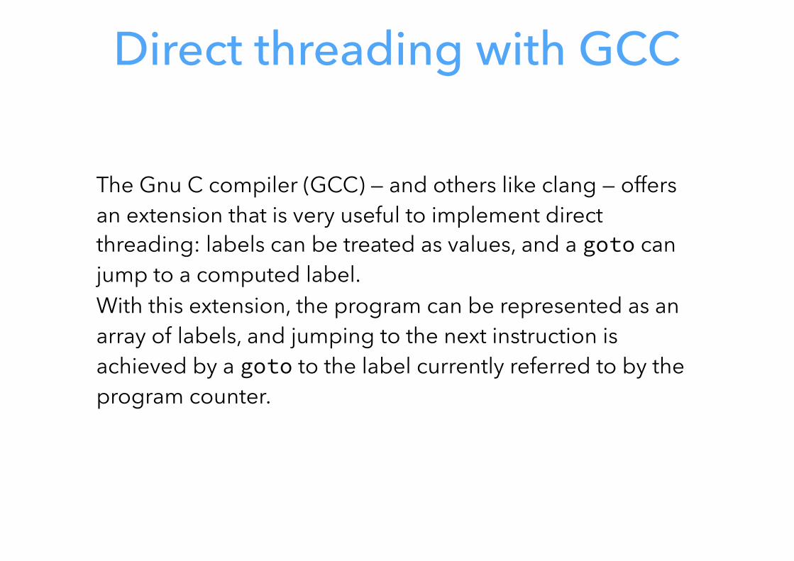
Direct threading with GCC
The Gnu C compiler (GCC) — and others like clang — offers an extension that is very useful to implement direct threading: labels can be treated as values, and a goto can jump to a computed label. With this extension, the program can be represented as an array of labels, and jumping to the next instruction is achieved by a goto to the label currently referred to by the program counter.
Direct threading with GCCvoid interpret() { void* program[] = { &&l_add, /* … */ }; int* sp = …; void** pc = program; goto **pc; /* jump to first instruction */ l_add: sp[1] += sp[0]; ++sp; goto **(++pc); /* jump to next instruction */ /* … other instructions */ }
label as value
computed goto
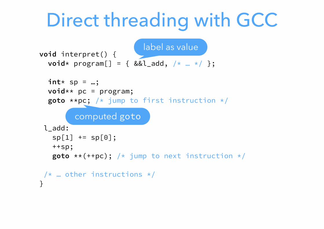
Threading benchmarkThe benchmark below compares several versions of a small interpreter measured while interpreting 500’000’000 iterations of a simple loop. The code was compiled using clang v503.0.38 with full optimizations, and run on an Intel Core i5. The normalized times are presented below.
switch-based
trampoline
no trampoline (with TCE)
labels as values
0 0.5 1 1.5 2
0.56
1.67
1.74
1

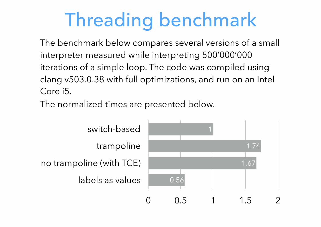
Top-of-stack caching

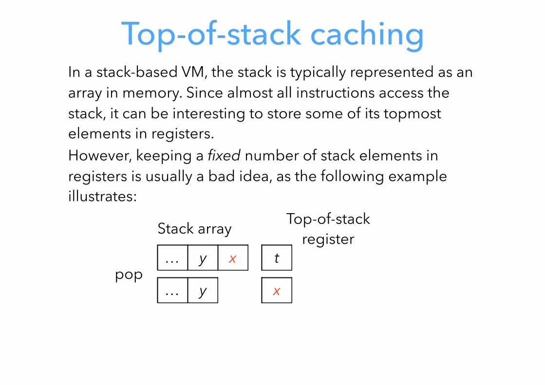
Top-of-stack cachingIn a stack-based VM, the stack is typically represented as an array in memory. Since almost all instructions access the stack, it can be interesting to store some of its topmost elements in registers. However, keeping a fixed number of stack elements in registers is usually a bad idea, as the following example illustrates:
t
Stack array Top-of-stack register
… y x
Top-of-stack cachingIn a stack-based VM, the stack is typically represented as an array in memory. Since almost all instructions access the stack, it can be interesting to store some of its topmost elements in registers. However, keeping a fixed number of stack elements in registers is usually a bad idea, as the following example illustrates:
t
Stack array Top-of-stack register
pop… y x
Top-of-stack cachingIn a stack-based VM, the stack is typically represented as an array in memory. Since almost all instructions access the stack, it can be interesting to store some of its topmost elements in registers. However, keeping a fixed number of stack elements in registers is usually a bad idea, as the following example illustrates:
t
Stack array Top-of-stack register
xpop
… y x
… y
Top-of-stack cachingIn a stack-based VM, the stack is typically represented as an array in memory. Since almost all instructions access the stack, it can be interesting to store some of its topmost elements in registers. However, keeping a fixed number of stack elements in registers is usually a bad idea, as the following example illustrates:
t
Stack array Top-of-stack register
xpop
push u
… y x
… y

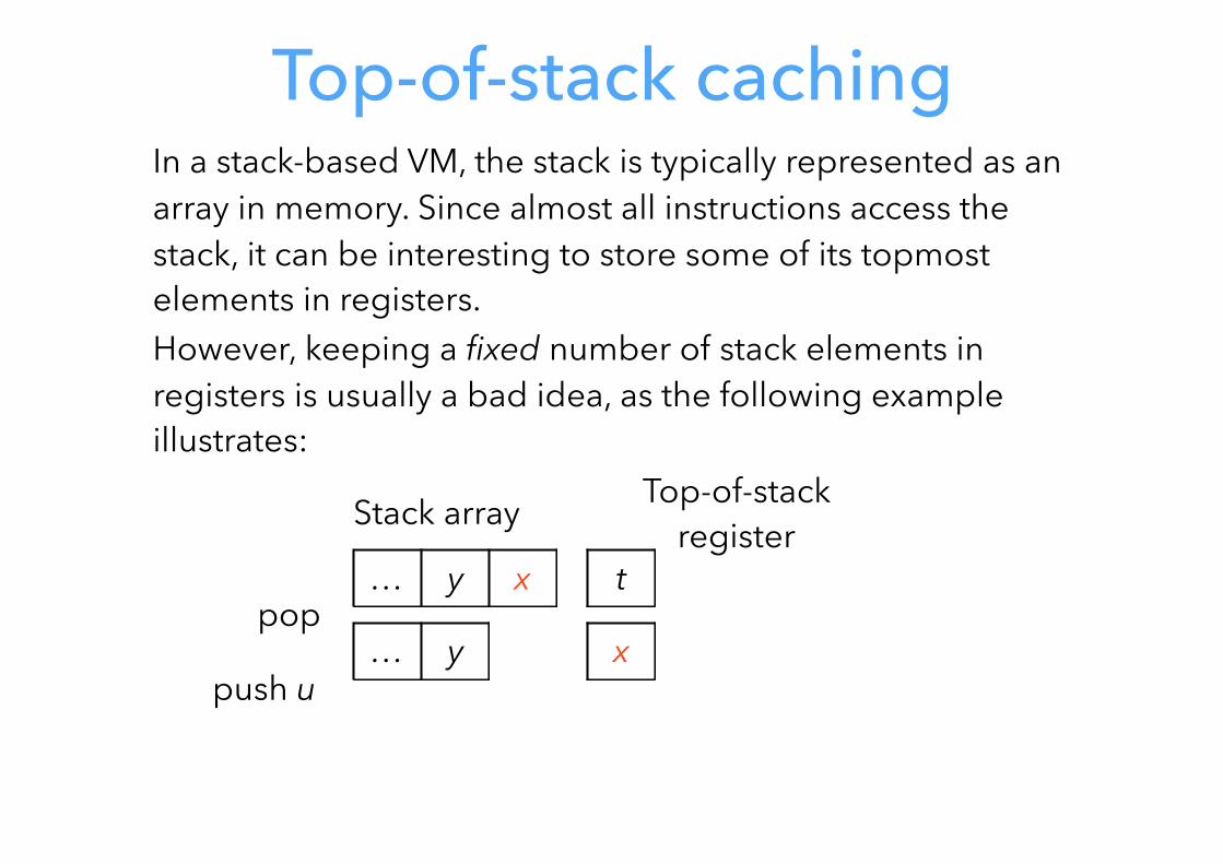
Top-of-stack cachingIn a stack-based VM, the stack is typically represented as an array in memory. Since almost all instructions access the stack, it can be interesting to store some of its topmost elements in registers. However, keeping a fixed number of stack elements in registers is usually a bad idea, as the following example illustrates:
t
Stack array Top-of-stack register
x
u
pop
push u
… y x
… y x
… y

Top-of-stack cachingIn a stack-based VM, the stack is typically represented as an array in memory. Since almost all instructions access the stack, it can be interesting to store some of its topmost elements in registers. However, keeping a fixed number of stack elements in registers is usually a bad idea, as the following example illustrates:
t
Stack array Top-of-stack register
x
u
pop
push u
… y x
… y x
… yx moves
around unnecessarily
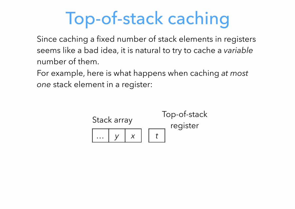
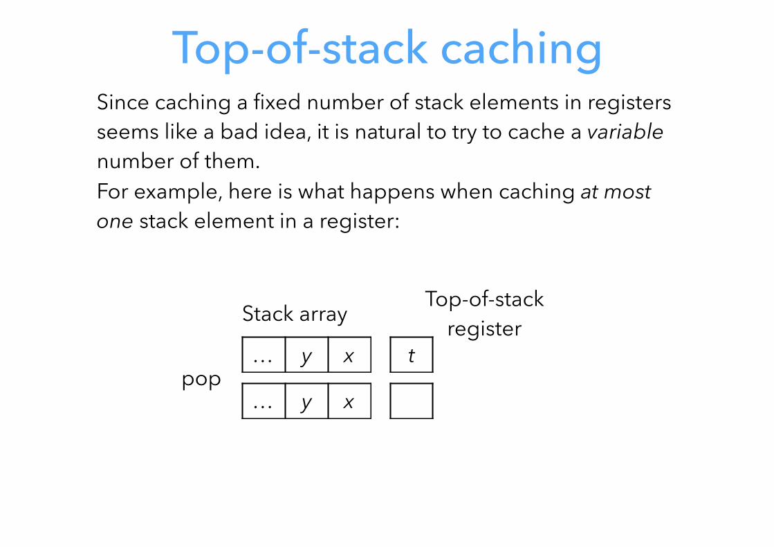
Top-of-stack cachingSince caching a fixed number of stack elements in registers seems like a bad idea, it is natural to try to cache a variable number of them. For example, here is what happens when caching at most one stack element in a register:
t
Stack array Top-of-stack register
… y x
Top-of-stack cachingSince caching a fixed number of stack elements in registers seems like a bad idea, it is natural to try to cache a variable number of them. For example, here is what happens when caching at most one stack element in a register:
t
Stack array Top-of-stack register
pop… y x
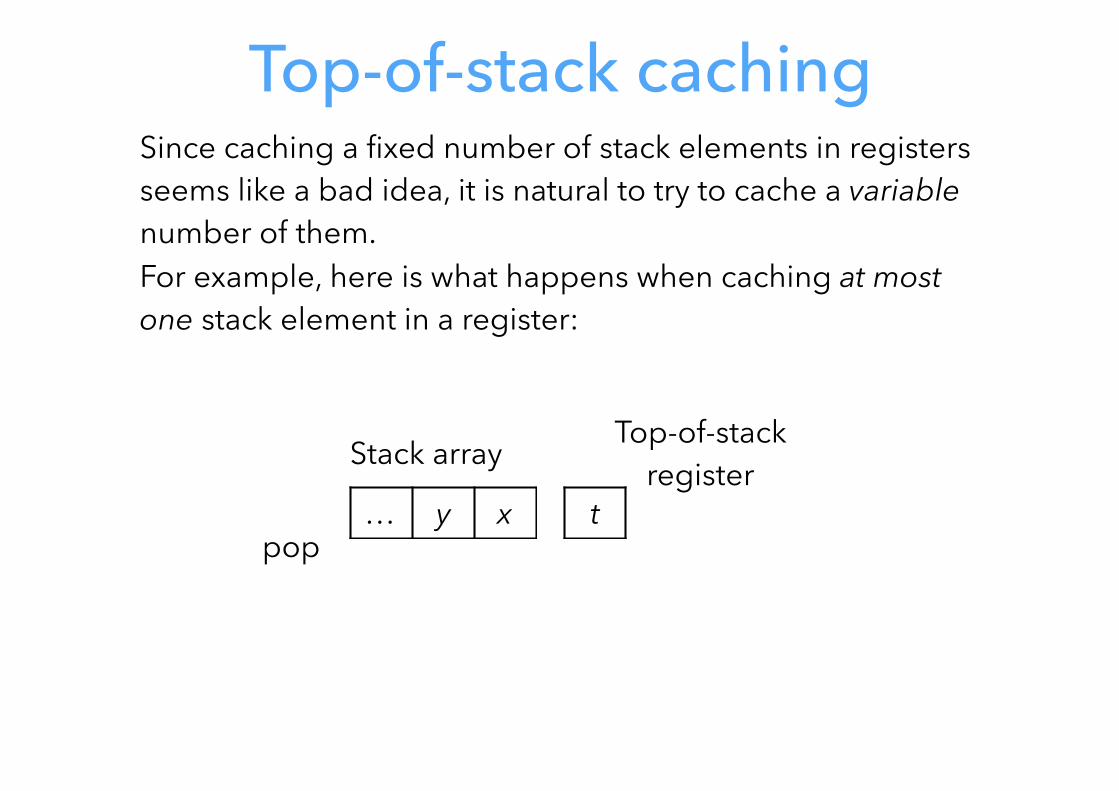
Top-of-stack cachingSince caching a fixed number of stack elements in registers seems like a bad idea, it is natural to try to cache a variable number of them. For example, here is what happens when caching at most one stack element in a register:
t
Stack array Top-of-stack register
pop… y x
… y x
Top-of-stack cachingSince caching a fixed number of stack elements in registers seems like a bad idea, it is natural to try to cache a variable number of them. For example, here is what happens when caching at most one stack element in a register:
t
Stack array Top-of-stack register
pop
push u
… y x
… y x
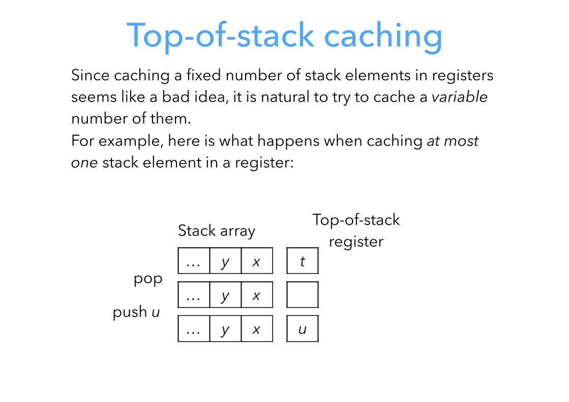
Top-of-stack cachingSince caching a fixed number of stack elements in registers seems like a bad idea, it is natural to try to cache a variable number of them. For example, here is what happens when caching at most one stack element in a register:
t
Stack array Top-of-stack register
u
pop
push u
… y x
… y x
… y x
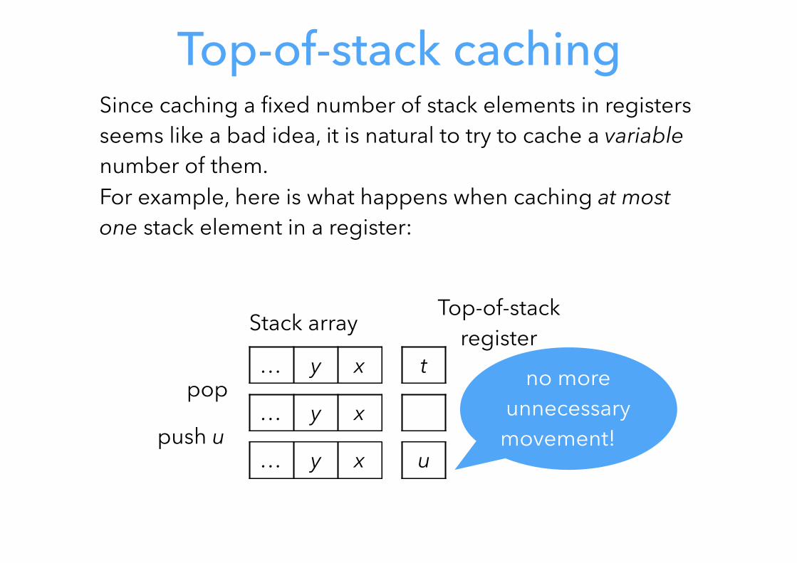
Top-of-stack cachingSince caching a fixed number of stack elements in registers seems like a bad idea, it is natural to try to cache a variable number of them. For example, here is what happens when caching at most one stack element in a register:
t
Stack array Top-of-stack register
u
pop
push u
… y x
… y x
… y xno more
unnecessary movement!
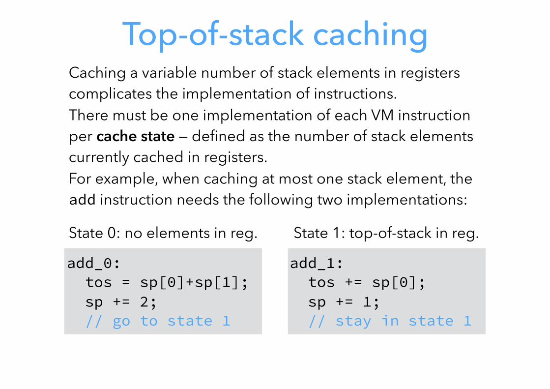
Top-of-stack cachingCaching a variable number of stack elements in registers complicates the implementation of instructions. There must be one implementation of each VM instruction per cache state — defined as the number of stack elements currently cached in registers. For example, when caching at most one stack element, the add instruction needs the following two implementations:
add_0: tos = sp[0]+sp[1]; sp += 2; // go to state 1
add_1: tos += sp[0]; sp += 1; // stay in state 1
State 0: no elements in reg. State 1: top-of-stack in reg.
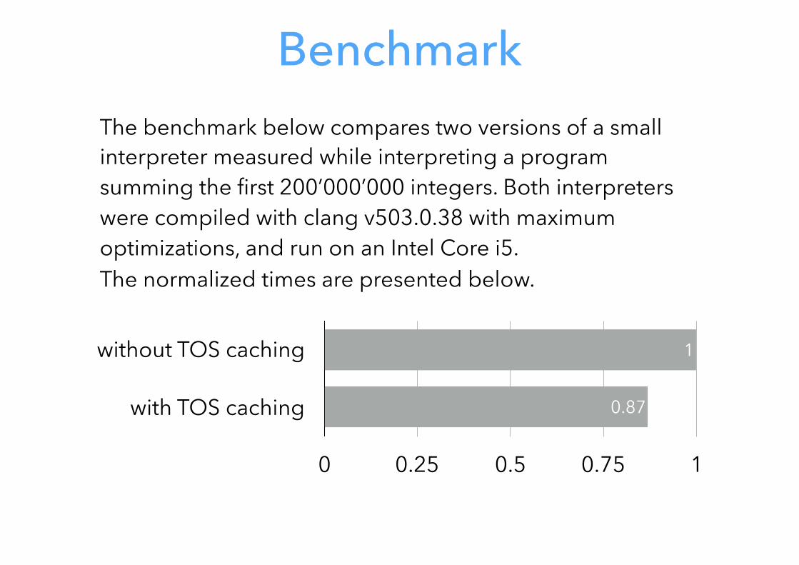
Benchmark
without TOS caching
with TOS caching
0 0.25 0.5 0.75 1
0.87
1
The benchmark below compares two versions of a small interpreter measured while interpreting a program summing the first 200’000’000 integers. Both interpreters were compiled with clang v503.0.38 with maximum optimizations, and run on an Intel Core i5. The normalized times are presented below.
Super-instructions
Static super-instructions
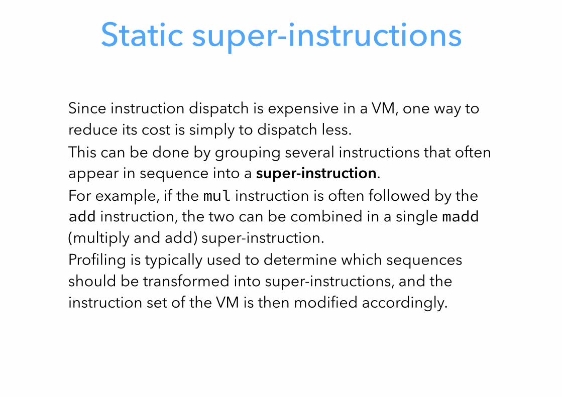
Since instruction dispatch is expensive in a VM, one way to reduce its cost is simply to dispatch less. This can be done by grouping several instructions that often appear in sequence into a super-instruction. For example, if the mul instruction is often followed by the add instruction, the two can be combined in a single madd (multiply and add) super-instruction. Profiling is typically used to determine which sequences should be transformed into super-instructions, and the instruction set of the VM is then modified accordingly.
Dynamic super-instructions
It is also possible to generate super-instructions at run time, to adapt them to the program being run. This is the idea behind dynamic super-instructions. This technique can be pushed to its limits, by generating one super-instruction for every basic block of the program! This effectively transform all basic blocks into single (super-)instructions.
L3VM
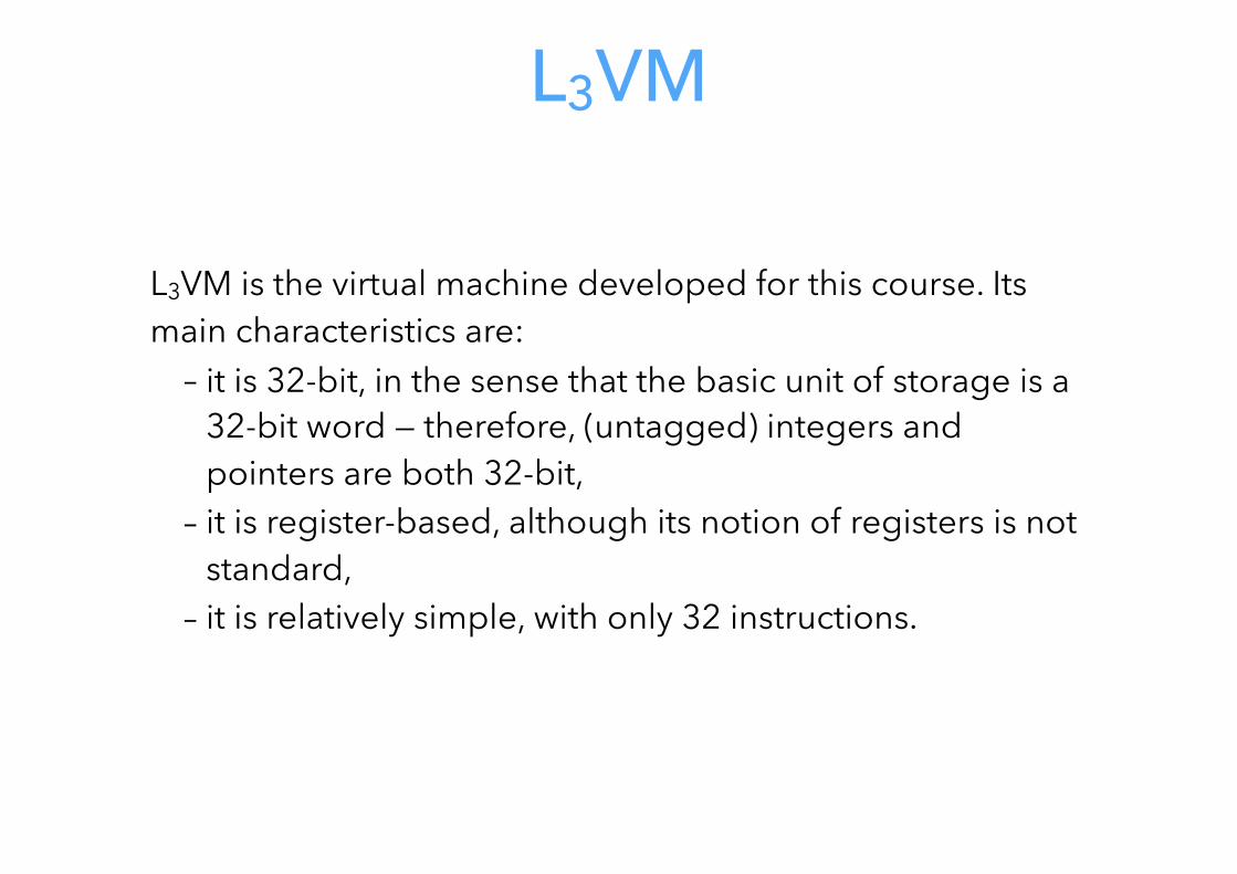
L3VM
L3VM is the virtual machine developed for this course. Its main characteristics are:
– it is 32-bit, in the sense that the basic unit of storage is a 32-bit word — therefore, (untagged) integers and pointers are both 32-bit,
– it is register-based, although its notion of registers is not standard,
– it is relatively simple, with only 32 instructions.
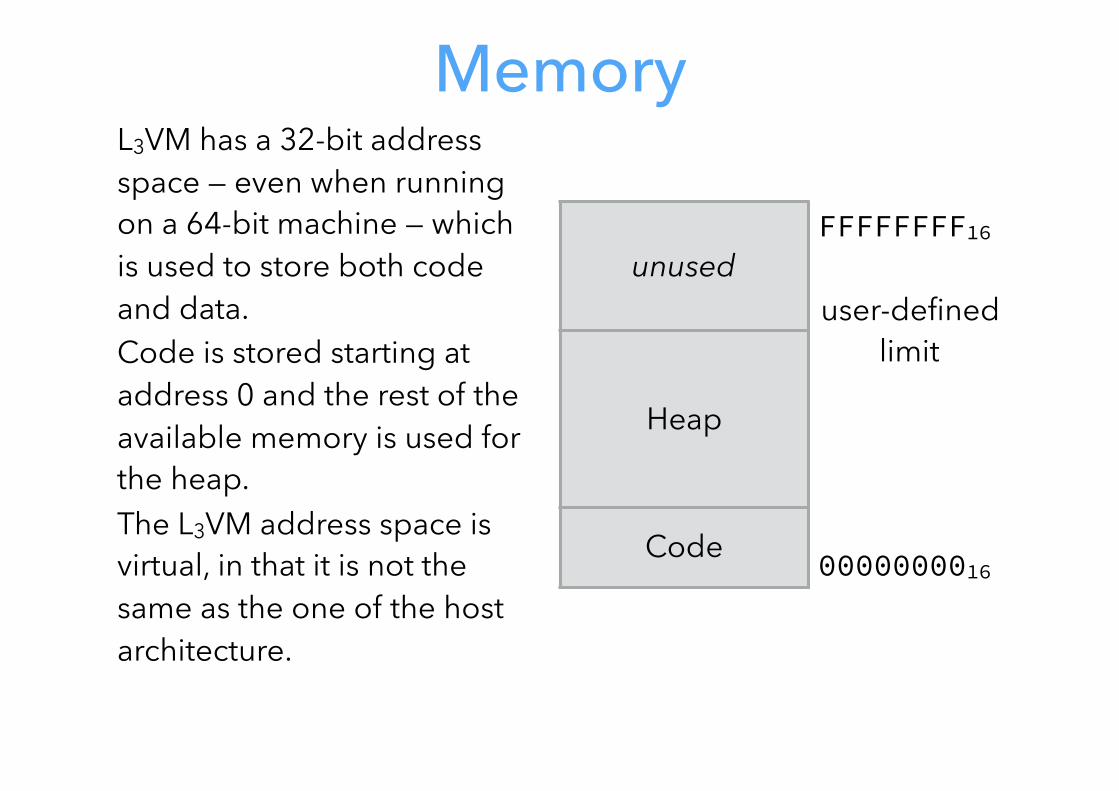
MemoryL3VM has a 32-bit address space — even when running on a 64-bit machine — which is used to store both code and data. Code is stored starting at address 0 and the rest of the available memory is used for the heap. The L3VM address space is virtual, in that it is not the same as the one of the host architecture.
0000000016
FFFFFFFF16unused
Heap
Code
user-defined limit
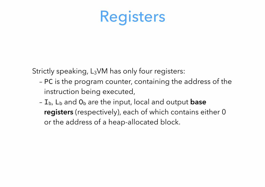
Registers
Strictly speaking, L3VM has only four registers: – PC is the program counter, containing the address of the
instruction being executed, – Ib, Lb and Ob are the input, local and output base
registers (respectively), each of which contains either 0 or the address of a heap-allocated block.
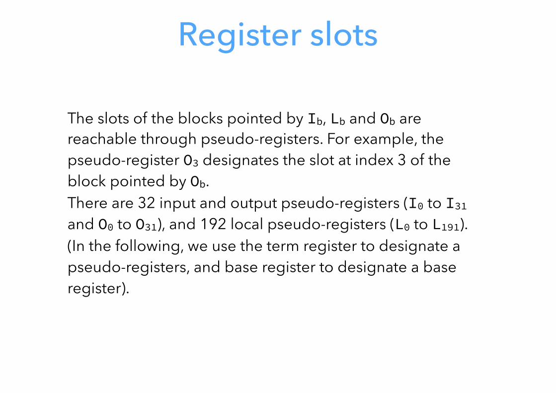
Register slots
The slots of the blocks pointed by Ib, Lb and Ob are reachable through pseudo-registers. For example, the pseudo-register O3 designates the slot at index 3 of the block pointed by Ob. There are 32 input and output pseudo-registers (I0 to I31 and O0 to O31), and 192 local pseudo-registers (L0 to L191). (In the following, we use the term register to designate a pseudo-registers, and base register to designate a base register).
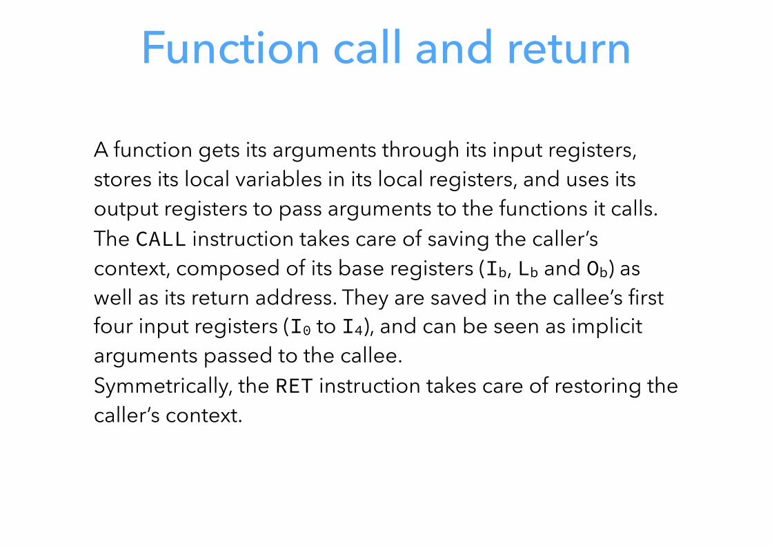
Function call and return
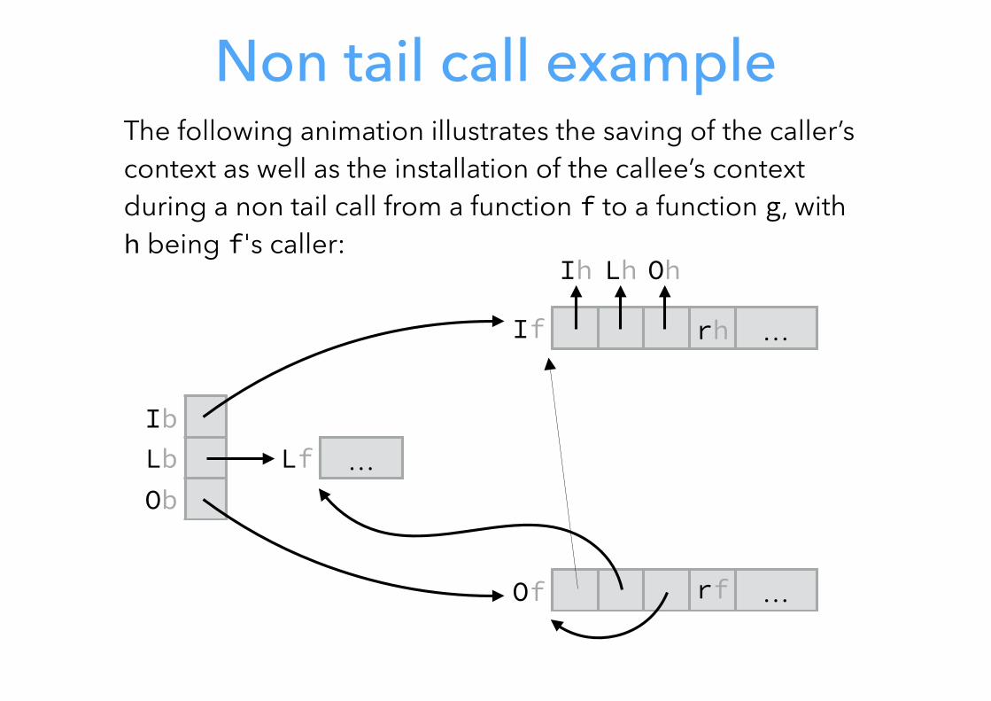
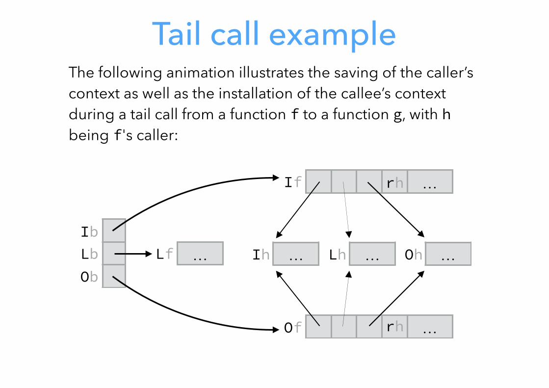
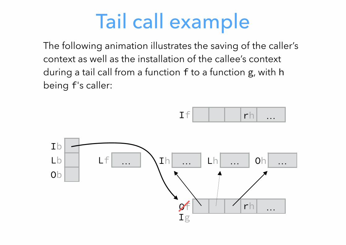
A function gets its arguments through its input registers, stores its local variables in its local registers, and uses its output registers to pass arguments to the functions it calls. The CALL instruction takes care of saving the caller’s context, composed of its base registers (Ib, Lb and Ob) as well as its return address. They are saved in the callee’s first four input registers (I0 to I4), and can be seen as implicit arguments passed to the callee. Symmetrically, the RET instruction takes care of restoring the caller’s context.
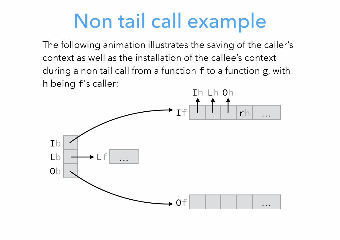
Non tail call exampleThe following animation illustrates the saving of the caller’s context as well as the installation of the callee’s context during a non tail call from a function f to a function g, with h being f's caller:
IbLb Ob
If rh …
Of …
Lf …
Ih Lh Oh
Non tail call exampleThe following animation illustrates the saving of the caller’s context as well as the installation of the callee’s context during a non tail call from a function f to a function g, with h being f's caller:
IbLb Ob
If rh …
Of …
Lf …
rf
Ih Lh Oh
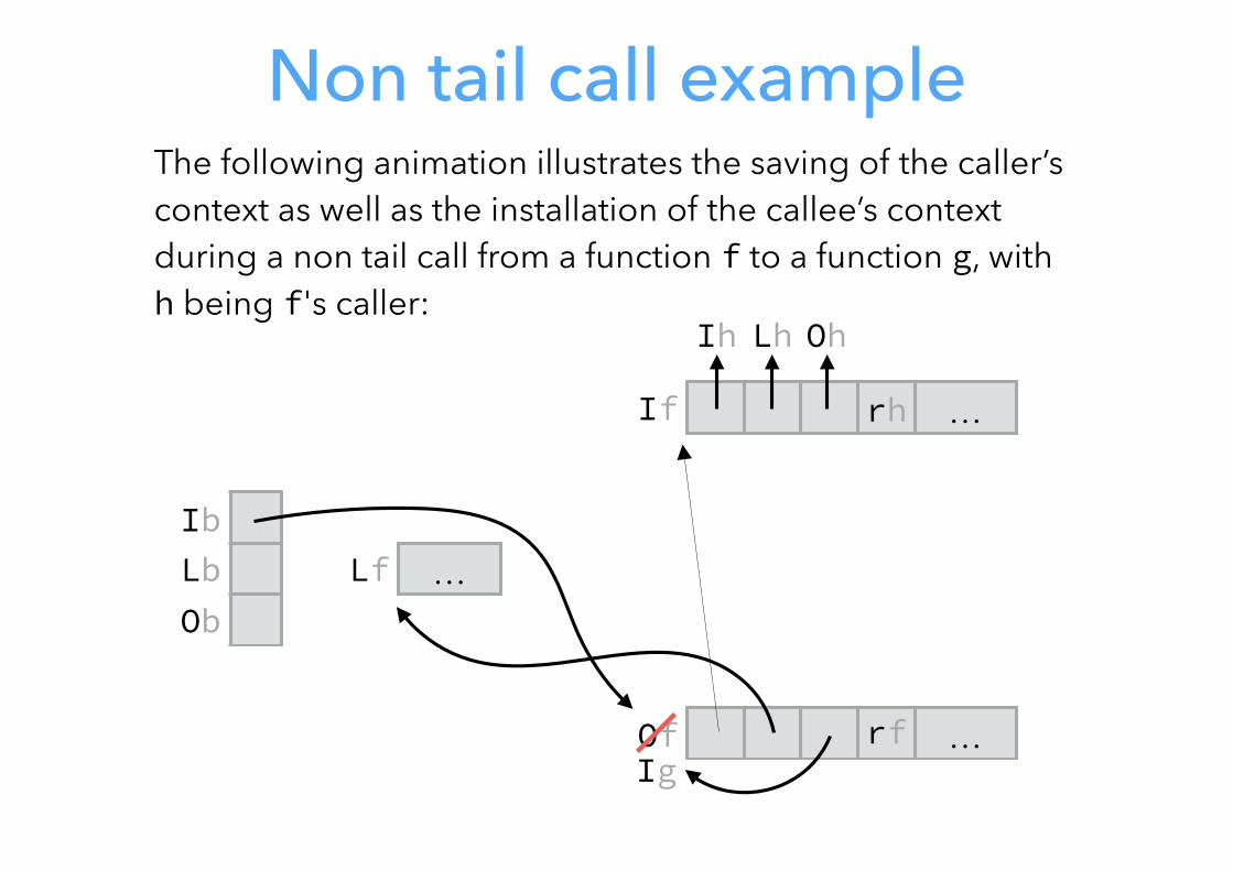
Non tail call exampleThe following animation illustrates the saving of the caller’s context as well as the installation of the callee’s context during a non tail call from a function f to a function g, with h being f's caller:
IbLb Ob
If rh …
Of …
Lf …
rfIg
Ih Lh Oh
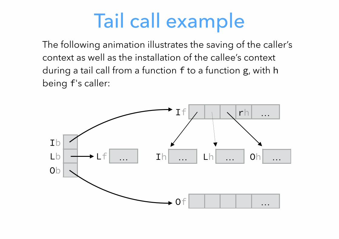
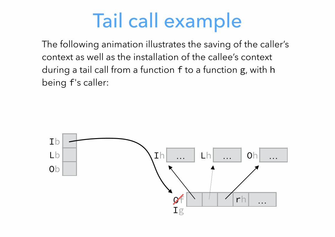
Tail call exampleThe following animation illustrates the saving of the caller’s context as well as the installation of the callee’s context during a tail call from a function f to a function g, with h being f's caller:
IbLb Ob
If rh …
Of …
Lf … Ih … Lh … Oh …
Tail call exampleThe following animation illustrates the saving of the caller’s context as well as the installation of the callee’s context during a tail call from a function f to a function g, with h being f's caller:
IbLb Ob
If rh …
Of …
Lf … Ih … Lh … Oh …
rh
Tail call exampleThe following animation illustrates the saving of the caller’s context as well as the installation of the callee’s context during a tail call from a function f to a function g, with h being f's caller:
IbLb Ob
If rh …
Of …
Lf … Ih … Lh … Oh …
rhIg
Tail call exampleThe following animation illustrates the saving of the caller’s context as well as the installation of the callee’s context during a tail call from a function f to a function g, with h being f's caller:
IbLb Ob
Of …
Ih … Lh … Oh …
rhIg
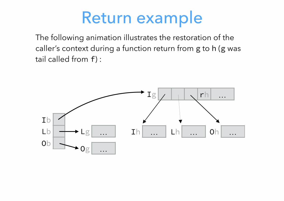
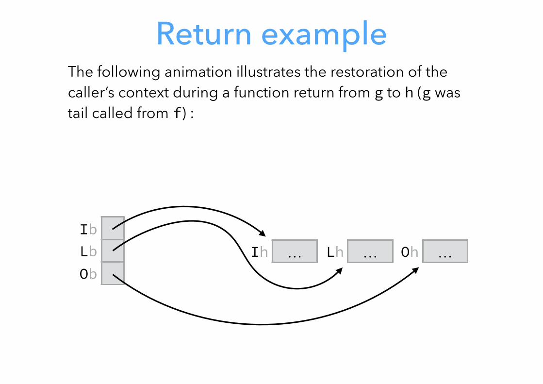
Return exampleThe following animation illustrates the restoration of the caller’s context during a function return from g to h (g was tail called from f) :
IbLb Ob
Ig rh …
Lg … Ih … Lh … Oh …
Og …

Return exampleThe following animation illustrates the restoration of the caller’s context during a function return from g to h (g was tail called from f) :
IbLb Ob
Ig rh …
Lg … Ih … Lh … Oh …
Og …
Return exampleThe following animation illustrates the restoration of the caller’s context during a function return from g to h (g was tail called from f) :
IbLb Ob
Ih … Lh … Oh …
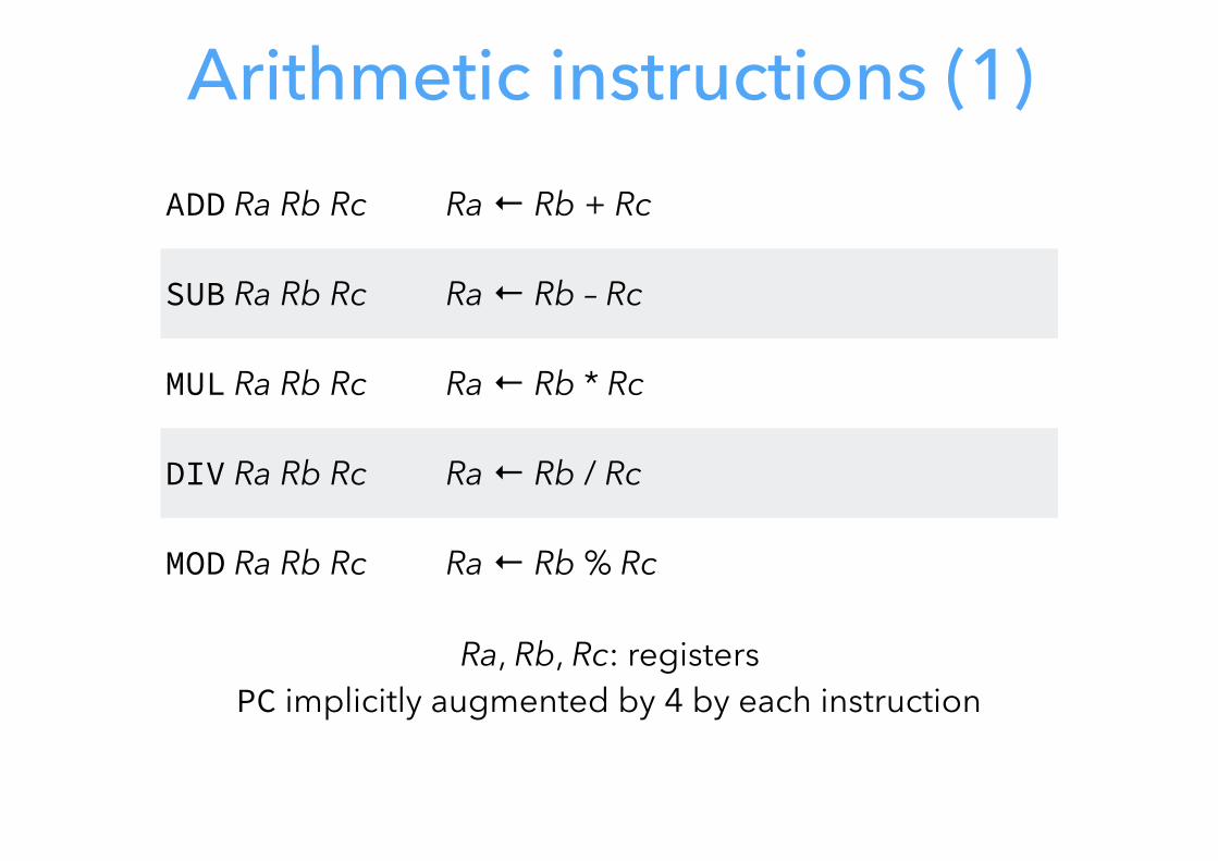
Arithmetic instructions (1)ADD Ra Rb Rc Ra ← Rb + Rc
SUB Ra Rb Rc Ra ← Rb – Rc
MUL Ra Rb Rc Ra ← Rb * Rc
DIV Ra Rb Rc Ra ← Rb / Rc
MOD Ra Rb Rc Ra ← Rb % Rc
Ra, Rb, Rc: registers PC implicitly augmented by 4 by each instruction
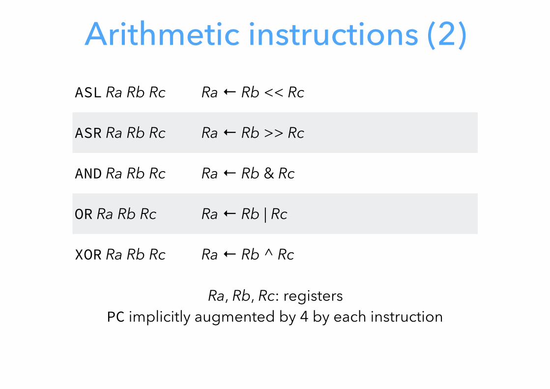
Arithmetic instructions (2)ASL Ra Rb Rc Ra ← Rb << Rc
ASR Ra Rb Rc Ra ← Rb >> Rc
AND Ra Rb Rc Ra ← Rb & Rc
OR Ra Rb Rc Ra ← Rb | Rc
XOR Ra Rb Rc Ra ← Rb ^ Rc
Ra, Rb, Rc: registers PC implicitly augmented by 4 by each instruction
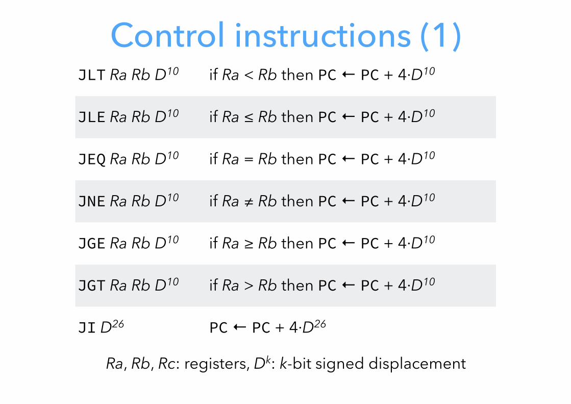
Control instructions (1)JLT Ra Rb D10 if Ra < Rb then PC ← PC + 4·D10
JLE Ra Rb D10 if Ra ≤ Rb then PC ← PC + 4·D10
JEQ Ra Rb D10 if Ra = Rb then PC ← PC + 4·D10
JNE Ra Rb D10 if Ra ≠ Rb then PC ← PC + 4·D10
JGE Ra Rb D10 if Ra ≥ Rb then PC ← PC + 4·D10
JGT Ra Rb D10 if Ra > Rb then PC ← PC + 4·D10
JI D26 PC ← PC + 4·D26
Ra, Rb, Rc: registers, Dk: k-bit signed displacement
Control instructions (2)
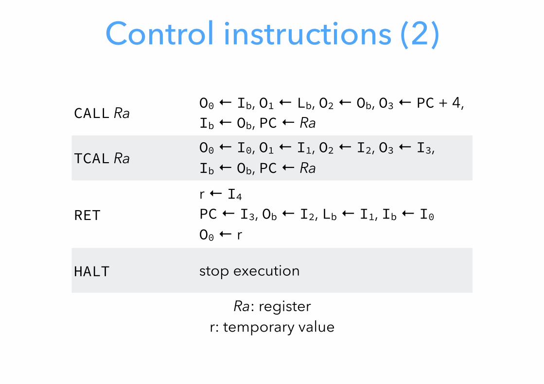
CALL Ra O0 ← Ib, O1 ← Lb, O2 ← Ob, O3 ← PC + 4,Ib ← Ob, PC ← Ra
TCAL RaO0 ← I0, O1 ← I1, O2 ← I2, O3 ← I3,Ib ← Ob, PC ← Ra
RETr ← I4PC ← I3, Ob ← I2, Lb ← I1, Ib ← I0O0 ← r
HALT stop execution
Ra: register r: temporary value
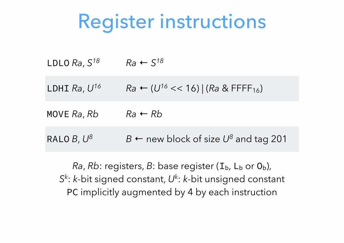
Register instructions
LDLO Ra, S18 Ra ← S18
LDHI Ra, U16 Ra ← (U16 << 16) | (Ra & FFFF16)
MOVE Ra, Rb Ra ← Rb
RALO B, U8 B ← new block of size U8 and tag 201
Ra, Rb: registers, B: base register (Ib, Lb or Ob),Sk: k-bit signed constant, Uk: k-bit unsigned constant PC implicitly augmented by 4 by each instruction
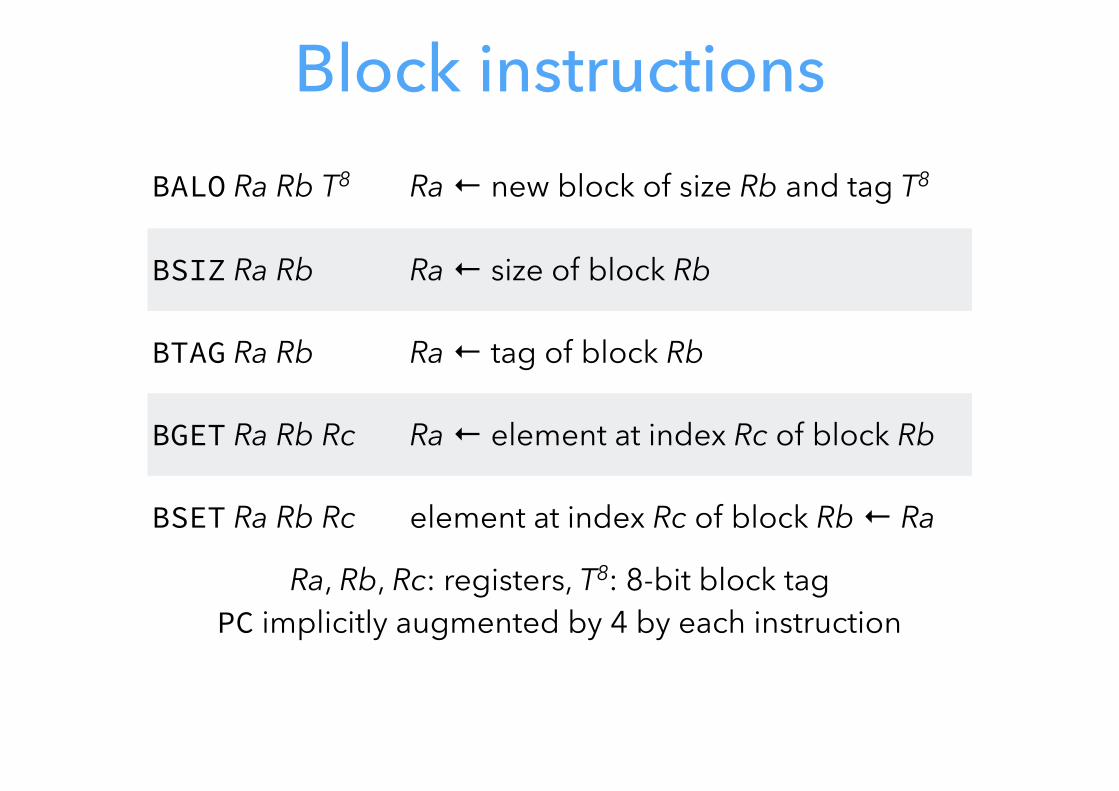
Block instructionsBALO Ra Rb T8 Ra ← new block of size Rb and tag T8
BSIZ Ra Rb Ra ← size of block Rb
BTAG Ra Rb Ra ← tag of block Rb
BGET Ra Rb Rc Ra ← element at index Rc of block Rb
BSET Ra Rb Rc element at index Rc of block Rb ← Ra
Ra, Rb, Rc: registers, T8: 8-bit block tag PC implicitly augmented by 4 by each instruction
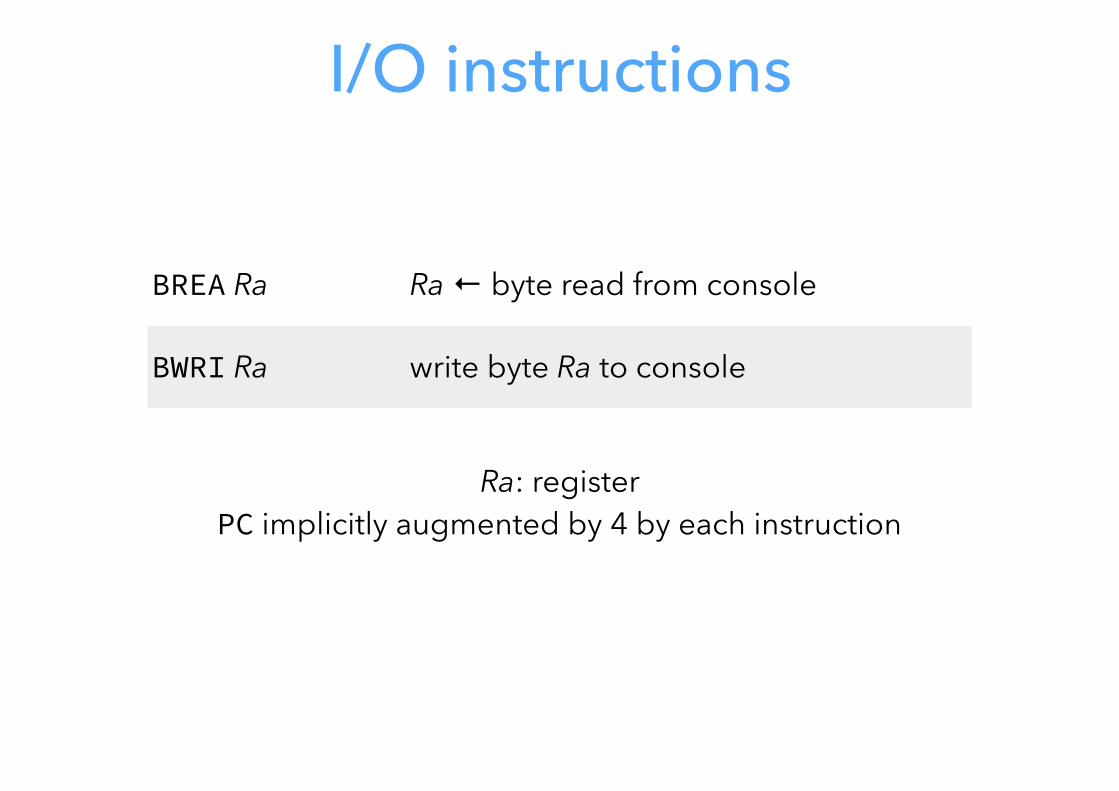
I/O instructions
BREA Ra Ra ← byte read from console
BWRI Ra write byte Ra to console
Ra: register PC implicitly augmented by 4 by each instruction
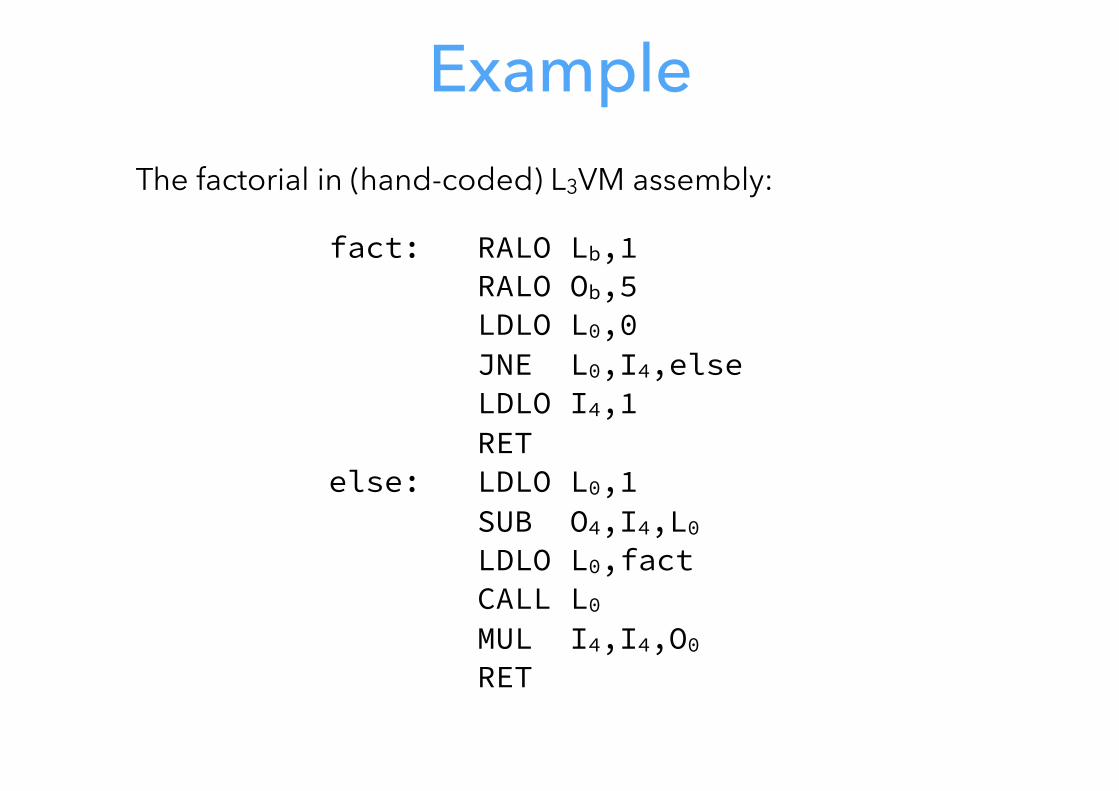
ExampleThe factorial in (hand-coded) L3VM assembly:
fact: RALO Lb,1 RALO Ob,5 LDLO L0,0 JNE L0,I4,else LDLO I4,1 RETelse: LDLO L0,1 SUB O4,I4,L0 LDLO L0,fact CALL L0 MUL I4,I4,O0 RET