interpretationoffalling-headtestsinpresenceof...

International Scholarly Research NetworkISRN Civil EngineeringVolume 2012, Article ID 871467, 10 pagesdoi:10.5402/2012/871467

Research Article

Interpretation of Falling-Head Tests in Presence ofRandom Measurement Error

Paul Chiasson

Department of Civil Engineering, Faculte d’Ingenierie, Univeriste de Moncton, Moncton, NB, Canada E1A 3E9

Correspondence should be addressed to Paul Chiasson, [email protected]

Received 9 February 2012; Accepted 28 February 2012

Academic Editors: H.-L. Luo and S. Pantazopoulou

Copyright © 2012 Paul Chiasson. This is an open access article distributed under the Creative Commons Attribution License,which permits unrestricted use, distribution, and reproduction in any medium, provided the original work is properly cited.

Field data are tainted by random and several types of systematic errors. The paper presents a review of interpretation methodsfor falling-head tests. The statistical robustness of each method is then evaluated through the use of synthetic data tainted byrandom error. Six synthetic datasets are used for this evaluation. Each dataset has an average relative error for water elevation Z,respectively, of 0.04%, 0.11%, 0.22%, 0.34%, 0.45%, and 0.90% (absolute errors on elevation are, respectively, 0.10, 0.25, 0.50, 1.0,and 2.0 mm for a range of water elevation change of 150 mm during test). Each synthetic dataset is composed of 40 synthetic tests(each test consisting of 18 data couples of synthetic falling-head measurements). Results show that the Z-t method is the mostaccurate and precise, followed by the Hvorslev method when a correction is applied and the velocity method when appropriatelyinterpreted. Advice on how to interpret falling-head tests tainted by random error concludes the study.

1. Introduction

A number of methods exist to measure saturated hydraulicconductivity of soils. The constant head test [1, 2] is one ofthese methods. In a laboratory setting, water inlet and outletneed to be maintained at constant elevations. Measurementsof water flow rate in function of hydraulic gradient (headloss per flow path distance) allow the computation of thehydraulic conductivity of the soil using the following equa-tion:

k = − QL(h2 − h1)A

, (1)

where Q is the flow rate, L is the distance separating the twopiezometer measuring tips, hj are measured heads at measur-ing tips 1 and 2, and A is cross-section of the permeameter.ASTM [1, 2] is a good source for permeameter designand testing methodologies. When performing hydraulic con-ductivity tests in the laboratory, Chapuis et al. [3] stressthe importance of good saturation. They describe a testingprotocol to reach and measure saturation levels of testedsamples.

Constant head tests can also be performed in the field.CAN/BNQ [4, 5] describe methods where water is injected in

a cased borehole at a constant head in an aquifer or aquitardunder steady state conditions [6]. Hydraulic conductivity canthen be computed by using

k = − Q

C(h2 − h1), (2)

where C is a shape factor that is, for example, 2.75 times theinner diameter D for an end of casing test, h1 is the total headof water in the cased borehole, and h2 is the total head of thefree surface (or piezometric level) of the tested soil layer. Thismethod is based on the hypothesis that the injected volumeof water will have negligible influence on the piezometriclevel (PL) of the soil surrounding the injection zone.

When testing low hydraulic conductivity soils, the maindrawbacks of constant head tests are that they are extremelylengthy in time, and, in the case of field tests, the PL of thesoil layer may be unknown or difficult to measure. Falling-head tests are effective answers to both these drawbacks. Theycan be completed in a short-time span and Chapuis et al. [7]demonstrated that their interpretation does not necessitatethe PL of the surrounding soil layer.

Field (and laboratory) data are generally tainted withmeasurement errors. These are of two types, systematic andrandom errors. A systematic error is, for example, created to

2 ISRN Civil Engineering

the total head by incorrect calibration of a piezometer. Thistype of error can be constant in time or can follow some sortof time drift. Random errors are characterized by a zero meanand some standard deviation. These errors are the result of anumber of phenomena. Human reading of a standpipe scaleand white noise due to electrical interference in piezoelectrictransducers are examples. Piezoelectric transducers also yieldstep-wise data due to conversion of analog values to digitalcode. Measurements are then higher or lower than truevalues.

This paper will review the theoretical background for theinterpretation of falling-head tests when in presence of ran-dom errors. Five (5) interpretation methods are presented:log (or Hvorslev), traditional interpretation of velocity(or Chapuis), alternate interpretation of velocity, Z-t andoptimised log (or corrected Hvorslev). Each method will beapplied on synthetic datasets. Data within each set includesa random error component of predefined variance. Theobject will be to evaluate how each interpretation methodis sensitive to random measurement error. A comparisonbetween methods and a discussion on the interpretation offalling-head tests will follow.

2. Interpretation of Falling-Head Tests

Data from falling head tests, be they obtained in thelaboratory or in the field, may be interpreted by a number ofmethods. Chapuis [8] indicates that when the deformationsof the soil can be neglected, falling-head tests are governed bythe Laplace equation. Its solutions, the harmonic functions,have several properties. One of them relates flux into the soil(Qsoil) to flow into the pipe (Qinj) through a mass-balanceequation:

Qinj = Qsoil = ckH , (3)

where c is a shape factor that depends on the geometry ofthe injection zone and on the hydraulic boundaries of theproblem, H is the applied hydraulic head difference, and kis the hydraulic conductivity. This equation is the startingpoint of the Hvorslev, velocity (Chapuis), and Z-t methods.Another equation is the starting point of another method forcases where the soil deformation is assumed to be elastic andnot negligible [9]. However, this method contains physicaland mathematical confusions according to the mathematical,physical, and numerical proofs by Chapuis [8] and theexperimental proofs of Chapuis and Chenaf [10]. Accordingto the equations of Chapuis [8], the effect of soil deformationcan be neglected when the soil is an aquifer or an overconsol-idated aquitard. It is no longer negligible for compressibleaquitards when they are tested using either a falling-headtest with a very small injection pipe or a pulse test betweenpackers. Chapuis and Cazaux [11] gave suggestions on howto correctly handle the instantaneous (elastic) and delayeddeformations in such cases. In a falling-head test, Qinj is theflow through the inflow pipe (often a standpipe connected tothe borehole casing) of internal cross-section Sinj:

Qinj = −SinjdH

dt, (4)

where t is time. Equations (3) and (4) yield

dH

dt= − c

SinjkH. (5)

Rearranging gives

dH

H= − c

Sinjkdt. (6)

Integrating leads to the solution proposed by Hvorslev [12]:

ln

(Hj

Hj+1

)= −kC

(t j − t j+1

), (7)

where Hj is the instantaneous head loss at time t j obtainedfrom the difference between the total heads in the inletstandpipe and PL at the boundary of the surroundingsoil, and C = c/Sinj is a shape factor that depends on theinlet/outlet geometry. Hvorslev [12] compiled shape factorsfor a number of inlet/outlet geometries. For field conditionsillustrated in Figure 1, shape factor C is

C = 11Dπd2

, (8)

where D and d are, respectively, the internal diameters ofthe casing and of the standpipe. For laboratory falling-headtests, C is given by

C = A

aL, (9)

where A is the area of the permeameter cross-section, “a”is the cross-section of the inlet standpipe, and L is the flowdistance through the soil sample. In the laboratory, theoutlet is a constant head basin controlled by an overflowweir. In the field, the outlet head is set by the geometry andthe boundary conditions of the surrounding soil, that is, thePL. In the laboratory, it is relatively easy to accurately andprecisely measure the outlet piezometric head. In the field,an accurate measure of the PL of the surrounding soil is notnecessarily trivial. An error in the PL value will introduce abias or systematic error of constant value in head differenceHj of (7). Chapuis [13] showed that this systematic errorwill produce a curved ln(H) versus time plot. Since thehydraulic conductivity k is the slope of this plot, a curvedplot wrongly suggests that k changes with time. A concavedownward curve suggests that k increases during theduration of the test. If the test is repeated assuming the samesystematic error in the PL of the surrounding soil, the samecurved plot will be observed. Chiasson [14] mathematicallydemonstrated that when the systematic error in the PL of thesurrounding soil is not zero (i.e., H0 /= 0), the relationshipbetween hydraulic conductivity and the slope of the plot asexpressed by (7) is no longer valid. Thus the direct use of (7)as proposed by Hvorslev without questioning the PL value isfaulty practice [13]. Chiasson [15], furthermore, concludesthat Hvorslev’s equation is incomplete and proposes acorrection to this method and an interpretation through logoptimization. This is described later in the paper.

ISRN Civil Engineering 3

D

d

Z(t)

H(t)

H0

Figure 1: Setup for a falling-head test in an unconfined aquifer (oraquitard).

2.1. Traditional Interpretation of the Velocity Plot. The veloc-ity method proposed by Chapuis et al. [7] is one wherethe unknown PL of the soil is not needed for hydraulicconductivity determination. Therefore, a systematic error inthe assumed PL has no consequence in computations ([16]as quoted by [13]). For this method, the following definitionis first introduced:

H(t) = Z(t) + H0, (10)

where H0 is the vertical distance between Z(t), the elevationabove ground of the inlet falling water level within thestandpipe, and the PL of the surrounding soil (Figure 1). IfZ(t) is erroneously assumed as the total head loss betweeninlet and the PL of the soil, H0 can be seen as the systematicerror, or bias. Rearranging (5) using (10) then gives

Z = − 1Ck

dZ

dt−H0 = mv

dZ

dt−H0. (11)

By plotting y = Z as a function of x = v = dZ/dt, astraight line should be obtained with slope mv = −1/Ck andintercept H0. Thus, the slope of this plot is related to k by

k = − 1mvC

. (12)

Choosing Y = Z and X = v defines the traditional velocityplot. Modern spreadsheets permit to easily compute the slopemv using the least squares method, a best linear unbiasedestimator (BLUE).

The velocity plot has many advantages. A part fromestimating hydraulic conductivity, it can be used to graphi-cally obtain the systematic error (if any) of the assumed PL,identify hydraulic fracturing during the test ([7, 17, 18] inpiezometers) or consolidation at the beginning of the test ofthe soil surrounding the tip of the borehole [8, 19], and evenidentify leakage in buried pipes [20].

2.2. Alternate Interpretation of the Velocity Plot. Interpre-tation of the velocity method using the method of leastsquares should yield the best unbiased linear fit. Chiasson[15] underlined that statistical estimation by least squaresis theoretically based on one dependant variable being afunction of another that is independent. The independentvariable is a controlled variable; that is, it is the user thatdecides at which value a measurement of the dependantvariable will be made. Thus, by definition, the independentvariable has no measurement error.

In the traditional interpretation of the velocity method,velocity v during a time increment Δt is considered as theindependent variable and the average elevation Zm = (Zj +Zj+1)/2 during the same time increment is the dependentvariable. When data has low scatter in Z (or t), this haslittle effect on the result. When data has some scatter in Z(or t), Chiasson [14, 15] shows that interpretation problemsarise! The act of choosing v as the controlled variable whenit has high statistical scatter clearly departs from least squareestimation theory.

Between variables v and Zm, Zm displays the leastmeasurement error. One could thus choose to consider Zas the control variable and time t could be measured at acertain value of Z. With Zm as the control variable, velocityv = ΔZ/Δt is the dependant variable. This makes more sensesince by definition velocity v is a function of elevation Z andtime t, that is, it is dependent on Z and t. Rearranging (11)to isolate v on the left hand side gives

v = dZ

dt= −CkZ − CkHo = mZZ + bZ. (13)

From (13), the hydraulic conductivity k and the bias H0 are:

k = −mZ

C, (14)

H0 = bZmz

. (15)

2.3. Z-t Method. A third method proposed by Chiasson [14]plots raw elevation data Z as a function of time t. Thesolution for (6) using (10) is as follows (see Chiasson fordemonstration):

Z = Hie−at −H0, (16)

where Hi is the head difference at initial time t j = t0 = 0 and“a” is an exponent parameter where

k = a

C. (17)

Let Zj be the measurement of Z at time t j , for j = {0, . . . n},and let Z∗(t j) be the estimated water level in the standpipeat time t j , using estimated parameters Hi

∗, a∗, and H∗0 . The

best unbiased estimator will then be obtained by numericallyminimising the following equation:

MIN

⎛⎝ n∑

j=0

[Zj − Z∗

(t j)]2

⎞⎠ (18)


while being subjected to the unbiased condition:

n∑j=0

[Zj − Z∗

(t j)]= 0. (19)

2.4. Correction to the Hvorslev Method or Optimised Log [Z +H0] Method. In the traditional interpretation of Hvorslev’smethod, log(Hj/Hi) is plotted as a function of time t. Indoing this, Hvorslev made two implicit suppositions that H0

is known a priori and that the initial reading for Hi at timet0 = 0 has no measurement error. Clearly, this can neverbe perfectly the case. These two assumptions will only beapproximately true, the extent of the approximation beinga function of error. Chapuis [13] and Chiasson [14] showhow making these implicit suppositions will adversely affectthe interpretation of the test and the value of the hydraulicconductivity k. The interpretation process could use thevelocity method to determine H0 and interpret the falling-head test by rearranging (7) using (10) to obtain

ln(Zj + H0

)= −kCtj + ln(Z0 + H0) (20)

and to plot y = ln(Zj + H0) in function of x = t. Unfor-tunately, this approach is incomplete since it implicitly makesthe supposition that the initial reading at time t0 = 0 hasno measurement error. Since the error on the first readingZ(t = 0) = Z0 is usually small, the initial solution Hi

of (16) is approximately equal to Z0 + H0. (where Z0 ismeasured and H0 is estimated by the velocity method) Thus,the hydraulic conductivity computed this way will generallynot be adversely affected. This interpretation is found toyield hydraulic conductivity values that are always close tobeing equal to the value obtained by the velocity method.Since two methods give the same result, one could concludethat this confirms the validity of the hydraulic conductivityvalue. Chiasson [14] shows that if H0 and Hi are obtainedby another interpretation method, that is, the Z-t method,interpretation of a falling-head test using (20) will give valuesequal to those obtained by the Z-t method! This bringsChiasson to conclude that (20) (Hvorslev’s method) with H0

estimated from another method (velocity or Z-t) cannot beused to confirm the validity of the k value obtained by thesame other method (velocity or Z-t), since the value of k thatis obtained is dependant of the method used to estimate H0.

A remedy to this is to correct Hvorslev’s method byestimating H0, Hi, and k by a least squares optimisation tech-nique similar to the one used in the Z-t method. Rewriting(20) with Hi = Z0 + H0, mln = −kC, and bln = ln(Hi) gives

ln(Zj + H0

)= mlnt j + bln. (21)

Let then y∗ = ln(Z∗(t j) + H0) be the estimated naturallogarithm of the total head in the standpipe at time t j , withestimated parameters b∗ln = ln(H∗

i ), m∗ln = −k∗C, and

H∗o . The best unbiased estimator will then be obtained by

numerically minimising the following equation:

MIN

⎛⎝ n∑

j=0

[yj − y∗

(t j)]2

⎞⎠ (22)

while being subjected to the unbiased condition

n∑j=0

[yj − y∗

(t j)]= 0. (23)

This variant of Hvorslev’s log method independentlyestimates all unknown parameters. Theoretically, it can beused to separately evaluate k and confirm values estimatedby both velocity and Z-t methods.

3. Performance of Interpretation Methods orTheir Statistical Robustness

The synthetic tests presented here correspond to conditionsencountered in overconsolidated aquitards such as com-pacted clay liners (CCLs) used in solid waste cells. Thesehave hydraulic conductivities in the order of 1 × 10−6 mm/swith a typical thickness of one metre. CCL are also veryrigid in nature due to the applied high energy compaction.Both high rigidity and limited thickness minimize effects onthe local PL of immediate and delayed aquitard deformation[21]. Furthermore, the velocity plot will yield a straight linewhen pore water volume change is negligible [8] and straightvelocity plots are observed in tests performed on CCLs (see,e.g., [14]).

The solution for differential equation (6) expressed by(16) with Hi = 701 mm, H0 = 400 mm, and k = 5×10−7 mm/sand a test setup giving a shape factor C = 235.3 mm−1 wasused to generate synthetic data as follows:

Z =[

(701 mm)e−1.176×10−4t − 400 mm]

+ ε, (24)

where ε is a normal law distributed random fluctuationwith zero mean and standard deviation σ = ΔZ/1.96. Therandom fluctuation component corresponds to a syntheticrandom measurement error. By definition, ΔZ is the absoluteerror of the synthetic dataset composed of measurementsZ. Six synthetic datasets of increasing absolute error on Zwere generated this way. Absolute errors for each syntheticdataset will be in increasing order ΔZ =: ±0.10 mm,±0.25 mm, ±0.50 mm, ±0.75 mm, ±1.0 mm and ±2.0 mm.Error relative to the range of elevation change (ΔZ/[Zmax −Zmin]) thus spans from 0.07% to 1.3%. Each absolute errordataset is composed of 40 synthetic tests with each testcomposed of 18 synthetic measurements spanning from t =0 to 2040 seconds. During each synthetic tests, elevation inthe standpipe drops by 150 mm. Note that in the experienceof the author, absolute errors of ±2.0 mm in datasetsobtained from cased borehole tests in compacted clay linersare not uncommon (see, e.g., [14]).

Each method reviewed earlier is applied to these sixsynthetic datasets to investigate their sensitivity to datatainted by random measurement error.

3.1. Traditional Velocity Plot. As underlined earlier, whenmeasurement errors on Z are small, interpretation by leastsquares of the traditional velocity plot will yield good results.An illustration of this statement is given in Figure 2. In this


Zm = −8422.3v − 394.5

R2 = 0.9795

0

100

200

300

400

−0.1 −0.05

Ave

rage

ele

vati

onZm

(mm

)

Velocity (mm/s)

Test dataLeast squares

Figure 2: Velocity plot of synthetic test data with very low meas-urement error (ΔZ = ±0.10 mm).

plot, the measurement error on Z is only of ±0.10 mm.Least squares yield mv = −8422.3 sec−1 (Figure 2), C =235.3 mm−1, (12) gives k = 5.05 × 10−7 mm/s and H0 =394.5 mm. Both hydraulic conductivity k and bias H0 are byall practical means equal to the no-error-imposed solution ofH0 = 400 mm and k = 5 × 10−7 mm/s. This gives a relativeerror of only 0.92% for k and 1.4% for H0.

When relative measurement error on Z is significant(in the order of ΔZ/[Zmax − Zmin] = 0.7%), the velocityplot displays considerable scatter (Figure 3). Such a plot willsuggest that data from the test are of questionable quality.With the same shape factor and (12), one finds by leastsquares mv = −2643.6 sec−1 giving a hydraulic conductivityk = 1.61 × 10−6 mm/s and H0 = −28.8 mm. This is a222% relative error on k and −107% relative error on H0.Hence, relatively small measurement errors in elevation Zyield appreciable estimation errors for k and Ho.

Chiasson [15] observes that interpretation by leastsquares of the traditional velocity plot systematically giveshigher k values than the methods earlier presented. The sixsynthetic datasets, generated by (24) with ΔZ: ±0.10 mm,±0.25 mm, ±0.50 mm, ±0.75 mm, ±1.0 mm, and ±2.0 mm,confirm this systematic bias (Figure 4). Also, as absolutemeasurement error increases on Z, so does the average andstatistical scatter of the hydraulic conductivity obtained bythe velocity method. Thus, this method of interpretation, fordata subjected to measurement error, produces a systematicbias in the interpreted k value.

There is a clear trend between measurement error on Zand the hydraulic conductivity obtained from least squaresof the traditional velocity plot (average trend in Figure 4).Furthermore, a good correlation is observed between therelative error (Δk/k) on the value of k obtained by thevelocity plot and the coefficient of determination of the same

0

100

200

300

400

−0.1 −0.05

Ave

rage

ele

vati

onZm

(mm

)

Velocity (mm/s)


Z = −2643.6v + 28.786

R2 = 0.2749

Figure 3: Velocity plot of synthetic test data affected by measure-ment error (ΔZ = ±1.0 mm).

1E − 07

1E − 06

1E − 05

0 1 2

Hyd

rau

lic c

ondu

ctiv

ityk

(mm

/s)

Average trend

Solution (no error)

Maximum

Median

Minimum

75

25th percentile

Absolute error ΔZ (mm)

th percentile

Figure 4: Scatter of hydraulic conductivity values as interpretedby velocity method in function of absolute error ΔZ of syntheticdatasets.

plot (Figure 5). This further demonstrates that interpretationby least squares of the traditional velocity plot is notstatistically robust. Based on this work and on Chiasson [14],least squares of the traditional velocity plot must not be usedin a straightforward manner on raw data when scatter isobserved. That is when R2 is less than 0.92. Coefficients ofdetermination higher than this threshold will yield relativeerrors on k below 10% (Figure 5).


0

50

100

150

200

0 0. 5 1

Rel

ativ

e er

rorΔ

k/k

(%

)

R2

Δk/k = 3.73(R2)2

−8.04(R2) + 4.3

Figure 5: Relative error on hydraulic conductivity k in functionof coefficient of determination R2 obtained from velocity methodplots.

The above analysis shows that increasing statistical scatterin the velocity plot decreases the slope of the least squares line(and increases the interpreted k value). The value of interceptH0 will as a consequence decrease in a concurrent fashion.This result for the estimated slope value is in accordancewith a relationship between the true slope and the slopeestimated by least squares as presented by Snedecor and([22] unfortunately, the coefficient of the relationship is oftendifficult to determine). Thus, least squares of the traditionalvelocity plot must not be used to extract the correct (or true)piezometric level at the injection point when the coefficientof determination R2 is below 0.92.

Velocity plot scatter can be reduced in cases where thenumber of data couples is sufficiently high. In such cases,Chapuis [21] proposes a five-step interpretation procedureto reach this goal. When datasets are too small, least squaresof the traditional velocity plot must not be used to extractk and H0. Nevertheless, It remains warranted to prepare avelocity plot to confirm, as earlier underlined, that it is linearand that no other phenomena intervenes during the test.

3.2. Alternate Interpretation of the Velocity Plot. An appro-priate interpretation of the velocity method should be onethat uses as the X variable the measurement with minimalerror, reserving the role of Y to the other. The samedata that was plotted in Figure 3 is used to illustrate thisalternative interpretation. The permuted plot, where velocityv is in function of average elevation of falling-head Zm, doesnot yield a better correlation coefficient, since it measuresscatter and this is unchanged (Figure 6). The hydraulicconductivity computed from this plot is on the other handsignificantly different (it is lower). Using (14), the same shapefactor C and the least square slope mZ (Figure 6) yields

v = −0.000104 Zm − 0.050344

R2 = 0.274948

0 100 200 300 400−0.1

−0.05

Average elevation Zm (mm)

Vel

ocit

y (m

m/s

)


Figure 6: Permuted velocity plot for data of Figure 3 (synthetic testdata with ΔZ = ±1.0 mm).

k = 4.42 × 10−7 mm/s and H0 = 484 mm. With thepermuted plot, relative error on k has decreased to −11.6%and to 21.0% for relative error on H0. This is a considerableimprovement in relation to the 222% relative error fork and −107% relative error for H0 that was obtainedearlier with least squares of the traditional velocity plot.Computed hydraulic conductivity values from this “alternateinterpretation” of the velocity method show no correlationwith test data scatter as characterised by the coefficient ofdetermination (Figure 7).

On average, the alternate interpretation of the velocitymethod will yield good hydraulic conductivity values. Onthe other hand, scatter in measurements, although lessproblematic than with the traditional interpretation of thevelocity method, will still yield rather high relative errors(Δk/k) for k (Figure 8). The alternate interpretation can thusbe qualified as being unbiased, that is, on average accuratebut not precise. Results from this study indicate that thealternate interpretation should be used with caution whendata scatter in the velocity plot yields R2 less than 0.87.Otherwise, relative error on the k value may be greater than±10% (Figure 7). The same observations apply for interceptH0 (Figure 9). When R2 is less than 0.87, it is recommendedto follow the five steps interpretation procedure proposed byChapuis [21] but using least squares on X-Y variables of thealternate velocity plot.

3.3. Z-t Method. Chiasson [14] introduced this method afterobserving that scatter in the velocity plot (likewise with thepermuted velocity plot) is inherent to the computation ofthe velocity ([21] gives the equation of the relative error).Chiasson thus proposes to use raw data, that is, [t j , Zj] datacouples, and directly plot them on a Z-t graph. Difference


0 0. 5 1

R2

100

0

−100

Rel

ativ

e er

rorΔ

k/k

(%)

Δk/k = 0.086 R2 − 0.103

R2 = 0.0137

Figure 7: Relative error on hydraulic conductivity k in function ofcoefficient of determination R2 obtained from alternate interpreta-tion of the velocity method.

Maximum

Median

Minimum

1E − 07

1E − 06

1E − 05

0 1 2

Hyd

rau

lic c

ondu

ctiv

ityk

(mm

/s)

Average trend

Solution (no error)


75

25th percentile

th percentile

Figure 8: Scatter of hydraulic conductivity values obtained fromthe alternate interpretation of the velocity method in function ofabsolute error ΔZ of synthetic datasets.

in scatter amplitude is evident when comparing scatter in avelocity plot (or permuted velocity) with scatter in a Z-t plot(compare Figures 3 and 6 with Figure 10).

Applying the Z-t method to the same dataset earlier usedwith traditional and alternate interpretations of the velocitymethod gives k = 4.68 × 10−7 mm/s, H0 = 439.5 mm andHi = 739.9 mm. This corresponds to a relative error for kof −6.4% and of 9.9% for relative error on H0. This is animprovement comparative to earlier presented methods, be itthe traditional or alternate interpretation of the velocity plot.

Maximum

Median

Minimum

0 1 2

Average trend

Solution (no error)

0

200

400

600

800

1000

1200

H0

(mm

)


75

25th percentile

th percentile

Figure 9: Scatter of intercept value (H0) obtained by the alternateinterpretation of the velocity method as a function of absolute errorΔZ of synthetic datasets.

150

200

250

300

350

0 1000 2000 3000

Time (seconds)

Test data

Ele

vati

onZ

(mm

)

Fitted Z∗

Figure 10: Z-t plot for data of Figure 3 (synthetic test data with ΔZ= ±1.0 mm).

The Z-t method is unbiased; that is, there is no significantcorrelation with scatter intensity (Figure 11). It yieldedhigh coefficients of determination for the complete suite ofstudied absolute errors, meaning that (16) well explains therelationship between Z and t.

The Z-t method yields good hydraulic conductivity val-ues and it is less sensitive to data scatter (Figures 11 and 12).


1

100

0

−100

Rel

ativ

e er

rorΔ

k/k

(%)

0.999 0.9995

R2

Δk/k = 37.01 R2 − 37.01

R2 = 0.0058

Figure 11: Relative error of hydraulic conductivity k in function ofcoefficient of determination R2 obtained from Z-t method.

1E − 07

1E − 06

1E − 05

0 1 2

Hyd

rau

lic c

ondu

ctiv

ityk

(mm

/s)

Average trend

Solution (no error)

Maximum

Median

Minimum


75

25th percentile

th percentile

Figure 12: Scatter of hydraulic conductivity values as interpreted byZ-t method in function of absolute error ΔZ of synthetic elevations.

It is thus an accurate interpretation method. It is also aprecise method since relative error on k is of only 3.6%when synthetic data has ΔZ = 0.25 mm and increasesby approximately the same increment for each 0.25 mmincrement to ΔZ. Results from this study indicate that the Z-t method can be used even when absolute errors on Z are ofthe order of 2.0 mm (ΔZ/Z = 1.3%) for which relative erroron k will be of 28.4%.

The same behavior is also observed for intercept valuesH0, that is, no systematic error (accurate value). Relativeerrors ΔH0/H0 are smaller than in both earlier discussed

Maximum

Median

Minimum

1E − 07

1E − 06

1E − 05

0 1 2

Hyd

rau

lic c

ondu

ctiv

ityk

(mm

/s)

Average trend

Solution (no error)


75

25th percentile

th percentile

Figure 13: Scatter of hydraulic conductivity values as interpretedby corrected Hvorslev method in function of absolute error ΔZ ofsynthetic elevations.

methods although they are 1.6 times higher than hydraulicconductivity relative errors Δk/k. Thus, the Z-t method givesan accurate value for intercept H0 and gives the highestprecision.

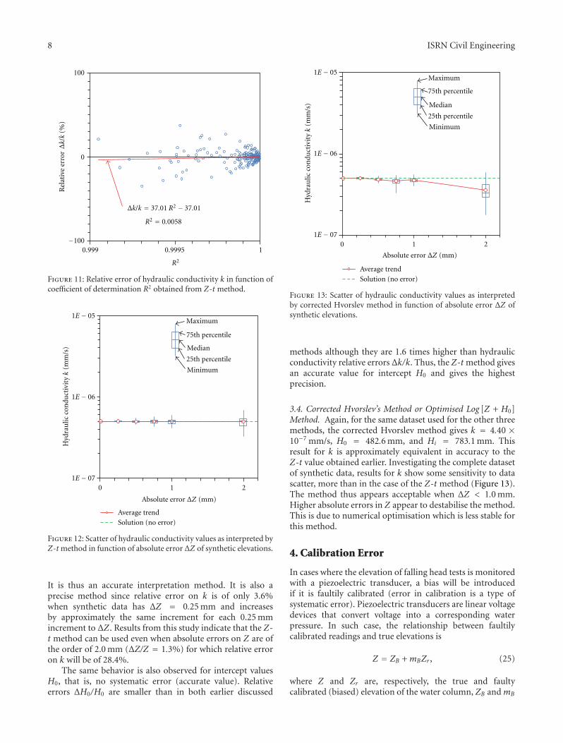
3.4. Corrected Hvorslev’s Method or Optimised Log [Z + H0]Method. Again, for the same dataset used for the other threemethods, the corrected Hvorslev method gives k = 4.40 ×10−7 mm/s, H0 = 482.6 mm, and Hi = 783.1 mm. Thisresult for k is approximately equivalent in accuracy to theZ-t value obtained earlier. Investigating the complete datasetof synthetic data, results for k show some sensitivity to datascatter, more than in the case of the Z-t method (Figure 13).The method thus appears acceptable when ΔZ < 1.0 mm.Higher absolute errors in Z appear to destabilise the method.This is due to numerical optimisation which is less stable forthis method.

4. Calibration Error

In cases where the elevation of falling head tests is monitoredwith a piezoelectric transducer, a bias will be introducedif it is faultily calibrated (error in calibration is a type ofsystematic error). Piezoelectric transducers are linear voltagedevices that convert voltage into a corresponding waterpressure. In such case, the relationship between faultilycalibrated readings and true elevations is

Z = ZB + mBZr , (25)

where Z and Zr are, respectively, the true and faultycalibrated (biased) elevation of the water column, ZB and mB


are constant and scale biases. Using (25), the true velocity (ifcoefficients ZB and mB were known) would be

ΔZ

Δt= mB

(ZR, j+1 − ZR, j

t j+1 − t j

). (26)

This defines the relationship between true velocity (at left)and faultily calibrated velocity (at right):

ΔZ

Δt= mB

ΔZR

Δt. (27)

According to (11), using (25), the relationship between faultyvelocity and faulty elevation of the water column is:

ZR = mvdZR

dt− (H0 + ZB)

mB. (28)

This later equation shows that the plot of faulty elevationin function of faulty velocity has the same slope as oneobtained from true elevation and velocity, that is, (11).Then, according to (11), the faulty plot will give the correcthydraulic conductivity. This is not the case for the interceptvalue as can be viewed by comparing (28) and (11). Since theintercept defines the piezometric level (Figure 1), the plot offaulty calibrated readings will not yield a correct PL.

Since the same equations are used to prepare thealternate velocity plot, the same conclusions will also apply.Developing (15) with (25) will find the same results for theZ-t method and (21) with (25) will yield the same for thecorrected Hvorslev method.

When the PL is of importance, and it is certainly oftenthe case, a verification of calibration needs to be performed.If when performing the falling head test, the elevation of themeasuring tip of the piezoelectric transducer is noted, it isthen possible to back calculate the PL value after calibrationof the transducer in the laboratory. For the case of piezo-electric transducers in open piezometers, a field comparisonbetween transducer readings and direct measurements ofwater elevation will permit to obtain correct calibration.

5. Conclusion

Interpretation methods for falling-head tests were evaluatedfor their sensitivity to measurement error in elevationsmeasurements of the falling water column. Least squares ofthe traditional velocity plot are found to be the less appro-priate approach for interpreting falling-head tests to evaluatehydraulic conductivity, even when measurement errors arerelatively small. It tends to systematically overestimate thetrue hydraulic conductivity (i.e., the soil is interpretedas being considerably more permeable than actual). Theintroduction of an error on the inlet stand pipe elevation Zsystematically has a greater impact on falling head velocityv than on Zm = (Zj + Zj+1)/2 [14, 15]. This thereby alwaysincreases the scatter range of v values more than the scatterrange of Zm values. As a consequence, the slope of the velocitygraph will flatten, lowering the slope and thus yielding theinterpretation of a higher k value.

A simple corrective measure is to assign the measurementwith the less error as the independent X variable, and

the other as the dependant variable Y . This yields amore appropriate interpretation method (which is just apermutation between independent and dependent variablesused in the traditional velocity plot), where Zm is assigned tothe X axis and v to the Y axis. This interpretation is foundto be accurate (i.e., on average, it yields the correct k). Thealternate interpretation of the velocity method also displaysconsiderably less scatter in computed k values. It is thus rec-ommended to discontinue the use of the traditional velocityplot and replace it by the more statistically robust alternateinterpretation of the velocity method and its permuted plot.In cases where the coefficient of determination R2 is less than0.87, it is recommended to follow the five steps procedureproposed by Chapuis [21]. This procedure reduces statisticalscatter of the velocity plot (traditional or alternate) and thusincreases the coefficient of determination. Least squares ofthe alternate velocity plot can then be applied to obtain moreaccurate hydraulic conductivity and piezometric level of thesurrounding soil.

The best method is found to be Z-t, with the correctedHvorslev trailing not too far behind. Both these methods areaccurate and the Z-t is particularly precise when comparedto the other studied methods. It is important to underlinehere that the Z-t method has some weaknesses. It cannotidentify a number of phenomena that may develop during atest. These phenomena can be identified with a velocity plot[7, 8, 17, 19, 20]. It is also stressed that the Z-t method isonly valid when the velocity plot follows a linear trend. Thus,it should always be used in conjunction with a velocity plot(preferably the alternate one).

By using more than one method, it is possible tobetter evaluate the accurateness and precision of interpretedhydraulic conductivity values. As a rule of thumb, if thedifference between the alternate interpretation of the velocityplot and the Z-t method is small (and if the velocity plotfollows a linear trend), the Z-t value can be consideredaccurate and precise. If absolute errors on Z are less than±1.0 mm (error relative to the range of elevation changeΔZ/[Zmax − Zmin] = 0.7%), this study shows that it may beconcluded that computed hydraulic conductivity values areaccurate and precise.

Acknowledgments

The author would like to acknowledge the financial supportof the NSERC Discovery Grant Program and of the Uni-versite de Moncton. The comments and suggestions of theanonymous reviewer are also recognised.

References

[1] ASTM, “D2434-68(2006) Standard test method for perme-ability of granular soils (constant head),” in ASTM AnnualBook of Standards, vol. 4.08, 2011, West Conshohocken, Pa,USA.

[2] ASTM, “D6391-06. Standard test method for field measure-ment of hydraulic conductivity limits of porous materialsusing two stages of infiltration from a borehole,” in ASTM


Annual Book of Standards, vol. 4.08, 2011, West Conshoho-cken, Pa, USA.

[3] R. P. Chapuis, K. Baass, and L. Davenne, “Granular soils inrigid-wall permeameters: method for determining the degreeof saturation,” Canadian Geotechnical Journal, vol. 26, no. 1,pp. 71–79, 1989.

[4] CAN/BNQ, “Soils—determination of permeability at the endof a casing,” CAN/BNQ 2501-130-M88, Canadian StandardsAssociation and Bureau de normalisation du Quebec, 1988.

[5] CAN/BNQ, “Soils—determination of permeability by theLefranc method,” CAN/BNQ 2501-135-M88, Canadian Stan-dards Association and Bureau de normalisation du Quebec,1988.

[6] R. P. Chapuis, Guide des Essais de Pompage et Leurs Interpre-tations, Les publications du Quebec, Quebec, Canada, 1999.

[7] R. P. Chapuis, J. J. Pare, and J. G. Lavallee, “Essais depermeabilite a niveau variable,” in Proceedings of the 10thInternational Conference on Soil Mechanics and FoundationEngineering, vol. 1, pp. 401–406, Stockholm, Sweden, 1981.

[8] R. P. Chapuis, “Overdamped slug test in monitoring wells:review of interpretation methods with mathematical, physical,and numerical analysis of storativity influence,” CanadianGeotechnical Journal, vol. 35, no. 5, pp. 697–719, 1998.

[9] H. H. Cooper Jr., J. D. Bredehoeft, and I. S. Papadopulos,“Response of a finite-diameter well to an instantaneous chargeof water,” Water Resources Research, vol. 3, no. 1, pp. 263–269,1967.

[10] R. P. Chapuis and D. Chenaf, “Slug tests in a confined aquifer:Experimental results in a large soil tank and numerical mod-eling,” Canadian Geotechnical Journal, vol. 39, no. 1, pp. 14–21,2002.

[11] R. P. Chapuis and D. Cazaux, “Pressure-pulse test for fieldhydraulic conductivity of soils: is the usual interpretationmethod adequate?” in Evaluation and Remediation of Low Per-meability and Dual Porosity Environments, N. N. Sara and L.G. Everett, Eds., vol. 1415 of ASTM STP, pp. 66–82, ASTMInternational, West Conshohocken, Pa, USA, 2002.

[12] M. J. Hvorslev, Time-Lag and Soil Permeability in GroundWater Observations, Bulletin, no. 36, U.S. Army EngineeringWaterways Experimental Station, Vicksburg, Miss, USA, 1951.

[13] R. P. Chapuis, “Borehole variable-head permeability tests incompacted clay liners and covers,” Canadian GeotechnicalJournal, vol. 36, no. 1, pp. 39–51, 1999.

[14] P. Chiasson, “Methods of interpretation of borehole falling-head tests performed in compacted clay liners,” Canadian Geo-technical Journal, vol. 42, no. 1, pp. 79–90, 2005.

[15] P. Chiasson, “Measuring low hydraulic conductivities by fall-ing-head tests,” in Proceedings of the 60th Canadian Geotechni-cal Conference, p. 8, Ottawa, Canada, 2007.

[16] G. Schneebeli, “La mesure in situ de la permeabilite d’un ter-rain,” Comptes-rendus des 3iemes jounees d’hydraulique, Alger,Algeria, pp. 270-279.

[17] R. P. Chapuis, “Fracturing pressure of soil ground by viscousmaterials: discussion,” Soils and Foundations, vol. 32, no. 3, pp.174–175, 1992.

[18] R. P. Chapuis, “Determining whether wells and piezometersgive water levels or piezometric levels,” in Ground Water Deter-mination: Field Methods, 963, pp. 162–171, American Societyfor Testing and Materials, Special Technical Publication, 1988.

[19] R. P. Chapuis and G. Wendling, “Monitoring wells: measure-ment of permeability with minimal modification of ground-water,” Canadian Journal of Civil Engineering, vol. 18, no. 5,pp. 871–875, 1991.

[20] R. P. Chapuis, “Using a leaky swimming pool for a huge fall-ing-head permeability test,” Engineering Geology, vol. 114, no.1-2, pp. 65–70, 2010.

[21] R. P. Chapuis, “Interpreting slug tests with large data sets,”Geotechnical Testing Journal, vol. 32, no. 2, pp. 139–146, 2009.

[22] G. W. Snedecor and W. G. Cochran, Statistical Methods, Uni-versity of Iowa Press, Iowa city, Iowa, USA, 8th edition, 1989.

International Journal of

AerospaceEngineeringHindawi Publishing Corporationhttp://www.hindawi.com Volume 2010

RoboticsJournal of

Hindawi Publishing Corporationhttp://www.hindawi.com Volume 2014


Active and Passive Electronic Components

Control Scienceand Engineering

Journal of



RotatingMachinery


Hindawi Publishing Corporation http://www.hindawi.com

Journal ofEngineeringVolume 2014

Submit your manuscripts athttp://www.hindawi.com

VLSI Design



Shock and Vibration


Civil EngineeringAdvances in

Acoustics and VibrationAdvances in



Electrical and Computer Engineering

Journal of

Advances inOptoElectronics

Hindawi Publishing Corporation http://www.hindawi.com

Volume 2014

The Scientific World JournalHindawi Publishing Corporation http://www.hindawi.com Volume 2014

SensorsJournal of


Modelling & Simulation in EngineeringHindawi Publishing Corporation http://www.hindawi.com Volume 2014


Chemical EngineeringInternational Journal of Antennas and

Propagation




Navigation and Observation



DistributedSensor Networks


interpretationoffalling-headtestsinpresenceof...

Documents