Internet Appendix for “Is Sell-Side Research More Valuable in Bad Times?”*

ROGER K. LOH and RENÉ M. STULZ

* Citation format: Loh, Roger K., and René M. Stulz, Internet Appendix for “Is Sell-Side Research More

Valuable in Bad Times?” Journal of Finance [https://doi.org/10.1111/jofi.12611]. Please note: Wiley-Blackwell is not responsible for the content or functionality of any additional information provided by the authors. Any queries (other than missing material) should be directed to the authors of the article.

1

This Internet Appendix contains additional results and tests for the paper “Is Sell-Side Research More Valuable

in Bad Times?” Section I contain additional tables supporting the main result that the stock-price impact of

analysts is greater in bad times. Section II contains results that supplement the robustness tests in the paper.

Section III reports results that relate to our hypotheses describing why analysts might have more of an impact in

bad times.

I. Additional Evidence Supporting the Main Results

A. Excluding the Credit Crisis

Our main results that analysts’ recommendation changes have more of an impact in bad times are based on

four bad times measures. The first two focus on prominent financial crises: Crisis equals one for the periods

September to November 1987 (1987 crisis), August to December 1998 (LTCM crisis), and July 2007 to March

2009 (credit crisis), and Credit Crisis equals one for the credit crisis period, since this especially sharp and

prolonged crisis warrants separate investigation. Our third proxy for bad times, Recession, equals one for

NBER-defined recessions, specifically July 1990 to March 1991, March to November 2001, and December

2007 to June 2009. Our fourth proxy for bad times is the Baker, Bloom, and Davis (2016) policy uncertainty

index, High Uncertainty which equals one when the U.S. historical index is in the top tercile of available values

(August 1983 to February 2014).

Because the credit crisis is a prolonged period of bad times, it has a large overlap with two of our other bad

times measures. Specifically, 72% and 43% of the Crisis and Recession months, respectively, occur during the

credit crisis. As a result, when we exclude the credit crisis months from our sample, we find only mixed

evidence that analysts have more of an impact in Crisis or Recession periods. However, this issue is mitigated

for the High Uncertainty measure of bad times as only 12% of High Uncertainty months occur during the credit

crisis. Using the High Uncertainty measure of bad times, we see in Table IAI that excluding credit crisis

observations does not affect our result of a greater analyst impact in bad times.

2

B. Separating Non-Bad Times into Normal Times and Good Times

Using a bad times dummy means that the baseline group is non-bad times, which we refer to as good times.

This approach is consistent with, say, how the NBER defines recessions and labels other periods as expansions.

In Table IAII we use monthly market returns to sort non-bad times into two groups, normal times and good

times. Using normal times as the baseline group, we continue to find strong evidence that recommendation

changes have a greater CAR impact in bad times. We find little increased CAR impact in good times compared

to normal times, except for upgrades, which have a slightly larger impact in good times compared to normal

times.

C. Forecast Revision CAR Impact

Figure IA1 (left two charts) plots the univariate average earnings forecast revision two-day (trading day 0 to

day 1) CARs. We use a sample of I/B/E/S Detail earnings forecasts from 1983 to 2014. Note that we remove

forecast revisions on dates that coincide with corporate events (in particular, the three trading days around

earnings announcements and guidance dates, and multiple-forecast dates) so that we do not incorrectly give

credit to the analyst for stock-price changes driven by company announcements. We see clear evidence in this

figure that both upward and downward forecast revisions have more of a stock-price impact in bad times.

We next estimate regressions of forecast revision CARs with control variables. An important added control

is Forecast Revision itself because larger-magnitude revisions are likely to be associated with larger stock-price

changes. We define Forecast Revision using the analyst’s own prior quarterly earnings forecast (provided that

the prior forecast has not been stopped and is still active, that is, is less than one year old, using its I/B/E/S

review date) and then scale by the lagged CRSP stock price. Table IAIII reports the regressions of forecast

revision CARs where the standard errors are clustered by calendar day. In regression (1) which does not include

control variables, we see that the downward forecast revision CAR is much more negative in Crisis periods. The

intercept is -0.294% while the coefficient on the indicator variable is -0.398% (t=6.50), which implies that the

stock-price reaction to a downward revision during bad times is more than double the reaction during good

times. Adding the control variables to the regression does not meaningfully change the statistical or economic

3

effect of bad times (in model (2), the bad times coefficient is -0.384 compared to the good times predicted CAR

of -0.230). While the coefficient on Forecast Revision itself is positive and significant, it does not remove the

significance of the Crisis dummy. This means that larger-magnitude revisions in bad times cannot explain the

greater CAR impact of revisions in Crisis periods. Similar results hold using our other measures of bad times.

When we turn to upward revisions, the CAR is significantly higher for the Crisis and Credit Crisis measures of

bad times, but not for other measures. Further, the impact of bad times on CAR is smaller. Using the Crisis

measure, the intercept is 0.439% and the coefficient on the indicator variable is 0.198%, or about one-third

higher than in bad times, which contrasts with an impact for downward revisions that is more than double in bad

times.

In Figure IA1 (right two charts), we also show whether earnings forecast revisions are more likely to be

influential in bad times. Recall that Influential is an indicator variable that equals one when the forecast is

deemed to be influential according to the definition in Loh and Stulz (2011).1 The results unequivocally show

that analyst forecast revisions are more influential in bad times. The multivariate results of the influential

likelihood probits are reported in the main article.

Based on these results, we conclude that analyst output is indeed more valuable in bad times. Whether we

consider analysts’ recommendation changes, which represent their overall assessment of a firm’s prospects, or a

specific change in their forecasts of a firm’s upcoming short-term fundamentals (quarterly earnings), we find

that analysts have a more influential impact on stock prices in bad times.

II. Additional Robustness Test Results

A. Separating Bad Times into Market, Industry, and Firm-Specific Bad Times, Alternative Specifications

Our measures of bad times are based on changes in aggregate economic activity. We use a market-wide

definition instead of a firm-specific definition because market-wide bad times are more likely to be exogenous

1 Specifically, we check if the CAR is in the same direction as the revision and the absolute value of CAR exceeds 1.96 × √2 × 𝜎𝜎𝜀𝜀. We multiply by √2 since the CAR is a two-day CAR. 𝜎𝜎𝜀𝜀 is the standard deviation of residuals from a daily time-series regression of past three-month (days −69 to −6) firm returns against the Fama and French (1993) three factors. This measure roughly captures revisions that are associated with noticeable abnormal returns that can be attributed to the revisions.

4

to the analyst and the industry. Kacperczyk, Van Nieuwerburgh, and Veldkamp (2016), for example, show that

in recessions, an average stock’s aggregate risk increases substantially but the change in idiosyncratic risk is not

statistically different from zero. This means that bad times likely introduces an exogenous change in uncertainty

in the average firm. Some studies how firm-level uncertainty affects analysts’ output (for example, Frankel,

Kothari, and Weber (2006) and Loh and Stulz (2011)). Although our earlier results already control for firm-

specific uncertainty, we explore a different method here.

We first decompose the total variance of a firm’s stock returns over the prior month into macro, industry

(Fama and French (1997) 30-industry groups), and residual (firm-specific) components by regressing a firm’s

daily returns on market (CRSP value-weighted) returns and market-purged industry returns. In the paper, we

define high uncertainty as the highest tercile of the relevant variance component over the firm’s history, and we

find that all three high uncertainty measures are related to a larger analyst CAR impact when the high

uncertainty measures enter the regressions on their own. When we include all three uncertainty dummies

together and add the control variables (we don’t include firm controls since they might be highly correlated with

firm-level uncertainty), we see that only the coefficient on the market-wide uncertainty dummy remains robust

and statistically significant across all specifications, particularly for downgrades. Hence, we believe our results

are new in that it is market-wide uncertainty rather than firm-specific uncertainty that drives the higher impact

of analysts during periods of high uncertainty.

In Table IAIV, we use alternative methods to define high uncertainty. Panel A uses the highest quintile

instead of tercile as the criterion for the high uncertainty dummies to be equal to one. Panel B uses cross-

sectional sorts instead of time-series sorts to define high uncertainty. As can be seen, these alternative

approaches do not affect our results.

B. Reiteration and Recommendation Change Frequency

We examine the frequency of recommendation changes and reiterations in bad times. It is well known that

I/B/E/S does not record all reiterations (see for example, Brav and Lehavy (2003)). We infer reiterations other

than those recorded on I/B/E/S by assuming that the most recent outstanding I/B/E/S rating is reiterated

5

whenever there is a quarterly forecast in the I/B/E/S Detail file or a price target forecast in the I/B/E/S price

target file but no corresponding new rating in the recommendation file. As before, we remove observations that

occur together with firm news. We find in Table IAV that in non-Crisis periods, the average number of

recommendation changes per month for a firm (across all analysts covering it) is 0.183. In Crisis times, this

figure rises to 0.238 (a 30% increase). We similarly find that the number of recommendation changes goes up in

bad times using our other measures of bad times. Hence, we find no evidence that analysts are more reluctant to

revise recommendations in bad times. For reiterations, we find 0.771 reiterations per month in non-Crisis

periods and 0.903 in Crisis periods (a 17% increase). The finding that the number of reiterations goes up also

holds using our other measures of bad times. There is no evidence that the number of reiterations goes up at the

expense of the number of revisions as the number of recommendations increases with the number of reiterations.

Rather, the evidence is simply that analysts act more often.

C. Analyst and Broker Fixed Effects

Differences in analyst characteristics could spuriously explain our results if analysts perform better on

average in bad times than in good times. Controlling for analyst characteristics addresses the concern that the

overall quality of the pool of analysts is different in bad times. While it seems unlikely that the change in the

analyst pool would be large enough to explain our findings, which already control for analyst characteristics, we

nonetheless conduct two additional tests. First, we repeat our tests above on the subsample of analysts who are

present before and after the longest bad times period we consider, namely, the credit crisis. These analysts, who

appear in I/B/E/S before 2007 and continue to issue reports after March 2009, are responsible for almost half of

the recommendations in our sample. These tests allow us to ascertain the performance differential between good

and bad times for an identifiable set of seasoned analysts. Second, we augment the tests on this subsample with

analyst fixed effects. Under this approach, the increased impact of analyst recommendations and forecasts

during the credit crisis cannot be explained by a selection effect or unobserved analyst characteristics. In Panels

A and B of Table IAVI, we find that the influential probability of recommendation changes continues to be

higher in bad times compared to good times when analyst fixed effects are added, and in many cases the results

6

are stronger. For example, in the model with the control variables, the marginal effect of a Crisis period on the

probability of a downgrade being influential is 0.059 without the fixed effects. After adding analyst fixed

effects, the marginal effect becomes 0.067. For upgrades, the increased probability of the recommendation

change being influential in a Crisis period is 0.043 without the fixed effects and this is unchanged when analyst

fixed effects are added. In another test reported in Panels C and D on this sample of crisis-seasoned analysts, we

employ broker fixed effects with little impact to our earlier conclusions.

D. Analysts who Start their Careers in Bad Times

In another set of tests, we control for whether an analyst’s career starts during bad times. Analysts who

begin their careers during bad times may have more experience with such times and hence might do better in

such periods. Alternatively, brokers may hire analysts with special expertise when bad times strike. To account

for such possibilities, we construct a dummy variable that is equal to one for analysts who began their careers in

any of the bad times periods. We also consider another dummy variable that is equal to one for analysts who

began their careers during the credit crisis. When we add these dummy variables to our main regressions, we

find in Table IAVII that their coefficients are mostly statistically insignificant and all of our main results are

unaffected. We conclude that analysts who join brokerages during bad times are unlikely to be driving our

finding that analysts produce better research in bad times.

E. Financial Firms

We exclude financial firms from our main analysis because many of the macro bad times periods that we

consider started in the financial sector, for example, the credit crisis and most of the recessions. Thus, for the

financial sector, the periods that we define as macro bad times are often also industry bad times. Industry bad

times might also not be as exogenous to analysts as macro bad times are. For robustness, however, we repeat our

analysis on financial firms (group 29 of the Fama and French (1997) 30-industry classification). We find in

Table IAVIII that recommendation changes made on financial firms also have significantly greater CAR impact

in bad times. For example, the mean recommendation downgrade CAR in non-Crisis periods is -1.087% while

7

in bad times it elicits an additional -2.118% abnormal return. For upgrades, the non-Crisis CAR is 1.315% but

the Crisis CAR is 1.473% larger. The results are similarly strong using our other measures of bad times and

after adding the controls. For the CAR impact of earnings forecast revisions, the coefficients on the bad times

dummies are mostly insignificant as reported in Table IAIX. Hence, while our recommendation change results

are robust to firms in the financial industry, the results for forecast revisions are weaker. Importantly, for this set

of firms it is hard to distinguish whether the results are triggered by industry or macro bad times.

F. Absolute Forecast Errors Scaled by Implied Volatility Instead of Recent Observed Volatility

The paper shows that analyst absolute forecast errors per unit of uncertainty actually decrease in bad times,

which helps explain why the market reacts more strongly to analyst forecast revisions in bad times. The main

measure of uncertainty in the paper is the prior volatility of daily stock returns the month before the earnings

forecast revision. In Panel A of Table IAX, we use an alternative measure of uncertainty, namely the implied

volatility five trading days before the forecast revision. The implied volatility data come from Option Metrics’

Volatility Surface file, which are only available for the subset of firms that have data on this database and for the

1996 to 2014 period. We use the average of the interpolated implied volatility from puts and calls with 30 days

to expiration and a delta of 50. The results show that for three of the four bad times measures, absolute forecast

error per unit of uncertainty indeed does decrease in bad times.

We also show in Panel B the effect of not scaling absolute forecast errors. Without scaling, absolute forecast

errors are larger in bad times. This is similar to our finding in the paper that the typical measures of absolute

forecast error—whether it is unscaled, scaled by price, or scaled by the absolute value of actual earnings—go up

in bad times. But once we account for the increase in underlying uncertainty by scaling with some measure of

uncertainty, we find that the absolute forecast error per unit of uncertainty actually goes down in bad times,

consistent with analysts providing better forecasts in bad times.

8

III. Additional Results on Why Analysts Have More Impact in Bad Times

A. Additional Cross-Sectional Tests with Analyst and Broker Characteristics

In Table IAXI, we report results of recommendation change CAR impact regressions with analyst

characteristic interactions included. We examine six analyst characteristics. In Panel A, we add BigBroker, a

dummy variable that equals one for brokers in the top quintile based on analysts issuing ratings in the prior

quarter. In Panel B, we include StarAnalyst, which equals one if the analyst is an All-American in the most

recent Institutional Investor polls. In Panel C, HighExperience equals one for the top quintile based on the

number of quarters in I/B/E/S. In Panel D, HighPriorInflu equals one if the analyst is in the highest quintile

based on the fraction of influential recommendation changes in the prior year. In Panel E, Underwriter equals

one if the broker does not state explicitly online that it is an independent broker with no underwriting business.

And in Panel F, HighAnaComp equals one when the industry’s prior-quarter number of analysts divided by the

industry’s market cap is in the highest quintile. These estimations include all of the control variables described

in Table IAI (but coefficients are not reported) unless the control variable is likely to be collinear with the

analyst characteristic (e.g., the control variable Relative Experience is excluded when we examine the

HighExperience interactions).

We see little evidence that the BigBroker, StarAnalyst, and HighExperience variables increase the impact of

analysts in bad times. While BigBroker and StarAnalyst are associated with larger stock-price reactions to

recommendation changes in good times, they have no additional increased impact in bad times, and

HighExperience appears less related to recommendation change impact than the other two analyst

characteristics. There is some evidence that HighPriorInflu is associated with a greater impact of analysts in bad

times for the credit crisis and recession measures of bad times.

In Panel E, we examine whether analysts associated with underwriters have greater influence in bad times

and find that this is the case for about half of the specifications. Interestingly, in good times however, the

recommendation changes of brokers with underwriting business also have greater impact, which implies that

9

analysts in these brokerages have access to more resources. Hence, we find no support for the conflicts of

interest hypothesis, which predicts that analysts associated with underwriters should have more of an impact

during bad times but less impact during good times when pressure to write biased research is stronger.

In Panel F, we find strong evidence that more analyst competition as proxied by HighAnaComp is associated

with a greater impact in bad times for downgrades but not upgrades. That analyst competition is important for

analyst influence is consistent with Hong and Kacperczyk (2010) and Merkley, Michaely, and Pacelli (2017),

and in line with our hypothesis that analysts work harder in bad times.

B. Controlling for Analyst Busyness

We show in the paper that analysts increase their activity in bad times and that this is consistent with the

analyst effort hypothesis. But this might mean that analysts have less time between reports that they issue. If

becoming busier affects their performance, it may be important to control for analyst busyness. In Table IAXII,

we add a new control variable—the number of firms covered by the analyst—to our main regressions of the

CAR impact of recommendation changes. We find that our result that analysts have more of an impact in bad

times is unaffected.

C. Analyst Attrition Regressions Using the Forecasts Sample

We estimate the attrition probits on the quarterly earnings forecasts sample to examine how likely analysts

are to disappear from I/B/E/S in bad times and whether the accuracy of their earnings forecasts helps prevent

attrition. The analysis in the paper uses the recommendation change sample. Here, we use the earnings forecasts

sample. Disappear now equals one when the analyst made no one-quarter-ahead forecast for quarterly earnings

on any firm in I/B/E/S in the next two quarters. The bad times dummy variables are set to one if the next two

quarters contain a relevant bad times period. Table IAXIII finds evidence that both the crisis and credit crisis

measures of bad times have approximately 2-3% higher attrition likelihood. We also define Accuracy Quintile as

the average earnings forecast accuracy quintile (a higher quintile number denotes greater accuracy among all

analysts covering the firm) of the analyst for all of the firms they covered that quarter. We show that greater

10

accuracy does indeed reduce attrition likelihood. We next interact accuracy with bad times and find significant

coefficients only for the credit crisis. We conclude that career concerns is a plausible explanation for why

analysts would work harder in bad times, but influential recommendation changes (results reported in the paper)

seems to be more important than earnings forecast accuracy (results here) in reducing attrition risk.

D. Page Length of Analyst Reports

In the paper, we show that the length of analyst reports increases in bad times using a sample of reports from

one broker—Morgan Stanley. Information about the report length is downloaded from report headers provided

by Thomson Eikon (Thomson ONE is used for observations prior to October 2011). These report databases

contain all reports including reiterations, and hence they may have many more observations than I/B/E/S which

typically does not record reiterations of recommendations (see, for example, Brav and Lehavy (2003 . It is ))

therefore possible that reports on reiteration days are different from the sample of reports found on I/B/E/S.

Accordingly, we want to exclude all reports that are likely to be reiterations. We use the three days centered

around earnings announcement dates and earnings guidance dates to identify reports that are most likely to be

reiterations. This screen removes one-third of the reports in our report length sample. Using this reduced sample,

in we regress the number of pages in a report on bad times dummies with controls. We continue to Table IAXIV

find that reports in bad times are longer, consistent with the analyst effort hypothesis.

E. Testing the Conflicts of Interest Hypothesis with Signed Forecast Errors

A possible explanation for the greater impact of analysts in bad times is that potential conflicts of interest

are less important in these times. To test this hypothesis, we examine the impact of bad times on an analyst’s

optimism bias. If bad times reduce investment banking conflicts and if the optimism bias can be attributed to

conflicts of interest, analyst forecast optimism should be lower in bad times. We capture an analyst’s optimism

bias using the signed forecast error, which is the signed version of our absolute forecast error measure. In Table

IAXV, we find that the signed forecast error scaled by the absolute value of actual earnings is mostly

insignificantly different in bad times from that in good times. However, when we scale the signed forecast error

11

by prior volatility, we find that analysts are actually more optimistic in bad times than in good times. Hence we

find little evidence for the conflicts of interest prediction that analysts are less optimistic in bad times.

F. Results Related to Different Skills Hypothesis

To test the different skills hypothesis, for each recommendation change we form a portfolio of peer firms

that consists of firms that the analyst has issued a recommendation on in the last year. We then measure the

CAR of these peer firms (equally weighting the CAR for all peers) around the recommendation change,

excluding peers that receive a recommendation from the same analyst on the same date. A typical

recommendation change is associated with about 10 peer firms in our sample. Table IAXVI reports regressions

using this average peer CAR as the dependent variable. Looking at model (1)’s intercept coefficient, we find

that downgrades in non-Crisis times are associated with a CAR of -0.054% (t=3.37) for peer firms, which

suggests that revisions do spill over to other firms covered by the same analyst. When we consider whether this

spillover effect increases in bad times, we find that the coefficient on Crisis is -0.104% (t=1.78)—evidence of a

larger spillover for downgrades in bad times, albeit significant only at the 10% level. When we estimate a

regression that includes all the relevant controls and industry fixed effects, the difference remains significant at -

0.105% (t=1.71). We get more significant results with the Credit Crisis and Recession measures, which supports

the view that there are greater spillover of downgrades to peer firms during bad times. Next we examine

upgrades (models (9) to (16)). We see that although upgrades spill over positively to peer firms in good times

(e.g., 0.110% for the non-Crisis measure of good times), there is no evidence that bad times increase this

spillover effect.

Overall, we find that only the negative information produced by analysts during bad times contains a

common component. This evidence offers some support for the hypothesis that analysts display different skills

in bad times.

12

G. Results Related to the Overreaction Hypothesis

Another explanation for analysts’ seemingly greater impact in bad times is that analysts do not really have

more of an impact but rather investors simply overreact to analysts. Such overreaction might stem from the

reduction in liquidity provision during bad times so investors have more of a price impact when they trade in

response to recommendations. Alternatively, overreaction could stem from arbitrageurs being more constrained

in bad times, in which case they cannot trade against the overreaction by some investors.

To investigate this, we form daily-rebalanced calendar-time portfolios that buy stocks from day 2 following

the revision to day 21, that is, a one-month drift. We follow the standard approach in Barber, Lehavy, and

Trueman (2007) when computing average daily returns, in which one dollar is placed in each revision and the

weight of the revised stock varies according to its cumulative return since entering the portfolio. The portfolio’s

daily returns are compounded to monthly returns and regressed on the Carhart (1997) four factors plus a dummy

variable for bad times. The bad times dummy is also interacted with each of the four factors to allow factor

exposures to vary according to bad times. Consequently, the intercept measures the revision drift in good times,

and the bad times dummy identifies whether the drift in bad times is statistically different from the good times

drift. For each of our bad times measures, we have four portfolios—recommendation downgrades,

recommendation upgrades, downward forecast revisions, and upward forecast revisions—for a total of 16

portfolios.

In Table IAXVII, we find that the intercepts of the regressions are all significantly negative for negative

revisions and significantly positive for positive revisions, indicating that there is stock-price drift in response to

analyst revisions in good times. However, the coefficients on the bad times dummies are statistically

insignificant for almost all portfolios, which suggests that the bad times drift is statistically indistinguishable

from the good times drift. When we add the intercept and the coefficients on bad times dummies to measure the

stock-price drift of revisions in bad times, we do not find significant drift that is in the opposite direction of the

revision. Overall, we do not find evidence that the larger stock-price impact of analysts in bad times is due to

investor overreaction.

13

REFERENCES

Baker, Scott R., Nicholas Bloom, and Steven J. Davis, 2016, Measuring economic policy uncertainty, Quarterly Journal of Economics 131, 1593–1636.

Barber, Brad M., Reuven Lehavy, and Brett Trueman, 2007, Comparing the stock recommendation performance of investment banks and independent research firms, Journal of Financial Economics 85, 490–517.

Brav, Alon, and Reuven Lehavy, 2003, An empirical analysis of analysts' target prices: Short-term informativeness and long-term dynamics, Journal of Finance 58, 1933–1968.

Carhart, Mark M., 1997, On persistence in mutual fund performance, Journal of Finance 52, 57–82. Fama, Eugene F., and Kenneth R. French, 1993, Common risk factors in the returns of stocks and bonds,

Journal of Financial Economics 33, 3–56. Fama, Eugene F., and Kenneth R. French, 1997, Industry costs of equity, Journal of Financial Economics 43,

153–193. Frankel, Richard, S.P. Kothari, and Joseph Weber, 2006, Determinants of the informativeness of analyst

research, Journal of Accounting and Economics 41, 29–54. Hong, Harrison, and Marcin Kacperczyk, 2010, Competition and bias, Quarterly Journal of Economics 125,

1683–1725. Kacperczyk, Marcin, Stijn Van Nieuwerburgh, and Laura Veldkamp, 2016, A rational theory of mutual funds'

attention allocation, Econometrica 84, 571–626. Loh, Roger K., and René M. Stulz, 2011, When are analyst recommendation changes influential? Review of

Financial Studies 24, 593–627. Merkley, Kenneth, Roni Michaely, and Joseph Pacelli, 2017, Does the scope of the sell-side analyst industry

matter? An examination of bias, accuracy, and information content of analyst reports, Journal of Finance 72, 1285–1334.

14

Table IAI Panel Regression of Recommendation Change CARs in Bad Times Excluding Credit Crisis

In this table we estimate the effect of bad times excluding all credit crisis observations on recommendation two-day CARs (in percent) controlling for firm, analyst, and recommendation characteristics, from 1993 to 2014. The benchmark return for the CAR is the return from a characteristics-matched DGTW portfolio. A recommendation change is defined as the analyst’s current rating minus their prior outstanding rating (initiations and reiterations are excluded); changes made around earnings announcement and guidance days, and changes on multiple-recommendation days, are excluded. Bad times measures are as follows. Crisis: September to November 1987 (1987 crisis), August to December 1998 (LTCM), and July 2007 to March 2009 (Credit Crisis). Recession (NBER recessions): July 1990 to March 1991, March to November 2001, and December 2007 to June 2009. High Uncertainty represents the highest tercile (over the period 1983 to 2014) of the Baker, Bloom, and Davis (2016) uncertainty index. For the control variables, LFR is the analyst’s prior-year leader-follower ratio, Star Analyst is a dummy indicating whether the analyst is a star in the most recent Institutional Investor poll, Relative Experience is the difference between the analyst’s experience (in quarters) against the average of peers who cover the same firm, Accuracy Quintile is the average forecast accuracy quintile of the analyst’s covered firms over the past year (quintile 5=most accurate), Broker Size is the number of analysts employed, # Analysts is the number of analysts covering the firm, Size is the firm’s market cap in the prior June, BM is the book-to-market ratio, Momentum is the month t–12 to t–2 buy-and-hold return, and Stock Volatility is the month t–1 volatility of daily stock returns. For the count variables Broker Size and # Analysts, we add one before taking logs. t-statistics (in absolute values and based on standard errors clustered by calendar day) are in parentheses. *, **, and *** denote statistical significance at the 10%, 5%, and 1% levels respectively. Industry fixed effects (F.E.) use the Fama and French (1997) 30-industry classification.

15

Table IAI (Cont’d)

Variable Dependent Variable: CAR of Downgrades Dependent Variable: CAR of Upgrades

(1) (2) (3) (4) (5) (6) (7) (8) (9) (10) (11) (12) Crisis 0.044 0.473 -0.132 -0.479** (0.15) (1.42) (0.63) (2.15) Recession -0.681*** -0.236 1.235*** 0.767*** (4.08) (1.26) (4.56) (2.66) High Uncertainty -0.316*** -0.383*** 0.155*** 0.328*** (4.64) (5.07) (2.59) (5.28) LFR -0.046*** -0.045*** -0.044*** 0.022*** 0.022** 0.022** (3.19) (3.18) (3.00) (2.59) (2.55) (2.47) Star Analyst -0.177** -0.180** -0.218*** 0.083 0.084 0.127 (2.13) (2.16) (2.59) (0.59) (0.60) (0.89) Relative Experience -0.005*** -0.005*** -0.005*** 0.010*** 0.010*** 0.009*** (3.01) (3.02) (2.99) (6.39) (6.48) (5.86) Accuracy Quintile -0.190*** -0.189*** -0.170** 0.272*** 0.272*** 0.271*** (2.85) (2.83) (2.52) (3.67) (3.68) (3.58) Log Broker Size -0.529*** -0.527*** -0.538*** 0.542*** 0.536*** 0.552*** (15.36) (15.18) (15.25) (14.53) (13.94) (14.33) Log # Analysts 0.227*** 0.218*** 0.241*** -0.457*** -0.439*** -0.441*** (3.14) (3.01) (3.25) (7.57) (7.28) (7.19) Log Size 0.182*** 0.188*** 0.195*** -0.336*** -0.351*** -0.348*** (7.18) (7.45) (7.53) (13.67) (13.46) (13.99) Log BM 0.133*** 0.129*** 0.153*** 0.076* 0.081** 0.071* (2.86) (2.78) (3.29) (1.90) (2.02) (1.72) Momentum -0.154** -0.167** -0.159** -0.154*** -0.126** -0.147*** (2.22) (2.39) (2.27) (2.74) (2.38) (2.59) Stock Volatility -19.703*** -18.611*** -18.687*** 27.962*** 25.412*** 27.866*** (7.20) (6.71) (6.89) (7.37) (7.33) (7.25) Intercept -1.687*** -1.544*** -1.647*** -1.625*** -1.580*** -1.648*** 2.044*** 4.517*** 1.985*** 4.742*** 1.990*** 4.492*** (55.18) (3.93) (53.16) (4.14) (43.41) (4.16) (68.19) (11.63) (70.91) (11.56) (50.53) (11.46) Good Times Ŷ -1.687 -1.765 -1.647 -1.737 -1.580 -1.626 2.044 2.141 1.985 2.094 1.990 2.030 #Obs 63278 52960 63278 52960 61559 51612 60163 50736 60163 50736 58254 49230 Adj R-Sq -0.0000 0.0167 0.0006 0.0166 0.0005 0.0176 -0.0000 0.0409 0.0018 0.0414 0.0001 0.0412 Industry F.E. No Yes No Yes No Yes No Yes No Yes No Yes

16

Table IAII Panel Regression of Recommendation CARs in Bad Times Versus Normal Times

In this table we estimate the effect of bad times on recommendation two-day CARs (in percent) controlling for firm, analyst, and recommendation characteristics, from 1993 to 2014. The benchmark group is normal times rather than non-bad times. For each bad times measure, we sort non-bad times months into normal and good times based on the market return. Good Times equals one for the half with higher returns. The panel regressions estimate the effect of bad times relative to normal times on recommendation downgrade and upgrade two-day CARs (in percent) controlling for recommendation, firm, and analyst characteristics. Bad times measures and control variables are described in Table IAI. t-statistics (in absolute values and based on standard errors clustered by calendar day) are in parentheses. *, **, and *** denote statistical significance at the 10%, 5%, and 1% levels respectively. Industry fixed effects (F.E.) use the Fama and French (1997) 30-industry classification.

Variable Dependent Variable: CAR of Downgrades Dependent Variable: CAR of Upgrades (1) (2) (3) (4) (5) (6) (7) (8) (9) (10) (11) (12) (13) (14) (15) (16)

Crisis -1.027*** -1.074*** 0.753*** 0.751*** (9.02) (8.28) (7.34) (6.07) Credit Crisis -1.268*** -1.439*** 0.902*** 0.984*** (11.04) (11.69) (7.94) (6.96) Recession -1.179*** -1.064*** 1.095*** 0.909*** (10.81) (8.59) (8.27) (6.36) High Uncertainty -0.527*** -0.638*** 0.398*** 0.493*** (6.94) (7.59) (5.97) (6.77) Good Times -0.066 -0.140** -0.052 -0.100 -0.056 -0.084 -0.057 -0.147* 0.280*** 0.222*** 0.276*** 0.208*** 0.213*** 0.137** 0.268*** 0.214*** (1.07) (2.10) (0.84) (1.49) (0.91) (1.24) (0.80) (1.85) (4.67) (3.49) (4.66) (3.31) (3.83) (2.31) (3.50) (2.63) LFR -0.036*** -0.036*** -0.035*** -0.033** 0.026*** 0.026*** 0.026*** 0.026*** (2.83) (2.83) (2.76) (2.56) (3.22) (3.21) (3.16) (3.01) Star Analyst -0.175** -0.175** -0.169** -0.209** 0.050 0.049 0.047 0.082 (2.17) (2.17) (2.10) (2.56) (0.38) (0.38) (0.36) (0.63) Relative Experience -0.007*** -0.007*** -0.007*** -0.007*** 0.010*** 0.010*** 0.010*** 0.009*** (4.01) (3.94) (3.95) (3.86) (6.14) (6.10) (6.14) (5.74) Accuracy Quintile -0.235*** -0.234*** -0.240*** -0.222*** 0.301*** 0.295*** 0.299*** 0.302*** (3.55) (3.53) (3.62) (3.31) (4.31) (4.22) (4.30) (4.25) Log Broker Size -0.488*** -0.498*** -0.477*** -0.479*** 0.523*** 0.529*** 0.516*** 0.520*** (15.20) (15.73) (15.05) (14.82) (14.95) (14.98) (15.18) (14.90) Log # Analysts 0.212*** 0.200*** 0.232*** 0.293*** -0.498*** -0.488*** -0.499*** -0.525*** (2.81) (2.63) (3.06) (3.77) (8.16) (8.02) (8.18) (8.50) Log Size 0.223*** 0.237*** 0.226*** 0.207*** -0.365*** -0.373*** -0.376*** -0.356*** (8.61) (9.37) (8.96) (8.03) (15.17) (15.53) (14.79) (14.69) Log BM 0.137*** 0.147*** 0.132*** 0.164*** 0.042 0.038 0.042 0.027 (3.09) (3.31) (2.98) (3.67) (1.10) (1.01) (1.10) (0.70) Momentum -0.127* -0.132** -0.156** -0.096 -0.154*** -0.150*** -0.128** -0.166*** (1.92) (1.99) (2.34) (1.44) (2.87) (2.79) (2.46) (3.06) Stock Volatility -20.932*** -20.461*** -19.390*** -22.812*** 27.080*** 26.690*** 24.916*** 28.913*** (7.95) (7.87) (7.24) (8.72) (7.74) (7.68) (7.57) (8.13) Intercept -1.651*** -2.016*** -1.657*** -2.164*** -1.634*** -2.211*** -1.607*** -1.874*** 1.905*** 4.886*** 1.902*** 4.977*** 1.897*** 5.161*** 1.892*** 4.704*** (35.66) (5.13) (35.98) (5.59) (35.74) (5.70) (30.72) (4.80) (50.27) (13.19) (50.49) (13.44) (49.31) (13.30) (38.74) (12.47) Normal Times Ŷ -1.651 -1.685 -1.657 -1.690 -1.634 -1.708 -1.607 -1.613 1.905 2.029 1.902 2.023 1.897 2.049 1.892 1.978 #Obs 71070 59511 71070 59511 71070 59511 69351 58163 67425 56901 67425 56901 67425 56901 65516 55395 Adj R-Sq 0.0024 0.0200 0.0032 0.0213 0.0033 0.0199 0.0012 0.0195 0.0016 0.0434 0.0019 0.0441 0.0030 0.0439 0.0007 0.0428 Industry F.E. No Yes No Yes No Yes No Yes No Yes No Yes No Yes No Yes

17

Table IAIII Panel Regression of Forecast Revision CARs in Bad Times

In this table we estimate the effect of bad times on earnings forecast revisions two-day CARs (in percent) controlling for forecast, firm, and analyst characteristics. The benchmark return for the CAR is the return from a characteristics-matched DGTW portfolio. The sample is from 1983 to 2014. Forecast Revision is the analyst’s current one-quarter-ahead earnings forecast minus her their outstanding forecast (i.e., initiations are excluded) scaled by price and revisions made around earnings announcement and guidance days, and revisions made on multiple-forecast days, are excluded. Bad times measures and control variables are described in Table IAI. t-statistics (in absolute values and based on standard errors clustered by calendar day) are in parentheses. *, **, and *** denote statistical significance at the 10%, 5%, and 1% levels respectively. Industry fixed effects (F.E.) use the Fama and French (1997) 30-industry classification.

Variable Dependent Variable: CAR of Downward Revisions Dependent Variable: CAR of Upward Revisions (1) (2) (3) (4) (5) (6) (7) (8) (9) (10) (11) (12) (13) (14) (15) (16)

Crisis -0.398*** -0.384*** 0.198*** 0.170** (6.50) (5.49) (2.79) (2.13) Credit Crisis -0.525*** -0.533*** 0.211*** 0.169* (7.91) (7.14) (2.68) (1.96) Recession -0.323*** -0.238*** 0.108 0.019 (5.87) (3.50) (1.55) (0.23) High Uncertainty -0.070** -0.095*** 0.021 0.013 (2.31) (2.79) (0.70) (0.39) Forecast Revision 6.865* 6.785* 6.855* 6.547* 9.306 9.214 9.548 8.969 (1.81) (1.79) (1.81) (1.72) (1.18) (1.17) (1.21) (1.12) LFR -0.025*** -0.024*** -0.026*** -0.027*** 0.040*** 0.040*** 0.041*** 0.042*** (4.31) (4.17) (4.56) (4.61) (6.05) (6.03) (6.12) (6.18) Star Analyst 0.025 0.021 0.034 0.035 -0.093*** -0.094*** -0.097*** -0.098*** (0.76) (0.65) (1.03) (1.04) (2.67) (2.68) (2.78) (2.69) Relative Experience -0.001 -0.001 -0.001 -0.001 0.001 0.001 0.001 0.001 (0.87) (0.88) (0.88) (1.04) (0.72) (0.72) (0.75) (0.61) Accuracy Quintile -0.015 -0.015 -0.014 -0.004 0.040 0.040 0.039 0.037 (0.55) (0.58) (0.54) (0.17) (1.45) (1.45) (1.42) (1.29) Log Broker Size -0.057*** -0.057*** -0.058*** -0.067*** 0.052*** 0.052*** 0.053*** 0.050*** (3.30) (3.32) (3.38) (3.75) (2.86) (2.86) (2.92) (2.68) Log # Analysts 0.096** 0.092** 0.108*** 0.134*** -0.076* -0.079* -0.087** -0.093** (2.31) (2.22) (2.59) (3.10) (1.78) (1.85) (2.06) (2.09) Log Size 0.033** 0.039*** 0.028** 0.019 -0.075*** -0.075*** -0.070*** -0.070*** (2.34) (2.75) (1.98) (1.28) (5.18) (5.15) (4.84) (4.69) Log BM -0.019 -0.016 -0.018 -0.019 0.012 0.011 0.010 0.015 (0.85) (0.73) (0.81) (0.83) (0.53) (0.51) (0.43) (0.63) Momentum 0.040 0.034 0.043 0.069 0.073** 0.072** 0.067* 0.063* (0.94) (0.80) (0.98) (1.56) (2.04) (2.03) (1.86) (1.75) Stock Volatility -1.036 -0.438 -1.506 -3.383 4.416* 4.537* 5.057** 5.295** (0.46) (0.20) (0.64) (1.51) (1.88) (1.94) (2.09) (2.23) Intercept -0.294*** -0.646*** -0.288*** -0.717*** -0.296*** -0.598*** -0.323*** -0.465** 0.439*** 1.234*** 0.441*** 1.231*** 0.447*** 1.184*** 0.453*** 1.205*** (20.46) (3.00) (20.06) (3.36) (20.35) (2.76) (19.78) (2.14) (31.41) (5.34) (31.68) (5.33) (32.34) (5.12) (24.25) (5.10) Good Times Ŷ -0.294 -0.230 -0.288 -0.220 -0.296 -0.243 -0.323 -0.244 0.439 0.413 0.441 0.415 0.447 0.427 0.453 0.426 #Obs 172482 105097 172482 105097 172482 105097 164257 99663 112149 69773 112149 69773 112149 69773 107047 66470 Adj R-Sq 0.0009 0.0030 0.0013 0.0036 0.0007 0.0024 0.0001 0.0022 0.0002 0.0053 0.0002 0.0052 0.0001 0.0051 -0.0000 0.0051 Industry F.E. No Yes No Yes No Yes No Yes No Yes No Yes No Yes No Yes

18

Table IAIV Panel Regression of Recommendation Change CARs on Market, Industry, and Firm-Specific High Uncertainty Periods,

Alternate Specifications In this table we estimate the effect of high market, industry, and firm-specific uncertainty on the two-day CAR (in percent) of recommendation changes. Control variables for analyst characteristics are included in even specifications but not reported. Bad times measures and control variables are described in Table IAI. Control variables for analyst characteristics are included in even specifications but not reported. Definitions of bad times measures and control variables are described in Table I and Table III, respectively. The total variance of a firm’s daily stock returns in the prior month is decomposed into market, industry, and firm components by regressing daily returns on market returns and market-purged industry returns (Fama and French (1997) 30-industry classification). In Panel A, High Uncertainty equals one when the relevant component is in the top quintile of the firm’s time-series of monthly variance components. In Panel B, High Uncertainty equals one when the relevant component for the firm is in the top tercile in the monthly cross-section of firms. The benchmark return for the CAR is the return from a characteristics-matched DGTW portfolio. The sample is from 1993 to 2014. A recommendation change is defined as the analyst’s current rating minus their prior outstanding rating (initiations and reiterations are excluded); changes made around earnings announcement and guidance days, and changes on multiple-recommendation days, are excluded. t-statistics (in absolute values and based on standard errors clustered by calendar day) are in parentheses. *, **, and *** denote statistical significance at the 10%, 5%, and 1% levels respectively. Industry fixed effects (F.E.) use the Fama and French (1997) 30-industry classification.

Panel A: Time-Series Definition of High Uncertainty, Defined as Top Quintile

Variable Dependent Variable: CAR of Downgrades Dependent Variable: CAR of Upgrades (1) (2) (3) (4) (5) (6) (7) (8) (9) (10) (11) (12) (13) (14) (15) (16)

High Firm Uncertainty -0.177** -0.236*** 0.025 -0.016 0.699*** 0.677*** 0.629*** 0.587*** (2.31) (2.80) (0.32) (0.19) (8.14) (7.14) (7.44) (6.37) High Ind. Uncertainty -0.220*** -0.232*** -0.098 -0.079 0.230*** 0.248*** 0.002 0.026 (3.31) (3.17) (1.42) (1.05) (3.14) (3.03) (0.03) (0.33) High Mkt Uncertainty -0.597*** -0.674*** -0.582*** -0.652*** 0.411*** 0.453*** 0.262*** 0.309*** (8.38) (8.57) (8.13) (8.29) (6.16) (6.15) (3.71) (3.93) Good Times Ŷ -1.785 -1.860 -1.771 -1.856 -1.677 -1.745 -1.664 -1.729 1.986 2.097 2.072 2.175 2.029 2.126 1.940 2.038 #Obs 71067 60699 71067 60699 71067 60699 71067 60699 67424 58030 67424 58030 67424 58030 67424 58030 Adj R-Sq 0.0001 0.0068 0.0002 0.0068 0.0014 0.0084 0.0014 0.0083 0.0021 0.0138 0.0002 0.0122 0.0008 0.0129 0.0023 0.0142 Controls, Ind F.E. No Yes No Yes No Yes No Yes No Yes No Yes No Yes No Yes

Panel B: Cross-Sectional Definition of High Uncertainty, Defined as Top Tercile

Variable Dependent Variable: CAR of Downgrades Dependent Variable: CAR of Upgrades (1) (2) (3) (4) (5) (6) (7) (8) (9) (10) (11) (12) (13) (14) (15) (16)

High Firm Uncertainty -1.142*** -1.211*** -1.034*** -1.103*** 1.848*** 1.886*** 1.791*** 1.840*** (12.02) (11.51) (10.87) (10.58) (18.37) (16.48) (17.49) (16.12) High Ind. Uncertainty -0.201*** -0.250*** 0.030 -0.004 0.108** 0.208*** -0.172*** -0.081 (3.61) (3.96) (0.53) (0.07) (2.06) (3.32) (3.35) (1.34) High Mkt Uncertainty -0.632*** -0.652*** -0.476*** -0.498*** 0.612*** 0.519*** 0.383*** 0.304*** (10.96) (10.14) (8.23) (7.82) (12.01) (9.37) (6.89) (5.10) Good Times Ŷ -1.601 -1.681 -1.744 -1.813 -1.572 -1.648 -1.445 -1.500 1.804 1.910 2.081 2.148 1.881 2.022 1.730 1.828 #Obs 71067 60699 71067 60699 71067 60699 71067 60699 67424 58030 67424 58030 67424 58030 67424 58030 Adj R-Sq 0.0043 0.0111 0.0002 0.0069 0.0020 0.0086 0.0054 0.0122 0.0131 0.0244 0.0001 0.0122 0.0024 0.0136 0.0141 0.0249 Controls, Ind F.E. No Yes No Yes No Yes No Yes No Yes No Yes No Yes No Yes

19

Table IAV Frequency of Recommendation Changes and Reiterations in Bad Times

In this table we present the number of recommendation changes and reiterations per month per firm across all analysts. Months with no activity are assigned an activity value of zero. The average activity per month per firm is reported for good times and bad times. Bad times measures are described in Table IAI. Reiterations are defined as explicit reiterations in the I/B/E/S recommendations file, or implicit reiterations where we assume that an analyst’s outstanding rating is reiterated when the analyst issues a quarterly earnings forecast (I/B/E/S Detail Q1 file) or target price forecast (I/B/E/S Target Price file) without issuing a recommendation in the recommendations file. t-statistics (in absolute values and based on standard errors clustered by industry-quarter) are in parentheses. *, **, and *** denote statistical significance at the 10%, 5%, and 1% levels respectively.

Bad Times Measure Recommendations Activity Per Month Per Firm

# Changes # Reiterations Bad Times Good Times Difference Bad Times Good Times Difference

Crisis 0.238*** 0.183*** 0.054*** 0.903*** 0.771*** 0.132*** (32.25) (74.66) (7.99) (29.04) (68.09) (4.52) 77994 658703 80708 682582 Credit Crisis 0.252*** 0.183*** 0.069*** 1.006*** 0.765*** 0.241*** (27.41) (75.79) (8.03) (26.55) (68.93) (6.80) 60451 676246 62383 700907 Recession 0.220*** 0.185*** 0.035*** 0.937*** 0.766*** 0.171*** (31.71) (75.28) (5.55) (30.96) (68.44) (6.12) 82159 654538 84656 678634 High Uncertainty 0.195*** 0.185*** 0.010*** 0.852*** 0.732*** 0.121*** (54.06) (71.10) (3.29) (47.71) (66.22) (7.71) 260445 458076 268219 471509

20

Table IAVI Subsample of Crisis-Seasoned Analysts, With and Without Analyst or Broker Fixed Effects

In this table we report probits of the influential probability of recommendation changes with and without analyst fixed effects (Panel A) and with and without broker fixed effects (Panel B) on a subsample of crisis-seasoned analysts, defined as those who are in I/B/E/S before 2007 and survive beyond the end of the credit crisis in March 2009. Bad times measures and control variables are described in Table IAI. t-statistics (in absolute values and based on standard errors clustered by calendar day) are in parentheses. *, **, and *** denote statistical significance at the 10%, 5%, and 1% levels respectively. Industry fixed effects (F.E.) use the Fama and French (1997) 30-industry classification.

Variable

Bad Times Measure Crisis Credit Crisis Recession High Uncertainty

(1) (2) (3) (4) (5) (6) (7) (8)

Panel A: Influential Probability of Recommendation Downgrades With and Without Analyst Fixed Effects Bad Times 0.059*** 0.067*** 0.066*** 0.074*** 0.048*** 0.050*** 0.024*** 0.016*** (9.10) (9.44) (9.75) (9.93) (7.25) (6.88) (5.25) (3.21) Effect of Ana. FE on coeff. 14% 12% 4% -33% Controls, Ind. F.E. Yes Yes Yes Yes Yes Yes Yes Yes Analyst F.E. No Yes No Yes No Yes No Yes

Panel B: Influential Probability of Recommendation Upgrades With and Without Analyst Fixed Effects Bad Times 0.043*** 0.043*** 0.050*** 0.050*** 0.030*** 0.026*** 0.013*** 0.007 (5.12) (5.33) (5.70) (5.95) (3.61) (3.22) (2.63) (1.34) Effect of Ana. FE on coeff. 0% 0% -13% -46% Controls, Ind. F.E. Yes Yes Yes Yes Yes Yes Yes Yes Analyst F.E. No Yes No Yes No Yes No Yes

Panel C: Influential Probability of Recommendation Downgrades With and Without Broker Fixed Effects Bad Times 0.059*** 0.058*** 0.066*** 0.063*** 0.048*** 0.043*** 0.024*** 0.017*** (9.10) (8.58) (9.75) (8.97) (7.25) (6.37) (5.25) (3.63) Effect of Brok. FE on coeff. -2% -5% -10% -29% Controls, Ind. F.E. Yes Yes Yes Yes Yes Yes Yes Yes Broker F.E. No Yes No Yes No Yes No Yes

Panel D: Influential Probability of Recommendation Upgrades With and Without Broker Fixed Effects Bad Times 0.043*** 0.040*** 0.050*** 0.046*** 0.030*** 0.025*** 0.013*** 0.010* (5.12) (5.14) (5.70) (5.65) (3.61) (3.26) (2.63) (1.87) Effect of Brok. FE on coeff. -7% -8% -17% -23% Controls, Ind. F.E. Yes Yes Yes Yes Yes Yes Yes Yes Broker F.E. No Yes No Yes No Yes No Yes

21

Table IAVII

Panel Regression of Recommendation Change CARs in Bad Times with Control for Careers Beginning in Bad Times In this table we estimate panel regressions of the effect of bad times on recommendation downgrade and upgrade two-day CARs (in percent) controlling for recommendation, firm, and analyst characteristics. The new control added is a dummy for analysts whose first appearance in I/B/E/S is in a bad times period (Start in Bad Times) or during the credit crisis (Start in Credit Crisis). Bad times measures and control variables are described in Table IAI. t-statistics (in absolute values and based on standard errors clustered by calendar day) are in parentheses. *, **, and *** denote statistical significance at the 10%, 5%, and 1% levels respectively. Industry fixed effects (F.E.) use the Fama and French (1997) 30-industry classification.

Variable Dependent Variable: CAR of Downgrades Dependent Variable: CAR of Upgrades (1) (2) (3) (4) (5) (6) (7) (8) (9) (10) (11) (12) (13) (14) (15) (16)

Crisis -0.991*** -1.001*** 0.614*** 0.641*** (9.14) (8.06) (6.15) (5.20) Credit Crisis -1.239*** -1.380*** 0.764*** 0.877*** (11.31) (11.82) (6.87) (6.23) Recession -1.148*** -1.017*** 0.989*** 0.837*** (11.08) (8.65) (7.63) (5.95) High Uncertainty -0.495*** -0.551*** 0.261*** 0.378*** (7.55) (7.58) (4.40) (5.76) LFR -0.036*** -0.036*** -0.035*** -0.033** 0.026*** 0.026*** 0.026*** 0.025*** (2.83) (2.83) (2.76) (2.55) (3.17) (3.16) (3.13) (2.99) Star Analyst -0.183** -0.183** -0.177** -0.211** 0.057 0.055 0.053 0.085 (2.26) (2.25) (2.17) (2.57) (0.44) (0.43) (0.41) (0.65) Relative Experience -0.007*** -0.007*** -0.007*** -0.007*** 0.010*** 0.010*** 0.010*** 0.009*** (4.25) (4.14) (4.14) (3.93) (6.28) (6.24) (6.26) (5.79) Accuracy Quintile -0.234*** -0.233*** -0.239*** -0.222*** 0.300*** 0.294*** 0.298*** 0.301*** (3.53) (3.52) (3.60) (3.32) (4.30) (4.22) (4.30) (4.24) Log Broker Size -0.488*** -0.498*** -0.477*** -0.479*** 0.523*** 0.529*** 0.516*** 0.520*** (15.17) (15.71) (15.04) (14.79) (14.95) (14.99) (15.18) (14.87) Log # Analysts 0.212*** 0.200*** 0.232*** 0.292*** -0.498*** -0.488*** -0.499*** -0.522*** (2.81) (2.64) (3.06) (3.77) (8.15) (8.03) (8.18) (8.46) Log Size 0.225*** 0.238*** 0.228*** 0.207*** -0.367*** -0.374*** -0.377*** -0.358*** (8.70) (9.45) (9.06) (8.05) (15.23) (15.57) (14.84) (14.70) Log BM 0.141*** 0.150*** 0.136*** 0.163*** 0.041 0.038 0.040 0.030 (3.16) (3.37) (3.05) (3.63) (1.08) (0.99) (1.06) (0.76) Momentum -0.127* -0.132** -0.157** -0.095 -0.158*** -0.155*** -0.130** -0.171*** (1.92) (1.98) (2.34) (1.42) (2.93) (2.86) (2.52) (3.13) Stock Volatility -20.957*** -20.555*** -19.477*** -22.894*** 27.124*** 26.802*** 24.993*** 28.948*** (7.95) (7.90) (7.26) (8.74) (7.75) (7.70) (7.59) (8.13) Start in Bad Times -0.185*** -0.171** -0.179*** -0.131* 0.038 0.034 0.041 0.001 (2.67) (2.47) (2.58) (1.86) (0.67) (0.60) (0.71) (0.01) Start in Credit Crisis -0.109 -0.071 -0.052 0.087 0.218 0.204 0.174 0.118 (0.41) (0.27) (0.20) (0.31) (1.30) (1.22) (1.04) (0.64) Intercept -1.687*** -2.068*** -1.686*** -2.191*** -1.665*** -2.228*** -1.638*** -1.922*** 2.044*** 5.009*** 2.041*** 5.088*** 2.003*** 5.233*** 2.029*** 4.830*** (55.18) (5.26) (54.70) (5.64) (54.31) (5.71) (45.55) (4.92) (68.19) (13.33) (68.76) (13.55) (72.06) (13.44) (52.86) (12.62) Good Times Ŷ -1.687 -1.761 -1.686 -1.745 -1.665 -1.755 -1.638 -1.696 2.044 2.139 2.041 2.127 2.003 2.118 2.029 2.090 #Obs 71070 59511 71070 59511 71070 59511 69351 58163 67425 56901 67425 56901 67425 56901 65516 55395 Adj R-Sq 0.0024 0.0200 0.0032 0.0214 0.0033 0.0200 0.0012 0.0194 0.0011 0.0432 0.0015 0.0439 0.0028 0.0438 0.0004 0.0426 Industry F.E. No Yes No Yes No Yes No Yes No Yes No Yes No Yes No Yes

22

Table IAVIII Panel Regression of Recommendation Change CARs in Bad Times for Financial Firms

In this table we estimate panel regressions of the effect of bad times on recommendation downgrade and upgrade two-day CARs (in percent) controlling for recommendation, firm, and analyst characteristics on financial firms (group 29 of the Fama and French (1997) 30-industry classification). The benchmark return for the CAR is the return from a characteristics-matched DGTW portfolio. The sample is from 1993 to 2014. A recommendation change is defined as the analyst’s current rating minus their prior outstanding rating (initiations and reiterations are excluded); changes made around earnings announcement and guidance days, and changes on multiple-recommendation days, are excluded. Bad times measures and control variables are described in Table IAI. t-statistics (in absolute values and based on standard errors clustered by calendar day) are in parentheses. *, **, and *** denote statistical significance at the 10%, 5%, and 1% levels respectively. No industry fixed effects are used since the sample contains only one industry. Variable Dependent Variable: Downgrades on Financial Firms Dependent Variable: Upgrades on Financial Firms

(1) (2) (3) (4) (5) (6) (7) (8) (9) (10) (11) (12) (13) (14) (15) (16) Crisis -2.118*** -1.241*** 1.473*** 0.986*** (7.29) (4.36) (5.15) (3.88) Credit Crisis -2.498*** -1.600*** 1.738*** 1.145*** (7.47) (5.08) (5.25) (3.92) Recession -1.846*** -0.712*** 1.418*** 0.664*** (6.52) (2.66) (5.23) (2.93) High Uncertainty -0.858*** -0.584*** 0.647*** 0.434*** (6.44) (4.87) (5.21) (4.19) LFR 0.008 0.008 0.011 0.009 0.024* 0.025* 0.025* 0.025 (0.56) (0.56) (0.70) (0.58) (1.71) (1.73) (1.72) (1.60) Star Analyst 0.154 0.120 0.187 0.155 -0.233* -0.217 -0.241* -0.235* (0.87) (0.67) (1.06) (0.86) (1.72) (1.61) (1.78) (1.69) Relative Experience -0.003 -0.002 -0.004 -0.003 0.011** 0.011** 0.011** 0.010** (0.86) (0.57) (1.10) (0.69) (2.48) (2.40) (2.56) (2.25) Accuracy Quintile -0.208 -0.210 -0.234* -0.242* 0.217** 0.212** 0.215** 0.244** (1.56) (1.58) (1.75) (1.79) (2.04) (2.00) (2.01) (2.25) Log Broker Size -0.454*** -0.453*** -0.468*** -0.469*** 0.484*** 0.481*** 0.488*** 0.499*** (8.49) (8.41) (8.64) (8.61) (9.04) (9.00) (8.99) (9.05) Log # Analysts 0.369*** 0.366*** 0.436*** 0.455*** -0.278** -0.284** -0.337*** -0.336*** (2.67) (2.65) (3.13) (3.22) (2.32) (2.37) (2.86) (2.80) Log Size 0.104** 0.110** 0.078 0.082* -0.159*** -0.160*** -0.143*** -0.141*** (2.12) (2.29) (1.59) (1.66) (4.21) (4.23) (3.80) (3.68) Log BM -0.018 -0.000 -0.013 0.020 0.073 0.059 0.066 -0.005 (0.18) (0.00) (0.13) (0.20) (0.90) (0.73) (0.80) (0.07) Momentum 0.399*** 0.371*** 0.470*** 0.496*** -0.106 -0.096 -0.142 -0.185 (2.88) (2.67) (3.37) (3.49) (0.83) (0.76) (1.07) (1.32) Stock Volatility -39.097*** -38.151*** -41.805*** -44.778*** 30.131*** 29.962*** 30.897*** 34.164*** (4.20) (4.18) (4.37) (4.89) (4.57) (4.61) (4.43) (4.87) Intercept -1.087*** -0.521 -1.100*** -0.613 -1.122*** -0.179 -1.062*** -0.034 1.315*** 1.305** 1.323*** 1.348** 1.316*** 1.204* 1.263*** 0.867 (24.17) (0.67) (24.07) (0.80) (23.74) (0.23) (19.20) (0.04) (32.32) (2.15) (32.12) (2.24) (31.44) (1.93) (25.47) (1.37) Good Times Ŷ -1.087 -1.310 -1.100 -1.299 -1.122 -1.374 -1.062 -1.258 1.315 1.441 1.323 1.446 1.316 1.473 1.263 1.406 #Obs 13221 11013 13221 11013 13221 11013 13000 10843 11391 9510 11391 9510 11391 9510 11109 9283 Adj R-Sq 0.0174 0.0483 0.0201 0.0503 0.0132 0.0452 0.0059 0.0463 0.0120 0.0459 0.0138 0.0466 0.0114 0.0435 0.0049 0.0431

23

Table IAIX Panel Regression of Forecast Revision CARs in Bad Times for Financial Firms

In this table we estimate panel regressions of the effect of bad times on earnings forecast revision two-day CARs (in percent) controlling for forecast, firm, and analyst characteristics on financial firms (group 29 of the Fama and French (1997) 30-industry classification). The benchmark return for the CAR is the return from a characteristics-matched DGTW portfolio. The sample is from 1983 to 2014. A forecast revision is defined as the analyst’s current one-quarter-ahead earnings forecast minus their prior outstanding forecast (i.e., initiations are excluded) scaled by price; revisions made around earnings announcement and guidance days, and revisions on multiple-forecast days, are excluded. Bad times measures and control variables are described in Table IAI. t-statistics (in absolute values and based on standard errors clustered by calendar day) are in parentheses. *, **, and *** denote statistical significance at the 10%, 5%, and 1% levels respectively. Industry fixed effects (F.E.) use the Fama and French (1997) 30-industry classification.

Variable Downward Revisions on Financial Firms Upward Revisions on Financial Firms (1) (2) (3) (4) (5) (6) (7) (8) (9) (10) (11) (12) (13) (14) (15) (16)

Crisis -0.401** -0.237 0.010 -0.073 (2.06) (1.19) (0.05) (0.38) Credit Crisis -0.451** -0.295 0.101 0.033 (2.18) (1.39) (0.43) (0.16) Recession -0.391** -0.232 0.075 -0.045 (1.98) (1.44) (0.33) (0.25) High Uncertainty -0.025 -0.031 -0.035 -0.039 (0.26) (0.30) (0.54) (0.57) Forecast Revision 10.530 10.482 10.538 10.804 11.995 12.175 12.013 10.214 (1.43) (1.42) (1.43) (1.45) (0.57) (0.58) (0.57) (0.48) LFR -0.064*** -0.064*** -0.065*** -0.070*** -0.011 -0.012 -0.011 -0.014 (3.12) (3.09) (3.12) (3.20) (0.29) (0.31) (0.30) (0.33) Star Analyst 0.111 0.104 0.113 0.125 -0.041 -0.036 -0.039 -0.030 (1.44) (1.35) (1.44) (1.52) (0.63) (0.57) (0.61) (0.45) Relative Experience -0.000 -0.000 -0.000 0.000 0.002 0.002 0.002 0.003 (0.04) (0.03) (0.06) (0.07) (0.98) (0.97) (0.97) (0.95) Accuracy Quintile -0.023 -0.022 -0.026 -0.027 -0.067 -0.067 -0.067 -0.065 (0.38) (0.37) (0.43) (0.44) (0.98) (0.98) (0.99) (0.92) Log Broker Size -0.006 -0.006 -0.008 -0.011 0.014 0.012 0.013 0.012 (0.14) (0.13) (0.17) (0.24) (0.41) (0.36) (0.39) (0.35) Log # Analysts 0.268** 0.270** 0.275** 0.311*** -0.058 -0.053 -0.056 -0.023 (2.53) (2.55) (2.57) (2.67) (0.59) (0.54) (0.57) (0.22) Log Size 0.034 0.034 0.032 0.027 -0.052 -0.054 -0.053 -0.055 (0.96) (0.95) (0.89) (0.71) (1.45) (1.50) (1.46) (1.47) Log BM 0.097** 0.097** 0.096** 0.110** -0.063 -0.060 -0.062 -0.056 (2.09) (2.10) (2.08) (2.18) (1.46) (1.39) (1.44) (1.23) Momentum 0.035 0.025 0.032 0.069 -0.008 -0.002 -0.007 0.014 (0.36) (0.25) (0.36) (0.72) (0.08) (0.02) (0.07) (0.15) Stock Volatility -0.590 -0.308 -0.188 -2.130 1.731 1.203 1.712 1.933 (0.11) (0.06) (0.03) (0.40) (0.31) (0.22) (0.31) (0.35) Intercept -0.222*** -1.122** -0.219*** -1.130** -0.215*** -1.095** -0.289*** -1.062** 0.253*** 1.318** 0.248*** 1.338** 0.248*** 1.327** 0.269*** 1.289* (6.40) (2.36) (6.30) (2.39) (8.29) (2.31) (5.04) (2.15) (8.77) (1.97) (8.57) (2.00) (9.07) (1.97) (6.85) (1.87) Good Times Ŷ -0.222 -0.252 -0.219 -0.246 -0.215 -0.248 -0.289 -0.286 0.253 0.259 0.248 0.252 0.248 0.257 0.269 0.270 #Obs 19173 19173 19173 19173 19173 19173 18219 18219 13012 13012 13012 13012 13012 13012 12331 12331 Adj R-Sq 0.0015 0.0057 0.0019 0.0059 0.0016 0.0056 -0.0000 0.0053 -0.0001 0.0014 -0.0000 0.0014 -0.0000 0.0014 -0.0000 0.0011 Industry F.E. No Yes No Yes No Yes No Yes No Yes No Yes No Yes No Yes

24

Table IAX Absolute Forecast Error Scaled by Implied Volatility or Unscaled in Bad Times

In this table we estimate the effect of bad times on an analyst’s absolute forecast error, where absolute forecast error is scaled by implied volatility (annualized) five trading days before the forecast (Panel A), and when the absolute forecast error is unscaled (Panel B). The dependent variable is multiplied by 100. The sample period is from 1996 to 2014 because of the availability of implied volatility data. Absolute forecast error is actual minus forecasted earnings. Scaled and unscaled forecast errors are winsorized at the extreme 1% before taking absolute values. Bad times measures and control variables are described in Table IAI. Additional controls specific to forecasts are also included. Optimistic Forecast is an indicator variable equal to one if the forecast is above the final consensus, Days to Annc is the number of days from the forecast to the next earnings announcement date, Multiple Forecast Day is a dummy indicating whether more than one analyst issued a forecast on that day, and Dispersion is the dispersion of forecasts making up the final consensus. For the count variables Broker Size, # Analysts, and Days to Annc, we add one before taking logs. t-statistics (in absolute values and based on standard errors clustered by industry-quarter) are in parentheses. *, **, and *** denote statistical significance at the 10%, 5%, and 1% levels respectively. Industry fixed effects (F.E.) use the Fama and French (1997) 30-industry classification.

Panel A: Absolute Forecast Error Scaled by Implied Volatility

Variable Dependent Variable: Absolute Forecast Error Scaled by Implied Volatility (1996 to 2014) (1) (2) (3) (4) (5) (6) (7) (8)

Crisis -2.671*** -2.493*** (3.11) (4.97) Credit Crisis -1.589* -1.532*** (1.71) (2.98) Recession -5.130*** -4.227*** (5.99) (8.63) High Uncertainty 2.631*** 1.165*** (3.84) (2.79) Optimistic Forecast -2.042*** -2.035*** -2.063*** -1.946*** (10.99) (10.94) (11.16) (10.53) LFR -0.250*** -0.250*** -0.251*** -0.222*** (11.79) (11.79) (12.00) (10.61) Star Analyst 0.063 0.065 0.056 0.185 (0.34) (0.35) (0.30) (1.04) Relative Experience -0.012*** -0.012*** -0.012*** -0.011*** (3.29) (3.28) (3.25) (2.85) Accuracy Quintile -0.666*** -0.663*** -0.682*** -0.569*** (5.95) (5.92) (6.09) (5.08) Log Days to Annc 1.330*** 1.318*** 1.331*** 1.201*** (13.61) (13.46) (13.62) (12.35) Mutiple Forecast Day -2.806*** -2.802*** -2.776*** -2.689*** (14.22) (14.19) (14.15) (13.46) Log Broker Size 0.205** 0.205** 0.222** 0.181** (2.25) (2.25) (2.47) (2.00) Log # Analysts -1.109** -0.997** -1.251*** -0.863* (2.30) (2.08) (2.62) (1.85) Log Size 3.185*** 3.168*** 3.221*** 2.882*** (15.10) (15.01) (15.36) (13.80) Log BM 4.120*** 4.146*** 4.026*** 4.137*** (18.70) (18.77) (18.36) (18.06) Momentum 1.574*** 1.679*** 1.210*** 1.766*** (5.23) (5.50) (4.14) (5.84) Dispersion -0.000 -0.000 -0.000 -0.000 (0.17) (0.16) (0.19) (0.17) Intercept 20.045*** -21.868*** 19.870*** -22.043*** 20.450*** -21.789*** 17.863*** -19.319*** (50.56) (8.85) (50.73) (8.92) (52.30) (8.82) (36.39) (7.69) Good Times Ŷ 20.045 19.449 19.870 19.288 20.450 19.744 17.863 18.026 #Obs 309671 272670 309671 272670 309671 272670 291850 256670 Adj R-Sq 0.0010 0.1055 0.0003 0.1049 0.0041 0.1073 0.0022 0.1061 Industry F.E. No Yes No Yes No Yes No Yes

25

Table IAX (Cont’d)

Panel B: Absolute Forecast Error Unscaled

Variable Dependent Variable: Absolute Forecast Error Unscaled (1) (2) (3) (4) (5) (6) (7) (8)

Crisis 1.456*** 1.504*** (3.90) (6.49) Credit Crisis 2.020*** 2.060*** (4.92) (8.93) Recession 1.350*** 1.632*** (3.56) (6.95) High Uncertainty 1.076*** 0.651*** (5.48) (4.56) Optimistic Forecast -0.224*** -0.232*** -0.216*** -0.205*** (3.25) (3.40) (3.11) (2.94) LFR -0.148*** -0.150*** -0.145*** -0.138*** (14.98) (15.30) (14.51) (13.64) Star Analyst 0.678*** 0.691*** 0.665*** 0.731*** (8.87) (9.07) (8.74) (9.55) Relative Experience -0.007*** -0.007*** -0.007*** -0.007*** (5.26) (5.28) (5.24) (5.04) Accuracy Quintile -0.319*** -0.317*** -0.315*** -0.309*** (7.15) (7.12) (7.07) (6.72) Log Days to Annc 0.570*** 0.576*** 0.570*** 0.553*** (14.27) (14.38) (14.37) (13.62) Mutiple Forecast Day -0.833*** -0.827*** -0.852*** -0.832*** (12.09) (12.00) (12.27) (11.83) Log Broker Size -0.185*** -0.183*** -0.192*** -0.215*** (5.07) (5.06) (5.20) (5.61) Log # Analysts 0.167 0.178 0.180 0.016 (0.94) (1.01) (1.02) (0.09) Log Size 0.179*** 0.169*** 0.178*** 0.176*** (3.02) (2.87) (3.00) (2.88) Log BM 1.832*** 1.829*** 1.849*** 1.827*** (21.48) (21.48) (21.49) (20.38) Momentum -0.279*** -0.249** -0.185* -0.422*** (2.63) (2.37) (1.77) (3.74) Dispersion 0.000 0.000 0.000 0.000 (0.33) (0.32) (0.33) (0.29) Intercept 7.887*** 6.807*** 7.858*** 6.854*** 7.865*** 6.743*** 7.550*** 7.175*** (76.95) (9.87) (77.70) (9.94) (78.40) (9.76) (62.27) (10.17) Good Times Ŷ 7.887 7.644 7.858 7.612 7.865 7.588 7.550 7.483 #Obs 406644 334974 406644 334974 406644 334974 388570 318887 Adj R-Sq 0.0014 0.0631 0.0023 0.0641 0.0014 0.0636 0.0018 0.0647 Industry F.E. No Yes No Yes No Yes No Yes

26

Table IAXI Cross-Sectional Analyst Characteristic Tests of CAR Impact of Recommendation Changes in Bad Times

In this table we regress analyst recommendation change CAR on bad times dummies with interactions for analyst/broker-related characteristics. Bad times measures and control variables are described in Table IAI. The characteristic dummies are defined as follows. BigBroker equals one for those in top quintile based on analysts issuing ratings in the prior quarter. StarAnalyst equals one if the analyst is an All-American in the most recent Institutional Investor polls. HighExperience equals one for the top quintile based on number of quarters in I/B/E/S. HighPriorInflu equals one if the analyst is in the highest quintile based on the fraction of influential recommendation changes in the prior year. Underwriter equals one if the broker does not state explicitly online that it is an independent broker (i.e., no underwriting business). HighAnaComp equals one if the number of analysts in the industry divided by the total industry market cap in the prior quarter is in the highest quintile. Control variables are estimated in the even specifications but the coefficients are not reported. Control variables related to the analyst characteristic dummies are removed when appropriate, for example, the experience control is removed when we examine interactions with HighExperience. t-statistics (in absolute values and based on standard errors clustered by calendar day) are in parentheses. *, **, and *** denote statistical significance at the 10%, 5%, and 1% levels respectively. Industry fixed effects (F.E.) use the Fama and French (1997) 30-industry classification.

Variable Dependent Variable: CAR of Downgrades Dependent Variable: CAR of Upgrades

Crisis Credit Crisis Recession High Uncertainty Crisis Credit Crisis Recession High Uncertainty (1) (2) (3) (4) (5) (6) (7) (8) (9) (10) (11) (12) (13) (14) (15) (16)

Panel A: Big Brokers Interacted with Bad Times BadTimes -0.841*** -0.803*** -1.089*** -1.159*** -1.035*** -0.940*** -0.558*** -0.649*** 0.446*** 0.429*** 0.677*** 0.754*** 0.970*** 0.866*** 0.343*** 0.427*** (5.32) (4.31) (6.30) (5.68) (6.50) (5.13) (5.67) (5.66) (3.31) (2.82) (4.67) (4.81) (3.85) (2.97) (3.53) (3.81) BigBroker -0.776*** -0.858*** -0.787*** -0.871*** -0.777*** -0.871*** -0.851*** -0.944*** 0.694*** 0.887*** 0.719*** 0.915*** 0.727*** 0.923*** 0.772*** 0.954*** (13.05) (12.33) (13.14) (12.25) (12.87) (12.06) (12.17) (11.59) (11.68) (11.41) (12.24) (11.87) (14.56) (15.47) (10.39) (9.75) BadTimes×BigBroker -0.316 -0.244 -0.338 -0.288 -0.211 -0.125 0.116 0.109 0.389** 0.247 0.264 0.103 0.077 -0.070 -0.102 -0.061 (1.51) (1.05) (1.56) (1.19) (1.07) (0.58) (0.92) (0.79) (2.11) (1.12) (1.29) (0.41) (0.27) (0.20) (0.89) (0.46) Good Times Ŷ -1.719 -1.793 -1.714 -1.775 -1.692 -1.770 -1.627 -1.665 2.079 2.175 2.064 2.149 2.020 2.123 2.013 2.081 #Obs 70287 59196 70287 59196 70287 59196 68578 57850 66759 56601 66759 56601 66759 56601 64863 55098 Adj R-Sq 0.0058 0.0188 0.0066 0.0201 0.0065 0.0190 0.0044 0.0185 0.0047 0.0416 0.0051 0.0422 0.0062 0.0423 0.0037 0.0412

Panel B: Star Analysts Interacted with Bad Times BadTimes -0.990*** -1.001*** -1.295*** -1.456*** -1.169*** -1.046*** -0.448*** -0.516*** 0.606*** 0.655*** 0.820*** 0.976*** 0.916*** 0.785*** 0.278*** 0.417*** (8.39) (7.38) (10.95) (11.64) (10.58) (8.33) (6.38) (6.50) (5.81) (4.91) (7.04) (6.27) (8.34) (5.82) (4.57) (6.10) StarAnalyst -0.503*** -0.176** -0.556*** -0.227*** -0.516*** -0.194** -0.376*** -0.107 0.266*** 0.061 0.319*** 0.112 0.207*** 0.005 0.315** 0.156 (6.76) (2.15) (7.47) (2.74) (7.16) (2.39) (4.54) (1.16) (2.66) (0.44) (3.23) (0.82) (3.21) (0.06) (2.47) (0.94) BadTimes×StarAnalyst -0.113 0.025 0.400 0.580** 0.153 0.200 -0.466*** -0.292* 0.139 -0.113 -0.409* -0.708*** 0.563 0.354 -0.051 -0.235 (0.43) (0.10) (1.43) (2.16) (0.55) (0.75) (2.88) (1.81) (0.58) (0.44) (1.66) (2.59) (0.89) (0.54) (0.31) (1.35) Good Times Ŷ -1.687 -1.761 -1.680 -1.737 -1.662 -1.751 -1.656 -1.709 2.045 2.138 2.034 2.117 2.012 2.125 2.022 2.076 #Obs 71087 59524 71087 59524 71087 59524 69368 58176 67436 56908 67436 56908 67436 56908 65527 55402 Adj R-Sq 0.0031 0.0199 0.0038 0.0213 0.0039 0.0199 0.0020 0.0194 0.0014 0.0432 0.0018 0.0440 0.0031 0.0439 0.0007 0.0427

Panel C: High Experienced Analysts Interacted with Bad Times BadTimes -0.958*** -0.990*** -1.226*** -1.411*** -1.139*** -1.024*** -0.449*** -0.533*** 0.583*** 0.624*** 0.734*** 0.885*** 0.991*** 0.881*** 0.183*** 0.341*** (7.57) (6.76) (9.69) (10.25) (9.80) (7.66) (5.98) (6.34) (5.29) (4.61) (6.08) (5.86) (6.62) (5.37) (2.71) (4.50) HighExperience 0.043 0.058 0.021 0.030 0.026 0.050 0.087 0.099 -0.125** -0.102* -0.116** -0.083 -0.103** -0.073 -0.219*** -0.167** (0.71) (0.91) (0.35) (0.47) (0.42) (0.77) (1.27) (1.36) (2.29) (1.67) (2.13) (1.37) (2.01) (1.32) (3.40) (2.30) BadTimes×HighExperience -0.139 -0.032 -0.053 0.126 -0.038 0.023 -0.196 -0.135 0.128 0.066 0.122 -0.029 -0.022 -0.171 0.314*** 0.226* (0.64) (0.14) (0.23) (0.52) (0.18) (0.10) (1.50) (0.98) (0.72) (0.35) (0.63) (0.14) (0.10) (0.74) (2.74) (1.90) Good Times Ŷ -1.692 -1.762 -1.687 -1.742 -1.666 -1.754 -1.656 -1.703 2.048 2.142 2.044 2.126 2.003 2.113 2.057 2.103 #Obs 71087 59524 71087 59524 71087 59524 69368 58176 67436 56908 67436 56908 67436 56908 65527 55402 Adj R-Sq 0.0024 0.0197 0.0031 0.0211 0.0033 0.0198 0.0012 0.0193 0.0012 0.0428 0.0015 0.0435 0.0028 0.0435 0.0005 0.0424 Controls, Ind. F.E. No Yes No Yes No Yes No Yes No Yes No Yes No Yes No Yes

27

Table IAXI (Cont’d)

Variable Dependent Variable: CAR of Downgrades Dependent Variable: CAR of Upgrades

Crisis Credit Crisis Recession High Uncertainty Crisis Credit Crisis Recession High Uncertainty (1) (2) (3) (4) (5) (6) (7) (8) (9) (10) (11) (12) (13) (14) (15) (16)

Panel D: High Prior Influential Interacted with Bad Times BadTimes -0.952*** -1.056*** -1.084*** -1.338*** -0.998*** -1.005*** -0.465*** -0.531*** 0.518*** 0.563*** 0.674*** 0.825*** 0.886*** 0.802*** 0.127* 0.282*** (8.38) (8.42) (9.01) (10.20) (8.69) (7.55) (6.32) (6.65) (4.65) (4.07) (5.57) (5.41) (5.58) (4.81) (1.81) (3.58) HighPriorInflu -0.432*** -0.086 -0.400*** -0.045 -0.369*** -0.025 -0.575*** -0.171* 0.755*** 0.371*** 0.760*** 0.382*** 0.778*** 0.400*** 0.684*** 0.346*** (5.24) (1.00) (4.36) (0.47) (4.06) (0.26) (5.76) (1.65) (10.10) (4.77) (10.31) (4.98) (10.88) (5.52) (7.64) (3.69) Bad Times×HighPriorInflu -0.601 -0.067 -1.233*** -0.630* -1.071*** -0.573* 0.168 0.201 0.136 0.121 0.177 0.074 -0.019 -0.104 0.189 0.054 (1.38) (0.15) (3.28) (1.74) (3.08) (1.74) (0.83) (0.98) (0.58) (0.49) (0.67) (0.27) (0.07) (0.36) (1.25) (0.36) Good Times Ŷ -1.763 -1.813 -1.770 -1.810 -1.755 -1.816 -1.729 -1.770 2.157 2.239 2.148 2.223 2.113 2.213 2.184 2.217 #Obs 55211 48094 55211 48094 55211 48094 53966 47036 52872 46287 52872 46287 52872 46287 51447 45088 Adj R-Sq 0.0038 0.0216 0.0048 0.0232 0.0049 0.0218 0.0018 0.0204 0.0031 0.0442 0.0035 0.0450 0.0045 0.0448 0.0023 0.0436

Panel E: Brokers with Underwriting Business Interacted with Bad Times BadTimes -0.595*** -0.756*** -0.849*** -1.179*** -0.924*** -0.940*** -0.002 -0.042 0.729*** 1.000*** 0.838*** 1.110*** 0.838*** 0.717*** -0.167 0.035 (3.07) (3.01) (4.47) (4.97) (4.65) (3.86) (0.02) (0.23) (4.19) (4.81) (4.71) (5.19) (4.43) (3.09) (1.41) (0.22) Underwriter -0.681*** 0.040 -0.730*** -0.019 -0.716*** 0.023 -0.462*** 0.287** 0.856*** 0.083 0.867*** 0.080 0.802*** -0.028 0.548*** -0.214* (8.60) (0.39) (9.05) (0.17) (9.11) (0.21) (4.57) (2.19) (13.00) (0.91) (13.20) (0.88) (12.53) (0.32) (6.40) (1.89) BadTimes×Underwriter -0.690*** -0.327 -0.780*** -0.311 -0.412* -0.137 -0.711*** -0.592*** 0.060 -0.405* 0.162 -0.245 0.314 0.161 0.664*** 0.407** (3.02) (1.17) (3.38) (1.13) (1.73) (0.50) (4.52) (3.04) (0.30) (1.69) (0.75) (0.92) (1.27) (0.53) (5.01) (2.40) Good Times Ŷ -1.803 -1.826 -1.790 -1.799 -1.756 -1.797 -1.888 -1.921 2.104 2.139 2.107 2.148 2.095 2.179 2.254 2.257 #Obs 65999 56519 65999 56519 65999 56519 64738 55488 62684 54001 62684 54001 62684 54001 61207 52799 Adj R-Sq 0.0044 0.0197 0.0055 0.0212 0.0051 0.0197 0.0032 0.0193 0.0034 0.0426 0.0040 0.0433 0.0051 0.0432 0.0030 0.0421

Panel F: Analyst Competition Interacted with Bad Times BadTimes -0.896*** -0.914*** -1.167*** -1.320*** -1.054*** -0.929*** -0.432*** -0.506*** 0.625*** 0.673*** 0.783*** 0.918*** 0.963*** 0.823*** 0.252*** 0.362*** (7.81) (6.96) (10.06) (10.56) (9.68) (7.56) (6.27) (6.67) (6.00) (5.18) (6.79) (6.15) (7.07) (5.46) (4.08) (5.30) HighAnaComp 0.069 0.184 0.019 0.169 0.032 0.129 0.132 0.229* 0.161** 0.103 0.166** 0.090 0.130* 0.059 0.122 -0.002 (0.82) (1.58) (0.22) (1.43) (0.39) (1.12) (1.41) (1.77) (2.00) (0.96) (2.08) (0.85) (1.72) (0.57) (1.25) (0.01) BadTimes×HighAnaComp -0.841*** -0.788*** -0.628** -0.594** -1.057*** -1.054*** -0.636*** -0.551*** -0.128 -0.344 -0.204 -0.407 0.253 0.139 0.059 0.180 (3.09) (2.69) (2.20) (2.02) (3.46) (3.40) (3.58) (2.84) (0.54) (1.28) (0.81) (1.42) (0.77) (0.39) (0.37) (1.07) Good Times Ŷ -1.701 -1.773 -1.695 -1.752 -1.679 -1.767 -1.663 -1.714 2.045 2.137 2.041 2.125 2.009 2.122 2.034 2.098 #Obs 70961 59448 70961 59448 70961 59448 69242 58100 67308 56823 67308 56823 67308 56823 65399 55317 Adj R-Sq 0.0026 0.0200 0.0032 0.0213 0.0035 0.0201 0.0014 0.0195 0.0011 0.0432 0.0015 0.0439 0.0028 0.0438 0.0004 0.0427 Controls, Ind. F.E. No Yes No Yes No Yes No Yes No Yes No Yes No Yes No Yes

28

Table IAXII Panel Regression of Recommendation Change CARs in Bad Times with Control for Analyst Busyness

In this table we estimate panel regressions of the effect of bad times on recommendation downgrade and upgrade two-day CARs (in percent) controlling for recommendation, firm, and analyst characteristics. The new control added is a proxy for busy analysts, in particular, Log Firms Per Analyst is the log of one plus the number of firms covered by the analyst in the prior year. Bad times measures and control variables are described in Table IAI. Bad times measures and control variables are described in Table IAI. t-statistics (in absolute values and based on standard errors clustered by calendar day) are in parentheses. *, **, and *** denote statistical significance at the 10%, 5%, and 1% levels respectively. Industry fixed effects (F.E.) use the Fama and French (1997) 30-industry classification.

Variable Dependent Variable: CAR of Downgrades Dependent Variable: CAR of Upgrades (1) (2) (3) (4) (5) (6) (7) (8) (9) (10) (11) (12) (13) (14) (15) (16)

Crisis -0.991*** -1.002*** 0.614*** 0.660*** (9.14) (7.95) (6.15) (5.45) Credit Crisis -1.239*** -1.389*** 0.764*** 0.901*** (11.31) (11.69) (6.87) (6.51) Recession -1.148*** -1.019*** 0.989*** 0.852*** (11.08) (8.59) (7.63) (6.08) High Uncertainty -0.495*** -0.558*** 0.261*** 0.380*** (7.55) (7.70) (4.40) (5.81) LFR -0.036*** -0.036*** -0.035*** -0.033** 0.026*** 0.025*** 0.025*** 0.025*** (2.81) (2.81) (2.75) (2.54) (3.12) (3.11) (3.08) (2.94) Star Analyst -0.180** -0.183** -0.171** -0.204** 0.080 0.081 0.076 0.107 (2.22) (2.26) (2.11) (2.48) (0.61) (0.61) (0.57) (0.80) Relative Experience -0.007*** -0.007*** -0.007*** -0.007*** 0.010*** 0.010*** 0.010*** 0.009*** (4.02) (3.94) (3.95) (3.84) (6.19) (6.15) (6.18) (5.79) Accuracy Quintile -0.233*** -0.232*** -0.239*** -0.224*** 0.289*** 0.283*** 0.288*** 0.293*** (3.51) (3.49) (3.60) (3.33) (4.18) (4.08) (4.18) (4.15) Log Broker Size -0.485*** -0.494*** -0.476*** -0.481*** 0.509*** 0.514*** 0.502*** 0.508*** (14.93) (15.39) (14.79) (14.66) (14.11) (14.12) (14.23) (14.01) Log # Analysts 0.214*** 0.200*** 0.233*** 0.292*** -0.497*** -0.488*** -0.499*** -0.522*** (2.83) (2.64) (3.07) (3.77) (8.16) (8.02) (8.18) (8.46) Log Size 0.223*** 0.237*** 0.226*** 0.206*** -0.369*** -0.377*** -0.380*** -0.359*** (8.60) (9.39) (8.98) (8.01) (15.28) (15.64) (14.85) (14.74) Log BM 0.135*** 0.145*** 0.132*** 0.162*** 0.047 0.043 0.045 0.033 (3.04) (3.27) (2.96) (3.62) (1.23) (1.13) (1.19) (0.84) Momentum -0.125* -0.130** -0.155** -0.095 -0.163*** -0.160*** -0.135*** -0.175*** (1.90) (1.96) (2.32) (1.42) (3.02) (2.95) (2.60) (3.20) Stock Volatility -20.853*** -20.431*** -19.359*** -22.773*** 27.131*** 26.810*** 24.980*** 29.014*** (7.91) (7.86) (7.23) (8.70) (7.76) (7.71) (7.60) (8.16) Log Firms Per Analyst 0.038 0.055 0.020 -0.030 -0.191*** -0.198*** -0.185*** -0.156*** (0.63) (0.91) (0.34) (0.51) (3.98) (4.12) (3.75) (3.12) Intercept -1.687*** -2.204*** -1.686*** -2.375*** -1.665*** -2.314*** -1.638*** -1.868*** 2.044*** 5.582*** 2.041*** 5.684*** 2.003*** 5.792*** 2.029*** 5.290*** (55.18) (5.04) (54.70) (5.51) (54.31) (5.40) (45.55) (4.36) (68.19) (13.61) (68.76) (13.85) (72.06) (13.44) (52.86) (12.56) Good Times Ŷ -1.687 -1.761 -1.686 -1.744 -1.665 -1.754 -1.638 -1.693 2.044 2.137 2.041 2.125 2.003 2.116 2.029 2.089 #Obs 71070 59511 71070 59511 71070 59511 69351 58163 67425 56901 67425 56901 67425 56901 65516 55395 Adj R-Sq 0.0024 0.0199 0.0032 0.0213 0.0033 0.0199 0.0012 0.0194 0.0011 0.0434 0.0015 0.0441 0.0028 0.0441 0.0004 0.0428 Industry F.E. No Yes No Yes No Yes No Yes No Yes No Yes No Yes No Yes

29

Table IAXIII Analyst Attrition in Bad Times, Using the Earnings Forecasts Sample

In this table we uses the earnings forecasts sample (1983 to 2014) instead of the recommendations sample to estimate the effect of bad times on analyst attrition probability. Variables are averaged within each analyst-quarter. Disappear equals one when the analyst makes no forecast in I/B/E/S in the next two quarters. Forecast Accuracy Quintile is the average accuracy quintile of the analyst across all covered stocks. The bad times indicator equals one if any month in the next quarter contains a relevant bad times period. Bad times measures and control variables are described in Table IAI. Bad times measures and control variables are described in Table IAI. t-statistics (in absolute values and based on standard errors clustered by analyst) are in parentheses. *, **, and *** denote statistical significance at the 10%, 5%, and 1% levels respectively.

Variable Dependent Variable: Forecasts Sample, Disappear From I/B/E/S Next Two Quarters (1) (2) (3) (4) (5) (6) (7) (8)

Crisis 0.015* 0.022** (1.67) (2.57) Credit Crisis 0.016 0.027*** (1.54) (2.59) Recession -0.000 0.001 (0.03) (0.13) High Uncertainty -0.006 0.002 (1.18) (0.36) Accuracy Quintile -0.013*** -0.012*** -0.013*** -0.012*** -0.014*** -0.013*** -0.015*** -0.013*** (14.71) (13.88) (14.91) (14.06) (15.19) (14.47) (12.27) (10.99) Crisis×Accuracy Quintile -0.003 -0.004 (0.96) (1.48) Credit Crisis×Accuracy Quintile -0.004 -0.006* (1.35) (1.87) Recession×Accuracy Quintile 0.003 0.002 (1.18) (0.98) High Uncertainty×Accuracy Quintile 0.002 0.001 (1.47) (0.36) LFR 0.000 0.000 0.000 0.000 (0.56) (0.57) (0.60) (0.71) Relative Experience -0.001*** -0.001*** -0.001*** -0.001*** (12.46) (12.46) (12.44) (12.42) Log Broker Size -0.005*** -0.005*** -0.005*** -0.005*** (7.53) (7.50) (7.56) (7.42) Log Size -0.003*** -0.003*** -0.003*** -0.003*** (7.07) (7.12) (7.33) (7.22) Log BM -0.007*** -0.007*** -0.007*** -0.007*** (7.32) (7.42) (7.36) (7.75) Momentum -0.008*** -0.008*** -0.008*** -0.009*** (6.43) (6.39) (6.20) (6.55) Stock Volatility 0.169*** 0.171*** 0.130*** 0.175*** (4.31) (4.35) (3.16) (4.44) Predicted Prob. 0.065 0.053 0.065 0.053 0.065 0.053 0.065 0.053 #Obs 206726 188681 206726 188681 206726 188681 206726 188681

30

Table IAXIV Analyst Report Length in Bad Times

The list of all U.S. analyst company reports issued by Morgan Stanley from 1994 to 2014 is downloaded from Thomson ONE (until September 2011) and Thomson Eikon (from October 2011 onwards). We then remove all observations that occur within three trading days centered around an earnings announcement or earnings guidance date. Earnings announcement dates are from Compustat and guidance dates are from First Call Guidelines and I/B/E/S Guidance. The number of pages in each report is regressed against a bad times dummy and control variables. Bad times measures and control variables are described in Table IAI. Bad times measures are described in Table IAI. Beta is the stock’s market beta based on three years of past monthly returns. Size Quintile is based on the stock’s market cap in the prior June using NYSE breakpoints. Momentum Quintile is based on the month t–12 to t–2 buy-and-hold stock return sorted in month t–1. BM Quintile is based on the firm’s book-to-market ratio. Stock Volatility is the month t–1 volatility of daily stock returns. Earnings Annc Dummy (Guidance Dummy) indicates that the analyst report is issued within three trading days of an earnings announcement (earnings guidance). Earnings announcement dates are from Compustat and guidance dates are from First Call Guidelines and I/B/E/S Guidance. t-statistics (in absolute values and based on standard errors clustered by the date of the analyst report) are in parentheses. *, **, and *** denote statistical significance at the 10%, 5%, and 1% levels respectively. Industry fixed effects (F.E.) use the Fama and French (1997) 30-industry classification.

Variable Dependent Variable: Number of Pages in an Analyst Report (1) (2) (3) (4) (5) (6) (7) (8)

Crisis 1.436*** 1.633*** (6.40) (7.43) Credit Crisis 2.434*** 2.416*** (10.51) (10.17) Recession -0.866*** -0.201 (4.72) (1.12) High Uncertainty 1.726*** 1.730*** (13.42) (14.58) Beta 0.379*** 0.365*** 0.385*** 0.385*** (7.32) (7.08) (7.38) (7.22) Size Quintile 0.112*** 0.115*** 0.108*** 0.108*** (3.15) (3.25) (3.03) (3.02) Momentum Quintile -0.146*** -0.144*** -0.124*** -0.123*** (4.79) (4.72) (4.06) (4.01) BM Quintile 0.082** 0.081** 0.086** 0.103*** (2.47) (2.43) (2.57) (3.05) Stock Volatility -67.067*** -66.519*** -64.570*** -65.102*** (21.12) (21.18) (19.94) (20.76) Intercept 10.111*** 11.150*** 10.083*** 11.122*** 10.292*** 11.146*** 9.463*** 10.372*** (151.82) (47.39) (153.18) (47.42) (151.42) (47.35) (115.14) (41.89) Good Times Ŷ 10.111 10.094 10.083 10.081 10.292 10.222 9.463 9.459 #Obs 53469 52952 53469 52952 53469 52952 51536 51039 Adj R-Sq 0.0020 0.0466 0.0045 0.0484 0.0011 0.0441 0.0112 0.0560 Industry F.E. No Yes No Yes No Yes No Yes

31

Table IAXV Signed Forecast Error in Bad Times

In this table we estimate panel regressions of the effect of bad times on an analyst’s signed forecast error. This table is exactly similar to Table IAX except that the numerator of the dependent variable is signed instead of absolute forecast error. Forecast error is actual minus forecasted earnings, divided by the absolute value of actual earnings (models (1)-(8)) (denominators less than $0.25 are set to $0.25), or divided by the daily stock return volatility (annualized) in the month before the forecast (models (9)-(16)). Forecast errors are winsorized at the extreme 1%. Bad times measures and control variables are described in Table IAI and Table IAX, respectively, except that the Optimistic Forecast indicator is dropped since it is collinear with forecast bias. t-statistics (in absolute values and based on standard errors clustered by industry-quarter) are in parentheses. *, **, and *** denote statistical significance at the 10%, 5%, and 1% levels respectively. Industry fixed effects (F.E.) use the Fama and French (1997) 30-industry classification.

Variables Dependent Variable: Forecast Bias (Actual-Forecast) Scaled by Absolute Value of Actual Earnings Dependent Variable: Forecast bias (Actual-Forecast) Scaled by Stock Volatility (1) (2) (3) (4) (5) (6) (7) (8) (9) (10) (11) (12) (13) (14) (15) (16)

Crisis -0.374 0.049 -1.941*** -1.403** (0.75) (0.10) (2.85) (2.17) Credit Crisis -0.218 0.115 -1.401* -1.101 (0.38) (0.21) (1.84) (1.54) Recession -0.644 0.237 -3.983*** -2.885*** (1.35) (0.50) (5.97) (4.45) High Uncertainty 0.816*** 0.443* 1.998*** 0.926* (3.14) (1.74) (3.71) (1.78) LFR 0.169*** 0.169*** 0.169*** 0.173*** 0.096*** 0.095*** 0.096*** 0.100*** (9.47) (9.42) (9.49) (9.55) (2.91) (2.90) (2.88) (2.99) Star Analyst -1.050*** -1.048*** -1.047*** -1.074*** -1.165*** -1.157*** -1.174*** -1.209*** (7.27) (7.25) (7.22) (7.40) (3.92) (3.89) (3.96) (4.18) Relative Experience 0.005** 0.005** 0.005** 0.005** 0.003 0.003 0.003 0.004 (2.21) (2.20) (2.20) (2.00) (0.56) (0.56) (0.57) (0.70) Accuracy Quintile -0.293*** -0.293*** -0.292*** -0.297*** -0.428** -0.427** -0.440** -0.377** (3.14) (3.14) (3.13) (3.13) (2.35) (2.35) (2.42) (2.07) Log Days to Annc -0.705*** -0.705*** -0.706*** -0.756*** -1.189*** -1.195*** -1.184*** -1.266*** (8.83) (8.81) (8.83) (9.28) (7.79) (7.82) (7.77) (8.09) Mutiple Forecast Day -0.407*** -0.406*** -0.409*** -0.392*** -1.347*** -1.348*** -1.317*** -1.278*** (3.41) (3.41) (3.42) (3.18) (5.74) (5.75) (5.61) (5.35) Log Broker Size 0.769*** 0.769*** 0.767*** 0.781*** 1.249*** 1.246*** 1.266*** 1.176*** (10.46) (10.46) (10.42) (10.25) (9.44) (9.41) (9.58) (8.88) Log # Analysts 1.961*** 1.964*** 1.975*** 1.936*** 1.545** 1.584** 1.429** 1.717*** (6.57) (6.59) (6.65) (6.29) (2.47) (2.54) (2.29) (2.86) Log Size 0.509*** 0.507*** 0.505*** 0.493*** 3.227*** 3.221*** 3.253*** 2.944*** (5.88) (5.87) (5.86) (5.50) (13.57) (13.54) (13.72) (13.05) Log BM -0.276* -0.275* -0.270* -0.380** 0.680** 0.692** 0.627** 0.545* (1.85) (1.84) (1.80) (2.45) (2.29) (2.32) (2.12) (1.82) Momentum 2.765*** 2.770*** 2.793*** 2.841*** 5.056*** 5.092*** 4.783*** 5.213*** (11.88) (11.92) (12.50) (11.87) (12.66) (12.73) (11.94) (12.94) Dispersion -0.000 -0.000 -0.000 -0.000 0.000 0.000 0.000 0.000 (0.12) (0.12) (0.12) (0.12) (0.08) (0.09) (0.07) (0.07) Intercept 0.813*** -11.866*** 0.792*** -11.864*** 0.860*** -11.875*** 0.382** -11.728*** 5.918*** -44.772*** 5.833*** -44.795*** 6.252*** -44.664*** 4.469*** -41.649*** (6.04) (10.91) (5.96) (10.92) (6.51) (10.91) (2.48) (10.50) (19.10) (15.55) (19.10) (15.55) (19.82) (15.57) (13.34) (14.60) Good Times Ŷ 0.813 1.237 0.792 1.231 0.860 1.209 0.382 1.012 5.918 6.652 5.833 6.599 6.252 6.898 4.469 5.664 #Obs 406644 334974 406644 334974 406644 334974 388570 318887 406642 334973 406642 334973 406642 334973 388568 318886 Adj R-Sq 0.0000 0.0109 0.0000 0.0109 0.0001 0.0109 0.0002 0.0113 0.0002 0.0226 0.0001 0.0225 0.0008 0.0229 0.0004 0.0211 Industry F.E. No Yes No Yes No Yes No Yes No Yes No Yes No Yes No Yes

32

Table IAXVI Response of Peer Firms to Recommendation Changes in Bad Times

In this table we estimate panel regressions of estimate the effect of recommendation changes on peer firms’ two-day CARs (in percent) during bad times, controlling for recommendation, firm, and analyst characteristics. Peer firms are firms in the same industry that did not experience a recommendation by the same analyst that day but for which the analyst has issued a recommendation in the prior year. For each recommendation change, the associated peer firm CARs are equal-weighted. The CAR benchmark is a characteristics-matched DGTW portfolio for the peer firm. The sample is from 1993 to 2014. Recommendation changes are the current rating minus the analyst’s prior outstanding rating (initiations and reiterations are excluded). Recommendation changes made around earnings announcement and guidance days, and changes on multiple-recommendation days, are excluded (following Loh and Stulz (2011)). Bad times measures and control variables are described in Table IAI. t-statistics (in absolute values and based on standard errors clustered by calendar day) are in parentheses. *, **, and *** denote statistical significance at the 10%, 5%, and 1% levels respectively. Industry fixed effects (F.E.) use the Fama and French (1997) 30-industry classification.

Variable Dependent Variable: CAR of Peer Firms of Downgrades Dependent Variable: CAR of Peer Firms of Upgrades (1) (2) (3) (4) (5) (6) (7) (8) (9) (10) (11) (12) (13) (14) (15) (16)

Crisis -0.104* -0.105* -0.021 -0.042 (1.78) (1.71) (0.36) (0.73) Credit Crisis -0.131** -0.153** -0.046 -0.077 (2.09) (2.32) (0.67) (1.20) Recession -0.163** -0.196** 0.020 -0.052 (2.44) (2.54) (0.31) (0.84) High Uncertainty -0.035 -0.019 -0.034 -0.028 (0.96) (0.47) (1.10) (0.92) LFR 0.001 0.001 0.001 0.000 0.007* 0.007* 0.007* 0.006 (0.19) (0.19) (0.21) (0.07) (1.69) (1.69) (1.70) (1.57) Star Analyst -0.040 -0.040 -0.040 -0.040 0.079** 0.078** 0.079** 0.076** (0.86) (0.86) (0.87) (0.84) (2.09) (2.09) (2.10) (1.97) Relative Experience -0.001 -0.001 -0.001 -0.001 -0.000 -0.000 -0.000 0.000 (0.78) (0.76) (0.72) (1.08) (0.08) (0.07) (0.08) (0.15) Accuracy Quintile 0.005 0.005 0.005 0.001 -0.014 -0.013 -0.014 -0.014 (0.13) (0.13) (0.12) (0.02) (0.38) (0.36) (0.38) (0.39) Log Broker Size -0.041*** -0.042*** -0.040** -0.041** 0.024* 0.024* 0.025* 0.029** (2.61) (2.69) (2.56) (2.56) (1.80) (1.74) (1.83) (2.08) Log # Analysts -0.040 -0.042 -0.042 -0.030 0.063** 0.062** 0.064** 0.065** (1.46) (1.52) (1.53) (1.10) (2.50) (2.42) (2.51) (2.53) Log Size 0.000 0.002 0.005 -0.004 -0.000 0.001 0.000 -0.002 (0.04) (0.19) (0.41) (0.37) (0.04) (0.08) (0.02) (0.19) Log BM -0.006 -0.005 -0.006 -0.009 0.017 0.017 0.017 0.017 (0.34) (0.28) (0.35) (0.48) (1.04) (1.06) (1.05) (1.05) Momentum -0.040* -0.041* -0.049** -0.036* -0.042** -0.043** -0.044** -0.041** (1.84) (1.88) (2.25) (1.68) (2.10) (2.14) (2.18) (2.01) Stock Volatility -1.190 -1.124 -0.590 -1.634 3.681*** 3.761*** 3.808*** 3.488*** (1.02) (0.96) (0.47) (1.41) (3.53) (3.61) (3.68) (3.18) Intercept -0.054*** 0.185 -0.053*** 0.169 -0.045*** 0.122 -0.059*** 0.247 0.110*** -0.171 0.112*** -0.183 0.105*** -0.185 0.122*** -0.155 (3.37) (0.91) (3.34) (0.84) (3.04) (0.60) (3.68) (1.19) (8.74) (1.08) (8.92) (1.15) (8.50) (1.17) (8.20) (0.96) Good Times Ŷ -0.054 -0.066 -0.053 -0.063 -0.045 -0.053 -0.059 -0.077 0.110 0.120 0.112 0.123 0.105 0.121 0.122 0.127 #Obs 68725 58670 68725 58670 68725 58670 67111 57357 65482 56238 65482 56238 65482 56238 63670 54765 Adj R-Sq 0.0002 0.0017 0.0002 0.0019 0.0005 0.0022 0.0000 0.0017 -0.0000 0.0020 0.0000 0.0021 -0.0000 0.0020 0.0000 0.0020 Industry F.E. No Yes No Yes No Yes No Yes No Yes No Yes No Yes No Yes

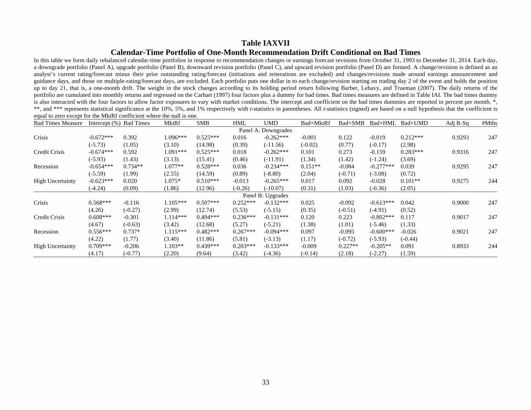
33

Table IAXVII Calendar-Time Portfolio of One-Month Recommendation Drift Conditional on Bad Times

In this table we form daily rebalanced calendar-time portfolios in response to recommendation changes or earnings forecast revisions from October 31, 1993 to December 31, 2014. Each day, a downgrade portfolio (Panel A), upgrade portfolio (Panel B), downward revision portfolio (Panel C), and upward revision portfolio (Panel D) are formed. A change/revision is defined as an analyst’s current rating/forecast minus their prior outstanding rating/forecast (initiations and reiterations are excluded) and changes/revisions made around earnings announcement and guidance days, and those on multiple-rating/forecast days, are excluded. Each portfolio puts one dollar in to each change/revision starting on trading day 2 of the event and holds the position up to day 21, that is, a one-month drift. The weight in the stock changes according to its holding period return following Barber, Lehavy, and Trueman (2007). The daily returns of the portfolio are cumulated into monthly returns and regressed on the Carhart (1997) four factors plus a dummy for bad times. Bad times measures are defined in Table IAI. The bad times dummy is also interacted with the four factors to allow factor exposures to vary with market conditions. The intercept and coefficient on the bad times dummies are reported in percent per month. *, **, and *** represents statistical significance at the 10%, 5%, and 1% respectively with t-statistics in parentheses. All t-statistics (signed) are based on a null hypothesis that the coefficient is equal to zero except for the MktRf coefficient where the null is one. Bad Times Measure Intercept (%) Bad Times

MktRf SMB HML UMD Bad×MktRf Bad×SMB Bad×HML Bad×UMD Adj R-Sq #Mths

Panel A: Downgrades Crisis -0.672*** 0.392 1.096*** 0.525*** 0.016 -0.262*** -0.001 0.122 -0.019 0.212*** 0.9293 247 (-5.73) (1.05) (3.10) (14.98) (0.39) (-11.56) (-0.02) (0.77) (-0.17) (2.98) Credit Crisis -0.674*** 0.592 1.091*** 0.525*** 0.018 -0.262*** 0.101 0.273 -0.159 0.283*** 0.9316 247 (-5.93) (1.43) (3.13) (15.41) (0.46) (-11.91) (1.34) (1.42) (-1.24) (3.69) Recession -0.654*** 0.734** 1.077** 0.528*** 0.036 -0.234*** 0.151** -0.084 -0.277*** 0.039 0.9295 247 (-5.59) (1.99) (2.55) (14.59) (0.89) (-8.80) (2.04) (-0.71) (-3.08) (0.72) High Uncertainty -0.623*** 0.020 1.075* 0.510*** -0.013 -0.265*** 0.017 0.092 -0.028 0.101** 0.9275 244 (-4.24) (0.09) (1.86) (12.96) (-0.26) (-10.07) (0.31) (1.03) (-0.36) (2.05)

Panel B: Upgrades Crisis 0.568*** -0.116 1.105*** 0.507*** 0.252*** -0.132*** 0.025 -0.092 -0.613*** 0.042 0.9000 247 (4.26) (-0.27) (2.99) (12.74) (5.53) (-5.15) (0.35) (-0.51) (-4.91) (0.52) Credit Crisis 0.608*** -0.301 1.114*** 0.494*** 0.236*** -0.131*** 0.120 0.223 -0.802*** 0.117 0.9017 247 (4.67) (-0.63) (3.42) (12.68) (5.27) (-5.21) (1.38) (1.01) (-5.46) (1.33) Recession 0.556*** 0.737* 1.115*** 0.482*** 0.267*** -0.094*** 0.097 -0.095 -0.600*** -0.026 0.9021 247 (4.22) (1.77) (3.40) (11.86) (5.81) (-3.13) (1.17) (-0.72) (-5.93) (-0.44) High Uncertainty 0.709*** -0.206 1.103** 0.439*** 0.203*** -0.133*** -0.009 0.227** -0.205** 0.091 0.8933 244 (4.17) (-0.77) (2.20) (9.64) (3.42) (-4.36) (-0.14) (2.18) (-2.27) (1.59)

34

Table IAXVII (Cont’d)

Bad Times Measure Intercept (%) Bad Times

MktRf SMB HML UMD Bad×MktRf Bad×SMB Bad×HML Bad×UMD Adj R-Sq #Mths Panel C: Downward Revisions

Crisis -0.483*** -0.226 1.170*** 0.459*** 0.231*** -0.244*** -0.058 0.097 -0.338** 0.039 0.8849 353 (-3.83) (-0.50) (5.22) (11.55) (5.07) (-9.23) (-0.80) (0.55) (-2.46) (0.46) Credit Crisis -0.509*** -0.041 1.181*** 0.455*** 0.232*** -0.246*** 0.005 0.448* -0.441*** 0.164* 0.8868 353 (-4.19) (-0.08) (6.12) (11.73) (5.19) (-9.58) (0.05) (1.80) (-2.68) (1.65) Recession -0.548*** 0.621 1.181*** 0.456*** 0.251*** -0.238*** 0.035 0.017 -0.348*** 0.051 0.8867 353 (-4.38) (1.61) (5.90) (11.20) (5.48) (-7.83) (0.43) (0.13) (-3.17) (0.81) High Uncertainty -0.565*** 0.317 1.150*** 0.425*** 0.186*** -0.275*** 0.008 0.195** -0.030 0.152*** 0.8874 350 (-3.74) (1.29) (3.62) (9.67) (3.32) (-9.04) (0.14) (1.99) (-0.35) (2.84)

Panel D: Upward Revisions Crisis 0.717*** 0.019 1.120*** 0.389*** 0.224*** -0.054* -0.121 -0.304 -0.459*** 0.133 0.8140 353 (4.92) (0.04) (3.18) (8.48) (4.25) (-1.77) (-1.46) (-1.48) (-2.89) (1.36) Credit Crisis 0.812*** -0.333 1.084** 0.378*** 0.203*** -0.068** 0.165 -0.024 -0.704*** 0.349*** 0.8183 353 (5.80) (-0.54) (2.48) (8.46) (3.95) (-2.31) (1.50) (-0.08) (-3.72) (3.07) Recession 0.810*** 0.255 1.068* 0.366*** 0.209*** -0.026 0.099 -0.174 -0.535*** -0.014 0.8108 353 (5.52) (0.56) (1.89) (7.65) (3.88) (-0.74) (1.04) (-1.13) (-4.15) (-0.19) High Uncertainty 0.811*** 0.036 1.147*** 0.299*** 0.137** -0.057 -0.190*** 0.318*** -0.014 0.079 0.8097 350 (4.54) (0.13) (3.00) (5.75) (2.07) (-1.59) (-2.84) (2.74) (-0.14) (1.25)

35

Panel A: Downward Revisions

Panel B: Upward Revisions

Figure IA1: Impact of earnings forecast revisions in bad times. The figure plots the mean two-day CAR and the influential probability of earnings forecast revisions (in percent). Panel A (Panel B) reports the evidence for downward revisions (upward revisions). The benchmark return for the CAR is the return from a characteristics-matched DGTW portfolio. The sample is from 1983 to 2014. A forecast revision is the analyst’s current one-quarter-ahead earnings forecast minus their prior outstanding forecast (i.e., initiations are excluded) scaled by price. Revisions made around earnings announcement and guidance days, and revisions on multiple-forecast days, are excluded. Influential revisions are those whose two-day CARs are in the same direction as the revision and is 1.96 times larger than expected based on the prior three-month idiosyncratic volatility of the stock (following Loh and Stulz (2011)). Bad times measures are as follows. Crisis: September to November 1987 (1987 crisis), August to December 1998 (LTCM), and July 2007 to March 2009 (Credit Crisis). Recession (NBER recessions): July 1990 to March 1991, March to November 2001, and December 2007 to June 2009. High Uncertainty represents the highest tercile (over the period 1983 to 2014) of the Baker, Bloom, and Davis (2016) uncertainty index.