international series of monographs
TRANSCRIPT

INTERNATIONAL SERIES OF MONOGRAPHSON PHYSICS
SERIES EDITORS
J. BIRMAN CITY UNIVERSITY OF NEW YORKS. F. EDWARDS UNIVERSITY OF CAMBRIDGER. FRIEND UNIVERSITY OF CAMBRIDGEM. REES UNIVERSITY OF CAMBRIDGED. SHERRINGTON UNIVERSITY OF OXFORDG. VENEZIANO CERN, GENEVA

International Series of Monographs on Physics
160. C. Barrabes, P.A. Hogan: Advanced general relativity–gravity waves, spinning particles, and black holes159. W. Barford: Electronic and optical properties of conjugated polymers, Second edition158. F. Strocchi: An introduction to non-perturbative foundations of quantum field theory157. K.H. Bennemann, J.B. Ketterson: Novel superfluids, Volume 2156. K.H. Bennemann, J.B. Ketterson: Novel superfluids, Volume 1155. C. Kiefer: Quantum gravity, Third edition154. L. Mestel: Stellar magnetism, Second edition153. R. A. Klemm: Layered superconductors, Volume 1152. E.L. Wolf: Principles of electron tunneling spectroscopy, Second edition151. R. Blinc: Advanced ferroelectricity150. L. Berthier, G. Biroli, J.-P. Bouchaud, W. van Saarloos, L. Cipelletti: Dynamical heterogeneities in glasses, colloids, and granular media149. J. Wesson: Tokamaks, Fourth edition148. H. Asada, T. Futamase, P. Hogan: Equations of motion in general relativity147. A. Yaouanc, P. Dalmas de Reotier: Muon spin rotation, relaxation, and resonance146. B. McCoy: Advanced statistical mechanics145. M. Bordag, G.L. Klimchitskaya, U. Mohideen, V.M. Mostepanenko: Advances in the Casimir effect144. T.R. Field: Electromagnetic scattering from random media143. W. Gotze: Complex dynamics of glass-forming liquids–a mode-coupling theory142. V.M. Agranovich: Excitations in organic solids141. W.T. Grandy: Entropy and the time evolution of macroscopic systems140. M. Alcubierre: Introduction to 3+1 numerical relativity139. A. L. Ivanov, S. G. Tikhodeev: Problems of condensed matter physics–quantum coherence phenomena in electron-hole and coupled
matter-light systems138. I. M. Vardavas, F. W. Taylor: Radiation and climate137. A. F. Borghesani: Ions and electrons in liquid helium135. V. Fortov, I. Iakubov, A. Khrapak: Physics of strongly coupled plasma134. G. Fredrickson: The equilibrium theory of inhomogeneous polymers133. H. Suhl: Relaxation processes in micromagnetics132. J. Terning: Modern supersymmetry131. M. Marino: Chern-Simons theory, matrix models, and topological strings130. V. Gantmakher: Electrons and disorder in solids129. W. Barford: Electronic and optical properties of conjugated polymers128. R. E. Raab, O. L. de Lange: Multipole theory in electromagnetism127. A. Larkin, A. Varlamov: Theory of fluctuations in superconductors126. P. Goldbart, N. Goldenfeld, D. Sherrington: Stealing the gold125. S. Atzeni, J. Meyer-ter-Vehn: The physics of inertial fusion123. T. Fujimoto: Plasma spectroscopy122. K. Fujikawa, H. Suzuki: Path integrals and quantum anomalies121. T. Giamarchi: Quantum physics in one dimension120. M. Warner, E. Terentjev: Liquid crystal elastomers119. L. Jacak, P. Sitko, K. Wieczorek, A. Wojs: Quantum Hall systems117. G. Volovik: The Universe in a helium droplet116. L. Pitaevskii, S. Stringari: Bose-Einstein condensation115. G. Dissertori, I.G. Knowles, M. Schmelling: Quantum chromodynamics114. B. DeWitt: The global approach to quantum field theory113. J. Zinn-Justin: Quantum field theory and critical phenomena, Fourth edition112. R.M. Mazo: Brownian motion–fluctuations, dynamics, and applications111. H. Nishimori: Statistical physics of spin glasses and information processing–an introduction110. N.B. Kopnin: Theory of nonequilibrium superconductivity109. A. Aharoni: Introduction to the theory of ferromagnetism, Second edition108. R. Dobbs: Helium three107. R. Wigmans: Calorimetry106. J. Kubler: Theory of itinerant electron magnetism105. Y. Kuramoto, Y. Kitaoka: Dynamics of heavy electrons104. D. Bardin, G. Passarino: The Standard Model in the making103. G. C. Branco, L. Lavoura, J.P. Silva: CP Violation102. T. C. Choy: Effective medium theory101. H. Araki: Mathematical theory of quantum fields100. L. M. Pismen: Vortices in nonlinear fields99. L. Mestel: Stellar magnetism98. K. H. Bennemann: Nonlinear optics in metals94. S. Chikazumi: Physics of ferromagnetism91. R. A. Bertlmann: Anomalies in quantum field theory90. P. K. Gosh: Ion traps87. P. S. Joshi: Global aspects in gravitation and cosmology86. E. R. Pike, S. Sarkar: The quantum theory of radiation83. P. G. de Gennes, J. Prost: The physics of liquid crystals73. M. Doi, S. F. Edwards: The theory of polymer dynamics69. S. Chandrasekhar: The mathematical theory of black holes51. C. Møller: The theory of relativity46. H. E. Stanley: Introduction to phase transitions and critical phenomena32. A. Abragam: Principles of nuclear magnetism27. P. A. M. Dirac: Principles of quantum mechanics23. R. E. Peierls: Quantum theory of solids
Advanced General Relativity
Gravity Waves, Spinning Particles,and Black Holes
C. BarrabesUniversite de Tours
P. A. HoganUniversity College Dublin
3

3
Great Clarendon Street, Oxford, OX2 6DP,United Kingdom
Oxford University Press is a department of the University of Oxford.It furthers the University’s objective of excellence in research, scholarship,
and education by publishing worldwide. Oxford is a registered trade mark ofOxford University Press in the UK and in certain other countries
c© Claude Barrabes, Peter A. Hogan 2013
The moral rights of the authors have been asserted
First Edition published in 2013Impression: 1
All rights reserved. No part of this publication may be reproduced, stored ina retrieval system, or transmitted, in any form or by any means, without the
prior permission in writing of Oxford University Press, or as expressly permittedby law, by licence or under terms agreed with the appropriate reprographics
rights organization. Enquiries concerning reproduction outside the scope of theabove should be sent to the Rights Department, Oxford University Press, at the
address above
You must not circulate this work in any other formand you must impose this same condition on any acquirer
Published in the United States of America by Oxford University Press198 Madison Avenue, New York, NY 10016, United States of America
British Library Cataloguing in Publication DataData available
Library of Congress Control Number: 2013938191
ISBN 978–0–19–968069–6
Printed and bound byCPI Group (UK) Ltd, Croydon, CR0 4YY
Links to third party websites are provided by Oxford in good faith andfor information only. Oxford disclaims any responsibility for the materials
contained in any third party website referenced in this work.

Preface
This book is aimed at students making the transition from a final year undergradu-ate course on general relativity, based on one of the many introductory texts, to aspecialized subfield of general relativity covered by an existing research monograph.We present a variety of topics under the general headings of gravitational waves invacuo and in a cosmological setting, equations of motion, and black holes, all hav-ing a clear physical relevance and a strong emphasis on space–time geometry. Thetopic of black hole physics is particularly extensive and so a selection of classical andquantum aspects, with suitable introduction, has been made with a view to comple-menting the recent text, Introduction to Black Hole Physics, by Frolov and Zelnikov(2011). Each chapter in this book could be used as a basis for an advanced under-graduate or early postgraduate project since our intention is to whet the appetite ofreaders who are exploring avenues into research in general relativity and who havealready accumulated the required technical knowledge. To be more specific we expectthe reader to have completed an introductory course on general relativity at the levelof Introducing Einstein’s Relativity by Ray d’Inverno (1992) and then to have supple-mented this material with additional techniques by individual study or in a taughtMSc programme. The additional technical knowledge required involves the Cartan cal-culus, the tetrad formalism including aspects of the Newman–Penrose formalism, theEhlers–Sachs theory of null geodesic congruences, and the Petrov classification of grav-itational fields, all of which are treated clearly and economically by S. Chandrasekhar(1983) in the mathematical preliminaries for The Mathematical Theory of Black Holes.For the geometry underpinning the cosmology treated here it would be hard to surpassthe lecture notes of G. F. R. Ellis (1971). The topics covered in this book are not indi-vidual applications of any one of these techniques. Our attitude to the techniques isto regard them as available to us in whole or in part (mainly in part) as each situationdemands. The presentation of each chapter is research monograph style rather thantextbook style in order to impress on interested students the need to present theirresearch in a clear and concise format. Our hope is that students with our taste ingeneral relativity will find a treasure trove here.

Acknowledgements
We thank the Universite de Tours, the Centre National de la Recherche Scientifique(CNRS), and the Ministere des Affaires Etrangeres for supporting our collaborationover many years. The work described in Chapter 3 on spinning particles was carriedout in collaboration with Mr. Shinpei Ogawa and we are grateful to him for his decis-ive contribution. We thank Dr. Loic Villain for his expert help in the production ofChapter 5.

Contents
1 Minkowskian space–time 11.1 Lorentz tansformations 11.2 Non-singular and singular Lorentz transformations 31.3 Infinitesimal Lorentz transformations 61.4 Geometrical construction of a gravitational wave 8
2 Plane gravitational waves 102.1 From linear approximation to colliding waves 102.2 Electromagnetic shock waves 172.3 Gravitational shock waves 212.4 High-frequency gravity waves 24
3 Equations of motion 283.1 Motivation 283.2 Example of a background space–time 333.3 Equations of motion of a Reissner–Nordstrom particle in first
approximation 373.4 Background space–time for a Kerr particle 393.5 Equations of motion of a Kerr particle in first approximation 453.6 Spinning test particles 53
4 Inhomogeneous aspects of cosmology 564.1 Plane-fronted gravitational waves with a cosmological constant 564.2 Perturbations of isotropic cosmologies 604.3 Gravitational waves 644.4 Cosmic background radiation 73
5 Black holes 795.1 Introduction: Basic properties of black holes 795.2 Collapsing null shells and trapped surface formation 865.3 Scattering properties of high-speed Kerr black holes 915.4 Inside the black hole 1035.5 Metric fluctuations and Hawking radiation 110
6 Higher dimensional black holes 1186.1 Brief outline of D-dimensional black holes 1196.2 Gibbons–Penrose isoperimetric inequality and the hoop
conjecture in D dimensions 1226.3 Light-like boost of higher dimensional black holes 124

viii Contents
Appendix A Notation 131
Appendix B Transport law for k along r =0 133
Appendix C Some useful scalar products 135
References 137
Index 142

1Minkowskian space–time
Space–time geometry was introduced into relativity theory in the classical paper byMinkowski (1909) [translated by Lorentz (1923)] and so we begin our presentationfrom the space–time viewpoint on general relativity by considering some aspects ofMinkowskian space–time. We discuss non-singular and singular Lorentz transforma-tions, infinitesimal Lorentz transformations, and exploit the similarities of the latterto electromagnetic fields. An elegant presentation, which has influenced us, is that ofTrautman et al. (1965). A natural generalization of the Lorentz transformations leadsto the geometrical construction of a gravitational wave.
1.1 Lorentz tansformations
The line-element of Minkowskian space–time, in rectangular Cartesian coordinatesand time, is given by
ds2 = dx 2 + dy2 + dz 2 − dt2 = ηij dx idx j . (1.1)
Here x i = (x , y , z , t) for i = 1, 2, 3, 4, respectively, and we use units in which the speedof light in vacuum is c = 1. In general Latin indices will take values 1, 2, 3, 4, theEinstein summation convention will apply, and (ηij ) = diag(1, 1, 1,−1) are the com-ponents of the Minkowskian metric tensor in coordinates x i with (ηij ) = (ηij )−1 =diag(1, 1, 1,−1) and Latin indices are raised and lowered as usual with ηij and ηij ,respectively.
There is a one-to-one correspondence between points of Minkowskian space–timewith position vectors x = (x , y , z , t) and 2 × 2 Hermitean matrices. Given a point xwe write the corresponding 2 × 2 Hermitean matrix in the form
A(x) =(−z + t x + iyx − iy z + t
). (1.2)
The standard way of demonstrating the action of the proper, orthochronous Lorentztransformations on Minkowskian space–time is to recognize that if U is a 2 × 2 mat-rix with complex entries and unit determinant (unimodular), and thus involving sixreal parameters, then the 2 × 2 matrix UA(x)U †, where U † denotes the Hermiteanconjugate of U , is itself a 2 × 2 Hermitean matrix and hence there exists a pointx′ = (x ′, y ′, z ′, t ′) of Minkowskian space–time for which
A(x′) = UA(x)U †. (1.3)

2 Minkowskian space–time
Calculating the determinants of both sides of this matrix equation immediatelyresults in
−x ′2 − y ′2 − z ′2 + t ′2 = −x 2 − y2 − z 2 + t2. (1.4)
Hence the transformation from x to x′, and vice versa, implicit in (1.3) is a Lorentztransformation which on more detailed examination is revealed to be proper (orienta-tion preserving) and orthochronous (preserving the time direction). We will henceforthrefer to such transformations simply as Lorentz transformations. On account of thequadratic dependence on U in (1.3) it is clear that there are two unimodular matrices±U corresponding to each Lorentz transformation. The matrices U are elements ofthe group SL(2,C) while the transformations from x to x′, and vice versa, constitutethe six-real-parameter proper, orthochronous Lorentz group.
Given a unimodular matrix U it is straightforward to calculate explicitly the cor-responding Lorentz transformation from (1.3). It is not quite so straightforward to cal-culate the two unimodular matrices corresponding to a given Lorentz transformationand so a little practice is useful. The reader can check that the diagonal matrices
U = ±(
e−iφ/2 00 eiφ/2
), (1.5)
correspond to the spatial rotation
x ′ = x cos φ + y sin φ, (1.6)y ′ = −x sin φ + y cos φ, (1.7)z ′ = z , (1.8)t ′ = t , (1.9)
whereas the matrices
U = ±(
cos θ2 sin θ
2− sin θ
2 cos θ2
), (1.10)
correspond to the spatial rotation
x ′ = x cos θ + z sin θ, (1.11)y ′ = y , (1.12)z ′ = −x sin θ + z cos θ, (1.13)t ′ = t . (1.14)
Also the diagonal matrices
U = ±(( 1−v
1+v
)−1/4 0
0( 1−v
1+v
)1/4
), (1.15)
correspond to the Lorentz boost
x ′ = x , (1.16)y ′ = y , (1.17)

Non-singular and singular Lorentz transformations 3
z ′ = γ(v) (z − v t), (1.18)t ′ = γ(v) (t − v z ), (1.19)
where γ(v) = (1 − v 2)−1/2 is the Lorentz factor, and the matrices
U = ± 1√2
( √γ(v) + 1 −
√γ(v) − 1
−√
γ(v) − 1√
γ(v) + 1
), (1.20)
correspond to the Lorentz boost
x ′ = γ(v) (x − v t), (1.21)y ′ = y , (1.22)z ′ = z , (1.23)t ′ = γ(v) (t − v x ). (1.24)
These one-parameter subgroups of the proper, orthochronous Lorentz group areuseful for illustrative purposes below. In the latter two examples the primed frameof reference is moving with constant 3-velocity v < 1 in the z -direction relative tothe unprimed frame in the case of (1.16)–(1.19) and in the x -direction relative to theunprimed frame in the case of (1.21)–(1.24).
1.2 Non-singular and singular Lorentz transformations
The position vector of a point on the future null-cone with vertex at the origin(0, 0, 0, 0) of the coordinates x i in Minkowskian space–time is given by
x = (x , y , z , t) with t > 0 and x 2 + y2 + z 2 = t2. (1.25)
This vector can be written in parametrized form as
x = t (sin θ cos φ, sin θ sin φ, cos θ, 1), (1.26)
with the polar angles θ, φ having the usual ranges 0 ≤ θ ≤ π and 0 ≤ φ < 2π. Thusa null direction on the future null-cone (1.25) is specified by the angles θ, φ. It isconvenient to use the complex number
ζ = eiφcotanθ
2, (1.27)
in place of the polar angles. The real and imaginary parts of this complex numberspecify the image in the equatorial plane of the stereographic projection from thenorth pole (corresponding to θ = 0) of a point on the unit 2-sphere. Thus (1.26) takesthe form
x = t(
ζ + ζ
1 + ζζ,i(ζ − ζ)1 + ζζ
,ζζ − 1ζζ + 1
, 1)
, (1.28)
with the bar denoting complex conjugation. Hence the points of the extended com-plex plane (the complex plane including the point at infinity ζ = ∞, with the lattercorresponding to θ = 0) are required to specify all of the null directions on the futurenull-cone (1.25). Clearly the point at infinity of the extended complex plane specifies

4 Minkowskian space–time
the generator t = z of the null-cone (1.25). Under a proper, orthochronous Lorentztransformation, (1.28) is transformed to another null position vector
x′ = t ′(
ζ ′ + ζ ′
1 + ζ ′ζ ′,i(ζ′ − ζ ′)1 + ζ′ζ ′
,ζ ′ζ ′ − 1ζ ′ζ ′ + 1
, 1)
, (1.29)
whose direction is specified by the complex number ζ′. Now
A(x) =2 t
1 + ζζ
(1 ζ
ζ ζζ
), (1.30)
with a similar equation for A(x′). The relationship between ζ ′ and ζ will tell us hownull directions on the null-cone are transformed under the Lorentz transformationsunder consideration. This information is readily obtained by substituting (1.30) andthe corresponding expression for A(x′) into (1.3) for any
U =(
α0 β0γ0 δ0
), (1.31)
where α0, β0, γ0, δ0 are complex numbers satisfying α0δ0 − β0γ0 = 1. Straightforwardalgebra reveals that
ζ′ =γ0 + δ0ζ
α0 + β0ζ. (1.32)
Such transformations constitute the fractional linear group of transformations of theextended complex plane. We have noted that there are two matrices U (differing only insign) corresponding to each Lorentz transformation whereas it is clear from (1.32) thatthere is a one-to-one correspondence between proper, orthochronous Lorentz trans-formations and fractional linear transformations. In fact these latter two groups oftransformations are isomorphic.
Fixed points of the transformation (1.32) correspond to null directions left invariantby Lorentz transformations. For a given Lorentz transformation the fixed points ζ aregiven by the roots of the quadratic equation
β0ζ2 + (δ0 − α0)ζ − γ0 = 0, (1.33)
over the field of complex numbers. Hence in general a proper, orthochronous Lorentztransformation leaves two null directions on the null-cone invariant. Such trans-formations are called non-singular. However it is obviously possible to have Lorentztransformations for which the roots of the quadratic equation (1.33) are equal. In thesecases only one null direction on the null-cone is left invariant. Such transformationsare called singular Lorentz transformations or null rotations.
The fixed points of the transformation (1.32) corresponding to the non-diagonalcase (1.10) above are ζ = ±i and the corresponding invariant null directions, obtainedfrom (1.28), are tangent to the null geodesic generators y = ±t of the null-cone withvertex (0, 0, 0, 0). The fixed points corresponding to (1.20) are ζ = ±1 and the corres-ponding invariant null directions are tangent to the lines x = ±t . The diagonal cases(1.5) and (1.15) both have β0 = 0 = γ0 and α0 �= δ0. In this case we see that (1.33) hasthe solution ζ = 0. Also rewriting (1.33) in the form
β0 + (δ0 − α0)ζ−1 − γ0ζ−2 = 0, (1.34)

Non-singular and singular Lorentz transformations 5
it follows that ζ = ∞ when β0 = 0 = γ0 and α0 �= δ0. Hence the invariant null directionsin the cases (1.5) and (1.15) are tangent to the lines z = ±t . Consequently all fourexamples in the previous section are non-singular Lorentz transformations. An exampleof a singular Lorentz transformation is
x ′ + iy ′ = x + iy + w (t + z ), (1.35)t ′ − z ′ = t − z + ww(t + z ) + w(x − iy) + w(x + iy), (1.36)t ′ + z ′ = t + z , (1.37)
where w �= 0 (w = 0 for the identity transformation) is a complex number with complexconjugate w . In this form it is easy to check that (1.4) is satisfied. The correspondingmatrices U are found to be
U = ±(
1 w0 1
). (1.38)
The unique fixed point of (1.32) is thus ζ = 0 and the corresponding invariant null dir-ection is tangent to the line z = −t . The transformations (1.35)–(1.37) constitute anAbelian, two-(real)-parameter subgroup of the proper, orthochronous Lorentz group.It is interesting to transform (1.35)–(1.37) from the coordinates (x , y , z , t) to thecoordinates (ξ, η, r , u) via
ξ =x
z + t, (1.39)
η =y
z + t, (1.40)
r = z + t , (1.41)
u = −12(z − t) − 1
2(x 2 + y2)
z + t. (1.42)
Now (1.35)–(1.37) takes the simpler form
ξ′ + iη′ = ξ + iη + w , r ′ = r , u ′ = u. (1.43)
Even more revealing is to write the Minkowskian line-element (1.1) in the coordinates(ξ, η, r , u). This results in
ds2 = r 2(dξ2 + dη2) − 2 du dr , (1.44)
which was first given by Ivor Robinson (see Rindler and Trautman (1987)) as abyproduct of his study of the Schwarzschild line-element in the limit of the massm → +∞. It is immediate from (1.44) that r = 0 is a null geodesic with u an affineparameter along it and that (1.43) is a Lorentz transformation which leaves this nullgeodesic invariant. This observation by Robinson is of great significance in the historyof singular Lorentz transformations [see Synge (1965), p.viii].
Robinson’s interesting limit of the Schwarzschild solution referred to above isobtained by first writing the Schwarzschild line-element in the form (a more commonform of the Schwarzschild line-element can be found in (3.1) below)
ds2 =r 2(dξ2 + dη2)
cosh2 λ ξ− 2 du dr −
(λ2 − 2
r
)du2, (1.45)

6 Minkowskian space–time
with
λ = m−1/3, (1.46)
and then taking the limit λ → 0 (equivalently m → +∞) to arrive at the line-element
ds2 = r 2(dξ2 + dη2) − 2 du dr +2r
du2. (1.47)
This is the flat space–time line-element (1.44) with the addition of a term (the finalterm) which is singular at r = 0. The reader may like to show that, with a suitablecoordinate transformation, it can be put in the vacuum Kasner (1925) form:
ds2 = T 4/3(dX 2 + dY 2) + T−2/3dZ 2 − dT 2. (1.48)
1.3 Infinitesimal Lorentz transformations
A convenient way to introduce infinitesimal Lorentz transformations in the formalismabove is via the approximately unimodular matrices
U = ±(
1 + ε(a1 + ia2) + O(ε2) ε(b1 + ib2) + O(ε2)
ε(c1 + ic2) + O(ε2) 1 − ε(a1 + ia2) + O(ε2)
). (1.49)
Here ε is a small real parameter controlling the approximation where we neglect O(ε2)terms but keep a note of their presence. Also a1, a2, b1, b2, c1, c2 are six real numbers.Now using (1.3) the corresponding infinitesimal Lorentz transformation can be writtenin the form (for i = 1, 2, 3, 4)
x ′i = x i + εLij x
j + O(ε2), (1.50)
where x ′i = (x ′, y ′, z ′, t ′) and
(Lij ) =
⎛⎜⎜⎜⎜⎜⎝
0 −2a2 b1 − c1 b1 + c1
2a2 0 b2 + c2 b2 − c2
−(b1 − c1) −(b2 + c2) 0 −2a1
b1 + c1 b2 − c2 −2a1 0
⎞⎟⎟⎟⎟⎟⎠ , (1.51)
with the upper index on L indicating the rows and the lower index indicating thecolumns in this matrix. Let x i = x i(s) be a time-like world line in Minkowskian space–time, with s the arc length or proper-time along it. Let ui = dx i/ds and then ηij ui uj =ui ui = −1 for all s. Thus ui is the 4-velocity of the particle with world line x i = x i (s).Since ui ui is conserved along this world line it follows that ui (s1) and ui(s2), fors1 �= s2, must be related by a Lorentz transformation. In particular ui(s + ε) and ui (s),for small ε, must be related by an infinitesimal Lorentz transformation for which theentries in the matrix (1.51) depend upon s. Thus
ui (s + ε) = ui (s) + εLij (s)u
j (s) + O(ε2). (1.52)
Infinitesimal Lorentz transformations 7
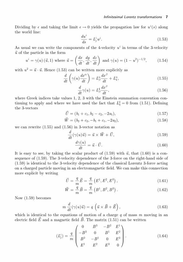
Dividing by ε and taking the limit ε → 0 yields the propagation law for ui(s) alongthe world line:
dui
ds= Li
j uj . (1.53)
As usual we can write the components of the 4-velocity ui in terms of the 3-velocity�u of the particle in the form
ui = γ(u) (�u, 1) where �u =(
dxdt
,dydt
,dzdt
)and γ(u) = (1 − u2)−1/2, (1.54)
with u2 = �u · �u. Hence (1.53) can be written more explicitly asddt
(γ(u)
dxα
dt
)= Lα
β
dx β
dt+ Lα
4 , (1.55)
ddt
γ(u) = L4β
dx β
dt, (1.56)
where Greek indices take values 1, 2, 3 with the Einstein summation convention con-tinuing to apply and where we have used the fact that L4
4 = 0 from (1.51). Definingthe 3-vectors
�U = (b1 + c1, b2 − c2,−2a1), (1.57)�W = (b2 + c2,−b1 + c1,−2a2), (1.58)
we can rewrite (1.55) and (1.56) in 3-vector notation asddt
(γ(u)�u) = �u × �W + �U , (1.59)
dγ(u)dt
= �u · �U . (1.60)
It is easy to see, by taking the scalar product of (1.59) with �u, that (1.60) is a con-sequence of (1.59). The 3-velocity dependence of the 3-force on the right-hand side of(1.59) is identical to the 3-velocity dependence of the classical Lorentz 3-force actingon a charged particle moving in an electromagnetic field. We can make this connectionmore explicit by writing
�U =qm
�E =qm(E 1,E 2,E 3) , (1.61)
�W =qm
�B =qm(B 1,B 2,B 3) . (1.62)
Now (1.59) becomes
mddt
(γ(u)�u) = q(�u × �B + �E
), (1.63)
which is identical to the equations of motion of a charge q of mass m moving in anelectric field �E and a magnetic field �B . The matrix (1.51) can be written
(Lij ) =
qm
⎛⎜⎜⎜⎝
0 B3 −B2 E 1
−B3 0 B1 E 2
B 2 −B1 0 E 3
E 1 E 2 E 3 0
⎞⎟⎟⎟⎠ . (1.64)

8 Minkowskian space–time
We note that if we neglect O(ε) terms then with U given by (1.49) the fixed nulldirections of the infinitesimal Lorentz transformations generating the transport of ui
along the time-like world line are given by ζ(s) such that
(b1 − ib2)ζ2 − 2(a1 − ia2)ζ − (c1 − ic2) = 0. (1.65)
In terms of the vectors �E and �B we have (ignoring a factor of q/m which is unnecessaryhere)
a1 + ia2 = −12(E 3 + iB 3) , (1.66)
b1 + ib2 =12(E 1 + iE 2)+
i2(B 1 + iB2) , (1.67)
c1 + ic2 =12(E 1 − iE 2)+
i2(B 1 − iB2) . (1.68)
Hence we see that the roots of (1.65) are equal if and only if
|�E |2 − |�B |2 = 0 and �E · �B = 0, (1.69)
indicating that the time-like world line of the charged mass is generated by a successionof infinitesimal singular Lorentz transformations provided the charge is moving in apurely radiative electromagnetic field. Further information, such as the transformationlaws for �E and �B under the Lorentz boost (1.21)–(1.24), can be deduced from theconstruction given here.
1.4 Geometrical construction of a gravitational wave
With ξ + iη =√
2Z we can rewrite (1.39)–(1.42) equivalently as
x + iy = r√
2Z , x − iy = r√
2 Z , z + t = r and − z + t = 2 u + 2 r Z Z , (1.70)
with the bar as usual denoting complex conjugation. Thus the line-element (1.44) takesthe form
ds2 = 2 r2dZ dZ − 2 du dr . (1.71)
It is easy to check now that u = constant are null cones with vertices on the nullgeodesic r = 0. When the proper, orthochronous Lorentz transformation (1.3), withU given by (1.31), is written in terms of the coordinates Z , Z , r , u it can be simplifiedto read
r ′ = 2 γ0γ0u + r |√
2 γ0 Z + δ0|2, (1.72)
r ′ Z ′ =√
2 α0 γ0 u + r(√
2 γ0 Z + δ0
) ( 1√2
β0 + α0 Z)
, (1.73)
u ′ =u r
2 γ0 γ0 u + r |√
2 γ0 Z + δ0|2. (1.74)
As a first step in generalizing this transformation let
f (Z ) =1√2β0 + α0 Z
δ0 +√
2 γ0 Z, (1.75)

Geometrical construction of a gravitational wave 9
and, denoting the derivative of this with a prime, we can write (1.72)–(1.74) in theform (Hogan, 1994)
r ′ =r|f ′|
(1 +
u4 r
∣∣∣∣ f ′′f ′
∣∣∣∣2)
, (1.76)
u ′ = u |f ′|(
1 +u4 r
∣∣∣∣ f ′′f ′
∣∣∣∣2)−1
, (1.77)
Z ′ = f (Z ) − u2 r
f ′ f ′′
f ′
(1 +
u4 r
∣∣∣∣ f ′′f ′
∣∣∣∣2)−1
. (1.78)
Now assume that f (Z ) is an arbitrary analytic function and calculate the line-elementfrom
ds2 = 2 r ′2dZ ′ dZ ′ − 2 du ′ dr ′,
= 2 r 2∣∣∣dZ − u
2 rH (Z ) dZ
∣∣∣2 − 2 du dr , (1.79)
where
H (Z ) =f ′′′
f ′− 3
2
(f ′′
f ′
)2
. (1.80)
The analytic function (1.80) vanishes if and only if the function f (Z ) is fractional linearas in (1.75). Penrose’s (1972) ‘spherical’ impulsive gravitational wave having as historyin space–time the future null-cone u = 0 is obtained from this simply by replacing thecoefficient u of H in (1.79) by u ϑ(u) where ϑ(u) is the Heaviside step function whichis unity for u > 0 and vanishes for u < 0. The Ricci tensor, calculated with the metrictensor given via the line-element (1.79) with u replaced by u ϑ(u), vanishes, indicatingthat we have a vacuum space–time in particular on u = 0 (the space–time is of courseMinkowskian for u > 0 and for u < 0). There is only one Newman–Penrose componentof the Riemann curvature tensor and it is
Ψ4 =1
2 rH (Z ) δ(u). (1.81)
This fact indicates that the Riemann tensor is type N (radiative) in the Petrov classi-fication with ∂/∂r as degenerate principal null direction. The profile is a Dirac deltafunction which is singular on the history of the wave u = 0 and the field is also sin-gular on the null geodesic r = 0 which is a generator of the null-cone u = 0. Thus thewavefront has a singular point on it and so the wave is not strictly spherical. Furtherdetails including the construction of this wave using a ‘cut and paste’ approach canbe found in Penrose (1972) and Barrabes and Hogan (2003b) and references therein.

2Plane gravitational waves
Most introductory texts on general relativity present plane gravitational waves ofarbitrary profile as solutions of Einstein’s vacuum field equations in the linear approx-imation. Starting in this way we lead the reader through a sequence of gaugetransformations to a metric tensor which is an exact solution of the vacuum fieldequations. We specialize to impulsive plane gravitational waves having a Dirac deltafunction profile and then give a simple derivation of the Khan–Penrose solution ofEinstein’s vacuum field equations describing the gravitational field following the head-on collision of such plane waves. By comparison the head-on collision of electromagneticshock waves, having a Heaviside step function profile, leading to the Bell–Szekeressolution of the vacuum Einstein–Maxwell field equations, is described and the corres-ponding solution of Einstein’s field equations for colliding gravitational shock wavesis also given. Finally we consider high-frequency gravitational waves propagating ina vacuum and examine the similarities between plane and approximately sphericalfronted waves.
2.1 From linear approximation to colliding waves
In order to establish notation for this very familiar topic we begin by writing themetric tensor components as small perturbations of the Minkowskian metric tensorthus:
gij = ηij + γij , (2.1)
where ηij is given via (1.1) and γij = γji with γij = γij (x , y , z , t). We can consider γijas the components of a tensor field on Minkowskian space–time with metric tensorhaving components ηij . Now define the star conjugate of γij by
γ∗ij = γij −
12ηij γ, (2.2)
with γ = ηij γij . If γ∗ij satisfies the coordinate conditions
ηjkγ∗ij ,k = 0, (2.3)
with the comma denoting partial differentiation with respect to xk , then Einstein’svacuum field equations in the linear approximation reduce to the 4-dimensional waveequation
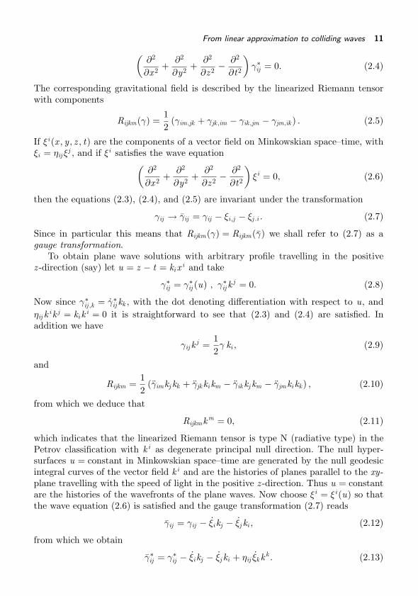
From linear approximation to colliding waves 11
(∂2
∂x 2 +∂2
∂y2 +∂2
∂z 2 − ∂2
∂t2
)γ∗
ij = 0. (2.4)
The corresponding gravitational field is described by the linearized Riemann tensorwith components
Rijkm(γ) =12
(γim,jk + γjk ,im − γik ,jm − γjm,ik ) . (2.5)
If ξi (x , y , z , t) are the components of a vector field on Minkowskian space–time, withξi = ηij ξ
j , and if ξi satisfies the wave equation(∂2
∂x 2 +∂2
∂y2 +∂2
∂z 2 − ∂2
∂t2
)ξi = 0, (2.6)
then the equations (2.3), (2.4), and (2.5) are invariant under the transformation
γij → γij = γij − ξi ,j − ξj .i . (2.7)
Since in particular this means that Rijkm(γ) = Rijkm(γ) we shall refer to (2.7) as agauge transformation.
To obtain plane wave solutions with arbitrary profile travelling in the positivez -direction (say) let u = z − t = ki x i and take
γ∗ij = γ∗
ij (u) , γ∗ij k
j = 0. (2.8)
Now since γ∗ij ,k = γ∗
ij kk , with the dot denoting differentiation with respect to u, andηij k i k j = ki k i = 0 it is straightforward to see that (2.3) and (2.4) are satisfied. Inaddition we have
γij k j =12γ ki , (2.9)
and
Rijkm =12
(γimkj kk + γjk ki km − γik kj km − γjmki kk ) , (2.10)
from which we deduce that
Rijkmkm = 0, (2.11)
which indicates that the linearized Riemann tensor is type N (radiative type) in thePetrov classification with k i as degenerate principal null direction. The null hyper-surfaces u = constant in Minkowskian space–time are generated by the null geodesicintegral curves of the vector field k i and are the histories of planes parallel to the xy-plane travelling with the speed of light in the positive z -direction. Thus u = constantare the histories of the wavefronts of the plane waves. Now choose ξi = ξi(u) so thatthe wave equation (2.6) is satisfied and the gauge transformation (2.7) reads
γij = γij − ξi kj − ξj ki , (2.12)
from which we obtain
γ∗ij = γ∗
ij − ξi kj − ξj ki + ηij ξk kk . (2.13)

12 Plane gravitational waves
We note that since γ∗i3 + γ∗
i4 = γ∗ij k
j = 0 we have γ∗i3 + γ∗
i4 = γ∗ij k
j = 0. In view of (2.13)we see that we can choose ξ1(u) such that ξ1 = γ∗
13 = −γ∗14 in order to have γ∗
13 =0 = γ∗
14. We can also choose ξ2(u) such that ξ2 = γ∗23 = −γ∗
24 to have γ∗23 = 0 = γ∗
24.Finally it is convenient to choose ξ3(u) and ξ4(u) so that ξ3 − ξ4 = γ∗
33 = −γ∗34 and
ξ3 + ξ4 = −(γ∗11 + γ∗
22)/2. The latter choices for ξ3 and ξ4 will ensure that γ∗ij is trace-
free and so γ∗ij = γij . Now, dropping the bars, we can say that without loss of generality
γij (u) for plane waves travelling in the positive z -direction has the property that allcomponents can be taken to vanish except for γ11 = −γ22 and γ12. The reader canverify that a further gauge transformation results in
γij = γij − λi ,j − λj ,i = H kikj , (2.14)
and
H =12γ11(x 2 − y2) + γ12 x y , (2.15)
with
λ1 =12{γ11 x + γ12 y}, (2.16)
λ2 =12{γ12 x − γ11 y}, (2.17)
λ3 = −14{γ11 (x 2 − y2) + 2 γ12 x y}, (2.18)
λ4 =14{γ11 (x 2 − y2) + 2 γ12 x y}. (2.19)
Clearly λi satisfies the wave equation (2.6). All components of λi are harmonic func-tions of x and y . Now the line-element of the space–time with metric tensor (2.1) canbe written (dropping the hat in (2.14))
ds2 = dx 2 + dy2 + dz 2 − dt2 + H du2, (2.20)
where du = kidx i . With u = z − t and −2 v = z + t this takes the slightly simplerform
ds2 = dx 2 + dy2 − 2 du dv + H du2. (2.21)
Remarkably the metric tensor given by this line-element is an exact solution ofEinstein’s vacuum field equations and the space–time is a model of the gravitationalfield due to a train of plane gravitational waves of arbitrary profile. The fact that thereare two arbitrary functions of u in H given by (2.15) demonstrates that the waves havetwo degrees of freedom of polarization just like plane electromagnetic waves.
We shall next transform the line-element (2.21) into a form in which the metrictensor components are independent of x and y . This is known as the Rosen (1937)form and, although the transformation can be given for the general case of γ11 �= 0and γ12 �= 0 [see, for example, Futamase and Hogan (1993)] we will consider here thespecial case of γ12 = 0. The coordinate transformation is (x , y , u, v) → (x ′, y ′, u ′, v ′)given by
x = F (u ′) x ′, (2.22)
From linear approximation to colliding waves 13
x = G(u ′) y ′, (2.23)u = u ′, (2.24)
v = v ′ +12F F x ′2 +
12G G y ′2, (2.25)
with the dot indicating differentiation with respect to u ′, and F (u ′),G(u ′) chosen tosatisfy
F − 12γ11 F = 0 and G +
12γ11 G = 0. (2.26)
The resulting Rosen form of the line-element (2.20) is
ds2 = F 2dx ′2 + G2dy ′2 − 2 du ′ dv ′. (2.27)
From now on we shall drop the primes on the coordinates in (2.26) and (2.27).Our freedom to choose the function 1
2 γ11 corresponds to our freedom to choose theprofile of the plane gravitational waves. For a single plane impulsive wave we shouldchoose 1
2 γ11 = δ(u), where δ(u) is the Dirac delta function which is singular on thenull hypersurface u = 0. With this choice in (2.26) we find that
F = 1 + u ϑ(u) and G = 1 − u ϑ(u), (2.28)
where ϑ(u) is the Heaviside step function which is equal to unity for u > 0 and vanishesfor u < 0. Now the line-element reads
ds2 = (1 + u ϑ(u))2dx 2 + (1 − u ϑ(u))2dy2 − 2 du dv . (2.29)
The metric given via this line-element is a solution of the vacuum field equationsRij = 0, where Rij are the components of the Ricci tensor. These field equations holdeverywhere, in particular on u = 0. The non-identically vanishing components of theRiemann tensor are proportional to δ(u) (thus Rijkl ∝ δ(u)). Hence we see that ifu < 0 or u > 0 then (2.29) is the line-element of Minkowskian space–time (vanishingRiemann tensor) and the Riemann tensor is singular on the null hypersurface historyu = 0 of the plane impulsive gravitational wave. In the space–time with line-element(2.29) there are two families of intersecting null hypersurfaces, u = constant and v =constant. Thus a plane, homogeneous, impulsive gravitational wave propagating in theopposite direction to that with history u = 0 above, with history in space–time v = 0,is described by a space–time with line-element
ds2 = (1 + v ϑ(v))2dx 2 + (1 − v ϑ(v))2dy2 − 2 du dv . (2.30)
Following the collision of two such waves we have u > 0 and v > 0 and the gravitationalfield is described by a vacuum space–time with line-element of the form (Khan andPenrose 1971, Szekeres 1970, 1972)
ds2 = e−U+V dx 2 + e−U−V dy2 − 2 e−M du dv , (2.31)
where U ,V ,M are functions of u and v . A simple but important observation aboutthis line-element is that under the coordinate transformation u → u(u) and v → v(v)

14 Plane gravitational waves
the form of the line-element is unchanged but the function M is transformed to Mwith
e−M = e−M dudu
dvdv
. (2.32)
The region of space–time u < 0 has line-element (2.30) and the region of space–timev < 0 has line-element (2.29). The space–time model of the vacuum gravitational fieldafter the collision has line-element of the form (2.31) with u > 0, v > 0 and with thefunctions U ,V ,M satisfying the following boundary conditions:
On v = 0, u > 0:
U = − log(1 − u2) , V = log(
1 + u1 − u
), M = 0 ; (2.33)
On u = 0, v > 0:
U = − log(1 − v 2) , V = log(
1 + v1 − v
), M = 0. (2.34)
Clearly these conditions ensure continuity of the metric tensor components on theboundaries v = 0, u > 0 and u = 0, v > 0 of the post-collision region of the space–time. With subscripts denoting partial derivatives, the vacuum field equations to besatisfied by the functions U ,V ,M in (2.31) read:
Uuv = Uu Uv , (2.35)
2Vuv = Uu Vv + Uv Vu , (2.36)
2Uuu = U 2u + V 2
u − 2Uu Mu , (2.37)
2Uvv = U 2v + V 2
v − 2Uv Mv , (2.38)
2Muv = Vu Vv − Uu Uv . (2.39)
The first of these equations can be written (e−U )uv = 0 and this is easy to integrateto
e−U = f (u) + g(u), (2.40)
and so to satisfy (2.33) and (2.34) we have
e−U = 1 − u2 − v 2. (2.41)
Now V is calculated from (2.36) while M is given by (2.37) and (2.38) with (2.39) theintegrability condition (or the consistency condition) for (2.37) and (2.38). To solve(2.36) we write it in a way that suggests a simplifying assumption (see Barrabes andHogan (2003b)), namely,
2∂2
∂u ∂vlog
(Vv
Vu
)=(
UvVu
Vv
)v−(
UuVv
Vu
)u. (2.42)
The simplifying assumption that this equation suggests is to try the separation ofvariables
Vv
Vu=
A(u)B(v)
. (2.43)

From linear approximation to colliding waves 15
To determine the functions A(u) and B(v) we only require the boundary values of Vuand Vv which we can calculate from (2.36). For example (2.36) evaluated at v = 0 andusing (2.33) and (2.41) yields the differential equation
ddu
(Vv )v=0 =u
1 − u2 (Vv )v=0, (2.44)
and so
(Vv )v=0 =a0√
1 − u2, (2.45)
with a0 a constant of integration. But (2.34) gives
(Vv )u=0 =2
1 − v 2 , (2.46)
and thus for (2.45) and (2.46) to agree when v = 0 and when u = 0 we must havea0 = 2. Hence
(Vv )v=0 =2√
1 − u2. (2.47)
Similarly we have
(Vu)v=0 =2
1 − u2 and (Vu)u=0 =2√
1 − v 2. (2.48)
Now evaluating (2.43) at u = 0 and at v = 0 will determine the functions A(u) andB(v). We easily find that
Vv
Vu=
√1 − u2
√1 − v 2
. (2.49)
Introducing the coordinates u, v via
u = sin−1 u and v = sin−1 v , (2.50)
we see that (2.49) becomes the first-order wave equation
Vu = Vv , (2.51)
which immediately integrates to V = V (u + v). When v = 0 we have v = 0 and, by(2.33) and (2.50), we have
V = log(
1 + sin u1 − sin u
)when v = 0. (2.52)
Hence for u > 0 and v > 0 we arrive at
V (u, v) = log(
1 + sin(u + v)1 − sin(u + v)
)= log
{(cos u + sin vcos u − sin v
)(cos v + sin ucos v − sin u
)}. (2.53)
The equality of the arguments of the logarithms here is a nice trigonometric identityto establish. In terms of the barred coordinates we see that (2.41) reads
e−U = cos(u − v) cos(u + v), (2.54)

16 Plane gravitational waves
from which it follows that U satisfies the second-order wave equation
Uuu = Uvv . (2.55)
The reader can readily check that this equation is equivalent to the vanishing of theright-hand side of (2.42). To calculate M we first calculate M , using the field equationswritten in terms of the barred coordinates and M , and then obtain M from (2.32). Itis convenient to define
Q = M +12
U , (2.56)
and then (2.37) and (2.38) in the barred variables reduce to
Qu = Qv = 2 tan(u + v). (2.57)
We note at this point that (2.39) in the barred variables reads
Quv =12
Vu Vv , (2.58)
and this is now satisfied on account of (2.57) and V given by (2.53). To solve (2.57)we need the boundary conditions: When u = 0 we must have Q = −2 log cos v andwhen v = 0 we must have Q = −2 log cos u, which follow easily from the boundaryconditions above expressed in terms of the barred coordinates. We thus obtain from(2.57) the solution
Q = −2 log cos(u + v). (2.59)
With this and (2.47) and (2.49) we have
eM =(
cos(u − v)cos3(u + v)
)1/2
. (2.60)
Now (2.32) with (2.50) yields
e−M = e− 32 U {cos2(u − v) cos u cos v}−1. (2.61)
The functions U ,V ,M in (2.31) for u > 0, v > 0 are given by (2.54), (2.53), and(2.61), respectively. Writing them in terms of the coordinates u, v we have U given by(2.41), V is now
eV =
(√1 − u2 + v√1 − u2 − v
)(√1 − v 2 + u√1 − v 2 − u
), (2.62)
and M is given by
e−M =(1 − u2 − v 2)3/2
{√
1 − u2√
1 − v 2 + u v}2√
1 − u2√
1 − v 2. (2.63)
When (2.41), (2.62), and (2.63) are substituted into the line-element (2.31) we arrive atthe Khan–Penrose (1971) solution of Einstein’s vacuum field equations. This expressionfor the line-element is valid for u > 0, v > 0. To obtain an expression valid for all u, vwe simply replace u and v in (2.41), (2.62), and (2.63) by u+ = u ϑ(u) and v+ = v ϑ(v),
Electromagnetic shock waves 17
respectively. The reader can verify that the Khan–Penrose solution for u > 0, v > 0has a singularity in the curvature tensor at e−U = 1 − u2 − v 2 = 0 and so the solutionis valid in the region u > 0, v > 0 only up to the quadrant of the circle u2 + v 2 = 1.Further properties of this solution can be found in Griffiths (1991).
2.2 Electromagnetic shock waves
Henceforth in this chapter we shall only consider line-elements of the simple form(with M = 0)
ds2 = e−U+V dx 2 + e−U−V dy2 − 2 du dv , (2.64)
where U and V are in general functions of u and v . We can write (2.64) as
ds2 = (ϑ1)2 + (ϑ2)2 − 2ϑ3ϑ4 = gabϑaϑb , (2.65)
with the basis 1-forms defined by
ϑ1 = e(−U+V )/2dx = ϑ1, (2.66)ϑ2 = e−(U+V )/2dy = ϑ2, (2.67)ϑ3 = du = −ϑ4, (2.68)ϑ4 = dv = −ϑ3. (2.69)
These 1-forms define a half-null tetrad. The constants gab are the components of themetric tensor on this tetrad and tetrad indices are lowered [as in the second equalitiesin (2.66)–(2.69)] and raised using gab and its inverse gab = gab , respectively. Withsubscripts on U ,V denoting partial differentiation the non-vanishing components ofthe Riemann curvature tensor on the half-null tetrad are
R1212 =12
(UuUv − VuVv ) , (2.70)
R1313 =12
(Uuu − Vuu) −14
(Uu − Vu)2, (2.71)
R1314 =12
(Uuv − Vuv ) −14
(Uu − Vu) (Uv − Vv ) , (2.72)
R2323 =12
(Uuu + Vuu) −14
(Uu + Vu)2, (2.73)
R2324 =12
(Uuv + Vuv ) −14
(Uu + Vu) (Uv + Vv ) , (2.74)
R1414 =12
(Uvv − Vvv ) −14
(Uv − Vv )2, (2.75)
R2424 =12
(Uvv + Vvv ) −14
(Uv + Vv )2 . (2.76)
The non-identically vanishing components of the Ricci tensor on the half-null tetrad,Rab = gcd Racbd , are given by
R11 = −Uuv + Uu Uv + Vuv −12
(UuVv + UvVu) , (2.77)

18 Plane gravitational waves
R22 = −Uuv + Uu Uv − Vuv +12
(UuVv + UvVu) , (2.78)
R33 = Uuu − 12(U 2
u + V 2u), (2.79)
R34 = Uuv −12
(UuUv + VuVv ) , (2.80)
R44 = Uvv −12(U 2
v + V 2v). (2.81)
The Weyl conformal curvature tensor components Cabcd on the tetrad are related tothe components Rabcd of the Riemann curvature tensor on the tetrad, the componentsRab of the Ricci tensor on the tetrad, and the Ricci scalar R = gab Rab by the formula
Cabcd = Rabcd +12
(gad Rbc + gbc Rad − gac Rbd − gbd Rac)
+16
R (gac gbd − gad gbc) . (2.82)
We note that the Newman–Penrose (1962) components ΨA for A = 0, 1, 2, 3, 4 of theWeyl conformal curvature tensor are related to the tetrad components of the Riemannand Ricci tensors by
Ψ0 = R1313 −12R33 + iR1323, (2.83)
Ψ1 =1√2
(R3431 + iR3432) −1
2√
2(R31 + iR32) , (2.84)
Ψ2 =12
(R3434 + iR3412 − R34 +
16R)
, (2.85)
Ψ3 =1√2
(R3414 − iR3424 +
12R41 +
12iR42
), (2.86)
Ψ4 = R1414 −12R44 − iR1424, (2.87)
with R = R11 + R22 − 2R34.A quick perusal of the passage from (2.21) to (2.27) will reveal that a similar
coordinate transformation applied to (2.21) when
H = A(u) (x 2 + y2), (2.88)
will also lead, after dropping the primes, to a homogeneous metric tensor (havingcomponents independent of x and y) given by the line-element
ds2 = F 2dx 2 + G2dy2 − 2du dv , (2.89)
where F (u) and G(u) satisfy
F − AF = 0 and G − AG = 0. (2.90)
A simple solution corresponding to the choice A(u) = −a2ϑ(u), where ϑ(u) is theHeaviside step function used above and a is a constant, is given by
F (u) = G(u) = cos a u+, (2.91)

Electromagnetic shock waves 19
where u+ = u ϑ(u). In differentiating this function we note that dϑ(u)/du = δ(u) andalso f (u) δ(u) = f (0) δ(u) and ϑ2(u) = ϑ(u). The resulting line-element
ds2 = cos2 au+(dx 2 + dy2) − 2du dv , (2.92)
is interesting from a physical point of view. It fits into the expression (2.64) andtherefore the calculation of the Ricci tensor is easily carried out using the formulae(2.77)–(2.81) to obtain
Rab = 2a2ϑ(u)δ3a δ3
b . (2.93)
These are the vacuum Einstein–Maxwell field equations
Rab = 2Eab , (2.94)
with the electromagnetic energy tensor
Eab = FacFbc − 1
4gab Fcd F cd , (2.95)
derived from the Maxwell 2-form
F =12
Fab ϑa ∧ ϑb = a ϑ(u)ϑ1 ∧ ϑ3. (2.96)
It is simple to check that this 2-form is a solution of Maxwell’s vacuum field equationsdF = 0 = d∗F , where d is the exterior derivative and the star indicates the Hodgedual. This Maxwell field is type N (the radiative type) in the Petrov classification of2-forms and describes electromagnetic radiation with propagation direction in space–time given by the vector field ∂/∂v . The profile of the wave is the step function andso we have here an electromagnetic shock wave.
The head-on collision of two electromagnetic shock waves is described by the Bell–Szekeres (1974) solution of the vacuum Einstein–Maxwell field equations with line-element
ds2 = cos2(au+ + bv+) dx 2 + cos2(au+ − bv+) dy2 − 2 du dv , (2.97)
where b is a constant and v+ = v ϑ(v). When v < 0 this coincides with (2.92) and whenu < 0 it describes the second incoming electromagnetic shock wave with propagationdirection in space–time given by the vector field ∂/∂u. The region of space–time corres-ponding to u < 0 and v < 0 is Minkowskian while the region u > 0, v > 0 correspondsto the post-collision and has line-element given by (2.97) with u+ = u and v+ = v .Calculation of the tetrad components of the Ricci tensor using the formulae aboveyields the only non-identically vanishing components to be
R11 = −R22 = −2a b ϑ(u)ϑ(v) , R33 = 2 a2ϑ(u) , R44 = 2 b2ϑ(v). (2.98)
These are the vacuum Einstein–Maxwell field equations (2.94) with the electromag-netic energy tensor calculated from the Maxwell 2-form
F = a ϑ(u)ϑ1 ∧ ϑ3 + b ϑ(v)ϑ1 ∧ ϑ4. (2.99)
This 2-form is easily seen to satisfy Maxwell’s vacuum field equations. We see in (2.99)the incoming electromagnetic shock waves in the regions u < 0 and v < 0 and that the
20 Plane gravitational waves
electromagnetic field in the post-collision region u > 0, v > 0 is a simple superposition.The Newman–Penrose components of the Weyl conformal curvature tensor vanishexcept for
Ψ0 = a δ(u) tan bv+ and Ψ4 = b δ(v) tan au+. (2.100)
This shows that before and after the collision the space–time is conformally flat andfollowing the collision impulsive gravitational waves, one with history u = 0, v > 0,described by Ψ0, and another with history v = 0, u > 0, described by Ψ4, are created.These products of the collision of the electromagnetic shock waves constitute a redis-tribution, following the collision, of the energy in the incoming shock waves. Furtherproperties of the Bell–Szekeres solution can be found in Griffiths (1991).
When u > 0, v > 0 we make the following coordinate transformations on the line-element (2.97): if a b > 0 define coordinates ξ, η by
√2ab ξ = a u + b v and
√2ab η =
a u − b v then (2.97) when u > 0, v > 0 reads
ds2 = g ′ABdxAdxB + g ′′
ABdyAdyB , (2.101)
with
g ′ABdxAdxB = −dξ2 + cos2(
√2ab ξ) dx 2, (2.102)
g ′′ABdyAdyB = dη2 + cos2(
√2ab η) dy2, (2.103)
and with capital letters taking values 1, 2 and xA = (ξ, x ), yA = (η, y). Thus (2.101)indicates that the Bell–Szekeres manifold (with line-element given by (2.97) with u >0, v > 0) is the Cartesian product of two 2-dimensional manifolds. Calculation of theRiemann curvature tensor for (2.102) and for (2.103) reveals the forms
R′ABCD = 2ab (g ′
AD g ′BC − g ′
AC g ′BD), (2.104)
R′′ABCD = −2ab (g ′′
AD g ′′BC − g ′′
AC g ′′BD ), (2.105)
respectively, indicating that the 2-dimensional manifolds have constant curvatureof opposite signs. On the other hand, if a b < 0 then defining coordinates ξ, η by√−2ab ξ = a u + b v and
√2ab η = a u − b v results again in (2.101) but now with
g ′ABdxAdxB = dξ2 + cos2(
√−2ab ξ) dx 2, (2.106)
g ′′ABdyAdyB = −dη2 + cos2(
√−2ab η) dy2. (2.107)
Calculation of the Riemann curvature tensor components in each case again results in(2.104) and (2.105) so that again the two 2-dimensional manifolds each have constantcurvature of equal and opposite sign but with the signs of the curvatures reversedcompared to those of (2.102) and (2.103) because now a b < 0. The space–time withline-element (2.101), with g ′
AB and g ′′AB given either by (2.102) and (2.103) or by (2.106)
and (2.107), is a Bertotti–Robinson (Bertotti 1959, Robinson 1959) space–time. Thisproperty of the Bell–Szekeres space–time is well known (Stephani et al. 2003, p. 399).It is the prime motivation for the discussion in the next section.

Gravitational shock waves 21
2.3 Gravitational shock waves
The Bertotti–Robinson space–time described above is a homogeneous solution of thevacuum Einstein–Maxwell field equations. The so-called Nariai–Bertotti (Nariai 1999,Bertotti 1959) space–time is a homogeneous solution of Einstein’s vacuum field equa-tions with a cosmological constant Λ. This latter space–time manifold is also theCartesian product of two 2-dimensional manifolds with line-element of the form (2.101)but for which the two 2-dimensional manifolds have the same constant curvature(rather than having constant curvatures of opposite signs). It has recently been demon-strated (Barrabes and Hogan, 2011) that the Nariai–Bertotti space–time coincides withthe post-collision space–time following the head-on collision of two plane, homogen-eous, gravitational shock waves. This demonstration begins with the case Λ < 0. Aconvenient representation of the Nariai–Bertotti line-element is given in this case by(2.101) with
g ′ABdxAdxB = −dξ2 + cos2(
√−Λ ξ) dx 2, (2.108)
g ′′ABdyAdyB = dη2 + cosh2(
√−Λ η) dy2, (2.109)
with xA = (ξ, x ), yA = (η, y). The Riemann curvature tensors for these 2-dimensionalmanifolds are given by
R′ABCD = −Λ (g ′
AD g ′BC − g ′
AC g ′BD), (2.110)
R′′ABCD = −Λ (g ′′
AD g ′′BC − g ′′
AC g ′′BD), (2.111)
indicating that the manifolds with line-elements (2.108) and (2.109) have equal con-stant curvatures. Now put Λ = −2g0g1, where g0, g1 are real constants and define newcoordinates u, v in place of ξ, η by
√−Λ ξ = g0u + g1v , (2.112)
√−Λ η = g0u − g1v . (2.113)
Making these transformations in (2.108) and (2.109) and then substituting the resultsinto (2.101) results in
ds2 = cos2(g0u + g1v) dx 2 + cosh2(g0u − g1v) dy2 − 2 du dv . (2.114)
For the case Λ > 0 the line-elements (2.108) and (2.109) are replaced by
g ′ABdxAdxB = dξ2 + cos2(
√Λ ξ) dx 2, (2.115)
g ′′ABdyAdyB = −dη2 + cosh2(
√Λ η) dy2. (2.116)
Now (2.110) and (2.111) take the same form so that in this case the two 2-dimensionalmanifolds have equal constant curvatures but of opposite sign to the equal constantcurvatures in the case of Λ < 0. In this case the transformations (2.112) and (2.113)are replaced by
√Λ ξ = g0u + g1v , (2.117)√Λ η = g0u − g1v . (2.118)

22 Plane gravitational waves
Making these transformations in (2.115) and (2.116) and then substituting the resultsinto (2.101) results again in (2.114).
Now we wish to consider (2.114) to be the result of a collision and to effect thiswe replace u by u+ = u ϑ(u) and v by v+ = v ϑ(v) in the metric tensor components in(2.114). Hence we consider the line-element
ds2 = cos2(g0u+ + g1v+) dx 2 + cosh2(g0u+ − g1v+) dy2 − 2 du dv ,
= (ϑ1)2 + (ϑ2)2 − 2ϑ3ϑ4,
= gabϑaϑb , (2.119)
with the constants gab the components of the metric tensor on the half-null tetraddefined via the basis 1-forms, with the 1-forms {ϑa}, for a = 1, 2, 3, 4 defined by
ϑ1 = cos(g0u+ + g1v+) dx , ϑ2 = cosh(g0u+ − g1v+) dy , ϑ3 = du , ϑ4 = dv . (2.120)
This fits the pattern of (2.66)–(2.69) with
e−U = cos(g0u+ + g1v+) cosh(g0u+ − g1v+), (2.121)
eV =cos(g0u+ + g1v+)cosh(g0u+ − g1v+)
. (2.122)
We now use (2.77)–(2.81) to calculate the tetrad components of the Ricci tensor and(2.70)–(2.76) followed by (2.83)– (2.87) to evaluate the Newman–Penrose componentsof the Weyl conformal curvature tensor. As a guide to the reader in carrying out thesecalculations we give the following partial derivatives as examples:
Uu = g0ϑ(u){tan(g0u+ + g1v+) − tanh(g0u+ − g1v+)}, (2.123)
Uv = g1ϑ(v){tan(g0u+ + g1v+) + tanh(g0u+ − g1v+)}, (2.124)
and
Uuv = g0g1ϑ(u)ϑ(v){sec2(g0u+ + g1v+) + sech2(g0u+ − g1v+)},(2.125)
Uuu = g0δ(u){tan g1v+ + tanh g1v+} + g20ϑ(u){sec2(g0u+ + g1v+)
−sech2(g0u+ − g1v+)},(2.126)
Uvv = g1δ(v){tan g0u+ + tanh g0u+} + g21ϑ(v){sec2(g0u+ + g1v+)
−sech2(g0u+ − g1v+)}. (2.127)
The Ricci tensor components on the half-null tetrad are given by
Rab = Λ ϑ(u)ϑ(v) gab − g0δ(u){tan g1v+ + tanh g1v+} δ3aδ
3b
−g1δ(v){tan g0u+ + tanh g0u+} δ4aδ
4b , (2.128)
with
Λ = −2g0g1. (2.129)

Gravitational shock waves 23
Thus the regions of the space–time with line-element (2.119) for which u < 0 and forwhich v < 0 are vacuum space–times (the pre-collision regions). The region for whichu > 0 and v > 0 (the post-collision space–time) is a solution of Einstein’s vacuum fieldequations with a cosmological constant:
Rab = Λ gab . (2.130)
The delta function terms in (2.128) describe light-like shells of matter [such as burstsof neutrinos for example, see Barrabes and Hogan (2003b)] with histories in space–time given by u = 0, v > 0 (the term with coefficient g0) and by v = 0, u > 0 (theterm with coefficient g1). The Newman–Penrose components of the Weyl conformalcurvature tensor are given by
Ψ0 =12g0 δ(u){tan g1v+ − tanh g1v+} + g2
0 ϑ(u), (2.131)
Ψ1 = 0, (2.132)
Ψ2 =13g0 g1ϑ(u)ϑ(v), (2.133)
Ψ3 = 0, (2.134)
Ψ4 =12g1 δ(v){tan g0u+ − tanh g0u+} + g2
1 ϑ(v). (2.135)
Here the delta function terms represent impulsive gravitational waves created afterthe collision. The wave in Ψ0 has history in space–time the portion of a null hyper-surface u = 0, v > 0 and the wave in Ψ4 has history in space–time the portion ofthe null hypersurface v = 0, u > 0. Before the collision in the region v < 0 we seethat the only non-vanishing component of the Weyl tensor is Ψ0 = g2
0 ϑ(u). Thisis a vacuum region, as noted following (2.129) above, and the Weyl tensor there-fore coincides with the Riemann tensor which is type N (radiative type) in thePetrov classification with ∂/∂v as degenerate principal null direction. The profile ofthe wave is proportional to ϑ(u) and so this is an incoming plane, homogeneousgravitational shock wave. Similarly in the region u < 0 we have another incom-ing plane, homogeneous gravitational shock wave with propagation direction ∂/∂udescribed by the step function Ψ4 = g2
1 ϑ(v). The post-collision region is u > 0, v > 0and there the non-vanishing Weyl tensor components are given by Ψ0 = g2
0 ,Ψ2 =g0g1/3,Ψ4 = g2
1 and this gravitational field is the Petrov type D Nariai–Bertottihomogeneous solution of Einstein’s vacuum field equations with a cosmologicalconstant.
We have seen in the previous section how the energy in the incoming electromag-netic shock waves is redistributed after the collision in such a way that two impulsivegravitational waves are created. The situation following the collision of the gravita-tional shock waves in this section is somewhat more dramatic. The redistribution ofthe energy in the incoming waves in this case takes the form of the creation of twoimpulsive gravitational waves, two light-like shells and a cosmological constant (inthe post-collision region). The cosmological constant also represents a form of energy(so-called dark energy) since it can be viewed as describing a perfect fluid matter dis-tribution in which the isotropic pressure p and proper density μ satisfy the equation of

24 Plane gravitational waves
state p + μ = 0. It is possible to combine the electromagnetic and gravitational shockwaves into a single light-like signal. A head-on collision of such signals has been studiedby Barrabes and Hogan (2011).
2.4 High-frequency gravity waves
For modelling astrophysical processes two of the most useful families of gravitationalwaves are bursts of gravitational radiation, perhaps accompanied by matter travellingwith the speed of light, such as neutrinos, and high-frequency gravitational waves.For the case of high-frequency waves the fundamental building blocks are monochro-matic waves. We are concerned here with approximate solutions of Einstein’s vacuumfield equations in which the approximations are controlled by a small parameter λ(say) which plays the role of the wavelength of the radiation. The line-element for theapproximate vacuum space–time model of the gravitational field of a train of homo-geneous, monochromatic, plane gravitational waves can be put in the form (Burnett,1989)
ds2 = 2Bλ(u)2∣∣∣dζ + λ W (u) sin
uλ
d ζ∣∣∣2 − 2 du dv . (2.136)
Here Bλ(u) is a real-valued function of the real coordinate u which also depends uponthe real parameter λ ≥ 0. W (u) is an arbitrary complex-valued function of u (the bar,as always, denotes complex conjugation). The hypersurfaces u = constant are null andare generated by the null geodesic integral curves of the vector field ∂/∂v with v realand an affine parameter along them. The null hypersurfaces are the histories of theplane wavefronts of the gravitational waves. For calculations it is natural to start withthe null tetrad defined by the basis 1-forms
ω1 = Bλ(u)(dζ + λ W (u) sin
uλ
d ζ)
, (2.137)
ω2 = ω1, (2.138)ω3 = du, (2.139)ω4 = dv . (2.140)
The components Rab of the Ricci tensor calculated on this null tetrad satisfy
Rab = O(λ), (2.141)
and in this sense the vacuum field equations are approximately satisfied for small λ,provided Bλ(u) satisfies
Bλ + |W |2 sin2 uλ
Bλ = 0, (2.142)
with the dots denoting differentiation with respect to u. The Newman–Penrosecomponents of the Riemann curvature tensor on the null tetrad satisfy
Ψ0 = λ−1W sinuλ
+ O(λ0) and ΨA = O(λ) for A = 1, 2, 3, 4. (2.143)

High-frequency gravity waves 25
Thus for small λ the Riemann tensor is type N in the Petrov classification with ∂/∂vthe degenerate principal null direction. In addition the profile of the waves has largeamplitude and short wavelength (high frequency).
Let us suppose that the high-frequency waves exist (W (u) �= 0) for a finite intervalu1 ≤ u ≤ u2. Let u ′ be any value of u in this interval and let ϑ(u − u ′) be the Heavisidestep function which is equal to unity for u − u ′ > 0 and which vanishes for u − u ′ < 0.We can use this function as a Greens’ function for the differential equation (2.142).Multiplying (2.142) by the step function and integrating by parts results in the integralequation
Bλ(u ′) = Bλ(u2) +∫ u2
u1
ϑ(u − u ′) |W (u)|2 Bλ(u) sin2 uλ
du. (2.144)
We assume that Bλ(u) has a uniform λ = 0 limit on the interval u1 ≤ u ≤ u2. To takethe limit of (2.144) we use the Riemann–Lebesgue theorem (Olmsted, 1959) whichstates that if a real-valued function A(u) is integrable (and therefore could be a stepfunction) on the interval u1 ≤ u ≤ u2 then
limλ→0
∫ u2
u1
A(u) cosuλ
du = 0. (2.145)
Hence it follows that
limλ→0
∫ u2
u1
A(u) sin2 uλ
du =12
∫ u2
u1
A(u) du. (2.146)
Thus taking the limit λ → 0 of the equation (2.144) results in the integral equation
B0(u ′) = B0(u2) +12
∫ u2
u1
ϑ(u − u ′) |W (u)|2 B0(u) du. (2.147)
Differentiating this equation with respect to u ′, using dϑ(u − u ′)/du ′ = −δ(u − u ′)where δ(u − u ′) is the Dirac delta function singular at u = u ′, demonstrates thatB0(u) satisfies the differential equation
B0 +12|W |2 B0 = 0. (2.148)
Also assuming Bλ(u) has an expansion for small λ > 0 of the Isaacson (1968a) form
Bλ(u) = B0(u) + λ f1(u
λ
)B1(u) + λ2f2
(uλ
)B2(u) + · · · , (2.149)
then using (2.142) and (2.148) we find that, for small λ > 0,
Bλ(u) = B0(u) − 18λ2B0(u) |W (u)|2 cos
2 uλ
+ O(λ3). (2.150)
Now the line-element (2.136) becomes, for small λ > 0,
ds2 = ds2 + O(λ), (2.151)
where
ds2 = 2B0(u)2 |dζ|2 − 2 du dv . (2.152)
26 Plane gravitational waves
Hence the assumption of high-frequency or short-wavelength gravitational waves hasresulted in the space–time model splitting into a background space–time with line-element (2.152) and a small perturbation of first order in λ. The background space–time is not a vacuum space–time. Calculation of the Ricci tensor components Rij inthe coordinates x i = (ζ, ζ, u, v) using the metric given via the line-element (2.152)together with (2.148) results in
Rij = |W (u)|2ki kj , (2.153)
where ki dx i = du and thus k i is a null vector field in this background space–time.The dependence on λ in (2.141) and (2.143) and the algebraic form of the backgroundRicci tensor (2.153) are what one expects in general for high-frequency gravitationalwaves following the pioneering work of Isaacson (1968a, 1968b) [see also Choquet-Bruhat (1969) and MacCallum and Taub (1973)]. For an application of these ideas toinhomogeneous plane waves see Barrabes and Hogan (2007).
Gravitational waves from isolated sources have almost spherical wavefronts asymp-totically. In the simplest cases the wavefronts have histories in space–time which areexpanding, shear-free null hypersurfaces (Bondi et al. 1962, Sachs 1962, Newman andUnti 1962, Hogan and Trautman 1987). The space–time model of the vacuum grav-itational field of such waves in the high-frequency approximation is described by aline-element of the form (Futamase and Hogan, 1993)
ds2 = 2 r 2p−2λ
∣∣∣∣dζ +λ p2
λ
rW (ζ, u) sin
uλ
d ζ
∣∣∣∣2
− 2 du dr − cλ du2. (2.154)
Here pλ(ζ, ζ, u) is a real-valued function, W is an arbitrary analytic function, and thereal-valued function cλ(ζ, ζ, u, r) is given by
cλ = Kλ − 2 r Hλ −2mλ
r, (2.155)
where
Kλ = Δλ log pλ , Hλ = p−1λ pλ , mλ = mλ(u), (2.156)
with
Δλ = 2 p2λ
∂2
∂ζ∂ζ, (2.157)
and the dot indicates partial differentiation with respect to u. Now the Ricci tensorcalculated with the metric tensor given via the line-element (2.154) has the form(2.141) for small λ provided the following field equation is satisfied:
mλ − 3mλ Hλ −14ΔλKλ + p4
λ|W |2 sin2 uλ
= 0. (2.158)
The corresponding Riemann curvature tensor has Newman–Penrose components ΨA =O(λ0) for A = 0, 1, 2, 3 and
Ψ4 =1rλ−1p2
λW sinuλ
+ O(λ0) = O(λ−1). (2.159)

High-frequency gravity waves 27
Thus for small λ the gravitational field described by this space–time is type N inthe Petrov classification with degenerate principal null direction ∂/∂r . The integralcurves of this vector field generate the null hypersurfaces u = constant and these nullgeodesics have real expansion r−1 and complex shear
σ =λ p2
λ
r 2 W sinuλ
+ O(λ2) = O(λ). (2.160)
Thus for small λ the integral curves of ∂/∂r are expanding, shear-free null geodesics.In this sense the high-frequency waves are approximately spherical since their historiesin space–time are approximately future null cones. Now writing (2.158) as
∂
∂u(p−3
λ mλ) =14p−3
λ ΔλKλ − pλ |W |2 sin2 uλ
, (2.161)
and multiplying it by the step function, in the same manner as we treated (2.142)above, and then taking the limit λ → 0 using the Riemann–Lebesgue theorem, we findthat p0 and m0 satisfy the differential equation
m0 − 3m0 H0 −14
Δ0K0 +12p4
0 |W |2 = 0. (2.162)
Now the line-element (2.154) can be written in the form
ds2 = ds2 + O(λ), (2.163)
with
ds2 = 2 r 2p−20 |dζ|2 − 2 du dr − c0 du2, (2.164)
with c0 given by (2.155)–(2.157) with λ = 0. This background space–time is aRobinson–Trautman (1960, 1962) space–time with Ricci tensor components Rij incoordinates x i = (ζ, ζ, r , u) given, on account of (2.162), by
Rij =p4
0 |W |2r 2 ki kj , (2.165)
with kidx i = du. Once again the space–time model of the gravitational field of thehigh-frequency waves has split into a background and a small perturbation with thebackground Ricci tensor having a characteristic algebraic form (proportional to thesquare of the null propagation vector of the radiation). The background space–timeis exact and in the present case is a non-vacuum Robinson–Trautman (1960, 1962)space–time. Robinson–Trautman space–times satisfying (2.165) are known to decayto the Schwarzschild space–time under reasonable conditions of smoothness on the2-dimensional subspaces u = constant, r = constant (Lukacs et al. 1984). When thishappens W = 0 and the high-frequency radiation disappears. Such a decay of high-frequency radiation from an isolated gravitating system is not surprising.

3Equations of motion
We describe a recently developed approach (Futamase et al. 2008, Asada et al. 2010) toobtaining equations of motion of Schwarzschild, Reissner–Nordstrom, or Kerr particles(with small mass and charge) moving in external fields using Einstein’s vacuum fieldequations, or the Einstein–Maxwell vacuum field equations as appropriate, togetherwith the assumption that near the particle the wavefronts of the radiation producedby the motion of the particle are smoothly deformed spheres. No divergent integralsarise in this approach.
3.1 Motivation
We begin with the Eddington–Finkelstein form of the Schwarzschild line-element:
ds2 = p−20 (dξ2 + dη2) − 2 du dr −
(1 − 2m
r
)du2, (3.1)
with
p0 = 1 +14(ξ2 + η2), (3.2)
and m is the constant mass of the source. The coordinates ξ, η are stereographiccoordinates on the unit 2-sphere and thus have the ranges −∞ < ξ < +∞,−∞ <η < +∞. The coordinate u is a null coordinate (in the sense that the hypersurfacesu = constant are null) and has the range −∞ < u < +∞. The coordinate r is anaffine parameter along the generators of the null hypersurfaces u = constant, withξ, η labelling these generators, and we take r to have the range 0 ≤ r < +∞.
When m = 0, (3.1) becomes the line-element of Minkowskian space–time:
ds 20 = p−2
0 (dξ2 + dη2) − 2 du dr − du2. (3.3)
We will refer to this space–time as the background space–time and take it as a model ofthe external field in which the mass m is located. Since in this case it is Minkowskianspace–time, no external gravitational field exists. The coordinate transformation
x = −r p−10 ξ, (3.4)
y = −r p−10 η, (3.5)

Motivation 29
z = −r p−10
(1 − 1
4(ξ2 + η2)) , (3.6)
t = u + r , (3.7)
results in
ds20 = dx 2 + dy2 + dz 2 − dt2. (3.8)
We see from (3.4)–(3.7) that in this Minkowskian space–time r = 0 is the time-likegeodesic x = y = z = 0, t = u with u proper-time or arc length along it. We also seefrom (3.4)–(3.7) that, for r > 0,
x 2 + y2 + z 2 = (t − u)2 with t − u > 0. (3.9)
It thus follows that u = constant are future null-cones with vertices on the time-like geodesic r = 0. Finally we observe from (3.4)–(3.7) that when u = constant thecoordinate r is an affine parameter along the generators of the future null-cones andthat each generator is labelled by ξ, η. We will introduce the (small) mass m as aperturbation of this background space–time which is singular on r = 0. In the presentcase this perturbation is
γij dx i dx j =2mr
du2. (3.10)
It is fortuitous in this case that the perturbation is exact in the sense that the per-turbed space–time is an exact solution of Einstein’s vacuum field equations. When thebackground space–time is non-flat the best we shall be able to achieve is knowledge ofthe background space–time in the neighbourhood of an arbitrary time-like world liner = 0 and then to obtain the perturbation of the background due to the presence ofthe mass (or charged mass, as the case might be) by solving approximately Einstein’svacuum field equations (or the Einstein–Maxwell vacuum field equations, if the smallmass m has a small charge e). The differential equations for the time-like world liner = 0 in the background space–time (on which the perturbations are singular) willbe called the equations of motion of the small mass. In the example under considera-tion these are the time-like geodesic equations. The same conclusion can be drawn if,instead of starting with the Schwarzschild solution (3.1), we were to have started withthe Reissner–Nordstrom solution given by the line-element
ds2 = p−20 (dξ2 + dη2) − 2 du dr −
(1 − 2m
r− e2
r 2
)du2, (3.11)
giving the space–time model of the field of a mass m of charge e. The correspondingpotential 1-form is
A =er
du, (3.12)
and the corresponding Maxwell field, together with the metric given via the line-element (3.11), satisfies the vacuum Einstein–Maxwell field equations. The backgroundspace–time (got by putting m = e = 0) is again (3.3) and there is no external field(electromagnetic or gravitational) and so the world line r = 0 in the background space–time is a time-like geodesic. We thus in particular see that there is no runaway motion.

30 Equations of motion
To illustrate how Einstein’s vacuum field equations can determine the equationsof motion of a small mass m we can take a slightly broader view of the constructiondescribed above. In the background Minkowskian space–time with line-element (3.8)make, in place of (3.4)–(3.7), the coordinate transformation [see, for example, Newmanand Unti (1963) or Synge (1970)]:
x i = wi(u) + r k i , (3.13)
where x i = (x , y , z , t) for i = 1, 2, 3, 4. Here r = 0 is an arbitrary time-like world linewith parametric equations x i = wi (u). We write the components of the tangent to thisline as vi (u) = dwi/du and require this to be a unit vector so that vj v j = ηij v i v j = −1.Thus u is proper-time or arc length along the time-like world line and v i(u) is the4-velocity of the particle with world line r = 0. Its 4-acceleration is then ai(u) = dv i/duand hence aj v j = 0. In addition to (3.13) we take
kj k j = 0 and kj v j = −1. (3.14)
Hence k i is a null vector and it is future-pointing (since kj v j < 0) and normalized bythe second equation here. We shall take
P0 k i = −ξ δi1 − η δi
2 −(
1 − 14(ξ2 + η2)
)δi3 +
(1 +
14(ξ2 + η2)
)δi4. (3.15)
Now the second equation in (3.14) implies that
P0 = ξ v 1(u) + η v 2(u) +(
1 − 14(ξ2 + η2)
)v 3(u) +
(1 +
14(ξ2 + η2)
)v 4(u). (3.16)
Differentiating (3.15) with respect to u yields
∂k i
∂u= −h0 k i , (3.17)
where h0 = P−10 P0 and the dot denotes partial differentiation with respect to u. Taking
the scalar product of (3.17) with respect to the Minkowskian metric tensor withcomponents ηij , and using the second of (3.14), we arrive at
h0 = P−10 P0 = aj k j . (3.18)
Equation (3.17) is a transport law for k i along the world line r = 0 which preserves(3.14). An alternative transport law for k i preserving (3.14) is described in AppendixB. From (3.13) we have
dx i = (v i − r h0 k i) du + k i dr + r∂k i
∂ξdξ + r
∂k i
∂ηdη. (3.19)
Direct calculation from (3.15) reveals that
∂ki
∂ξ
∂k i
∂ξ=
∂ki
∂η
∂k i
∂η= P−2
0 and∂ki
∂ξ
∂k i
∂η= 0. (3.20)
Hence using (3.19) we arrive at the line-element of Minkowskian space–time:
ds20 = ηij dx i dx j = r 2P−2
0 (dξ2 + dη2) − 2 du dr − (1 − 2 h0r) du2. (3.21)

Motivation 31
If the world line r = 0 is a geodesic then ai = 0 and we can take, without loss ofgenerality, v i = δi
4 which results in P0 = p0 in (3.2) and so (3.21) reduces to (3.3) inthis case. If we now introduce the mass m in the same way as it enters (3.1), just forillustrative purposes, then we are to consider a space–time with line-element
ds2 = r 2P−20 (dξ2 + dη2) − 2 du dr −
(1 − 2 h0r − 2m
r
)du2, (3.22)
= (ϑ1)2 + (ϑ2)2 − 2ϑ3 ϑ4, (3.23)
where the 1-forms are given by
ϑ1 = r P−10 dξ, (3.24)
ϑ2 = r P−10 dη, (3.25)
ϑ3 = dr +12
(1 − 2 h0r − 2m
r
)du, (3.26)
ϑ4 = du . (3.27)
A calculation of the Ricci tensor components Rab on the half-null tetrad defined viathese 1-forms reveals that
Rab =6m h0
r2 δ4a δ4
b . (3.28)
Hence we see that if the vacuum field equations Rab = 0 are to be satisfied for m �= 0we must have h0 = 0 which, on account of (3.18), means that aj k j = 0 for all k j
and thus aj = 0 and the world line r = 0 in the Minkowskian background space–timewith line-element (3.21) must be a geodesic. The point of this artificial example is todemonstrate the possibility that the field equations can lead to the equations of motionin the sense that we have defined them following (3.10) above. In practice the fieldequations alone are not sufficient to determine the equations of motion. In addition tothe field equations we will assume that the wavefronts of the radiation produced bythe moving mass are smoothly deformed 2-spheres near the particle.
The calculations given in the previous paragraph were aimed at making a pointregarding how the equations of motion of a small mass m might be obtained using thevacuum field equations. Up to and including (3.21) they will be extremely useful to usin the remainder of this chapter. We can take them a little further in a way that willbe very helpful later. We first note that the coordinates ξ, η, r , u each depend upon therectangular Cartesian coordinates and time x i = (x , y , z , t) in a way that is obtainedby inverting the transformation (3.13). Without explicitly inverting (3.13) we can stillderive the derivatives of ξ, η, r , u with respect to x i by first differentiating (3.13) withrespect to x j to obtain
δij = (v i − r h0k i ) u,j + k i r,j + r
∂ki
∂ξξ,j + r
∂k i
∂ηη,j , (3.29)
with the comma indicating partial differentiation. Multiplying this by ki yields
kj = −u,j , (3.30)

32 Equations of motion
which shows that the null vector field with components k i is tangent to thehypersurfaces u = constant. Next multiplying (3.29) by vi gives
vj = −(1 − r h0)u,j − r,j , (3.31)
from which we have
r,j = −vj + (1 − r h0) kj . (3.32)
Multiplying (3.29) by ∂ki/∂ξ and using (3.20) results in
ξ,j =1rP2
0∂kj
∂ξ, (3.33)
and multiplying (3.29) by ∂ki/∂η and using (3.20) results in
η,j =1rP2
0∂kj
∂η. (3.34)
Thus with x i = (x , y , z , t) we have, for future reference,
du = −kj dx j , (3.35)
dr = −vj dx j + (1 − r h0) kj dx j , (3.36)
r P−10 dξ = P0
∂kj
∂ξdx j , (3.37)
r P−10 dη = P0
∂kj
∂ηdx j . (3.38)
Now substituting (3.30), (3.32), (3.33), and (3.34) into (3.29), and raising the index jusing ηij , we arrive at the very useful formula:
ηij = −v i k j − v j k i + k i k j + P20
(∂k i
∂ξ
∂k j
∂ξ+
∂k i
∂η
∂k j
∂η
). (3.39)
With k i given by (3.15) we thus have
ki ,j =∂ki
∂uu,j +
∂ki
∂ξξ,j +
∂ki
∂ηη,j ,
= h0 ki kj +1r
P20
(∂ki
∂ξ
∂kj
∂ξ+
∂ki
∂η
∂kj
∂η
),
=1r{ηij + vi kj + vj ki − (1 − r h0) ki kj}. (3.40)
We can calculate directly from (3.40) that
ki ,j k j = 0, (3.41)
θ =12
k i,i =
1r, (3.42)

Example of a background space–time 33
ω =
√12k[i ,j ] k i ,j = 0, (3.43)
|σ| =
√12k(i ,j ) k i ,j − θ2 = 0, (3.44)
where the square brackets denote skew-symmetrization and the round brackets denotesymmetrization. The first of these confirms that the integral curves of k i are nullgeodesics. The second equation shows that neighbouring null geodesics converge onthe time-like world line r = 0. The third and fourth equations show that the nullgeodesic integral curves of k i are twist-free [since they generate the null hypersurfacesu = constant on account of (3.30)] and shear-free, respectively. Hence the null hyper-surfaces u = constant are future null-cones with vertices on r = 0. Finally we note thefollowing second partial derivatives [see Asada et al. (2010) p. 85 for a derivation]:
∂2k i
∂ξ2 = P−20 (v i − k i) − ∂
∂ξ(log P0)
∂k i
∂ξ+
∂
∂η(log P0)
∂k i
∂η, (3.45)
∂2k i
∂η2 = P−20 (v i − k i) +
∂
∂ξ(log P0)
∂k i
∂ξ− ∂
∂η(log P0)
∂k i
∂η, (3.46)
∂2k i
∂ξ∂η= − ∂
∂η(log P0)
∂k i
∂ξ− ∂
∂ξ(log P0)
∂k i
∂η. (3.47)
3.2 Example of a background space–time
The simplest example to illustrate a violation of geodesic motion is probably to con-sider a Reissner–Nordstrom particle of small mass m = O1 and small charge e = O1moving in an external Einstein–Maxwell vacuum field. The external field is modelledby a general solution of the Einstein–Maxwell vacuum field equations in which anarbitrary time-like world line is identified. In the neighbourhood of this world line thespace–time is Minkowskian, if we neglect O(r 2) terms where r is a measure of distancefrom the world line. In general the line-element of the background space–time can bewritten in the form [derived in Asada et al. (2010)]
ds2 = (ϑ1)2 + (ϑ2)2 − 2ϑ3ϑ4 = gab ϑa ϑb , (3.48)
with
ϑ1 = r p−1(eα cosh β dξ + e−α sinhβ dη + a du) = ϑ1, (3.49)
ϑ2 = r p−1(eα sinhβ dξ + e−α cosh β dη + b du) = ϑ2, (3.50)
ϑ3 = −dr − c2
du = −ϑ4, (3.51)
ϑ4 = −du = −ϑ3 . (3.52)

34 Equations of motion
The constants gab are the components of the metric tensor calculated on the tetraddefined via these 1-forms. In addition the functions p, α, β, a, b, c have the form
p = P0(1 + q2 r 2 + q3 r 3 + · · · ), (3.53)
α = α2 r 2 + α3 r 3 + · · · , (3.54)
β = β2 r 2 + β3 r 3 + · · · , (3.55)
a = a1 r + a2 r 2 + · · · , (3.56)
b = b1 r + b2 r 2 + · · · , (3.57)
c = 1 − 2 h0 r + c2 r 2 + · · · , (3.58)
with P0 and h0 given by (3.16) and (3.18), respectively. The coefficients of the variouspowers of r here are functions of ξ, η, u. Thus the integral curves of the vector field ∂/∂rare null geodesics generating the null hypersurfaces u = constant and have complexshear σ and expansion θ given by
σ = 2 (α2 + iβ2) r + 3 (α3 + iβ3) r 2 + · · · , (3.59)
θ =1r− 2 q2r − 3 q3r 2 + · · · . (3.60)
Thus the null hypersurfaces u = constant are approximately future null-cones, withvertices on r = 0, in the vicinity of the time-like world line r = 0. The potential 1-formnear the world line r = 0 can be put in the form
A = Ldξ + M dη + K du, (3.61)
with
L = r2 L2 + r 3 L3 + · · · , (3.62)
M = r2 M2 + r 3 M3 + · · · , (3.63)
K = r K1 + r2 K2 + · · · , (3.64)
and with the coefficients of the powers of r functions of ξ, η, u. The tetrad componentsFab of the Maxwell field that we will require are
F13 = −2P0 L2 + O(r), (3.65)
F23 = −2P0 M2 + O(r), (3.66)
F34 = K1 + O(r) . (3.67)
We thus obtain the functions L2,M2, and K1 by calculating these equations on theworld line r = 0. In view of (3.35)–(3.38) and (3.49)–(3.58) we see that when r = 0 wehave
ϑ1 = P0∂kj
∂ξdx j = ϑ1, (3.68)

Example of a background space–time 35
ϑ2 = P0∂kj
∂ηdx j = ϑ2, (3.69)
ϑ3 =(
vj −12kj
)dx j = −ϑ4, (3.70)
ϑ4 = kj dx j = −ϑ3 . (3.71)
Thus we can conclude from (3.65)–(3.67) that
L2 =12
Fij (u) ki ∂k j
∂ξ, (3.72)
M2 =12
Fij (u) ki ∂k j
∂η, (3.73)
K1 = Fij (u) ki v j , (3.74)
where Fij (u) = −Fji (u) are the components of the (external) Maxwell field calculatedin the coordinates x i = (x , y , z , t) on the world line r = 0. Maxwell’s vacuum fieldequations require these three functions to satisfy
K1 = P20
(∂L2
∂ξ+
∂M2
∂η
), (3.75)
∂K1
∂ξ= −2L2 +
∂
∂η
{P 2
0
(∂M2
∂ξ− ∂L2
∂η
)}, (3.76)
∂K1
∂η= −2M2 −
∂
∂ξ
{P 2
0
(∂M2
∂ξ− ∂L2
∂η
)}, (3.77)
and using the formulae (3.45)–(3.47) it is straightforward to verify that this is indeedthe case. In addition we note that, from (3.45) and (3.46),
Δk i = 2 (v i − k i), (3.78)
where
Δ = P 20
(∂2
∂ξ2 +∂2
∂η2
), (3.79)
is the Laplacian on the unit 2-sphere. It thus follows from (3.74) that
ΔK1 + 2K1 = 0, (3.80)
and so K1 is an l = 1 spherical harmonic.The tetrad components Cabcd of the Weyl conformal curvature tensor which we
shall require in the neigbourhood of r = 0 are found to be
C1313 + iC1323 = 6 (α2 + iβ2) + O(r), (3.81)
C3431 + iC3432 =32P−1
0
(a1 + ib1 + 4P 2
0∂q2
∂ζ
)+ O(r), (3.82)

36 Equations of motion
with ζ = ξ + iη. The functions α2, β2, a1, b1, q2 must satisfy the Einstein–Maxwellvacuum field equations
Rab = 2Eab , (3.83)
where Rab are the components of the Ricci tensor calculated on the tetrad given viathe 1-forms (3.49)–(3.52) and Eab are the electromagnetic energy–momentum tensorcomponents on this tetrad calculated from the tetrad components Fab of the Maxwelltensor via the formula
Eab = Fca F cb −
14
gab Fcd F cd , (3.84)
where the constants gab , which appear above in (3.48), are the tetrad components of themetric tensor and tetrad indices are raised and lowered using gab and gab , respectively,with gab gbc = δa
c . The field equations (3.83) yield
q2 =23P 2
0 (L22 + M 2
2 ). (3.85)
Substituting for L2 and M2 from (3.72) and (3.73) and using (3.39) results in
q2 = −16Fp
i(u)Fpj (u) ki k j . (3.86)
The differential equations emerging from (3.83) to be satisfied by α2, β2, a1, b1, and q2are
2 (α2 + iβ2) = − ∂
∂ζ
(a1 + ib1 + 4P 2
0∂q2
∂ζ
), (3.87)
a1 + ib1 + 4P 20
∂q2
∂ζ= 2P4
0∂
∂ζ
(P−2
0 (α2 + iβ2))
. (3.88)
Now using (3.68)–(3.71) and (3.86) we find from (3.81) and (3.82) that
α2 =16P 2
0 Cijkl(u) k i ∂k j
∂ξkk ∂k l
∂ξ, (3.89)
β2 =16P 2
0 Cijkl(u) k i ∂k j
∂ξkk ∂k l
∂η, (3.90)
and
a1 =23P 2
0
(Cijkl (u)k i v j k k ∂k l
∂ξ+ Fp
i(u)Fpj (u) ki ∂k j
∂ξ
), (3.91)
b1 =23P 2
0
(Cijkl (u)k i v j k k ∂k l
∂η+ Fp
i(u)Fpj (u) ki ∂k j
∂η
). (3.92)
Here Cijkl (u) are the components of the Weyl conformal curvature tensor of this back-ground space–time calculated on r = 0 in the coordinates x i = (x , y , z , t). Using theformulas (3.45)–(3.47) one can verify that (3.86) along with (3.89)–(3.92) satisfy thedifferential equations (3.87) and (3.88).

Equations of motion of a Reissner–Nordstrom particle in first approximation 37
3.3 Equations of motion of a Reissner–Nordstrom particle in firstapproximation
We now introduce the small mass m with small charge e as a perturbation ofthe background space–time which is singular on the world line r = 0 in this back-ground. The perturbed space–time will have line-element of the form (3.50)–(3.52)and the perturbed potential 1-form will have the form (3.61) but with the functionsp, α, β, a, b, c given by
p = P0 (1 + q2 r2 + q3 r 3 + · · · ), (3.93)
α = α2 r 2 + α3 r3 + · · · (3.94)
β = β2 r 2 + β3 r 3 + · · · , (3.95)
a =a−1
r+ a0 + a1 r + a2 r 2 + · · · , (3.96)
b =b−1
r+ b0 + b1 r + b2 r 2 + · · · , (3.97)
c =e2
r 2 − 2 (m + 2 f−1)r
+ c0 + c1 r + c2 r 2 + · · · , (3.98)
where the coefficients of the various powers of r are functions of ξ, η, u; functionshere that are non-vanishing in the background differ from their background values byO1 terms and functions here that vanish in the background are small of the followingorders: a−1 = O1, a0 = O1, b−1 = O1, b0 = O1, and f−1 = O2. In addition the functionsL,M ,K are given by
L = L0 + r2 L2 + r 3 L3 + · · · , (3.99)
M = M0 + r2 M2 + r3 M3 + · · · , (3.100)
K =(e + K−1)
r+ K0 + r K1 + r2 K2 + · · · , (3.101)
with
L0 = O2 , M0 = O2 , K0 = −e h0 + O2, (3.102)
which ensures that near r = 0 the potential 1-form will resemble the Lienard–Wiechertpotential 1-form up to a gauge term. Otherwise K−1 = O2 and the remaining coeffi-cients of powers of r differ from their background values by O1 terms. Finally we notethat since P0 in (3.93) differs from its background value of P0 given in (3.16) by O1terms we can write
P0 = P0 (1 + Q1 + Q2 + O3), (3.103)
where Q1 = O1 and Q2 = O2. It now remains to require that the perturbed metrictensor and potential 1-form should satisfy the perturbed Maxwell and Einstein vacuumfield equations. For the purpose of the current illustration we will derive the equations

38 Equations of motion
of motion of the Reissner–Nordstrom particle of small mass and charge, moving inthe external field described in the previous section, with an O2 error. Hence we willnot have to satisfy the perturbed field equations to a high degree of accuracy. Forexample from the perturbed Maxwell equations we shall only require K1 = K1 + O1with K1 given by (3.74). Einstein’s field equations R13 − 2 E13 = 0 and R23 − 2 E23 = 0have leading terms in powers of r starting with r−2. When the coefficients of r−2 arerequired to be small of second order we find that
a−1 = −4 e P20 L2 + O2 = O1, (3.104)
b−1 = −4 e P20 M2 + O2 = O1 . (3.105)
The leading term in R11 + R22 − 2 (E11 + E22) = 0 in powers of r is r−2 and requiringits coefficient to be small of second order results in
c0 = 1 + ΔQ1 + 2Q1 + 8 e Fij k i v j + O2. (3.106)
Using these results in the leading r−2 term in R44 − 2 E44 = 0 leads to the followingdifferential equation for Q1:
−12
Δ(ΔQ1 + 2Q1) = 6m ai pi − 6 e Fij pi v j + O2. (3.107)
We have used pi = hij k j with hi
j = δij + v i vj the projection tensor which projects vec-
tors orthogonal to v i . Thus pi vi = 0, pi pi = 1, and pi = ki − v i . Also using (3.45) and(3.46) implies that Δpi + 2 pi = 0 so that the components pi are each l = 1 sphericalharmonics. Integrating (3.107) and discarding the singular solution of the homogeneousequation [(3.107) with zero on the right-hand side] results in
ΔQ1 + 2Q1 = 6m ai pi − 6 e Fij pi v j + A(u) + O2, (3.108)
where A(u) = O1 is a function of integration. Now the first two terms on the right-hand side of this equation are l = 1 spherical harmonics and so if we require that Q1be singularity free as a function of ξ, η, for −∞ < ξ < +∞ and −∞ < η < +∞, wemust have
m ai pi − e Fij pi v j = O2, (3.109)
for any unit space-like vector pi orthogonal to v i . Hence we must have
m ai = e Fij v j + O2, (3.110)
which are the equations of motion in first approximation. We have here the expectedappearance of the Lorentz 4-force.
In the perturbed space–time the line-elements induced on the null hypersurfacesu = constant are given, for small r , by
ds20 = r 2P−2
0 (dξ2 + dη2), (3.111)
with P0 given by (3.103). These null hypersurfaces are the histories of the possiblewavefronts of the radiation produced by the motion of the charged mass. If there is noperturbation the degenerate line-elements (3.111) are the line-elements of 2-spheres.
Background space–time for a Kerr particle 39
In general we assume that they are smooth perturbations of 2-spheres in the sense thatthe functions Q1,Q2, etc. are non-singular for −∞ < ξ < +∞ and −∞ < η < +∞.Such singularities would constitute ‘directional singularities’ and their presence wouldcontradict the notion that the charged mass is an isolated body. The example givenabove demonstrates the importance of this assumption for the derivation of theequations of motion. When the calculations given here are extended to the next orderof approximation, electromagnetic radiation reaction effects appear in the equations ofmotion as well as ‘tail terms’ (which depend on the past history of the charged mass)and an additional external 4-force of second order [see Asada et al. (2010) for details].
3.4 Background space–time for a Kerr particle
We will now consider the extension of this scheme to derive equations of motion ofsmall rotating masses. Equations of motion are derived which are linear in the spin ofa Kerr particle moving in an external vacuum gravitational field. They exhibit spin–curvature interaction and their derivation assumes that the spin is finite and the massof the Kerr particle is small. This case raises important challenges for future research.The calculations have been carried out by Shinpei Ogawa and one of us (PH). Webegin by modifying the Minkowskian line-element (3.21).
To describe a spinning body we develop the geometrical construction leadingto (3.21) in such a way that spin variables are introduced into the line-element ofMinkowskian space–time to accompany the 4-velocity and 4-acceleration variablesalready present. We do this in such a way that if ai = 0 then the line-element ofMinkowskian space–time coincides with the Kerr line-element with three componentsof angular momentum (Barrabes and Hogan 2003b, p. 37) in the special case in whichthe mass m vanishes. Let si(u) be the components of a vector field in coordinatesx i = (x , y , z , t) defined along the world line x i = wi(u) in Minkowskian space–timeand satisfying
si vi = 0 anddsi
du= (aj sj ) v i . (3.112)
Thus si is a space-like vector field which is Fermi transported along x i = wi (u). Whenthe mass parameter m is introduced later we will be able to interpret si as describingangular momentum per unit mass and so we will henceforth refer to si as the spinvector. To introduce the spin vector into the Minkowskian line-element we modify(3.13) to read
x i = wi (u) + r k i + U i , (3.113)
with
U i = P20
(∂k i
∂ξFη −
∂k i
∂ηFξ
), (3.114)
F = −si k i = −s1 k 1 − s2 k2 − s3 k 3 + s4 k 4 . (3.115)

40 Equations of motion
The subscripts on F denote partial derivatives and k i and P0 are given by (3.15)and (3.16). Clearly U i(ξ, η, u) satisfies vi U i = 0 = ki U i . Hence in particular r =vi (x i − wi (u)). Notwithstanding appearances we emphasize that the set of points ofMinkowskian space–time which lie on the world line x i = wi(u) and the set of pointsof Minkowskian space–time with coordinates (3.113) with si �= 0 are two disjoint sets.The dependence of ξ, η, r , u on x i implied by (3.113) is different from that implied by(3.13). This will become obvious below when we calculate the partial derivatives ofξ, η, r , u with respect to x i , which we will require later. The calculation of ηij dx idx j
is lengthy and makes use of the following derivatives:
∂U i
∂ξ= (v i − k i )Fη +
∂k i
∂ηF , (3.116)
∂U i
∂η= −(v i − k i)Fξ −
∂k i
∂ξF , (3.117)
∂U i
∂u= P2
0
(∂h0
∂ξ
∂k i
∂η− ∂h0
∂η
∂k i
∂ξ
)F
−P20
(∂h0
∂ξFη −
∂h0
∂yFξ
)k i . (3.118)
We also require the scalar products, with respect to the Minkowskian metric tensorηij in coordinates x i , involving derivatives of U i with respect ξ, η, u which are listedin Appendix C. The line-element of Minkowskian space–time can then be written incoordinates ξ, η, r , u in the form
ds2 = ηij dX idX j = gAB (dxA + bAdΣ)(dxB + bBdΣ) − 2dr dΣ − c dΣ2, (3.119)
where xA = (ξ, η), bA = gAB bB , with gAB the components of the inverse of gAB , and
dΣ = −du − Fη dξ + Fξ dη, (3.120)
which is not in general an exact differential,
g11 = P−20
(r + P 2
0FFη∂h0
∂η
)2
+ P−20 F 2
(1 − P 2
0 Fη∂h0
∂ξ
)2
, (3.121)
g22 = P−20
(r + P 2
0FFξ∂h0
∂ξ
)2
+ P−20 F 2
(1 + P 2
0Fξ∂h0
∂η
)2
, (3.122)
g12 = g21 = −∂h0
∂ηFFξ
(r + P2
0 FFη∂h0
∂η
)− ∂h0
∂ξFFη
(r + P 2
0 FFξ∂h0
∂ξ
)
+F 2(
Fξ∂h0
∂ξ− Fη
∂h0
∂η
), (3.123)

Background space–time for a Kerr particle 41
b1 = −r∂
∂η(h0F ) − P2
0
(∂h0
∂ξFη −
∂h0
∂ηFξ
)Fη + Fη
+F 2 ∂h0
∂ξ− F 2P2
0 Fη
((∂h0
∂ξ
)2
+(
∂h0
∂η
)2)
, (3.124)
b2 = r∂
∂ξ(h0F ) + P 2
0
(∂h0
∂ξFη −
∂h0
∂ηFξ
)Fξ − Fξ
+F 2 ∂h0
∂η+ F 2P2
0 Fξ
((∂h0
∂ξ
)2
+(
∂h0
∂η
)2)
, (3.125)
and
c = 1 − 2h0r − 2P20
(∂h0
∂ξFη −
∂h0
∂ηFξ
)
−F 2P20
((∂h0
∂ξ
)2
+(
∂h0
∂η
)2)
+ bAbA . (3.126)
We note that if the 4-acceleration ai vanishes then h0 = 0 and we can choose v i(u) = δi4
for all u and the line-element (3.119) reduces to
ds2 = (r 2 + F 2)p−20 (dξ2 + dη2) − 2dΣ
{dr +
12(du − Fη dξ + Fξ dη)
}, (3.127)
with p0 defined as in (3.2). The Kerr solution with mass m and angular momentumJ = (ms1,ms2,ms3) is given by (Barrabes and Hogan, 2003b)
ds2 = (r 2 + F 2)p−20 (dξ2 + dη2) − 2dΣ {dr − Fη dξ + Fξ dη + S dΣ} , (3.128)
with
S =12− m r
r 2 + F 2 . (3.129)
Hence in (3.127) we have arrived at a form of the line-element of Minkowskian space–time which is obtained from the Kerr solution, with three components of angularmomentum, specialized to the case m = 0.
Clearly the line-element (3.119) is very complicated. To simplify matters we shallhenceforth neglect spin–spin terms and in addition assume that the 4-acceleration ai
is proportional to the spin si . If there is no spin then the question we are consideringbecomes that of deriving the equations of motion of a Schwarzschild particle mov-ing in an external vacuum gravitational field. This leads to geodesic motion in firstapproximation (see Section 3.3 when the charge vanishes). Hence we expect violationof geodesic motion due to spin to be proportional to the spin in first approximation.Thus h0 is proportional to si and (3.119) reduces to

42 Equations of motion
ds2 = r 2P−20
{(dξ +
P 20
r 2 Fη dΣ)2
+(
dη − P20
r 2 Fξ dΣ)2}
−2 dr dΣ − (1 − 2h0r)dΣ2, (3.130)
with dΣ defined by (3.120). The spin–spin terms here can be neglected. We haveincluded them simply to make the expression for the line-element easier to work withbelow when introducing basis 1-forms [see (3.149)–(3.152)].
The coordinate transformation (3.113) expresses the rectangular Cartesian andtime coordinates x i in terms of the coordinates ξ, η, r , u. Conversely we can in principleexpress ξ, η, r , u each as functions of x i and equivalently therefore consider ξ, η, r , uas scalar functions on Minkowskian space–time. To calculate the gradients of thesefunctions we begin by differentiating (3.113) with respect to x j to obtain, neglectingspin–spin terms,
δij = (v i − r h0k i )u,j + k i r,j +
(r
∂k i
∂ξ+
∂U i
∂ξ
)ξ,j +
(r
∂k i
∂η+
∂U i
∂η
)η,j . (3.131)
Multiplying this successively by ki , vi , ∂ki/∂ξ, and ∂ki/∂η, and utilizing the scalarproducts in Appendix C, we arrive at
kj = −u,j − Fη ξ,j + Fξ η,j , (3.132)
vj = −(1 − rh0)u,j − r,j , (3.133)
∂kj
∂ξ= rP−2
0 ξ,j + P−20 F η,j , (3.134)
∂kj
∂η= −P−2
0 F ξ,j + rP−20 η,j , (3.135)
respectively. Solving these, neglecting spin–spin terms, we find that
ξ,j =P2
0
r∂kj
∂ξ− P2
0 Fr 2
∂kj
∂η, (3.136)
η,j =P2
0
r∂kj
∂η+
P20 Fr 2
∂kj
∂ξ, (3.137)
r,j = −vj + (1 − r h0)kj +Fη P2
0
r∂kj
∂ξ− Fξ P2
0
r∂kj
∂η, (3.138)
u,j = −kj −Fη P2
0
r∂kj
∂ξ+
Fξ P20
r∂kj
∂η. (3.139)
When these are substituted into (3.131), neglecting spin–spin terms, we obtain theMinkowskian metric tensor components in coordinates x i in the expected form
ηij = P20
(∂k i
∂ξ
∂k j
∂ξ+
∂k i
∂η
∂kj
∂η
)− k i v j − k j v i + k i k j . (3.140)

Background space–time for a Kerr particle 43
Using (3.136)–(3.139) we can derive the formulae:
ki ,j =1r{ηij + kivj + vi kj − (1 − r h0) ki kj}
+F P2
0
r 2
(∂ki
∂ξ
∂kj
∂η− ∂ki
∂η
∂kj
∂ξ
), (3.141)
Ui ,j = −1r(vi − ki)Uj +
F P 20
r
(∂ki
∂ξ
∂kj
∂η− ∂ki
∂η
∂kj
∂ξ
), (3.142)
and in addition (3.138) can be written
r,j = −vj + (1 − r h0)kj +1rUj . (3.143)
From (3.138) we have r,j k j = −1 and, as in the spin–free case above, we can taker as a parameter along the integral curves of k i . As a consequence of (3.141) we havethe equations
∂k i
∂r= k i
,j k j = 0,∂k i
∂u= k i
,j v j = −h0k i , (3.144)
satisfied in this case also. The first of these shows that the integral curves of ki , in thepresent case with si �= 0, are null geodesics with r an affine parameter along them.The second equation in (3.144) is consistent with k i given by (3.15) and (3.16). Weeasily calculate from (3.141) that, neglecting spin–spin terms,
θ =12k i
,i =1r, (3.145)
ω =
√12k[i ,j ]k i ,j =
Fr 2 , (3.146)
|σ| =
√12k(i ,j )k i ,j − θ2 = 0, (3.147)
with the square brackets around indices denoting skew-symmetrization and the roundbrackets denoting symmetrization. These equations mean that, neglecting spin–spinterms, the integral curves of the null vector field k i which satisfies (3.141) are geodesicshaving expansion θ, twist ω, and vanishing complex shear σ (with |σ| denoting themodulus of σ). Using (3.136)–(3.139) we find that k i∂/∂X i = ∂/∂r confirming that ris a parameter along the integral curves of k i .
Writing (3.130) in terms of basis 1-forms we have
ds2 = (ϑ1)2 + (ϑ2)2 − 2ϑ3 ϑ4, (3.148)
with
ϑ1 = rP−10
(dξ +
P20 Fη
r 2 du)
= ϑ1, (3.149)
ϑ2 = rP−10
(dη − P2
0 Fξ
r 2 du)
= ϑ2, (3.150)

44 Equations of motion
ϑ3 = dr +12(1 − 2 h0r) dΣ = −ϑ4, (3.151)
ϑ4 = dΣ = −ϑ3 . (3.152)
By (3.136)–(3.139) these can be written
ϑ1 =(
P0∂kj
∂ξ+
P0Fr
∂kj
∂η− P0Fη
rkj
)dx j , (3.153)
ϑ2 =(
P0∂kj
∂η− P0F
r∂kj
∂ξ+
P0Fξ
rkj
)dx j , (3.154)
ϑ3 = kj dx j , (3.155)
ϑ4 =(
vj −12kj −
P 20Fη
r∂kj
∂ξ+
P20Fξ
r∂kj
∂η
)dx j . (3.156)
These will be of particular interest to us in the next section when we discuss the fullbackground space–time.
Defining the vector field
K i = k i +1rU i , (3.157)
using (3.139) and (3.141)–(3.143) we see that, neglecting spin–spin terms, K i satisfies
KiKi = 0 , Kivi = −1, (3.158)
Kj = −u,j , (3.159)
and
Ki ,j =1r{ηij + Kivj + viKj − (1 − r h0)KiKj } . (3.160)
Thus Ki satisfies the same equations, and therefore possesses the same geometricalproperties, as k i does when si = 0 [comparing (3.160) with (3.40)]. In particular Ki isapproximately (neglecting spin–spin terms) null, geodesic, twist-free, shear-free, andhas expansion r−1. By (3.159) the integral curves of Ki generate the approximatelynull hypersurfaces u = constant. By (3.113) we have
x i = wi (u) + r K i , (3.161)
and so for large values of r we see that K i approximates ki and that the null geodesicintegral curves of K i appear to converge on the world line x i = wi(u). For this reason inthe sequel we will regard x i = wi (u) as representing the history of the relativisticallymoving Kerr particle and the equations of motion, which we seek using Einstein’svacuum field equations, are differential equations for this world line. Finally we notethat
P20
(∂k i
∂ξ
∂k j
∂η− ∂k i
∂η
∂k j
∂ξ
)= εijkl kk vl , (3.162)

Equations of motion of a Kerr particle in first approximation 45
where εijkl is the 4-dimensional Levi-Civita permutation symbol with the conventionthat ε1234 = 1 and (3.114) can thus be written
U i = εijkl sj kk vl . (3.163)
Defining the spin tensor
sij = εijkl v k s l = −sji , (3.164)
we have sij v j = 0 and, using the properties of the permutation symbol,
si =12εijkl vj skl , (3.165)
demonstrating that the spin vector si is the Hodge dual of the spin tensor contractedonce with the 4-velocity v i . Substitution of (3.165) into (3.163) yields
U i = sij kj , (3.166)
and thus (3.157) can be written
Ki =(
ηij +1rsij)
kj , (3.167)
indicating that, for large r , K i differs from k i by an infinitesimal Lorentz transform-ation generated by the spin tensor sij .
3.5 Equations of motion of a Kerr particle in first approximation
In the manner adopted in Section 3.2 we require a general form for the line-elementof the background space–time, which plays the role of the space–time model of theexternal vacuum gravitational field. In the light of Section 3.2 and of (3.120) we writethe line-element of the background space–time in the form
ds2 = r 2p−2{
(eα cosh β dξ + e−α sinhβ dη + a dΣ)2
+(eα sinhβ dξ + e−α cosh β dη + b dΣ)2}− 2 dr dΣ − c dΣ2,
= (θ1)2 + (θ2)2 − 2 θ3 θ4, (3.168)
with
θ1 = r p−1(eα cosh β dξ + e−α sinhβ dη + a dΣ), (3.169)
θ2 = r p−1(eα sinhβ dξ + e−α cosh β dη + b dΣ), (3.170)
θ3 = −dr +12c dΣ, (3.171)
θ4 = dΣ, (3.172)
and
p = P0(1 + q1r + q2r 2 + · · · ), (3.173)

46 Equations of motion
α = α1r + α2r2 + · · · , (3.174)
β = β1r + β2r 2 + · · · , (3.175)
a =1r 2 P2
0 Fη +a−1
r+ a0 + a1r + · · · , (3.176)
b = − 1r 2 P2
0 Fξ +b−1
r+ b0 + b1r + · · · , (3.177)
c = c0 + c1r + · · · . (3.178)
The coefficients of the various powers of r here are functions of ξ, η, and u. We canobtain α1, α2, β1, β2 by consideration of the Riemann curvature tensor of the back-ground. We shall require some of the tetrad components of the background curvaturetensor Rabcd . To obtain these we return to the Minkowskian space–time consideredin the previous section. Using the tetrad defined via the 1-forms (3.153)–(3.156) thetetrad components which are of particular interest to us are R1313 and R1323. Whenwritten in coordinates x i these are found to be
R1313 =2rP2
0 FRijkl (u)∂k i
∂ξk j ∂kk
∂ηk l + P2
0 Rijkl (u)∂k i
∂ξk j ∂kk
∂ξk l
+O(F ) + O(r), (3.179)
R1323 = −2rP 2
0 FRijkl (u)∂k i
∂ξk j ∂kk
∂ξk l + P 2
0 Rijkl (u)∂k i
∂ξk j ∂kk
∂ηk l
+O(F ) + O(r), (3.180)
where Rijkl (u) are the components of the Riemann curvature tensor of the backgroundspace–time, in coordinates x i , calculated on the world line x i = wi(u). In arriving at(3.179) and (3.180) we have Taylor expanded Rijkl (xp) about the world line x i = wi(u)using (3.113) and neglected spin–spin terms. It is important to emphasize that theworld line x i = wi (u) does not correspond to r = 0 on account of (3.113). Directcalculation using (3.168)–(3.179) yields in this case
R1313 =2 (α1 + 2F β2)
r+ 6α2 + 6Fβ3 + O(r), (3.181)
R1323 =2 (β1 − 2F α2)
r+ 6β2 − 6Fα3 + O(r), (3.182)
from which we conclude, in the light of (3.179) and (3.180), that
α1 = 4F β2, (3.183)β1 = −4F α2, (3.184)
α2 =16P 2
0 Rijkl (u)∂k i
∂ξk j ∂kk
∂ξk l + O(F ), (3.185)
β2 =16P 2
0 Rijkl (u)∂k i
∂ξk j ∂kk
∂ηk l + O(F ) . (3.186)
Equations of motion of a Kerr particle in first approximation 47
The spin terms, denoted by O(F ) here, will not be required in the sequel since termsarising there which involve α2 and β2 will be multiplied by spin terms and we con-sistently neglect spin–spin terms. If Rab denotes the components of the backgroundRicci tensor calculated on the half-null tetrad defined by the 1-forms (3.169)–(3.179)then these components in general contain a finite number of terms involving inversepowers of r followed by a term independent of r and an infinite number of termsinvolving positive powers of r . The background space–time is a vacuum space–timeand so Rab = 0. Equating to zero the coefficients of r−1 and r0 in R33 gives
q1 = 0 , q2 = 0. (3.187)
The vanishing of the leading r 0 terms in R13 and R23 yield
a1 = P40
(∂
∂ξ(P−2
0 α2) +∂
∂η(P−2
0 β2))
+ O(F ) ,
=23P 2
0Rijkl (u)k i v j kk ∂k l
∂ξ+ O(F ), (3.188)
b1 = −P40
(∂
∂η(P−2
0 α2) −∂
∂ξ(P−2
0 β2))
+ O(F ) ,
=23P 2
0Rijkl (u)k i v j kk ∂k l
∂η+ O(F ) . (3.189)
The vanishing of the r 0 terms in R11 − R22 and R12 result in
α2 =14
(−∂a1
∂ξ+
∂b1
∂η
)+ O(F ), (3.190)
β2 =14
(−∂a1
∂η− ∂b1
∂ξ
)+ O(F ), (3.191)
and these are satisfied by the functions given above in (3.185), (3.186), (3.188), and(3.189). Next the vanishing of the coefficient of r−1 in R11 − R22 + 2i R12 provides thecomplex differential equation(
∂
∂ξ+ i
∂
∂η
)(a0 + ib0) = 14 iF (α2 + iβ2) ,
= −7i(
∂
∂ξ+ i
∂
∂η
)[(Fξ − iFη)P 2
0 (α2 + iβ2)]
.
(3.192)
The two real equations here are solved by the particular integrals:
a0 = −7P20 (α2 Fη − β2 Fξ), (3.193)
b0 = −7P20 (α2 Fξ + β2 Fη) . (3.194)

48 Equations of motion
The vanishing of the coefficients of r−2 in R13 and R23 results in
a−1 = 0, (3.195)b−1 = 0 . (3.196)
Finally the vanishing of the coefficients of r−2 and r−1 in R11 + R22 yields, respectively,
c0 = P20
(∂2
∂ξ2 +∂2
∂η2
)log P0 = Δ log P0 = 1, (3.197)
c1 = −2 h0 − FP 20
(∂
∂η(P−2
0 a1) −∂
∂ξ(P−2
0 b1))
+ 5(a1Fη − b1Fξ), (3.198)
while the remaining Ricci tensor components involve functions which will not berequired.
Following the example of Section 3.3 we now introduce the small mass m of therotating source with 4-velocity v i , 4-acceleration ai , and spin si by perturbing thefunctions (3.173)–(3.179) to read
p = P0(1 + q1r + q2r2 + · · · ), (3.199)
α = α1r + α2r2 + · · · , (3.200)
β = β1r + β2r 2 + · · · , (3.201)
a =1r 2 P2
0 Fη +a−1
r+ a0 + a1r + · · · , (3.202)
b = − 1r 2 P2
0 Fξ +b−1
r+ b0 + b1r + · · · , (3.203)
c = −2mr
+ c0 + c1r + · · · , (3.204)
where perturbed quantities, indicated with hats, differ from their background values byterms of first order which we denote by O1 = O(m). It will be convenient to write P0 inthe form (3.103). The coefficients of the various powers of r here are functions of ξ, η, u.We will solve Einstein’s vacuum field equations for them to the accuracy required todetermine the equations of motion for the world line x i = wi(u) described above infirst approximation. In so doing we will have to ensure that the resulting componentsof the perturbed metric tensor are free of directional singularities. Although we havealready explained how these singularities manifest themselves in the present context inSection 3.3 we emphasize again that these are singularities corresponding to particularvalues of the coordinates ξ and η and typically such singularities correspond to ξ = ±∞and/or η = ±∞. The perturbed half-null tetrad θ1, θ2, θ3, θ4 is given by (3.169)–(3.172)with p, α, β, a, b, c replaced by p, α, β, a, b, c above. The vanishing of the perturbedRicci tensor components Rab on the perturbed half-null tetrad constitute Einstein’svacuum field equations. As in the case of the background space–time these componentstypically involve a finite number of terms involving inverse powers of r followed byan infinite series in r . We need to derive equations which ensure that the coefficientsof these powers of r are small in terms of m. We systematically work through these

Equations of motion of a Kerr particle in first approximation 49
coefficients making them sufficiently small in order to derive the equations of motionfor the world line x i = wi(u) in the background space–time in first approximation(with an O2 error). To begin with we find that
R33 = −4r(q1 + O2) + (6 q2 + O2) + O(r), (3.205)
and so we take
q1 = O2 , q2 = O2. (3.206)
The coefficients of r−2 in R13 and R23 are small of second order in terms of m provided
a−1 = 2 b0F + O2, (3.207)
b−1 = −2 a0F + O2 . (3.208)
We note that these equations are consistent with (3.193)–(3.196) because the zerothorder values of a0 and b0 given in (3.193) and (3.194) are spin terms and, since weare consistently neglecting spin–spin terms, they give no contribution to the right-hand sides of (3.207) and (3.208). Thus there are no zeroth-order terms on the right-hand sides of (3.207) and (3.208) and this is consistent with (3.195) and (3.196). Thecoefficient of r−1 in R13, denoted (−1)R13, is given by
(−1)R13 = 4 b1P−10 F − 4P0(α2Fη − β2Fξ) − P3
0
(∂
∂ξ(P−2
0 α1) +∂
∂η(P−2
0 β1))
+ O1.
(3.209)
With α1, β1 given by (3.183) and (3.184) and with a1 given by (3.188) this reduces to
(−1)R13 = O1, (3.210)
neglecting, as always, spin–spin terms. This accuracy will be sufficient for our purposes.Similarly
(−1)R23 = −4 a1P−10 F − 4P0(−α2Fξ + β2Fη)
−P 30
(− ∂
∂η(P−2
0 α1) +∂
∂ξ(P−2
0 β1))
+ O1 ,
= O1 . (3.211)
The coefficients of r0 in R13 and R23 are the background values plus O1 terms. Thebackground values vanish on account of (3.188) and (3.189) and thus these coefficientsare both O1 quantities. It will be convenient from now on to denote the coefficientof rn in Rab by (n)Rab . With the vanishing of the background values of (0)R11 − (0)R22
and (0)R12 leading to (3.190) and (3.191) these components of the perturbed Riccitensor are small O1 quantities. In order to determine the O1 terms in a−1 and b−1we see from (3.207) and (3.208) that we require the O1 terms in a0 and b0. Writinga0 = a0 + A + O2 and b0 = b0 + B + O2 with A = O1 and B = O1 we find, using thebackground values (3.193) and (3.194), that

50 Equations of motion
(−1)R11 − (−1)R22 = 2(
∂A∂ξ
− ∂B∂η
)− 16m α2 + O(m F ) + O2, (3.212)
(−1)R12 =∂A∂η
+∂B∂ξ
− 8m β2 + O(m F ) + O2 . (3.213)
These are solved with the particular integrals
A = −2m a1 + O(m F ) + O2 and B = −2m b1 + O(m F ) + O2, (3.214)
and thus in the light of (3.193) and (3.194) we have
a0 = −7P20 (α2 Fη − β2 Fξ) − 2m a1 + O(m F ) + O2, (3.215)
b0 = −7P20 (α2 Fξ + β2 Fη) − 2m b1 + O(m F ) + O2, (3.216)
and in addition (3.207) and (3.208) give
a−1 = −4m F b1 + O2, (3.217)
b−1 = 4m F a1 + O2, (3.218)
after neglecting spin–spin terms. Now
(−2)R11 − (−2)R22 =∂a−1
∂ξ− ∂b−1
∂η− 2 b0Fξ − 2 a0Fη − 4mα1 + O2 ,
= −4m F(
∂a1
∂η+
∂b1
∂ξ+ 4β2
)+ O2 ,
= O2, (3.219)
by (3.191) neglecting spin–spin terms and similarly
(−2)R12 =12
∂a−1
∂η+
12
∂b−1
∂ξ+ a0 Fξ − b0 Fη − 2m β1 + O2,
= 2m F(−∂b1
∂η+
∂a1
∂ξ+ 4α2
)+ O2,
= O2, (3.220)
on account of (3.190) neglecting spin–spin terms. We now calculate R11 + R22 and tobegin with find that
(−2)R11 + (−2)R22 = 2c0 − 2Δ log P0 + 3P20
(∂
∂ξ(P−2
0 a−1) +∂
∂η(P−2
0 b−1))
−4FP20
(∂
∂η(P−2
0 a0) −∂
∂ξ(P−2
0 b0))
−2 (a0Fη − b0Fξ) + O2, (3.221)
where, with P0 given by (3.103), we have
Δ log P0 = P20
(∂2
∂ξ2 +∂2
∂η2
)log P0 = 1 + ΔQ1 + 2Q1 + O2. (3.222)

Equations of motion of a Kerr particle in first approximation 51
Thus (−2)R11 + (−2)R22 = O2 yields, following substitution of a−1, a0, b−1, and b0 fromabove,
c0 = 1 + ΔQ1 + 2Q1 − 10m FP 20
(∂
∂η(P−2
0 a1) −∂
∂ξ(P−2
0 b1))
− 8m (a1Fη − b1Fξ) + O2 . (3.223)
Next (−1)R11 + (−2)R22 = O1 results in c1 given by (3.198) with an O1 error, which willbe of sufficient accuracy for our purposes. On account of (3.207) and (3.208) we have
(−2)R34 = −12P 2
0
(∂
∂ξ(P−2
0 a−1) +∂
∂η(P−2
0 b−1))− (a0 Fη − b0 Fξ)
−FP20
(∂
∂η(P−2
0 a0) −∂
∂ξ(P−2
0 b0))
+ O2
= O2 . (3.224)
Since c1 = c1 + O1 with c1 given by (3.198) we find that
(−1)R34 = O1. (3.225)
Turning now to R14 and R24 we have
(−3)R14 = P0Fη (ΔQ1 + 2Q1) + O2 = O1, (3.226)
and
(−3)R24 = −P0Fξ (ΔQ1 + 2Q1) + O2 = O1. (3.227)
In addition we have enough functions determined explicitly to find that (−2)R14 =O1 = (−2)R24. Finally we consider R44. The leading term in the series of increasingpowers of r is the r−2 term. Its coefficient is (−2)R44 and (−2)R44 = O2 is given expli-citly by
6m h0 = Δ
{−1
2(ΔQ1 + 2Q1) + 5m FP2
0
(∂
∂η(P−2
0 a1) −∂
∂ξ(P−2
0 b1))
+ 4m (a1Fη − b1Fξ)
}+ 6m P2
0 F(
∂
∂η(P−2
0 a1) −∂
∂ξ(P−2
0 b1))
+ 9m (a1Fη − b1Fξ) − 3mP20
(∂
∂ξ(P−2
0 a0) +∂
∂η(P−2
0 b0))
+ 2m P20
(Fξ
∂
∂η− Fη
∂
∂ξ
)[P2
0
(∂
∂ξ(P−2
0 a1) +∂
∂η(P−2
0 b1))]
+ O2 . (3.228)
We note that F given by (3.115) is an l = 1 spherical harmonic (thus ΔF + 2F = 0),h0 = P−1
0 ∂P0/∂u is also an l = 1 spherical harmonic, a1 and b1 are given by (3.188) and

52 Equations of motion
(3.189), and a0 and b0 are given by (3.193) and (3.194). In preparation for substitutioninto (3.228) we obtain
FP 20
(∂
∂η(P−2
0 a1) −∂
∂ξ(P−2
0 b1))
= 2 I1, (3.229)
P 20
(Fξ
∂
∂η− Fη
∂
∂ξ
)[P2
0
(∂
∂ξ(P−2
0 a1) +∂
∂η(P−2
0 b1))]
= −4 I2, (3.230)
(a1Fη − b1Fξ) =23
I3, (3.231)
P20
(∂
∂ξ(P−2
0 a0) +∂
∂η(P−2
0 b0))
= −143
I3, (3.232)
where
I1 = P20 Rijkl (u)smki v j ∂kk
∂η
∂k l
∂ξkm , (3.233)
I2 = P20 Rijkl (u)smvi k j vk
(∂k l
∂ξ
∂km
∂η− ∂k l
∂η
∂km
∂ξ
), (3.234)
I3 = P20 Rijkl (u)smki v j kk
(∂k l
∂ξ
∂km
∂η− ∂k l
∂η
∂km
∂ξ
). (3.235)
Using (3.162) and the definition of the spin tensor (3.164) we can write
I1 = I1 −15Rijkl (u)k iv j skl = Δ
(− 1
12I1 +
110
Rijkl k i v j skl)
, (3.236)
I2 = Δ(−1
6I2
), (3.237)
I3 = I1 − I2 +310
Rijkl k i v j skl = Δ(− 1
12I1 +
16I2 −
320
Rijkl k i v j skl)
.
(3.238)
Here (3.236) defines I1 which is an l = 3 spherical harmonic while the Riemann tensorterm in (3.238) is an l = 1 spherical harmonic. We see from (3.237) that I2 is anl = 2 spherical harmonic while (3.238) demonstrates that I3 is a linear combination ofl = 1, l = 2, and l = 3 spherical harmonics. Substituting (3.229)–(3.232) and (3.236)–(3.238) into (3.228) makes it possible to rewrite (3.228) in the form
Δ[−1
2(Δ + 2)(Q1 + 2m I1 + m I2) + 3m h0 − 3m Rijkl k i v j skl
]= O2. (3.239)
Integrating this equation without introducing directional singularities results in12(Δ + 2)(Q1 + 2m I1 + m I2) = 3m h0 − 3m Rijkl k i v j skl
+W (u) + O2 ,
= 3m aik i − 3m Rijkl k i v j skl
+W (u) + O2, (3.240)

Spinning test particles 53
where W (u) = O1 is an l = 0 spherical harmonic. The first two terms on the right-hand side here are each l = 1 spherical harmonics and unless they combine to producezero (or O2) the solution Q1 will have directional singularities. Hence we must have
m aik i = m Rijkl k i v j skl + O2, (3.241)
for all k i and thus we arrive at the equations of motion in first approximation:
m ai = m Rijkl v j skl + O2. (3.242)
In the light of (3.242) the equations of motion for the spin given in (3.112) take theform, neglecting spin–spin terms,
dsi
du= O1. (3.243)
Finally we note that an l = 0 or l = 1 spherical harmonic in Q1 is a trivial perturbation(Futamase et al. 2008) and so, without loss of generality, we can put W (u) = 0 andwith the equations of motion (3.242) holding arrive at the solution
Q1 = −2m I1 − m I2, (3.244)
which is a linear combination of an l = 3 and an l = 2 spherical harmonic.
3.6 Spinning test particles
The subject of equations of motion of small spinning masses moving in external gravita-tional fields has a long history in general relativity starting most notably with the workof Mathisson (1937) and followed by Papapetrou (1951), Corinaldesi and Papapetrou(1951), and Dixon (1970a, 1970b, 1973). The significance of Mathisson’s pioneeringcontribution has been assessed recently by Sauer and Trautman (2008) and by Dixon(2008). Equations of motion of the form (3.242) have been obtained but with a factorof one-half multiplying the 4-force on the right-hand side of (3.242). Such equationsof motion apply to spinning test particles whose gravitational fields are neglected. Aderivation of the equations of motion of a spinning test particle moving in an externalgravitational field is given, for example, by Papapetrou (1951). A specific comparisonwith our approach is as follows:
(a) Papapetrou considers a small spinning mass whose gravitational field is neg-lected (a test particle) whereas we consider the gravitational field of the smallspinning mass as a perturbation of a background space–time (not a test particle).
(b) For Papapetrou the history of the small spinning mass is a time-like world tubein a background space–time in which an energy–momentum–stress tensor Tab
describes physically the particle. With respect to Tab multipole moments aredefined and the spinning mass is technically a pole–dipole particle. We describethe spinning mass as a Kerr particle by making use of the Kerr solution.
(c) For Papapetrou and for us the background space–time is a model of the gravit-ational field in which the small spinning mass is moving. However Papapetroudoes not use the field equations of the background whereas we do.

54 Equations of motion
(d) Papapetrou obtains the equations of motion from Tab;b = 0, written in tensor
density form, where the covariant derivative, indicated by a semicolon, is withrespect to the Levi-Civita connection associated with the background metrictensor. We obtain the equations of motion using the vacuum field equations forthe space–time perturbed by the presence of the small spinning mass.
Given these comparisons it would be a surprise indeed if the equations of motionwe derived coincided exactly with those of Papapetrou. The algebraic form of theright-hand side of (3.242) is what one would expect but the numerical factor differingfrom Papapetrou’s factor of one-half is a consequence of our use of the vacuum fieldequations, which were not used by Papapetrou.
Using the current formalism it is relatively easy to devise a strategy to obtainPapapetrou’s equations of motion for a spinning test particle. In general relativity a testparticle has a non-zero rest-mass and its gravitational field can be neglected comparedto the gravitational field in which it is freely moving. By the geodesic hypothesis, anon-spinning test particle in a vacuum gravitational field has a time-like geodesic worldline in the space–time model of the gravitational field in which it is moving. We askthe question: given the geodesic hypothesis for non-spinning test particles what arethe equations of motion of a spinning test particle moving in a vacuum gravitationalfield? For simplicity we will continue to neglect spin–spin terms, but this restrictioncould be systematically relaxed. We first consider the non-spinning test particle whoseworld line, according to the geodesic hypothesis, is a time-like geodesic. From thecalculations in Section 3.4 with si = 0 we find in coordinates x i = (ξ, η, r , u) that theonly coordinate component of the metric tensor involving the 4-acceleration ai of theworld line x i = wi(u) is
g44 = −1 + 2 r h0 + O(r 2). (3.245)
The coefficient of 2 r on the right-hand side is an l = 1 spherical harmonic whichvanishes if, and only if, ai = 0. In this case the world line x i = wi (u) is the historyof a test particle moving in the vacuum gravitational field modeled by the space–time described in Section 3.4. Equation (3.245) is a statement about the embeddingof the 3-surface u = constant in the 4-dimensional space–time since it represents thescalar product, with respect to the metric tensor of the space–time, of the vector field∂/∂u with itself and ∂/∂u is part of the description of the extrinsic geometry of the3-surface. We note in passing that the (intrinsic) Gaussian curvature of the 2-surfacer = constant, u = constant does not involve ai explicitly. It is given by K/r 2 with
K = 1 + 2 r2 Rijkl (u) k i v j kk v l + O(r 2). (3.246)
The coefficient of 2 r 2 here is an l = 2 spherical harmonic. The absence of an l = 1spherical harmonic in K means that the 2-surface has no ‘conical singularities’(Robinson and Robinson, 1972) and thus is a smoothly deformed 2-sphere.
Turning now to the test particle with spin whose world line x i = wi (u) is describedin Section 3.4, the Gaussian curvature of the 2-surface u = constant, r = constant isfound in this case to be K/r 2 with

Spinning test particles 55
K = 1 + r(−2 I1 + 4 I2 −
43
I3
)+ O(r 2), (3.247)
with I1, I2, I3 given in (3.233)–(3.238). Substitution of (3.236)–(3.238) into (3.247)results in
K = 1 + r(
163
I2 −103
I1
)+ O(r2). (3.248)
In this calculation the l = 1 spherical harmonic has dropped out and, as in the non-spinning case, the 2-surface u = constant, r = constant is again a smoothly deformedsphere. In addition (3.245) is now replaced by
g44 = −1 + 2 r (h0 + I1 − I3) + O(r 2) ,
= −1 + 2 r(
h0 −12
Rijkl(u) k i v j skl + I2
)+ O(r2), (3.249)
using (3.236)–(3.238). The first two terms in the coefficient of 2 r here are l = 1spherical harmonics while the third term in the coefficient of 2 r is an l = 2 spher-ical harmonic. In the non-spinning case the equations of motion of a test particle areobtained by equating to zero the l = 1 coefficient of 2 r in (3.245). If the equations ofmotion of a spinning test particle are obtained in the same way then equating to zerothe l = 1 terms in the coefficient of 2 r in (3.249) results in
ai k i = h0 =12
Rijkl(u) k i v j skl , (3.250)
for k i = v i + pi with pi any unit space-like vector satisfying vi pi = 0, and pi pi = 1.It thus follows that the equations of motion of a spinning test particle, neglectingspin–spin terms, are
ai =12
Rijkl (u) v j skl , (3.251)
in agreement with Papapetrou (1951). The calculations described here have beenextended to include spin–spin terms by Bolgar (2012).
The approach to equations of motion described in this chapter offers a basis for acritical assessment of the work of, for example, Gralla and Wald (2008) and of Pound(2010) [see also the review by Poisson et al. (2011)] on the same topic. This is animportant challenge for future research.
4Inhomogeneous aspectsof cosmology
The construction of inhomogeneous cosmological models in general relativity has beencomprehensively reviewed by Krasinski (2006). We are concerned in this chapter withincorporating gravitational waves into isotropic cosmologies giving rise to inhomogen-eities which are exact or approximate. We begin by considering exact inhomogeneityin the form of the Ozsvath–Robinson–Rozga plane-fronted gravitational waves in thepresence of a cosmological constant Λ. This is followed by describing covariant andgauge-invariant perturbation theory and using it to demonstrate how gravitationalwaves can be introduced into isotropic cosmological models as perturbations. Thesegravitational waves can then be used to construct a model of cosmic backgroundgravitational radiation.
4.1 Plane-fronted gravitational waves with a cosmologicalconstant
The exact vacuum space–time modelling the gravitational field of plane gravitationalwaves, given by the line-element (2.21) with H given by the specific harmonic function(2.15), can be generalized to (2.21) with H (x , y , u) a solution of
∂2H∂x 2 +
∂2H∂y2 = 0. (4.1)
This generalization describes the gravitational field of plane-fronted waves with parallelrays (so-called pp waves) and is a solution of Einstein’s vacuum field equations. WhenH = 0 the space–time is Minkowskian with line-element
ds20 = dx 2 + dy2 − 2 du dv , (4.2)
and (4.1) is the wave equation on this background space–time satisfied by any functionH (x , y , u). In the space–times with line-elements (2.21) or (4.2) u = constant are afamily of null hypersurfaces generated by the null, geodesic integral curves of the vectorfield ∂/∂v . This vector field is covariantly constant and thus the integral curves havevanishing expansion and shear. Since they generate u = constant they are obviouslytwist-free. Introducing a cosmological constant into solutions of Einstein’s vacuumfield equations, such as the Schwarzschild and Kerr solutions, is quite a simple mat-ter. Strangely introducing a cosmological constant into what is arguably the simpler
Plane-fronted gravitational waves with a cosmological constant 57
pp-wave solution is not so straightforward, as the masterly construction by Ozsvath,Robinson and Rozga (1985) demonstrates. Nevertheless it has striking similarities tothe vacuum pp-wave case. The line-element can be written in the form
ds2 = ds20 + Φ du2, (4.3)
where
ds20 = 2 p−2dζ d ζ − 2 p−2q2du dr − p−2q2(2 q−1q r − κ(u) r2) du2, (4.4)
with
p = 1 +Λ6
ζζ, (4.5)
q = β(u) ζ + β(u) ζ + α(u)(
1 − Λ6
ζζ
), (4.6)
κ(u) = 2ββ +Λ3
α, (4.7)
where α(u) is an arbitrary real-valued function of u and β(u) is an arbitrary complex-valued function of u (with complex conjugate denoted by a bar) and the dot indicatespartial differentiation with respect to u. The line-element (4.4) is that of de Sitterspace–time in a coordinate system (ζ, ζ, r , u) based on a family of null hyperplanesu = constant generated by the null, geodesic integral curves of the vector field ∂/∂rwhich have vanishing expansion, twist, and shear (but ∂/∂r is not covariantly con-stant). In each null hyperplane the integral curves are labelled by ζ, ζ. To completethe parallel with the vacuum pp waves the real-valued function Φ(ζ, ζ, u) in (4.3) is asolution of the wave equation on the space–time with line-element (4.4) [or (4.3)].
We will assume that Λ �= 0 but otherwise not distinguish between the cases Λ > 0and Λ < 0 and thus we shall refer to all cases simply as de Sitter space–time. It iswell known [see, for example Synge (1965), p. 261] that de Sitter space–time can bevisualized as a quadric V4 in a 5-dimensional flat manifold V5. The line-element of V5is taken to be
−dl2 =3Λ
(dX 0)2 + (dX 1)2 + (dX 2)2 + (dX 3)2 − (dX 4)2. (4.8)
The equation of the quadric V4 in this 5-dimensional manifold is taken to be3Λ
(X 0)2 + (X 1)2 + (X 2)2 + (X 3)2 − (X 4)2 =3Λ
. (4.9)
Following Synge it is useful to write these two equations in an obvious vector nota-tion as
−dl 2 = dX · dX, (4.10)
and
X · X =3Λ
, (4.11)
respectively. We can parametrize the points on (4.11) with the four real parametersx i with i = 1, 2, 3, 4 as follows:
X 0 = 1 − 2λ, X i = λ x i , (4.12)
58 Inhomogeneous aspects of cosmology
with
λ =(
1 +Λ12
ηij x i x j)−1
, (4.13)
with ηij given via (1.1). Substituting (4.12) and (4.13) into (4.8) specializes dl2 to
ds20 =
ηij dx i dx j(1 + Λ
12ηij x i x j)2 = gij dx i dx j . (4.14)
Straightforward calculation of the Riemann curvature tensor components Rijkm for themetric given by this line-element yields
Rijkm =Λ3
(gim gjk − gjm gik ). (4.15)
This calculation confirms that (4.10) subject to the restriction (4.11) is the line-elementof the de Sitter universe of constant curvature Λ/3. To obtain the form (4.4) for theline-element of de Sitter space–time we parametrize the points of V4 using (ζ, ζ, r , u)by writing the position vector of a point on V4 ⊂ V5 in the form (Barrabes and Hogan,2007)
X = Y(ζ, ζ, u) + p−1q r a(u), (4.16)
with p, q given by (4.5) and (4.6),
Y 0 = p−1(
1 − Λ6
ζζ
), (4.17)
Y 1 + iY 2 = p−1√
2 ζ, (4.18)
Y 3 = p−1{
l(u) ζ + l(u) ζ + m(u)(
1 − Λ6
ζζ
)}= Y 4, (4.19)
and
a0(u) = −Λ3
m(u), (4.20)
a1(u) + ia2(u) =√
2 l(u), (4.21)
a3(u) − a4(u) = −1, (4.22)
a3(u) + a4(u) =Λ3
m2 + 2 l l , (4.23)
with
l(u) = β(u) and m(u) = α(u). (4.24)
It thus follows that
Y · Y =3Λ
, a · Y = 0, a · a = 0 and a · a = κ(u). (4.25)

Plane-fronted gravitational waves with a cosmological constant 59
Hence in particular Y is a point on V4 corresponding to r = 0. Also X in (4.16) is apoint on V4. Substitution of (4.16) into (4.10) to obtain the induced line-element ds2
0 ,given by (4.4), on V4 requires the following scalar products:
a · ∂Y∂u
= −p−1q ,∂Y∂u
· ∂Y∂u
= 0, a · ∂Y∂u
= 0, (4.26)
and
∂Y∂ζ
· ∂Y∂ζ
= p−2,∂Y∂ζ
· ∂Y∂ζ
= 0 =∂Y∂ζ
· ∂Y∂ζ
, a · ∂Y∂ζ
=∂
∂ζ(p−1q). (4.27)
Tran (1988) has shown that the intersection of the quadric V4 with the nullhyperplane passing through the origin of V5 given by
b · X = 0 with b · b = 0, (4.28)
is a null hyperplane in V4. Moreover he has provided beautiful proofs that proper-ties of the functions α(u), β(u) along with the sign of Λ determine whether or notthe null hyperplanes u = constant in V4 intersect. His results can be summarizedbriefly as follows: if Λ > 0 then κ > 0 implies intersections and if Λ < 0 then (a) κ < 0implies intersections, (b) κ = 0 implies intersections except if Imβ = 0 or Reβ = 0 orReβ = C Imβ for some constant C , and (c) κ > 0 implies intersections.
To complete the parallel with pp waves in the vacuum case we require the functionΦ(ζ, ζ, u) in (4.3) to satisfy the wave equation in the space–time with line-element(4.3) or (4.4). Thus Φ must satisfy
p−1q Φζζ + (p−1q)ζ Φζ + (p−1q)ζ Φζ = 0, (4.29)
with the subscripts denoting partial derivatives. This can be simplified by putting
Φ = p q−1H (ζ, ζ, u), (4.30)
and using the fact that
(p−1q)ζζ = −Λ3
p−3q . (4.31)
Thus (4.3) reads
ds2 = ds20 + p q−1H du2, (4.32)
and H (ζ, ζ, u) satisfies
Hζζ +Λ3
p−2H = 0. (4.33)
The Ozsvath, Robinson, and Rozga (1985) solution of Einstein’s vacuum field equa-tions with a cosmological constant is given by (4.32) together with (4.4) and (4.33). TheWeyl conformal curvature tensor of this space–time is type N in the Petrov classifica-tion with ∂/∂r as degenerate principal null direction confirming that the space–timeis a model of the gravitational field due to pure gravitational radiation.

60 Inhomogeneous aspects of cosmology
4.2 Perturbations of isotropic cosmologies
All of the exact equations required before introducing approximations can be foundin the comprehensive lecture notes of Ellis (1971) with the exception that the Bianchiidentities given there apply only to a perfect fluid matter distribution whereas we shallrequire them for a general matter distribution. The covariant approach to cosmologyoriginated in a systematic way with the work of Schucking, Ehlers and Sachs [see Ellis(1971) and Ehlers (1993) for example] and Hawking (1966) gave the first descriptionof cosmological perturbations in this context. We make use of the gauge-invariantand covariant cosmological perturbation theory of Ellis and Bruni (1989). This is aparticularly elegant way of handling cosmological perturbations which describe matterand/or gravitational waves.
Since we are interested in space–times which are models of the gravitational fieldof the cosmos we have, in a general local coordinate system {xa}, a metric tensor withcomponents gab = gba and a preferred congruence of world lines tangent to a unit time-like vector field with components ua (with gab ua ub = ub ub = −1). The componentsof the Riemann curvature tensor will be denoted Rabcd . The Ricci tensor componentsare Rbd = gac Rabcd with gac defined as usual by gac gcb = δa
b and the Ricci scalar isR = gab Rab = Ra
a . The Weyl conformal curvature tensor has components Cabcd givenin (2.82) above. With respect to the 4-velocity field ua the Weyl tensor is decomposedinto an ‘electric part’ Eab and a ‘magnetic’ part Hab given by
Eab = Capbq up uq and Hab = ∗Capbq up uq . (4.34)
Here ∗Capbq = 12ηap
rs Crsbq are the components of the left dual of the Weyl tensor.The right dual has components C ∗
apbq = 12ηbq
rs Caprs . In both cases ηabcd =√−g εabcd
where g = det(gab) and εabcd are the components of the 4-dimensional Levi-Civitapermutation symbol. It is interesting to make use of the algebraic symmetries of theWeyl tensor to establish that the left and right duals are equal. Clearly the left andright duals of the Riemann curvature tensor exist and they are not equal, unlessthe space–time is a vacuum space–time. A knowledge of Eab and Hab is equivalentto a knowledge of Cabcd . The expression for the Weyl tensor components in terms ofEab and Hab , got by effectively inverting (4.34), is given by Ellis (1971). The energy–momentum–stress tensor describing the matter content of the universe has componentsTab = Tba which can be decomposed with respect to the vector field ua in the form
Tab = μ ua ub + p hab + qa ub + qb ua + πab , (4.35)
with
hab = gab + ua ub , (4.36)
the projection tensor. In (4.35)
μ = Tab ua ub , (4.37)
is interpreted physically as the matter energy density measured by the observer with4-velocity ua and
p =13
Tab hab , (4.38)

Perturbations of isotropic cosmologies 61
is the isotropic pressure. Also
qa = −Tbc hba uc , (4.39)
is the energy flow (or heat flow) measured by the observer with 4-velocity ua andsatisfying qa ua = 0, and
πab = Tcd(
hac hb
d − 13
hab Tcd hcd
)= πba , (4.40)
is the anisotropic stress (due, for example, to viscosity) and satisfying πab ub = 0 = πaa .
We indicate covariant differentiation with respect to the Levi-Civita connection asso-ciated with the metric tensor gab by a semicolon, partial differentiation by a comma,and covariant differentiation in the direction of ua by a dot. Hence the 4-accelerationof the time-like congruence is
ua = ua;b ub , (4.41)
and ua;b can be decomposed as follows:
ua;b = ωab + σab +13
θ hab − ua ub . (4.42)
Here
ωab = u[a;b] + u[a ub] = −ωba , (4.43)
is the vorticity tensor of the congruence tangent to ua . The square brackets denoteskew-symmetrization. Also
σab = u(a;b) + u(a ub) −13
θ hab = σba , (4.44)
is the shear tensor, with round brackets denoting symmetrization and
θ = ua;a , (4.45)
is the expansion (if θ > 0) or contraction (if θ < 0) scalar of the congruence. It thusfollows from (4.44) that gab σab = 0.
The equations which will play a central role in the sequel are obtained by projectingin the direction of ua and orthogonal to ua , using the projection tensor (4.36), theRicci identities
ua;dc − ua;cd = Rabcd ub , (4.46)
the equations of motion and the energy conservation equation contained in
Tab;b = 0, (4.47)
with Tab given by (4.35), and the Bianchi identities
Rabcd ;f + Rabfc;d + Rabdf ;c = 0, (4.48)
written in a more convenient form in terms of the Weyl conformal curvature tensor as
Cabcd;d = Rc[a;b] − 1
6gc[a R;b]. (4.49)

62 Inhomogeneous aspects of cosmology
Einstein’s field equations, absorbing the coupling constant into the energy–momentum–stress tensor, read
Rab −12
gab R = Tab . (4.50)
The projections mentioned above of the Ricci identities yield Raychaudhuri’sequation,
θ +13
θ2 − ua;a + 2 (σ2 − ω2) +
12
(μ + 3 p) = 0, (4.51)
where σ2 = 12 σab σab and ω2 = 1
2 ωab ωab , the vorticity propagation equation,
hab ωb +
23
θ ωa = σab ωb +
12ηabcd ub uc;d , (4.52)
where ωa = 12 ηabcd ub ωcd is the vorticity vector, the shear propagation equation,
hfa hg
b σfg +23
θ σab = hfa hg
b u(f ;g) + ua ub − ωa ωb − σaf σfb
+ hab
(13ω2 +
23
σ2 − 13
uc;c
)
+12
πab − Eab , (4.53)
the so-called (0, ν) field equation [see Ellis (1971) for the explanation of thisterminology],
23
hab θ,b − ha
b σbc;d hd
c − ηacdf uc (ωd ;f + 2ωd uf ) = qa , (4.54)
the divergence of vorticity equation,
hba ωa
;b = ua ωa , (4.55)
and the magnetic part of the Weyl tensor,
Hab = 2 u(a ωb) − hta hs
b (ω(tg ;c + σ(t
g ;c) ηs)fgc uf . (4.56)
The projections mentioned above of the equations of motion and the energyconservation equation yield the equations of motion of matter,
(μ + p) ua = −hab (p,b + πcb;c + qb) − (ωab + σab +
43
θ hab) qb , (4.57)
and the energy conservation equation,
μ + θ (μ + p) + πab σab + qa;a + ua qa = 0. (4.58)
Finally the projections mentioned above of the Bianchi identities yield equationsinvolving Eab and Hab which are roughly analogous to Maxwell’s equations in electro-magnetic theory. The equations which emerge from the projections of (4.49) are thediv-E equation,

Perturbations of isotropic cosmologies 63
hbg Egd
;f hfd = − 3ωf H b
f + ηbapq ua σdp Hqd +
13
hbf μ,f
+12
{−πbd
;d + ub σcd πcd − 3ωbd qd + σbd qd
− 23
θ qb + πbd ud
}, (4.59)
the div-H equation,
hbg H gd
;f hfd = 3ωf Eb
f − ηbapq ua σdp Eqd + (μ + p)ωb
+12
ηbqac uq qa;c +
12
ηbqac uq (ωdc + σdc)πa
d , (4.60)
the E equation,
hbf E fg ht
g + θ Ebt = − h(ba ηt)rsd ur H a
s;d + 2H (bs ηt)drs ud ur + E (t
s ωb)s
+ 3E (ts σb)s − htb Edp σdp −
12
(μ + p)σtb
− 16
htb {μ + θ (μ + p)} − q (b u t) − 12
u(b q t)
− 12
qt ;b +12{ωc(b + σc(b} ut) qc +
16
θ u(t qb)
− 12
πbt + πc(b ut) uc −12{ωc(b + σc(b}πt)
c
− 16
θ πbt , (4.61)
and the H equation,
hbf H fg ht
g + θ H bt = h(ba ηt)rsd ur Ea
s;d − 2E (bs ηt)drs ud ur + H (t
s ωb)s
+ 3H (ts σb)s − htb H dp σdp − q (t ωb)
− 12
η(trad {ωb)d + σb)d} ur qa
− 12
η(brad πt)a;d ur +
12
η(brad ut) ur {ωcd + σcd}πa
c .
(4.62)
We shall henceforth assume that the space–time is a perturbed Robertson–Walkerspace–time. In this sense we have a background (unperturbed) space–time which isisotropic with respect to every integral curve of the time-like vector field ua . The metrictensor gab of this background space–time is the Robertson–Walker metric [given by(4.102) below]. The background energy–momentum–stress tensor is given by (4.35)specialized to a perfect fluid (with qa = 0 = πab and the scalars μ, p satisfy ha
b μ,a =0 = ha
b p,a), which is the most general allowable matter distribution consistent withisotropy. The background Weyl tensor vanishes on account of isotropy and so the

64 Inhomogeneous aspects of cosmology
background space–time is conformally flat. The integral curves of the vector field ua
must be geodesic, vorticity-free, shear-free, and with the scalar θ satisfying hab θ,a = 0.
Hence in this background (4.42) specializes to
ua;b =13
θ hab . (4.63)
The Ellis–Bruni (1989) approach to describing perturbations of this isotropic back-ground is to work with gauge-invariant small quantities rather than with smallperturbations of the background metric tensor. Such gauge-invariant variables are iden-tified as being those variables which vanish in the background space–time. Hence foran isotropic background the small, of first-order, gauge-invariant Ellis–Bruni variablesare Eab ,Hab , ua , ωab (or equivalently the vorticity vector ωa), σab ,Xb = ha
b μ,a ,Yb =ha
b p,a ,Zb = hab θ,a , π
ab , and qa . The equations to be satisfied by these small quantitiesare obtained from (4.51)–(4.62) neglecting nonlinear terms involving these small quant-ities with the proviso that Raychaudhuri’s equation (4.51) and the energy conservationequation (4.58) need to be modified to be expressed in terms of the gauge-invariantvariables. This latter is achieved by taking the partial derivatives of (4.51) and (4.58)and then using the projection tensor ha
b to project the differentiated equations ortho-gonal to ua while at the same time neglecting second-order small quantities. The result,starting with (4.51), is the equation
Z a + θ Za = θ ua + hab (uc;c),b −
12
X a − 32
Y a , (4.64)
while this sequence of operations applied to (4.58) yields
X a +43
X a = μ ua − hab (qc;c),b − (μ + p)Za − θ Y a . (4.65)
The background value of θ to be substituted into (4.64) is obtained fromRaychaudhuri’s equation (4.51) specialized to the isotropic background to read
θ = − 13
θ2 − 12
(μ + 3 p). (4.66)
The background value of μ to be substituted into (4.65) is obtained from (4.58)specialized to the isotropic background to read
μ = −θ (μ + p). (4.67)
All equations are tensorial with no particular coordinate system specified and so thisEllis–Bruni perturbation theory is both gauge invariant and covariant.
4.3 Gravitational waves
For perturbations of isotropic cosmological models which describe pure gravitationalradiation only the perturbed shear σab of the matter world lines and the perturbedanisotropic stress πab of the matter distribution are required along with the derivedperturbation variables Eab and Hab . These represent, in the present context, so-called

Gravitational waves 65
tensor perturbations in a language often used in perturbation theory. All of the remain-ing Ellis–Bruni gauge-invariant variables will be assumed to vanish from now on. Fromthe Ricci identities linearized in terms of the small non-vanishing gauge-invariantvariables we have the equations:
σab +23
θ σab −12
πab + Eab = 0, (4.68)
σab;b = 0, (4.69)
and
Hab = −σ(ag ;c ηb)fgc uf . (4.70)
The equations of motion of matter provide us with
πab;b = 0, (4.71)
while the Bianchi identities yield the equations:
Eab;b +
12
πab;b = 0, (4.72)
and
H ab;b = 0, (4.73)
from (4.59) and (4.60) and
E ab + θ Eab = −η(arsd H b)s;d ur − 1
2σab − 1
2πab − 1
6θ πab , (4.74)
H ab + θ H ab = η(arsd E b)s;d ur − 1
2η(a
rsd πb)s;d ur . (4.75)
For solutions of (4.68)–(4.75) which describe simple gravitational waves, by which wemean gravitational waves with clearly identifiable wavefronts, we need to identify in theRobertson–Walker background space–time a family of null hypersurfaces which willplay the role of the histories of the wavefronts. One way of achieving this is to assumethat the basic gauge-invariant variables σab and πab have an arbitrary dependence ona scalar function φ(xa) (say). The derived gauge-invariant variables Eab and Hab willthen inherit this dependence. Thus we write
σab = sab F (φ), πab = Πab F (φ), (4.76)
where F is an arbitrary function of φ(xa) and sab ,Πab are symmetric, trace-free, andorthogonal to ua with respect to the background metric gab . Gauge-invariant vari-ables of this form were first introduced into the Ellis–Bruni formalism by Hoganand Ellis (1997) and the idea was developed by Hogan and O’Shea (2002a, 2002b)and O’Shea (2004a, 2004b). The introduction of arbitrary functions into solutions ofEinstein’s equations describing gravitational waves goes back to the pioneering work ofTrautman (1962). Such waves have been described by Trautman as carrying arbitraryinformation. Using (4.76) we obtain from (4.68) the equations
Eab =(
12
Πab + pab
)F + mab F ′, (4.77)

66 Inhomogeneous aspects of cosmology
where F ′ = dF/dφ and
pab = −sab −23
θ sab , (4.78)
mab = −φ sab , (4.79)
where φ = φ,a ua �= 0. From (4.69) we have
sab;b = 0 and sab φ,b = 0. (4.80)
Using (4.70) we find that
Hab = qab F + lab F ′, (4.81)
with
qab = −s(ag ;c ηb)fgc uf , (4.82)
lab = −s(ag ηb)fgc uf φ,c . (4.83)
By (4.71) we have
Πab;b = 0 and Πab φ,b = 0. (4.84)
Next (4.72) and (4.73) yield the two sets of equations:
pab;b = 0, pab φ,b + mab
;b = 0, mab φ,b = 0, (4.85)
and
qab;b = 0, qab φ,b + l ab ;b = 0, l ab φ,b = 0, (4.86)
respectively. Finally (4.74) and (4.75) yield the two sets of equations:
Πab +23
θ Πab = −pab − θ pab − ur q (as;d ηb)rsd − 1
2(μ + p) sab , (4.87)
φ Πab = −φ pab − mab − θ mab − ur
(q (a
s φ,d + l (a s;d
)ηb)rsd , (4.88)
φmab + l (a s ηb)rsd ur φ,d = 0, (4.89)
and
q ab − ur p(as;d ηb)rsd + θ qab = 0, (4.90)
φ qab + l ab + θ l ab − ur
(p(a
s φ,d + m(as;d
)ηb)rsd = 0, (4.91)
φ l ab − m(as ηb)rsd ur φ,d = 0, (4.92)
respectively.Putting
V ab = mab + il ab , (4.93)

Gravitational waves 67
we can combine (4.89) and (4.92) into the single complex equation
φV ab = i V (as ηb)rsd ur φ,d . (4.94)
We calculate from this that
φ ηbpql V ab up = 2 i V a[q λl ], (4.95)
where λa = hba φ,b . When this is substituted into the right-hand side of (4.94) we obtain
φV ab = φV ab + φ−1φ,d φ,d V ab . (4.96)
With φ �= 0 and V ab �= 0 we must have
φ,d φ,d = 0. (4.97)
Thus the hypersurfaces φ(xa) = constant in the background Robertson–Walker space–time must be null.
Substituting into (4.88) for pab given by (4.78) and for mab given by (4.79) results in
φ Πab = 2 φ s ab +53
θ φ sab + φ sab − ur
(q (a
s φ,d + l (a s;d
)ηb)rsd . (4.98)
Substituting qab and l ab into this from (4.82) and (4.83), respectively, finally results in
s ′ab +(
12
φ,d;d − 1
3θ φ
)sab = −1
2φ Πab , (4.99)
where s ′ab = sab;d φ,d . This is a propagation equation for sab along the null geodesicstangent to φ,a in the background Robertson–Walker space–time.
Consider now (4.87). Substituting into this for pab from (4.78) and for qab from(4.82) and using the first of (4.70) and the Ricci identities satisfied by sab we arriveat a wave equation for sab :
sab;d;d − 2
3θ sab −
(13
θ +49
θ2)
sab +(
p − 13
μ
)sab = −Πab − 2
3θ Πab . (4.100)
The key equations satisfied by φ(xa), sab , and Πab are (4.80), (4.84), (4.97), (4.99),and (4.100). A lengthy calculation, indicated in some detail in Hogan and O’Shea(2002a), establishes that these equations are mathematically consistent with eachother and also that the remaining equations in (4.85), (4.86), (4.90), and (4.91) areautomatically satisfied. We now seek to exhibit solutions of the key equations hav-ing the property that the corresponding perturbed Weyl tensor components given by(4.77) and (4.81) are type N in the Petrov classification with degenerate principal nulldirection φ,a and thus with
Eab φ,b = 0 = Hab φ,b . (4.101)
We can then interpret physically the perturbations of the isotropic cosmological modelsas describing pure gravitational radiation having the null hypersurfaces φ = constant,in the background Robertson–Walker (RW) space–times, as the histories of thewavefronts. To achieve this we first set out to discover some naturally occurring null

68 Inhomogeneous aspects of cosmology
hypersurfaces in the RW space–times. We begin with the general RW line-element instandard form:
ds2 = R2(t){(dx 1)2 + (dx 2)2 + (dx 3)2}(
1 + k4 r 2
)2 − dt2, (4.102)
with R(t) the scale factor, r2 = (x 1)2 + (x 2)2 + (x 3)2, and k = 0,±1 the Gaussiancurvature of the space-like hypersurfaces t = constant. We can transform (4.102) intothe following forms suitable for our purposes (Hogan, 1988):
ds2 = R2(t) {dx 2 + p−20 f 2 (dy2 + dz 2)} − dt2, (4.103)
with p0 = 1 + (K/4) (y2 + z 2), K = constant, and f = f (x ) and (i) if k = +1 thenK = +1 and f (x ) = sin x ; (ii) if k = 0 then K = 0,+1 with f (x ) = 1 when K = 0 andf (x ) = x when K = +1; (iii) if k = −1 then K = 0,±1 with f (x ) = (1/2) ex whenK = 0, f (x ) = sinh x when K = +1 and f (x ) = cosh x when K = −1.
Case (i) above arises because when k = +1 the closed universe model with line-element (4.102) has t = constant hypersurfaces having induced line-element dl2 =R2(t) ds2
0 with
ds20 = dx 2 + sin2 x (dϑ2 + sin2 ϑ dϕ2), (4.104)
and y , z are stereographic coordinates given by y + iz = 2 eiϕ cot(ϑ/2).Case (ii) occurs because when k = 0 the open, spatially flat universe model with
line-element (4.102) has t = constant hypersurfaces having induced line-element dl 2 =R2(t) ds2
0 with
ds20 = dx 2 + dy2 + dz 2, (4.105)
or
ds20 = dx 2 + x 2 (dϑ2 + sin2 ϑ dϕ2), (4.106)
and in the latter we introduce the stereographic coordinates y , z again as above.Case (iii) corresponding to (4.102) with k = −1 has three possibilities. The
t = constant hypersurfaces can, modulo the factor R2(t), be viewed as the futuresheet of a unit time-like hypersphere H3 in 4-dimensional Minkowskian space–timeM4. Writing the line-element of M4 as
ds20 = (dz 1)2 + (dz 2)2 + (dz 3)2 − (dz 4)2, (4.107)
the hypersphere H3 has equation
(z 1)2 + (z 2)2 + (z 3)2 − (z 4)2 = −1, z 4 > 0. (4.108)
The three possibilities of case (iii) are due to the different ways in which one canparametrize (4.108). The first possibility is to take
z 1 + iz 2 = (y + iz ) p−10 sinh x , (4.109)
z 3 =(
14(y2 + z 2) − 1
)p−1
0 sinh x , (4.110)
z 4 = cosh x , (4.111)

Gravitational waves 69
with p0 = 1 + 14(y
2 + z 2). Substitution into (4.107) yields
ds20 = dx 2 + p−2
0 sinh2 x (dy2 + dz 2). (4.112)
The next possibility is to take
z 1 + iz 2 =12
ex (y + iz ), (4.113)
z 3 =14
ex (y2 + z 2 − 1) + e−x , (4.114)
z 4 =14
ex (y2 + z 2 + 1) + e−x , (4.115)
and now (4.107) becomes
ds20 = dx 2 +
14
e2 x (dy2 + dz 2). (4.116)
Finally we have
z 1 + iz 2 = (y + iz ) p−10 cosh x , (4.117)
z 3 = sinh x , (4.118)
z 4 =(
14(y2 + z 2) + 1
)p−1
0 cosh x , (4.119)
with p0 = 1 − 14 (y
2 + z 2). With this (4.107) takes the form
ds20 = dx 2 + p−2
0 cosh2 x (dy2 + dz 2). (4.120)
In the space–times with line-elements (4.103) the hypersurfaces
φ(xa) = x − T (t) = constant, (4.121)
with dT/dt = R−1(t) are null hypersurfaces. These null hypersurfaces are generatedby null geodesics having expansion
12
φ,a;a =
f ′
R2 f+
RR2 . (4.122)
Here f ′ = df /dx and R = dR/dt . The integral curves of the vector field ∂/∂t are theworld lines of the fluid particles. The components of this vector field are ua and using(4.121) we find that
2φ,a;b = ξa φ,b + ξb φ,a + φ,d;d gab , (4.123)
with
ξa = − f ′
fφ,a + R φ,d
;d ua . (4.124)
It follows from (4.123) that the null geodesic integral curves of the vector field φ,a areshear-free in the optical sense (Robinson and Trautman, 1983).
For convenience we have used the same coordinate labels x , y , z , t in all of thespecial cases above. The ranges of the coordinates will of course be different in the
70 Inhomogeneous aspects of cosmology
different cases. For example in case (ii) x ∈ (−∞,+∞) if K = 0 whereas x ∈ [0,+∞)if K = +1. In addition the shear-free null hypersurfaces (4.121) differ from case tocase, and also within cases (ii) and (iii), as can be appreciated by considering theintersections of these null hypersurfaces with the space-like hypersurface t = constant.In case (i) the intersection is a 2-sphere. In case (ii) the intersection is a 2-sphere ifK = +1 and a 2-plane if K = 0. Hence (4.121) describes two quite different familiesof shear-free null hypersurfaces that can arise in an open, spatially flat universe. Incase (iii) the intersection of (4.121) with t = constant can be a 2-space of constantpositive curvature (if K = +1), of constant negative curvature (if K = −1), or of zerocurvature (if K = 0), yielding three different families of shear-free null hypersurfaces ina k = −1 open universe. A geometrical origin of these subcases is described in Hogan(1988).
To solve the key equations (4.80), (4.84), (4.97), (4.99), and (4.100) satisfied byφ(xa), sab , and Πab , beginning with (4.121), we note that since sab and Πab are eachtrace-free and orthogonal to ua and to φ,a they each have only two independentcomponents. If we label the coordinates in (4.102) by x 1 = x , x 2 = y , x 3 = z , x 4 = tthen we begin by writing the non-vanishing components of sab and Πab as s33 =−s22 = α(x , y , z , t) and s23 = s32 = β(x , y , z , t) and Π33 = −Π22 = A(x , y , z , t) andΠ23 = Π32 = B(x , y , z , t). It is convenient to define a null tetrad via the 1-forms:
ma dxa =1√2
R p−10 f (dy + idz ), (4.125)
ma dxa =1√2
R p−10 f (dy − idz ), (4.126)
ka dxa = R dx − dt , (4.127)
la dxa = −12
(R dx + dt). (4.128)
Thus ma , ma , ka , l a , with the bar denoting complex conjugation, constitute a tetradof null vectors with all scalar products among them vanishing except for ma ma = 1and ka la = −1. In terms of this tetrad we have
sab = s ma mb + s ma mb , (4.129)
with
s = −R2 p−20 f 2 (α + iβ), (4.130)
and
Πab = Πma mb + Π ma mb , (4.131)
with
Π = −R2 p−20 f 2 (A + iB). (4.132)
Substitution of (4.129) into the first of (4.80) reveals that the real-valued functions αand β must satisfy the Cauchy–Riemann equations:
∂
∂y(p−4
0 α) − ∂
∂z(p−4
0 β) = 0, (4.133)

Gravitational waves 71
∂
∂y(p−4
0 β) +∂
∂z(p−4
0 α) = 0. (4.134)
Similarly (4.131) substituted into the first of (4.84) results in the real-valued functionsA and B satisfying the same equations:
∂
∂y(p−4
0 A) − ∂
∂z(p−4
0 B) = 0, (4.135)
∂
∂y(p−4
0 B) +∂
∂z(p−4
0 A) = 0. (4.136)
To work with (4.133) and (4.134) it is convenient to make the change of dependentvariables from α, β to α0, β0 with
α0 = f 3 R3 α and β0 = f 3 R3 β, (4.137)
which clearly satisfy (4.133) and (4.134) which can be written in the form
∂
∂ζ{p−4
0 (α0 + iβ0)} = 0, (4.138)
with ζ = y + iz . Hence
α0 + iβ0 = p40 G(ζ, x , t), (4.139)
where G is an analytic function of ζ. Now (4.130) becomes
s = −R−1p20 f −1 G(ζ, x , t). (4.140)
The propagation equation (4.99) for sab along the integral curves of φ,a gives A,B interms of α0, β0. Then using (4.132) the end result can be written in the form
Π = −2R−2 p20 f −1(DG + R G), (4.141)
with the operator D defined by
D =∂
∂x+ R
∂
∂t=
∂
∂x+
∂
∂T, (4.142)
and T (t) introduced in (4.121). It follows in particular from (4.132) and (4.141) thatnow A + iB is analytic in ζ and so the Cauchy–Riemann equations (4.135) and (4.136)are automatically satisfied. With sab now given by (4.129) and (4.140) and with Πab
given by (4.131) and (4.141) we substitute these results into the wave equation (4.100).The result, after a lengthy calculation, is the remarkably simple equation:
D2G + k G = 0, (4.143)
with k = 0,±1 labelling the RW backgrounds with line-elements (4.102). In deriving(4.143) we have made use of the fact that f (x ) in (4.103), and the cases (i)–(iii),satisfies
f ′′ = −k f and (f ′)2 + k f 2 = K . (4.144)

72 Inhomogeneous aspects of cosmology
The solutions of (4.143) are easily seen to be given by
G(ζ, x , t) = a1 (x + T ) + a2, (4.145)
for k = 0, by
G(ζ, x , t) = a1 sin(x + T )
2+ a2 cos
(x + T )2
, (4.146)
for k = +1, and by
G(ζ, x , t) = a1 sinh(x + T )
2+ a2 cosh
(x + T )2
, (4.147)
for k = −1. In all cases a1(ζ, x − T ) and a2(ζ, x − T ) are arbitrary functions of theirarguments. Corresponding to these solutions the Weyl tensor components (4.77) and(4.81) can be written as
Eab + iH ab = −2R−2p20 f −1 ∂
∂x(G F )ma mb , (4.148)
where now F = F (φ) = F (x − T ) is the arbitrary function introduced at the outset.It is clear from (4.148) that now the equations in (4.101) are satisfied.
The propagation equation (4.99) for sab along the integral curves of the null vectorfield φ,a demonstrates that if sab = 0 then Πab = 0. For the gravitational wave perturb-ations we have calculated above there is an interesting converse property: if Πab = 0then sab = 0 provided μ + p �= 0. To see this we first note from (4.141) that Πab = 0implies that
DG + R G = 0. (4.149)
Substituting this into the wave equation (4.143) results in
(R2 − R R + k)G = 0. (4.150)
Using Eistein’s field equations for the background RW space–time, the fluid properdensity μ and the isotropic pressure p satisfy
p = − R2
R2 − 2 RR
− kR
, (4.151)
μ =3 R2
R2 +3 kR2 , (4.152)
from which we obtain2R2 (R2 − R R + k) = μ + p, (4.153)
and so (4.150) can be written simply as
(μ + p)G = 0, (4.154)
from which the above result follows.

Cosmic background radiation 73
4.4 Cosmic background radiation
Electromagnetic test fields on the RW space–times are described by a Maxwell tensorwith components Fab = −Fba satisfying Maxwell’s source-free field equations on theRW space–times. With respect to the distinguished time-like direction ua in thesespace–times we can define the electric and magnetic parts of this Maxwell field by
Ea = Fab ub and Ha = ∗Fab ua , (4.155)
respectively, with the components of the dual of the Maxwell tensor given by∗Fab = 1
2ηabcd F cd . Maxwell’s source-free equations on the RW space–times read (Ellis,1971)
Ea;a = 0 H a
;a = 0, (4.156)
and
E a +23
θ Eab = −ηabed ub He;d , (4.157)
H a +23
θ H a = ηabed ub Ee;d . (4.158)
To solve these we introduce a 4-potential σa satisfying (Ellis and Hogan, 1997)
σa ua = 0 and σa;a = 0, (4.159)
from which the Maxwell tensor Fab is calculated using
Fab = σb;a − σa;b . (4.160)
Now (4.156) and (4.158) are satisfied and (4.157) simplifies to the wave equation
σa;b;b =
12
(μ − p)σa . (4.161)
In parallel with (4.76) we look for solutions of (4.159) and (4.161) of the form
σa = sa F (φ) with sa ua = 0. (4.162)
Now, taking advantage of the arbitrariness of the function F as before, the second of(4.159) yields
sa;a = 0 and sa φ,a = 0, (4.163)
while the wave equation (4.161) with sa �= 0 provides us with the equations:
φ,a φ,a = 0, (4.164)
s ′a +12
φb;b sa = 0, (4.165)
sa;b;b =
12
(μ − p) sa , (4.166)
where s ′a = sa;b φ,b .We begin with some simple sinusoidal, monochromatic electromagnetic waves on a
k = 0 RW space–time (Hogan and O’Farrell, 2011). The line-element of the space–timeis given by (4.102) with k = 0. First take
φ = δαβ nα xβ − T , (4.167)

74 Inhomogeneous aspects of cosmology
with Greek indices taking values 1, 2, 3. Also δαβ is the 3-dimensional Kroneckerdelta and we see from (4.102) with k = 0 that δαβ = R−2gαβ . As before T (t) satisfiesdT/dt = R−1. The constants nα satisfy
n · n = δαβ nα nβ = 1. (4.168)
It is somewhat superfluous to write the Kronecker delta in, for example, (4.167) whenwe could simply write φ = nα xα − T . However if we differentiate (4.167) with respectto x λ we obtain φ,λ = δαλ nα and some people find it confusing to write this as φ,λ = nλ
since the indices on either side of the equation are in different positions. With thechoice (4.167) and the metric given via the line-element (4.102) with k = 0 we seethat (4.164) is satisfied. As candidate solutions of (4.159) and (4.161) we consider thepotential 1-form
σa dxa = λ δαβ (Bβ cos φ + C β sin φ). (4.169)
Here λ is a real constant, and B = (Bβ) and C = (C β) are constant 3-vectors relatedto the 3-vector n = (nβ) by
B = b × n and C = b − (b · n)n, (4.170)
for any 3-vector b such that b · b = 1. We have the following useful relations:
n · B = n · C = B · C = 0, B · B = C · C = 1 − (b · n)2, (4.171)
and
δμα δνβ
{nα nβ + (B · B)−1(Bα Bβ + C α C β)
}= δμν. (4.172)
Both terms in (4.169) are of the form (4.162) with sa taking the form
sa = (δαβ aβ, 0) with a · n = 0, (4.173)
and with a a constant 3-vector. It is now straightforward to confirm that (4.163)–(4.166) are satisfied. The expansion of these waves is given by (4.122) with f = 1and so we see that the wavefronts are expanding on account of the expansion of theuniverse. The unit 3-vector n gives the direction of propagation of the waves at anypoint in the 3-space t = constant. With (4.169) in (4.160) and (4.155) we find thatEa = (Eα, 0),Ha = (Hα, 0) and
Eα =λ
Rδαβ (−Bβ sin φ + C β cos φ), (4.174)
Hα = − λ
Rδαβ (Bβ cos φ + C β sin φ). (4.175)
Also
Fα 4 = −F4 α = Eα and Fαβ = −Fβα = R εαβγ Hγ, (4.176)
where εαβγ is the 3-dimensional Levi-Civita permutation symbol. The electromagneticenergy–momentum tensor associated with these waves has components
Mab =12
(Fac Fbc + ∗Fac
∗Fbc). (4.177)

Cosmic background radiation 75
Here Mab = Mba and M aa = 0. Explicit calculation of these components for the
electromagnetic waves above, making use of (4.172) in particular to simplify Mμν ,yields
Mμν =λ2
R2 (B · B) δμα δνβ nα nβ, (4.178)
Mμ 4 = − λ2
R3 (B · B) δμα nα, (4.179)
M44 =λ2
R4 (B · B). (4.180)
These equations can be written succinctly as
Mab =λ2
R2 (B · B)φ,a φ,b . (4.181)
We note that B · B is written in terms of b and n in (4.171). To obtain a modelof the background electromagnetic radiation in the k = 0 RW universe we sum theelectromagnetic energy tensors for all such wave systems labelled by the directions ofb and n. Summing (which involves integrating) Mab over the directions of b results in
Mμν =8π λ2
3R2 δμα δν β nα nβ, (4.182)
Mμ 4 = −8π λ2
3R3 δμα nα, (4.183)
M44 =8π λ2
3R4 . (4.184)
Finally summing (i.e. integrating) over the directions of n we arrive at the energy–momentum–stress tensor of the background electromagnetic radiation (rememberingthat we are neglecting anisotropies) with components Mab given by
Mμν =c20
R2 δμν, (4.185)
Mμ 4 = 0, (4.186)
M44 =3 c2
0
R4 , (4.187)
with c20 = 32π2λ2/9. This can be summarized as
Mab = μe ua ub + pe gab , (4.188)
with
pe =13
μe =c2
0
R4 . (4.189)
The subscripts on the proper density and isotropic pressure of this perfect fluid energy–momentum–stress tensor are chosen to reflect their origin in the electromagnetic waves.The fluid 4-velocity is ua and the equation of state of the fluid is (4.189). We notethat Mab
;b = 0, as it should be.

76 Inhomogeneous aspects of cosmology
The construction of an isotropic model of background radiation above can be exten-ded to include the RW universes with k = ±1 in (4.102). The end result will againbe the energy–momentum–stress tensor (4.188). Anticipating this we can simplify thederivation by calculating this tensor along any one of the integral curves of the vectorfield ua and then extending the result to all curves on the basis of isotropy. For conveni-ence we shall work on the curve r = 0, with r defined following (4.102). With sa givenby (4.173) we now have sa = (f 2 aα/R2, 0). Also φ given by (4.167) satisfies (4.164)with now gab given by (4.102). Calculating sa
;a along r = 0 we find that sa;a = 0 and
(sa;a),b ub = 0 but (sa
;a),α �= 0. This latter is given along r = 0 by
(sa;a),α = − k
2R2 sα. (4.190)
Now (4.163)–(4.165) are satisfied along r = 0. The derivation of the wave equation(4.166) has made use of the first of (4.163). If we do not assume that the first of(4.163) is satisfied everywhere then the wave equation (4.166) is modified to read
sa;d;d =
12
(μ − p) sa + hba (sd
;d ),b , (4.191)
along r = 0. This is automatically satisfied when a = 4. With sα = δαβ aβ we find thatalong r = 0
sα;d;d =
(RR
+2 R2
R2 +3 k2R2
)sα =
12
(μ − p) sα − k2R2 sα. (4.192)
We have used (4.151) and (4.152) to arrive at the final equality here. Hence (4.191) issatisfied along r = 0. Since the passage from sa to Fab involves only first derivativesof sa , we obtain for Fab , and thus for Mab along r = 0, for the cases k = ±1, thesame expressions as those given by (4.174)–(4.176) and (4.181) in the case k = 0.Hence summing the electromagnetic energy tensors with respect to the directions ofthe 3-vectors b and n produces again the isotropic energy–momentum–stress tensor(4.188).
A simple family of gravitational waves in a k = 0 RW universe, analogous to theelectromagnetic waves described by (4.16), are given by the special case of the wavesdescribed in Section 4.3 with
σab dxa dx b = λR δαμ δβν
{(Bμ Bν − C μ C ν) cos φ
+(Bμ C ν + C μ Bν) sin φ
}dxα dx β, (4.193)
and
πab =2 RR
σab , (4.194)

Cosmic background radiation 77
with λ,Bα,C α, and φ as in (4.16). Now the only non-vanishing components of theelectric and magnetic parts of the perturbed Weyl tensor are
Eαβ = λ δαμ δβν {(C μ C ν − Bμ B ν) sin φ + (Bμ C ν + C μ Bν) cos φ},(4.195)
Hαβ = λ δαμ δβν {−(Bμ C ν + C μ Bν) sin φ + (C μ C ν − Bμ B ν) cos φ}.(4.196)
Equivalently the non-vanishing components of the perturbed Weyl tensor are given by
Cαβγδ = −R2 εαβλ εγδσ Eλσ, Cαβγ 4 = R εαβσ Hσγ, Cα 4β 4 = Eαβ. (4.197)
The analogue of the electromagnetic energy tensor (4.177) is the Bel–Robinson tensor(Penrose and Rindler, 1984)
Mabcd =14
(Capbq Ccpdq + ∗Ca
pbq ∗Ccpdq) . (4.198)
This satisfies M(abcd) = Mabcd (the round brackets denoting symmetrization) andM a
acd = 0. For the current gravitational wave perturbations (4.195) and (4.196) wefind that Mabcd can be simplified to read
Mabcd = 2λ2 (B · B)2 φ,a φ,b φ,c φ,d , (4.199)
with B · B given by (4.171). Summing this, by integration, over all possible directionsof b gives
Mabcd =64π λ2
15φ,a φ,b φ,c φ,d , (4.200)
and then summing this, by integration, over all possible directions of n we arrive at anisotropic tensor Mabcd associated with the gravitational radiation background given by
Mabcd =c21
R4
{ua ub uc ud + 2 h(ab uc ud) +
15
h(ab hcd)
}, (4.201)
with c21 = 256π2 λ2/15. We have derived this expression starting with gravity wave
perturbations of an RW universe with line-element (4.102) with k = 0. Its extensionto include the cases k = ±1 follows the pattern of the extension to these cases ofthe electromagnetic example above. The details can be found in Hogan and O’Farrell(2011).
Since Mabcd is constructed from the Bel–Robinson tensor, which is quadratic inthe perturbed Weyl tensor components, it is a second-order, gauge-invariant, smallquantity. It has dimensions of (length)−4 and its divergence is given by
Mabcd;d =
2 c21
3R4 θ
{ua ub uc +
13
(hab uc + hbc ua + hac ub)}
, (4.202)
after making use of (4.63). Alternatively we have(Mabcd ua ub
);d = 0, (4.203)

78 Inhomogeneous aspects of cosmology
where
Mabcd ua ub =c21
R4
(uc ud +
13
hcd
). (4.204)
This tensor is symmetric, trace-free, and divergence-free. These are properties weassociate with an energy–momentum–stress tensor. On the other hand, (4.204) hasdimensions of (length)−4. Using the sale factor R(t) we can define an energy–momentum–stress tensor with dimensions of (length)−2 by multiplying (4.204) by R2
0for some R0 = R(t0) �= 0. This results in the energy–momentum–stress tensor
T ab = μg ua ub + pg hab , (4.205)
with
pg =13
μg =c21 R2
0
3R4 . (4.206)
The subscripts here on the proper density and isotropic pressure reflect the gravita-tional wave origin of these variables. This is one way in which an energy–momentum–stress tensor can be associated with a cosmic background of gravitational radiation. Itwould be interesting to incorporate this second-order perturbation of the RW energy–momentum–stress tensor into the Ellis–Bruni perturbation theory as a source ofsecond-order perturbations of isotropic cosmologies. Anisotropies in this gravitationalradiation background will thus be of third order.

5Black holes
In comparison with the Newtonian theory of gravitation Einstein’s theory of gravit-ation, general relativity, predicts two important new phenomena: gravitational wavesand black holes. Chapters 2 and 4 of this book have been mainly devoted to grav-itational waves. Black holes will now be the subject of this chapter and the nextchapter. Following a review of the basic properties of black holes some selectedtopics dealing with classical and quantum aspects of black holes are presented. Inparticular we consider the formation of trapped surfaces during gravitational col-lapse, the scattering properties of a high-speed Kerr black hole, the spontaneouscreation of de Sitter universes inside a black hole, and the effect of metric fluctuationson Hawking radiation. Higher dimensional black holes will be studied in the nextchapter.
5.1 Introduction: Basic properties of black holes
We begin with a summary of some of the basic properties of black holes which will beuseful in this chapter. More information on black holes can be found for instance inFrolov and Zelnikov (2011), Frolov and Novikov (1998), and Poisson (2004) and refer-ences therein. We emphasize that the notation and sign conventions we use continueto be those summarized in Appendix A and we use units in which the speed of light invacuo is c = 1 and the gravitational constant is G = 1. Uniqueness theorems on theexistence of black holes ensure that in vacuum, any static and asymptotically flat solu-tion of the Einstein’s field equations which is spherically symmmetric must coincidewith the Schwarzschild solution. A similar result holds for stationary, vacuum, asymp-totically flat space–times with the Kerr black hole as the unique black hole in thiscase. These theorems have been extended to electrically charged black holes resultingin the Reissner–Nordstrom black hole in the static case and Kerr–Newman black holefor the stationary case. In the latter two cases the combined set of Einstein-Maxwellvacuum field equations have to be solved. Only electrically neutral black holes will beconsidered here however.
The Schwarzschild solution describes the gravitational field outside an isolated,static, and spherically symmetric body with mass M . In terms of the Schwarzschildcoordinates x i = (r , θ, φ, t) the metric tensor of the space–time is given via the line-element
ds2 = −f (r) dt2 + f −1(r) dr2 + r 2 dΩ2, (5.1)

80 Black holes
where dΩ2 = dθ2 + sin2 θ dφ2 is the line-element of the unit 2-dimensional sphere andthe function f is given by
f (r) = 1 − rH
r, (5.2)
with rH ≡ 2M . The line-element (5.1) is singular at r = rH . However since thecurvature invariant, RijklRijkl = 48M /r 6, remains finite at r = rH we see that r = rHis not a true singularity of the space–time but is in fact a coordinate singularity whichcan be eliminated by a suitable change of coordinates. On the other hand, r = 0 is atrue singularity of the space–time. Various alternative forms of the Schwarzschild line-element are made available by introducing different local coordinates. For example,advanced and retarded time coordinates v and u, respectively, are defined by
dv = dt +dr
f (r), du = dt − dr
f (r), (5.3)
and (5.2) becomes
ds2 = −f (r) du dv + r2 dΩ2. (5.4)
From (5.3) and the definition of f (r) we see that in the domain r > rH any future-directed radial trajectory of a particle travelling with the velocity of light is outgoing(ingoing) and corresponds to u = constant (v = constant). The radial coordinate r in(5.4) is now a function of the pair of null coordinates (u, v). Introducing the so-calledtortoise radial coordinate r∗ defined by
r∗ =∫
drf (r)
= r + 2M log∣∣∣∣ rrH
− 1∣∣∣∣ , (5.5)
one obtains the following implicit form of r(u, v)
v − u = 2r∗. (5.6)
It follows from (5.5) that r∗ is well defined for r > rH and for r < rH and vanishesat the singularity r = 0. The coordinate singularity r = rH is still present in the form(5.4) of the line-element. It can be eliminated if the null coordinates (u, v) are replacedby the Kruskal null coordinates (U ,V ) via the coordinate transformations
U = −e− u2rH , V = e
v2rH , (5.7)
With this new system of coordinates the line-element (5.4) is transformed into
ds2 = −32M 3
re−
rrH dU dV + r2 dΩ2, (5.8)
showing that the metric tensor is now regular at r = rH . The implicit relation r =r(U ,V ) is now given by
−UV =(
rrH
− 1)
er
rH . (5.9)
An interesting property of the Kruskal coordinates is that by allowing U and V totake positive and negative values (so that U = ∓e− u
2rH and V = ±ev
2rH ) one obtains

Introduction: Basic properties of black holes 81
I
II
IV
III
r = 0
r = 0
r > 2M
r < 2M
Fig. 5.1 The Kruskal diagram.
an extension of the space–time manifold. This extension is represented in Figure 5.1where the angular coordinates (θ, φ) are suppressed. In Figure 5.1 only the domains Iand II are physically relevant. The curves r = constant correspond to the hyperbolaeUV = constant, with the two particular values U = 0 and V = 0 corresponding tor = rH . Light rays are straight lines parallel to the coordinate axes U = 0 and V = 0.In domain I any future-directed radial light ray U = constant is outgoing and reachesinfinity, while any future-directed radial light ray V = constant is ingoing and crossesr = rH . In domain II both radial light rays U = contant and V = constant reach thesingularity r = 0. Therefore domain II has no causal influence on domain I and forthis reason is called the black hole interior. The semi-axis V > 0, or r = rH , separatesdomains I and II and is called the future event horizon of the black hole. Regions IIIand IV result from the analytic extension of the Schwarzschild solution and are notphysically relevant. For instance in a gravitational collapse they have to be replaced bythe interior solution of the Einstein field equations applicable to the collapsing body.
The event horizon r = rH is a stationary null hypersurface. Its normal ni = ∂i ris a null vector and thus n · n|r=rH = grr |r=rH = f (rH ) = 0, with the dot denoting,for convenience, the scalar product with respect to the space–time metric. Since theSchwarzschild space–time is static the vector field ξ(t) = ∂/∂t is a Killing vector fieldwhich is also null on the horizon in the sense that ξ(t) · ξ(t)|rH = gtt |rH = −f (rH ) = 0.Thus the hypersurface r = rH is also a Killing horizon.
A compactified form of the Kruskal diagram is given by the Carter–Penrose diagramin Figure 5.2. The significance of the symbols in the diagram are: J + is future nullinfinity (v = +∞ , u finite); J − is past null infinity (u = −∞ , v finite); i 0 is spatial

82 Black holes
II
IIII
IV
r = 0i+ i+
i0 i0
J+ J+
J− J−
Fig. 5.2 The Carter–Penrose diagram for the Schwarzschild solution; dotted lines representthe event horizons r = 2M .
infinity (r = +∞ , t finite); i+ is future time-like infinity (t = +∞ , r finite); andi− is past time-like infinity (t = −∞ , r finite). A local coordinate system which isoften convenient and which is intermediate between the Schwarzschild coordinates(t , r) and the double null coordinates (u, v) is provided by the Eddington–Finkelsteincoordinates (v , r) or (u, r). Using the definitions (5.3) one immediately obtains
ds2 = dv (2dr − f (r) dv) + r2 dΩ2, (5.10)
or
ds2 = −du (2dr + f (r) du) + r 2 dΩ2. (5.11)
We now consider the rotating Kerr black hole. Its line-element expressed in so-calledBoyer–Lindquist coordinates x i = (r , θ, φ, t) takes the form
ds2 = −(
1 − 2Mrρ2
)dt2 +
ρ2
Δdr 2 + ρ2 dθ2 +
Σ sin2 θ
ρ2 dφ2 − 4Mar sin2 θ
ρ2 dt dφ,
(5.12)where
ρ2 = r 2 + a2 cos2 θ, (5.13)Δ = r 2 − 2Mr + a2, (5.14)Σ = (r2 + a2)2 + a2Δ sin2 θ. (5.15)
The mass of the black hole is M , the angular momentum is J = Ma, and a iscalled the angular momentum parameter (the angular momentum per unit mass orspecific angular momentum). The line-element (5.12) is singular at the values of r

Introduction: Basic properties of black holes 83
for which Δ = 0 or ρ2 = 0. However the curvature invariant RijklRijkl for the Kerrsolution is
RijklRijkl =48M 2(r2 − a2 cos2 θ)(ρ4 − 16a2r 2 cos2 θ)
ρ12 , (5.16)
which shows that only ρ2 = 0 is a true singularity of the space–time. The values of rfor which Δ = 0 correspond to coordinate singularities. Using Kerr–Schild coordinates(described below) one shows that the singularity corresponding to ρ2 = 0 is locatedon the ring with equation
x 2 + y2 = a2 , z = 0. (5.17)
The event horizon can be found by looking for a null hypersurface with equationr = constant and thus by solving the equation
gij∂i r ∂j r = grr =Δρ2 = 0 . (5.18)
This equation possesses the two real solutions or roots:
r = r± = M ±√
M 2 − a2, (5.19)
whenever a < M . Only the largest root r = r+ corresponds to the event horizon andthe domain r < r+ is the interior of the Kerr black hole. The smaller root r = r−is called the inner apparent horizon and is also a Cauchy horizon which is a nullhypersurface beyond which predictability breaks down as it lies outside the domain ofdependence of any spatial slice covering all space. When a = M the Kerr black holeis said to be extremal and when a > M no real solution of (5.18) exists and in thiscase the Kerr solution is the space–time model of the gravitational field of a nakedsingularity rather than a black hole. The Carter–Penrose diagram of the Kerr blackhole is shown in Figure 5.3.
The Kerr solution is stationary and admits the two Killing vector fields ξ(t) = ∂/∂tand ξ(φ) = ∂/∂φ. We recall that a Killing vector field generates a one-parameter groupof isometries of space–time. A necessary and sufficient condition that ξ be a Killingvector field is that it satisfies
ξi ;j + ξj ;i = 0, (5.20)
with covariant differentiation, as always, denoted by a semicolon. An important prop-erty of a Killing vector field is that, given a geodesic γ with tangent u, the scalarquantity ξ · u is conserved along γ and is called a constant of the motion. In additiona Killing vector field satisfies ξi ;jk = Rijklξ
l on account of (5.20) and the Ricci iden-tities. In particular for an observer with 4-velocity ui = (0, 0, φ, t) the scalar productu · ξ(φ) represents an angular momentum and it is a conserved quantity. Whenever itvanishes the observer has no angular momentum and is referred to as a zero angularmomentum observer (ZAMO). In this case
Ω ≡ dφ
dt= − gtφ
gφφ=
2MarΣ
. (5.21)

84 Black holes
II
IIII
IV
r = 0 r = 0
r = 0r = 0
r+
r+
r+
r+
r−
r−
r−
r−
J+ J+
J− J−
Fig. 5.3 The Carter–Penrose diagram of the Kerr black hole with a < M ; dotted lines representthe event horizon r = r+ and the inner apparent horizon r = r−.
Although the observer has no angular momentum, Ω, which actually represents anangular velocity, is not zero. This phenomenon is known as the dragging of inertialframes. At the event horizon r = r+ the quantity Ω is given by
ΩH =a
a2 + r2+
. (5.22)
This is called the angular velocity of the black hole. It can be shown that the vector
η ≡ ξ(t) + ΩH ξ(φ), (5.23)

Introduction: Basic properties of black holes 85
is a Killing vector and that it is null at the event horizon and thus η · η|H = 0. Thereforethe event horizon is also a Killing horizon.
The Kerr metric posseses the following Killing tensor of order 2:
Kij = Δ k(i kj ) + r2 gij , (5.24)
where ki and li are the null vectors defined by (suppressing indices for convenience)
k =r 2 + a2
Δξ(t) − ∂
∂r+
aΔ
ξ(φ), (5.25)
l =r 2 + a2
Δξ(t) +
∂
∂r+
aΔ
ξ(φ) , (5.26)
and the round brackets on the indices in (5.24) denote symmetrization. Kij uiuj isconserved along a geodesic with tangent ui , and it is related to the Carter constantQ = Kij ui uj − (u · ξ(φ) + a u · ξ(t))2. In general a Killing tensor of order m withcoordinate components Ki1..im is defined to be totally symmetric and to obey thecondition
K(j ;i1...im ) = 0. (5.27)
Killing tensors do not arise in any natural way from groups of isometries as is the casewith Killing vectors. However they do give rise to constants of the motion of the formKi1...im ui1 . . . uim .
We end this brief review of some of the basic properties of black holes by presentingthe Kerr–Schild form of the black hole metric (for more details see Section 5.3). Thisform corresponds to writing the Kerr line-element as
ds2 = ηij dx i dx j + 2H ki kj dx i dx j , (5.28)
where ηij are the components of the Minkowski metric tensor given by the line-element
ηij dx i dx j = dx 2 + dy2 + dz 2 − dt2, (5.29)
ki is the null covariant vector field defined by the 1-form
ki dx i =rx + ayr 2 + a2 dx +
ry − axr 2 + a2 dy +
zr
dz − dt , (5.30)
and
H =Mr3
r 4 + a2z 2 . (5.31)
In addition we have k i = gij kj = ηij kj and the components of the inverse of the metrictensor are given by gij = ηij − Hkik j . The system of coordinates x i = (x , y , z , t) usedin (5.28) corresponds to asymptotically rectangular Cartesian coordinates and timewith (x , y , z ) satisfying
x 2 + y2
r2 + a2 +z 2
r 2 = 1. (5.32)
We note that the time coordinate t here is not the same as in (5.12). The Kerr–Schildform of the Schwarzschild solution is obtained by putting a = 0 in the above equations.

86 Black holes
5.2 Collapsing null shells and trapped surface formation
A lapse of about forty years passed between the discovery of the Schwarzschild solutionin 1916 and its interpretation as a black hole, with the latter name first used by J.A. Wheeler in a public lecture in 1967. The renewal of interest in this subject hasbeen in large part due to the theorems on singularities by Penrose (1965) establishingthe conditions for the inevitability of their formation in gravitational collapse, and byHawking (1967) concerning the initial singularity in cosmology [for a comprehensivediscussion see Hawking and Ellis (1973) and Frolov and Novikov (1998)]. These resultsrequired the notions of trapped surfaces and horizons which are basic ingredients ofthe general properties of a black hole.
The presence of an event horizon depends on the causal structure of the space–timemanifold M. Let J+(p) be the region of M which can be connected to some event p byany unbroken future-directed, time-like or light-like curve. The region J+(p) is calledthe causal future of p. One easily extends this definition to the causal past J−(p) of pand to the causal future/past J±(S ) of some set of events S . For instance, the regionJ−(J +) contains all the null geodesics which reach future null infinity J +. In contrastthe domain B of the space–time manifold M defined by
B ≡ M − J−(J +), (5.33)
is causally disconnected to null infinity. If B is not an empty set a black hole existsand B is called the interior of the black hole (e.g. region II in Figures 5.1 or 5.2 inthe Schwarzschild example). Its boundary H = ∂B is the event horizon of the blackhole. The event horizon is a null hypersurface. It has a teleological nature in the sensethat one needs to know the whole history of the black hole in order to obtain it. Thisremark is of particular importance for black holes which are dynamically formed after,say, successive accretions of matter.
The dynamical aspect of black hole formation is encapsulated in the notion of atrapped surface. Let us consider a compact 2-dimensional space-like submanifold Sand both sets of ingoing and outgoing null geodesics orthogonal to S . If the expansionrate of the ingoing and outgoing geodesics is everywhere negative on S then S is saidto be a trapped surface. It is said to be marginally trapped if one of the two nullgeodesic congruences is expansion-free. If during the formation of the black hole onevisualizes a 3-dimensional space-like surface Σ then the boundary of the marginallytrapped region within Σ is called the apparent horizon. The apparent horizon evolveswith time and eventually ends in the formation of the event horizon. It is locallygiven by the set of events where future-directed null geodesics have zero expansion.According to the theorem by Hawking (1971) concerning the non-decreasing propertyof the surface area of a black hole, the apparent horizon is always contained withinthe event horizon. The Schwarzschild and Kerr black holes are stationary and describeeternal black holes. The Schwarzshild apparent horizon and event horizon coincidewhile for the Kerr solution r = r+ is both an event horizon and an outer apparenthorizon and r = r− is an inner apparent horizon and also a Cauchy horizon.
Trapped surfaces play an important role in the theorems on singularities. In 1970Penrose and Hawking proved a theorem stating that if, during a gravitational collapse,
Collapsing null shells and trapped surface formation 87
a trapped surface is formed and some additional conditions are satisfied (in particularenergy conditions on the matter content), then a singularity necessarily forms. A sin-gularity represents a pathological behaviour of space–time and generally correspondsto the divergence of curvature invariants. It may also lead to a breakdown of causal-ity as for instance in the case of what is called a naked singularity (see for examplethe Kerr solution). The singularity which arises in a generic gravitational collapse isadmissible if it is hidden to external observers by an event horizon. This idea wasfirst articulated by Penrose in his famous cosmic censorship hypothesis. A weak 1969version of the latter reads: ‘singularities formed in a generic gravitational collapsecannot causally influence events near J +’. On the other hand, a strong 1971 versionreads: ‘singularities formed in a generic gravitational collapse must be space-like’ or‘no singularity formed in a gravitational collapse can be seen by an observer unlesshe falls into it’. No demonstrations of any of the versions of this hypothesis have yetbeen given and no physically relevant counter-examples have been found.
In an attempt to build counter-examples to cosmic censorship Penrose (1973) con-sidered a thin shell collapsing from infinity with the speed of light, hereafter referredto as a null shell. If M is the total gravitational mass of the shell and if an apparenthorizon with area A forms during the collapse then the so-called Gibbons–Penroseisoperimetric inequality [see also Gibbons (1972)]
A ≤ 4π (2M )2, (5.34)
holds. The validity of (5.34) was originally proved for closed convex shells and waslater extended to the non-convex case by Gibbons (1997) who also concluded that itis impossible to construct a contradiction to cosmic censorship using collapsing shells.Thorne proposed an alternative conjecture, the hoop conjecture, according to whichhorizons form when and only when a mass M gets compacted in every direction intoa region whose circumference C in every direction satisfies
C ≤ 4πM . (5.35)
The two inequalities encapsulate the idea that horizons form whenever matter is suf-ficiently compacted in a region of space. They do not refer to singularities but referto trapped surfaces and apparent horizons (the nature of the horizon is not specifiedin the hoop conjecture), and a mathematical justification of their validity is easierto propose because of the local nature of these surfaces. Let us consider the Penrose(1973) model of a closed and convex thin shell S of dust collapsing from infinity withthe speed of light in an initially Minkowskian space–time. The space–time history ofS is a singular null hypersurface N whose interior remains flat. Let n be a future-directed null vector tangent to the null generators of N and let k be a future-directednull vector tangent to the congruence of outgoing null geodesics orthogonal to theshell. Then n · n = 0 = k · k and we take n · k = −1 as they are both future-directed.The surface stress–energy tensor of the null shell is Tαβ
S = μnαnβ δ(Φ) where μ is thesurface energy density of the shell, Φ(x ) = 0 is the equation of N , and δ(Φ) the Diracdelta function which is singular on N . The expansion θ, the shear σ, and the twist ω ofthe outgoing null congruence are discontinuous across N . Let us now assume that atsome moment of time an outer apparent horizon forms and coincides with S. Then the
88 Black holes
outer value of the expansion vanishes, and if one integrates Raychaudhuri’s equationfor the congruence tangent to k ,
dθ
dλ+
θ2
2+ σ2 + ω2 = Rij k i k j , (5.36)
one gets
θ = 8πμ. (5.37)
The extrinsic curvature K at any point of S calculated in Euclidean 3-space is thusK = 2θ = 16πμ. On the other hand, we have the Minkowski (1903) inequality ofclassical differential geometry
16πA ≤(∫
K dS)2
, (5.38)
which holds for any convex closed surface of area A. Combining (5.37) and (5.38)one immediately obtains the Gibbons–Penrose isoperimetric inequality (5.34). Thegravitational mass of the shell M =
∫μ dS is conserved during the collapse and it is
equal to the Bondi advanced mass, the ADM mass, and the Hawking quasi-local mass.Had a model violating this inequality been constructible then no event horizon couldever have developed in the collapse, fundamentally contradicting cosmic censorship.Furthermore if cosmic censorship holds and a black hole results from the collapse thenit follows from the area theorem that the area of the apparent horizon A is smallerthan the area of the horizon of the final Schwarzschild black hole. Thus an upperbound Emax to the energy emitted Erad as gravitational radiation is
Erad ≤ M −√
A16π
= Emax. (5.39)
As formulated by Thorne the hoop conjecture (5.35) is vague in the sense that thetype of horizon is not specified and various interpretations can be given to the massand to the circumference of the hoop. However we can demonstrate that by usingagain the collapse of a null shell it is possible to obtain a more precise formulationof this conjecture. Two inequalities of classical differential geometry will play a rolehere analogous to the Minkowskian inequality in the derivation of (5.34). For anycompact and convex domain D of Euclidean 3-space with boundary ∂D two separatesets of planar curves are constructed by (i) intersecting D with any 2-plane and by (ii)considering the boundary of the orthogonal projection of D onto an arbitrary plane.Let us respectively call L and l the maximum value of the perimeter of these curves.It was shown by Barrabes et al. (1992) that
πL ≤∫
K dS ≤ 4l , (5.40)
where K is the mean curvature at any point of ∂D. Using again the Penrose model ofa collapsing shell, and in particular the equation (5.37), one finds that
πL ≤ 16πM ≤ 4l . (5.41)

Collapsing null shells and trapped surface formation 89
A similar result was obtained by Tod (1992) and later discussed by Pelath et al. (1998).In contrast to the original formulation of the hoop conjecture both the horizons andthe hoop are now given a precise definition. Furthermore the inequality (5.41) providesa justification of the ‘when’ and ‘only when’ parts of the hoop conjecture. On the onehand, it states that a necessary condition for the formation of an apparent horizon isthat any matter distribution with mass M gets compacted into a region whose planesection in every direction has a maximum perimeter L such that L ≤ 16M , and on theother hand, that a sufficient condition for the formation of an apparent horizon is thatany matter distribution with mass M gets compacted into a region whose orthogonalplane projection has maximum perimeter l such that l ≤ 4πM . This last inequalitycorresponds to the original formulation of the hoop conjecture (5.35).
We now illustrate these results with a few examples. The simplest example isa spherical shell. In this case K = 2/R, μ = 1/8πR, R = 2M and since A = 4πR2
and L = l = 2πR it immediately follows that A = 4π(2M )2, L − 16M < 0, andl = 2π(2M ), which agrees with (5.34) and (5.41). Furthermore the equation (5.39)shows that Emax vanishes and thus, as expected, no gravitational radiation is emittedduring a spherical collapse. Let us now take for S a cylinder of length d , and with twohemispherical caps of radius R at either end, which collapses radially inwards towardsits axis. On the cylinder part we have Kcyl = 1/R and on the hemispherical endsKsph = 2/R. Then by (5.37) one deduces that μcyl = 1/16πR, μsph = 1/8πR and onegets for the total mass of the shell, at the moment of formation of the apparent horizon,
M =R2
+d8
. (5.42)
On the other hand
A = 4πR2 + 2πRd and L = l = 2πR + 2d . (5.43)
From these values it follows that (5.34) and (5.41) are satisfied since they give
A− 4π(2M )2 < 0, L − 16M < 0, and l − 2π(2M ) > 0. (5.44)
Also by (5.39) one sees that gravitational radiation is emitted during the collapsesince Emax > 0. The condition for the formation of an apparent horizon before thecylinder collapses to a spindle is R > 0, which using (5.42) implies that d < 8M .Hence if the cylinder is long enough it will collapse to a spindle singularity before anapparent horizon forms. However one expects that the subsequent contraction alongthe axis ultimately leads to a Schwarzschild black hole.
The Penrose model can be adapted to the collapse of a loop. For example, Hawking(1990) considered a planar circular loop radially collapsing with the speed of light frominfinity in Minkowskian space–time. If we assume that the loop lies in the z = 0 planeof the rectangular Cartesian coordinates (x , y , z ) then the space–time history of theloop is a null 2-space L lying on the null-cone N whose internal geometry is everywhereMinkowskian. The equations of L are t + r = 0, z = 0 and the 2-space L is representedin Figure 5.4 by the two lines joining the points C and C ′ to the vertex of the cone.The segment CC ′ corresponds to the disk D in the figure bounded by the loop.
To make use of the Penrose model requires a 2-surface playing the same role asthe 2-surface S above, in particular having a space–time history lying on N , and to

90 Black holes
t
z
t = 0
N
L
D
CS S
k
k
k
k
Fig. 5.4 Collapse of a circular loop.
define the outgoing null vectors k orthogonal to S. Let us consider the light raysperpendicular to the disk D. They are expansion-free and span two null planes whichintersect the null cone along a 2-surface which we can take as the 2-surface S. Thematter content of S is then concentrated at the cusps C and C ′. The inner value ofthe expansion of the vector field k vanishes everywhere on S except at the cusps, whileits outer value vanishes everywhere on S when an apparent horizon forms on S, sayat time t = −a. Let us now derive the inner value of the expansion. The null vectortangent to the generators of N has components nα = (−1, 0, 0, 1). The equations of Sare given by t + r = 0, t + a = |z |, from which one obtains
r =a
1 + | cos θ| ≡ f (θ). (5.45)
The components of the vector field k derived from the conditions k · k = k · eθ =k · eφ = 0 and k · n = −1 are
ka = (1 − F ,−∂θf , 0,−F ), (5.46)
with F = (1 −∇f .∇f )/2. The expansion of the vector field k is
θ =1f
(1 − 2Δ ln f ), (5.47)

Scattering properties of high-speed Kerr black holes 91
where 2Δ is the 2-dimensional Laplacian calculated on the unit 2-sphere with thespherical polar coordinates (θ, φ). Replacing f (θ) by its expression (5.45) one gets, forthe expansion of the outgoing null geodesics,
θ =1a
δ(θ − π
2
), (5.48)
and by (5.37) the mass M of the 2-surface S is given by
M =a2
. (5.49)
As the area of the apparent horizon is twice the area of the disk D (i.e. A = 2πa2)we find that
A = 8πM 2, (5.50)
which is in agreement with the Gibbons–Penrose isoperimetric inequality. Also sinceL = l = 2πa we obtain L − 16 < M and l − 2πM = 0 which satisfies the inequalities(5.41). During the collapse of a circular loop gravitational radiation is emitted and theradiated energy has, by (5.39), a maximum value equal to Emax = M (1 − 1/
√2).
5.3 Scattering properties of high-speed Kerr black holes
A light-like boost of the Kerr gravitational field in an arbitrary direction facilitatesthe calculation of the angles of deflection of high-speed test particles in the Kerrgravitational field. Relative to the high-speed particles the Kerr gravitational fieldresembles an impulsive gravitational wave with a singular point on its wavefront (alegacy of the isolated source of the gravitational field). There is a circular disk centredon the singular point which has the property that photons colliding head-on with thegravitational wave and within the disk are reflected backwards and travel with thewave.
To obtain a suitable form of the Kerr solution of Einstein’s vacuum field equa-tions for use in this section we begin with the Kerr line-element in the Kerr–Schildform (Kerr 1963, Kerr and Schild 1965a, 1965b) in (5.28) above. However since wewill subsequently be applying a Lorentz boost to the solution [see (5.72) below] itwill be convenient, for clarity, to write the Kerr line-element out explicitly in barredcoordinates as
ds2 = gij d x i d x j = ds20 +
2M r 3
r 4 + A2 z 2 (ki d x i )2, (5.51)
with
ds20 = ηij d x i d x j = dx 2 + dy2 + dz 2 − d t2, (5.52)
and
ki d x i =(
r x + A yr2 + A2
)dx +
(r y − A xr2 + A2
)dy +
zrd z − d t . (5.53)
The bars on the coordinates are for convenience and will disappear below. In (5.51)the constant M is the mass of the source and J = (0, 0,M A) is the constant angular

92 Black holes
momentum of the source. The coordinate r is a function of the coordinates x , y , zgiven by
x 2 + y2
r2 + A2 +z 2
r 2 = 1. (5.54)
The pioneering paper on light-like boosts of gravitational fields is the light-like boost ofthe Schwarzschild field by Aichelburg and Sexl (1971). We have developed an approachto this subject based on the Riemann curvature tensor (Barrabes and Hogan 2001,2003a, 2004a) and so we shall require the Riemann tensor for the Kerr space–time inthe present context. In the barred coordinates this is given via
+Rijkl = Rijkl + i∗Rijkl , (5.55)
where ∗Rijkl = 12 ηijpq Rpq
kl with ηijpq =√−g εijpq are the components of the left dual of
the Riemann tensor (the left and right duals being equal in a vacuum space–time).Specifically in the Kerr case this reads
+Rijkl = − M r 3
(r2 + i A z )3
(gijkl + i εijkl + 3 Wij Wkl
), (5.56)
with
gijkl = gik gjl − gil gjk , (5.57)
and Wij = −Wji given via the 2-form
12Wij d x i ∧ dx j =
rr2 + i A z
[x (dx ∧ d t − i d y ∧ dz )
+y (dy ∧ d t − i d z ∧ dx )
+(z + i A) (dz ∧ d t − i d x ∧ dy)]. (5.58)
We shall require the Kerr solution when the angular momentum points in an arbitrarydirection in space and not in the positive z -direction as it does here. Such a formcan be found in (3.128) above. However that form is not convenient for our purposesnow. Instead, with a, b, c real constants such that
√a2 + b2 + c2 = A, we perform the
rotation
x → − (a c2 + b2A)A (b2 + c2)
x − b c (a − A)A (b2 + c2)
y +cA
z , (5.59)
y → − b c (a − A)A (b2 + c2)
x − (a b2 + c2A)A (b2 + c2)
y +bA
z , (5.60)
z → cA
x +bA
y +aA
z . (5.61)

Scattering properties of high-speed Kerr black holes 93
Under this rotation J → (M c,M b,M a) and thus the angular momentum of thesource points in an arbitrary direction relative to the new x , y , z axes. With (5.59)–(5.61) the function r in (5.54) now depends upon the new barred coordinates accordingto the equation
r4 + (a2 + b2 + c2 − x 2 − y2 − z 2) r 2 = (c x + b y + a z )2. (5.62)
Also the following transformations are consequences of (5.59)–(5.61):
dx 2 + dy2 + dz 2 → dx 2 + dy2 + dz 2, (5.63)
x d x + y d y + (z + i A) dz → (x + i c) dx + (y + i b) dy+(z + i a) dz , (5.64)
y d x − x d y → (a y − b z )A
dx +(c z − a x )
Ady +
(b x − c y)A
dz , (5.65)
and
x d y ∧ dz + y d z ∧ dx + (z + i A) dx ∧ dy→ (x + i c) dy ∧ dz + (y + i b) dz ∧ dx + (z + i a) dx ∧ dy . (5.66)
It thus follows that under the rotation (5.59)–(5.61) the Kerr metric tensor retains theKerr–Schild form so that
gij = ηij + 2H ki kj , (5.67)
with ηij = diag(1, 1, 1,−1),
H =M r 3
r4 + (a · x)2 , (5.68)
and
ki d x i =(a · x) (a · d x)r (r2 + |a|2) +
r (x · d x)r2 + |a|2 − a · (x × d x)
r2 + |a|2 − d t . (5.69)
In these formulae a = (c, b, a) with |a|2 = a2 + b2 + c2 and x = (x , y , z ) with r givenin terms of x , y , z by (5.62). The centre dot and cross denote the usual scalar andvector products in 3-dimensional Euclidean space. This form of the Kerr line-elementhas been given by Weinberg (1972) with Weinberg’s angular momentum pointing inthe opposite direction to ours. The Riemann curvature tensor is now given by
+Rijkl = − M r3
(r 2 + i (a · x))3
(gijkl + i εijkl + 3 Wij Wkl
), (5.70)
with gijkl given now by (5.57) and (5.67) and Wij by
12Wij d x i ∧ dx j =
rr2 + i (a · x)
[(x + i c) (dx ∧ d t − i d y ∧ dz )
+(y + i b) (dy ∧ d t − i d z ∧ dx )
+(z + i a) (dz ∧ d t − i d x ∧ dy)]. (5.71)

94 Black holes
We now make a Lorentz boost in the x -direction given by (remembering that weuse units for which c = 1)
x = γ (x − v t), y = y , z = z , t = γ (t − v x ), (5.72)
with γ = (1 − v 2)−1/2. In carrying out this boost we make the assumption [as in forexample Aichelburg and Sexl (1971)] that the relative energy p of the Kerr sourceremains fixed and thus the rest-mass scales as M = p γ−1. In addition we assume thatthe components of the angular momentum per unit mass orthogonal to the boostdirection (the constants b and a) remain constant but the component c in the boostdirection scales as c = c γ−1, where c is a constant [see Barrabes and Hogan (2003a) foran explanation of this]. The physical explanation of the scaling of c is that the multipolemoments of the isolated source of a gravitational field suffer a Lorentz contractionin the boost direction (Barrabes and Hogan 2001). In the Kerr case the multipolemoments are constructed from the mass and the angular momentum per unit mass ina manner described by Zel‘dovich and Novikov (1978) in such a way that the Lorentzcontraction in the direction of the boost is equivalent to the scaling of c in thatdirection given here. When (5.72) is applied to the Riemann tensor (5.70) we obtainthe Riemann tensor components denoted +Rijkl without a bar. We then take the light-like limit v → 1 to obtain the Riemann tensor components denoted +Rijkl . The latterare therefore given by
+Rijkl = limv→1
+Rijkl . (5.73)
To evaluate this limit we need the following: first we have the identity
r3
[r 2 + i (a · x)]3=
1[(y + i b)2 + (z + i a)2]
∂
∂x
((x + i c) r
r 2 + i (a · x)
). (5.74)
We derive from this [the reader may wish to consult Barrabes and Hogan (2003a) forassistance] the limit
limv→1
γ r 3
[r 2 + i (a · x)]3=
2 δ(x + t)(y + i b)2 + (z + i a)2 , (5.75)
where δ(x + t) is the Dirac delta function which is singular on x + t = 0.Differentiating (5.75) with respect to y = y and using
∂r∂y
=r 3y + r b (a · x)r4 + i (a · x)2 , (5.76)
we obtain another useful limit:
limv→1
γ r5
[r2 + i (a · x)]5=
43
δ(x + t)[(y + i b)2 + (z + i a)2]2
. (5.77)

Scattering properties of high-speed Kerr black holes 95
Now evaluating (5.73) we find, for example,
+R1212 = 4 p{
z + i a + i (y + i b)(z + i a)2 + (y + i b)2
}2
δ(x + t),
= 4 p{
z + b + i (y − a)(z + b)2 + (y − a)2
}2
δ(x + t). (5.78)
We can rewrite this in the form+R1212 = (hyy − ihyz ) δ(x + t), (5.79)
with
h = 2 p log{(y − a)2 + (z + b)2}, (5.80)
and the subscripts on h in (5.79) denote partial derivatives. When all of the componentsof the light-like boosted Riemann tensor (5.73) are calculated in this way we find thatRijkl ≡ 0 except for
+R1212 = +R2424 = −+R1313 = −+R3434 = −+R3134 = +R2124
= (hyy − i hyz ) δ(x + t), (5.81)
+R1213 = +R2434 = +R3124 = +R2134
= i (hyy − i hyz ) δ(x + t), (5.82)
with h given by (5.80). This Riemann curvature tensor can be obtained from the metrictensor given via the line-element
ds2 = dx 2 + dy2 + dz 2 − dt2 = 2 h δ(x + t) (dx + dt)2. (5.83)
We have arrived here at a space–time model of the gravitational field of a plane,inhomogeneous, impulsive gravitational wave with the null hyperplane x + t = 0 asthe history of the wavefront. The curvature tensor has a delta function singularity(reflecting the profile of the wave) and is also singular on the null geodesic generatory = a, z = −b of the null hyperplane x + y = 0. The Aichelburg–Sexl (1971) resultfor the boosted Schwarzschild solution is obtained by putting the angular momentumparameters b and a to zero. Since the angular momentum per unit mass c in theboost direction scales differently from the transverse components b and a in termsof the 3-velocity v of the observer in (5.72) it does not appear in the light-like limitv → 1. Hence the effect of the presence of the angular momentum is simply to shift thesingularity on the wavefront (a legacy of the original isolated source) from y = z = 0in the Schwarzschild case to y = a, z = −b for the Kerr field with angular momentumJ = (M c,M b,M a) if the light-like boost is in the x -direction.
The reader may wish to compare the approach to the light-like boost of the Kerrfield here with the point of view described in Balasin and Nachbagauer (1996). Therethe angle α between the axis of symmetry of the Kerr field and the direction of boostis introduced and the authors conclude that from their point of view ‘only the limiting

96 Black holes
cases α = 0 and α = π/2. . . . . . admit a solution in closed form’. In addition they pointout that in their analysis ‘the general case allows a perturbative treatment if onesuitably rescales the coordinates and expands the resulting expression with respect tosin α’. We have avoided these restrictions by first tilting the axis of the Kerr sourceand then boosting in the x -direction. The positive advantages of our Riemann tensorcentered approach are emphasized in Barrabes and Hogan (2003a, 2003b).
Let S be the rest-frame of the Kerr source and S the rest-frame of a high-speedparticle projected into the Kerr field. From the point of view of S the Kerr gravitationalfield resembles that of an impulsive gravitational wave modelled by the space–time withline-element (5.83). In S the world line of the particle is a time-like geodesic of (5.83).In S we assume that the particle is located at x = 0, y = y0, z = z0. It starts movingafter encountering the gravitational wave. Using the time-like geodesic equations of thespace–time with line-element (5.83) we can obtain the 4-velocity of the particle beforeand after encountering the impulsive gravitational wave, calculated in the frame S(Barrabes and Hogan 2004b). The components of the 4-velocity of the particle beforeand after scattering in the frame S are obtained by Lorentz transformation (5.72)with v close to unity. If α is the deflection angle out of the x z -plane of the high-speedparticle after encountering the gravitational wave and if β is the deflection angle outof the x y-plane then these angles are given by
tan α =˙y√
˙x 2 + ˙y2=
Y1
{Z 21 + γ2 [X1 (1 − v) + v ]2}1/2 , (5.84)
tan β =˙z˙x
=Z1
γ {X1 (1 − v) + v} , (5.85)
with the dots indicating differentiation with respect to proper time and X1,Y1,Z1calculated from (5.80) according to
X1 = −12[(hy)2
0 + (hz )20], (5.86)
Y1 = −(hy)0, (5.87)Z1 = −(hz )0. (5.88)
The brackets around the partial derivatives followed by a subscript zero here denotethat the quantity is calculated at y = y0, z = z0. Thus for v close to unity we find that
tan α =−4M (y0 − a)
[{(y0 − a)2 + (z0 + b)2 − 4M 2}2 + 16M 2 (z0 + b)2]1/2 , (5.89)
and
tan β =−4M (z0 + b)
(y0 − a)2 + (z0 + b)2 − 4M 2 . (5.90)
If the projected particle starts at y0 = −η (with η > 0), z0 = 0 then for large impactparameter η, (5.89) and (5.90) give the small angles of deflection

Scattering properties of high-speed Kerr black holes 97
α =4Mη
− 4M aη2 , (5.91)
β = −4M bη
. (5.92)
The first of these agrees with the small angle of deflection of a photon moving in theequatorial plane of the Kerr source calculated by Boyer and Lindquist (1967).
It is interesting from a physical and a geometrical point of view to study time-likeand null geodesics in the space–time with line-element (5.83). In this way we get apicture of the scattering properties of high-speed particles and photons in the Kerrgravitational field. In particular we shall exhibit the focusing behaviour of a time-like congruence in the space–time with line-element (5.83) and see that it is preciselywhat one would expect in the field of a rotating source. We then consider the head-oncollision of photons with the gravitational wave and demonstrate that some photonsare reflected backwards on collision with the wave leading to the phenomenon of thedimming of the signal. In addition it can be shown (Barrabes et al. 2005) that if thephotons are replaced by electromagnetic waves then it is the high-frequency wavesthat are reflected by the gravitational wave.
Time-like geodesics in the space–time described by the line-element (5.83) havebeen studied by Barrabes and Hogan (2004b). Let τ be proper-time along such ageodesic with τ < 0 on the geodesic before it intersects the null hyperplane x + t = 0,τ = 0 at the intersection of the geodesic with x + t = 0 and τ > 0 after the intersectionand to the future of the null hyperplane. For the simplest initial conditions we findthat a time-like geodesic is given for τ < 0 by
x = x0 + x1 τ, (5.93)y = y0, (5.94)z = z0, (5.95)t = −x0 + t1 τ, (5.96)
and for τ > 0 by
x = x0 + x1 τ + X1 τ + X1, (5.97)y = y0 + Y1 τ, (5.98)z = z0 + Z1 τ, (5.99)t = −x0 + t1 τ − X1 τ − X1, (5.100)
with X1 = (h)0 and X1,Y1,Z1 given by (5.86)–(5.88). Also x1 + t1 = 1 and x1 − t1 =−1. We have here two time-like congruences parametrized by x0, y0, z0, one for τ < 0and the more interesting one for τ > 0. The unit time-like tangent to the congruenceon the future side of τ = 0 has components in coordinates x , y , z , t given by
v i = (x1 + X1,Y1,Z1, t1 − X1). (5.101)
We can consider x0, y0, z0, τ as scalar fields defined by (5.97)–(5.100) on the regionof Minkowskian space–time τ ≥ 0. Hence v i becomes a vector field in the regionτ ≥ 0 whose integral curves constitute the time-like congruence we wish to study.

98 Black holes
In coordinates x i = (ζ, ζ, x0, τ) with ζ = y0 + iz0 we have
vi dx i = dx0 − dτ and v i ∂
∂x i =∂
∂τ, (5.102)
and the line-element of Minkowskian space–time for τ ≥ 0 reads
ds2 =∣∣∣∣dζ − 2 τ
∂2(h)0
∂ζ2d ζ
∣∣∣∣2
+ 2 dτ dx0 − dτ 2. (5.103)
In the region of Minkowskian space–time τ < 0 the time-like congruence is given by(5.93)–(5.96). In the coordinates x i = (ζ, ζ, x0, τ) the line-element can be written forτ < 0 as
ds2 = |dζ|2 + 2 dτ dx0 − dτ 2. (5.104)
Using the Heaviside step function ϑ(τ), which as before is unity if τ > 0 and vanishesif τ < 0, we can combine the line-elements (5.103) and (5.104) into one convenientformula:
ds2 =∣∣∣∣dζ − 2 τ ϑ(τ)
∂2(h)0
∂ζ2d ζ
∣∣∣∣2
+ 2 dτ dx0 − dτ 2. (5.105)
Calculation of the Riemann and Ricci tensors directly from this reveals that theRiemann tensor has a delta function singularity on τ = 0 (since τ = 0 is the historyof an impulsive gravitational wave) and the Ricci tensor vanishes for all values of τ ,in particular for τ = 0.
To calculate the properties of the time-like congruence of integral curves of thevector field v i given by (5.102) for τ > 0 we require the components of the covariantderivative of v i (or vi). This is indicated by a semicolon and is found to be expressible as
vi ;j = μ1 n(1)i n(1)j + μ2 n(2)i n(2)j = vj ;i , (5.106)
with n(1)i ,n(2)i given via the 1-forms
n(1)i dx i =i2
(1 + 2 τ |hζζ |){(
hζζ
|hζζ |
)1/2
dζ −( |hζζ |
hζζ
)1/2
d ζ
},
(5.107)
n(2)i dx i =i2
(1 − 2 τ |hζζ |){(
hζζ
|hζζ |
)1/2
dζ +( |hζζ |
hζζ
)1/2
d ζ
}.
(5.108)
We emphasize that hζζ = ∂2(h)0/∂ζ2 here. The vectors n(1)i ,n(2)i are unit space-likevectors orthogonal to each other and to v i and are parallel transported along theintegral curves of v i . Clearly from (5.106) the geodesic congruence is twist-free. Thescalars μ1, μ2 are given by
μ1 =2 |hζζ |
1 + 2 τ |hζζ |, (5.109)

Scattering properties of high-speed Kerr black holes 99
μ2 =−2 |hζζ |
1 − 2 τ |hζζ |, (5.110)
and thus the contraction of the congruence is
θ = vi;i = μ1 + μ2 = − 8 τ |hζζ |2
1 − 4 τ 2|hζζ |2. (5.111)
The shear tensor associated with the congruence is now
σij = vi ;j −13
θ (gij + vi vj ). (5.112)
A useful orthonormal tetrad which is parallel transported along the congruence is{ni
(1),ni(2),n
i , v i} with ni given by
ni ∂
∂x i =∂
∂x0+
∂
∂τ. (5.113)
We can write the shear tensor in terms of this orthonormal tetrad as
σij = μ1 n(1)i n(1)j + μ2 n(2)i n(2)j + μ3 ni nj , (5.114)
with
μ1 = μ1 −13
θ , μ2 = μ2 −13
θ , μ3 = −13
θ. (5.115)
The orthonormal tetrad vectors {ni(1),n
i(2),n
i , vi} are eigenvectors of the shear tensorwith corresponding eigenvalues μ1, μ2, μ3, 0. From (5.111) and (5.115) we see thatμ1 + μ2 + μ3 = 0, confirming that gij σij = 0 as it should be. The time-like congruenceapproximates the world lines of high-speed particles after they have been deflectedby the rotating black hole. By (5.111) the lines of the congruence converge at τ = τ0given by
τ0 =(y0 − a)2 + (z0 + b)2
4 p. (5.116)
But (5.98) and (5.99) give
y − a = (y0 − a)(
1 − τ
τ0
), (5.117)
z + b = (z0 + b)(
1 − τ
τ0
), (5.118)
demonstrating that the right-hand sides vanish at τ = τ0. Hence the paths of the high-speed particles converge on a straight line after being scattered by the black hole andthis straight line is the intersection of the planes y = a, z = −b.
The head-on collision of photons with the gravitational wave having τ = 0 as itshistory is an interesting study. In the region of Minkowskian space–time τ < 0, to thepast of the history of the impulsive gravitational wave, we consider a congruence of nullgeodesics tangent to the null vector field (in coordinates x , y , z , t) with components
(−)l i = (1, 0, 0, 1). (5.119)

100 Black holes
The superscript minus on a quantity will denote its value prior to the collision with thegravitational wave. We shall find useful a null tetrad composed of (−)l i , (−)ni , (−)mi ,and (−)mi with
(−)ni =12
(1, 0, 0,−1) and (−)mi =1√2
(0, 1, i , 0), (5.120)
and (−)mi the complex conjugate of (−)mi . All of the scalar products among the nulltetrad vectors defined here vanish with the exception of (−)ni (−)li = 1 = (−)mi (−)mi .Starting with a null geodesic with tangent (5.119) in the region to the past of the nullhyperplane x + t = 0 we wish to follow it through the null hyperplane into the regionto the future of the hyperplane. To do this we must solve the null geodesic equationsin the space–time with line-element (5.83). If the parametric equations of the nullgeodesic are x i = x i (λ) with λ an affine parameter and λ < 0 on the null geodesicbefore encountering the null hyperplane x + t = 0 ⇔ λ = 0 and λ > 0 on the nullgeodesic after encountering the null hyperplane x + t = 0 we find [see Barrabes et al.(2005) for details] that for λ < 0 the null geodesic is given by
x = x0 + λ, (5.121)y = y0, (5.122)z = z0, (5.123)t = −x0 + λ, (5.124)
with x0, y0, z0 constants of integration, and for λ > 0 the null geodesic is given by
x = x0 + λ + X1 λ + X1, (5.125)y = y0 + Y1 λ, (5.126)z = z0 + Z1 λ, (5.127)t = −x0 + λ − X1 λ − X1, (5.128)
where now
X1 = (h)0 , X1 = −(hy)20 − (hz )2
0 , Y1 = −2 (hy)0 , Z1 = −2 (hz )0, (5.129)
with the functions inside the round brackets with the subscript zero evaluated aty = y0, z = z0. It is clear from an inspection of (5.121)–(5.128) that the point at whichthe null geodesic in λ < 0 meets the null hyperplane λ = 0 and the point from whichit leaves the null hyperplane and enters the region λ > 0 are two different points (bothspecified by the constants x0, y0, z0) on account of a translation along the generatorsof λ = 0 in going from the past side of λ = 0 to the future side. The tangent to thenull geodesic on the future side of λ = 0 is
l i = (1 + X1,Y1,Z1, 1 − X1). (5.130)
A useful null tetrad defined on the future side of λ = 0 at the point specified by x0, y0, z0is given by l i ,ni ,mi , mi with

Scattering properties of high-speed Kerr black holes 101
ni =12
(1, 0, 0,−1) = (−)ni , (5.131)
mi =1√2
(−1
2(Y1 + iZ1), 1, i ,
12
(Y1 + iZ1))
, (5.132)
with mi the complex conjugate of mi .To aid the development of the geometrical analysis, the vectors l i ,ni ,mi , mi defined
on the future side of λ = 0 by (5.130)–(5.132) can be extended to vector fields in theregion λ > 0 by parallel transport along the null geodesics tangent to l i emanating intothe region λ > 0 from each point on the future side of λ = 0 specified by x0, y0, z0. Werequire the derivatives of these vector fields with respect to x i = (x , y , z , t). To achievethis we note that x0, y0, z0, λ can be extended to scalar fields on the region λ > 0 byreading (5.125)–(5.128) as defining x0, y0, z0, λ as functions of x , y , z , t . Calculating thederivatives of x0, y0, z0, λ in this way we first find that
∂λ
∂x i = ni and∂x0
∂x i =12
li . (5.133)
It thus follows that the integral curves of the vector fields ni , l i are twist-free nullgeodesics. The integral curves of the vector field ni generate the null hyperplanesλ = constant > 0 while the integral curves of the vector field l i generate the nullhypersurfaces x0 = constant. The latter is the case since the integral curves of l i arefound below to have contraction and shear. The derivatives of y0 and z0 are requiredand are given by the following: If
ϕ = 1 − 4λ2 {(hyz )20 + (hyy)2
0}, (5.134)
then we find that
ϕ∂y0
∂x= −1
2
{(y1 + Y1)
(1 + λ
∂Z1
∂z0
)− (z1 + Z1)λ
∂Y1
∂z0
}= ϕ
∂y0
∂t,
(5.135)
ϕ∂z0
∂x= −1
2
{(z1 + Z1)
(1 + λ
∂Y1
∂y0
)− (y1 + Y1)λ
∂Z1
∂y0
}= ϕ
∂z0
∂t,
(5.136)
ϕ∂y0
∂y= 1 + λ
∂Z1
∂z0, (5.137)
ϕ∂z0
∂y= −λ
∂Z1
∂y0, (5.138)
ϕ∂y0
∂z= −λ
∂Y1
∂z0, (5.139)
ϕ∂z0
∂z= 1 + λ
∂Y1
∂y0. (5.140)

102 Black holes
Using these formulae we arrive at
σ = li ,j mi mj =−4 {(hyy)0 + i(hyz )0}
1 − 4λ2 {(hyy)20 + (hyz )2
0}, (5.141)
and
ρ = li ,j mi mj =−4λ
{(hyy)2
0 + (hyz )20}
1 − 4λ2 {(hyy)20 + (hyz )2
0}. (5.142)
The scalar σ is the complex shear of the null geodesic congruence tangent to l i forλ > 0 and the real scalar ρ is the contraction of this congruence. The vector (−)l i in(5.119) is a constant vector field in λ < 0 and thus its integral curves are twist-free,expansion-free, and shear-free null geodesics. We see from (5.141) and (5.142) that oncrossing λ = 0 this congruence experiences a jump in the shear while the contractionis continuous at λ = 0 (since ρ vanishes on λ = 0). This characteristic behaviour of anull geodesic congruence intersecting the history of an impulsive gravitational wavewas first pointed out by Penrose (1972). Now that we have available in (5.133)–(5.140)the derivatives of x0, y0, z0, λ with respect to x , y , z , t we can evaluate the derivativesof X1,Y1,Z1 in (5.129) and then the derivatives of l i ,ni ,mi in (5.130)–(5.132). Theend result is the neat formulae:
li ,j = σ mi mj + σ mi mj + ρ (mi mj + mi mj ), (5.143)ni ,j = 0, (5.144)mi ,j = −ρni mj − σ ni mj , (5.145)
with σ and ρ given by (5.141) and (5.142). From (5.142) it follows that neighbouringnull geodesics tangent to l i intersect when λ = λ0 > 0 given by 4λ2
0{(hyy)20 + (hyz )2
0} =1. With h(y , z ) given by (5.80) the intersection occurs when
8 p λ0 = (y0 − a)2 + (z0 + b)2. (5.146)
It follows from (5.126) and (5.127) that
y − a = (y0 − a)(
1 − λ
λ0
), (5.147)
z + b = (z0 + b)(
1 − λ
λ0
), (5.148)
and thus when λ = λ0 given by (5.146) the integral curves of the vector field l i focuson the straight line y = a, z = −b. That the rays converge on a straight line is due tothe fact that the lensing source is moving on a straight line. For the regions of space–time corresponding to λ > 0 and λ < 0 we may regard yi = (x0, y0, z0, λ) as ‘opticalcoordinates’, in the terminology of Synge (1964), based on the null hyperplane λ =0. The relationship between these optical coordinates and the rectangular Cartesiancoordinates and time is given by (5.125)–(5.128) for λ > 0 and by (5.121)–(5.124) forλ < 0. With ζ = y0 + iz0 the line-element of the space–time including the history ofthe impulsive gravitational wave analogous to (5.105), in coordinates yi , is found to be

Inside the black hole 103
ds2 =∣∣∣∣dζ + 2λϑ(λ)
∂Y1
∂ζd ζ
∣∣∣∣2
+ 4 dλ dx0. (5.149)
The 4-momentum of photons prior to head-on collision with the gravitational waveis given by (5.119) and immediately after collision on the future side of the nullhyperplane λ = 0 the 4-momentum is given by (5.130) which we can write explicitly as
l i =(
1 − 16 p2
R20
,−8 p (y0 − a)R2
0,−8 p (z0 + b)
R20
, 1 +16 p2
R20
), (5.150)
where R20 = (y0 − a)2 + (z0 + b)2. For R0 < 4 p this 4-momentum is given approxim-
ately by
l i = −16 p2
R20
(1, 0, 0,−1) = −32 p2
R20
ni , (5.151)
with ni given by (5.131) and we note that ni is past-pointing. It follows from (5.151)that photons colliding with the gravitational wave sufficiently close to the singularpoint y0 = a, z0 = −b are reflected back and accompany the gravitational wave whichis moving in the reflected direction. Hence there will be observers who will see a circulardisk on their sky corresponding to
(y0 − a)2 + (z0 + b)2 ≤ 16 p2. (5.152)
Since this is an approximate result the disk is not opaque to these observers but thelight passing through it is dimmed since most of it is reflected backwards. When theincoming photons are replaced by monochromatic, plane electromagnetic waves (whoseelectromagnetic field is considered a test field on the Minkowskian space–time λ < 0)it is found that only waves of frequency ω > p−1 are reflected and thus fail to passthrough the gravitational wave (Barrabes et al. 2005).
5.4 Inside the black hole
One of the most famous theorems concerning black holes is the no-hair theorem whichstates that for a generic gravitational collapse, and provided cosmic censorship is valid,the field exterior to the event horizon has the Kerr–Newman form characterized byjust three parameters (mass M , charge Q , and angular momentum J = Ma). Duringthe collapse perturbations developing at the surface of the star produce emission ofgravitational radiation which dies out with advanced time as an inverse-power law(Price 1972a, 1972b) and the end product of the collapse is, in the most general case,a Kerr–Newman black hole. We are interested in this section in the interior of theblack hole. Inside the event horizon of a Schwarzschild black hole (i.e. for r < 2M )the radial coordinate r becomes time-like and the direction of time coincides with thedirection of decreasing r . The singularity at r = 0 is a space-like hypersurface andall hypersurfaces r = constant < 2M are space-like and have topology S 2 × R (seeFigure 5.5). In the case of a charged and/or rotating black hole the singularity at

104 Black holes
P
M
M
Qr = 0
r = r0
r = const. < 2M
Fig. 5.5 Hypersurfaces r = constant inside a Schwarzschild black hole with mass M ; the linesMP, MQ and M′P, M′Q are null rays starting at r = r0 < 2M and reaching the singularityat r = 0.
r = 0 is time-like and there exists an inner apparent horizon which is at the same timea Cauchy horizon. It has been shown by Penrose (1968) that the inner horizon is asurface of infinite blueshift and is unstable when perturbed. This property lies at theorigin of the phenomenon of mass inflation discovered by Poisson and Israel (1989,1990) which we now briefly describe.
Because of the interaction with the space–time curvature (acting as a potential bar-rier) part of the gravitational radiation which is emitted during gravitational collapseis back-scattered onto the black hole and its energy density is infinitely blueshifted asit approaches the Cauchy horizon. The coexistence near the inner (Cauchy) horizon ofthe blueshifted, back-scattered radiation and of the outflux of radiation from the staras it shrinks within the black hole produces a spectacular effect; the gravitational massand the curvature of space–time are inflated to values which are classically unlimited.This phenomenon has been dubbed mass inflation. Externally no trace of this is detect-able as it happens inside the black hole. Outside observers continue to be influencedby a gravitational mass that is unchanged from the stellar precursor. From the pointof view of space–time geometry the outflux of radiation merely plays the catalytic roleof focusing generators which initiates the contraction of the generators of the Cauchyhorizon. On the other hand, the large increase in the mass produces a deflation of theinner horizon and a separation of the Cauchy and inner horizons occurs. Mass inflationhas the effect of making the charge and angular momentum (which are conserved) neg-ligible. Hence the geometry near the Cauchy horizon becomes of Schwarzschild typeand it is expected that a space-like singularity forms.
Provided one stays outside the region near the singularity where quantum gravityeffects are important (i.e. a region where curvature becomes greater than 1/l 2Pl wherelPl =
√�G/c3 = 10−33cm is the Planck length) it is legitimate to use the classical

Inside the black hole 105
and even semiclassical laws of physics to explore the interior of a black hole. It isgenerally assumed that the problem of the existence of a singularity will be solvedonce gravity is quantized and space–time geometry is modified and replaced by a newsingularity-free geometry. Following these ideas Markov (1984) proposed a limitingcurvature principle. He claimed that the curvature invariant is bounded above so thatRijklRijkl < 1/l4 where l is of the order of the Planck length lPl. For a Schwarzschildblack hole this corresponds to values of the radial coordinate which are smaller thanr0 such that, in ordinary units,
RijklRijkl =12(2GM /c2)2
r 60
=1l 4Pl
. (5.153)
The value of r0 for a stellar black hole is such that lPl � r0 � 2GM /c2. For valuesof r smaller than r0 it is expected that vacuum polarization has a self-regulatoryeffect on the rise of curvature and that once the quantum fluctuations have diedaway the de Sitter state arises naturally (Markov and Mukhanov 1985, Mukhanovand Brandenberger 1992, Polchinski 1989, Israel and Poisson 1988). A model of aspontaneous transition from the Schwarzschild to the de Sitter metric along the space-like hypersurface r = r0 was proposed by Frolov et al. (1990). We describe here anotherpossibility based on the creation of disconnected de Sitter universes with light-likeboundaries taking the form of light-like shells. Light-like or null shells are often used toprovide simplified models for the description of gravitational collapse (see for instanceSection 5.5 below). We start by presenting a summary of some of their basic properties.
5.4.1 Colliding null shells
A singular hypersurface in general relativity is defined as a hypersurface across whichthe metric is continuous but not its first derivatives. An immediate consequence of thisis the presence of a singular term δ(Φ(x )) in the expression for the Riemann curvaturewhere Φ(x ) = 0 is the equation of the singular hypersurface. When the hypersurface istime-like it represents the history of a thin shell and when the hypersurface is space-like it can be interpreted as a sudden phase transition, as in the model proposed byFrolov et al. (1990). In the light-like case we have in general coexistence of an impulsivegravitational wave and of a null shell (thin shell moving at the speed of light). Thecase of a pure impulsive wave (see Chapter 2) corresponds to a regular Ricci tensorand a Weyl tensor containing a singular Dirac δ-term, and for a pure null shell theWeyl tensor is regular but the Ricci tensor is singular and contains a Dirac δ-term. Ageneral description of singular null hypersurfaces can be found in Barrabes and Hogan(2003b) and Barrabes and Israel (1991).
We limit ourselves here to spherically symmetric null shells. In terms of Eddington–Finkelstein retarded or advanced time w , the metric of a general spherically symmetricgeometry is
ds2 = −eψ dw(f eψ dw + 2ζ dr) + r 2 (dθ2 + sin2 θ dφ2), (5.154)
where ψ, f are functions of w and r . The sign factor ζ is +(−)1 if r increases (decreases)toward the future along a ray w = constant. Consider a thin shell whose history Σ is a
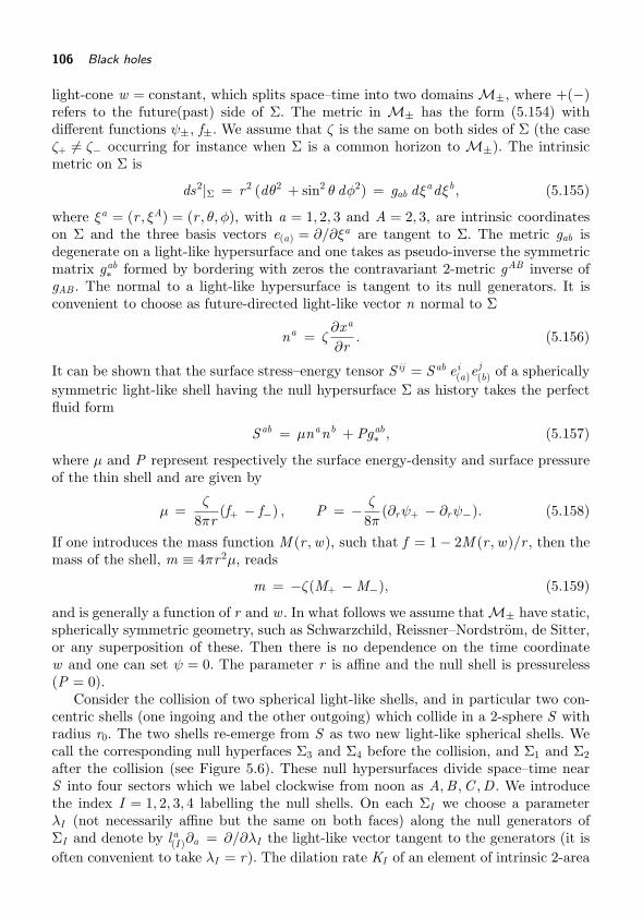
106 Black holes
light-cone w = constant, which splits space–time into two domains M±, where +(−)refers to the future(past) side of Σ. The metric in M± has the form (5.154) withdifferent functions ψ±, f±. We assume that ζ is the same on both sides of Σ (the caseζ+ �= ζ− occurring for instance when Σ is a common horizon to M±). The intrinsicmetric on Σ is
ds2|Σ = r2 (dθ2 + sin2 θ dφ2) = gab dξadξb , (5.155)
where ξa = (r , ξA) = (r , θ, φ), with a = 1, 2, 3 and A = 2, 3, are intrinsic coordinateson Σ and the three basis vectors e(a) = ∂/∂ξa are tangent to Σ. The metric gab isdegenerate on a light-like hypersurface and one takes as pseudo-inverse the symmetricmatrix gab
∗ formed by bordering with zeros the contravariant 2-metric gAB inverse ofgAB . The normal to a light-like hypersurface is tangent to its null generators. It isconvenient to choose as future-directed light-like vector n normal to Σ
na = ζ∂xa
∂r. (5.156)
It can be shown that the surface stress–energy tensor S ij = Sab ei(a)e
j(b) of a spherically
symmetric light-like shell having the null hypersurface Σ as history takes the perfectfluid form
Sab = μnanb + Pgab∗ , (5.157)
where μ and P represent respectively the surface energy-density and surface pressureof the thin shell and are given by
μ =ζ
8πr(f+ − f−) , P = − ζ
8π(∂rψ+ − ∂rψ−). (5.158)
If one introduces the mass function M (r ,w), such that f = 1 − 2M (r ,w)/r , then themass of the shell, m ≡ 4πr 2μ, reads
m = −ζ(M+ − M−), (5.159)
and is generally a function of r and w . In what follows we assume that M± have static,spherically symmetric geometry, such as Schwarzchild, Reissner–Nordstrom, de Sitter,or any superposition of these. Then there is no dependence on the time coordinatew and one can set ψ = 0. The parameter r is affine and the null shell is pressureless(P = 0).
Consider the collision of two spherical light-like shells, and in particular two con-centric shells (one ingoing and the other outgoing) which collide in a 2-sphere S withradius r0. The two shells re-emerge from S as two new light-like spherical shells. Wecall the corresponding null hyperfaces Σ3 and Σ4 before the collision, and Σ1 and Σ2after the collision (see Figure 5.6). These null hypersurfaces divide space–time nearS into four sectors which we label clockwise from noon as A,B ,C ,D . We introducethe index I = 1, 2, 3, 4 labelling the null shells. On each ΣI we choose a parameterλI (not necessarily affine but the same on both faces) along the null generators ofΣI and denote by l a(I )∂a = ∂/∂λI the light-like vector tangent to the generators (it isoften convenient to take λI = r). The dilation rate KI of an element of intrinsic 2-area

Inside the black hole 107
Σ1 Σ2
Σ3Σ4
A
B
C
D r0
Fig. 5.6 Collision of two concentric, spherical, light-like shells Σ3, Σ4 at radius r = r0 resultingin two concentric, spherical, light-like shells Σ1, Σ2.
convected along these generators is equal to KI = 2r−1 l a(I )∂ar , and we form the fourscalar functions
FA =K1K2
l(1) · l(2), FB =
K3K4
l(3) · l(4), FC =
K2K3
l(2) · l(3), FD =
K1K4
l(1) · l(4). (5.160)
Using the property (l(1) · l(2))(l(3) · l(4)) = (l(1) · l(4))(l(2) · l(3)) one sees that, at each pointof the 2-sphere of collision S ,
FAFB = FCFD . (5.161)
Introducing f = gabr,ar,b = grr this relation becomes
fA(r0) fB (r0) = fC (r0) fD (r0). (5.162)
It was first derived by Dray and ’t Hooft (1985) and Redmount (1985) and latergeneralized to cases including rotating black holes by Barrabes et al. (1990). If oneintroduces the local mass functions MA,MB ,MC ,MD , then (5.162) yields a local rela-tion between their values at the collision. For weak fields, to linear order (neglectingquadratic potential energy terms) it expresses conservation of gravitational mass inthe collision. We note that a conservation relation also exists between the masses ofthe shells. Using (5.159) to define the masses mI of the shells, and the sign conventionfor ζ, we find that
m1 = MA − MD , m2 = MC − MA, m3 = MC − MB , m4 = MB − MD , (5.163)
from which immediately follows the conservation relation m1 + m2 = m3 + m4 betweenthe masses of the null shells.
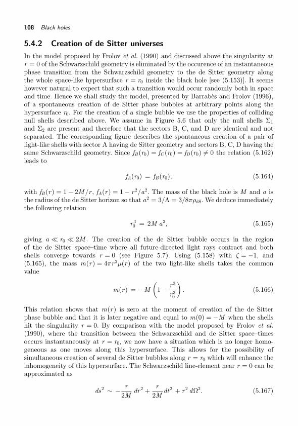
108 Black holes
5.4.2 Creation of de Sitter universes
In the model proposed by Frolov et al. (1990) and discussed above the singularity atr = 0 of the Schwarzschild geometry is eliminated by the occurence of an instantaneousphase transition from the Schwarzschild geometry to the de Sitter geometry alongthe whole space-like hypersurface r = r0 inside the black hole [see (5.153)]. It seemshowever natural to expect that such a transition would occur randomly both in spaceand time. Hence we shall study the model, presented by Barrabes and Frolov (1996),of a spontaneous creation of de Sitter phase bubbles at arbitrary points along thehypersurface r0. For the creation of a single bubble we use the properties of collidingnull shells described above. We assume in Figure 5.6 that only the null shells Σ1and Σ2 are present and therefore that the sectors B, C, and D are identical and notseparated. The corresponding figure describes the spontaneous creation of a pair oflight-like shells with sector A having de Sitter geometry and sectors B, C, D having thesame Schwarzschild geometry. Since fB (r0) = fC (r0) = fD(r0) �= 0 the relation (5.162)leads to
fA(r0) = fB (r0), (5.164)
with fB (r) = 1 − 2M /r , fA(r) = 1 − r 2/a2. The mass of the black hole is M and a isthe radius of the de Sitter horizon so that a2 = 3/Λ = 3/8πρdS. We deduce immediatelythe following relation
r 30 = 2M a2, (5.165)
giving a � r0 � 2M . The creation of the de Sitter bubble occurs in the regionof the de Sitter space–time where all future-directed light rays contract and bothshells converge towards r = 0 (see Figure 5.7). Using (5.158) with ζ = −1, and(5.165), the mass m(r) = 4πr 2μ(r) of the two light-like shells takes the commonvalue
m(r) = −M(
1 − r 3
r 30
). (5.166)
This relation shows that m(r) is zero at the moment of creation of the de Sitterphase bubble and that it is later negative and equal to m(0) = −M when the shellshit the singularity r = 0. By comparison with the model proposed by Frolov et al.(1990), where the transition between the Schwarzschild and de Sitter space–timesoccurs instantaneously at r = r0, we now have a situation which is no longer homo-geneous as one moves along this hypersurface. This allows for the possibility ofsimultaneous creation of several de Sitter bubbles along r = r0 which will enhance theinhomogeneity of this hypersurface. The Schwarzschild line-element near r = 0 can beapproximated as
ds2 ∼ − r2M
dr2 +r
2Mdt2 + r 2 dΩ2. (5.167)
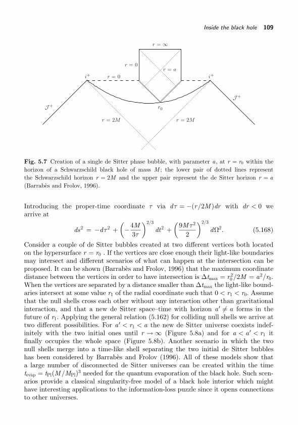
Inside the black hole 109
r = 0
r = 0 i+i+
r0
r = a
r = 2M r = 2M
r = ∞
J+
J+
Fig. 5.7 Creation of a single de Sitter phase bubble, with parameter a, at r = r0 within thehorizon of a Schwarzschild black hole of mass M ; the lower pair of dotted lines representthe Schwarzschild horizon r = 2M and the upper pair represent the de Sitter horizon r = a(Barrabes and Frolov, 1996).
Introducing the proper-time coordinate τ via dτ = −(r/2M )dr with dr < 0 wearrive at
ds2 = −dτ 2 +(−4M
3τ
)2/3
dt2 +(
9M τ 2
2
)2/3
dΩ2. (5.168)
Consider a couple of de Sitter bubbles created at two different vertices both locatedon the hypersurface r = r0 . If the vertices are close enough their light-like boundariesmay intersect and different scenarios of what can happen at the intersection can beproposed. It can be shown (Barrabes and Frolov, 1996) that the maximum coordinatedistance between the vertices in order to have intersection is Δtmax = r 2
0 /2M = a2/r0.When the vertices are separated by a distance smaller than Δtmax the light-like bound-aries intersect at some value r1 of the radial coordinate such that 0 < r1 < r0. Assumethat the null shells cross each other without any interaction other than gravitationalinteraction, and that a new de Sitter space–time with horizon a ′ �= a forms in thefuture of r1. Applying the general relation (5.162) for colliding null shells we arrive attwo different possibilities. For a ′ < r1 < a the new de Sitter universe coexists indef-initely with the two initial ones until r → ∞ (Figure 5.8a) and for a < a ′ < r1 itfinally occupies the whole space (Figure 5.8b). Another scenario in which the twonull shells merge into a time-like shell separating the two initial de Sitter bubbleshas been considered by Barrabes and Frolov (1996). All of these models show thata large number of disconnected de Sitter universes can be created within the timetevap = tPl(M /MPl)3 needed for the quantum evaporation of the black hole. Such scen-arios provide a classical singularity-free model of a black hole interior which mighthave interesting applications to the information-loss puzzle since it opens connectionsto other universes.

110 Black holes
r = 0 r = 0
r0r0
r = a
r = ∞
a
a
M
(a)
r = 0 r = 0
r0r0
r = ∞
a a
r = a
M
(b)
Fig. 5.8 Creation of a pair of de Sitter phase bubbles with parameter a at r = r0 followed by theintersection of their boundaries at M(r = r1) and the subsequent production of a new de Sitteruniverse with parameter a ′; case (a) corresponds to a′ < r1 < a and case (b) to a < a ′ < r1
(Barrabes and Frolov, 1996).
5.5 Metric fluctuations and Hawking radiation
In his original derivation of black hole radiance Hawking (1975) considered thepropagation of a linear quantized field in a classical background geometry [see alsoBirrel and Davies (1982) and Carroll (2004)]. The mean value of the energy–momentumtensor is taken as the source of the gravitational field which is itself treated classic-ally. The validity of this semiclassical approach has been questioned, in particular thecontroversial role of arbitrarily large (‘transplanckian’) frequencies of vacuum fluctu-ation (’t Hooft 1985, 1996, Brout et al. 1995) and the impact of gravitational backreaction due the emission of quanta. Zero-point fluctuations of quantum fields inducefluctuations of the metric. We study in this section how the fluctuations of the blackhole geometry affect the properties of Hawking radiation (Barrabes et al., 1999). Todescribe these fluctuations quantum mechanically and to determine their effects onHawking radiation requires full quantum gravity which is technically a very complic-ated problem. The modifications of Hawking radiation due to the metric fluctuationswill be extracted within a simpler framework in which these fluctuations are treatedclassically. Furthermore only spherically symmetric fluctuations will be considered andthe scattering by the gravitational potential barrier which occurs in the 4-dimensionald’Alembertian will be neglected.
We use a model proposed by York (1983) in which the fluctuating geometry nearthe horizon of the black hole is represented by a Vaidya metric with a fluctuatingmass. Using an advanced time coordinate the Vaidya line-element reads
ds2 = −(
1 − 2m(v)r
)dv 2 + 2dv dr + r 2 dΩ2, (5.169)
with here
m(v) = M [1 + μ(v)]θ(v), (5.170)

Metric fluctuations and Hawking radiation 111
μ(v) = μ0 sin(ωv)θ(v). (5.171)
The mass of the black hole fluctuates with frequency ω and the dimensionless amp-litude μ0 is assumed to be small (μ0 � 1) for a black hole with mass M much largerthan the Planck mass. The Heaviside step function θ(v) in (5.170) indicates that theformation of the black hole results from the collapse of a massive null shell with massM . The origin v = 0 of the advanced-time coordinate is taken to correspond to thecollapse of the shell (see Figure 5.9). Hence for v < 0 the space–time geometry is flatwhile it is of Vaidya type when v > 0.
r = 0
r = 0
i +
A
B
P
H
Qu
J+
J−
v = 0
VH
V0(u)
Fig. 5.9 Conformal diagram of a black hole formed by the collapse of a spherical null shell; thedouble line v = 0 is the history of the collapsing null shell. The solid dark line PABQ represents alight ray leaving J− at advanced time v = V0(u) and reaching J + at retarded time u (Barrabeset al., 1999).

112 Black holes
The energy–momentum tensor associated with the metric (5.169) is given by
Tab =la lb4πr 2 [M δ(v) + Mμ(v) θ(v)] , (5.172)
where la = −v,a is a future-directed null vector field tangent to ingoing radial nullrays. The first term in Tab corresponds to the collapsing null shell whose space–timehistory is the null hypersurface v = 0 and the second term is the source of the Vaidyametric. We use the geometric optics approximation to obtain the solution of the waveequation and to study the propagation of radial null rays in the fluctuating geometry(5.169). Ingoing radial null rays are given by v = constant, while outgoing null raysobey the equation (
1 − 2m(v)r
)dv = dr . (5.173)
In order to solve this equation we use a perturbation method and write
r(v) = R(v) + ρ(v) + σ(v) + · · · . (5.174)
Here R(v) is the solution in the absence of fluctuations (μ0 = 0) while ρ(v) and σ(v)are first- and second-order terms, respectively, in the perturbation parameter μ0. Wefind from (5.173) when v > 0 that
2dRdv
= 1 − 2MR
, (5.175)
2dρ
dv− 2M
R2 ρ = −2MR
μ, (5.176)
2dσ
dv− 2M
R2 σ =2MR
[ρμ
R− ρ2
R2
]. (5.177)
We begin by looking for the perturbed position, rH = RH + ρH + σH + · · · , of theevent horizon. From the zeroth-order equation R is constant and equal to RH = 2M .Introduction of this value into (5.176) and (5.177) and solving these equations leadsto the following:
ρH = 2Mμ0
[Ω cos(ωv) + sin(ωv)
1 + Ω2
], (5.178)
σH = 2Mμ20
[2Ω2(2 − Ω2) cos(2ωv) + Ω(1 − 5Ω2) sin(2ωv)
2(1 + Ω2)2(1 + 4Ω2)
]. (5.179)
We have introduced here the dimensionless frequency Ω = ω/κ where κ = (4M )−1
is the surface gravity of the unperturbed black hole with mass M . The resultingexpression of rH shows that the position of the event horizon of the perturbed blackhole fluctuates. It follows that the surface area A(v) = 4πr2
H of the event horizon andthe surface gravity κ = m(v)/r 2
H also fluctuate and have mean values equal to
A ∼ 16πM 2[1 +
μ20
2(1 + Ω2)
], (5.180)

Metric fluctuations and Hawking radiation 113
and
κ ∼ κ
[1 +
μ20
2(1 + Ω2)
], (5.181)
respectively. Computation of the modified Hawking flux of radiation will later showthat κ is identical to the renormalized surface gravity. The mean value of the Hawkingtemperature is TH = κ/2π (in units for which the Boltzman constant is unity) and thechanges of area δA = A − A and of temperature δTH = TH − TH obey the relation
δAA =
δTH
TH. (5.182)
This induces a modification of the entropy of the black hole. Its mean value satisfiesdS = dE/TH where E = m(v) = M and it is equal to
S =A4
(1 − μ2
0
2(1 + Ω2)
), (5.183)
instead of the usual relation S = A/4.We start by studying Hawking radiation in the absence of metric fluctuations (so
that μ0 = 0) and considering an outgoing null ray which reaches future null infinity J +
at a given value u of retarded time. Tracing back in time this null ray one arrives at thetrajectory PABQ on Figure 5.9. Such a ray starts from past null infinity J−, convergesradially and diverges again after bouncing off at (r = 0). On its way towards J + itcrosses the null shell where v = 0. Our aim is to obtain the relation V0(u) between thevalue of the advanced time at the departure of the ray from J− and the value of theretarded time at its arrival at J +. The future of a null ray leaving J − has a differentdestination depending upon the value of the advanced time at its departure. Looking atFigure 5.9 and considering all possibilities for ingoing null rays leaving J− at differentvalues of v one sees that: (i) for v > 0 the ray directly hits the singularity r = 0; (ii)for v < VH the ray reaches J + after reflection at r = 0; and (iii) for VH < v < 0 theray propagates in the trapped region until reaching the singularity after reflection atr = 0. Only case (ii) is relevant for the study of Hawking radiation.
We first derive the relation V0(u) in the absence of fluctuation (μ0 = 0). In theflat space–time domain (v < 0) we have the usual relation v − u = 2r and in theSchwarzschild domain (v > 0) this relation becomes v − u = 2[r − 2M + 2M ln{(r −2M )/2M }] [see (5.5) and (5.6)]. In both domains v (u) is constant along an ingoing(outgoing) radial null ray. Calling V0 the initial value of advanced time at departurefrom J −, and R0 the value of the radial coordinate when the ray crosses the shell atv = 0, it can be shown that
V0 = −2R0 and − u = 2[R0 − 2M + 2M ln
(R0
2M− 1
)]. (5.184)
The first relation in (5.184) is obtained when v < 0 and the second when v > 0. Sincethe radial coordinate is continuous across the singular null hypersurface (v = 0) theserelations combine to give the required expression for V0(u).
In the presence of metric fluctuations (μ0 �= 0) the part of the trajectory in thedomain v > 0 is modified and to the same retarded time u at arrival at J + will

114 Black holes
correspond a new value V (u) of advanced time at departure from J −. The firstequation in (5.184) is now replaced by
V (u) = −2[R0(u) + ρ0(u) + σ0(u)], (5.185)
where the subscript zero still refers to the interesection of the ray with the hypersur-face v = 0. The first- and second-order terms ρ and σ of (5.174) are solutions of theequations (5.176) and (5.177). These equations can be rewritten in the common form
dfdv
− Mf 2 = F , (5.186)
with
f = ρ , F = −MR
, (5.187)
for the first-order perturbation and
f = σ , F =MR2 μρ − M
R3 ρ2, (5.188)
for the second-order perturbation. It is convenient to use (5.175) in order to replacethe variable v by the dimensionless variable x = (R − 2M )/2M and to introduce thedimensionless quantities
u = κu , V = κV , ρ =ρ
2M, σ =
σ
2M. (5.189)
We then find that
ρ(x ) =x
1 + x
∫ ∞
x
dξ
ξ2 (1 + ξ)μ(ξ), (5.190)
σ(x ) = − x1 + x
∫ ∞
x
dξ
ξ2 ρ(ξ)[μ(ξ) − ρ(ξ)
1 + ξ
], (5.191)
where μ(ξ) = μ0 sin[Ω(ξ + ln ξ + u)]. In these equations the constant of integration hasbeen chosen in such a way that the perturbed ray arrives at J + at the same retardedtime u as the unperturbed one. Introducing these results into (5.185) results in
V (u) = −[1 + x0 + ρ(x0) + σ(x0)], (5.192)
where x0 = (R0 − 2M )/2M satisfies
u = −x0 + ln x0. (5.193)
We are interested in the rays propagating near the horizon and arriving at J + at latetime u � 1. Solving (5.193) by iteration gives
x0 = e−u (1 − e−u) + O(e−3u), (5.194)
showing that x0 is a very small quantity. After some lengthy calculations it can beshown that V (u) takes the following form [cf. equations (5.2)–(5.5) of Barrabes et al.(1999)]
V (u) = −e−u [1 + A1 sin(Ωu + ϕ1) + A2 sin(2Ωu + ϕ2) + Cu] , (5.195)

Metric fluctuations and Hawking radiation 115
where A1,A2 and the phases ϕ1, ϕ2 are functions of the dimensionless frequency Ω =ω/κ and C is given by
C = − μ20
2(1 + Ω2). (5.196)
We do not need A2 or ϕ2 for our final results. For A1 and ϕ1 we have
A1 = μ0q(Ω)
(1 + Ω2)1/2 + 2μ20q(Ω)(Ω2 − 1)Ω(1 + Ω2)3/2 , (5.197)
ϕ1 = −ϕΓ(Ω) + arctan Ω, (5.198)
where ϕΓ(Ω) is a real function which, for large values of Ω, behaves as ϕΓ ∼ Ω, and
q(Ω) =√
2π√Ω(e2πΩ − 1)
. (5.199)
Finally we study the energy flux and the asymptotic spectrum of Hawking radi-ation. To this end we calculate the contribution of the s-mode of a quantum scalarmassless field to Hawking radiation. Neglecting the scattering by the gravitationalpotential barrier amounts to using a 2-dimensional approximation in which ingoingand outgoing modes decouple completely. Assuming that the field is in its vacuumstate before the formation of the black hole, we use the following relation which givesthe mean energy flux of Hawking radiation at J +:
dEdu
≡ 4πr 2 〈Tuu〉ren =κ2
12π
(dVdu
)1/2d2
du2
⎡⎣(dV
du
)−1/2⎤⎦ . (5.200)
Introducing (5.195) into this equation produces an expression which can be writtenas the sum of a permanent part and a fluctuating part. Only the permament part willcontribute to the total energy received at J +. Direct calculation yields(
dEdu
)perm
=κ2
48π
[1 +
12μ2
0 Ω2 q2(Ω) − 2C]
, (5.201)
with C given by (5.196). This latter term, which gave a linear contribution in (5.195),does not contribute to the fluctuating part of dE/du. Since μ0 � 1 it can be absorbedinto eu and removed from (5.195). Such a transformation corresponds to the renor-malization of the surface gravity, κ → κr = κ(1 − C ). We note that it is identical tothe mean value κ introduced earlier in (5.181). Hence the permanent part of the meanenergy flux at J + can be rewritten as(
dEdu
)perm
=κ2
r
48π
[1 + μ2
0πΩ
e2πΩ − 1
]. (5.202)
The modifications of the energy flux, which are due to the fluctuations of the met-ric, manifest themselves in the renormalized surface gravity [see (5.196)] and in theadditional term μ2
0 πΩ(/(e2πΩ − 1). Both modifications are of second order in μ0 and

116 Black holes
decrease when the frequency of the fluctations increases. In the absence of fluctuationsthe usual expression of (dE/du)0 = κ2/(48π) holds.
Still using the 2-dimensional aproximation, and neglecting the effect of the grav-itational barrier, we can extract the asymptotic spectrum of Hawking radiation fromthe properties of the Bogoliubov coefficients (Birrel and Davies 1982, Carroll 2004,Brout et al. 1995). These coefficients are given by the overlap of the initial (ingoing)modes which are specified at J− and the final (outgoing) modes specified at J +.Since s-modes satisfy the 2-dimensional equation ∂u∂vφ = 0 they can be decomposedin terms of plane waves as
φν(v) =e−iνv√
4πν, φλ(u) =
e−iλu√
4πλ, (5.203)
where ν is the energy measured at J− for the in-modes, and λ is the energy measuredat J + for the out-modes. The reflection condition at r = 0 implies that the scatteredin-modes are given by φν(V (u)). Then the Bogoliubov coefficients are given by
αν,λ =∫
du φ∗ν(V (u)) i
←→∂u φλ(u) =
∫du
eiν V (u)√
4π ν
e−iλ u√
πλ−1, (5.204)
βν,λ =∫
du φν(V (u)) i←→∂u φλ(u) =
∫du
e−iν V (u)√
4π ν
e−iλ u√
πλ−1. (5.205)
In the unperturbed geometry one sees from (5.192) and (5.193) that for largeu, κV0(u) = −1 − e−κ u approximately. Extending the domain of validity of theasymptotic behaviour of V0(u) for all u, one finds that
αν,λ = B(ν, λ)eπλ/κe−ν/κ
√2πκν
, βν,λ = B(ν, λ)eπλ/κ
√2πκν
, (5.206)
where the function B(ν, λ) is given by
B(ν, λ) = Γ(
iλκ
) √λ
2πκ
(ν
κ
)−iλ/κ
e−πλ/2κ, (5.207)
and Γ(z ) is the gamma function. The mean number of quanta reaching J + per unitretarded time is derived from the general expression
< nλ >=∫ N dν |βν,λ|2∫ N dν/κν
. (5.208)
The time average here is obtained by integrating over ν up to the cut-off frequency Nand then dividing the resulting expression by the denominator as indicated.
Without fluctuations of the metric the mean number of quanta reaching J + takesthe form
< nλ >0 =12π
1e2πλ/κ − 1
. (5.209)
This is a Planck distribution with temperature T = κ/2π = (8πM )−1. In the pres-ence of fluctuations one needs to use the perturbed expression (5.195) for V (u).

Metric fluctuations and Hawking radiation 117
This leads to a modification of the mean rate of quanta reaching J + which is nowequal to
〈nλ〉 =12π
1e2πλ/κr − 1
−(
A1
2κr
)2 2λ
e2πλ/κr − 1,
+(
A1
2κr
)2 [λ − ω
e2π(λ−ω)/κr − 1+
λ + ω
e2π(λ+ω)/κr − 1
], (5.210)
where A1 is given by (5.197). The modifications of the asymptotic spectrum of Hawkingradiation appear in the renormalization of surface gravity and in the existence of threeadditional terms. Among them the two last terms in (5.210) contain Bose thermalfactors showing that ±ω plays the role of a chemical potential which facilitates leakageof energy and is reminiscent of superradiance.

6Higher dimensional black holes
Higher dimensional space–times, with dimensions D = 4 + k with k > 0, are a commoningredient in most theories attempting to unify gravity with the other forces of nature.This idea, which originated a long time ago with the work of Kaluza (1921) andKlein (1926), has received a new impetus from later developments in field theory and,in particular, string theories. The k extra dimensions have so far eluded detection,the conventional explanation being that they are compactified within radii of theorder of the Planck length lPl ∼ 10−33cm. This corresponds to energies of the order ofEPl = 1019 GeV which are well out of reach compared to energies currently available.Some recent models consider larger dimensions [as large as a millimetre (Antoniadiset al., 1998)] and even infinite extra dimensions (Randall and Sundrum, 1999). Theyhave received a lot of attention because they offer a way to lower energy from thePlanck scale to the weak scale (of TeV order) and to provide an explanation for thelarge disparity between these two scales (the so-called hierarchy problem). They alsoraise the prospect of experimental verification and, in particular, the production ofmini black holes at future colliders. In the so-called brane-world models the standardfields are confined to a 4-dimensional time-like hypersurface (the brane) embedded ina higher dimensional space–time (the bulk) where only gravity can propagate. Blackholes on the other hand can be either attached to the brane or move in the bulk.
Let us assume that the k extra dimensions have radius of order l , and call respect-ively MPl,D and GD the Planck mass and the gravitational coupling constant for aD-dimensional space–time. In the ordinary case D = 4 the D index is omitted and wewrite simply MPl and G for these quantities. At distances r � l much smaller than theradii of the extra dimensions the gravitational force has the usual expression derivedfrom Gauss’ law:
F = GDm1m2
r 2+k . (6.1)
On the other hand, when r � l the extra dimensions can be ignored and thegravitational force can be approximated as
F ∼ GDm1m2
l k r 2 . (6.2)
Hence the corresponding effective 4-dimensional gravitational constant G is such thatG ∼ GD l−k , in units for which � = c = 1. From the definition of the Planck mass inarbitrary dimensions one has GDM D−2
Pl,D = 1 and therefore
M k+2Pl,D ∼ M 2
Pl l−k . (6.3)

Brief outline of D-dimensional black holes 119
This relation shows that increasing the size of the extra dimensions lowers the Planckscale which can eventually be made of the order of the electroweak scale MEW ∼ TeV(for example with k = 2 and l ∼ 100 μm−1 mm).
Another interesting consequence of large extra dimensions is the possible pro-duction of mini black holes at an energy scale which is accessible to high-energyexperiments and exists in cosmic rays (Eardley and Giddings 2002, Rychkov 2004,Yoshino and Rychkov 2005, Cardoso et al. 2005, Horowitz 2012). Describing scatter-ing processes of elementary particles leading to the production of black holes requiresa full theory of quantum gravity. Since in these processes the centre-of-mass energyis much larger than the Planck mass a semiclassical approach can be followed. Itis thus important to extend to higher dimensions properties of black holes whichare already known in four dimensions. In this chapter, after a brief description ofD > 4-dimensional black holes, we generalize to arbitrary dimensions the geometricalinequalities, already presented in Chapter 5, which give conditions for the formation ofa trapped surface. This has application to the formation of apparent horizons (and thusof a black hole) in the collision of high-energy particles, as in the work of Yoshino andNambu (2002). Also since scattering by ultra-relativistic spinning particles requires aknowledge of their gravitational fields the metric of a D-dimensional Kerr black holeboosted to the speed of light will be derived. This has been used to propose a modelof the gravitational field of a spinning radiation beam pulse (a gyraton) in higherdimensions (Frolov and Fursaev 2005, Frolov, Israel and Zelnikov 2005).
6.1 Brief outline of D-dimensional black holes
Black holes are characterized by the presence of an event horizon. In a 4-dimensionalstationary space–time a theorem of Hawking states that the surface topology of theevent horizon has to be a 2-sphere, and furthermore uniqueness theorems for blackhole solutions have been demonstrated. These properties are lost in dimensions largerthan four. There exist solutions for which the event horizon has the topology of a(D − 2)-sphere (SD−2) and one still speaks of black holes. There also exist solutionswith different topology, such as for example black rings where the event horizon hasthe topology S 1 × SD−3 (Emparan and Reall 2002, Emparan and Myers 2003, 2008).
The higher dimensional analogue of the Schwarzschild 4-D solution of the vacuumEinstein equations was obtained a long time ago by Tangherlini (1963). Its line-elementhas the form
ds2 = −f (r) dt2 +1
f (r)dr 2 + r 2 dΩ2
D−2, (6.4)
where r is the radial coordinate, and dΩ2D−2 is the line-element of the unit (D − 2)-
sphere (dΩ2n+1 = dθ2
n+1 + sin2 θn dΩ2n for n ≥ 1). The function f (r) is given by
f (r) = 1 − 16πGD M(D − 2)sD−2 rD−3 . (6.5)

120 Higher dimensional black holes
Here M is the mass of the black hole and sn is the area of the unit sphere Sn . Thus
sD−2 =2π(D−1)/2
Γ(D−12 )
, (6.6)
with the gamma function appearing in the denominator. The Tangherlini solutionhas the same causal structure as the Schwarzschild solution. It has an event horizoncorresponding to the value r = rH of the radial coordinate such that
rH =(
16πGDM(D − 2) sD−2
)1/(D−3)
. (6.7)
Note that this relation shows that GDM ∼ (length)D−3.The metric of a D-dimensional rotating black hole has been obtained by Myers and
Perry (1986). While in four dimensions Kerr black holes have only two paramaters,the mass M and the angular momemtum parameter a, in D > 4 dimensions they arecharacterized by the mass M and l angular momentum parameters where l is given by
l =[D − 1
2
]. (6.8)
The notation [N ] indicates the integer part of N . Thus l = (D − 1)/2 when D is oddand l = (D − 2)/2 when D is even. The number l of angular momentum parametersis related to the existence of [(D − 1)/2] Casimirs of the group SO(D − 1) of spatialrotations. It represents here the number of independent 2-planes of rotation. Thel angular momentum parameters will be denoted by ai with i = 1, 2, . . . , l and theangular momentum in the i -th plane of rotation is
Ji =2M
D − 2ai . (6.9)
The Myers–Perry metric admits the (l + 1) Killing vectors ξ(t) = ∂t and ξ(i) = ∂φi
with i = 1, 2, . . . , l . It is the most general metric describing the field of a D-dimensionalrotating black hole and is most easily written in the Kerr-Schild form:
gab = ηab + H kakb , (6.10)
where ka is a null vector and H a function of the coordinates xa , with a = 1, 2, . . . ,Dand xD = t being the time cordinate. Also ηab is the D-dimensional Minkowskimetric, ka = gabkb = ηabkb and gab = ηab − H kakb . For the spatial coordinates it isconvenient to replace the set (x 1, . . . , xD−1) by either the l = (D − 1)/2 pairs ofcoordinates (x i , yi) with i = 1, 2, . . . , l when D is odd or, when D is even, by the set(x i , yi , xD−1 ≡ z ) with now l = (D − 2)/2. For odd values of D we have l = (D − 1)/2and we define
F = 1 −l∑
i=1
a2i((x i )2 + (yi )2
)(r 2 + a2
i )2 , (6.11)
Π =l∏
i=1
(r2 + a2i ), (6.12)
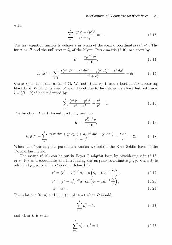
Brief outline of D-dimensional black holes 121
withl∑
i=1
(x i )2 + (yi )2
r 2 + a2i
= 1. (6.13)
The last equation implicitly defines r in terms of the spatial coordinates (x i , yi ). Thefunction H and the null vector ka of the Myers–Perry metric (6.10) are given by
H =rD−3H r 2
F Π, (6.14)
ka dxa =l∑
i=1
r(x i dx i + yi dyi ) + ai (x i dyi − yi dx i)r 2 + a2
i− dt , (6.15)
where rH is the same as in (6.7). We note that rH is not a horizon for a rotatingblack hole. When D is even F and Π continue to be defined as above but with nowl = (D − 2)/2 and r defined by
l∑i=1
(x i)2 + (yi)2
r 2 + a2i
+z 2
r 2 = 1. (6.16)
The function H and the null vector ka are now
H =rD−3H rF Π
, (6.17)
ka dxa =l∑
i=l
r(x i dx i + yi dyi ) + ai (x i dyi − yi dx i )r 2 + a2
i+
z dzr
− dt . (6.18)
When all of the angular parameters vanish we obtain the Kerr–Schild form of theTangherlini metric.
The metric (6.10) can be put in Boyer–Lindquist form by considering r in (6.13)or (6.16) as a coordinate and introducing the angular coordinates μi , φi when D isodd, and μi , φi , α when D is even, defined by
x i = (r 2 + a2i )1/2μi cos
(φi − tan−1 ai
r
), (6.19)
yi = (r 2 + a2i )1/2μi sin
(φi − tan−1 ai
r
), (6.20)
z = α r . (6.21)
The relations (6.13) and (6.16) imply that when D is odd,l∑
i=1
μ2i = 1, (6.22)
and when D is even,l∑
i=1
μ2i + α2 = 1. (6.23)
122 Higher dimensional black holes
Following further coordinate transformations t → t and φi → φi , to eliminate some ofthe off-diagonal components of the metric, the line-element when D is odd becomes
ds2 =ΠF
Π − rD−3H r 2
dr 2 +l∑
i=1
(r 2 + a2i ) (dμ2
i + μ2i d φ2
i )
+rD−3H r 2
ΠF(d t + ai μ2
i d φi )2 − d t2, (6.24)
and when D is even becomes
ds2 =ΠF
Π − rD−3H r
dr 2 +l∑
i=1
(r 2 + a2i ) (dμ2
i + μ2i d φ2
i )
+ r2 dα2 +rD−3H rΠF
(d t + ai μ2i d φi )2 − d t2, (6.25)
with F and Π given by (6.11) and (6.12). Using these forms of the line-element forlarge values of r the interpretation of M , introduced in (6.5), and of Ji , introducedin (6.9), as, respectively, the mass and the angular momentum in the i -th plane ofrotation is confirmed.
The horizons of a rotating D-dimensional black hole are given by the solutions ofgrr = (grr )−1 = 0. From (6.24) and (6.25) these equations become
Π − rD−3H r 2 = 0, (6.26)
when D is odd and
Π − rD−3H r = 0, (6.27)
when D is even. The singularities, horizons, and their topology have been discussedby Myers and Perry (1986). Other properties concerning the existence of Killing–Yanotensors and symmetric Killing tensors generating symmetries which are analogous tothose of the 4-dimensional Kerr black hole are described by Frolov and Sojkovic (2003),Frolov (2003), Frolov and Kubiznak (2007), and Frolov and Zelnikov (2011).
6.2 Gibbons–Penrose isoperimetric inequality and the hoopconjecture in D dimensions
In this section we generalize the results of the previous chapter to space–times withdimension D > 4. As in Chapter 5 we use the Penrose model of a convex thin shellcollapsing in a vacuum from infinity with the speed of light. It is easy to see that thefollowing equation still holds:
K = 16πGD μ, (6.28)
where K is the extrinsic curvature of the (D − 2)-surface of the shell and μ is its surfaceenergy density. The gravitational constant GD now appears in (6.28) as this relation

Gibbons–Penrose isoperimetric inequality and the hoop conjecture in D dimensions 123
is obtained from the D-dimensional analogue of Raychaudhuri’s equation (5.36). Thetotal mean curvature Q of the shell is defined by
(D − 2)Q =∫
KdS . (6.29)
With M =∫
μdS the total conserved mass (identical with the ADM mass and Bondiadvanced mass) of the shell, we find from (6.28) and (6.29) that
(D − 2)Q = 16πGD M . (6.30)
In arbitrary dimensions the Minkowski inequality (Minkowski, 1903) [see also Buragoand Zalgaller (1988), p. 212] states that: for any closed convex m-dimensional surfaceimmersed in Rn , with 2 ≤ m < n, its area Am satisfies
sm (Am)m−1 ≤ Qm , (6.31)
where Q is the total mean curvature and sm is the area of the unit m-sphere [see(6.6)]. If (6.31) is applied to the imploding shell we obtain, since m = D − 2 and using(6.30), the D-dimensional form of the Gibbons–Penrose isoperimetric inequality
sD−2 (AD−2)D−3 ≤(
16πGDMD − 2
)D−2
. (6.32)
According to this a marginally trapped surface, and therefore an apparent horizon,forms during the collapse of the shell provided its mass M is concentrated withina sufficiently compact domain whose boundary has an area satisfying (6.32). TheGibbons–Penrose inequality of general relativity, A2 ≤ 4 (2GM )2, is recovered byputting D = 4 in (6.32). Introducing the Schwarzschild radius
rH =(
16πGDM(D − 2) sD−2
)1/(D−3)
, (6.33)
into (6.32) yields another familiar form of the Gibbons–Penrose inequality
(AD−2)D−3 ≤ sD−2 rD−2H . (6.34)
We now consider the hoop conjecture in the present context. In order to generalizethe inequalities (5.41) to higher dimensions we first need to obtain the generalizedform of the geometrical inequalities (5.40). The following proposition has been estab-lished by Barrabes et al. (2004): Let D be a convex domain of Rn and Q the totalmean curvature of the boundary ∂D of D. Let ωn−2 be the maximum area of theboundary of its orthogonal hyperplane projections, and Ωn−2 the maximum area of(n − 2)-dimensional sections of ∂D by hyperplanes. Then the total mean curvature Qsatisfies the following inequalities
sn
2sn−2Ωn−2 ≤ Q ≤ sn−1
sn−2ωn−2. (6.35)
The derivation of this proposition is based upon two geometrical results. The first isthe Cauchy formula which states that between the area An−1(∂D) of the boundary
124 Higher dimensional black holes
∂D of a convex domain D ∈ Rn and the mean volume Vn−1(pξ(D)) of the orthogonalplane projections of D in an arbitrary direction there exists the relation
An−1(∂D) =1
bn−1
∫ξ∈Sn−1
Vn−1(pξ(D)) dS . (6.36)
In this expression Sn−1 is the unit (n − 1)-sphere, bn the volume of the unit n-ballwith sn−1 = n bn , ξ is a unit vector, and pξ indicates the projection in the directionof ξ onto a hyperplane orthogonal to ξ. The second geometrical result applies to anycompact q-dimensional domain D ∈ Rp+q , with p ≥ 2, and states that its area Aq(D)obeys the equality
Aq(D) =sp
sp−1sp+q
∫ξ∈Sp+q−1
An−2(pξ(D))dξ, (6.37)
where ξ and pξ have the same significance as in the Cauchy formula (6.36). The Cauchyformula is then used to obtain the lower bound of (6.35) and the upper bound is aconsequence of (6.37). If we now introduce into (6.35) the relation (6.30) between themass M of the shell and the total mean curvature Q we find, since n = D − 1, that
sD−1
2sD−3ΩD−3 ≤ 16GD
D − 2M ≤ sD−2
sD−3ωD−3. (6.38)
The formulae
sn
sn−2=
2π
n − 1and
sn−1
sn−2=
√π
Γ(n−1
2
)Γ( n
2
) ωD−3, (6.39)
can be used to rewrite (6.38) as
π
D − 2ΩD−3 ≤ 16GD
D − 2M ≤
√π
Γ(D−2
2
)Γ(D−1
2
)ωD−3. (6.40)
The inequalities (6.40) specialize to the inequalities (5.41) in the particular caseof D = 4. Since we have the dimensional relation GDM ∼ ΩD−3 ∼ ωD−3 ∼(length)D−3, what was referred to as a hoop in general relativity becomes a (D − 3)-dimensional closed strip in a space–time with D dimensions. In the brane-world modelsonly one of the D − 3 dimensions of the strip belongs to the brane; the D − 4 remainingdimensions are in the bulk.
6.3 Light-like boost of higher dimensional black holes
Working with the Riemann curvature tensor, which is gauge invariant and unambigu-ously represents the gravitational field, is a mathematically sound approach to describea Lorentz boosted gravitational field. Such an approach was adopted to obtain thegravitational field of an isolated gravitating body boosted to the velocity of light andwas illustrated with many examples (Barrabes and Hogan 2003b) and used to derivescattering properties of high-speed sources (see Chapter 5). Since this method howeverrequires lengthy calculations in four dimensions, only the weak field approximation will

Light-like boost of higher dimensional black holes 125
be considered for space–times with arbitrarily large dimensions. The validity of thisapproximation will be checked against the case of the D = 4 Kerr black hole for whichthe exact solution is known.
To begin with consider a black hole with mass M and angular momentum para-meter a rotating around the z -axis of the Cartesian coordinates (x , y , z ). The Lorentzboost can be implemented in an arbitrary direction (Barrabes and Hogan, 2004a) butfor simplicity we only consider here the two cases corresponding to a longitudinal boostin the z -direction or to a transverse boost in (say) the x -direction. In both cases themass of the black hole is rescaled as M = p γ−1 where γ is the Lorentz factor. Withsuch a rescaling the energy p stays finite since M → 0 when γ → ∞. The angularmomentum parameter is rescaled differently according to the direction of the boost.A justification of this can be given by boosting a gravitating body with multipolemoments and is described by Barrabes and Hogan (2003b) in the 4-dimensional case.For a transverse boost (in the direction of the x -axis) the angular momentum para-meter a is not rescaled. Then since M → 0 the angular momentum J = Ma vanishesin the limit γ → ∞ and we obtain the boosted Kerr space–time with line-element
ds2 = −du dv + dy2 + dz 2 − 4p δ(u) ln[(y − a)2 + z 2] du2, (6.41)
with u = t − x , and v = t + x . It is clear from this that although J → 0 the influenceof rotation is still present in this line-element through the appearance of the parametera. The line-element (6.41) describes the space–time model of the gravitational field ofa plane-fronted impulsive gravitational wave whose history is the null hyperplane withequation u = 0. The null generator of this hypersurface corresponding to y = a, z = 0is a line singularity which is a remnant of the Kerr black hole. In comparison withthe metric of a boosted Schwarzschild black hole [see (6.42)] the rotation producesa shift in this line singularity in the y-direction. This effect, known for a long time,has been checked by considering the deflection of highly relativistic particles in theKerr gravitational field (Barrabes and Hogan, 2003b). For a longitudinal light-likeboost (in the direction of the z -axis) the angular momentum parameter is rescaled asa = aγ, with a finite. Hence a → 0 when γ → ∞ and the boosted Kerr space–timehas line-element in this case given by
ds2 = −du dv + dy2 + dz 2 − 4p δ(u) ln(x 2 + y2) du2, (6.42)
with u = t − z and v = t + z . This time the effect of rotation completely disappearsand the boosted line-element is the Aichelburg–Sexl (1971) line-element, which isthe line-element of the boosted Schwarzschild space–time. This line-element againdescribes the space–time model of the gravitational field of an impulsive plane gravit-ational wave with space–time history u = 0 and has a singularity on the null geodesicgenerator y = z = 0 of the null hypersurface u = 0.
We now compare these exact results with the expression for the boosted Kerrline-element which is obtained by imposing from the very beginning the weak fieldapproximation (i.e. M and a small). We thus start with the following linearized formof the Kerr line-element
ds2 = ηabd x ad x b +2Mr
(d t2 + dx 2 + dy2 + dz 2 ) +4Mar3 (x d y − yd x )d t , (6.43)

126 Higher dimensional black holes
where x a = (x , y , z , t), and r2 = x 2 + y2 + z 2. As before the bar refers to a quantitybefore making the Lorentz boost, and the same unbarred quantity corresponds to itsboosted value after taking the limit γ → ∞. The following two formulae will now beused and will also later be useful for dimensions D > 4:
limγ→∞
γ√γ2u2 + ρ2
= −2 ln |ρ|δ(u) +1|u| , (6.44)
and, for m > 1,
limγ→∞
γ
(γ2u2 + ρ2)m/2 =√
πΓ(m−1
2 )Γ(m
2 )δ(u)ρm−1 . (6.45)
Here Γ(x ) is the gamma function satisfying the relations Γ(x + 1) = x Γ(x ) for x > 0,Γ(1) = Γ(0) = 1 and Γ(1/2) =
√π.
In the case of a longitudinal boost (i.e. for t = γ(t − vz ), z = γ(z − vt), x = x ,y = y) both M and a are rescaled. When γ → ∞ we have dz ∼ −γdu and d t ∼ γduand the line-element (6.43) becomes
ds2 = ηαβdxαdx β +4p|u|du
2 − 4p ln(x 2 + y2) δ(u) du2, (6.46)
with u = t − z . A coordinate transformation then brings this line-element into theform (6.42). As noted earlier the rescaling of a in this case wipes out the effectof rotation. For a transverse boost along the x -axis (i.e. for t = γ(t − vx ), x =γ(x − vt), y = y , z = z ) and in the limit γ → ∞ we have dx ∼ −γdu and d t ∼ γdu,with u = t − x . In this case only the mass M is rescaled and not a and the boostedline-element (6.43) is given by
ds2 = −dudv + dy2 + dz 2 +4p|u|du
2 − 8p δ(u)(
ln ρ − ayρ2
)du2, (6.47)
with ρ =√
y2 + z 2, u = t − x , and v = t + x . It is easy to check that (6.47) is identicalto the linearized form of (6.41) for small M and small a.
We now apply the weak field approximation to higher dimensional (D > 4) blackholes, and consider rotating black holes, the non-rotating solution being simplyobtained by equating to zero all the angular momentum parameters. The line-elementis given by (6.10) with the additional relations (6.11)–(6.16). When the mass M of theblack hole and the angular momentum parameters ai are small an approximate formof (6.10) is the following:
ds2 = ηab d x ad x b + 2Φ[d t2 +
d σ2
D − 3
]+ 4 d t
l∑i=1
Ai (x i d y i − y i d x i), (6.48)
where, as above, bars refer to quantities before the Lorentz boost. We have introducedthe spatial line-element
d σ2 =l∑
i=1
[(dx i )2 + (dy i)2 ] + εdz 2, (6.49)

Light-like boost of higher dimensional black holes 127
with ε = 0 and l = (D − 1)/2 when D is odd and with ε = 1 and l = (D − 2)/2 whenD is even. The quantities Φ and Ai which appear in (6.48) are given by
Φ =16πGDM
(D − 2)sD−2 r D−3 =rD−3H
2 rD−3 , (6.50)
and
Ai =16πGDJi
4sD−2 r D−1 , (6.51)
where rH is found in (6.7) and
r 2 =l∑
i=1
[(x i)2 + (y i)2 ] + εz 2. (6.52)
We recall that M is the mass of the black hole, Ji = 2Mai/(D − 2) is the angularmomentum in the i -th biplane of rotation, and the area sn of the unit sphere Sn isgiven in (6.6).
6.3.1 Space–times with odd dimension
For space–times with an odd number of dimensions we write the coordinates as x a =(x 1, y1, . . . , x l , y l , t) with l = (D − 1)/2. The direction of the boost is transversal as itnecessarily lies within one of the biplanes of rotation. Therefore none of the angularmomentum parameters is rescaled, ai remains finite for i = 1, 2, . . . , l when the Lorentzfactor γ → ∞, and for the mass we have M = pγ−1. If say the x j -axis is the directionof the Lorentz boost then
x j = γ (x j − vt) , t = γ (t − vx j ) , y j = yj , x i = x i , y i = yi , (6.53)
for i �= j . We define the retarded time coordinate u = t − x j in this case. Whenγ � 1 we have x j ∼ −γu and t ∼ γu . Then an approximate form of the boostedline-element is
ds2 ∼ ηab dx adx b + 2(
D − 2D − 3
)Φγ2du2 + 4Aj γ
2(−udyj + yj du)2
+2Φ
D − 3
⎡⎣(dyj )2 +
∑i �=j
((dx i )2 + (dyi )2)
⎤⎦+ 4
∑i �=j
Aiγ(x idyi − yidx i )du.(6.54)
In the expressions (6.50) and (6.51) for Φ and Ai we have, since ε = 0,
r 2 ∼ γ2u2 + ρ2 , ρ2 ≡ (yj )2 +∑i �=j
[(x i )2 + (yi )2]. (6.55)
The rescaling of M and the invariance of the ai ’s imply that the last two terms of(6.54) become negligible in the light-like limit. Using (6.45) with D > 4 leads to
limγ→∞ 2Φ γ2 =
(D − 3D − 2
)4πGD p Γ(D−4
2 )
πD−2
2 ρD−4δ(u), (6.56)
128 Higher dimensional black holes
and
limγ→∞ 4Aj γ2 =
8πGD p aj Γ(D−22 )
πD−2
2 ρD−2δ(u). (6.57)
Then the line-element (6.54) is given exactly, in the light-like limit, by
ds2 = ηab dx adx b +4πGD p Γ(D−4
2 )
πD−2
2 ρD−4δ(u)
[1 +
D − 4ρ2 aj y j
]du2, (6.58)
where the property u δ(u) = 0 of the Dirac delta function has been used. It can bechecked that the line-element (6.58) coincides with the line-element
ds2 = ηab dxa dx b +4πGD p Γ(D−4
2 ) δ(u) du2
πD−2
2
[(yj − aj )2 +
∑i �=j [(x i )2 + (yi)2]
] D−42
, (6.59)
when this line-element is linearized with respect to aj . This latter expression showsthat the effect of the rotation is to produce a shift along the yj -axis perpendicularto the x j -axis in the j -th 2-plane of rotation, an effect which already appeared whenD = 4 [see (6.41)].
6.3.2 Space–times with even dimension
When the number of dimensions D is even the coordinates are given by the set x a =(x 1, y1, . . . , x l , y l , z , t , ) with l = (D − 2)/2. The direction of the boost can either bethe z -axis or it can lie within one of the biplanes of rotation. In the first case theboost is of the longitudinal type and both M and the ai ’s are rescaled according toM = mγ−1 and ai = aiγ
−1. In the second case it is transversal and only M is rescaledas M = pγ−1. From (6.49) and (6.52) we have
d σ2 =l∑
i=1
[(dx i )2 + (dy i)2 ] + dz 2 , r2 =l∑
i=1
[(x i )2 + (y i)2 ] + z 2. (6.60)
We consider first a transversal boost along the x j -axis. The notations used above whenD is odd still apply, in particular for the relations (6.54) and (6.58), but with ρ nowgiven by
ρ2 ≡ (yj )2 +∑i �=j
[(x i )2 + (yi )2] + z 2. (6.61)
We find that the boosted line-element reads
ds2 = ηab dxadx b +4πGDp Γ(D−4
2 )
πD−2
2 ρD−4δ(u)
[1 +
D − 4ρ2 aj yj
]du2. (6.62)
In parallel with the case of odd dimensions, (6.62) is identical with the linearized formof the line-element
ds2 = ηab dx a dx b +4πGDp Γ(D−4
2 ) δ(u) du2
πD−2
2
[(yj − aj )2 +
∑i �=j [(x i )2 + (yi)2] + z 2
] D−42
. (6.63)

Light-like boost of higher dimensional black holes 129
On the other hand, for a boost in the direction of the z -axis,
z = γ (z − vt) , t = γ (t − vz ) , x i = x i , y i = yi , (6.64)
for i = 1, 2, . . . , l and thus when γ � 1 we have z ∼ −γu and t ∼ γu, with u = t − z .Hence the boosted line-element is given approximately by
ds2 ∼ ηab dxadx b + 2(
D − 2D − 3
)Φγ2du2 +
2ΦD − 3
[l∑
i=1
((dx i )2 + (dyi)2)
]
+ 4l∑
i=1
Aiγ(x idyi − yidx i )du. (6.65)
In the expressions for Φ and the Ai ’s we have
r 2 ∼ γ2u2 + ρ2 and ρ2 ≡l∑
i=1
[(x i )2 + (yi )2]. (6.66)
Since the boost is in the z -direction and is longitudinal all the angular momentum para-meters scale according to ai = aiγ
−1 with ai finite in the limit γ → ∞. The expression(6.56) still applies but we have limγ→∞ Φ = limγ→∞ Aiγ = 0, and the last two termsof (6.65) disappear. The boosted line-element is thus
ds2 = ηab dxadx b +4πGD p Γ(D−4
2 )
πD−2
2 ρD−4δ(u) du2, (6.67)
with ρ given by (6.66). The effect of rotation has disappeared in the longitudinal boostas was the case when D = 4. Equation (6.67) represents the ultra-relativistic limit ofthe boosted Tangherlini black hole solution (6.4) for D > 4.

This page intentionally left blank

Appendix ANotation
We give a brief summary here of the notation and sign conventions used in this book.Throughout we use units in which the speed of light in a vacuum is c = 1 and thegravitational constant is G = 1. We use a metric of signature +2. Latin indices takevalues 1, 2, 3, 4 and Greek indices take values 1, 2, 3. Latin letters from the secondhalf of the alphabet will generally denote coordinate components of tensor fields onspace–time. In a local coordinate system x i the components of the metric tensor are(gij ) and the line-element of space–time is
ds2 = gij dx i dx j . (A.1)
Partial derivatives are indicated by a comma (for example f,i = ∂f /∂x i) and covariantderivatives by a semicolon (for example vi ;j = vi ,j − Γk
ij vk where Γkij are the components
of the Riemannian connection). Latin letters from the first half of the alphabet willgenerally denote tetrad components starting with the introduction of a set of basis1-forms ϑa . In terms of these we can write
ds2 = gab ϑa ϑb , (A.2)
where gab are now the components of the metric tensor on the tetrad basis defined viathe 1-forms. We will always normalize the basis so that gab are constants. Denotingexterior differentiation by d , the components ωab = −ωba of the Riemannian connection1-form are given by the first Cartan structure equation:
dϑa = −ωab ∧ ϑb . (A.3)
Here tetrad indices a, b, c, . . . are raised with gab , where gab gbc = δac and so gab are the
components of the inverse of the matrix with entries gab . Thus ωab = gac ωcb . Tetrad
indices are lowered with gab . The curvature 2-form Ωab = −Ωba is obtained from thesecond Cartan structure equation:
Ωab = dωab + ωac ∧ ωcb . (A.4)
From this we obtain the tetrad components of the Riemann curvature tensor Rabcdfrom
Ωab =12
Rabcd ϑc ∧ ϑd . (A.5)

132 Notation
The Ricci tensor has components Rab = gcd Racbd and the Ricci scalar is R = gab Rab .From these the components Cabcd of the Weyl conformal curvature tensor are
Cabcd = Rabcd +12
(gad Rbc + gbc Rad − gac Rbd − gbd Rac) +16
R (gac gbd − gad gbc) .
(A.6)We often specialize (A.2) to
ds2 = (ϑ1)2 + (ϑ2)2 − 2ϑ3 ϑ4. (A.7)
In this case the basis of 1-forms defines a ‘half-null’ tetrad meaning that the tetradconsists of two space-like vectors and two null vectors. On such a tetrad the Newman–Penrose components of the Weyl conformal curvature tensor are given by
Ψ0 = R1313 −12R33 + iR1323, (A.8)
Ψ1 =1√2
(R3431 + iR3432) −1
2√
2(R31 + iR32) , (A.9)
Ψ2 =12
(R3434 + iR3412 − R34 +
16R)
, (A.10)
Ψ3 =1√2
(R3414 − iR3424 +
12R41 +
12iR42
), (A.11)
Ψ4 = R1414 −12R44 − iR1424, (A.12)
with R = R11 + R22 − 2R34.

Appendix BTransport law for k along r = 0
In place of (3.15) let us write
P ki = −ξ λi(1) − η λi
(2) −(
1 − 14(ξ2 + η2)
)λi
(3) +(
1 +14(ξ2 + η2)
)λi
(4), (B.1)
with {λi(b)(u)}4
b=1 an orthonormal tetrad defined along the world line r = 0 with λi(4) =
v i and the orthonormal triad {λi(α)}3
α=1 satisfying λi(α) vi = 0 for α = 1, 2, 3. Thus on
account of the second of (3.14) the function P in (B.1) is given by
P = 1 +14(ξ2 + η2). (B.2)
We assume that {λi(α)}3
α=1 is transported along r = 0 according to
∂λi(α)
∂u= (v i aj − v j ai)λ(α)j + ωij λ(α)j , (B.3)
with ωij (u) = −ωji (u) and ωij (u)v j (u) = 0. If ωij = 0 then this transport law becomesFermi–Walker transport while the final term in (B.3) supplies a spatial rotation to thetriad {λi
(α)}3α=1 (Misner et al. 1973, p. 174). It follows from (B.3) that
ω(αβ) ≡ ωij λi(α) λi
(β) = λ(α)i λi(β) = −ω(βα), (B.4)
with the dot, as always, denoting differentiation with respect to u. From (B.1) and(B.2) we see that (B.3) implies the transport law
∂k i
∂u= (v i aj − v j ai ) kj + ωij kj , (B.5)
for k i along r = 0. This transport law preserves (3.14) along r = 0 just as the transportlaw (3.17) did. Using (B.5) in conjunction with the transformation (3.13) we have
dx i = {(1 + r aj k j ) v i + r ai + r ωij kj } du + ki dr + r(
∂k i
∂ξdξ +
∂k i
∂ηdη
). (B.6)
In utilizing this to evaluate the Minkowskian space–time line-element in coordinatesξ, η, r , u a useful identity is found to be
P2∣∣∣∣(ai + ωij k j )
∂k i
∂ξ− i(ai + ωij k j )
∂k i
∂η
∣∣∣∣2
= (ai + ωij k j ) (ai + ωil kl ) − (ai k i)2.
(B.7)

134 Transport law for k along r = 0
Using this with (B.6) we obtain
ηij dx i dx j = r 2P−2
{(dξ + P 2 (ai + ωij k j ) ∂k i
∂ξdu)2
+(
dη − P2 (ai + ωij k j ) ∂k i
∂ηdu)2}
− 2 du dr − (1 − 2H r)du2, (B.8)
with H = −aj k j and P given by (B.2). With k i given by (B.1) we have
H = −ai k i = −P−1{
ξ a(1) + η a(2) +(
1 − 14(ξ2 + η2)
)a(3)
}, (B.9)
where a(α)(u) = ai(u)λi(α)(u) for α = 1, 2, 3. If we now define the function
q(ξ, η, u) = − η
(1 − 1
4ξ2 +
112
η2)
a(1) − ξ
(1 +
112
ξ2 − 14η2)
a(2)
+ ξη a(3) +12(ξ2 − η2)ω(12) − η
(1 +
14ξ2 − 1
12η2)
ω(13)
− ξ
(1 − 1
12ξ2 +
14η2)
ω(23), (B.10)
with ω(αβ)(u) given by (B.4), then (B.8) can be rewritten in the Robinson–Trautman(1960, 1962) form
ηij dx i dx j = r 2P−2
{(dξ − ∂q
∂ηdu)2
+(
dη − ∂q∂ξ
)2}
− 2 du dr − (1 − 2H r)du2.
(B.11)
This form of the Minkowskian space–time line-element was first published by Molenda(1984). In some situations it is more useful than the form (3.21) [see, for example Hoganand Ellis (1989)].

Appendix CSome useful scalar products
For Chapter 3 the following list of scalar products involving the vector field U i definedin (3.114) are useful in calculating the line-element (3.119):
∂ki
∂ξ
∂U i
∂ξ= 0, (C.1)
∂ki
∂η
∂U i
∂ξ= −P−2
0 F , (C.2)
vi∂U i
∂ξ= 0, (C.3)
ki∂U i
∂ξ= Fη, (C.4)
∂ki
∂η
∂U i
∂η= 0, (C.5)
∂ki
∂ξ
∂U i
∂η= P−2
0 F , (C.6)
vi∂U i
∂η= 0, (C.7)
ki∂U i
∂η= −Fξ, (C.8)
∂Ui
∂u∂U i
∂u= −F 2P2
0
((∂h0
∂ξ
)2
+(
∂h0
∂η
)2)
, (C.9)
vi∂U i
∂u= −P 2
0
(∂h0
∂ξFη −
∂h0
∂ηFξ
), (C.10)
∂Ui
∂u∂U i
∂ξ= −P2
0
(∂h0
∂ξFη −
∂h0
∂ηFξ
)Fη −
∂h0
∂ξF 2, (C.11)
∂Ui
∂u∂U i
∂η= P2
0
(∂h0
∂ξFη −
∂h0
∂ηFξ
)Fξ −
∂h0
∂ηF 2, (C.12)
ki∂U i
∂u= 0, (C.13)
∂ki
∂ξ
∂U i
∂u=
∂h0
∂ηF , (C.14)

136 Some useful scalar products
∂ki
∂η
∂U i
∂u= −∂h0
∂ξF , (C.15)
∂Ui
∂ξ
∂U i
∂ξ= −P−2
0 F 2 − F 2η , (C.16)
∂Ui
∂η
∂U i
∂η= −P−2
0 F 2 − F 2ξ , (C.17)
∂Ui
∂ξ
∂U i
∂η= Fξ Fη . (C.18)

References
Aichelburg, P. C. and Sexl, R. U. (1971). Gen. Rel. Grav., 2, 303–312.Antoniadis, L., Arkani-Hamed, N., Dimopoulos, S., and Dvali, G. (1998). Phys. Lett.B , 436, 257–263.
Asada, H., Futamase, T., and Hogan, P. A. (2010). Equations of Motion in GeneralRelativity. Oxford University Press, Oxford.
Balasin, H. and Nachbagauer, H. (1996). Class. Quantum Grav., 13, 731–737.Barrabes, C. and Frolov, V. P. (1996). Phys. Rev. D , 53, 3215–3223.Barrabes, C., Frolov, V. P., and Hogan, P. A. (2005). Class. Quantum Grav., 22,2085–2100.
Barrabes, C., Frolov, V. P., and Lesigne, E. (2004). Phys. Rev. D , 69 (101501).Barrabes, C., Frolov, V. P., and Parentani, R. (1999). Phys. Rev. D , 59 (124010).Barrabes, C., Gramain, A., Lesigne, E., and Letelier, P. S. (1992). Class. QuantumGrav., 9, L105–L110.
Barrabes, C. and Hogan, P. A. (2001). Phys. Rev. D , 64 (044022).Barrabes, C. and Hogan, P. A. (2003a). Phys. Rev. D , 67 (084028).Barrabes, C. and Hogan, P. A. (2003b). Singular Null Hypersurfaces in GeneralRelativity. World Scientific, Singapore.
Barrabes, C. and Hogan, P. A. (2004a). Phys. Rev. D , 70 (107502).Barrabes, C. and Hogan, P. A. (2004b). Class. Quantum Grav., 21, 405–416.Barrabes, C. and Hogan, P. A. (2007). Phys. Rev. D , 75 (124012).Barrabes, C. and Hogan, P. A. (2011). Prog. Theor. Phys., 126, 1157–1165.Barrabes, C. and Israel, W. (1991). Phys. Rev. D , 58, 1129–1142.Barrabes, C., Israel, W., and Poisson, E. (1990). Class. Quantum Grav., 7, L273–L278.Bell, P. and Szekeres, P. (1974). Gen. Rel. Grav., 5, 275–286.Bertotti, B. (1959). Phys. Rev., 116, 1331–1333.Birrel, N. D. and Davies, P. C. W. (1982). Quantum Fields in Curved Space. CambridgeUniversity Press, Cambridge.
Bolgar, Florian (2012). Report on Internship in University College Dublin. Technicalreport, Ecole Normale Superieure Paris.
Bondi, H., van der Burgh, M. G. J., and Metzner, A. W. K. (1962). Proc. R. Soc.A, 269, 21–52.
Boyer, R. H. and Lindquist, R. W. (1967). J. Math. Phys., 8, 265–281.Brout, R., Massar, S., Parentani, R., and Spindel, Ph. (1995). Phys. Rev. D , 52,4559–4568.
Burago, Y. D. and Zalgaller, V. A. (1988). Geometric Inequalities. Springer, Berlin.Burnett, G. A. (1989). J. Math. Phys., 30, 90–96.Cardoso, V., Berti, E., and Cavaglia, M. (2005). Class. Quantum Grav., 22,L61–L69.

138 References
Carroll, S. M. (2004). Spacetime and Geometry: An Introduction to General Relativity.Addison Wesley, San Francisco.
Chandrasekhar, S. (1983). The Mathematical Theory of Black Holes. Oxford UniversityPress, Oxford.
Choquet-Bruhat, Y. (1969). Commun. Math. Phys., 12, 16–35.Corinaldesi, E. and Papapetrou, A. (1951). Proc. R. Soc. A, 209, 259–268.d’Inverno, Ray (1992). Introducing Einstein’s Relativity. Clarendon Press, Oxford.Dixon, W. G. (1970a). Proc. R. Soc. A, 314, 499–527.Dixon, W. G. (1970b). Proc. R. Soc. A, 319, 509–547.Dixon, W. G. (1973). Gen. Rel. Grav., 4, 199–209.Dixon, W. G. (2008). Acta Physica Polonica B (Proceedings Supplement), 1, 27–54.Dray, T. and ’t Hooft, G. (1985). Comm. Math. Phys., 99, 613–625.Eardley, D. M. and Giddings, S. B. (2002). Phys. Rev. D , 66 (044011).Ehlers, J. (1993). Gen. Rel. Grav. (reprinted from Abh. Akad. Wiss. Lit. Mainz(1961)), 25, 1225–1266.
Ellis, G. F. R. (1971). Relativistic Cosmology. Gordon and Breach, London, pp. 1–60.Ellis, G. F. R. and Bruni, M. (1989). Phys. Rev. D , 40, 1804–1818.Ellis, G. F. R. and Hogan, P. A. (1997). Gen. Rel. Grav., 29, 235–244.Emparan, R. and Myers, R. C. (2003). J. High Energy Phys., 9 (025).Emparan, R. and Myers, R. C. (2008). Living Rev. Relativity , 11 (6).Emparan, R. and Reall, H. S. (2002). Phys. Rev. Lett., 88 (101101).Frolov, V. P. (2003). Phys. Rev. D , 67 (084004).Frolov, V. P. and Fursaev, D. (2005). Phys. Rev. D , 71 (104034).Frolov, V. P., Israel, W., and Zelnikov, A. (2005). Phys. Rev. D , 72 (084031).Frolov, V. P. and Kubiznak, D. (2007). Phys. Rev. Lett., 98 (011101).Frolov, V. P., Markov, M. A., and Mukhanov, V. F. (1990). Phys. Rev. D , 41, 383–394.Frolov, V. P. and Novikov, I. D. (1998). Black Hole Physics: Basic Concepts and NewDevelopments. Kluwer Academic Publishers, Dordrecht.
Frolov, V. P. and Sojkovic, D. (2003). Phys. Rev. D , 68 (064011).Frolov, V. P. and Zelnikov, A. (2011). Introduction to Black Hole Physics. OxfordUniversity Press, Oxford.
Futamase, T. and Hogan, P. A. (1993). J. Math. Phys., 34, 154–169.Futamase, T., Hogan, P. A., and Itoh, Y. (2008). Phys. Rev. D , 78 (104014).Gibbons, G. W. (1972). Comm. Math. Phys., 27, 87–102.Gibbons, G. W. (1997). Class. Quantum Grav., 14, 2905–2915.Gralla, S. E. and Wald, R. M. (2008). Class. Quantum Grav., 25 (205009).Griffiths, J. B. (1991). Colliding Plane Waves in General Relativity. Clarendon Press,Oxford.
Hawking, S. W. (1966). Astrophys. J., 145, 544–554.Hawking, S. W. (1967). Proc. R. Soc. A, 300, 182–201.Hawking, S. W. (1971). Phys. Rev. Lett., 26, 1344–1346.Hawking, S. W. (1975). Comm. Math. Phys., 43, 199–220.Hawking, S. W. (1990). Phys. Lett. B , 246, 36–38.Hawking, S. W. and Ellis, G. F. R. (1973). The Large Scale Structure of Space–Time.Cambridge University Press, Cambridge.

References 139
Hogan, P. A. (1988). Astrophys. J., 333, 64–67.Hogan, P. A. (1994). Phys. Rev. D , 49, 6521–6525.Hogan, P. A. and Ellis, G. F. R. (1989). Ann. Phys. N.Y., 195, 293–323.Hogan, P. A. and Ellis, G. F. R. (1997). Class. Quantum Grav., 14, A171–A188.Hogan, P. A. and O’Farrell, S. (2011). Gen. Rel. Grav., 43, 1625–1638.Hogan, P. A. and O’Shea, E. M. (2002a). Phys. Rev. D , 65 (124017).Hogan, P. A. and O’Shea, E. M. (2002b). Phys. Rev. D , 66 (124016).Hogan, P. A. and Trautman, A. (1987). Gravitation and Geometry. Bibliopolis, Naples,pp. 215–242.
Horowitz, G. T. (2012). Black Holes in Higher Dimensions. Cambridge UniversityPress, Cambridge.
Isaacson, R. A. (1968a). Phys. Rev., 166, 1263–1271.Isaacson, R. A. (1968b). Phys. Rev., 166, 1272–1280.Israel, W. and Poisson, E. (1988). Class. Quantum Grav., 5, L201–L205.Kaluza, T. (1921). Sitzungsber. Preuss. Akad. Wiss. Berlin, K1, 966–972.Kasner, E. (1925). Trans. American Math. Soc., 27, 155–162.Kerr, R. P. (1963). Phys. Rev. Lett., 11, 237–238.Kerr, R. P. and Schild, A. (1965a). Atti del Convegno sulla Relativita Generale:Problemi dell Energia e Onde Gravitazionali (Anniversary Volume, Fourth Centenaryof Galileo’s Birth). Firenze, pp. 222–233. Comitato Nazionale per le ManifestazioneCelebrative.
Kerr, R. P. and Schild, A. (1965b). Proceedings of Symposium in Applied Mathematics.Volume XVII, Providence, RI, pp. 199–209. American Mathematical Society.
Khan, K. A. and Penrose, R. (1971). Nature, 229, 185–186.Klein, O. (1926). Zeit. f. Physik , 37, 895–906.Krasinski, A. (2006). Inhomogeneous Cosmological Models. Cambridge UniversityPress, Cambridge.
Lorentz, H. A. (1923). The Principle of Relativity. Methuen, London.Lukacs, B., Perjes, Z., Porter, J., and Sebestyen, A. (1984). Gen. Rel. Grav., 16,691–701.
MacCallum, M. A. H. and Taub, A. H. (1973). Commun. Math. Phys., 30, 153–169.Markov, M. A. (1984). Ann. Phys. N.Y., 155, 333–357.Markov, M. A. and Mukhanov, V. F. (1985). Nuovo Cimento B , 86, 97–102.Mathisson, M. (1937). Acta Physica Polonica, 6, 163–200.Minkowski, H. (1903). Math. Ann., 57, 447–495.Minkowski, H. (1909). Phys. Zeitschr., 10, 104–111.Misner, C. W., Thorne, K. S., and Wheeler, J. A. (1973). Gravitation. Freeman, SanFrancisco.
Molenda, T. (1984). Contributed Papers: Proceedings of 10th. International Con-ference on General Relativity and Gravitation 1983. Reidel, Dordrecht, pp. 97–99.
Mukhanov, V. F. and Brandenberger, R. (1992). Phys. Rev. Lett., 68, 1969–1972.Myers, R. C. and Perry, M. J. (1986). Ann. Phys. N.Y., 172, 304–347.Nariai, H. (1999). Gen. Rel. Grav. (reprinted from Reports of Tohoku University(1951)), 31, 963–971.
Newman, E. T. and Penrose, R. (1962). J. Math. Phys., 3, 566–578.

140 References
Newman, E. T. and Unti, T. W. J. (1962). J. Math. Phys., 3, 891–901.Newman, E. T. and Unti, T. W. J. (1963). J. Math. Phys., 4, 1467–1469.Olmsted, J. M. H. (1959). Real Variables. Appleton-Century-Crofts, New York.O’Shea, E. M. (2004a). Phys. Rev. D , 69 (064038).O’Shea, E. M. (2004b). Phys. Rev. D , 70 (024001).Ozsvath, I., Robinson, I., and Rozga, K. (1985). J. Math. Phys., 26, 1755–1761.Papapetrou, A. (1951). Proc. R. Soc. A, 209, 248–258.Pelath, M. A., Tod, K. P., and Wald, R. (1998). Class. Quantum Grav., 15, 3917–3934.Penrose, R. (1965). Phys. Rev. Lett., 10, 57–59.Penrose, R. (1968). Batelles Rencontres. W. A. Benjamin, New York, pp. 121–235.Penrose, R. (1972). General Relativity: Papers in Honour of J. L. Synge. ClarendonPress, Oxford, pp. 101–115.
Penrose, R. (1973). Ann. N. Y. Acad. Sci., 224, 125–134.Penrose, R. and Rindler, W. (1984). Spinors and Space–Time, Vol. 1. CambridgeUniversity Press, Cambridge.
Poisson, E. (2004). A Relativist’s Toolkit: The Mathematics of Black Hole Mechanics.Cambridge University Press, Cambridge.
Poisson, E. and Israel, W. (1989). Phys. Rev. Lett., 63, 1663–1666.Poisson, E. and Israel, W. (1990). Phys. Rev. D , 41, 1796–1809.Poisson, E., Pound, A., and Vega, I. (2011). Living Rev. Relativity , 14 (7).Polchinski, J. (1989). Nucl. Phys. B , 325, 619–630.Pound, A. (2010). Phys. Rev. D , 81 (024023).Price, R. H. (1972a). Phys. Rev. D , 5, 2419–2438.Price, R. H. (1972b). Phys. Rev. D , 5, 2439–2454.Randall, L. and Sundrum, R. (1999). Phys. Rev. Lett., 83, 3370–3373.Redmount, I. H. (1985). Prog. Theor. Phys., 73, 1401–1426.Rindler, W. and Trautman, A. (1987). Gravitation and Geometry. Bibliopolis, Naples.Robinson, I. (1959). Bull. Acad. Polon., 7, 351–352.Robinson, I. and Robinson, J. R. (1972). General Relativity: Papers in Honour of J.L. Synge. Clarendon Press, Oxford, pp. 151–166.
Robinson, I. and Trautman, A. (1960). Phys. Rev. Lett., 4, 431–432.Robinson, I. and Trautman, A. (1962). Proc. R. Soc. A, 265, 463–473.Robinson, I. and Trautman, A. (1983). J. Math. Phys., 24, 1425–1429.Rosen, N. (1937). Phys. Z. Sowjet , 12, 366–372.Rychkov, V. S. (2004). Phys. Rev. D , 70 (044003).Sachs, R. (1962). Proc. R. Soc. A, 270, 103–126.Sauer, T. and Trautman, A. (2008). Acta Physica Polonica B (ProceedingsSupplement), 1, 7–26.
Stephani, H., Kramer, D., MacCallum, M. A. H., Hoenselaers, C., and Herlt, E.(2003). Exact Solutions of Einstein’s Equations, 2nd edn. Cambridge UniversityPress, Cambridge.
Synge, J. L. (1964). Relativity: The General Theory. North Holland, Amsterdam.Synge, J. L. (1965). Relativity: The Special Theory. North Holland, Amsterdam.Synge, J. L. (1970). Annali di Matematica Pura ed Applicata, 84, 33–60.Szekeres, P. (1970). Nature, 228, 1183–1184.

References 141
Szekeres, P. (1972). J. Math. Phys., 13, 286–294.’t Hooft, G. (1985). Nucl. Phys. B , 256, 727–745.’t Hooft, G. (1996). Int. J. Mod. Phys. A, 11, 4623–4688.Tangherlini, F. R. (1963). Nuovo Cimento, 27, 636–651.Tod, K. P. (1992). Class. Quantum Grav., 9, 1581–1591.Tran, H. V. (1988). The Geometry of Plane Waves in Spaces of Constant Curvature.PhD thesis, The University of Texas at Dallas.
Trautman, A. (1962). Recent Developments in General Relativity. PWN, Warsaw, pp.459–463.
Trautman, A., Pirani, F. A. E., and Bondi, H. (1965). Lectures on General Relativity.Prentice-Hall, New Jersey.
Weinberg, S. (1972). Gravitation and Cosmology. John Wiley, New York.York, J. W. (1983). Phys. Rev. D , 28, 2929–2945.Yoshino, H. and Nambu, Y. (2002). Phys. Rev. D , 66 (065004).Yoshino, H. and Rychkov, V. S. (2005). Phys. Rev. D , 71 (044028).Zel‘dovich, Ya. B. and Novikov, I. D. (1978). Relativistic Astrophysics, Volume 1:Stars and Relativity. University of Chicago Press, Chicago.

Index
E equation, 63H equation, 631-forms, 31, 34, 46, 70, 98, 1312-form, 923-velocity, 74-acceleration, 30, 614-velocity, 6, 605-dimensional flat manifold, 57
Aadvanced time, 105, 110affine parameter, 5, 28Aichelburg–Sexl metric, 95angular momentum, 92, 103, 127angular momentum parameter, 82, 125angular velocity of Kerr black hole, 84apparent horizon, 86, 89, 90, 123area of apparent horizon, 88, 91area of event horizon, 112area of unit sphere, 120, 123, 127area theorem, 88asymptotic spectrum of Hawking radiation, 115,
117asymptotically flat, 79
Bbackground Minkowskian space–time, 30background Ricci tensor, 26, 27, 47background space–time, 33, 45, 63basis 1-forms, 17, 22, 24, 43, 131Bel–Robinson tensor, 77Bell–Szekeres solution, 19, 20Bertotti–Robinson solution, 20Bianchi identities, 61, 62, 65blueshift, 104Bogoliubov coefficients, 116boosted Kerr space–time, 125Boyer–Lindquist coordinates, 82, 121
CCartan structure equation, 131Carter constant, 85Carter–Penrose diagram, 81–84, 111Cartesian coordinates, 1Cartesian product, 20Cauchy formula, 123Cauchy horizon, 83, 86, 104causal structure, 86, 120collapse of a circular loop, 91collapsing null shell, 111, 112
colliding null shells, 108, 109complex shear, 27, 34, 102conical singularity, 54constant curvature, 20, 21, 58convex closed surface, 88convex domain, 88, 123convex shells, 87convex thin shell, 87, 122coordinate conditions, 10coordinate singularity, 80, 83cosmic background radiation, 56, 78cosmic censorship, 87, 88, 103cosmological constant, 21, 23, 56, 59cosmological perturbation, 60creation of de Sitter universes, 79curvature 2-form, 131curvature invariant, 80, 83, 105
DD-dimensional black hole, 119D-dimensional form of Gibbons–Penrose inequality,
123D-dimensional rotating black hole, 120dark energy, 23de Sitter horizon, 108de Sitter phase bubble, 108, 110de Sitter universe, 57, 58, 105, 106, 108deflection angle, 96delta function singularity, 95, 98dimming of the signal, 97Dirac delta function, 9, 105directional singularities, 39div-E equation, 62div-H equation, 63divergence of vorticity equation, 62dragging of inertial frames, 84dual (left, right) of Weyl tensor, 60
EEddington–Finkelstein coordinates, 28, 82, 105electric part of Weyl tensor, 60electromagnetic energy–momentum tensor, 36, 74electromagnetic shock wave, 19, 23Ellis–Bruni perturbation theory, 64, 78energy conservation equation, 61, 62energy–momentum–stress tensor, 60, 75, 78entropy of the black hole, 113equations of motion in first approximation, 38, 53equations of motion of matter, 62, 65event horizon, 81, 83, 119

Index 143
expansion of null geodesics, 34, 43, 69, 87external gravitational field, 28, 53extra dimensions, 118extrinsic curvature, 88, 122
FFermi–Walker transport, 133fluctuating geometry, 110, 112fluid 4-velocity, 75formation of apparent horizon, 89freedom of polarization, 12future null-cones, 27, 29, 33future null infinity, 81, 86, 113future time-like infinity, 82
Ggauge-invariant cosmological perturbation, 64gauge transformation, 11Gaussian curvature, 54, 68geodesic congruence, 98, 102geometric optics approximation, 112geometrical construction of a gravitational wave, 1Gibbons–Penrose isoperimetric inequality, 91gravitational collapse, 81, 87, 104gravitational constant, 79, 118, 131gravitational force, 118gravitational potential barrier, 110, 115gravitational shock wave, 23gravitational wave, 24, 65, 76
Hhalf-null tetrad, 17, 22Hawking radiation, 110, 113, 115–117Hawking temperature, 113head-on collision, 19, 21, 24, 103head-on collision of photons, 91, 97, 99Heaviside step function, 13hierarchy problem, 118high-energy, 119high-frequency approximation, 26high-frequency gravity wave, 25, 26, 97high-speed Kerr black hole, 79higher dimensional black holes, 126Hodge dual, 19, 45hoop conjecture, 87hoop conjecture in D–dimensions, 123
Iimpulsive gravitational wave, 9, 13, 20, 23, 95, 105induced metric, 38, 59, 68infinite blueshift, 104infinitesimal Lorentz transformation, 6, 8, 45information-loss, 109ingoing null rays, 113inhomogeneous cosmological models, 56inner apparent horizon, 83, 104inner horizon, 104integral curve of a vector field, 11, 34, 56, 63interior of a black hole, 105
intrinsic metric, 106invariant null direction, 4isotropic cosmological models, 56, 64, 67
KKerr black hole, 82, 86, 120, 125Kerr particle, 39, 41, 44, 53Kerr particle angular momentum, 41Kerr–Schild form of line-element, 91, 93Khan–Penrose solution, 10, 16Killing horizon, 81, 85Killing tensor, 85, 122Killing vector, 81, 83, 85, 120Kruskal null coordinates, 80
Llight-like boost, 91, 95, 125light-like hypersurface, 106limiting curvature principle, 105line singularity, 95, 125linear approximation, 10Lorentz 3-force, 7Lorentz boost, 2, 8, 91, 124, 127Lorentz transformation, 2, 4–6, 8
Mmagnetic part of Weyl tensor, 62mass inflation, 104mass parameter, 39Maxwell 2-form, 19Maxwell’s equations, 19mean energy flux of Hawking radiation, 115metric fluctuations, 79, 110, 113Minkowski inequality, 123Minkowskian space–time, 68, 89monochromatic wave, 24, 73, 103multipole moments, 53, 94, 125Myers–Perry metric, 120
Nnaked singularity, 83, 87Nariai–Bertotti space–time, 21Newman–Penrose components, 9, 18, 20, 23, 24, 26,
132no-hair theorem, 103non-singular Lorentz transformation, 5null-cone, 8, 89, 90null generators, 87, 106null hyperplane, 57null hypersurface, 24, 65, 69, 83null rotation, 4null shell, 87, 105
Ooptical coordinates, 102orthogonal hyperplane projection, 123orthonormal tetrad, 99, 133outer apparent horizon, 87Ozsvath–Robinson–Rozga space–time, 56
144 Index
PPapapetrou’s equations of motion, 55particle scattering, 96past null infinity, 81, 113past time-like infinity, 82Penrose convex thin shell, 87Penrose wave, 9perturbed Einstein equations, 38, 48perturbed event horizon, 112perturbed half-null tetrad, 48perturbed Maxwell equations, 37perturbed Ricci tensor, 48perturbed shear, 64perturbed space–time, 29, 37perturbed Weyl tensor, 67, 77Petrov classification, 9, 23photon scattering, 97Planck length, 104Planck mass, 118Planck scale, 118plane gravitational wave, 12plane of rotation, 120plane wave, 11, 24, 116potential 1-form, 29, 34, 74pp waves, 56principal null direction, 11, 67production of mini black holes, 118profile of wave, 9, 13, 19, 25proper, orthochronous Lorentz transformation, 2, 4
Qquantum gravity, 104, 110
RRaychaudhuri’s equation, 62, 88Reissner–Nordstrom black hole, 79Reissner–Nordstrom particle, 33, 38renormalized surface gravity, 113, 115retarded time, 80, 127Ricci identities, 61Ricci tensor, 17, 19, 22, 26, 27, 31, 132Riemann curvature tensor, 17, 20, 21, 58, 92, 93,
131Riemann tensor centred approach, 96Riemann–Lebesgue theorem, 25, 27Riemannian connection 1-form, 131Robertson–Walker space–time, 67Robinson’s limit of Schwarzschild, 5Robinson–Trautman space–time, 27rotating mass, 48runaway motion, 29
Sscalar curvature, 18, 60scalar massless field, 115scattering properties of high-speed particles, 97,
124Schwarzschild black hole, 79, 103Schwarzschild coordinates, 79semiclassical, 105, 110, 119
shear, 61, 99shear propagation equation, 62shear-free in optical sense, 69singular hypersurface, 105singular Lorentz transformation, 5singular null hypersurface, 87, 105singularity, 80, 83spatial infinity, 81spatial rotation, 2, 120, 133specific angular momentum, 82spherical harmonic, 35, 38, 51–55spin tensor, 45, 52spin vector, 39, 45spin–spin terms, 41, 44spindle singularity, 89spinning test particle, 53, 55static, 79, 81, 106stationary, 79, 81, 83stereographic coordinates, 68surface energy density, 87, 122surface gravity, 112surface pressure, 106surface stress–energy tensor, 87, 106
TTangherlini metric, 120tetrad components of Maxwell field, 19, 34tetrad components of Riemann tensor, 18tetrad components of Weyl tensor, 35thin shell, 87time-like congruence, 61, 97topology, 103, 119, 122tortoise radial coordinate, 80total mean curvature, 123transplanckian, 110transport law, 30, 133trapped surface, 86, 123twist, 43, 57, 87twist-free, 33, 98
Uultra-relativistic, 119unimodular matrices corresponding to Lorentz
transformation, 2, 6uniqueness theorem, 119
Vvacuum fluctuation, 110Vaidya metric, 110–112violation of geodesic motion, 33, 41vorticity propagation equation, 62vorticity tensor, 61
Wwavefront, 11, 26, 38, 67, 74weak field approximation, 125Weyl conformal curvature tensor, 18, 36, 60, 72,
105, 132
Zzero angular momentum observer, 83